

1
1CS-503
Output Data Analysis (Part 4)
Bilgisayar Mühendisliği Bölümü – Bilkent Üniversitesi – Fall 2008
Dr.Çağatay ÜNDEĞER
Öğretim GörevlisiBilkent Üniversitesi Bilgisayar Mühendisliği Bölümü
&...
e-mail : [email protected]@cs.bilkent.edu.tr
2CS-503
Output Data Analysis (Outline)
• Introduction– Types of Simulation With Respect to Output Analysis– Stochastic Process and Sample Path– Sampling and Systematic Errors– Mean, Standard Deviation and Confidence Interval
• Analysis of Finite-Horizon Simulations– Single Run– Independent Replications– Sequential Estimation
• Analysis of Steady-State Simulations– Removal of Initialization Bias (Warm-up Interval)– Replication-Deletion Approach– Batch-Means Method
2
3CS-503
Types of Simulation WRTOutput Analysis
• Finite-Horizon Simulations
• Steady-State Simulations
4CS-503
Finite-Horizon Simulations
• Simulation starts in a specific initial state
(e.g. empty, idle), and
• Runs until some termination event occurs (e.g. n jobs finished, working hours over).
• Life-time of process simulated is finite,
• So no steady-state behavior exists.
• Any parameter estimated from output depends on the initial state.
3
5CS-503
Finite-Horizon Simulations(Sample)
• Evaluation of a job process server:
– Initial state:
• Idle
– Termination:
• n jobs completed
– Objective:
• Estimate mean time to complete n jobs,
• Estimate mean job waiting time.
6CS-503
Finite-Horizon Simulations(Sample)
• Evaluation of a military plan effectiveness:
– Initial state:
• Attact and defense are in their initial position, and operation is about to start.
– Termination:
• At most 25% of soldier left from either attact or defense forces.
– Objective:
• Estimate mean number of soldiers lost from attact and defense forces.

4
7CS-503
Steady-State Simulations
• The study of the long-term behavior of system of interest.
• A performance measure of the system is called a steady-state parameter.
8CS-503
Steady-State Simulations(Sample)
• Evaluation of a continuously operating communication system:
– Objective:
• Computation of the mean delay of a data packet.

5
9CS-503
Steady-State Simulations(Sample)
• Evaluation of a continuously operating military surveillance system:
– Objective:
• Computation of the mean ratio of threats that are not detected.
10CS-503
A Stochastic Process
• Counterpart to a deterministic process.
• Involves indeterminacy described by probability distributions.
• This means that;
– Even if the initial condition is known,
• There are many possibilities the process might go to, but some paths are more probable and others less.

6
11CS-503
A Stochastic Process
• Given a probability space , a stochastic process with state space X is a collection of X-valued random variables indexed by a set T (generally time).
• Often denoted as {Xt, t∈T} or <Xt>, t∈T.
12CS-503
A Sample Path
• A realisation of a stochastic process (one of the paths that can possibly occur).
• For instance, a sampled sequence of random variables, X1, X2,X3,...,Xn
• Each sample path has an associated probability to occur.
• In output data analysis,
– State space X forms an output parameter
• Whose sample paths are analyzed in order to reason about the process.

7
13CS-503
Sampling and Systematic Errors
• Every simulation experiment with random input generates random sample paths as output.
• Each path consists of a sequence of random observations.
• These sample paths include two kinds of errors that are:
– Sampling error, and
– Systematic error.
14CS-503
Sampling &Systematic Errors
• Sampling error:
– The error caused by observing a sample instead of the whole population.
• Systematic error:
– The error caused by biases (e.g. initial state of simulation) in measurement,
• Which lead to measured values being consistently too high or too low, compared to the actual value of the measured parameter.

8
15CS-503
The Mean
• Expected value of a random variable, which is also called the population mean.
• For a data set, the mean is the sum of all the observations divided by the number of observations.
16CS-503
Standard Deviation
• A measure of the dispersion of a set of values sampled from a random variable.
• The mean is often given along with the standard deviation.
• The mean describes the central location of the data, and
• Standard deviation describes the spread.
A data set with a mean of 50 and a standard deviation (σ) of 20Entire population Sampled population

9
17CS-503
Standard Deviation
• In practice, it is often assumed that the data are from an approximately normally distributed population.
• This is ideally justified by the central limit theorem.
Dark blue is less than one standard deviation from the mean.
18CS-503
Central Limit Theorem
• Sum of a large number of independent and identically-distributed random variables will be approximately normally distributed.
Average proportion of heads in a fair coin toss, over a large number of sequences of coin tosses.

10
19CS-503
Confidence Interval• A range of values centred on the sample
mean x that is statistically known to contain the true mean µ with a given degree of confidence (usually taken as 95%).
• Used to indicate the reliability of an estimate.
• Top ends of the bars indicate observation means.
• The red line segments represent the confidence intervals surrounding them.
• The difference between the two populations on the left is significant.
20CS-503
Confidence Interval• Specified by a pair (u,v),
where P(u ≤ µ ≤ v) = 1-α
• 1-α = confidence level or confidence coefficient
where 0<α<1
• Confidence interval is computed by dwhere P( x–d ≤ µ ≤ x+d ) = 1-α
• So the interval for sample data is x ± d

11
21CS-503
Confidence Interval(known σ)
• The confidence interval for sample size n is
x ± z* σ
√ n
z* = z1-α/2 = point where area under right-half standard normal distribution is (1-α)/2
0 z*-z*
area = α/2area = α/2
area = (1-α)/2
total area = 1
Standard normal distribution
area = 1-α
true standard deviation
z* = 1.96 for 95% confidence interval
22CS-503
Confidence Interval(unknown σ)
• In practice, true standard deviation for the population of interest is not known.
• Standard deviation is replaced by the estimated standard deviation S, known as standard error.
• x* (std.normal.dis) is replaced with t* (t-dis.).
x ± t* S
√ n
t* = tn-1,1-α/2 = 1-α/2 probability value for t-distribution with n-1 degrees of freedom
estimated standard deviation

12
23CS-503
A t-distribution Tableα = 0.2 α = 0.01
degrees of freedom(n-1)
24CS-503
Analysis of Finite-Horizon Simulations
• We would like to analyse the output of a simulation with the following properties:
– Simulation starts in a specific initial state.
– Runs until some termination event occurs.
– Life-time of process simulated is finite.

13
25CS-503
Finite-Horizon Simulations(Single Run)
• Suppose that;
– A simulation starts in a specific initial state,
– Simulates a system until n output data X1, X2, X3, ..., Xn are collected.
– Objective is to estimate f(X1, X2, X3, ..., Xn), where f is a “nice” function of data.
• For instance,
– Xi may be transit time of unit i through a network, and
– f may be average transit time for n jobs (Xn).
26CS-503
Finite-Horizon Simulations(Independent Replications)
• Unfortunately Xn is a biased estimator for µand σ
• Since Xi’s are usually dependent random variables making estimation of variance a difficult problem.
• To overcome the problem, multiple replications are required.
• Variance = Var(X) , σ2X or σ2
• Estimated Variance = S2X or S2

14
27CS-503
Finite-Horizon Simulations(Independent Replications)
• Assume that k independent replications of the system are run.
• Each replication starts with the same initial state.
• Each replication uses a different non overlaping portion of random number stream.To do that;
– Start the 1st replication with a random seed,
– Initialize the seed of next replication with the last random number produced by the previous replication
(doing nothing will already satisfy that rule).
28CS-503
Finite-Horizon Simulations(Mean and Variance)
• Assume that replication i produces the output data Xi1, Xi2, ..., Xin then
Sample mean for ith replication will be
Sample mean will be
Sample variance will be
∑j = 1
n
XijYi =1
n
∑i = 1
k
YiYk =1
k
∑i = 1
k
( Yi – Yk )2S2
k(Y) =1
k-1
15
29CS-503
Finite-Horizon Simulations(Confidence Interval)
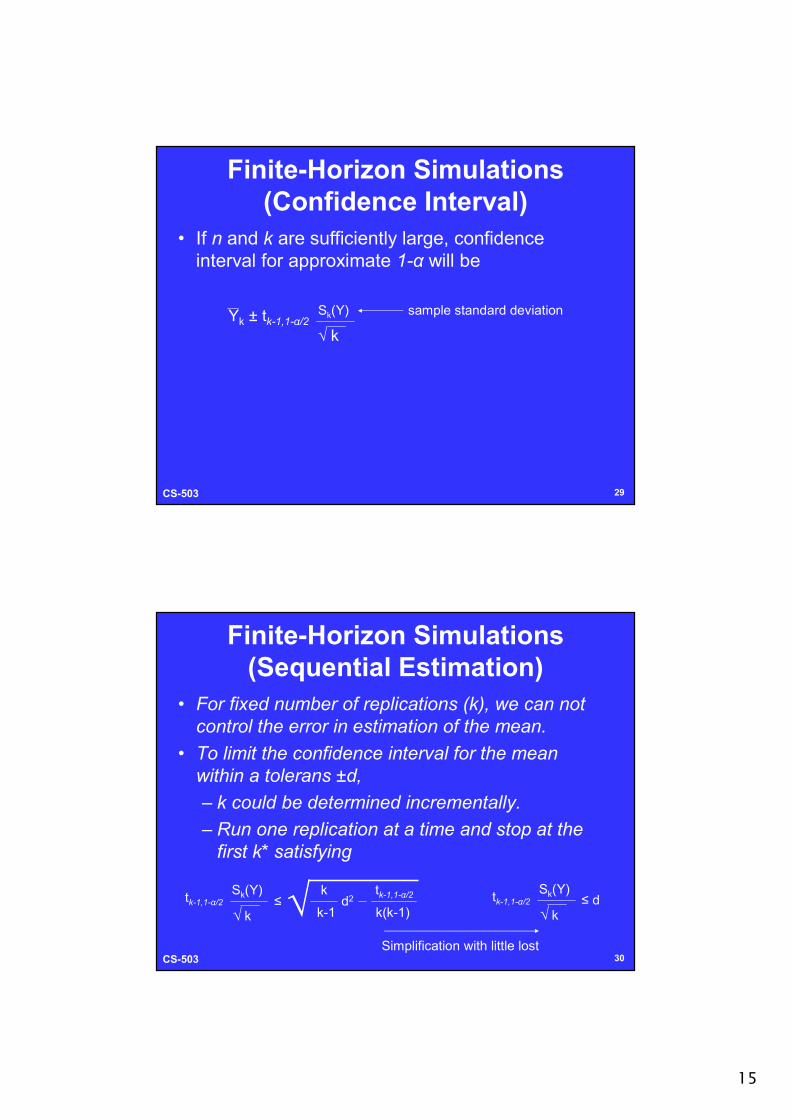
• If n and k are sufficiently large, confidence interval for approximate 1-α will be
Yk ± tk-1,1-α/2Sk(Y)
√ k
sample standard deviation
30CS-503
Finite-Horizon Simulations(Sequential Estimation)
• For fixed number of replications (k), we can not control the error in estimation of the mean.
• To limit the confidence interval for the mean within a tolerans ±d,
– k could be determined incrementally.
– Run one replication at a time and stop at the first k* satisfying
tk-1,1-α/2Sk(Y)
√ k≤
k-1 k(k-1)
k tk-1,1-α/2d2√ tk-1,1-α/2
Sk(Y)
√ k≤ d
Simplification with little lost

16
31CS-503
Analysis ofSteady-State Simulations
• We would like to analyse;
– Long-term behavior of system of interest
– By examining its steady-state parameters.
32CS-503
Steady-State Simulations(Removal of Initialization Bias)
• For analysing any steady-state parameter,
– A simulation should first need to be converged to a steady-state.
• But since we start a simulation from an initial state (e.g. empty, idle),
– Simulation will have a bias (warm-up interval),
– We will need to wait some time until it is converged to the steady-state.
• Therefore, our first problem will be to detect the point where convergence occurs.

17
33CS-503
Steady-State Simulations(Removal of Initialization Bias)
• Most commonly used method for reducing the bias of Xn is:
– To identify m (1≤m≤n-1), which is the index of point where convergence is about to occur, and
– Truncate the observations X1,...,Xm.
• Then the estimator for Xn will be
∑i = m+1
n
XiXn,m =1
n-m
34CS-503
Steady-State Simulations(Graphical Method of Welch)
• One of most popular graphical methods is proposed by Welch (1981, 1983).
• Suppose there is k replications, and nobservations for each replication.

18
35CS-503
Steady-State Simulations(Graphical Method of Welch)
• For the jth observation, the estimated mean is
• Method plots moving averages Xj(w) of 1 to n observations on a graph for a given time window w.
∑i = 1
k
XijXj =1
k
1
2w+1 ∑b = -w
w
Xj+b
Moving average of jth obs. = Xj(w) =
1
2j-1 ∑b = -j+1
j-1
Xj+b
w+1 ≤ j ≤ n-w
1 ≤ j ≤ w
36CS-503
Steady-State Simulations(Graphical Method of Welch)
• For instance, when w = 2
X1(2) = X1
X2(2) = 1/3 ( X1+X2+X3 )
X3(2) = 1/5 ( X1+X2+X3+X4+X5 )
X4(2) = 1/5 ( X2+X3+X4+X5+X6 )
...
Xn-2(2) = 1/5 ( Xn-4+Xn-3+Xn-2+Xn-1+Xn )
19
37CS-503
Steady-State Simulations(Graphical Method of Welch)
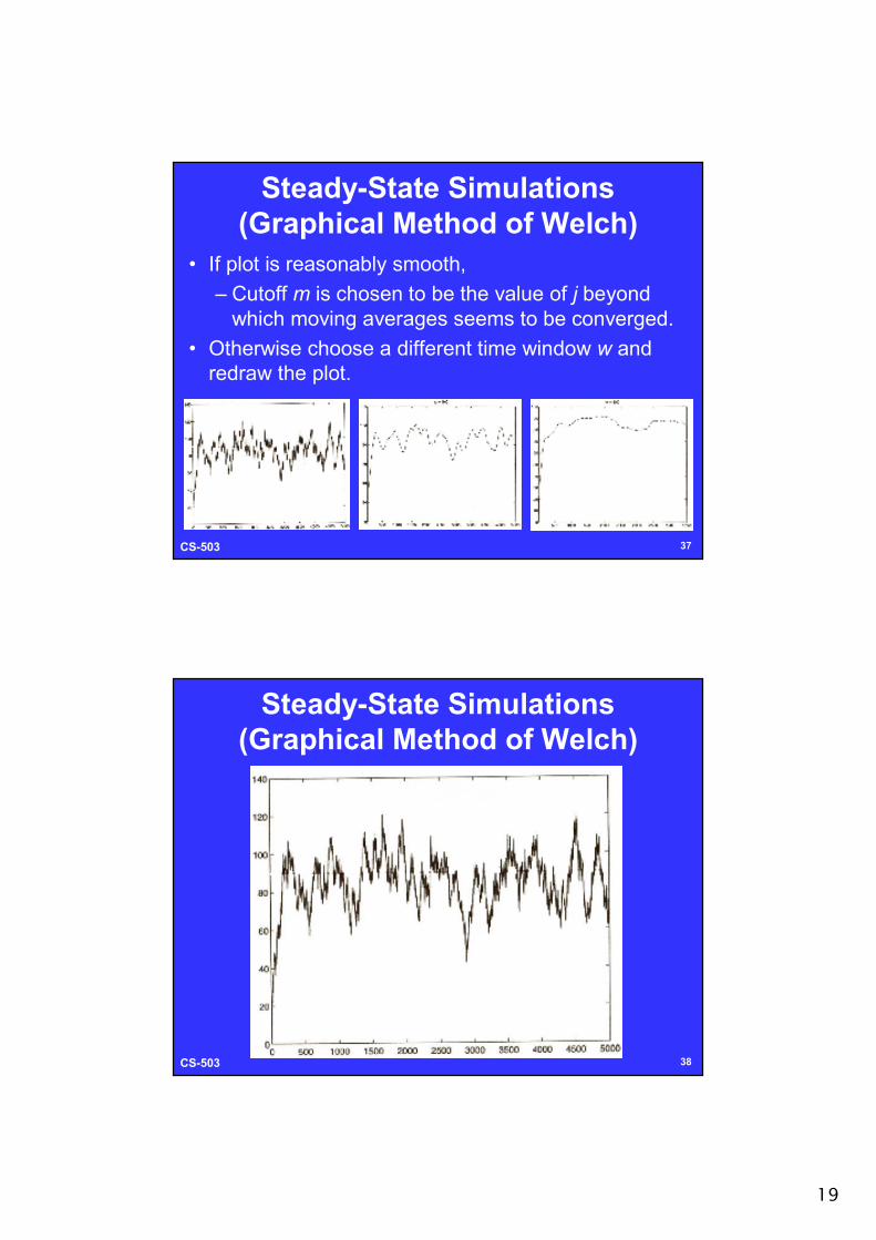
• If plot is reasonably smooth,
– Cutoff m is chosen to be the value of j beyond which moving averages seems to be converged.
• Otherwise choose a different time window w and redraw the plot.
38CS-503
Steady-State Simulations(Graphical Method of Welch)

20
39CS-503
Steady-State Simulations(Graphical Method of Welch)
40CS-503
Steady-State Simulations(Graphical Method of Welch)

21
41CS-503
Steady-State Simulations(Replication-Deletion Approach)• First determine initialization bias and cutoff m
using any method such as Welch’s.
• Run k independed replications each of length n observations, and
– If possible, make use of runs from previous bias determination phase.
• Discard m observations from each replication.
42CS-503
Steady-State Simulations(Replication-Deletion Approach)• Compute average of each replication
• Compute mean of replications
• Compute confidence interval of replications
∑j = m+1
n
XijYi =1
n-m
∑i = 1
k
YiYk =1
k
Yk ± tk-1,1-α/2Sk(Y)
√ k

22
43CS-503
Steady-State Simulations(Replication-Deletion Approach)• Important characteristics:
– As m increases for fixed n,
• Systematic error due to initial conditions decreases.
• But sampling error due to insufficient number of observations increases since variance is proportional to 1/(n-m).
n1m
44CS-503
Steady-State Simulations(Replication-Deletion Approach)• Important characteristics:
– As n increases for fixed m,
• Systematic error and sampling error decreases.
• But runs take more time to finish.
n1m

23
45CS-503
Steady-State Simulations(Replication-Deletion Approach)• Important characteristics:
– As k increases for fixed n and m,
• Systematic error does not change.
• But sampling error decreases.
n1m
k
46CS-503
Steady-State Simulations(Replication-Deletion Approach)• Drawbacks:
– Care must be taken to find a good cutoff m, and sufficiently large n and k.
– Also there is potantially wasteful of data because of truncation from each replication.
n1m
k
truncated data

24
47CS-503
Steady-State Simulations(Batch-Means Method)
• One of the approaches that tries to overcome drawbacks of replication-deletion method.
• Owes its popularity to its simplicity and effectiveness.
48CS-503
Steady-State Simulations(Classical Batch-Means Method)• Classical method:
– Divides the output of a long simulation run with n observations into k number of batches with b number of observations in each batch (b = n/k),
– Uses sample means of batches to produce point and interval estimators.
ncutoff m a long runa batch
bb b b b b b b b b
k batches
25
49CS-503
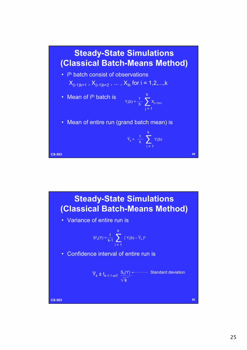
Steady-State Simulations(Classical Batch-Means Method)• ith batch consist of observations
X(i-1)b+1 , X(i-1)b+2 , ... , Xib for i = 1,2,...,k
• Mean of ith batch is
• Mean of entire run (grand batch mean) is
∑j = 1
b
X(i-1)b+jYi(b) =1
b
∑i = 1
k
Yi(b)Yk =1
k
50CS-503
Steady-State Simulations(Classical Batch-Means Method)• Variance of entire run is
• Confidence interval of entire run is
Yk ± tk-1,1-α/2Sk(Y)
√ k
∑i = 1
k
( Yi(b) – Yk )2S2
k(Y) =1
k-1
Standard deviation

26
51CS-503
Steady-State Simulations(Classical Batch-Means Method)• Drawbacks:
– Choice of batch size b is not easy.
– If b is small,
• Batch means can be highly correlated,
• Resulting confidence interval will frequently have coverage below 1-α.
– If b is large,
• There will be very few batches, and
• Potential problems with application of central limit theorem.
52CS-503
Steady-State Simulations(Classical Batch-Means Method)• Selecting batch size & number:
– Schmeiser (1982) stated that number of batches between 10 and 30 should suffice for most simulation experiments.
– Chein (1989) showed that selecting b and k proportional to √ n performs fine in some conditions (SQRT Rule).
– But in practice, SQRT rule tends to seriously underestimate variance for fixed n.

27
53CS-503
Steady-State Simulations(Overlapping Batch-Means)
• A variation of classical batch-means method.
• For a given batch size b, method uses all n-b+1overlapping batches.
• Therefore, ith batch consist of observations
Xi , Xi+1 , ... , Xi-1+b for i = 1,2,...,k
• Similar computations apply for mean and variance, but with different batch contents.
na batch
b
n-b+1 batches


