

Multi-Objective Optimisation of Water Resources Systems:
A Shared Vision
by
Walter Godoy
Thesis submitted in fulfilment of the requirement for the degree of
Doctor of Philosophy
College of Engineering and Science, Victoria University, Australia
August 2015
i
Abstract
Water resources systems are operated for many uses such as for municipal water
supply, irrigation, hydro-electric power generation, flood mitigation, storm drainage, and
for recreation. Water resources systems may also serve as places of cultural and
spiritual significance. Decision-making in this context is inherently multicriterial, often
requiring multi-disciplinary participation with a view to seeking an optimal solution or, at
best, a compromise between conflicting interests for water. Water resources planning
involves a thorough understanding of not only the quantitative aspects such as the
volumes of water harvested and released from reservoirs but also of the qualitative
factors that underpin the shared vision for the operation of water resources systems for
the benefit of all stakeholders.
The aim of this study was to develop a structured multi-objective optimisation
procedure for the optimisation of operation of water resources systems considering
climate change. For this purpose, the integration of quantitative and qualitative
information of water resources systems was achieved using a combined multi-objective
optimisation and sustainability assessment approach as part of a three-phase
procedure. This procedure was tested through the preparation of optimal operating
plans for a case study of the Wimmera-Glenelg Water Supply System (WGWSS),
assuming a range of hydro-climatic conditions. The WGWSS is located in north-
western Victoria in Australia and is a multi-purpose, multi-reservoir system which is
operated as a single water resources system; with many possible combinations of
operating rules.
Phase (1) of the procedure involved the formulation of a higher order multi-objective
optimisation problem (MOOP) for the WGWSS. A higher order MOOP is defined in this
study as a problem that is formulated with more than three objective functions. The 18
objective functions of the MOOP were developed from four major interests for water
identified in the WGWSS viz. environmental, social, consumptive, and system-wide
interests. The 24 decision variables of the MOOP represented the complex operating
rules which control the movement of water within the headworks. The constraints of
the MOOP, in terms of the physical characteristics of the WGWSS, were configured in
a simulation model. The formulation of the higher order MOOP demonstrated that the

ii
procedure provided a means to explicitly account for all the major interests for water
and to incorporate complex operating rules.
Phase (2) of the procedure involved the development of an optimisation-simulation (O-
S) model for the purposes of solving the higher order MOOP formulated in Phase (1).
The optimisation engine was used to perform the search for candidate optimal
operating plans and the simulation engine was used to emulate the behaviour of the
system under the influence of these candidate optimal operating plans. The setup of
the optimisation engine was based on a widely used evolutionary algorithm and the
setup of the simulation engine involved the replacement of an available simulation
model with a surrogate model that had greater flexibility and stability in terms of
changing from one operating plan to another. Three hydro-climatic data sets were
used to represent historic conditions and future climate conditions assuming a range of
greenhouse gas emissions. The setup of the optimisation engine was described in
terms of the genetic operators (i.e. selection, crossover, and mutation) and the
optimisation parameters (i.e. genetic operator settings, population size etc).
Phase (3) of the procedure involved the development of an analytical approach which
used the Sustainability Index ( ) to evaluate optimal operating plans. The was
used to aggregate the 18 objectives of the higher order MOOP, either separately in
terms of the major interests for water, or collectively in terms of the sustainability of the
WGWSS. The was shown to have the flexibility to include a range of interests for
water together with scaling characteristics that did not obscure poor performance. The
provided a simple means to rank optimal operating plans along the Pareto front with
respect to all 18 objectives. The Pareto front is the set of optimal trade-offs between
the conflicting objectives. Moreover, the was extended to incorporate stakeholders’
preferences for the purposes of selecting preferred Pareto-optimal operating plan(s)
under the three hydro-climatic conditions mentioned earlier in Phase (2). The resulting
Weighted Sustainability Index ( ) for the th stakeholder had all the benefits of the
in terms of flexibility and scalability as described earlier.
Importantly, the key innovation of this procedure is that it combines the formation of
Pareto fronts for a range of hydro-climatic conditions with sustainability principles to
deliver a practical tool that can be used to evaluate and select preferred Pareto-optimal
solutions of higher order MOOPs for any water resources system.

iii
Declaration
“I, Walter Rafael Godoy, declare that the PhD thesis entitled ‘Multi-Objective
Optimisation of Water Resources Systems: A Shared Vision’ is no more than 100,000
words in length including quotes and exclusive of tables, figures, appendices,
bibliography, references and footnotes. This thesis contains no material that has been
submitted previously, in whole or in part, for the award of any other academic degree or
diploma. Except where otherwise indicated, this thesis is my own work.”
Signature: Date: 20 September 2015

iv
Acknowledgements
I would like to express my gratitude to my family and friends who gave me the
possibility to complete this thesis. In particular:
My wife, Doris, and my children, Evelyn and Thomas, for their patience and
support in times of much hardship during this research and preparation of this
thesis. This work in part is dedicated to them for my absence as a loving
husband and father;
My supervisor, Prof. Chris Perera, for his guidance in my research and tireless
efforts in reviewing each chapter of this thesis. Much appreciation is extended
to Chris for his understanding of my personal struggles and in his belief that I
was a worthy candidate;
My supervisor, Dr. Andrew Barton, for the opportunity to apply for candidature
and his belief in that my practical knowledge of water resources engineering
was of valuable contribution to science. Much appreciation is extended to
Andrew for his strategic thinking in the application of this study to real-world
water resources problems;
I would also like to thank the three examiners of this thesis (Prof. D. Nagesh
Kumar, Prof. George Kuczera, and an anonymous examiner) for their well
considered comments which have greatly improved the quality of this thesis;
My mum and dad, Aida and Rodolfo, whom I know would be proud of the effort
that has gone into this piece of work. Much appreciation goes to my mum for
her assistance with my family at times when I was absent. This work, in part, is
dedicated to them for instilling in me the belief that I can always do better;
I thank the Australian Research Council, GWMWater, and Victoria University for
the financial assistance provided to this research project. I could not have
pursued my PhD research if not for the scholarship funded by these
organisations; and
My wife and sister-in-law, Claudia, for their assistance in the review and
collation of the draft thesis for submission.

v
Table of Contents
Abstract ......................................................................................................................... i
Declaration ................................................................................................................... iii
Acknowledgements ....................................................................................................... iv
CHAPTER 1. INTRODUCTION............................................................................... 1-1
1.1 Background ................................................................................................... 1-1
1.2 Aims of the study .......................................................................................... 1-4
1.3 Research methodology ................................................................................. 1-5
1.3.1 Phase (1) - Formulation of MOOP ............................................................ 1-6
1.3.1.1 Identification of major interests for water ........................................... 1-6
1.3.1.2 Specification of objective functions, decision variables, and
constraints ........................................................................................ 1-6
1.3.2 Phase (2) - Development of O-S model .................................................... 1-7
1.3.2.1 Setup of optimisation engine ............................................................. 1-7
1.3.2.2 Setup of simulation engine ................................................................ 1-8
1.3.3 Phase (3) - Selection of preferred Pareto-optimal solution(s) ................... 1-8
1.3.3.1 Design of an analytical approach to evaluate candidate optimal
operating plans ................................................................................. 1-8
1.3.3.2 Evaluation of optimal operating plans under a range of hydro-
climatic conditions ............................................................................. 1-9
1.3.4 Concluding remarks on methodology ....................................................... 1-9
1.4 Significance of the research ....................................................................... 1-10
1.5 Innovations of the research ........................................................................ 1-12
1.6 Layout of this thesis ................................................................................... 1-13
CHAPTER 2. MULTI-OBJECTIVE OPTIMISATION MODELLING IN WATER
RESOURCES PLANNING - A REVIEW ........................................... 2-1
2.1 Introduction ................................................................................................... 2-1
vi
2.2 Water resources planning ............................................................................ 2-3
2.2.1 Water resources systems ......................................................................... 2-3
2.2.2 Moving towards sustainability ................................................................... 2-6
2.2.3 Future climate considerations ................................................................... 2-8
2.2.4 Systems analysis techniques ................................................................. 2-12
2.3 Multi-objective optimisation ....................................................................... 2-14
2.3.1 Classical and non-classical methods ...................................................... 2-17
2.3.2 Optimisation-simulation modelling .......................................................... 2-18
2.3.2.1 Optimisation engine ........................................................................ 2-22
2.3.2.2 Simulation engine............................................................................ 2-25
2.3.3 Higher order multi-objective optimisation problems ................................ 2-26
2.3.4 Selection of most preferred optimal solution ........................................... 2-31
2.4 Summary ...................................................................................................... 2-34
CHAPTER 3. A SHARED VISION FOR THE WIMMERA-GLENELG WATER
SUPPLY SYSTEM ............................................................................ 3-1
3.1 Introduction ................................................................................................... 3-1
3.2 The Wimmera-Glenelg Water Supply System ............................................. 3-6
3.2.1 The study area ......................................................................................... 3-6
3.2.2 The Wimmera-Glenelg REALM model ................................................... 3-10
3.2.3 Stakeholders’ interests for water ............................................................ 3-12
3.2.3.1 Environmental ................................................................................. 3-14
3.2.3.2 Social .............................................................................................. 3-16
3.2.3.2.1 Recreation ................................................................................... 3-16
3.2.3.2.2 Cultural ........................................................................................ 3-18
3.2.3.2.3 Water quality ................................................................................ 3-19
3.2.3.3 Consumptive ................................................................................... 3-20
3.2.3.4 System-wide ................................................................................... 3-22
3.2.4 Performance metrics .............................................................................. 3-24
3.2.4.1 Reliability ........................................................................................ 3-25
3.2.4.2 Resiliency ....................................................................................... 3-27
3.2.4.3 Vulnerability .................................................................................... 3-28

vii
3.3 A higher order MOOP for the Wimmera-Glenelg Water Supply System .. 3-29
3.3.1 Objective functions ................................................................................. 3-31
3.3.1.1 Environmental ................................................................................. 3-32
3.3.1.2 Social .............................................................................................. 3-32
3.3.1.3 Consumptive ................................................................................... 3-33
3.3.1.4 System-wide ................................................................................... 3-33
3.3.2 Decision variables .................................................................................. 3-33
3.3.2.1 Priority of supply ............................................................................. 3-35
3.3.2.2 Flood reserve volume ...................................................................... 3-39
3.3.2.3 Share of environmental allocation ................................................... 3-40
3.3.2.4 Flow path ........................................................................................ 3-43
3.3.2.5 Storage maximum operating volume ............................................... 3-48
3.3.2.6 Storage target and draw down priority ............................................. 3-50
3.3.3 Constraints ............................................................................................. 3-54
3.3.3.1 Bounds on variables ........................................................................ 3-55
3.3.3.2 Integer constraints ........................................................................... 3-55
3.3.3.3 Statutory constraints ....................................................................... 3-56
3.3.3.4 Physical constraints ........................................................................ 3-56
3.4 Optimisation-simulation model setup ........................................................ 3-56
3.4.1 Simulation engine ................................................................................... 3-58
3.4.1.1 System file ...................................................................................... 3-59
3.4.1.2 Input data ........................................................................................ 3-64
3.4.1.2.1 Hydro-climatic inputs .................................................................... 3-64
3.4.1.2.2 Water demands ............................................................................ 3-66
3.4.2 Optimisation engine ............................................................................... 3-66
3.4.2.1 Genetic operators............................................................................ 3-69
3.4.2.1.1 Selection ...................................................................................... 3-70
3.4.2.1.2 Crossover .................................................................................... 3-71
3.4.2.1.3 Mutation ....................................................................................... 3-72
3.4.2.2 Optimisation parameters ................................................................. 3-73
3.4.2.2.1 Sensitivity analysis ....................................................................... 3-75
3.5 Sustainability Indices for the Wimmera-Glenelg Water Supply System .. 3-77
3.5.1 The Sustainability Index ......................................................................... 3-78
3.5.2 The Weighted Sustainability Index ......................................................... 3-83

viii
3.6 Summary ...................................................................................................... 3-87
CHAPTER 4. ANALYSIS OF OPTIMAL OPERATING PLANS USING THE
SUSTAINABILITY INDEX ( ) ......................................................... 4-1
4.1 Introduction ................................................................................................... 4-1
4.2 A lower order MOOP - one user group ........................................................ 4-7
4.2.1 Problem formulation and model setup ...................................................... 4-7
4.2.2 Modelling results and discussion .............................................................. 4-8
4.2.2.1 Objective space ................................................................................ 4-8
4.2.2.2 Decision space ................................................................................ 4-13
4.2.2.3 Discussion....................................................................................... 4-19
4.2.3 Conclusions ........................................................................................... 4-20
4.3 A series of higher order MOOPs – all user groups ................................... 4-21
4.3.1 Problem formulation and model setup .................................................... 4-22
4.3.2 Modelling results and discussion ............................................................ 4-25
4.3.2.1 Objective space .............................................................................. 4-25
4.3.2.2 Decision space ................................................................................ 4-26
4.3.2.3 Discussion....................................................................................... 4-36
4.3.3 Conclusions ........................................................................................... 4-39
4.4 A higher order MOOP for the Wimmera-Glenelg Water Supply System
– all user groups ......................................................................................... 4-41
4.4.1 Problem formulation and model setup .................................................... 4-41
4.4.2 Modelling results and discussion ............................................................ 4-42
4.4.2.1 Objective space .............................................................................. 4-42
4.4.2.2 Decision space ................................................................................ 4-46
4.4.2.3 Discussion....................................................................................... 4-55
4.4.3 Conclusions ........................................................................................... 4-57
4.5 Summary ...................................................................................................... 4-58
CHAPTER 5. SELECTION OF PREFERRED OPTIMAL OPERATING PLANS
UNDER VARIOUS FUTURE HYDRO-CLIMATIC SCENARIOS ....... 5-1
5.1 Introduction ................................................................................................... 5-1

ix
5.2 A MOOP for the Wimmera-Glenelg Water Supply System under two
plausible future GHG emissions scenarios ................................................ 5-8
5.2.1 Problem formulation and model setup ...................................................... 5-8
5.2.1.1 Run (A2) – The low to medium level GHG emission scenario ........... 5-8
5.2.1.2 Run (A3) – The medium to high level GHG emission scenario ........ 5-10
5.2.2 Modelling results and discussion ............................................................ 5-10
5.2.2.1 Objective space .............................................................................. 5-10
5.2.2.2 Decision space ................................................................................ 5-18
5.2.2.3 Discussion....................................................................................... 5-27
5.2.3 Conclusions ........................................................................................... 5-35
5.3 Selection of preferred optimal operating plan for the WGWSS ............... 5-38
5.3.1 Stakeholder preferences ........................................................................ 5-38
5.3.2 Post-processing results and discussion .................................................. 5-42
5.3.2.1 Objective space .............................................................................. 5-42
5.3.2.2 Decision space ................................................................................ 5-45
5.3.2.3 Discussion....................................................................................... 5-45
5.3.3 Conclusions ........................................................................................... 5-49
5.4 Summary ...................................................................................................... 5-50
CHAPTER 6. SUMMARY, CONCLUSIONS AND RECOMMENDATIONS ............. 6-1
6.1 Summary ........................................................................................................ 6-1
6.1.1 Formulation of MOOP .............................................................................. 6-3
6.1.2 Development of O-S model ...................................................................... 6-6
6.1.3 Selection of preferred Pareto-optimal solution(s) ...................................... 6-7
6.2 Conclusions................................................................................................... 6-9
6.2.1 Additional benefits of using the Sustainability Index ( ) in higher
order MOOPs .......................................................................................... 6-9
6.2.2 The results of the O-S modelling runs for the three hydro-climatic
conditions (i.e. the robust optimal operating plans) ................................ 6-10
6.2.3 The results of the selection process as applied to the robust optimal
operating plans (i.e. preferred optimal operating plans) ......................... 6-11
6.3 Recommendations ...................................................................................... 6-11
x
6.3.1 Increasing the fidelity of the Wimmera-Glenelg REALM model ............... 6-12
6.3.2 Investigating potential developments to the optimisation process using
the ..................................................................................................... 6-13
6.3.3 Application to real-world planning study ................................................. 6-13
7.0 REFERENCES ................................................................................. 7-1
List of Tables
Table 3.1 Headworks storages in the WGWSS (as in Wimmera-Glenelg
REALM model) ................................................................................. 3-9
Table 3.2 Shares of Water Available (source: VGG, 2010) ............................. 3-22
Table 3.3 Method for estimating Water Available in the WGWSS
(VGG, 2010) ................................................................................... 3-24
Table 3.4 Water management planning decisions for the WGWSS ................ 3-34
Table 3.5 Relationship between the volume held in Lake Bellfield versus
the proportion supplied to consumptive users (19) to (30) from
Lake Bellfield via the Bellfield-Taylors pipeline
(as per the base case operating plan) ............................................. 3-46
Table 3.6 Decision variables ( ) and corresponding full supply volume
( for six headworks storages in the WGWSS ......................... 3-49
Table 3.7 Supply systems and draw down priorities for the headworks
storages of the WGWSS (as per the base case operating plan) ..... 3-50
Table 3.8 Second, third and fourth points of the storage target curves
expressed in terms of decision variables values,
and (as per the base case operating plan) ........................... 3-54
Table 3.9 Six O-S model runs used in sensitivity analysis .............................. 3-75
Table 3.10 Mean crowding distance ( ) of the optimal operating plans for a
range of and values assuming population sizes and
.......................................................................................... 3-76
Table 4.1 Water management planning decisions for the WGWSS .................. 4-3
Table 4.2 Change in reliability, resiliency, and vulnerability of operating
Plan no. 1 to Plan no. 6 relative to the base case operating plan
(BC01) ............................................................................................ 4-11

xi
Table 4.3 Objective function value, Sustainability Index, and crowding
distance for optimal operating plans ................................................ 4-12
Table 4.4 Storage maximum operating volumes (in ML) and Sustainability
Index (italics) for the six optimal operating plans for the lower
order MOOP ................................................................................... 4-20
Table 4.5 Settings of decision variables for optimisation-simulation
modelling scenarios Run (A1) to Run (G1) ...................................... 4-25
Table 4.6 Objective function values, Component-level Index values, and
Sustainability Index values for the base case operating plan
(BC01) and for two optimal operating plans under Run (A1) i.e.
Plan no. 11 - highest ranked operating plan, and Plan no. 6 -
lowest ranked operating plan ...................................................... 4-44
Table 4.7 Priority of supply decisions for the base case operating plan
(BC01) and for two optimal operating plans under Run (A1) i.e.
Plan no. 11 - highest ranked operating plan, and Plan no. 6 -
lowest ranked operating plan ...................................................... 4-47
Table 4.8 Flood reserve volume decisions for the base case operating plan
(BC01) and for two optimal operating plans under Run (A1) i.e.
Plan no. 11 - highest ranked operating plan, and Plan no. 6 -
lowest ranked operating plan ...................................................... 4-48
Table 4.9 Share of environmental allocation decisions for the base case
operating plan (BC01) and for two optimal operating plans under
Run (A1) i.e. Plan no. 11 - highest ranked operating plan, and
Plan no. 6 - lowest ranked operating plan ................................... 4-49
Table 4.10 Flow path decisions for the base case operating plan (BC01) and
for two optimal operating plans under Run (A1) i.e. Plan no. 11 -
highest ranked operating plan, and Plan no. 6 - lowest ranked
operating plan ............................................................................. 4-51
Table 4.11 Storage maximum operating volume (MOV) decisions for the
base case operating plan (BC01) and for two optimal operating
plans under Run (A1) i.e. Plan no. 11 - highest ranked
operating plan, and Plan no. 6 - lowest ranked operating plan .... 4-52
Table 4.12 Storage draw down priority and storage target decisions for the
base case operating plan (BC01) and for two optimal operating

xii
plans under Run (A1) i.e. Plan no. 11 - highest ranked
operating plan, and Plan no. 6 - lowest ranked operating plan .... 4-53
Table 5.1 Water management planning decisions for the WGWSS .................. 5-3
Table 5.2 Key specifications for O-S modelling runs referred to in Chapter 5 ... 5-7
Table 5.3 Objective function values, Component-level Index values, and
Sustainability Index values for the base case operating plan and
Plan no. 8 under Run (A2) .............................................................. 5-12
Table 5.4 Objective function values, Component-level Index values, and
Sustainability Index values for various operating plans under
historic hydro-climatic conditions and two GHG emission
scenarios ........................................................................................ 5-17
Table 5.5 Priority of supply decisions for the base case operating plan and
for the highest ranked operating plans under Run (A1),
Run (A2), and Run (A3) .................................................................. 5-19
Table 5.6 Flood reserve volume decisions for the base case operating plan
and for the highest ranked operating plans under Run (A1),
Run (A2), and Run (A3) .................................................................. 5-20
Table 5.7 Share of environmental allocation decisions for the base case
operating plan and for the highest ranked operating plans
under Run (A1), Run (A2), and Run (A3) ........................................ 5-21
Table 5.8 Flow path decisions for the base case operating plan and for the
highest ranked operating plans under Run (A1), Run (A2), and
Run (A3) ......................................................................................... 5-23
Table 5.9 Storage maximum operating volume (MOV) decisions for the
base case operating plan and for the highest ranked operating
plans under Run (A1), Run (A2), and Run (A3) ............................... 5-24
Table 5.10 Storage draw down priority and storage target decisions for the
base case operating plan and for the highest ranked operating
plans under Run (A1), Run (A2), and Run (A3) ............................... 5-25
Table 5.11 Water balance for operating plans under historic hydro-climatic
conditions and two GHG emission scenarios – ML/year ................. 5-29
Table 5.12 Values of Component-level Index and Sustainability Index
(without and with stakeholder preferences) for the shortlisted
robust optimal operating plans under historic hydro-climatic
conditions and two GHG emission scenarios .................................. 5-44

xiii
List of Figures
Figure 2.1 Sample min-min multi-objective optimisation problem ..................... 2-15
Figure 2.2 Sample min-min multi-objective optimisation problem (with
colour-coding to show the dominance test results) .......................... 2-16
Figure 2.3 Schematic of a GA-based optimisation–simulation modelling
approach ......................................................................................... 2-19
Figure 2.4 Cartesian system (left) and corresponding parallel co-ordinate
(right) .............................................................................................. 2-27
Figure 2.5 An Interactive Decision Map (IDM) (source: Lotov et al., 2005) ....... 2-28
Figure 2.6 Three-dimensional plot using cone-shaped markers with varying
colours, orientation, and size (source: Kollat et al., 2011) ............... 2-29
Figure 3.1 The WGWSS showing Supply Systems 1 to 7 .................................. 3-7
Figure 3.2 Schematic of the Wimmera-Glenelg Water Supply System (not to
scale) ................................................................................................ 3-8
Figure 3.3 The Wimmera-Glenelg REALM model ............................................ 3-11
Figure 3.4 Value tree of the higher order MOOP for the WGWSS .................... 3-30
Figure 3.5 Lake Wartook flood target curve ..................................................... 3-40
Figure 3.6 Storage target curves for supply system (1)
(as per the base case operating plan) ............................................. 3-52
Figure 3.7 Storage target curves for supply system (2)
(as per the base case operating plan) ............................................. 3-52
Figure 3.8 Flow chart of optimisation-simulation model used to solve the
higher order MOOP for the WGWSS .............................................. 3-57
Figure 3.9 The WMPP2104.sys file .................................................................. 3-59
Figure 3.10 The Wimmera-Glenelg REALM model ............................................ 3-61
Figure 3.11 Comparison of total volume held in headworks storages ................ 3-63
Figure 3.12 Elitist Non-Dominated Sorting Genetic Algorithm (NSGA-II) ............ 3-67
Figure 3.13 The crowding distance calculation used in NSGA-II ........................ 3-68
Figure 3.14 Tournament selection operator ....................................................... 3-70
Figure 3.15 single-point crossover operator ....................................................... 3-72
Figure 3.16 random mutation operator ............................................................... 3-73
Figure 3.17 Value tree of the higher order MOOP for the WGWSS .................... 3-78
Figure 3.18 The Sustainability Index ( ) for the WGWSS ................................. 3-79

xiv
Figure 3.19 The th stakeholder’s Weighted Sustainability Index ( ) for the
WGWSS ......................................................................................... 3-86
Figure 4.1 Schematic of the Wimmera-Glenelg Water Supply System (not to
scale) ................................................................................................ 4-1
Figure 4.2 3-D (x-y-z) plot of six optimal operating plans for the lower order
MOOP and the base case operating plan (BC01) ............................. 4-9
Figure 4.3 2-D (x-y) plot of Pareto front for the lower order MOOP .................. 4-10
Figure 4.4 2-D (x-z) plot of Pareto front for the lower order MOOP .................. 4-10
Figure 4.5 2-D (y-z) plot of Pareto front for the lower order MOOP .................. 4-11
Figure 4.6 Sustainability Index curve for a lower order MOOP ......................... 4-13
Figure 4.7 Sustainability Index curve and corresponding decision variable
( ) for maximum operating volume at Rocklands Reservoir ....... 4-14
Figure 4.8 Sustainability Index curve and corresponding decision variable
( ) for maximum operating volume at Toolondo Reservoir ......... 4-15
Figure 4.9 Sustainability Index curve and corresponding decision variable
( ) for maximum operating volume at Taylors Lake ................... 4-15
Figure 4.10 Sustainability Index curve and corresponding decision variable
( ) for maximum operating volume at Lake Bellfield ................... 4-17
Figure 4.11 Sustainability Index curve and corresponding decision variable
( ) for maximum operating volume at Lake Lonsdale (via inlet) . 4-18
Figure 4.12 Sustainability Index curve and corresponding decision variable
( ) for maximum operating volume at Lake Lonsdale (via
outlet) ............................................................................................. 4-18
Figure 4.13 Sustainability Index curve and corresponding decision variable
( ) for maximum operating volume at Moora Moora Reservoir... 4-19
Figure 4.14 Sustainability Index curves for optimisation-simulation modelling
scenarios: Run (A1) to Run (G1) ..................................................... 4-26
Figure 4.15 Sustainability Index curve and corresponding decision variable
( ) for maximum operating volume at Rocklands Reservoir -
Run (A1) and Run (F1) ................................................................... 4-27
Figure 4.16 Relative frequency distribution of decision variable ( )
maximum operating volume at Rocklands Reservoir - Run (A1)
and Run (F1) .................................................................................. 4-28
xv
Figure 4.17 Sustainability Index curve and corresponding decision variable
( ) for maximum operating volume at Toolondo Reservoir -
Run (A1) and Run (F1) ................................................................... 4-29
Figure 4.18 Relative frequency distribution of decision variable ( )
maximum operating volume at Toolondo Reservoir - Run (A1)
and Run (F1) .................................................................................. 4-29
Figure 4.19 Sustainability Index curve and corresponding decision variable
( ) for maximum operating volume at Taylors Lake - Run (A1)
and Run (F1) .................................................................................. 4-30
Figure 4.20 Relative frequency distribution of decision variable ( )
maximum operating volume at Taylors Lake - Run (A1) and
Run (F1) ......................................................................................... 4-30
Figure 4.21 Sustainability Index curve and corresponding decision variable
( ) for maximum operating volume at Lake Bellfield - Run (A1)
and Run (F1) .................................................................................. 4-31
Figure 4.22 Relative frequency distribution of decision variable ( )
maximum operating volume at Lake Bellfield - Run (A1) and
Run (F1) ......................................................................................... 4-32
Figure 4.23 Sustainability Index curve and corresponding decision variable
( ) for maximum operating volume at Lake Lonsdale (inlet) -
Run (A1) and Run (F1) ................................................................... 4-33
Figure 4.24 Relative frequency distribution of decision variable ( )
maximum operating volume at Lake Lonsdale (inlet) - Run (A1)
and Run (F1) .................................................................................. 4-33
Figure 4.25 Sustainability Index curve and corresponding decision variable
( ) for maximum operating volume at Lake Lonsdale (outlet) -
Run (A1) and Run (F1) ................................................................... 4-34
Figure 4.26 Relative frequency distribution of decision variable ( )
maximum operating volume at Lake Lonsdale (outlet) - Run (A1)
and Run (F1) .................................................................................. 4-34
Figure 4.27 Sustainability Index curve and corresponding decision variable
( ) for maximum operating volume at Moora Moora Reservoir
- Run (A1) and Run (F1) ................................................................. 4-35

xvi
Figure 4.28 Relative frequency distribution of decision variable ( )
maximum operating volume at Moora Moora Reservoir –
Run (A1) and Run (F1) ................................................................... 4-35
Figure 4.29 Sustainability Index curve and corresponding total maximum
operating volume for all optimal operating plans - Run (A1) and
Run (F1) ......................................................................................... 4-37
Figure 4.30 Relative frequency distribution of total maximum operating
volumes for all optimal operating plans - Run (A1) and Run (F1) .... 4-38
Figure 4.31 Sustainability Index curve for all (x56) optimal operating plans
under Run (A1) ............................................................................... 4-42
Figure 4.32 Sustainability Index curve and corresponding Component-level
Index curves for optimisation-simulation modelling scenario,
Run (A1) ......................................................................................... 4-43
Figure 5.1 Schematic of the Wimmera-Glenelg Water Supply System (not to
scale) ................................................................................................ 5-1
Figure 5.2 Sustainability Index curves for all optimal operating plans under
Run (A1), Run (A2), and Run (A3) .................................................. 5-13
Figure 5.3 Value tree of a higher MOOP of WGWSS showing preferences of
in terms of cumulative weights (in italic font) and
corresponding ratios (in bold font) ................................................... 5-40
Figure 5.4 Value tree of a higher MOOP of WGWSS showing preferences of
in terms of cumulative weights (in italic font) and
corresponding ratios (in bold font) ................................................... 5-41
Figure 5.5 Value tree of a higher MOOP of WGWSS showing preferences of
in terms of cumulative weights (in italic font) and
corresponding ratios (in bold font) ................................................... 5-42
Figure 5.6 Effect of changes in stakeholder preferences (with respect to
consumptive and environmental interests for water) on ......... 5-47

1-1
Chapter 1. Introduction
1.1 Background
Water resources systems are operated for many uses such as for municipal water
supply, irrigation, hydro-electric power generation, flood mitigation, and storm drainage
(Linsley et al., 1992). These systems also play an important social role in providing
recreational amenity and a place of cultural and spiritual significance (GWMWater
2012a; 2012b). This means that decision-making in this context is inherently
multicriterial, often requiring multi-disciplinary participation with a view to seeking a
compromise or consensus between conflicting interests for water (Belton and Stewart,
2002). Water resources planning involves a thorough understanding of not only the
quantitative aspects such as the volumes of water harvested and released from
reservoirs but also of the qualitative factors that underpin the shared vision for the
operation of water supply systems for the benefit of all stakeholders (Loucks and
Gladwell, 1999; Deb, 2001).
The Wimmera-Glenelg Water Supply System (WGWSS) is located in north-western
Victoria in Australia, and is a multi-purpose, multi-reservoir system which harvests
water from two major river systems viz. the Wimmera River and the Glenelg River. The
system is managed through a complex regime of operating rules to meet a range of
interests for water including environmental, social, and consumptive user interests.
The 12 headworks storages have their own unique hydrologic, environmental and
socio-economic attributes and are operated as a single water resources system; with
many possible combinations of operating rules (Godoy et al., 2009). In recent times
the system has undergone significant transformation from an open-channel system to a
pressurised pipeline system, with most of the associated water savings re-allocated to
the environment. This has fundamentally changed the operating rules from a harvest-
then-release regime, to one that passes a larger proportion of the system inflow for
environmental purposes. Moreover, the recent drought period caused a 78% reduction
of the average annual inflow to the system over the period July 1997 to June 2010
compared to the average annual inflow over the period July 1891 to June 1997. This

1-2
has added a new dimension to the operation of the WGWSS requiring innovative
planning to ensure uncertainties in future climate do not diminish stakeholders’ rights to
water.
Water resources planning studies are usually supported by simulation and optimisation
models which allow examination of the potential impacts of changes to hydrological
conditions, infrastructure and operating rules without incurring the costs and risk that
would be incurred if such changes were to happen to in practice (Palmer et al., 1999).
Simulation models attempt to represent all the major characteristics of a system and
are tailored to examine “what if?” scenarios (Palmer et al., 1999). Simulation modelling
is widely used in Australia and internationally to evaluate the performance of regulated
river basins (Perera et al., 2005; Kuczera et al., 2009). Optimisation models are
characterised by a numeric search technique and are better suited to address “what
should be?” questions. Of particular relevance to this thesis, is the use of combined
optimisation–simulation (O-S) models given that optimisation methods can be directly
linked with trusted simulation models (Labadie, 2004).
Many of the interests for water that exist in water resources systems are conflicting and
non-commensurable which can be generally reduced to multi-objective optimisation
problems (MOOPs) in which all objectives are considered important. MOOPs consist
of a number of objectives subject to a number of inequality and equality constraints as
described by Srinivas and Deb (1995):
Minimise/Maximise fi(x) i = 1,2,…, I
Subject to gj(x) ≤ 0 j = 1,2,…, J
hk(x) = 0 k = 1,2,…, K (1.1)
The parameter x is a p dimensional vector having p design or decision variables. The
aim is to find a vector x that satisfies J inequality constraints, K equality constraints and
minimises/maximises I objective functions. Of particular relevance to this thesis, are
those problems where three or more objectives are optimised simultaneously; the so
called many-objective (or higher order) MOOPs. Solutions to MOOPs are
mathematically expressed in terms of superior or non-dominated solutions. This
highlights the difficulty with MOOPs in that there is usually no single optimal solution
with respect to all objectives, as improving performance for one objective means that

1-3
the quality of another objective will decrease. Instead there is a set of optimal trade-
offs between the conflicting objectives known as the Pareto-optimal solutions or the
Pareto front (Deb, 2001). Deb (2001) describes the ideal multi-objective optimisation
procedure as one that involves bringing together quantitative and qualitative
information as follows:
“ Step 1: Find multiple trade-off optimal solutions with a wide range of
values for objectives.
Step 2: Choose one of the obtained solutions using higher-level
information.” (Deb, 2001, p4)
Present day water planning processes around the world highlight a desire to move
towards sustainable water resources systems that have a common view or shared
vision for the operation of the system (Loucks and Gladwell 1999). For this to occur
the MOOP needs to be formulated in such a way that it guides the search towards
optimal solutions that strive to improve the sustainability of the water resources system.
Loucks and Gladwell (1999) argued that sustainable development can only succeed
with sustainable water resources systems supporting that development. In their review
of the many definitions of sustainable development, they propose the following
definition for the management of water resources systems:
“Sustainable water resource systems are those designed and managed to
fully contribute to the objectives of society, now and in the future, while
maintaining their ecological, environmental, and hydrological integrity.”
(Loucks and Gladwell, 1999, p30)
As water resources planning is for the future, forecasts of future conditions are
essential (Linsley et al., 1992). This is especially true in planning studies that have a
long-term planning period often 50 to 100 years into the future. Fortunately, the
availability of general circulation models (GCMs) make it possible for planning
processes to incorporate the latest advances in the projection of future climate and to
understand which operating rules are paramount in an uncertain climate future. In
terms of forecasts of future conditions, the Fourth Assessment Report of the
Intergovernmental Panel on Climate Change (IPCC) stated that:

1-4
“....the warming of the climate system is unequivocal, as is now evident from
observations of increases in global average air and ocean temperatures,
widespread melting of snow and ice and rising global average sea level.”
(IPCC, 2007, p2)
1.2 Aims of the study
The aim of this project is to develop a structured procedure for the optimisation of
operation of water resources systems considering climate change. This procedure will
take explicit account of:
competing objectives concerning all major interests for water;
complex operating rules that regulate the movement of water through the
headworks system; and
a range of hydro-climatic conditions.
This procedure will be based on the ideal multi-objective optimisation approach which
firstly strives to find Pareto-optimal solutions with a wide range of values for each
objective function, followed by the selection of preferred optimal solution(s) based on
stakeholders’ preferences. The procedure will be developed and tested using the
WGWSS case study. The remainder of this section provides further details of the three
areas of study highlighted above.
Developing a thorough understanding of the major interests for water in water
resources systems provides valuable insights into the type and extent of conflict that
may exist between the different uses for water. In the WGWSS for example, many of
the 12 headworks storages having conflicting interests in terms of passing water for
provision of environmental flows; holding sufficient water in store for consumptive
needs; and holding a minimum volume in store for provision of recreation amenity. In
this example, the extent of conflict between passing water for environmental purposes
versus holding water in store for consumptive and recreation needs would probably
have a greater level of conflict than that between holding water in store for consumptive
needs versus holding water in store for recreation needs. This process of identifying

1-5
the major interests for water forms the basis of the conflicting objectives to the
optimisation problem.
Management of the natural forces of precipitation, evaporation, and streamflow
requires the collection, drainage, and transfer of water with consideration to varying
scales both spatially and temporarily; particularly in multi-reservoir systems such as the
WGWSS. Reservoir operation is a complex and challenging task, not only because of
the presence of multiple conflicting objectives but also owing to seasonal and
stochastic variations in the demand for and supply of water. Operating rules for
reservoir management include flow rates and upper limits of harvest/release and
storage target volumes throughout the year for a range of objectives as established
through the identification of the major interests for water described above. The
availability of trusted simulation models serve as useful tools for the purposes of testing
any changes to the current operating rules without incurring the costs and risks of
implementing such changes in practice.
Moreover, the inclusion of a range of hydro-climatic conditions within the structured
procedure provides a two-fold benefit. One benefit is that it allows the search for
candidate optimal operating plans to be undertaken under the various hydro-climatic
conditions. This means that the formation of Pareto fronts can be established for a
range of hydro-climatic conditions. Another benefit of the inclusion of a range of hydro-
climatic conditions is that it also allows for comparisons of the same candidate optimal
operating plan to be made under the various hydro-climatic conditions. Both these
benefits allow for a thorough testing of the robustness of optimal operating plans as
part of the selection of preferred optimal solution(s) based on stakeholders’
preferences. Moreover, the use of high quality climate projections into the future
(together with the inclusion of the major interests for water) are consistent with the
concept of sustainable development presented in Section 1.1.
1.3 Research methodology
Following a critical review of multi-objective optimisation modelling in water resources
planning, the concept of the proposed multi-objective optimisation procedure was
developed on the ideal multi-objective optimisation procedure (Deb, 2001) which
integrates quantitative and qualitative information. Firstly, an O-S model is used to

1-6
provide the quantitative information in terms of the Pareto-optimal solutions, followed
by the selection of a preferred optimal operating plan using qualitative information in
terms of stakeholder preferences. The proposed multi-objective optimisation
procedure comprises three phases as follows:
Phase (1) Formulation of MOOP;
Phase (2) Development of O-S model; and
Phase (3) Selection of preferred Pareto-optimal solution(s).
Note that while Sections 1.3.1 to 1.3.3 describe the three phases with reference to the
WGWSS case study, the proposed procedure for optimisation of operation of complex
water resources systems can be applied to any water resources system.
1.3.1 Phase (1) - Formulation of MOOP
1.3.1.1 Identification of major interests for water
Much of the information required to identify the major interests for water in the WGWSS
had already been collected as part of various recently completed planning studies. A
desktop study of this information was undertaken as part of this thesis together with a
description of the relevant parts of the simulation model which formed part of the O-S
model (as explained later in Section 1.3.2). Four broad categories of interests for water
were identified viz. environmental, social (i.e. in terms of recreation, water quality, and
cultural heritage), consumptive, and those that affected all users system-wide. As part
of this identification process, any relevant criteria by which to evaluate candidate
optimal operating plans was also identified together with the various interests for water.
For these criteria to be incorporated in the higher order MOOP, a suitable unit of
measure was developed to evaluate candidate optimal operating plans on a
quantitative basis with respect to the interests for water identified. Moreover these
performance metrics were aimed at providing the basis for meaningful dialogue
amongst the stakeholders and the decision maker (DM) in terms of the sustainability of
the interests for water identified.
1.3.1.2 Specification of objective functions, decision variables, and constraints
As with any MOOP, its formulation required the specification of objective functions,
decision variables, and constraints. The specification of the objective functions was
1-7
developed on the key assumption that the sustainability of the WGWSS was an overall
goal. This starting point led to the concept of a problem hierarchy where by each sub-
criteria level represented the sustainability of the system from a different vantage point
or perspective. For this thesis, the second level of the problem hierarchy represented
the four broad interests for water described in Section 1.3.1. This second level was
used to provide a means to describe the sustainability of the four individual interests for
water (of which collectively described the sustainability of the WGWSS from the
perspective of all interests for water). The lowest level criteria was used to represent
the objective functions for the MOOP. These lowest level criteria represented the
underlying conflicts of the problem and were directly linked to the interests for water
described in Section 1.3.1. The decision variables for the higher order MOOP were
expressed in terms of water management planning decisions representing the key
operating rules which control and regulate the water resources within the WGWSS.
The constraints of the problem were specified both in terms of the formulation of the
MOOP and also in terms of the real-world limitations of the WGWSS.
1.3.2 Phase (2) - Development of O-S model
1.3.2.1 Setup of optimisation engine
The setup of the optimisation engine was aimed at demonstrating the novelty of the
structured multi-objective optimisation procedure rather than finding Pareto fronts per
se. To that end, the O-S model includes the widely accepted evolutionary algorithm
known as the Elitist Non-dominated Sorting Genetic Algorithm (NSGA-II) developed by
Deb et al. (2002). Further details regarding NSGA-II are provided in Section 2.2.4.
The purpose of the optimisation engine was to find the best non-dominated operating
plans for evaluation using the sustainability index described in Section 1.3.3.1. The
term generation refers to a (single) iteration of the O-S model. This setup was
described in terms of the operators of the genetic algorithm (GA) and the optimisation
parameters. The genetic operators (i.e. selection, crossover, and mutation) were used
to perturb the population of candidate optimal solutions in order to create new and
possibly better performing solutions compared to those in previous generations. The
optimisation parameters (i.e. parameter representation, probability of selection,
probability of crossover, probability of mutation, stopping criteria, and population size)
were used to control the search capabilities of the GA.

1-8
1.3.2.2 Setup of simulation engine
The setup of the simulation engine was aimed at performing as many simulation runs
as was required to find the best non-dominated operating plans and to provide the
basis for a far reaching or global search for candidate optimal solutions. For this
purpose, a surrogate model was developed to provide the flexibility and stability
required to change from one operating plan to another (as required by the optimisation
engine). The REsource ALlocation Model (REALM) software package (Perera et al.,
2005) was used to simulate the harvesting and bulk distribution of water resources
within the WGWSS. Further details regarding REALM are provided in Section 2.2.4.
The derivation of the simulation data inputs representing the hydro-climatic data and
water demand data of the WGWSS was also described. The historic hydro-climatic
data extended from January 1891 to June 2009. The latest advances in the projection
of future climate were used to represent “low to medium level” and “medium to high
level” greenhouse gas (GHG) emissions. These two plausible GHG emission
scenarios extended from January 2000 to December 2099.
1.3.3 Phase (3) - Selection of preferred Pareto-optimal solution(s)
1.3.3.1 Design of an analytical approach to evaluate candidate optimal operating
plans
An analytical procedure was developed for the purposes of evaluating Pareto-optimal
operating plans. The evaluation of Pareto-optimal operating plans in this context refers
to the ranking of plans in terms of the sustainability of WGWSS; with respect to all
objectives. For this purpose, a well-established sustainability index developed and
refined by Loucks (1997), Loucks and Gladwell (1999), and Sandoval-Solis et al.
(2011) was used to aggregate all the objectives of the higher order MOOP. One of the
key attractions to this Sustainability Index ( ) was that it could be used to summarise
the performance of alternative policies from the perspective of different water users. In
the context of this thesis, this attribute was particularly beneficial as it was used to
explicitly account for all the major interests for water in the WGWSS.
1-9
1.3.3.2 Evaluation of optimal operating plans under a range of hydro-climatic
conditions
The evaluation of optimal operating plans involved applying the analytical approach
described in Section 1.3.3 to the outputs of the O-S modelling runs. In the first
instance, this evaluation process was undertaken on the optimal operating plans found
by the O-S model assuming historic hydro-climatic conditions. This allowed a direct
comparison of the O-S modelling results with the base case operating plan and to
explain the implications of new optimal operating plans against a known reference point
to the DM. In order to incorporate a range of hydro-climatic conditions, the low to
medium level and medium to high level GHG emissions described in Section 1.3.2.2
were fed to the simulation engine. This allowed for the direct search of optimal
operating plans under two plausible future GHG emission scenarios and for a
comparison with those found under historic hydro-climatic conditions.
1.3.4 Concluding remarks on methodology
The research methodology that is described in Sections 1.3.1 to 1.3.3 was influenced
by a number of important factors which are directly related to solving higher order
MOOPs, viz; (i) the slow convergence of solutions to the Pareto front; and (ii) the high
computational costs required to progress this search, particularly in the absence of
parallel computing. Research has shown that the proportion of non-dominated
solutions to the population size becomes very large as the number of objectives
increases (Fleming et al., 2005; Deb, 2011).
With respect to a population-based optimisation search, this increase in objectives has
the effect of slowing the progression (i.e. convergence) of the population of solutions to
the Pareto front. This slow convergence is largely attributed to a procedure (referred to
in this thesis as the “dominance test”) which is applied to the solutions of the population
in order to determine their non-dominance classification with respect to other solutions
of the population. For example, in the case of two very similar candidate optimal
solutions whose values of all but one of the many objectives are equal, the solution
which has the better performing objective will dominate the other, even if that
performance is minuscule. With little thought, it is easy to accept that the creation of
new candidate optimal solutions will be based on solutions that are a very similar,
resulting in slow progression towards the Pareto front.

1-10
This slow convergence means that a greater number of O-S modelling generations are
required to progress the solutions towards the Pareto front. An increase in the number
of generations requires greater computational processing effort, which in the case of
population-based optimisation searches can be addressed through distributed or
shared memory parallel computing architectures. However, such parallel computing
capabilities were not available for this study, which meant that simulation runs for all
solutions of the population had to be completed in series (i.e. one run at a time) before
the optimisation search could be executed.
For these reasons (of slow convergence and high computational costs), the number of
generations performed by the O-S model was limited to five in number (throughout this
thesis). Importantly, this is not to be confused as a research limitation given that the
novelty of this study is that of the structured multi-objective optimisation procedure
rather than finding Pareto fronts per se.
1.4 Significance of the research
A recent review of water entitlement arrangements in the WGWSS exemplifies the
significance of the research presented in thesis from a number of perspectives. The
aims of the Bulk and Environmental Entitlements Operations Review (“the review
project”) were developed as part of a series of government planning studies in Victoria
(2000 to 2011) which were tasked with re-allocating water savings from the
transformation of the open-channel delivery system to a pressurised pipeline system
(GWMWater, 2014). The overall aim of the review project was to investigate new and
potentially better operating rules for the headworks system. The scope of the review
project was based on 11 storage management objectives which were generally
consistent with the sustainability principles described earlier (GWMWater, 2014).
These storage management objectives were developed in order to ensure that the
system was operated to protect users’ rights to water.
The review project was supported by the outputs of a simulation model which has had
over 20 years of development in numerous simulation modelling studies largely for the
purposes of providing system performance variables over long term planning periods
(Godoy Consulting, 2014). In recent times, this high quality simulation model was

1-11
endorsed by the Murray-Darling Basin Authority as part of its model accreditation
process under the Murray-Darling Basin Plan (MDBA, 2011). It is worth highlighting
that researchers generally agree that the use of trusted simulation models would have
the potential of giving stakeholders and DMs greater confidence in O-S modelling
results (Maier et al., 2014). The major stakeholders involved in the review project
included the water entitlement holders, the relevant catchment management
authorities, and the Department of Environment, Land, Water & Planning. Public
submissions were also sought on the draft report to guide the decision-making process
for the decision maker (DM), being the responsible Minister administering the Water
Act 1989 (Vic).
The outputs of the study showed that current practice in the WGWSS as demonstrated
by the modelled operating rules (collectively referred to as the “base case operating
plan”) was generally consistent with stakeholders’ storage management objectives
(GWMWater, 2014). Of the 38 recommendations that were made to improve system
operation, the social interests for water in terms of recreation amenity was one area
that received the greatest level of attention (i.e. this area deals with 10 out of 38
recommendations). GWMWater (2014) adds that the majority of the public
submissions focused on the social interests for water in terms of preserving and/or
restoring recreation amenity. So much so that the recommendation to the DM is for
there to be a range of works employed to address this area of interest including
increasing the recreation water entitlement. Another area which received a great deal
of attention based on the number of recommendations (i.e. 8 out of 38
recommendations) was the need to develop more holistic and collaborative
management plans for improving environmental watering arrangements between water
agencies.
Hence, the review project highlights the following key attributes which can be
structured for many such complex water resources systems around the world and
which are the focus of this thesis, namely a desire to:
Explore new and possibly better operating rules. It is worth noting that in the
case of the review project a base case operating plan was used to provide a
known reference point for the purposes of comparing alternative operating
plans.

1-12
Consider more than two or three broad objectives by taking explicit account of
all major interests for water, particularly social interests such as for the
provision of recreation amenity.
Adopt sustainability principles in the development of a shared vision for the
operation of systems.
Adopt trusted simulation models to assist in evaluating system performance
under alternative operating plans.
It is worth noting that unlike the review project, this thesis considers climate change a
fundamental component of all water resources planning studies.
1.5 Innovations of the research
There are two major innovations to this research, viz; (i) the structured multi-objective
optimisation procedure; and (ii) the analytical approach for evaluation of candidate
optimal operating plans. Note that whilst the term operating plan is used in this section,
both innovations are relevant to the development of any water resources management
plan that may be of interest to the DM.
The novelty in the structured multi-objective optimisation procedure is that assists the
DM to develop a shared vision for the operation of complex water resource systems by
incorporating a greater level of realism into the decision-making process. Limiting
water resources problems to two or three objectives overlooks the complexities
associated with the many conflicting interests for water, the complex rules which
control the movement of water, and the hydro-climatic processes that affect the
availability of water resources. The structured multi-objective optimisation procedure
achieves this greater level of realism through, both, a holistic approach of formulating
the problem and the use of O-S modelling. The problem formulation approach sets out
a flexible basis on which to establish an overall goal for the water resources system
and to set out the underlying individual goals of the various interests for water.
Structuring the problem in this way provides the solid foundations for the evaluation of
candidate optimal operating plans (described in the second innovation below). The O-
S modelling approach allows for the incorporation of complex operating rules and the
latest advances in future climate projections through the use of trusted simulation
model. Additionally, the optimisation model that is linked to this simulation model

1-13
provides an efficient and effective means to conduct a far reaching or global search for
candidate optimal operating plans. Moreover, the problem formulation approach
provides the vital link between the individual interests for water and the search for
candidate optimal operating plans. All these attributes (of the multi-objective
optimisation procedure) provide the necessary structure, flexibility, and transparency in
the decision making process to engage stakeholders and DMs and to provide them
with the basis of meaningful dialogue for solving real-world water resources planning
problems (i.e. higher order MOOPs).
The novelty in the analytical approach which has been developed to evaluate
candidate optimal operating plans is that it provides a visual means to communicate O-
S modelling results for higher order MOOPs, in both the objective space and decision
space. This analytical approach builds on the proven capabilities of a sustainability
index developed and refined by Loucks (1997), Loucks and Gladwell (1999), and
Sandoval-Solis et al. (2011). Importantly, this Sustainability Index ( ) is capable of
quantifying sustainability by combining various performance metrics to represent the
reliability, resiliency, and vulnerability of water resources systems over time. In terms
of the objective space, ranking and plotting the against its normalised rank provides
a visual representation of the Pareto front. The gradient of the curve represents the
diversity of the operating plans with respect to the objective space. A larger gradient
represents operating plans that are more diverse than those that produce a section of
curve with a smaller gradient. In terms of the decision space, the corresponding
decision variable values may be plotted together with the curve to inform the DM
about how different planning decisions influence a system’s sustainability.
These two major innovations combine the formation of Pareto fronts for a range of
hydro-climatic conditions with sustainability principles to deliver a practical tool that can
be used to evaluate and select preferred Pareto-optimal solutions of higher order
MOOPs for any water resources system. Such innovations have the potential to set a
new precedent in the way operating plans are developed and reviewed over time.
1.6 Layout of this thesis
This first chapter provides an insight into water resources systems with regards to the
conflicting interests for water, complex operating rules, and how they are affected by

1-14
changes in system configuration and changes in climate. It describes the significance
of the research in terms of the need for optimising the operation of water resources
systems and proposes a structured procedure for the development of a shared vision
for the operation of water resources systems. It also presents the aims of the study
and describes the tasks undertaken to achieve these aims.
The second chapter presents a critical review of the literature on multi-objective
optimisation modelling in water resources planning. It describes the many challenges
that exist in the optimisation of water resources systems such as the need to explicitly
account for conflicting interests for water and the need to develop new and possibly
better ways to operate these systems under a range of hydro-climatic conditions.
Moreover, it discusses the challenges in visualising the Pareto front and in trading off
optimal solutions in higher order MOOPs.
The third chapter describes a structured procedure which is aimed at assisting the
decision maker (DM) to develop a shared vision for the operation of water resource
systems considering climate change. It deals with identifying all the major interests for
water in a complex water resource system; the formulation of a MOOP that takes
explicit account of all the major interests for water in the system; the set up of the O-S
model used to solve for this MOOP; and the indices used to analyse and select a
preferred optimal operating plan subject to stakeholders’ preferences.
The fourth chapter presents an approach for analysing Pareto-optimal operating plans
using the proposed multi-objective optimisation procedure assuming historical hydro-
climatic conditions. It presents an analytical approach that deals with ranking
alternatives; assessing the level of influence that a set of operating rules has on a
system’s sustainability; and with showing the effect of alternative operating plans on
various interests for water.
The fifth chapter applies the analytical approach presented in the fourth chapter to
MOOPs considering two plausible future greenhouse gas (GHG) emission scenarios.
It deals with evaluating and comparing the optimal operating plans that were found
under historic hydro-climatic conditions (in the fourth chapter) against the optimal
operating plans under the two GHG emission scenarios. It also deals with selecting the
most preferred optimal operating plan(s) by incorporating stakeholders’ preferences.

1-15
The sixth chapter summarises this thesis, the main conclusions and recommendations
for future work.

2-1
Chapter 2. Multi-objective optimisation modelling in water resources planning - a review
2.1 Introduction
This chapter presents a critical review of the literature on multi-objective optimisation
modelling in water resources planning. Specifically, it deals with (i) the various aspects
of water resources planning and the multi-criterial nature of problems concerning the
planning and operation of multi-purpose, multi-reservoir water resources systems; and
(ii) multi-objective optimisation as a means by which to solve such complex problems
by finding new and possibly better ways to operate water resources systems,
particularly in an uncertain climate future. For this purpose, reference is made to the
Wimmera-Glenelg Water Supply System (WGWSS) case study which is located in
north-western Victoria (Australia). The WGWSS is a multi-purpose, multi-reservoir
system which is managed through a complex regime of operating rules to meet a range
of interests for water (Godoy et al., 2009).
Water resources systems are operated for many uses such as municipal water supply,
irrigation, hydro-electric power generation, flood mitigation, and storm drainage (Linsley
et al., 1992). These systems also play an important social role in providing recreational
amenity and as a place of cultural and spiritual significance (GWMWater, 2012a;
2012b). Optimal operation of water resources systems requires careful planning in
order to ensure that the intended benefits are realised (Labadie, 2004). In many
countries around the world, water resources planning occurs at the national level in
terms of broad goals which are translated into regional actions (Linsley et al., 1992;
Castelletti and Soncini-Sessa, 2006; NWC, 2014). Present day water planning
processes around the world highlight a desire to move towards sustainable operating
plans that explicitly incorporate all interests for water and which find an optimal solution
or, at best, a compromise solution amongst all these water needs (Loucks and
Gladwell, 1999). Importantly, it has been confirmed that carbon dioxide ( ) was the
major anthropogenic greenhouse gas (GHG) contributing to the warming of the global

2-2
climate system (IPCC, 2007). Fortunately, the availability of general circulation models
(GCMs) makes it possible for planning processes to incorporate the latest advances in
the projection of future climate. GCMs are based on the theories of atmospheric
physics. Such hydro-climatic data can be incorporated into simulation and optimisation
models to examine the potential impacts of changes to not only hydrological conditions,
but also changes to infrastructure and operating rules without incurring the costs and
risk that would be incurred if such changes were to happen to in practice (Palmer et al.,
1999). Refer to Section 2.2 for details of this part of the study.
Many of the interests for water in water resources systems are conflicting and non-
commensurable which can be generally reduced to multi-objective optimisation
problems (MOOPs). Characteristically, these problems give rise to a set of optimal
solutions referred to as Pareto-optimal solutions or the Pareto front, instead of a single
optimal solution (Deb, 2001). A general MOOP consists of a number of objectives
subject to a number of inequality and equality constraints (Srinivas and Deb, 1995).
Classical and non-classical multi-objective optimisation methods are described in this
chapter and the advantages and disadvantages of using these methods are discussed
in terms of their ability to search for candidate optimal solutions in high-dimensional
problems. In recent times there has been growing interest in using evolutionary
algorithms (i.e. non-classical multi-objective optimisation methods) given that these
optimisation methods can be directly linked with trusted simulation models (Labadie,
2004). Note that in this thesis such models are referred to as optimisation–simulation
(O-S) models. Various O-S models applications are also presented highlighting the
extent to which these reflect real-world water resources systems. Moreover, the
challenges associated with the setting up of the optimisation engine and the simulation
engine of an O-S model are described. The difficulties with solving higher order
MOOPs are also presented in terms of the available techniques used to visualise the
Pareto front, and to address the issue of slow convergence to the Pareto front. The
issue of slow convergence to the Pareto front is described and various techniques
including the use of larger population sizes are discussed. With respect to selecting a
preferred optimal solution from the Pareto front of high-dimensional problems, multi-
criteria decision analysis (MCDA) techniques are presented as a means to develop a
conceptual model which can be used to represent stakeholders’ preferences and value
judgements. Refer to Section 2.3 for details of this part of the study.

2-3
2.2 Water resources planning
2.2.1 Water resources systems
As part of the process of finding optimal or compromise solutions, there are a number
of challenges that exist in the planning of water resources systems. This section
describes the national and regional planning processes that exist around the world and
highlights two important challenges which are relevant to the aims of this study, namely
the need to (i) consider more than two or three broad objectives by taking explicit
account of all major interests for water; and (ii) to incorporate the complex set of
operating rules which control the movement of water within water resources systems.
Water is controlled and regulated to serve a diverse range of purposes (Linsley et al.,
1992). In applications such as flood mitigation and storm drainage, water is controlled
to minimise damage to property, inconvenience to public, or loss of life. In other
applications such as for municipal water supply, irrigation, and hydro-electric power
generation, water may need to be regulated through a system of headwork and
balancing storages, and distributed through a network of open channels and/or
pressurised pipeline. Additionally, water also plays an important social role in providing
recreational amenity and the cultural and spiritual development of people all around the
world. Despite this diversity in the dependency on water, the collection of natural
assets and artificial structures used to control and regulate water has been commonly
referred to as water supply systems (Linsley et al., 1992). More recently however, the
term being used by water practitioners and academics is water resources systems;
given that the planning and management of such systems has a wider range of
beneficial uses (Loucks and Gladwell, 1999; GHD, 2011; GWMWater, 2012a).
Since the 1960s there has been an increasing concern about the environment given an
uncontrolled population growth and production of waste which threatens the quality of
air, land, and water (Linsley et al., 1992). This development of civilization has
increased the importance of water resources management, not only for potable and
irrigation purposes but also for public health reasons. Modern standards in personal
hygiene require significantly more water than was used a century ago. The increase in
population has increased the acreage required for agriculture and the need for
irrigation and drainage systems. The increase in industrial development has meant
that water is often used for processing food and for hydro-electric power generation.

2-4
Such is the damage that is being caused by this development of civilization, that
increasing numbers of flora and fauna are becoming endangered and extinct around
the world.
Management of the natural forces of precipitation, evaporation, and streamflow
requires the collection, drainage, and transfer of water with consideration to varying
scales both spatially and temporarily; particularly in multi-reservoir systems. Reservoir
operation is a complex and challenging decision problem, not only because of the
presence of multiple conflicting objectives but also owing to seasonal and stochastic
variations in the demand for and supply of water. Typical objectives may include
satisfaction of demands for water supply and for in-stream environmental flows;
maximising flood mitigation, hydro-electric power generation, and recreation amenity;
and protecting cultural heritage etc (Agrell et al., 1998; Emsconsultants, 2009;
GWMWater, 2012a; VEWH, 2013).
Decision variables for reservoir operation typically include flow rates and upper limits of
harvest/release and storage levels throughout the year. The seasonal aspect of
reservoir operation is not restricted to system inputs and outputs, since the operational
decisions are often closely related to seasonal activities and events. In one example
for the Shellmouth Reservoir in Manitoba (Canada), a release decision in January to
meet the demand for hydroelectric power generation may differ from the trade-off
between power supply and recreational benefits in July, when fishing and tourism are
at their peaks (Agrell et al., 1998). In another example for the WGWSS in western
Victoria (Australia), the inter-storage transfer decision from Rocklands Reservoir to
Toolondo Reservoir is an important consideration with regards to minimising
uncontrolled spills to the Glenelg River in winter/spring and minimising supply deficits
to consumptive users and the in-stream environment all year round (GHD, 2011;
GWMWater, 2012a; VEWH, 2014).
An incentive to undertake formal planning and analysis is that the investments and
long-term consequences of water resource decisions are often large in terms of time
and money expended (Agrell et al., 1998). Operation of water resources systems
requires effective planning to ensure that the intended benefits are realised (Labadie,
2004). Mooney et al. (2012) pointed out that it is important to properly identify interests
and values in the water planning decision-making process. Planning for water
resources purposes may be defined as:
2-5
“...the orderly consideration of a project from the original statement of
purpose through the evaluation of alternatives to the final decision on a
course of action.” (Linsley et al., 1992, p777)
Planning occurs at many levels within each country with a differing of purpose and
planning effort at each level. Many countries have a national planning organisation
with broad objectives to enhance economic growth and social conditions within the
country. Whilst the national planning organisation may not deal with water matters
directly, the goals it sets in terms of production of food, energy, housing etc may
require specific targets for water management. In most countries there are several
agencies that are responsible for specific areas of water management. In order to
bridge the national planning effort and the many water agencies, some countries have
formed groups that help co-ordinate water planning so that common methodologies are
established allowing for comparisons between various project studies. The U.S. Water
Resources Council, the Venezuelan Commission for Planning of Hydraulic Resources,
the European Commission, and the Australian National Water Commission are some
examples (Linsley et al., 1992; Castelletti and Soncini-Sessa, 2006; NWC, 2014).
Moreover, the broad objectives set at the national planning level have placed a greater
focus on sustainability in recent times. For example in 1980 the U.S. national
objectives were to enhance national economic development and enhance the quality of
the environment (Linsley et al., 1992). By comparison, the Australian national
objectives were aimed at delivering nationally compatible water entitlements;
conjunctive management of surface water and groundwater resources; and risk
assessments associated with changes in future water availability (NWC, 2014). This
more recent approach, which has been adopted by many countries around the world, is
based on the concept of sustainable development which is discussed in greater detail
in Section 2.2.2.
In order to delineate the planning efforts between the various regions of a country,
regional planning groups may be set up to establish regional planning processes. As
specific actions in water management are likely to have consequences both upstream
and downstream, such groups are responsible for co-ordinating the various activities
and planning efforts within the river basin or water catchment. Examples of such
regional planning groups are the Spanish Basin Agencies (Confederaciones
2-6
Hidrograficas) and the Victorian catchment management authorities (CMAs) in
Australia (Andreu et al., 2009; VEWH, 2014). The Wimmera CMA and the Glenelg-
Hopkins CMA are responsible for co-ordinating such activities in the WGWSS. The
broad national planning goal to improve environmental conditions has been translated
into 18 watering actions which are specifically aimed at protecting platypus, freshwater
catfish, Wimmera bottlebrush and other riparian vegetation in the WGWSS (VEWH,
2014). Linsley et al. (1992) pointed out that planning of specific actions such as these
is the lowest level of planning and it is this level that determines the effectiveness of
water resources management.
Another example of a regional planning process concerning the WGWSS was the
development of the Western Region Sustainable Water Strategy (DSE, 2011) which
was aimed at:
“....providing increased certainty to water users and the environment;
promoting sustainable water use; and protecting and improving the health of
waterways, aquifers, wetlands and estuaries...” (DSE, 2011, p52)
An important action under the strategy was to undertake periodic reviews of the water
sharing and operating arrangements of the WGWSS. The first review was completed
in 2014 and the outcomes of the study showed that after three years of implementing
the bulk water entitlements; management of the system was in line with the stated
objectives (GWMWater, 2014). The review was supported by simulation modelling
over a long-term planning period assuming historic and future hydro-climatic conditions
which are discussed further in Section 2.2.3.
2.2.2 Moving towards sustainability
The development and management of water resources systems is a fundamental
component of sustainable development. Loucks and Gladwell (1999) argued that
sustainable development could only succeed with sustainable water resources systems
supporting that development. In their review of the many definitions of sustainable
development, they proposed the following definition for the management of water
resources systems:
2-7
“Sustainable water resource systems are those designed and managed to
fully contribute to the objectives of society, now and in the future, while
maintaining their ecological, environmental, and hydrological integrity.”
(Loucks and Gladwell, 1999, p30)
Whilst the concept of sustainability has become a common theme in water resources
planning over the last decade, present day planning processes are challenged by a
number of factors including (i) a top-down planning focus which does not always
provide a link between the broad national goals and the diverse range of interests for
water at a local scale; and (ii) the incorporation of interests for water that are not easily
quantifiable such as those that provide a social benefit in water resources systems.
Water resources planning processes which have a top-down focus usually have broad
national goals enshrined in international directives and statutes which planners are
obliged to follow. Two studies which have set out to propose an alternative to this top-
down approach are those undertaken by Castelletti and Soncini-Sessa (2006) and
Graymore et al. (2009).
Castelletti and Soncini-Sessa (2006) proposed a nine-step participatory and integrated
water resources planning procedure as a move forward to address the lack of
communication between scientists and policy-makers, and applied it to a real-world
planning process as part of a multi-objective decision support system (DSS). The
water resources system comprised Lake Maggiore; a natural lake located south of the
Alps between Italy and Switzerland which is operated to supply downstream irrigation,
the in-stream environmental requirements of the River Ticino, and for hydropower
generation. Additionally, the lake is also operated to mitigate flood events which have
had a disastrous effect on the lake coastline population in 1993 and 2000. The
outcomes of their application resulted in nine compromise alternatives representing
different combinations of structural actions (e.g. dredging the lake outlet), normative
actions (e.g. changes to release rules at the operator’s discretion), and regulatory
actions (e.g. release rules which must be followed by the operator). Castelletti and
Soncini-Sessa (2006) claimed that the compromise alternatives were likely to have
been considered as part of (then) negotiations under the Italian-Swiss agreement of
1943 given that there was strong support by stakeholders from both countries. It is
worth highlighting that many researchers agree that DSSs are an effective means to
overcome the hindrances of multi-objective optimisation due to the ability of such

2-8
systems to place the responsibility for the success or failure of system operation on
operators and water managers rather than overly empowering computer analysts
(Labadie, 2004).
Building on the concept of DSSs, Graymore et al. (2009) suggested that a sustainability
assessment at the regional scale provided the necessary link between top-down
national goals and bottom-up local actions in order to help preserve the “...ecosystem
goods and services ...” for future generations. The authors developed a sustainability
assessment framework for regional agencies in south west Victoria (Australia) by using
a DSS which was linked to a Geographical Information System (GIS). This tool was
used to prepare maps showing sub-catchment sustainability levels in terms of the
condition of environmental, social, and economic indicators. These maps were able to
highlight those areas most in need of assistance for achieving sustainability. Graymore
et al. (2009) further suggested that the tool would be able to show variations in sub-
catchment sustainability by way of repeating the assessment process each year. The
authors claimed that such information could be used by regional water agencies as part
of planning processes that were aimed at improving regional sustainability over time.
However whilst such studies by Castelletti and Soncini-Sessa (2006) and Graymore et
al. (2009) have demonstrated the positive steps being made on the sustainability front,
one area that continues to require attention is the social assessment of water
resources management options. Mooney et al. (2012) reported on several tools they
had used to identify interests and values of water by undertaking a social impact study
of water users in South Australia and Queensland. Similar to Castelletti and Soncini-
Sessa (2006), Mooney et al. (2012) also used a participatory approach with the aim of
understanding users’ preferences and values in water allocation deliberations. Mooney
et al. (2012) argued that undertaking such assessments early in a decision-making
process improved the potential to influence the outcomes of planning processes by
integrating the assessment of management options into community engagement.
2.2.3 Future climate considerations
An important consideration in water resources planning is the need for data; most of
which represents current conditions such as land use, population, available water etc.
Additionally as water resources planning is for the future, forecasts of future conditions
are essential (Linsley et al., 1992). This is especially true in planning studies that have

2-9
a long-term planning period often 50 to 100 years into the future. Fortunately, the
availability of GCMs makes it possible for planning processes to incorporate the latest
advances in the projection of future climate. In the context of the present study, such
advances have the potential to provide a better understanding of which operating rules
are paramount in terms of the sustainability of water resources systems.
In terms of forecasts of future conditions, the Fourth Assessment Report of the
Intergovernmental Panel on Climate Change (IPCC) stated that:
“....the warming of the climate system is unequivocal, as is now evident from
observations of increases in global average air and ocean temperatures,
widespread melting of snow and ice and rising global average sea level.”
(IPCC, 2007, p2)
The Fourth Assessment Report explained that the carbon dioxide ( ) was the most
important anthropogenic GHG and that annual emissions increased by about 80%
between 1970 and 2004. The Fourth Assessment Report compared the long term
trends against corresponding data under the IPCC’s previous report i.e. the Third
Assessment Report (IPCC, 2001). Such comparisons showed that the average
surface temperature had increased from 0.6 ºC to 0.74 ºC and that the increase was
widespread over the globe; greater at higher northern latitudes. The data also showed
that global average sea level had increased at an average rate of 1.8 mm/yr and
3.1 mm/yr since 1961 and 1993 respectively. Moreover, snow and ice covered areas
had shrunk by an average of 2.7% per decade with the largest decrease in summer.
Whilst precipitation over the period 1900 to 2005 had increased significantly in eastern
parts of North and South America, and northern parts of Europe and Asia; there had
been a decline in the Mediterranean, and southern parts of Africa and Asia. Given
these hydro-climatic changes, there was a high degree of confidence that there would
be an increase in annual runoff and water availability at high latitudes and a decrease
in some dry regions in the mid-latitudes and tropics by the mid-21st century. Moreover
the projections indicated that such hydro-climatic changes would intensify water
security problems in southern and eastern Australia by 2030 (IPCC, 2007).
The Australian Academy of Science (AAS) examines the climate change science with a
focus on the impacts to Australia. According to AAS (2010), the average surface
temperature has increased by about 0.7 ºC since 1960 causing a nation-wide average
2-10
increase in the frequency of extremely hot days and a decrease in the frequency of
cold days. The long term trends in rainfall showed a significant increase over north-
western Australia, and deceases over south-western and south-eastern Australia since
1960. Importantly, these climatic changes over south-east Australia provided
conditions that were conducive to fire which among other impacts may cause water
quality problems in water resources systems. Projections showed that temperatures in
Australia were likely to be 0.5 ºC or higher by 2030 as compared to 1990 levels and
that the frequency of hot days and nights would increase (AAS, 2010).
In terms of the latest advances in the projection of climate into the future, GCMs are
widely considered to be the most advanced tools available (Anandhi et al., 2008).
These global climate projections are based on assumed future GHG emission
scenarios (IPCC, 2000). However, the coarse spatial resolution of GCMs does not
allow for predictions at the catchment or local scale and so they are incapable of
producing outputs at the fine spatial resolution needed for most hydrological studies.
To address this issue, downscaling methods have been developed which link coarse
resolution GCM outputs to surface climatic variables at finer resolutions. Downscaling
techniques can be broadly classified as either dynamic or statistical. Both techniques
have their advantages and disadvantages but one important factor to consider is that
dynamic downscaling has higher computational costs owing to its high complexity
compared to statistical downscaling methods (Sachindra et al., 2012).
Sachindra (2014) developed various models for the purposes of statistically
downscaling coarse atmospheric data to produce rainfall, evaporation, and streamflow
data sets at the catchment level. The atmospheric data was sourced from the outputs
of the National Centers for Environmental Prediction/National Center for Atmospheric
Research (NCEP/NCAR) and the Hadley Centre Coupled Model version 3 General
Circulation Model (HadCM3) given that these produced the best calibration and
validation results (Sachindra et al., 2014a). Moreover, these GCM outputs were
corrected for any bias using the tested procedure developed by Sachindra et al.
(2014b). To derive projections of global climate into the future, these GCMs are fed
data inputs that correspond to a range of concentrations of atmospheric GHGs
according to storylines that describe different levels of development in terms of
demographic, socio-economic and technological change into the future (IPCC, 2000).
Anandhi et al. (2008) suggested that a proper assessment of probable future climate
and its variability ought to be made based on various climate scenarios and so it is

2-11
preferable to consider a range of scenarios in climate impact studies in order to better
reflect the uncertainties of possible future climate.
Despite such advances in the projection of hydro-climatic conditions into the future,
water resources planning processes for the WGWSS have not incorporated these
climate projections. As explained in Section 2.2.1, the opportunity for the inclusion of
these latest advances was available as part of the development of both the Western
Region Sustainable Water Strategy (DSE, 2011) and the subsequent review of the
water sharing and operating arrangements for the WGWSS (GWMWater, 2014). Both
these planning studies were supported by simulation modelling over a long-term
planning period assuming historic hydro-climatic conditions and two future hydro-
climatic conditions. In so far as the future hydro-climatic data sets are concerned,
these were referred to as the “continuation of low flow” and the “2030 climate change”
conditions.
The continuation of low flow conditions assumed that the flows for all streams in the
WGWSS over the period January 1891 to June 1997 were factored down by the ratio
of the average streamflow over the period July 1997 to June 2009 to the average
streamflow over the period January 1891 to June 2009. This worked out to a 75%
reduction in the total average annual inflow for the WGWSS compared to the historic
hydro-climatic conditions. Jones and Durack (2005) developed the 2030 climate
change conditions using mean global warming estimates for the year 2030 provided by
GCMs. Note that unlike Sachindra (2014), Jones and Durack (2005) did not downscale
the coarse atmospheric data to the catchment level. Instead Jones and Durack (2005)
used a method that assessed the hydrological sensitivity of catchments to climate
change using mean global warming estimates for the year 2030 (as provided by
GCMs). Jones and Durack (2005) argued that their methodology provided an estimate
of the range of change in mean annual runoff which was indicative of “.... the direction
and magnitude of possible changes to water supply.” Godoy and Barton (2011)
estimated that the 2030 climate change conditions represented a 17% reduction in the
total average annual inflow for the WGWSS compared to the historic hydro-climatic
conditions.

2-12
2.2.4 Systems analysis techniques
Water resources planning studies are usually supported by simulation and optimisation
models which allow the examination of the potential impacts of changes to hydrological
conditions, infrastructure and operating rules without incurring the costs and risks that
would be incurred if such changes were to happen to in practice (Palmer et al., 1999).
Simulation models attempt to represent all the major characteristics of a system and
are tailored to examine “what if?” scenarios (Palmer et al., 1999). Simulation modelling
is widely used internationally to evaluate the performance of regulated river basins
(Perera et al., 2005; Kuczera et al., 2009). On the other hand, optimisation models are
characterised by a numeric search technique and are better suited to address “what
should be?” questions. Of particular relevance to this thesis, is the use of combined
optimisation–simulation models given that optimisation methods can be directly linked
with trusted simulation models (Labadie, 2004).
Labadie (2004) refers to simulation models as descriptive models which help answer
“what if?” questions regarding the performance of alternative operational strategies.
System operators are generally accepting of simulation models and understand their
outputs because the interpretation of results is intuitive (Labadie, 2004). Examples of
these include MODSIM (Labadie et al., 1986), WASP (Kuczera and Diment, 1988),
WATHNET (Kuczera, 1992), SWAT (Arnold et al., 1999), and REALM (Perera et al.,
2005). In Victoria (Australia) there has been heavy reliance on REALM to support
water allocation decisions by way of quantifying the impacts of proposed operational
policies on water users’ allocations (Kularathna et al., 2011; Godoy Consulting, 2014;
GWMWater, 2014). REALM is a structured computer software package that models
the harvesting and bulk distribution of water resources, usually at monthly time-steps,
within a water resources system (Perera et al., 2005). It has been developed in close
consultation with water managers and practitioners with many improvements made in
response to feedback from these users. As it has also undergone extensive testing
and has been used in many practical applications, it is considered to be the modelling
standard in Victoria. The states of Western Australia and South Australia are also
major users of REALM.
Perera et al. (2005) described the REALM setup including the preparation of input files
and the system file representing the water supply network, and the modelling output
and utility programs available for post-processing. With the aid of a graphical user

2-13
interface, the water supply network is developed using nodes representing stream
junction points, reservoirs, and water demands which are connected with carriers which
represent waterways, channels and pipes as required. At each simulation time-step,
REALM converts the network of nodes and carriers into a generic network which is
able to be solved by a network linear programming algorithm called RELAX (Bertsekas,
1991). Like other network linear programming software, RELAX uses an objective
function that minimises the sum of flow multiplied by penalty in the network to obtain
optimised carrier flows while not exceeding carrier capacity constraints and maintaining
flow balance at the nodes.
Siriwardene and Perera (2006) characterise optimisation methods as being either
deterministic or stochastic. Linear programming and dynamic programming can be
used in either of these two approaches. Deterministic methods are able to efficiently
solve large-scale optimisation problems but their main disadvantage, in so far as is
described in this thesis, is that these are unable to handle many-objective (or higher
order) problems where three or more objectives are optimised simultaneously.
Stochastic methods are designed to work directly on probabilistic descriptions of
random rather than deterministic hydrologic sequences. Whilst stochastic methods
cannot guarantee termination to optimal solutions they are often capable of undertaking
a more far reaching or global search for optimal solutions where deterministic methods
would either fail to converge or get stuck in local optima (Labadie, 2004). In terms of
the stochastic approach, heuristic programming models are based on rules-of-thumb,
experience or various analogies applied to quantitative and qualitative information
(Labadie, 2004).
One of the fastest growing areas within the heuristic programming field is the use of
multi-objective evolutionary algorithms. The reason for this is that these are robust and
can solve highly non-linear, non-convex problems. Additionally since evolutionary
algorithms are population-based searches means that these are amendable to be
implemented on distributed or shared memory parallel computing architectures which
has become an important way of reducing application run times, increasing the size
and difficulty of applications (Goldberg, 1989). Arguably, the most popular of the
evolutionary algorithm family is the genetic algorithm (GA) which uses a process
analogous to the biological processes of natural selection i.e. reproduction, crossover,
and mutation (Nicklow et al., 2010). Examples of these include the Pareto-Archived
Evolution Strategy (PAES) developed by Knowles and Corne (1999); the Strength-

2-14
Pareto Evolutionary Algorithm (SPEA2) developed by Zitzler et al. (2001); and the
more widely used Elitist Non-dominated Sorting Genetic Algorithm (NSGA-II)
developed by Deb et al. (2002). Despite these theoretical advances, the lack of
popularity in optimisation models has been largely due to the fact that these models are
more complex to develop and have greater computational requirements than simulation
models. As a consequence, problems that have used optimisation modelling have
tended to be simplified in comparison to those developed for simulation models
(Labadie, 2004).
The attraction to using prescriptive optimisation models is that optimisation methods
can be directly linked with trusted simulation models without requiring simplifications in
problem specification (Labadie, 2004). Note that in this thesis such models are
referred to as optimisation–simulation (O-S) models. These O-S models have the
ability to undertake an efficient and effective search for candidate optimal solutions in
complex water resources problems (i.e. higher order problems) and to simulate the
behaviour of complex water resources systems (i.e. multi-purpose and multi-reservoir
systems) under the influence of such candidate optimal solutions. With respect to the
many challenges facing water resources planning presented in Section 2.2, O-S
models would appear to, at least in theory, be able to handle a range of complex issues
in real-world water resources problems. Section 2.3.2 further describes the use of O-S
models in the context of MOOPs.
2.3 Multi-objective optimisation
Water resources systems are managed and operated for the benefit of a range of
interests including consumptive users, for recreation and cultural purposes, and the
environment. Many of these interests for water are conflicting and non-commensurable
which can be formulated as MOOPs. Characteristically, MOOPs give rise to a set of
optimal solutions, instead of a single optimal solution as in single-objective
optimisation. Note that single-objective optimisation involves only one objective
function (Deb, 2001). It is important to highlight that the focus of this thesis is on
MOOPs as distinct from single-objective optimisation problems. A general MOOP
consists of a number of objectives subject to a number of inequality and equality
constraints. Mathematically, the problem may be written as follows (Srinivas and Deb,
1995):

2-15
Minimise/Maximise fi(x) i = 1,2,…, I
Subject to gj(x) ≤ 0 j = 1,2,…, J
hk(x) = 0 k = 1,2,…, K (2.1)
The parameter x is a p dimensional vector having p design or decision variables. The
aim is to find a vector x that satisfies J inequality constraints, K equality constraints and
minimises/maximises the I objective functions (Srinivas and Deb, 1995). Solutions to
MOOPs are mathematically expressed in terms of superior or non-dominated points.
This highlights the difficulty with MOOPs in that there is usually no single optimal
solution with respect to all objectives, as improving performance for one objective
means that the quality of another objective will decrease. Instead there is a set of
optimal trade-offs between the conflicting objectives known as the Pareto-optimal
solutions or the Pareto front (Deb, 2001). In the case of a sample MOOP that seeks to
(i) minimise the supply deficit or shortfall in supply to an environmental water demand
(EWD); and (ii) to minimise the amount of water released to the EWD from an
upstream storage, conflict among these two objectives would generally arise in a
situation when there is a high degree of competition for water i.e. during a water
shortage. Figure 2.1 is a graphical representation of this sample two-objective
minimisation-minimisation (min-min) MOOP.
Figure 2.1 Sample min-min multi-objective optimisation problem
(A)
Volume of supply deficit to EWD
Vo
lum
e re
lea
sed
fro
m s
tora
ge t
o s
up
ply
EW
D
(C)
(D)
Candidate optimal solution
Min-Min Multi-Objective Optimisation Problem
(B)

2-16
The figure shows that the x-axis refers to the volume of supply deficit of the EWD and
the y-axis refers to the volume released from the storage to supply the EWD. Each of
the four candidate optimal solutions, Solution (A) to Solution (D), shown in Figure 2.1
have two objective values associated with it. Note that these solutions are for
illustration purposes.
Identifying the non-dominated set of solutions from a given set of solutions is similar in
principle to finding the minimum of a set of real numbers. In the latter case, two
numbers are compared to identify the smaller number using the ‘<’ relation operation.
In the former case, a solution (x1) is said to dominate the other solution (x2), if both of
the following conditions of the dominance test are true:
i. Solution (x1) is no worse than solution (x2) in all objective functions; and
ii. Solution (x1) is better than solution (x2) in at least one objective function. (2.2)
If any of the above conditions are violated, solution (x1) does not dominate solution (x2).
There are three outcomes of this dominance test, namely solution (x1) dominates
solution (x2); solution (x1) is dominated by solution (x2); or solution (x1) and solution (x2)
do not dominate each other and are said to belong to the Pareto front. Figure 2.2
shows the same solutions shown in Figure 2.1 except that the results of the dominance
test are shown by way of colour-coding, being blue shade for the set of non-dominated
Figure 2.2 Sample min-min multi-objective optimisation problem (with colour-coding
to show the dominance test results)
(A)
Volume of supply deficit to EWD
Vo
lum
e re
lea
sed
fro
m s
tora
ge t
o s
up
ply
EW
D
(B)
(C)
(D)
Non-dominated solution
Pareto front
Dominated solution
Min-Min Multi-Objective Optimisation Problem

2-17
solutions (i.e. Pareto-optimal solutions); and green shade for the dominated solutions.
For the purposes of demonstrating the application of the dominance test in
Equation 2.2, the classifications of Solution (A) to Solution (D) are determined as
follows:
Comparing Solution (A) to Solution (B) shows that Solution (A) does not
dominate Solution (B) because it violates condition (i) of Equation 2.2 in that
Solution (A) is worse than Solution (B) with respect to the volume released from
storage to supply the EWD. In fact, Solution (A) does not dominate any of the
three other solutions for the same reason. At this stage the classification of
Solution (A) cannot be confirmed without further testing as given below.
Comparing Solution (B) to Solution (A) shows that Solution (B) does not
dominate Solution (A) because it violates condition (i) of Equation 2.2 in that
Solution (B) is worse than Solution (A) with respect to the volume of supply
deficit of the EWD. Comparing Solution (B) to Solution (C) reveals that Solution
(B) does not dominate Solution (C) because it also violates condition (i) of
Equation 2.2 i.e. Solution (B) is worse than Solution (C) with respect to the
volume released from storage to supply the EWD. However, in comparing
Solution (B) to Solution (D), both conditions (i) and (ii) of Equation 2.2 are
satisfied and Solution (B) is said to dominate Solution (D). Thus, the
classification of Solution (D) as a dominated solution is confirmed by Solution
(B) which means that Solution (D) does not belong on the Pareto front.
Continuing the comparisons for Solution (C) and Solution (D) in the same way
confirm the results shown in Figure 2.2.
2.3.1 Classical and non-classical methods
Classical multi-objective optimisation methods combine multiple objectives into one
overall single objective function, . Perhaps the simplest of these is the method of
objective weighting, which may be written as follows (Srinivas and Deb, 1995):
inimise , , ote the sum of all weights 1 (2.3)
In this method the optimal solution is controlled by the weight vector . As higher level
qualitative information is required in order to set a preference for one objective over

2-18
another, classical methods tend to be highly subjective to the particular user (Deb,
2001). Notwithstanding this potential deficiency, Godoy and Barton (2011)
demonstrated that such an approach could be used to find trade-off solutions for the
environment’s regulated and unregulated entitlement considering a range of hydro-
climatic conditions using a simulation modelling.
Non-classical techniques can consider all objectives concurrently in a single run and
are not affected by the dimensionality aspect of MOOPs. Dimensionality in this context
refers to the number of objectives that are considered simultaneously as part of solving
the MOOP. Perhaps the most important characteristic of these methods is that unlike
classical methods, these tend to have the ability to undertake a more far reaching or
global search for optimal solutions. Non-classical methods are particularly useful for
water resource management problems because they tend to find the entire set of
Pareto-optimal solutions which may be used to inform a diverse and often conflicting
group of stakeholders whose decisions depend on a number of different factors. Deb
(2001) described the ideal multi-objective optimisation procedure as one that involves
bringing together quantitative and qualitative information as follows:
“ Step 1: Find multiple trade-off optimal solutions with a wide range of
values for objectives.
Step 2: Choose one of the obtained solutions using higher-level
information.” (Deb, 2001, p4)
2.3.2 Optimisation-simulation modelling
As explained in Section 2.2.4, researchers generally agree with the use of prescriptive
optimisation models given that optimisation methods can be directly linked with trusted
simulation models without requiring simplifications in problem specification (Labadie,
2004). Note that in this thesis such models are referred to as optimisation–simulation
(O-S) models. Labadie (2004) pointed out that another key reason for the growing
interest in O-S models was that the optimisation engine could include a heuristic
programming model (e.g. a genetic algorithm (GA)) which has the ability to undertake a
global search for optimal solutions and to solve highly non-linear, non-convex
problems.

2-19
Figure 2.3 illustrates the structure of an O-S model which comprises a GA-based
optimisation engine and a simulation engine. As GAs use a population-based
optimisation search technique, the O-S modelling process would commence with a
random population of solutions (shown as a green shaded circle). The process is
iterative; simulation outputs are used to evaluate the performance of the water
resources system under the influence of a given candidate optimal solution (i.e.
solution’s fitness value) which are in turn passed to the optimisation engine to find
better performing solutions than in previous iterations or generations. The O-S model
continues to iterate towards a population of Pareto-optimal solutions (shown as a red
shaded circle in Figure 2.3) until convergence has been achieved or the stopping
criterion has been reached. Many researchers describe this iterative process as one of
searching or finding candidate optimal solutions. The genetic operators (i.e. selection,
crossover, and mutation) of the GA are used to perturb the population of candidate
optimal solutions in order to create new and possibly better performing solutions
compared to those in previous generations.
Figure 2.3 Schematic of a GA-based optimisation–simulation modelling approach
The remainder of this section reviews some noteworthy proof-of-concept applications
of O-S models which have successfully used a GA-based optimisation engine.
Specifically, these applications demonstrate (i) the fidelity or degree of realism that can
(Optimisation)
No
Yes
Stopping
criterion met?
Initial
population of solutions
Search for
candidate optimal solutions:
1. Selection
2. Crossover
3. Mutation
Pareto-
optimal solutions
t = 0
Generation (t) = t+1
(Simulation)
Evaluate
candidate optimal solutions:
• System performance

2-20
be achieved by such O-S models; (ii) the number of objectives and decision variables
that have been used to achieve that fidelity; and (iii) the key study outcomes in each
case. Moreover, Sections 2.3.2.1 and 2.3.2.2 highlight the key challenges in regards to
the setting up of the optimisation engine and simulation engine.
Bekele and Nicklow (2005) described the use of an O-S model which comprised the
U.S. Department of Agriculture’s Soil and Water Assessment Tool (SWAT) and the
Strength-Pareto Evolutionary Algorithm (SPEA2). This O-S model was applied to a
four-objective MOOP, viz.; to (i) minimise the average annual sediment yield; (ii)
minimise the annual Phosphorous yield; (iii) minimise the average annual Nitrogen
yield; and (iv) maximise the average annual gross margin. The study area was Big
Creek, which is a 133 km2 agriculturally dominated catchment within the Cache River
basin located near the confluence of the Mississippi and Ohio rivers (U.S.). The
ecological significance of the Cache River basin is largely attributed to the wetland
areas which are of international significance (i.e. RAMSAR Wetland). Bekele and
Nicklow (2005) adopted three decision variables to represent the cropping decisions
associated with land use and tillage practice combinations for each of the 55 sub-
catchments of the study area. This equated to a total of 165 decisions which were
used to describe an optimal agricultural landscape. The O-S model was executed both
at the sub-catchment and catchment level to search for the best trade-off solutions.
The study demonstrated the effectiveness of using an O-S modelling approach to
quantify the extent to which certain agricultural practices influenced Nitrogen,
Phosphorus, and sediment pollution.
Mortazavi et al. (2009) tested the performance of the ε–dominance GA and the ant
colony optimisation algorithm using the Canberra Water Supply System (Australia) as
the case study. In both cases the algorithms were set up to work with a WATHNET
simulation model of the Canberra Water Supply System. WATHNET was developed
by Kuczera (1992). Mortazavi et al. (2009) presented a two-objective MOOP, viz.; to (i)
minimise present worth cost; and (ii) minimise time spent in restrictions together with
13 decision variables that were used to represent various system configurations and
operating rules. The monthly time-step simulation model was run over a period of
historic hydro-climatic conditions from 1871 to 2009. Mortazavi et al. (2009) concluded
that the GA consistently produced better results and converged faster than the ant
colony optimisation algorithm.

2-21
Building on their earlier work above, Mortazavi et al. (2012) used the ε–dominance GA
and the WATHNET software package to solve several MOOPs relating to the Sydney
Water Supply System (Australia). In all cases, the MOOPs were formulated with three
objective functions, viz.; to (i) minimise the frequency of restrictions; (ii) minimise the
present worth cost of operation and building of new infrastructure; and (iii) to minimise
environmental stress on one of many waterways. This time, 11 decision variables were
used to represent various system configurations and operating rules. Each MOOP was
formulated with the specific aim of addressing three significant shortcomings in the
literature. The first related to the maximisation of reliability of supply conflicts with the
objectives of minimising cost and environment impacts. In response to this, Mortazavi
et al. (2012) used multi-objective optimisation in order to identify trade-offs between
these conflicting objectives. The second related to the need to accurately estimate the
reliability of supply in supply systems that have a highly reliable supply, particularly
during extreme drought in which the probability of triggering drought contingency plans
is very small. For this purpose, Mortazavi et al. (2012) generated stochastic hydro-
climate data of 500 years and 10,000 years in length for use in their O-S model. The
third shortcoming related to the need to search for the best operating rules by
considering both short- and long-term operational policies.
Kularathna et al. (2011) used an O-S model which comprised the Elitist Non-dominated
Sorting Genetic Algorithm (NSGA-II) for the optimisation engine and the REALM
software package as the simulation engine. This O-S model was used to develop long-
term operating plans for the Melbourne Water Supply System (Australia) by solving a
three-objective MOOP, viz.; to (i) minimise operating and upgrade costs; (ii) maximise
environmental flows; and (iii) to maximise reliability of supply over a 30-year planning
period, assuming a monthly simulation time-step. Kularathna et al. (2011) concluded
that one of the main advantages of the O-S modelling approach was that it could be
directly linked to well-trusted simulation models and that it could be applied to long-
term planning periods. The authors also highlighted that one of the key challenges of
the O-S modelling approach was in the appropriate formulation of the optimisation
problem so that it incorporated key operating rules whilst ensuring problem complexity
was maintained at practical levels.
Similar to Kularathna et al. (2011), Godoy et al. (2012) also used an O-S model which
comprised the NSGA-II for the optimisation engine and REALM as the simulation

2-22
engine. This O-S model was used to develop long-term operating plans for the
WGWSS by solving a two-objective MOOP, viz.; to (i) maximise the reliability of supply
to consumptive users; and (ii) maximise the reliability of environmental flows over a
118-year planning period assuming historic hydro-climatic conditions at a monthly
simulation time-step. The operating plan consisted of 29 planning decisions which
captured the key operating rules for the system. The O-S modelling results were
compared to a base case (simulation-only) operating plan which represented the
existing operating plan for the system. The authors demonstrated that there were two
Pareto-optimal operating plans found by the O-S model that dominated the base case
operating plan.
2.3.2.1 Optimisation engine
Notwithstanding the importance of reviewing multi-objective evolutionary algorithms,
the focus of this thesis is the structured multi-objective optimisation procedure and the
analytical approach for evaluation of candidate optimal operating plans as described in
Section 1.5. To that end, the algorithm adopted for this thesis is not particularly
important, other than it being an accepted algorithm that is used by researchers, as is
the adopted NSGA-II. Therefore the reader is referred to the works of Zitzler and
Thiele (1999), Van Veldhuizen and Lamont (2000), and Deb et al. (2002) for
comprehensive reviews of evolutionary algorithms used in multi-objective optimisation.
The importance of the genetic operators and the optimisation parameters in GAs are
well established amongst researchers (Zitzler et al., 2000; Deb, 2001; Siriwardene and
Perera, 2006; Nicklow et al., 2010). The genetic operators (i.e. selection, crossover,
and mutation) are used to perturb the population of candidate optimal solutions in order
to create new and possibly better performing solutions compared to those in previous
generations. Once the genetic operators have been set up another important
challenge lies in specifying the parameters that control the search capabilities of the
GA i.e. parameter representation, probability of selection, probability of crossover,
probability of mutation, stopping criteria, and population size. For any given MOOP,
there is a certain element of design that is required by the analyst in order to fine-tune
the modelling outcomes. Nicklow et al. (2010) highlighted the importance of using a
carefully designed computational experiment with a clear rationale for the
representation, operators, and parameters being used as well as a clear framework for
assessing search performance.

2-23
Arguably the most common parameter representation used in GAs is in the form of an
encoding scheme that transforms the values of decision variables to a structure that
permits the genetic operations of selection, crossover, and mutation. Many of these
encoding schemes use binary strings (or chromosomes) made up of binary 0 and 1 bits
(or genes). However, Oliveira and Loucks (1997) preferred to use real-valued strings
because “......they provided a more straightforward way of representing the solutions
and permitted the design and use of efficient genetic operators that guaranteed the
feasibility of the generated solutions.” oreover to ensure the feasibility of the
operating rules, Oliveira and Loucks (1997) designed the GA so that the operators
dealt with groups of decision variables which represented one operating rule, rather
than with each variable separately. Labadie (2004) highlighted that this issue of
parameter representation was one of the continuing challenges in O-S modelling
approaches.
The primary aim of the selection operator is to make duplicates of good solutions and
eliminate bad solutions from a population, while keeping the population size constant.
The number of solutions from the population that participate in this selection process is
subject to a user-specified probability (i.e. probability of selection). In a review of GA
applications in water resources planning and management, Nicklow et al. (2010) stated
that the most familiar selection operators available in GA codes were tournament
selection, truncation selection, roulette wheel selection, and Boltzmann selection. In
their review the authors noted that the most modern codes employed a form of
tournament and/or truncation selection because these approaches were scaling
invariant (i.e. independent from the value range of the objective functions) and elitist
(i.e. the best solutions were guaranteed to survive into the next generation). Reed et
al. (2000) pointed out that scaling invariance and elitism were important properties that
had been shown to improve the effectiveness of GAs in water resources applications.
The creation of new solutions in the population is performed by the crossover and
mutation operators. Additionally, the mutation operator is required in the genetic
process in order to maintain diversity in the population. Unlike the selection operator
which is applied to the fitness value of the candidate solution, the crossover and
mutation operators are applied to the strings of the solution. The number of solutions
from the population that participate in the crossover and mutation processes are
subject to user-specified probabilities (i.e. probability of crossover and probability of
mutation). The distinction between crossover and mutation operators is defined mainly

2-24
on the number of parent solutions that are required to produce an offspring solution.
The crossover operator involves two or more parent solutions where as mutation
involves the perturbation of a single parent solution to create a new candidate solution.
Crossover and mutation approaches largely depend on the form in which the strings
are encoded in the GA e.g. binary-coded or real-valued GAs (Nicklow et al., 2010). In
binary-coded GA applications, Nicklow et al. (2010) referred to theoretical work which
showed that uniform crossover was often preferred due to its ability to explore new
regions in the decision space. Uniform crossover combines the strings of two parent
solutions, whereby the parents swap bits at each binary digit. In the case of real-
valued GAs, there were two classes of mating operators that were commonly used in
water resources applications; namely, crossover and intermediate recombination.
Crossover is analogous to the aforementioned binary string mating approach whereas
intermediate recombination combines multiple real-valued parent strings using a variety
of statistical averaging and decision variable perturbation schemes. With respect to the
mutation operator, binary-coded GA applications commonly employed jump mutation or
bit-wise mutation in which bits in a binary string are randomly changed from 1 to 0 or
vice versa. However real-valued GA applications commonly use Gaussian mutation in
which a vector of real values is used to create a new solution by adding normally
distributed perturbations to the decision variables (Schwefel, 1995).
Several studies on the topic of operator and parameter optimisation exist in the
literature as highlighted in Zitzler et al. (2000). However the theory behind GAs has
provided little guidance on the selection of GA operators even though these operators
have a significant impact on GA performance (Schaffer et al., 1989). Given these
circumstances, Oliveira and Loucks (1997) used a trial-and-error approach to find a
good set of parameter values and to identify the most sensitive ones. In another study,
Deb and Agrawal (1999) investigated different GA operator and parameter settings and
applied these to problems of varying difficulty. The outcomes of their study showed
that simple MOOPs (e.g. unimodel and linear problems) were best solved using the
three genetic operators (i.e. selection, crossover, and mutation) with a smaller
population size. Deb and Agrawal (1999) referred to these optimisation parameter
settings as selecto-mutation GAs. Importantly, the selecto-mutation GAs were often
not successful in finding the Pareto front of difficult MOOPs (e.g. multimodal and higher
order problems. For these difficult MOOPs, Deb and Agrawal (1999) showed that the
best optimisation parameter settings had little or no mutation. However, such selecto-

2-25
recombinative GAs tended to require larger population sizes given that the exploration
pressure offered by these parameter settings was reduced (due to the little or no
mutation operation).
2.3.2.2 Simulation engine
There are two important considerations for O-S models in terms of the setup of the
simulation model, viz; the ability of the simulation model to (i) efficiently run for as many
times as is required to converge to the Pareto front; and (ii) have the flexibility to allow
for the possibility of a global search for optimal solutions (as is performed by the
optimisation engine, refer to Section 2.3.2.1).
Simulation models are considered a first level of abstract representations of physically
based systems using mathematical concepts and language, where as surrogate
models are a second level of abstraction and are computationally cheaper to run than
the (original) simulation models (Razavi et al., 2012). Note that the term original model
is used in this section to refer to the model which represents a first level of abstraction.
In a recent review of surrogate modelling in water resources planning, Razavi et al.
(2012) explained that there are two broad categories, namely response surface
surrogate models and lower-fidelity surrogate models. Response surface surrogate
models use data-driven function approximation techniques to empirically approximate
the original model. These are also referred to as metamodels and proxy models in the
literature. Lower-fidelity surrogate models are physically based models but are less
detailed compared to the original model. Lower-fidelity surrogate models preserve the
main hydraulic/hydrologic processes as modelled in the original model. The authors
described all the components involved in the surrogate modelling analysis framework
and the various techniques employed in the water resources literature.
Importantly for this thesis, the dimensionality (i.e. number of objectives) of the MOOP is
a key factor in the selection of surrogate models. High-dimensional problems have an
extremely large search space. Consequently, the number of points required to
reasonably represent the search space becomes extremely large, particularly with a
higher number of variables as is required in the representation of complex water
resources systems. In such cases, response surface surrogate models become less
attractive or even infeasible given the large number of points that need to be used to
approximate the original model. However, lower-fidelity surrogate models have two

2-26
distinct advantages as (i) they tend to better emulate unexplored regions of the
decision variable space; and (ii) avoid or reduce the aforementioned issues associated
with problem dimensionality.
Whilst Razavi et al. (2012) highlighted high computational costs as the main motivation
for the use of surrogate models; the other important consideration is whether the
original model has the flexibility to allow for the possibility of a global search for optimal
solutions. As explained in Section 2.3.2.1, the optimisation engine would be
responsible for the creation of new and possibly better performing candidate optimal
solutions compared to those in previous generations. In the context of an O-S model
which seeks to find optimal operating rules, this would mean that the simulation model
is required to change the operating rules to whichever rules are created by the
optimisation engine.
2.3.3 Higher order multi-objective optimisation problems
Optimisation studies in water resources management are seldom represented using
three or more objectives; the so called many-objective or higher order multi-objective
optimisation problems. The main reason for this is due to the increased difficulty in
decision making when the Pareto front cannot be presented geometrically. The
effectiveness of data visualisation is based on the fact that about one half of our brain
neurons are associated with vision (Lotov et al., 2005). Further, the cognitive capacity
of humans has been shown to be limited to holding seven, plus or minus two, digits of
information (Agrell et al., 1998; Sinha et al., 2013). From a planning perspective, the
limiting of objectives to three has been convenient given the popular sustainability
concept commonly referred to as the triple-bottom-line (Godoy et al., 2011). Moreover
such planning applications, may be considered to be a simplification of real world
complexities. However recent multi-objective optimisation applications show there is a
growing body of research focused on water resources planning that is seeking to
address the challenges associated with higher order MOOPs (Labadie et al., 2010). Of
interest to this thesis are the challenges with (i) the visualisation of the Pareto front in
terms of the diversity of Pareto-optimal solutions with respect to all objectives; and (ii)
the slower convergence of the population of solutions to the Pareto front given the use
of the dominance test described in Section 2.3 (refer to Equation 2.2).

2-27
Fleming et al. (2005) pointed to the use of parallel co-ordinates for the purposes of
visualising trade-offs between objectives. Unlike the Cartesian system of having the
axes orthogonal to each other (e.g. one objective along the x-axis and another
objective in the y-axis), this approach places all the axes parallel to each other thus
allowing any number of objectives to be displayed in a two-dimensional representation
(refer to Figure 2.4). Hence, each line in the graph connects the performance
objectives acheived by an individual solution of the population. A line (or solution) that
crosses another line indicates that the two objectives in question are in conflict, at least
in terms of the two intersecting solutions. For instance with reference to Figure 2.4,
Solution (A) and Solution (B) are shown in the Cartesian plot (i.e. chart on left) to be
located on the Pareto front. The corresponding parallel co-ordinates of these two
solutions cause their respective lines to cross each other (i.e. chart on right), confirming
that Objective (1) and Objective (2) are in conflict (in so far as these two solutions are
concerned). Conversely, lines that do not cross demonstrate that the two objectives
are in harmony, at least in terms of the two given solutions. Again with reference to
Figure 2.4, all solutions located on the Pareto front are shown to have parallel co-
ordinates that cause their respective lines to cross each other thereby confirming that
Objective (1) and Objective (2) are in conflict with respect to all solutions.
Figure 2.4 Cartesian system (left) and corresponding parallel co-ordinate (right)
(source: Fleming et al., 2005)
Whilst parallel co-ordinates provide a systematic and rigorous represention of the
relationship between objectives, the weaknesses of this approach are that it requires
multiple views in order to capture different orderings of objectives and that it may be

2-28
difficult to visualise trade-offs when there are many solutions and/or objectives that
need to be considered. Nonetheless visualising trade-offs using the parallel co-
ordinate approach may lead to reducing the number of objectives in the MOOP and
consquently the computational effort involved in the GA’s search process.
Lotov et al. (2005) developed a new approach for the visualisation of decision
alternatives and applied it to a water quality planning case study for the Oka River
basin in Russia. The approach was used as part of a DSS to support the screening of
preferable environmental water management alternatives. The screening process was
undertaken using a visualisation of these management alternatives in the form of
Interactive Decision Maps (IDM). The IDM technique allows the analyst to display the
feasible objective space (known as the Edgeworth-Pareto Hull, EPH) in the form of a
Cartesian plot; two-criterion slices at a time (refer to Figure 2.5).
Figure 2.5 An Interactive Decision Map (IDM) (source: Lotov et al., 2005)

2-29
The analyst is able to interactively visualise different sections of the EPH much like the
height contours of a topographical map. Thus, values of the third objective are similar
to elevation in a topographical map. Visualisation of the fourth objective is done by
selecting a given value or EPH slice for one other objective; and for visualisation of the
fifth objective, values for two other objectives must be selected, and so on. Note that
the analyst can animate, through the use of scroll-bars, any of these decision maps
with respect to variations in any one of the objectives. Lotov et al. (2005) argued that
whilst the IDM technique was capable of handling any number of objectives, they
claimed that water managers would find the Pareto front too complex beyond seven
objectives; potentially limiting its use.
Kollat et al. (2011) used a three-dimensional plot with a colour mapping scheme to
visualise the Pareto front for a six-objective MOOP (refer to Figure 2.6). This study
used a laboratory-based physical aquifer tracer experiment in order to optimise the
position and frequency of tracer sampling. A total of 8,871 non-dominated solutions
are shown in the plot and represented by cone-shaped markers with varying colours,
orientation, and size.
Figure 2.6 Three-dimensional plot using cone-shaped markers with varying colours,
orientation, and size (source: Kollat et al., 2011)
2-30
With reference to Figure 2.6, the objectives of the MOOP were to (i) minimise
monitoring costs (refer to “Cost” along x-axis); (ii) minimise detection failure (refer to
“DF” along y-axis); (iii) maximise correction capability (refer to “K” along z-axis); (iv)
maximise the detection of tracer fluxes (refer to “Cone Colour: Flux”); (v) minimise error
in quantifying tracer mass (refer to “Cone Orientation: ass”); (vi) and minimise the
error in quantifying the centroid of the tracer plume (refer to “Cone Size: Centroid”). It
is worth noting that whilst the plot is aesthetically pleasing, it may be difficult to trade off
optimal solutions on Pareto fronts that have many optima.
Research has shown that as the number of objectives increases for MOOPs, so too
does the dimension of the Pareto front and the proportion of non-dominated solutions
to the population size (Fleming et al., 2005; Deb, 2011). For GA applications, this
increase in objectives results in higher computational costs associated with the slower
convergence of the population of solutions to the (higher-dimensional) Pareto front.
The slow convergence is largely attributed to the dominance test which is applied to the
solutions of the population, as described in Section 2.3 (refer to Equation 2.2). For
example, in the case of two very similar candidate optimal solutions whose values of all
but one of the many objectives are equal, the solution which has the better performing
objective will dominate the other, even if that performance is minuscule. With little
thought, it is easy to accept that the creation of new candidate optimal solutions will be
based on solutions that are a very similar, resulting in slow progression towards the
Pareto front.
Whilst the use of a large population of solutions can help overcome the issue of slow
convergence, this approach may be too computationally expensive for many water
resources problems; particularly for those that use intensive simulation computing
effort. Note that the issue of slow convergence is not addressed in this thesis, as the
main focus of this study is the novelty of the structured multi-objective optimisation
procedure rather than finding Pareto fronts per se. Notwithstanding the importance of
the issue of slow convergence, an alternative to using large populations is to consider
focusing the search only on that part of the Pareto front which is of interest to the DM
(Fleming et al., 2005; Sinha et al., 2013). In this case, the exploitation of DM
preferences may either occur a priori, progressively, or a posteriori. In a priori
schemes, DM preferences are incorporated before the (optimisation) search begins at
which time the DM may be unsure of his or her preferences. Progressive schemes

2-31
allow for the incorporation of DM preferences during the search and may
inform/influence the D ’s preferences by information that becomes available (Sinha et
al., 2013). Fleming et al. (2005) pointed out that progressive schemes are arguably the
best technique for solving higher order MOOPs. In a posteriori schemes, the D ’s
preferences are applied in the selection of a preferred optimal solution(s) from the
resulting Pareto front.
Sinha et al. (2013) developed a simplify and solve framework for solving higher order
MOOPs. In the first phase, the problem was simplified by eliminating redundant
objectives and in the second phase the problem was solved using a progressively
interactive approach which assisted the DM in finding his or her most preferred
solution. Their review of objective reduction techniques led them to employ a mixed
machine learning technique for the simplification phase. For the solving phase, Sinha
et al. (2013) employed the value measurement multi-criteria decision analysis
technique which required the DM to provide the preference of one solution over
another at intervals during the search process. Their justification for simplifying the
problem was that it reduced the number of objectives (ideally to within the D ’s
congnitive capacity) and that it reduced computional effort over the course of the
solving phase. However, this approach would appear to contradict the ideal multi-
objective optimisation approach which firstly involves finding a diverse set of optimal
solutions followed by the selection of a solution(s) using higher-level qualitative
information (Deb, 2001).
2.3.4 Selection of most preferred optimal solution
As explained earlier in Section 2.3, planning decisions in water resources problems are
characterised by multiple objectives (or criteria) and multiple interests for water. DMs
are increasingly looking beyond conventional cost-benefit analysis towards more
sophisticated multi-criteria decision analysis (MCDA) techniques that are able to handle
a multi-objective decision environment (Bana e Costa et al., 2004). These MCDA
techniques provide the basis to develop a conceptual model which represents
stakeholders’ preferences and value judgements (Belton and Stewart, 2002). This
section describes the different classes of preference models used in MCDA problems
and presents the key outcomes of some important studies which have discussed the
challenges of making MCDA more accessible to real-world decision-making.

2-32
As explained by Belton and Stewart (2002), it is recognised that preference models can
be classified into three broad categories, as summarised below:
Value measurement models associate a real number with each solution in order
to produce a preference order on the solutions, consistent with the D ’s value
judgements.
Goal, aspiration or reference level models establish desirable or satisfactory
levels of achievement for each criterion. The process then seeks to discover
options which come closest to achieving these goals.
Outranking models establish the strength of evidence favouring the selection of
one solution over another. The process involves the pair-wise comparison of
solutions in terms of each criterion.
Belton and Stewart (2002) highlighted that the aforementioned preference models
contain two primary components, namely:
a set of weights which define the relative importance or desirability of achieving
different levels of performance for each criterion; and
an aggregation scheme which allows inter-criteria comparisons or trade-offs in
order to combine preferences across criteria.
In a comparison of various MCDA techniques, Hajkowicz and Higgins (2008) found
strong agreement between the different techniques and concluded that the ranking of
optimal solutions was unlikely to change markedly by using a different MCDA
technique provided that ordinal and cardinal data were handled appropriately.
Importantly, this work suggested that in many cases the major concern in the choice of
MCDA technique was more to do with the ease of understanding the technique itself.
They argued that this was the reason for weighted summation being the most simple
and widely applied MCDA technique. In other words, DMs are more likely to use a
particular MCDA technique if the results it generates are understood.
Moreover, Janssen (2001) referred to a case where MCDA was scrutinized in a court of
law in the Netherlands and pointed to the greater importance of the formulation of the
MOOP. The author concluded that:

2-33
“The main methodological challenge is not in the development of more
sophisticated MCDA methods. Simple methods, such as weighted
summation, perform well in most cases. More important is the support of
problem definition and design.” (Janssen, 2001, p108)
The weighted summation technique transforms all criteria onto a commensurate scale
(usually 0 to 1, where 1 represents the best performance) and multiplies these criteria
by weights. An overall utility is the sum of the separate weighted criteria (Hajkowicz
and Higgins, 2008). The selection of the most preferred optimal solution is given by the
utility score closest to 1. Importantly, weighted summation does make numerous
simplifying assumptions about the decision problem which if not corrected may lead to
inaccurate results e.g. sometimes weighted summation produces very minor
differences in utility score which may be insufficient to differentiate performance.
Interestingly whilst such issues can be easily corrected, they are often overlooked in
the application of weighted summation. For instance, Kularathna et al. (2011) used
weighted summation as part of their decision support system without mention of a
correction applied to the approach.
Loucks (1997) used weighted summation as the basis for a sustainability index which
was used to describe the sustainability of water resources systems. This sustainability
index combined various performance metrics to represent the reliability, resiliency, and
vulnerability of water resources systems over time. Loucks (1997) demonstrated that
the sustainability index could be used to evaluate water management policies and to
enable the comparison of alternative policies. Moreover, in an examination of ten
performance metrics undertaken by McMahon et al. (2006), the authors considered
that the only quantitative measure of system sustainability which combined reliability,
resiliency, and vulnerability was the sustainability index proposed by Loucks (1997).
Loucks and Gladwell (1999) and Sandoval-Solis et al. (2011) further developed the
concept of the sustainability index and introduced a multiplicative aggregation scheme
to improve its scalability so that it did not obscure poor performance with respect to any
one of its performance metrics. One of the major benefits of this sustainability index is
that it can be used to summarise the performance of alternative policies from the
perspective of different water users. In the context of this thesis, this attribute of the
sustainability index is particularly beneficial as it can be used to explicitly account for all
the major interests for water in water resources systems.

2-34
Regardless of the MCDA technique, one of the key challenges in selecting a preferred
optimal solution will be to structure the MOOP consistent with the ideal multi-objective
optimisation approach viz. finding a diverse set of optimal solutions followed by the
selection of a solution(s) using higher-level qualitative information (Deb, 2001). In
which case, the proposed multi-objective optimisation procedure would need to have a
structure that has the capacity to incorporate all the required objective functions and
the flexibility to assign weights for each objective a posteriori. The alternative classical
multi-objective optimisation approach which combines multiple objectives into one
overall single objective function would require a priori assignment of weights for each
objective. Whilst for simple problems such classical approaches may be effective, a
priori assignment of weights has shown to be quite ineffective and inefficient in highly
non-linear, non-convex problems as mentioned in Section 2.2.4.
2.4 Summary
Chapter 2 presented a critical review of the literature on multi-objective optimisation
modelling in water resources planning. The various aspects of water resources
planning were presented describing the multi-criterial nature of problems concerning
the operation of multi-purpose, multi-reservoir water resources systems. Multi-
objective optimisation was presented as a means by which to solve such complex
problems by finding new and possibly better ways to operate our systems, particularly
in an uncertain climate future. Recent developments in water resources planning and
multi-objective optimisation were discussed together with the associated challenges
faced by researchers and decision makers (DMs) alike.
Section 2.2 described water resources planning in terms of the complex operation of
water resources systems and efforts being made to incorporate sustainability principles
and the latest advances in future climate projections. Whilst the review showed the
positive steps that were being made with regards to incorporating sustainability
principles, it highlighted the need for planning processes to take explicit account of all
major interests for water and the need to incorporate the complex operating rules which
control the movement of water within water resources systems.
The availability of downscaled hydro-climatic data allowed for planning processes to
incorporate the latest advances in the projection of future climate and to understand

2-35
which operating rules are paramount in uncertain climate future. Systems analysis
techniques were presented in terms of simulation and optimisation models including
the more recent optimisation-simulation (O-S) models. With respect to the challenges
facing water resources planning, O-S models were described as having the essential
characteristics of handling real-world water resources problems, viz.; searching for
candidate optimal solutions in high-dimensional problems and simulating the behaviour
of complex water resources systems.
Section 2.3 presented multi-objective optimisation as a means by which to solve water
resources problems; particularly high-dimensional problems and the associated
challenges of selecting a preferred optimal solution. Classical and non-classical multi-
objective optimisation methods were described in terms of the ability to search for
optimal solutions. Non-classical methods were described as being particularly useful
for high-dimensional water resource management problems because they tended to
find the entire set of Pareto-optimal solutions.
Various proof-of-concept applications of O-S models were presented highlighting the
extent of applications to real-world water resources systems. A common factor to all
these applications was the low number of objectives (i.e. 2-4) that were used to
represent complex water resources systems. The review examined the challenges
associated with the setting up of the optimisation engine and the simulation engine of
an O-S model. Of interest to genetic algorithm (GA)-based O-S models, it was shown
that the theory behind GAs had provided little guidance on the selection of GA
operators even though these operators have a significant impact on GA performance.
With respect to the setup of the simulation engine, lower-fidelity surrogate models were
presented as a means to address high computational running costs and to provide the
flexibility required to search for optimal solutions in high-dimensional problems.
The difficulties with solving higher order multi-objective optimisation problems
(MOOPs) were described in terms of the available techniques used to visualise the
Pareto front, and to address the issue of slow convergence to the Pareto front. Three
visualisation techniques were examined, viz; parallel co-ordinates; Interactive Decision
Maps; and a three-dimensional plot with a colour mapping scheme. Whilst these
techniques had proven benefits with respect to their ability to trade off solutions, none
of these demonstrated the ability to be able to easily encapsulate the visualisation of
the Pareto front for high-dimensional problems.

2-36
The issue of slow convergence to the Pareto front was explained and various
techniques including the use of larger population sizes were presented. It was shown
that techniques which progressively incorporated DM preferences during the search for
candidate optimal solutions were able to guide the search towards that part of the
Pareto front which was of interest to the DM. By focusing the search in this way, the
computation costs would be reduced given that only part of the Pareto front is
searched. However, such techniques would appear to contradict the ideal multi-
objective optimisation approach which firstly involves finding a diverse set of optimal
solutions followed by the selection of a solution(s) using higher-level qualitative
information (i.e. DM preferences).
With respect to selecting a preferred optimal solution from the Pareto front of high-
dimensional problems, multi-criteria decision analysis (MCDA) techniques were
presented as a means to develop a conceptual model which represented stakeholders’
preferences and value judgements. The review of the literature in this area showed
that the ranking of optimal solutions was unlikely to change markedly by using a
different MCDA technique provided that ordinal and cardinal data were handled
appropriately. This suggested that in many cases the major concern in the choice of
MCDA technique was more to do with the ease of understanding the technique itself.
Moreover, it was emphasised that one of the key challenges in selecting a preferred
optimal solution was to structure the MOOP consistent with the ideal multi-objective
optimisation approach viz. finding a diverse set of optimal solutions followed by the
selection of a solution(s) using higher-level qualitative information (Deb, 2001). It was
argued that the proposed multi-objective optimisation procedure would need to have a
structure that had the capacity to incorporate all the required objective functions and
the flexibility to assign weights for each objective a posteriori.

3-1
Chapter 3. A shared vision for the Wimmera-Glenelg Water Supply System
3.1 Introduction
This chapter describes a structured multi-objective optimisation procedure which is
aimed at assisting the decision maker (DM) to develop a shared vision for the operation
of complex water resource systems considering climate change. Specifically, it deals
with (i) identifying all the major interests for water in a complex water resource system;
(ii) the formulation of a multi-objective optimisation problem (MOOP) that takes explicit
account of all the major interests for water in the system; (iii) the set up of the
optimisation-simulation (O-S) model used to solve for this MOOP; and (iv) the indices
used to analyse and rank optimal solutions. For this purpose, the MOOP relates to the
interests for water in the Wimmera-Glenelg Water Supply System (WGWSS) with a
view to developing optimal operating plans that have sustainability as an overall goal.
Chapter 1 presented a critical review of multi-objective optimisation modelling in water
resources planning. It described the significance of the research and proposed a
structured multi-objective optimisation procedure for the development of a shared
vision for the operation of water resources systems. It also presented the aims of the
study and described the research methodology. For the reader’s convenience and for
completeness of Chapter 3, it is important to re-state the factors related to solving
higher order MOOPs which influenced the research methodology, viz; the slow
convergence of solutions to the Pareto front; and the high computational costs required
to progress this search. An increase in objectives has the effect of slowing the
progression (i.e. convergence) of the population of solutions to the Pareto front. This
slow convergence is largely attributed to the dominance test which is applied to the
solutions of the population; resulting in a greater number of O-S modelling generations
to progress the solutions towards the Pareto front. The term generation refers to a
(single) iteration of the O-S model. An increase in the number of generations requires
greater computational processing effort, which may be addressed through parallel

3-2
computing processes. However, such parallel computing capabilities were not
available for this thesis, which meant that simulation runs for all solutions of the
population had to be completed in series (i.e. one run at a time) before the optimisation
search could be executed. For these reasons (of slow convergence and high
computational costs), the number of generations performed by the O-S model was
limited to five in number (throughout this thesis). Importantly, this is not to be mistaken
as a research limitation given that the novelty of this study is that of the structured
multi-objective optimisation procedure rather than finding Pareto fronts per se.
Chapter 2 presented a review of the literature on multi-objective optimisation modelling
in water resources planning. As part of this review, it was explained that MOOPs
consist of a number of objectives subject to a number of inequality and equality
constraints. For the reader’s convenience and for completeness of Chapter 3, the
mathematical expression for a MOOP is provided again in Equation 3.1:
Minimise/Maximise fi(x) i = 1,2,…, I
Subject to gj(x) ≤ 0 j = 1,2,…, J
hk(x) = 0 k = 1,2,…, K (3.1)
The parameter x is a p dimensional vector having p design or decision variables. The
aim is to find a vector x that satisfies J inequality constraints, K equality constraints and
minimises/maximises the I objective functions (Srinivas and Deb, 1995). Solutions to
MOOPs are mathematically expressed in terms of superior or non-dominated points.
This highlights the difficulty with MOOPs in that there is usually no single optimal
solution with respect to all objectives, as improving performance for one objective
means that the quality of another objective will decrease. Instead there is a set of
optimal trade-offs between the conflicting objectives known as the Pareto-optimal
solutions or the Pareto front (Deb, 2001). Note that whilst the term solution was used
in Chapter 2 for the purposes of reviewing the literature, Chapters 3 to 5 use the term
operating plan given that the focus of this study is to develop optimal operating plans
for the WGWSS.
The literature review in Chapter 2 highlighted that there were many challenges that
exist in the optimisation of multi-purpose water resource systems such as the need to
explicitly account for a diverse range of interests for water and to develop new and

3-3
possibly better ways to operate these systems under a range of hydro-climatic
conditions. The review also described the positive steps that were being made with
regards to the modelling of quantitative and qualitative data for integration into
decision-making processes that had sustainability as a goal. Additionally, it was
explained that the availability of downscaled hydro-climatic data had the potential to
greatly improve water resources planning in so far as being able to include the latest
advances in the projection of future climate. However, while the benefits of using O-S
models were clear, it was explained that the formulation of real-world MOOPs need to
take explicit account of many more interests for water than simply two or three
objectives. Moreover, the increasing complexity in O-S models needs to be balanced
by easy-to-understand (Pareto front) visualisation methods that allow the DM to rank
and trade off optimal solutions. It was also emphasised that one of the key challenges
in selecting a preferred optimal solution was to structure the MOOP consistent with the
ideal multi-objective optimisation approach viz. finding a diverse set of optimal solutions
followed by the selection of a solution(s) using higher-level qualitative information (Deb,
2001). It was argued that the proposed multi-objective optimisation procedure would
need to have a structure that had the capacity to incorporate all the required objective
functions and the flexibility to assign weights for each objective a posteriori. With all
these needs in mind, it was made clear that there is a need to develop a structured
procedure for the optimisation of operation of complex water resources systems
considering climate change.
Of particular importance to aims (i) and (ii) described in the early part of Section 3.1, is
a procedure for the formulation of MOOPs which was developed by Godoy et al.
(2011), as given below:
“1. A clear statement of stakeholders’ interest for water that form the basis of a
multi-objective problem;
2. Identification of decision variables in the simulation model that control the
operation of the system;
3. An agreed set of objective functions that are used to guide the search and
quantify the performance of each combination of decision variables. It is
recommended that the functions be based on step (1) above to ensure all
stakeholders’ interests are explicitly taken into account; and
4. The inclusion of real-world limits or constraints such as the capacity of
storages, channels and pipes etc.”

3-4
The authors developed this procedure specifically for MOOPs that related to complex
water resource systems and which were to be solved using an O-S model. This
procedure was used as a starting point for the formulation of the MOOP presented in
this thesis.
The WGWSS is a large-scale, multi-storage system that is regulated using a set of
complex operating rules to meet the needs of a variety of water-based uses. Each
water user group has its own individual needs and interests for water which are often
conflicting and non-commensurate with those of other user groups. For instance, water
that is passed at storages and diversion structures for environmental purposes is often
in direct conflict with that water which would have otherwise been diverted for
consumptive purposes. Moreover, the consequences of a shortfall in supply to one
user may not have the same severity as that for another user, particularly during water
shortages when the essential needs of users become a focus. The interests for water
in the WGWSS are broadly categorised and presented in terms of those that are
environmental, social (i.e. recreation, cultural, and water quality purposes),
consumptive, and those that affect all users system-wide. These interests for water are
represented in a simulation model (referred to as “the Wimmera-Glenelg REALM
model”) together with the key operating rules which are used to control and regulate
the water resources within the WGWSS. REALM is a structured computer software
package that simulates the harvesting and bulk distribution of water resources within a
water supply system (Perera et al., 2005). For the purposes of evaluating and
comparing the performance of these modelled operating rules (referred to as “operating
plans”), three performance metrics (viz. reliability, resiliency, and vulnerability) are
presented and discussed. Refer to Section 3.2 for details of this part of the study.
Having identified all the major interests for water in the WGWSS, a higher order MOOP
is formulated with sustainability as an overall goal. A higher order MOOP is defined in
this thesis as a problem that is formulated with more than three objective functions.
The problem is structured hierarchically; the sustainability of the WGWSS is assumed
to represent the highest level criteria, followed by the four major interests for water (i.e.
environmental, social, consumptive, and system-wide), and with the lowest level criteria
representing the 18 objective functions for the MOOP. The decision variables are
expressed in terms of 24 water management planning decisions representing the key
operating rules which are used to control and regulate the water resources within the
WGWSS. The planning decisions are categorised into six areas of system operation

3-5
viz. (i) priorities of supply between different sources of supply and between different
user groups; (ii) a storage flood reserve volume to provide flood attenuation; (iii)
environmental allocation shares for apportioning environmental water allocations
between river basins; (iv) the preference of alternative flow paths for the harvesting
and/or transfer of water; (v) storage maximum operating volumes for the key water
harvesting storages; and (vi) storage draw down priorities and storage targets. The
mathematical equations for the 24 decision variables are presented and reference is
made to the relevant carriers and storages contained in the Wimmera-Glenelg REALM
model. The real-world limitations of the WGWSS are also presented in the MOOP in
terms of bounds on variables, integer constraints, statutory constraints, and physical
constraints. Refer to Section 3.3 for details of this part of the study.
The O-S model that is used to solve the higher order MOOP is presented in terms of
the optimisation engine and the simulation engine. The setup of the optimisation
engine was aimed at demonstrating the novelty of the structured multi-objective
optimisation procedure rather than finding Pareto fronts per se. To that end, the
optimisation engine was set up to find the best non-dominated operating plans for
evaluation using the indices described later in Section 3.1. The optimisation engine
comprises the Elitist Non-Dominated Sorting Genetic Algorithm (NSGA-II) and the
simulation engine is the REALM software package. The process is iterative; simulation
outputs are used to calculate the 18 objective functions which are in turn passed to the
optimisation engine. The optimisation engine continues to iterate to a candidate
optimal operating plan until convergence has been achieved or some stopping criterion
has been reached. Note that many researchers describe this iterative process as one
of searching or finding a candidate optimal solution. The genetic operators (i.e.
selection, crossover, and mutation) of the NSGA-II are described together with the
optimisation parameters adopted for the higher order MOOP. The set up of REALM is
presented in terms of the Wimmera-Glenelg REALM model and the input data files for
the hydro-climatic data and water demands. For the purposes of this thesis, three
hydro-climatic scenarios are presented representing historic conditions (over the period
1891 to 2009) and two greenhouse gas (GHG) emission scenarios. The two GHG
emission scenarios represent the lower and higher ends of the estimated range of
GHG emissions as given by the Intergovernmental Panel on Climate Change or IPCC
(IPCC, 2000). The motivation for choosing these bookend estimates is that the search
for candidate optimal operating plans would be undertaken over the widest plausible
range of future hydro-climatic conditions. The “low to medium level” and “medium to

3-6
high level” GHG emission scenarios selected are estimated to result in total cumulative
global carbon dioxide emissions ranging from approximately 800 GtC to 1,400 GtC and
1,400 GtC to 2,000 GtC by 2100 respectively (IPCC, 2000). The units GtC means
gigatonnes of carbon. Refer to Section 3.4 for details of this part of the study.
The indices used to analyse and rank optimal operating plans are developed from the
hierarchical structure of the higher order MOOP (described earlier). The highest level
represents the Sustainability Index ( ) which is used to evaluate optimal operating
plans with respect to all the major interests for water in the WGWSS. The second level
of the is expressed in terms of a Component-level Index for the ith interest for water
( ) viz. ( ) for the environmental interests, ( ) for the social interests, ( )
for the consumptive interests and ( ) for the system-wide interests for water. The
lowest level of the features the 18 performance metrics (described earlier). These
lowest level indicators (referred to as “the sub-indicators”) are particularly important in
terms of providing the link between the interests for water in the WGWSS and the
search for candidate optimal operating plans. Thus, the search for candidate optimal
operating plans is relevant to the problem at hand; a desire to develop optimal
operating plans for the WGWSS that have sustainability as an overall goal. Moreover,
the can be adapted to include stakeholders’ preferences so that it can be used as
part of the process of ranking optimal operating plans. The process of ranking optimal
operating plans brings together two aspects of multi-objective optimisation, namely; (i)
the quantitative information regarding the characteristics of the optimal operating plans
along the Pareto front; and (ii) the higher level qualitative information in the form of
stakeholders’ preferences. For the purposes of this selection process, the th
stakeholder’s Weighted Sustainability Index ( ) and Weighted Component-level Index
( ) is presented and discussed. Refer to Section 3.5 for details of this part of the
study.
3.2 The Wimmera-Glenelg Water Supply System
3.2.1 The study area
The WGWSS is located in north-western Victoria (Australia) and is a large-scale, multi-
storage system operated by Grampians Wimmera Mallee Water Corporation

3-7
(GWMWater). The WGWSS covers an area of approximately 62,000 km2 and is divided
into seven major supply areas referred to as “Supply Systems” (see Figure 3.1).
Figure 3.1 The WGWSS showing Supply Systems 1 to 7
Supply System 5 is supplied exclusively from the Murray River and is not affected by
the operating rules that control the headworks of the WGWSS. As the focus of this
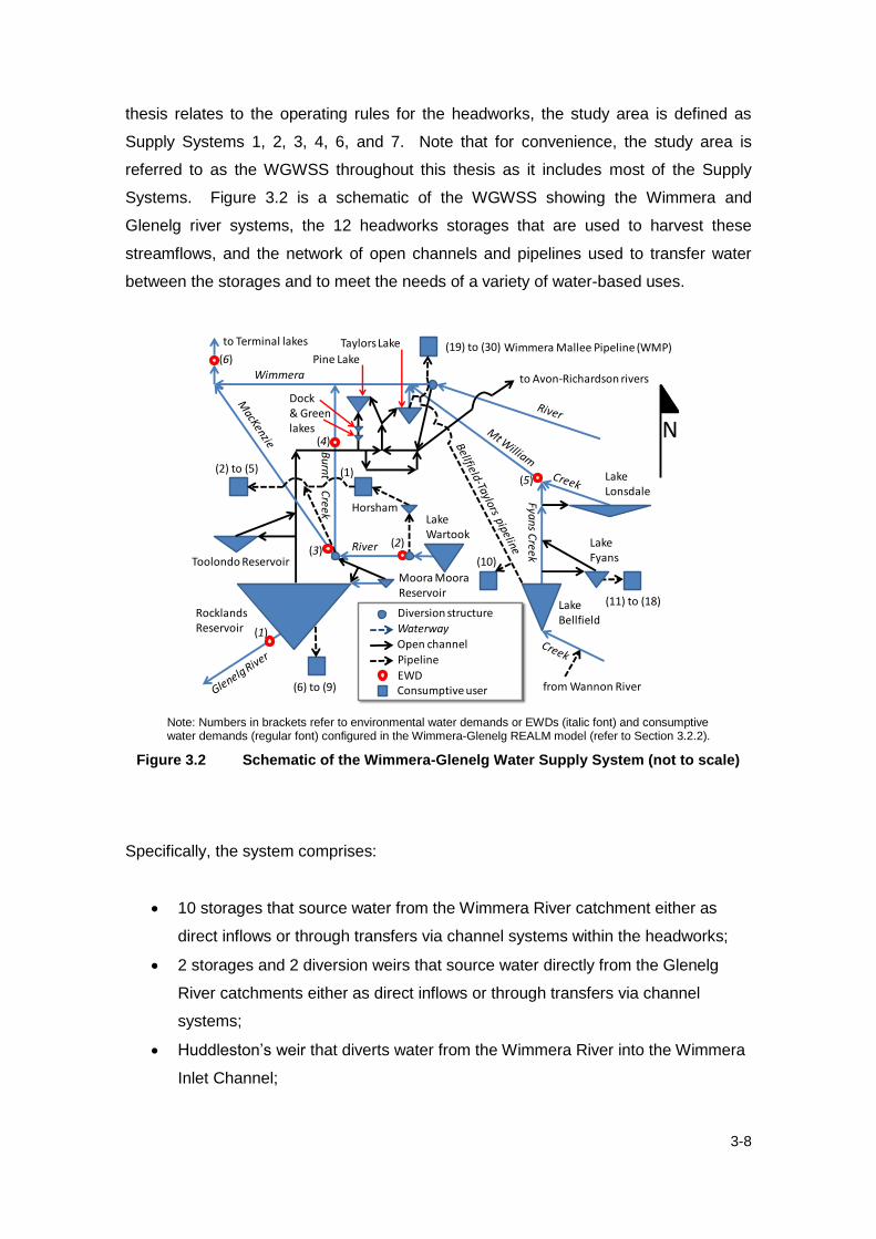
3-8
thesis relates to the operating rules for the headworks, the study area is defined as
Supply Systems 1, 2, 3, 4, 6, and 7. Note that for convenience, the study area is
referred to as the WGWSS throughout this thesis as it includes most of the Supply
Systems. Figure 3.2 is a schematic of the WGWSS showing the Wimmera and
Glenelg river systems, the 12 headworks storages that are used to harvest these
streamflows, and the network of open channels and pipelines used to transfer water
between the storages and to meet the needs of a variety of water-based uses.
Note: Numbers in brackets refer to environmental water demands or EWDs (italic font) and consumptive water demands (regular font) configured in the Wimmera-Glenelg REALM model (refer to Section 3.2.2).
Figure 3.2 Schematic of the Wimmera-Glenelg Water Supply System (not to scale)
Specifically, the system comprises:
10 storages that source water from the Wimmera River catchment either as
direct inflows or through transfers via channel systems within the headworks;
2 storages and 2 diversion weirs that source water directly from the Glenelg
River catchments either as direct inflows or through transfers via channel
systems;
Huddleston’s weir that diverts water from the Wimmera River into the Wimmera
Inlet Channel;
Pipeline
EWD
Diversion structure
to Terminal lakes
to Avon-Richardson rivers
Open channel
Consumptive user
(11) to (18)
Lake Fyans
Lake Lonsdale
Waterway
Lake Bellfield
HorshamLake Wartook
Rocklands Reservoir
Moora MooraReservoir
(6) to (9)
Toolondo Reservoir
Pine Lake
Taylors Lake
(2) to (5)
(10)
(1)
(19) to (30)Fya
ns C
reek
Wimmera
RiverB
urnt Creek
Dock& Green lakes
(2)
(6)
(5)
(1)
(4)
(3)
from Wannon River
Wimmera Mallee Pipeline (WMP)
N

3-9
Dad and Dave weir that diverts water from the MacKenzie River into Mt Zero
Channel for supply to Horsham;
A network of open channels and pipelines that transfer water between storages;
and
the Wimmera Mallee Pipeline which distributes water from the headworks to
Supply Systems 1, 2, 3, and 4 for watering of stock and for domestic, urban and
industrial consumption.
The headworks storages (summarised in Table 3.1) and the extensive distribution
network are operated as a single water resource system (with many possible
combinations of operating rules) to meet the needs of a variety of water-based uses.
Table 3.1 Headworks storages in the WGWSS (as in Wimmera-Glenelg REALM model)
River
basin Headworks storages
Full Supply Volume
(ML)
Full supply level to
Australian height datum
(metres)
Wimmera
Lake Bellfield 76,000 276.50
Lake Fyans 18,460 203.79
Lake Lonsdale 65,000 187.62
Taylors Lake 33,700 144.61
Lake Wartook 29,360 441.69
Horsham storages 328 310.10
Toolondo Reservoir 92,430 164.91
Dock Lake* 5,900 134.02
Green Lake* 5,350 135.70
Pine Lake* 64,200 143.89
Glenelg Moora Moora Reservoir 6,300 219.95
Rocklands Reservoir 348,000 195.47
* These storages are not for water supply purposes
Note that whilst Dock Lake, Green Lake, and Pine Lake are not operated for supply of
water to entitlement holders, these storages continue to be operated for other uses
such as for recreation and for flood mitigation purposes.

3-10
3.2.2 The Wimmera-Glenelg REALM model
The origins of the simulation model developed for this thesis begin with a REALM
model provided by the Department of Environment, Land, Water and Planning
(DELWP) in 2010 (pers. comm. Michael Finger). The DELWP identified this model, or
system file as it is referred to in REAL , as the “W PP2104.sys file.” Over the last 20
years of its development, the WMPP2104.sys file (and its predecessors) have been
used in numerous simulation modelling studies largely for the purposes of supporting
strategic long term planning processes (Godoy Consulting, 2014). In recent times, this
high quality simulation model was endorsed by the Murray-Darling Basin Authority as
part of its model accreditation process under the Murray-Darling Basin Plan (MDBA,
2011). More recently a review of the operation of the WGWSS was undertaken using
the simulation model to test the effectiveness of the current operating rules against
stakeholders’ storage management objectives (GW Water, 2014). It is worth
highlighting that researchers generally agree that the use of trusted simulation models
would have the potential of giving stakeholders and DMs greater confidence in O-S
modelling results (Maier et al., 2014).
As part of the process of setting up the O-S model (which is described in Section 3.4),
it was discovered that modifications to the WMPP2104.sys file were required in order
for it to connect to the optimisation engine and to improve its capability of searching for
candidate optimal operating plans. For this purpose, a lower-fidelity physically based
surrogate model was developed based on the original simulation model (i.e. the
WMPP2104.sys file). This surrogate model is referred to as the “Wimmera-Glenelg
REAL model” in this thesis. Razavi et al. (2012) described this type of surrogate
model as one that is (physically) based on the original simulation model preserving the
main functionality; but is less detailed. Refer to Section 3.4.1.1 for further details
regarding the benefits of using a lower-fidelity physically based surrogate model in
higher order MOOPs. Figure 3.3 shows the Wimmera-Glenelg REALM model as seen
through the graphical editor window in the REALM software package. This graphical
representation is very similar to the schematic of the WGWSS shown in Figure 3.2,
albeit with much greater detail. For the reader’s convenience, the headworks storages
of the WGWSS are noted in Figure 3.3.

3-11
Figure 3.3 The Wimmera-Glenelg REALM model
The Wimmera-Glenelg REALM model together with the input data representing
streamflows, rainfall, evaporation, and water demands are collectively referred to as a
model “scenario” or “run” in this thesis. In addition to the model containing the physical
representation of the WGWSS, it also includes all the key operating rules that regulate
water throughout the system. These modelled operating rules are collectively referred
to as an “operating plan” in this thesis. The operating plan embedded in the
WMPP2104.sys file represents the current practice in the WGWSS. This operating
plan was configured in the Wimmera-Glenelg REALM model and is referred to as the
“base case operating plan” and the model run is referred to as the “base case scenario”
throughout this thesis. It is important to highlight that the base case scenario is a
simulation-only run and that it is used for the purposes of providing a point of reference
in the analysis of the optimal operating plans found by the O-S model. For this
purpose, the base case scenario is run using one of the following hydro-climatic
conditions which are more fully described in Section 3.4.1.2.1:
Headworks storages
1. Lake Bellfield2. Lake Fyans3. Lake Lonsdale4. Taylors Lake5. Lake Wartook6. Horsham storages7. Toolondo Reservoir8. Dock Lake9. Green Lake10. Pine Lake11. Moora Moora Reservoir12. Rocklands Reservoir
1
2
3
4
5
6
7
8
9 10
1112

3-12
historic hydro-climatic conditions;
low to medium level GHG emissions; or
medium to high level GHG emissions.
With exception of the hydro-climatic input data above, all the modelling scenarios
presented in this thesis (i.e. the base case scenarios and the O-S scenarios) have the
same model specifications as follows:
a choice of two planning periods, viz. January 1891 to June 2009 for historic
hydro-climatic runs or January 2000 to December 2099 for future GHG
emissions;
monthly time-step;
environmental demands representing passing flow rules and prioritised water
flow requirements (refer to Section 3.2.3.1); and
consumptive demands representing full utilisation of water entitlements (refer
to Section 3.2.3.3).
Note that unlike the environmental and consumptive demands which are specified in
separate input data files, the interests for water in the WGWSS that have a social focus
(e.g. recreation) and those that affect all water users system-wide (e.g. water
allocations) are embedded in the operating rules of the Wimmera-Glenelg REALM
model. The reasons for this setup are explained in Section 3.2.3.2.
3.2.3 Stakeholders’ interests for water
Belton and Stewart (2002) describe multi-criteria decision making in water resource
planning studies as “mixed design and evaluation problems.” The authors explain that
such problems typically involve many stakeholders who are required to make in-depth
value judgements in relation to alternatives presented to them and that in practice
these comparative evaluations can only be performed on a relatively small number of
discrete options given the human cognitive load. In the context of this thesis, the
“design” stage generates a suitable shortlist of optimal operating plans for a detailed
“evaluation” by the D .

3-13
It is worth highlighting that for this thesis, there is a distinction made between those
whom have an interest for water and provide value judgements (i.e. stakeholders), and
those that have the ultimate decision-making power under law (e.g. DM). Based on a
recent Government-led planning study in the WGWSS, the key stakeholders were
water entitlement holders (i.e. water corporations and the Victorian Environmental
Water Holder) and the catchment management authorities (DSE, 2011). In that study,
the DM was the Minister for Environment, Climate Change and Water (“the inister”).
With respect to those planning studies led by water corporations and the Victorian
Environmental Water Holder, the key stakeholders are often community members that
encompass a wide range of interests and the DM is the water corporation or VEWH
(GWMWater, 2012a; 2012b; 2007; 2014; VEWH, 2013). However, in some of these
latter studies, the water corporation is in a sense a stakeholder advocate that uses the
value judgements of its customers to formulate its own institutional values in a
submission to the Minister (GWMWater, 2007; 2014). Importantly for this thesis, it is
assumed that the stakeholders and the DM are as per DSE (2011); the stakeholders
are the water entitlement holders and the catchment management authorities, and the
DM is the Minister. It is also worth pointing out that the above studies involved the use
of (REALM) simulation modelling outputs to support multi-criteria decision making
processes.
For the purposes of this thesis, the data collected as part of the above planning studies
in the WGWSS has been used in a desktop study to (i) identify stakeholders’ interests
for water in the WGWSS together with any relevant criteria by which to evaluate
candidate optimal operating plans; (ii) identify any relevant water management
planning decisions as part of the formulation of the MOOP; and (iii) postulate
stakeholders’ judgement values in relation to the selection of a preferred optimal
operating plan from a Pareto front (refer to Section 5.3).
As part of this desktop study, the various interests for water identified in the WGWSS
have been categorised into four major groups i.e. environmental, social, consumptive,
and those that affect all users system-wide. In recognition of the importance of
properly identifying interests and values in the water planning decision-making process
(Mooney et al., 2012), these four major interests for water are presented in
Sections 3.2.3.1 to 3.2.3.4 and serve as the basis of the conflicting objectives of the
higher order MOOP for the WGWSS.

3-14
3.2.3.1 Environmental
The environmental water within the WGWSS is held in trust by the Victorian
Environmental Water Holder and the Commonwealth Environmental Water Holder
(VEWH, 2014):
The Victorian Environmental Water Holder’s environmental water holding consists of:
41,560 ML/year of high reliability regulated water available from any storage
within the headworks system subject to water availability in the WGWSS;
passing flows of a lower reliability at five locations including the Glenelg River at
Rocklands Reservoir, Wimmera River at Huddlestons Weir, Mt William Creek at
Lake Lonsdale, Fyans Creek at Stawell Diversions Weir and the Wannon River
at Wannon Diversion; and
storage spills and any other catchment inflow that is not harvested by the
headworks system and extracted by private diversions.
The Commonwealth Environmental Water Holder’s environmental water holding
consists of 28,000 ML/year of high reliability regulated water subject to water
availability in the WGWSS. This entitlement originates from the sale of GW Water’s
irrigation water which became effective in the 2014-15 water year (VEWH, 2014). Note
that the Wimmera-Glenelg REALM model assumes that the 28,000 ML/year is
available to the environment as a low reliability allocation – refer to Section 3.2.3.4 for
further details.
The Victorian Environmental Water Holder (VEWH) performs this role in consultation
with waterway managers which in this case are the Glenelg-Hopkins and Wimmera
catchment management authorities. The waterway managers play the key role of
engaging with land managers, the storage operator (i.e. GWMWater), local landholders
and the community in the development of seasonal watering plans. The VEWH also
co-ordinates its efforts with other Australian jurisdictions including the Commonwealth
Environmental Water Holder (CEWH) and partners in the Living Murray Program. The
VEWH reports to the Minister and the DELWP has a role in advising the Minister of the
VEWH’s performance in meeting its objectives and functions as set out in Sections
33DA-33DZA of the Water Act 1989 (Vic).

3-15
The Seasonal Watering Plan 2014-15 sets out the environmental watering program for
all major river systems in Victoria including the Wimmera and Glenelg rivers (VEWH,
2014). With reference to the numbering scheme adopted in Figure 3.2, the following is
a summary of the key environmental assets for each of the six stream reaches
configured in the Wimmera-Glenelg REALM model:
1. Glenelg River – this reach is home to a number of important native fish
populations including river blackfish and a number of galaxid and pygmy perch
species. This reach also supports good riparian vegetation, including the
newly-discovered, endangered Wimmera bottlebrush (VEWH, 2014);
2. MacKenzie River (upper) – this is the only reach in the Wimmera basin that
contains populations of platypus and all endemic fish species (VEWH, 2014);
3. MacKenzie River (lower) – this is the only reach in the Wimmera basin that
contains populations of the endangered Wimmera bottlebrush (VEWH, 2014);
4. Burnt Creek – there have been river blackfish recorded in great abundance in
this reach and the riparian zone is characterised by a River Red Gum over-
storey (Alluvium, 2013b);
5. Mt William Creek – this reach contains a large assemblage of native species
including Mountain Galaxias and the vulnerable Southern Pygmy Perch. The
riparian vegetation is in reasonable to good condition particularly in the upper
section where it borders the Grampians National Park (Alluvium, 2013b); and
6. Wimmera River – most of this reach has been declared a heritage river under
the Heritage Rivers Act 1992 (Vic) for its biological, cultural and recreational
values, particularly in association with the terminal lakes. Additionally, the weir
pools at Dimboola and Jeparit are of high social and recreational significance.
Lake Hindmarsh is the largest freshwater lake in Victoria and supports a
number of environmentally significant values, including River Red Gum and
Black Box communities. Lake Albacutya which is approximately 15 km
downstream of Lake Hindmarsh is a Ramsar listed wetland of international
conservation significance. It fills only intermittently when Lake Hindmarsh
overflows. Both lakes support about 50 species of waterbird including the
endangered Great Egret and Freckled Duck. This reach contains other
important values including populations of freshwater catfish and endemic fish
such as the Flathead Gudgeon and Australian Smelt and a stocked population
of introduced, but vulnerable Golden Perch, Silver Perch and Freshwater

3-16
Catfish. The upper section of this reach borders Little Desert National Park,
where the uncleared bushland supports a floodplain and riparian zone in
excellent condition (Alluvium, 2013b).
The environmental flow requirements of the above stream reaches were quantified as
part of a freshwater ecological study (Alluvium, 2013a; 2013b). These flow
requirements are configured in the Wimmera-Glenelg REALM model as separate
environmental water demands (EWDs) in order to provide for the required flows (refer
to Figure 3.2). Unregulated or run-of-river flows are used in the first instance to meet
EWDs followed by regulated flows if there is any residual demand (GHD, 2011). In this
case, a criterion that could be used to evaluate candidate optimal operating plans with
respect to EWDs, would be the difference between the amount that is required at a
particular location (i.e. demand) and the amount that is provided to that location (i.e.
supply). This difference in the demand and supply at any given location is referred to
as a “flow deficit” in this thesis, or “environmental flow deficit” to be precise. Such
criteria together with the performance metrics in Section 3.2.4 are incorporated in the
formulation of the higher order MOOP by way of objective functions, to (refer to
Section 3.3.1).
3.2.3.2 Social
3.2.3.2.1 Recreation
Social interests for water in terms of recreation are significant in the WGWSS and vary
widely. For instance, boating and skiing enthusiasts require a safe minimum water
level to ensure that they do not hit underwater obstacles (e.g. tree stumps), while
others prefer to have a wide sandy berm for sand play by young children. In fact water-
based recreational activities are so plentiful in the WGWSS that industries have
emerged to cater for the large number of visitors to such activities. These tourism
enterprises are important in the WGWSS for socio-economic reasons, contributing to
the economy and generating employment. This section focuses on the recreation
amenity provided at Lake Lonsdale and Lake Fyans based on two recent planning
studies undertaken by GWMWater (2012a; 2012b).
GWMWater (2012a) points out that the primary role of Lake Lonsdale is as a source of
environmental water for the WGWSS, and that providing for recreation amenity at the
storage is a secondary goal. Recreational activities at Lake Lonsdale include

3-17
picnicking, walking, camping, fishing, canoeing, swimming, boating, skiing and sailing.
GWMWater (2012a) states that it was estimated that the contribution of Lake Lonsdale
to the local and regional economy was about $1.6 million annually in direct and indirect
benefits based on indicative visitor numbers. According to GWMWater (2012a), the
minimum desirable level beyond which recreation amenity is much reduced is at
1.5 metres or 5,379 ML in storage.
Lake Fyans is used by those living in Stawell, Ararat and the wider western district for a
range of water based recreation including fishing, swimming, powered and non
powered boating and sailing, water skiing, bird watching, duck shooting, and non-water
based pursuits such as bush walking and bike riding. GWMWater (2012b) states that
the fishing scouting, sailing, water skiing, swimming and holiday park patronage directly
contributed in excess of $7.8 million to the local economy in 2011. It estimated that the
employment generated by that economic input was about 95 full-time equivalent jobs
and that this contributed to more than $23.3 million annually. According to GWMWater
(2012b), a suitable minimum water level for recreation is 1.5 metres or 1,761 ML in
storage.
Moreover, one lobby group has focused on the importance of recreation in terms of the
social well-being of communities in the WGWSS (The Wimmera Mail-Times, 2013b;
2013c). The Natimuk Lake Action Group asserts that the recent review of the
operation of the WGWSS by GWMWater (2014) did not adequately address recreation
interests because it did not consider the mental and physical health of people in the
WGWSS, particularly the younger generation whom it claims did not have many
healthy recreation options at that time.
GWMWater holds an entitlement for recreation of 2,590 ML/year subject to water
availability in the WGWSS. Whilst this represents a small proportion of the total
entitlement volume in the WGWSS (i.e.
), recreation amenity is also
provided by water held in storage. GWMWater (2012) explains that the operator has
limited discretion to move water around the WGWSS for meeting recreation needs
only. Instead, the operator provides different types of recreation amenity by changing
certain operating rules within the operating plan. In this case, a criterion that would be
used to evaluate candidate optimal operating plans with respect to recreation at Lake
Lonsdale and Lake Fyans is the volume held in those storages. Such criteria together

3-18
with the performance metrics in Section 3.2.4 are incorporated in the formulation of the
higher order MOOP by way of objective functions, to (refer to Section 3.3.1).
3.2.3.2.2 Cultural
As for the recreation-based social interests for water described in Section 3.2.3.2.1,
this section focuses on the cultural values that exist at Lake Lonsdale and Lake Fyans
based on the same planning studies undertaken by GWMWater (2012a; 2012b). Lake
Lonsdale and Lake Fyans have been mapped as an area of cultural heritage sensitivity
under the Aboriginal Heritage Act 2006 (Vic). The two Traditional Owner Groups in the
region are the Gunditj Mirring and the Barengi Gadjin Land Council.
According to Emsconsultants (2009), little is known of the cultural values associated
with the Lake Fyans storage area given that it has not been surveyed for aboriginal
occupation. However, as Lake Lonsdale has been surveyed for aboriginal occupation,
more is known of the cultural connection it has with indigenous people. For instance,
when Lake Lonsdale is not empty it has been documented that it protects a number of
burial sites on the storage bed. The largest of these archaeological deposits occurs
across the north eastern part of the storage. Moreover, a study undertaken by
Emsconsultants (2009) as part of the Western Region Sustainable Water Strategy
(DSE, 2011) reveals that indigenous people are critical of non-indigenous water
resource management. This is mainly due to indigenous people having a different view
on water and a belief that it is inextricably related to the land, playing a significant role
in traditional and cultural practice. According to Emsconsultants (2009), indigenous
people observed burial sites being damaged during the period 1997 to 2010 by cars
being driven across the dry (Lake Lonsdale) storage bed and by farmers grazing their
stock over it. Another criticism highlighted by Emsconsultants (2009), is that
indigenous people were not consulted in the Victorian Government’s conversion of
rights to water to bulk water entitlements in the WGWSS.
Emsconsultants (2009) lists the following sites within the WGWSS as having cultural
significance:
all waterfalls and underground water in the Grampians National Park which
indigenous people refer to as Gariwerd. (Note that the WGWSS headworks are
located in and around the Grampians National Park);
Yarriambiack Creek (a tributary of the Wimmera River);

3-19
all wetlands of the upper Glenelg River (upstream of Rocklands Reservoir);
the many waterways in the region which have the highest concentration of scar
trees in Australia;
Toolondo Creek (a stream which runs into Toolondo Reservoir); and
McKenzie Creek.
The criterion that would be used to evaluate candidate optimal operating plans with
respect to cultural values at Lake Lonsdale is the volume held in storage. However, as
the desired recreation amenity at Lake Lonsdale requires a volume that is greater than
that for cultural purposes, the criterion for recreation interests for water described in
Section 3.2.3.2.1 will also suffice for cultural purposes. Similarly, it is anticipated that
the provision for recreation amenity at Lake Fyans would go some way to protect the
cultural heritage associated with that storage area.
3.2.3.2.3 Water quality
As operator of the WGWSS, GWMWater is responsible for operating the WGWSS to
supply entitlement holders with water that is fit for purpose. It does this by operating to
a set of water quality targets for each storage (e.g. salinity, turbidity etc) with due
consideration to any exceptional circumstances (e.g. bushfire, flooding etc). However
as the Wimmera-Glenelg REALM model is not setup to account for such water quality
parameters, this thesis focuses on the (storage) operation of the WGWSS in so far as
managing water quality is concerned. Whilst all storages in the WGWSS have
operating rules associated with maintenance of water quality, Rocklands Reservoir is
presented given that it is the largest and arguably the most important storage in the
system.
In addition to Rocklands Reservoir being an important source of water to the Glenelg
River, it also supports the entire system by holding the majority portion of carryover
water, reserve for following year, and water to consumptive users. During times when
Rocklands Reservoir is relatively low the salt level becomes elevated. Historically, it
has been observed that dry periods can have the effect of accumulating salt and
nutrients and that high inflows can result in high levels of colour. This is of particular
concern to a consumptive user (i.e. Wannon Water – refer to Section 3.2.3.3) which is
dependent on Rocklands Reservoir; requiring water from Rocklands Reservoir to be

3-20
mixed with water sourced from its local diversions (which are often of better quality) in
order to achieve an acceptable salt level. According to GWMWater (2011), the
strategy for maintaining water quality within Rocklands Reservoir is: (i) the continued
turn-over of large volumes of water which coincides with the delivery of environmental
passing flows as inflows occur; and (ii) a minimum desirable level of 189.06 m
Australian Height Datum (AHD) or 69,600 ML in storage. This minimum operating level
assists to manage water quality, particularly salinity levels, by buffering poor quality
inflows during low inflow years. Additionally, this minimum operating level provides
some recreation amenity (GWMWater, 2011).
In this case, the criterion that would be used to evaluate candidate optimal operating
plans with respect to the management of water quality at Rocklands Reservoir is the
volume held in storage. Such criteria together with the performance metrics in
Section 3.2.4 are incorporated in the formulation of the higher order MOOP by way of
objective functions, to (refer to Section 3.3.1).
3.2.3.3 Consumptive
Consumptive use in the WGWSS is managed by GWMWater, Wannon Water and
Coliban Water. These government-owned water corporations are established under
Section 85 of the Water Act 1989 (Vic) and must provide, manage, operate and protect
water supply and sewerage systems for urban customers including collection, storage,
treatment, transfer and distribution functions as required. In addition to operating the
WGWSS, GWMWater holds an entitlement for 81,570 ML/year and supplies water to
approximately 52,000 urban properties in 71 towns and 11,000 rural customers,
provides wastewater services to 26 towns, and supplies reclaimed water to 39 end
users (GWMWater, 2012c). Wannon Water holds an entitlement of 2,120 ML/year and
sources its water directly from Rocklands Reservoir to supply Balmoral and to
supplement supplies to the townships of Hamilton and Cavendish located in the
Glenelg Basin (Wannon Water, 2012). Coliban Water holds an entitlement of 300
ML/year and sources its water directly from the Wimmera Mallee Pipeline (WMP) to
supply a residential population of 986 located in Wedderburn, Korong Vale, Borung and
Wychitella (Coliban Water, 2012). All three water corporations hold entitlements of
high reliability water, subject to water availability in the WGWSS.

3-21
All water corporations in Victoria (Australia) are required to prepare a Water Supply
Demand Strategy (WSDS) which sets out a 50-year strategy to balance the supply of
water to meet residential, business and community water needs (DSE, 2011). WSDSs
are reviewed every five years and are a key input into every corporation’s strategic
planning process. WSDSs set out a corporation’s long term level of service objectives
which may be considered in the context of this thesis, as consumptive user criteria.
Whilst these service objectives are system-specific, characterised by a particular
system’s supply and demand needs, there are common criteria employed to evaluate
candidate optimal operating plans with respect to supply consumptive demands as
follows:
Reliability of supply – a term used to indicate the frequency of restrictions.
Reliability is often expressed as the probability of years that water restrictions
will not be imposed (Erlanger and Neal, 2005). In this case, GWMWater and
the other two water corporations (i.e. Wannon Water and Coliban Water) have
agreed to provide urban customers with their respective unrestricted demand in
93% and 95% of years respectively, assuming historic hydro-climatic conditions
(GWMWater, 2012c; Wannon Water, 2012; Coliban Water, 2012).
Maximum restriction level – a term used to indicate the severity/duration of
restrictions. Wannon Water and Coliban Water have agreed to provide no
worse than stage 3 (out of 4) level of restrictions (but do not specify any
maximum duration of restriction (Wannon Water, 2012; Coliban Water, 2012).
GWMWater sets a minimum level of service in which it agrees to supply at least
50% of the unrestricted demand in years where restrictions are in force
(GWMWater, 2012c).
The Wimmera-Glenelg REALM model includes 30 separate consumptive demands for
reasons of accounting for water corporations’ demand type and source of supply (refer
to consumptive user (1) to (30) in Figure 3.2). Similar to the criterion for the
environment described in Section 3.2.3.1, a criterion that could be used to evaluate
candidate optimal operating plans with respect to consumptive demands, would be the
difference between the demand at a particular location and the amount supplied to that
location. This difference in the demand and supply at any given location is referred as
“consumptive user deficit” in this thesis. Such criteria together with the performance

3-22
metrics in Section 3.2.4 are incorporated in the formulation of the higher order MOOP
by way of objective functions, to (refer to Section 3.3.1).
3.2.3.4 System-wide
An interest for water that was raised by most stakeholders was the water allocations in
the WGWSS, specifically the “reliability” of full water allocations. The reason for this is
due to the fact that the supply to all water users is affected by these water allocations.
The Wimmera-Glenelg bulk water entitlements specify each entitlement holders’ share
of the resource (or water allocation) subject to the available water in the WGWSS
(VGG, 2010). The available water in the WGWSS is defined as the total volume of
water available for allocation to all entitlement holders. Table 3.2 shows that at any
given volume of “Water Available”, an entitlement holder has a pre-defined (volumetric)
share of that volume of water.
Table 3.2 Shares of Water Available (source: VGG, 2010)

3-23
Table 3.3 provides the method for estimating the Water Available in the WGWSS. The
above shares of Water Available (Table 3.2) and calculation of Water Available (Table
3.3) are configured in the Wimmera-Glenelg REALM model. It is important to note the
following model assumptions with regards to these computations which are consistent
with DELWP’s REAL model, W PP2104.sys (refer to Section 3.2.2):
Grampians Wimmera allee Water’s (i.e. GW Water’s) 28,000 ML irrigation
allocation (i.e. 9,000 ML “irrigation losses” plus 19,000 ML “irrigation product”) is
available to the environment as a low reliability allocation in recognition of the
water entitlement purchased by the environment. Therefore, the total system
water allocation in column A of Table 3.2 is 97,550 ML (i.e. 125,550 ML less
28,000 ML).
The measured total volume in store at the start of month i is the sum of the
modelled volume held in Rocklands Reservoir, Taylors Lake, Toolondo
Reservoir, Lake Bellfield, Moora Moora Reservoir, Lake Lonsdale, Lake
Wartook, and Lake Fyans. “ onth i” refers to each month of the water
accounting year, beginning 1 July and ending 30 June.
The estimate of total dead storage is 11,000 ML.
The volume of carryover is zero. Note that this means that the level of
development is assumed to represent full uptake of entitlement.
An estimate of harvestable inflows and pick-up from start of month i to 30 June
next is nil. Note that this is quite conservative as it assumes that there will be
no inflows to the WGWSS throughout the year.
The measured total amount of water released from headworks from 1 July last
to the start of month i is the sum of all the releases as calculated by the model,
at each monthly time-step.
The volume of reserve is subject to the prevailing available water as given in
GHD (2011).
The estimated headworks losses from the start of month i to 30 June next is
subject to the sum of the volume held in the storages specified in the second
bullet point above as per GHD (2011).

3-24
Table 3.3 Method for estimating Water Available in the WGWSS (VGG, 2010)
ote: “ onth i” refers to each month of the water accounting year beginning 1 July and ending 30 June
In this case, the criterion that would be used to evaluate candidate optimal operating
plans with respect to system-wide interests for water is the total system water
allocation. Such criteria together with the performance metrics in Section 3.2.4 are
incorporated in the formulation of the higher order MOOP by way of objective functions,
to (refer to Section 3.3.1).
3.2.4 Performance metrics
From the discussion of stakeholders’ interests for water in Section 3.2.3, the following
criteria are suggested as a means to evaluate candidate optimal operating plans:
Environmental flow deficits of 6 EWDs representing environmental interests for
water (refer to Section 3.2.3.1);
Volume held in storage at Lake Lonsdale, Lake Fyans, and Rocklands
Reservoir representing social interests for water in terms of the provision for
recreation amenity at Lake Lonsdale and Lake Fyans and for the maintenance
of water quality at Rocklands Reservoir (refer to Section 3.2.3.2);
Consumptive user deficits of 30 consumptive user demands representing
consumptive interests for water (refer to Section 3.2.3.3); and
Total system water allocations for the WGWSS representing system-wide
interests for water (refer to Section 3.2.3.4).

3-25
For these criteria to be incorporated in the higher order MOOP, a suitable unit of
measure is required to evaluate candidate optimal operating plans on a quantitative
basis with respect to the four interests for water identified (i.e. environmental, social,
consumptive, and system-wide interests). These performance metrics ought to be
comprehensive and aimed at providing the basis for meaningful dialogue amongst the
stakeholders and the DM, as required by the planning process. For the purposes of
this thesis, it is assumed that the participants require the following information: (i) the
frequency of desirable or successful events (i.e. reliability); (ii) the rate of recovery of
the WGWSS after undesirable events or failures occur (i.e. resiliency), and (iii) the
severity of failures (i.e. vulnerability). It is worth highlighting that Sandoval-Solis et al.
(2011) makes reference to several other studies that show that these three
performance metrics summarise essential performance parameters in a meaningful
manner.
Sections 3.2.4.1 to 3.2.4.3 present these performance metrics (i.e. reliability, resiliency,
and vulnerability) in terms of an annual time-period (i.e. July to June) given that this is
the preferred basis on which to communicate such information to the community in the
WGWSS (DSE, 2011).
3.2.4.1 Reliability
Loucks (1997) defined reliability as the probability of successful events over the
planning period. In the case of environmental flow deficits (i.e. Section 3.2.3.1) and
consumptive user deficits (i.e. Section 3.2.3.3), a successful event is defined as a
period of ‘nil’ deficits. For each time period , deficits are positive when the
water demand is more than the water supplied to the th interest for water,
and when the water supplied is equal to the water demand deficits are
zero :
(3.2)
Time-based reliability may be expressed as the portion of time the water
demand is fully satisfied with respect to the number of time
intervals considered (McMahon et al., 2006). For this thesis, it is assumed that
annual environmental flow deficits ( ) and annual consumptive user deficits

3-26
( ) are required and so corresponds to the number of years over the
model planning period, from 1891 to 2009:
(3.3)
(3.4)
In the case of social interests for water (i.e. Section 3.2.3.2), a successful event is
defined as a period when the volume held in a storage is greater than the minimum
volume that provides the desired level of recreation amenity or water quality as
required. For each time period , time-based reliability would be expressed as the
portion of time the volume held in a storage was greater than the minimum desired
volume with respect to the number of time intervals considered. For this thesis, it is
assumed that monthly storage volumes are required for Lake Lonsdale ( ), Lake
Fyans ( ), and Rocklands Reservoir ( ) and so corresponds to the number of
months over the model planning period, from 1891 to 2009:
(3.5)
(3.6)
(3.7)
In the case of system-wide interests for water (i.e. Section 3.2.3.4), a successful event
is defined as a period when the total system water allocation is equal to the full
allocation of 97,550 ML. For each time period , time-based reliability would be
expressed as the portion of time the total system water allocation is equal to 97,550 ML
with respect to the number of time intervals considered. For this thesis, it is
assumed that the total system water allocation in June ) is required and so
corresponds to the number of years over the model planning period, from 1891 to
2009:
(3.8)

3-27
3.2.4.2 Resiliency
Agrell et al. (1998) defined resiliency as a system’s capacity to adapt to changing
conditions i.e. rate of recovery. This is particularly important given that climate
conditions are no longer steady. In recent times of prolonged dry conditions (1996 to
2010), storage levels in the WGWSS dropped to unprecedented levels and water
carting programs were required to deliver water to users as operating the system under
these extreme conditions would result in significant volumes of water lost through
seepage and evaporation (DSE, 2011). Hashimoto et al. (1982) described resiliency
as the probability that a system recovers from a period of failure. Sandoval-Solis et al.
(2011) defined resiliency as the probability of a successful period following a failure
period for all failure periods. In the case of environmental flow deficits (i.e.
Section 3.2.3.1) and consumptive user deficits (i.e. Section 3.2.3.3), the resiliency
would be the probability of ‘nil’ deficit periods following deficit periods with respect to all
deficit periods. As this thesis assumes that annual environmental flow deficits
( ) and annual consumptive user deficits (
) are required (refer
to Equations 3.3 and 3.4), resiliency is also expressed in terms of the number of years
that successful/failure periods occur over the planning period:
(3.9)
(3.10)
In the case of social interests for water (i.e. Section 3.2.3.2), a successful event is
defined as a period when the volume held in a storage is greater than the minimum
volume that provides the desired level of recreation amenity or water quality as
required. Therefore, a failure period is the reverse i.e. when the volume held in a
storage is equal to or less than the minimum desired volume. As this thesis assumes
that monthly storage volumes are required for Lake Lonsdale ( ), Lake Fyans ( ),
and Rocklands Reservoir ( ) (refer to Equations 3.5 to 3.7), resiliency is also
expressed in terms of the number of months that successful/failure periods occur over
the planning period:
(3.11)
(3.12)

3-28
(3.13)
In the case of system-wide interests for water (i.e. Section 3.2.3.4), a successful event
is defined as a period when the total system water allocation is equal to the full
allocation of 97,550 ML and a failure period is when the total system water allocation is
less than the full allocation. As this thesis assumes that the total system water
allocation in June ) is required (refer to Equation 3.8), resiliency is also
expressed in terms of the total system water allocation in June:
(3.14)
3.2.4.3 Vulnerability
Hashimoto et al. (1982) defined vulnerability as the likely value of failures, if they occur,
which effectively describes the severity of failures. High reliability may hide disastrous
consequences once a failure has occurred. Agrell et al. (1998) suggested that to
measure the severity of a failure, a numerical measure of the most severe outcome
during a failure state ought to be used. This has been expressed in a variety of ways
including the average failure, the average of maximum failures over all continuous
failure periods, and the probability of exceeding a certain failure threshold (Sandoval-
Solis et al., 2011). Sandoval-Solis et al. (2011) defined vulnerability as the sum of the
failures, divided by the number of times failures occurred. Dimensionless vulnerability
is calculated by dividing this average failure by the average of the water demand for
that particular interest for water (Sandoval-Solis et al., 2011). In the case of
environmental flow deficits (i.e. Section 3.2.3.1) and consumptive user deficits (i.e.
Section 3.2.3.3), the vulnerability would be the average deficit divided by the average
of the EWDs and consumptive user demands (respectively) over the planning period.
As this thesis assumes that annual environmental flow deficits and annual consumptive
user deficits are required (refer to Equations 3.3, 3.4, 3.9 and 3.10), vulnerability is also
expressed in terms of the number of years that deficits occur over the planning period:
(3.15)
(3.16)

3-29
In the case of social interests for water (i.e. Section 3.2.3.2), a failure event is defined
as a period when the volume held in a storage is equal to or less than the minimum
volume that provides the desired level of recreation amenity or water quality as
required. Therefore, vulnerability would be the average failure divided by the average
volume held in that storage over the planning period. As this thesis assumes that
monthly storage volumes are required for Lake Lonsdale ( ), Lake Fyans ( ), and
Rocklands Reservoir ( ) (refer to Equations 3.5 to 3.7, and 3.11 to 3.13),
vulnerability is also expressed in terms of the number of months that failure periods
occur over the planning period:
(3.17)
(3.18)
(3.19)
In the case of system-wide interests for water (i.e. Section 3.2.3.4), a failure event is
defined as a period when the total system water allocation is less than the full
allocation of 97,550 ML. As this thesis assumes that the total system water allocation
in June ) is required (refer to Equations 3.8 and 3.14), vulnerability is also
expressed in terms of the total system water allocation in June:
(3.20)
3.3 A higher order MOOP for the Wimmera-Glenelg Water Supply System
Having identified all the major interests for water in Section 3.2, a higher order MOOP
is formulated for the WGWSS in Section 3.3 with sustainability as an overall goal. The
problem is structured hierarchically using a value tree. Belton and Stewart (2002) state
that a value tree is often used in multi-criteria decision making problems to structure
the problem on a hierarchical basis with the broad interests towards the top of the tree
and the more specific criteria towards the bottom of the tree. For the purposes of this
thesis, Figure 3.4 presents the value tree of the higher order MOOP for the WGWSS.
For ease of presentation, the top of the tree is shown to the left of the figure and
corresponds to the highest level criteria, being in this case, the sustainability of the

3-30
WGWSS. The next criteria level down represents the four interests for water identified
(i.e. environmental, social, consumptive, and system-wide interests). The third criteria
level from the top represents a further clarification and/or breakdown from the four
interests for water of the second level.
Note: ‘ ’ refers to the mth objective function which is defined in Section 3.3.1
Figure 3.4 Value tree of the higher order MOOP for the WGWSS
For instance, environmental interests for water are expressed in terms of
environmental flow deficits at 6 locations and social interests for water are expressed in
terms of minimum storage levels for recreation amenity and also maintenance of water
quality. The lowest level criteria, or the bottom of the tree, is shown to the right of the
figure and represents the underlying conflicts of the problem and are unambiguous and
measurable (Belton and Stewart, 2002; Juwana et al., 2012). In this case, the higher
order MOOP is structured so that the lowest level criteria represent 18 conflicting
objective functions, to (refer to Equations 3.21 to 3.38).
Minimum water level at Lake Lonsdale (f5 - Eq 3.25)
Minimum water level at Lake Fyans (f8 - Eq 3.28)
Minimum water level at Rocklands Reservoir (f11 - Eq 3.31)
Environmental flow deficits at 6 locations (f2 - Eq 3.22)
Total water allocation (f17 - Eq 3.37)
Minimum storage levels for recreation amenity
Minimum storage levels for maintenance of water quality
Consumptive user deficits of 30 user groups (f14 - Eq 3.34)
Social interests to water
(Section 3.2.3.2)
Sust
ain
abili
ty o
f WG
WSS
Environmental interests to water
(Section 3.2.3.1)
Environmental flow deficits at 6 locations (f3 - Eq 3.23)
Environmental flow deficits at 6 locations (f1 - Eq 3.21)
Total water allocation (f18 - Eq 3.38)
Total water allocation (f16 - Eq 3.36)
Consumptive user deficits of 30 user groups (f15 - Eq 3.35)
Consumptive user deficits of 30 user groups (f13 - Eq 3.33)
Minimum water level at Rocklands Reservoir (f12 - Eq 3.32)
Minimum water level at Rocklands Reservoir (f10 - Eq 3.30)
Minimum water level at Lake Lonsdale (f4 - Eq 3.24)
Minimum water level at Lake Lonsdale (f6 - Eq 3.26)
Minimum water level at Lake Fyans (f7 - Eq 3.27)
Minimum water level at Lake Fyans (f9 - Eq 3.29)
Environmental flow deficits at 6 locations
Consumptive interests to water
(Section 3.2.3.3)
Consumptive user deficits of 30 user groups
System-wide interests to water
(Section 3.2.3.4)
Total water allocation

3-31
It is worth highlighting that formulating a higher order MOOP using higher criteria levels
(e.g. the four interests for water) would have the effect of reducing the dimensionality of
the problem whereas lower criteria levels (e.g. the 18 objective functions) would have
the reverse effect. Extending this concept to the development of a sustainability index
is an important step in the development of a structured procedure for the multi-
objective optimisation of complex water resource systems.
3.3.1 Objective functions
With reference to the mathematical expression for a MOOP given in Equation 3.1, the
aim in solving the higher order MOOP for this thesis is to find a set of operating rules
which minimise/maximise all the objective functions (simultaneously) and which satisfy
the constraints of the problem. These objective functions play a role of guiding the
optimisation search towards candidate optimal operating plans that perform the best in
terms of the values of these objective functions. Moreover, the higher order MOOP for
this thesis is structured so that there is a link between the conflicting interests for water
in the WGWSS and the optimisation search as given by the value tree of the MOOP in
Figure 3.4. The 18 objective functions of the higher order MOOP for this thesis are
provided in Equations 3.21 to 3.38. Note that in each case, the time period ( ) refers to
each month from July to June in line with the water accounting year used in the
WGWSS (VGG, 2010).
The 18 objective functions are formulated using the 18 performance metrics presented
in Section 3.2.4; with sustainability as an overall goal. The sustainability of the
WGWSS is measured in terms of maximising the reliability ( ), maximising the
resiliency ( ), and minimising the vulnerability ( ) of the th interest for water. It is
worth highlighting that further to the conflicts that exist amongst the four interests for
water (i.e. environmental, social, consumptive, and system-wide interests), additional
conflicts arise within these individual interests for water. For instance, increasing the
performance of the environmental objectives means that there is less water extracted
from waterways which reduces the volume available for supply to consumptive users
and for provision of recreation amenity, and vice versa. Additionally, within the
environmental interests for water, an increase the reliability of nil environmental flow
deficits does not necessarily equate to an increase in resiliency; nor does the increase
in any or both of these two objectives (i.e. reliability and resiliency) result in reduced
vulnerability of such deficits, and vice versa.

3-32
3.3.1.1 Environmental
For the criteria in Figure 3.4 representing environmental interests for water, the
corresponding objective functions, to , (Equations 3.21 to 3.23) are based on
performance metrics (Equation 3.3), (Equation 3.9), and
(Equation 3.15) respectively:
(3.21)
(3.22)
(3.23)
3.3.1.2 Social
For the criteria in Figure 3.4 representing social interests for water, the corresponding
objective functions, to (Equations 3.24 to 3.32) are based on performance
metrics (Equation 3.5), (Equation 3.11), (Equation 3.17),
(Equation 3.6), (Equation 3.12), (Equation 3.18), (Equation 3.7),
(Equation 3.13), and (Equation 3.19) respectively:
, (3.24)
(3.25)
(3.26)
, (3.27)
(3.28)
(3.29)
, (3.30)
(3.31)
(3.32)

3-33
3.3.1.3 Consumptive
For the criteria in Figure 3.4 representing consumptive interests for water, the
corresponding objective functions, to (Equations 3.33 to 3.35) are based on
performance metrics (Equation 3.4), (Equation 3.10), and
(Equation 3.16) respectively:
, (3.33)
(3.34)
(3.35)
3.3.1.4 System-wide
For the criteria in Figure 3.4 representing system-wide interests for water, the
corresponding objective functions, to (Equations 3.36 to 3.38) are based on
performance metrics (Equation 3.8), (Equation 3.14), and
(Equation 3.20) respectively:
, (3.36)
(3.37)
(3.38)
3.3.2 Decision variables
With reference to the mathematical expression for a MOOP given in Equation 3.1, the
aim in solving the higher order MOOP for this thesis is to find decision variable values
that satisfy the constraints of the problem and which minimises/maximises all the
objective functions, simultaneously. For this thesis, it is assumed that the decision
variables for the higher order MOOP are expressed in terms of 24 water management
planning decisions representing the key operating rules which control and regulate the
water resources within the WGWSS. The planning decisions are categorised into six
areas of system operation, viz.; (i) priorities of supply between different sources of
supply and between different user groups; (ii) a storage flood reserve volume to
provide flood attenuation; (iii) environmental allocation shares for apportioning

3-34
environmental water allocations between river basins; (iv) the preference of alternative
flow paths for the harvesting and/or transfer of water; (v) storage maximum operating
volumes for the key water harvesting storages; and (vi) storage draw down priorities
and storage targets. Table 3.4 provides a summary of the 24 water management
planning decisions which collectively are referred to as an “operating plan” in this
thesis.
Table 3.4 Water management planning decisions for the WGWSS
Category Decisions Value range
Priority of supply
Should Moora Moora Reservoir be the first priority of
supply or Lake Wartook to demands (2) to (5) and EWDs in MacKenzie River (3) and Burnt Creek (4)?
Either Lake Wartook or Moora Moora Reservoir is first priority and the other is a
supplementary source of supply
Should Horsham (1) be supplied in preference to the EWD
in MacKenzie River at Dad and Dave Weir (2) or vice versa?
Either Horsham (1) or EWD (2) is satisfied first
Should water be harvested into Taylors Lake in preference to meeting the EWD in MacKenzie River (3) or vice versa?
Either harvest flows into Taylors Lake or EWD (3) is satisfied first
Should water be harvested into Taylors Lake in preference
to meeting the EWD in Burnt Creek (4) or vice versa? Either harvest flows into Taylors Lake or
EWD (4) is satisfied first
Should consumptive demands (6) to (9) be satisfied before
the EWDs in Glenelg River (1) or vice versa? Either consumptive demands (6) to (9) or
EWD (1) is satisfied first
Should water be harvested into Wimmera Inlet Channel
(WIC) in preference to meeting passing flows in Wimmera River at Huddlestons Weir or vice versa?
Either harvest flows into WIC or provide passing flow first
Should water be held in storage for supply to consumptive
demands (19) to (30) in preference to the EWD in Mt William Creek at Lake Lonsdale (5) or vice versa?
Either hold water in Lake Lonsdale for consumptive demands (19) to (30) or supply
EWD (5) first
Flood reserve volume
How much flood reserve should be provided at Lake
Wartook over the period April to September? Either hold no reserve or hold a maximum of
up to the full storage capacity in June
Share of environ-mental
allocation
How much of the environmental water allocation should be
released in the Glenelg River basin? Either no share or up to 100% of the
environmental water allocation
How much of the environmental water allocation should be
released in the Wimmera River basin at Lake Wartook?
Either no share or up to the remaining share of the environmental water allocation after that provided for the Glenelg River basin
How much of the environmental water allocation should be released in the Wimmera River basin at Lake Lonsdale?
Either no share or up to the remaining share of the environmental water allocation after
that provided for the Glenelg River basin and that at Lake Wartook
Flow path
Should Mt William Creek flows be harvested into Wimmera Inlet Channel or should all these flows be passed down to
Wimmera River?
Either harvest flows into Wimmera Inlet Channel or pass all flows to Wimmera River
Should water from Lake Bellfield be mixed with water from
Taylors Lake via the Bellfield-Taylors Pipeline?
Supply from Lake Bellfield may result in one of three outcomes; nil, a proportion based on
the volume in storage, or 100%
Storage maximum operating volume
Toolondo Reservoir 0 to 92,430 ML
Lake Lonsdale Inlet is either open or closed
Lake Bellfield 0 to 76,000 ML
Taylors Lake 0 to 33,700 ML
Rocklands Reservoir 0 to 348,000 ML
Lake Lonsdale 0 to 65,000 ML
Moora Moora Reservoir 0 to 6,300 ML
Storage draw down
priority and
storage target
What should be the drawdown priority of the headworks
storages? Each storage is assigned a unique draw
down priority from 1 to 8
What should be the second point on the target curve for
the headworks storages? Any volume between dead storage and FSL
What should be the third point on the target curve for the
headworks storages? Any volume between the second target point
and FSL
What should be the fourth point on the target curve for the
headworks storages? Any volume between the third target point
and FSL
‘ ’ refers to decision variable which are defined in Section 3.3.2. ‘EWDs’ refers to environmental water demands. Number in brackets refers to consumptive user demand centres and environmental flow sites shown in Figure 3.2.

3-35
Each sub-section under Section 3.3.2 presents the six categories of system operation
in terms of the mathematical equations that are configured in the Wimmera-Glenelg
REALM model. The Wimmera-Glenelg REALM model consists of nodes representing
diversion structures, reservoirs, and water demands which are connected with carriers
which represent waterways, channels and pipes within the WGWSS (refer to Figure
3.3). In REALM, the preferred flow distribution is determined by user-defined penalties
in the carriers. When there is a choice of flow paths, the carrier with the lowest penalty
will transfer flow up to the user-specified capacity, then the carrier with the next higher
penalty will be used and so on until the demand for water at the downstream node is
satisfied. A wide range of operating rules can be configured in the model by using
variable capacity carriers in which mathematical equations are expressed in terms of
an x-y relationship, where y represents the capacity of the carrier at a given simulation
time-step and x is a function of any number of system variables such as carrier
flow/capacity, water demand, and reservoir volume etc. Alternatively the user can
exploit the functional attributes of the nodes and carriers within the model to represent
more conventional rules/constraints such as a minimum flow carrier capacity
representing environmental minimum flow requirements in a waterway. Further details
regarding the operation of REALM is provided in Section 2.2.4.1. Note that words in
upper case font refer to node and carrier names within the Wimmera-Glenelg REALM
model.
3.3.2.1 Priority of supply
There are seven planning decisions regarding the priority of supply between different
sources of supply and between different user groups within the WGWSS. With the
exception of (Equation 3.39) which relates to the priority of supply between
different sources of supply, to (Equations 3.40 to 3.45) relate to the priority of
supply between different user groups.
a) Should Moora Moora Reservoir be the first priority of supply or Lake Wartook to
demands (2) to (5) and EWDs in MacKenzie River (3) and Burnt Creek (4)?
Carrier MACKENZIE RIV U represents the MacKenzie River reach between
EWDs (2) and (3) as shown in Figure 3.2. This carrier is used to set the priority
of supply between water that is available from Moora Moora Reservoir and Lake
Wartook for supply to consumptive demands (2) to (5) and EWDs (3) and (4).
When the penalty of MACKENZIE RIV U is equal to 6,000,000, the preferred

3-36
supply path is from Moora Moora Reservoir and when this penalty is equal to 0
the preferred supply path is from Lake Wartook. Hence a decision variable
value of either 0 or 1 is used for to provide these two penalties in carrier
MACKENZIE RIV U as follows:
(3.39)
Where,
= 0 or 1 (note: a value of 1 is used in the base case operating plan)
b) Should Horsham (1) be supplied in preference to the EWD in MacKenzie River
at Dad and Dave Weir (2) or vice versa?
Carrier MPF UPPER MAC represents the MacKenzie River reach between
EWDs (2) and (3) as shown in Figure 3.2. Note that this carrier is included in
the Wimmera-Glenelg REALM model for the purposes of providing
environmental flows in the reach and is separate from carrier MACKENZIE RIV
U (refer to Section 3.3.2.1a). Carrier MPF UPPER MAC is used to set the
priority of supply between EWD (2) and consumptive user (1) which represents
Horsham. When the penalty of MPF UPPER MAC is equal to -54,000,000, the
preferred demand is EWD (2) and when this penalty is equal to -5,000,000 the
preferred demand is consumptive user (1). Hence a decision variable value of
either 0 or 1 is used for to provide these two penalties in carrier MPF
UPPER MAC as follows:
(3.40)
Where,
= 0 or 1 (note: a value of 0 is used in the base case operating plan)
c) Should water be harvested into Taylors Lake in preference to meeting the EWD
in MacKenzie River (3) or vice versa?
Carrier MPF LOWER MAC represents the MacKenzie River reach between
EWD (3) and the Wimmera River confluence as shown in Figure 3.2. This
carrier is used to set the priority of supply between EWD (3) and those EWDs
and consumptive users (19) to (30) supplied via Taylors Lake. When the

3-37
penalty of MPF LOWER MAC is equal to -54,001,000 the preferred demand is
EWD (3) and when this penalty is equal to -5,001,000 the preferred demands
are those supplied via Taylors Lake. Hence a decision variable value of either 0
or 1 is used for to provide these two penalties in carrier MPF LOWER MAC
as follows:
(3.41)
Where,
= 0 or 1 (note: a value of 0 is used in the base case operating plan)
d) Should water be harvested into Taylors Lake in preference to meeting the EWD
in Burnt Creek (4) or vice versa?
Carrier MPF BURNT represents the Burnt Creek reach between EWD (4) and
the Wimmera River confluence as shown in Figure 3.2. This carrier is used to
set the priority of supply between EWD (4) and those EWDs and consumptive
users (19) to (30) supplied via Taylors Lake. When the penalty of MPF BURNT
is equal to -54,000,500 the preferred demand is EWD (4) and when this penalty
is equal to -5,000,500 the preferred demands are those supplied via Taylors
Lake. Hence a decision variable value of either 0 or 1 is used for to provide
these two penalties in carrier MPF BURNT as follows:
(3.42)
Where,
= 0 or 1 (note: a value of 1 is used in the base case operating plan)
e) Should consumptive demands (6) to (9) be satisfied before the EWDs in
Glenelg River (1) or vice versa?
Carrier MPF GLEN represents the Glenelg River reach downstream of
Rocklands Reservoir as shown in Figure 3.2. This carrier is used to set the
priority of supply between EWD (1) and consumptive users (6) to (9) supplied
via Rocklands Reservoir. When the penalty of MPF GLEN is equal to -
54,000,000 the preferred demand is the EWD and when this penalty is equal to
-5,000,000 the preferred demands are the consumptive users. Hence a

3-38
decision variable value of either 0 or 1 is used for to provide these two
penalties in carrier MPF GLEN as follows:
(3.43)
Where,
= 0 or 1 (note: a value of 0 is used in the base case operating plan)
f) Should water be harvested into Wimmera Inlet Channel (WIC) in preference to
meeting passing flows in Wimmera River at Huddlestons Weir or vice versa?
Carrier HUDDLE WMP ENV represents the Wimmera River reach between the
diversion structure (known as “Huddlestons Weir”) and the Mt William Creek
confluence as shown in Figure 3.2. This carrier is used to set the priority of
supply between the passing flow provided at Huddlestons Weir and those
EWDs and consumptive users (19) to (30) supplied via Taylors Lake (from
water that is harvested from the Wimmera River). When the penalty of
HUDDLE WMP ENV is equal to -54,001,000 the preferred demand is the
passing flow and when this penalty is equal to -5,001,000 the preferred
demands are those supplied via Taylors Lake. Hence a decision variable value
of either 0 or 1 is used for to provide these two penalties in carrier HUDDLE
WMP ENV as follows:
(3.44)
Where,
= 0 or 1 (note: a value of 0 is used in the base case operating plan)
g) Should water be held in storage for supply to consumptive demands (19) to (30)
in preference to the EWD in Mt William Creek at Lake Lonsdale (5) or vice
versa?
Carrier MPF MT WILL represents the Mt William Creek reach between Lake
Lonsdale and the Wimmera River confluence as shown in Figure 3.2. This
carrier is used to set the priority of supply between EWD (5) and consumptive
users (19) to (30) supplied via Taylors Lake (from Mt William Creek flow that is
intercepted by the open channel known as the “Wimmera Inlet Channel”).

3-39
When the penalty of MPF MT WILL is equal to -54,000,000 the preferred
demand is the EWD and when this penalty is equal to -5,000,000 the preferred
demands are those supplied via Taylors Lake. Hence a decision variable value
of either 0 or 1 is used for to provide these two penalties in carrier MPF MT
WILL as follows:
(3.45)
Where,
= 0 or 1 (note: a value of 0 is used in the base case operating plan)
3.3.2.2 Flood reserve volume
Lake Wartook is operated to provide some degree of flood attenuation whilst at the
same time ensuring a very good chance of filling over the April to September period.
Over the long term, a flood reserve volume that is too large may affect the supply to
users downstream, and a reserve volume that is too small may cause the storage to
overflow more often and result in more water being lost (in an operational sense) from
the system (Godoy et al., 2011).
a) How much flood reserve should be provided at Lake Wartook over the period
April to September?
The flood reserve volume at Lake Wartook is provided by carrier TOT FLOOD
WARTOOK which represents the MacKenzie River reach between Lake
Wartook and EWD (2) as shown in Figure 3.2. In any month (t) during the
period April to September, this carrier forces a release from the storage equal to
the volume of water that exceeds the flood target volume ( ). Hence a
decision variable value of between 0 and 1 is used for to calculate a flood
target volume in June ( ) which serves as the basis for a flood target
curve over the period April to September as follows:
(3.46)
(3.47)

3-40
Where,
(note: a value of 0.7 is used in the base case operating plan)
The flood target curve is determined from as follows:
(3.48)
(3.49)
(3.50)
Figure 3.5 shows the Lake Wartook flood target curve corresponding to the largest
possible reserve volume (i.e. ), the reserve
volume used in the base case operating plan (i.e.
), and the smallest possible reserve
volume ( ).
Figure 3.5 Lake Wartook flood target curve
3.3.2.3 Share of environmental allocation
Environmental water that is available from storage in the WGWSS (referred to as
“regulated” flow) is allocated to the Glenelg and Wimmera river basins as constant
0
5,000
10,000
15,000
20,000
25,000
30,000
35,000
Jan Feb Mar Apr May Jun Jul Aug Sep Oct Nov Dec
Mo
nth
ly t
arge
t vo
lum
e (
ML)
Lake Wartook Flood Target Curve
dv8 = 0 dv8 = 0.7 dv8 = 1

3-41
shares of 40% and 60% respectively (GHD, 2011). Godoy and Barton (2011)
explained that these shares had an effect on the efficiency of the WGWSS and on the
composition of the environmental entitlement in terms of the regulated flow and the
amount passed at diversion structures (referred to as “unregulated” flow). The authors
showed that the environmental entitlement would be more effective if it were formulated
with a smaller volumetric and higher reliability regulated entitlement instead of a larger
volumetric and lower reliability regulated entitlement. This is of particular interest to the
environment during water shortages when unregulated flows are scarce and there are
higher levels of competition for regulated water.
The maximum annual (regulated) environmental allocation is 41,560 ML in the
WGWSS (refer to “Environment” in Table 3.2). However, for modelling purposes the
1,000 L allocation for supply to wetlands is aggregated together with GW Water’s
recreation allocation of 2,590 ML and is not considered to be water for environmental
purposes. This is consistent with DELWP’s REAL model, W PP2104.sys (refer to
Section 3.2.2). Whilst the remaining 40,560 ML allocation is the subject of the
environmental allocation shares presented in this thesis (i.e. to ), changes to
these shares affect the efficiency of the WGWSS as explained earlier in this section.
The 40,560 ML allocation is released at four locations within the headworks, namely;
the Glenelg River at Rocklands Reservoir (i.e. ), MacKenzie River at Lake Wartook
(i.e. ), Mt William Creek at Lake Lonsdale (i.e. ), and the Wimmera River at
Taylors Lake. Note that the Taylors Lake environmental allocation share is by default
the remaining share of the environmental allocation after that provided at Rocklands
Reservoir, Lake Wartook, and Lake Lonsdale.
a) How much of the environmental water allocation should be released in the
Glenelg River basin?
The environmental water allocation in the Glenelg River basin is provided from
Rocklands Reservoir via carrier REG GLENELG R which represents the
Glenelg River reach between the storage and EWD (1) as shown in Figure 3.2.
Note that this carrier is only used when there is any residual environmental
water demand at EWD (1) after unregulated flows have been exhausted (i.e.
passing flows and spills at Rocklands Reservoir). Hence a decision variable
value of between 0 and 1 is used for to determine the allocation share in the

3-42
Glenelg River basin by setting the capacity of REG GLENELG R equal to the
Glenelg basin share ( ), as follows:
(3.51)
Where,
(note: a value of 0.4 is used in the base case operating plan)
b) How much of the environmental water allocation should be released in the
Wimmera River basin at Lake Wartook?
The environmental water allocation in the MacKenzie River is provided from
Lake Wartook via carrier REG MACKENZIE R which represents the MacKenzie
River reach between the storage and EWD (2) as shown in Figure 3.2. Note
that this carrier is only used when there is any residual environmental water
demand at EWDs (2), (3), (4) and (6) after unregulated flows have been
exhausted (i.e. spills at Lake Wartook, Lake Bellfield, Lake Fyans, and Lake
Lonsdale including any overland catchment flows intercepted by streams
downstream of these storages). Hence a decision variable value of between 0
and 1 is used for to determine the allocation share from Lake Wartook by
setting the capacity of REG MACKENZIE R equal to the Wimmera basin share
at Lake Wartook ( ), as follows:
(3.52)
(3.53)
Where,
(note: a value of 0.3 is used in the base case operating plan)
c) How much of the environmental water allocation should be released in the
Wimmera River basin at Lake Lonsdale?
The environmental water allocation in Mt William Creek is provided from Lake
Lonsdale via carrier REG MT WILL CK which represents Mt William Creek
reach between the storage and EWD (5) as shown in Figure 3.2. Note that this
carrier is only used when there is any residual environmental water demand at
EWDs (5) and (6) after unregulated flows have been exhausted (i.e. spills at

3-43
Lake Wartook, Lake Bellfield, Lake Fyans, and Lake Lonsdale including any
overland catchment flows intercepted by streams downstream of these
storages). Hence a decision variable value of between 0 and 1 is used for
to determine the allocation share from Lake Lonsdale by setting the capacity of
REG MT WILL CK equal to the Wimmera basin share at Lake Lonsdale
( ), as follows:
(3.54)
(3.55)
Where,
(note: a value of 0.6 is used in the base case operating plan)
Note that the environmental water allocation provided at Taylors Lake is deterministic
without the need for a decision variable:
(3.56)
3.3.2.4 Flow path
The planning decisions relating to the flow path for the harvesting and/or transferring of
water represent two contentious issues that were gleaned from the available
stakeholder information as part of the desktop study referred to in Section 3.2.3. Whilst
the first contention relates to the operation of Lake Lonsdale and the second contention
to the operation of Lake Bellfield, the two issues are related in a sense given they
involve the operation of the eastern part of the WGWSS.
By way of background to the first contention, the water entitlements in the WGWSS
require that the operating arrangements for the system be developed by agreement
between the entitlement holders and the operator (VGG, 2010). These operating
arrangements were set out in GWMWater (2011) which stated that Lake Lonsdale was
a “key” source of water for the environment. Lake Lonsdale is an on-stream storage
3-44
located in the eastern part of the WGWSS on Mt William Creek, as shown in Figure
3.2. Moreover, a management plan for Lake Lonsdale which was prepared by the
operator (i.e. GWMWater) in consultation with community members stated that the
“primary” role of Lake Lonsdale was for provision of environmental flows (GW Water,
2012a). However, the 2012-13 Seasonal Watering Plan stated that the “preferred”
storage for environmental flows was Taylors Lake (VEWH, 2013). From this literature,
there appears to be two main reasons for this contention:
That Lake Lonsdale is the most inefficient storage of the headworks and that
whilst the Mt William Creek catchment is high yielding in some years, the cost of
the evaporative losses outweighs the revenue generated from its use as a
water supply source for consumptive users. Note that the Victorian
Environmental Water Holder (VEWH) does not contribute financially towards the
operation of Lake Lonsdale, provided it does not issue instructions to
GWMWater to operate the storage outside of the operational bounds set out in
GWMWater (2011); and
That the water quality in Lake Lonsdale is generally of poorer quality than that
naturally occurring downstream of the storage. This is presumably the reason
for VEWH (2013) preferring Taylors Lake for the release of environmental flows,
and also that efforts at that time (at Taylors Lake) were being made to improve
water quality for consumptive users supplied via the Wimmera Mallee Pipeline
(WMP).
In this case, the contentious issue relating to the operation of Lake Lonsdale is
represented by decision variables which specify (i) the flow path taken by releases from
Lake Lonsdale to either meet EWDs or consumptive use (i.e. ); and (ii) the storage
maximum operating volume for Lake Lonsdale (refer to and under Section
3.3.2.5).
a) Should Mt William Creek flows be harvested into Wimmera Inlet Channel or
should all these flows be passed down to Wimmera River?
Carrier MT WILLIAM TO HUDDLE represents the Mt William Creek reach
between EWD (5) and the open channel that is intercepted by the creek known
as the “Wimmera Inlet Channel” as shown in Figure 3.2. This carrier is used to
set the flow path of Mt William Creek flows for supply to EWD (5) or to

3-45
consumptive users (19) to (30) supplied via Taylors Lake. When the penalty of
MT WILLIAM TO HUDDLE is equal to 550,100 the preferred flow path is to
supply the EWD and when this penalty is equal to 100 the preferred flow path is
to consumptive users via the Wimmera Inlet Channel. Hence a decision
variable value of either 0 or 1 is used for to provide these two penalties in
carrier MT WILLIAM TO HUDDLE as follows:
(3.57)
Where,
= 0 or 1 (note: a value of 0 is used in the base case operating plan)
The second contentious issue which relates to the operation of Lake Bellfield, is mainly
to do with the water quality issues that arise when mixing water sourced from Lake
Bellfield with that stored in Taylors Lake for supply to consumptive users (19) to (30)
shown in Figure 3.2. The purpose for building a direct transfer from Lake Bellfield to
Taylors Lake (known as the “Bellfield-Taylors pipeline”) was to reduce the transmission
loss which would have occurred along Fyans Creek and Mt William Creek and to
regulate the supply to consumptive users via the Wimmera Mallee Pipeline (in terms of
volume and water quality). Historically, Lake Bellfield has had excellent water quality
however following the recent 2011 flood event in the region, the Lake Bellfield
catchment has become fragile in the sense that it is more susceptible to increased
sediment loads from intense rainfall events. The base case operating plan provides for
Lake Bellfield to be operated just below full supply in order to allow for reasonable
volumes of (assumed) good quality water to flush what may be at times poorer quality
water through the storage (GWMWater, 2011). The water that is routed through Lake
Bellfield is directed to Lake Fyans and Lake Lonsdale wherever airspace exists. The
term airspace is used in this thesis to describe the volumetric difference between a
storage’s full supply volume and the volume held in that storage. Importantly, this
routing of water through Lake Fyans and Lake Lonsdale reduces the risk of blue-green
algae blooms in these storages (GWMWater, 2012a; 2012b). In contrast to Lake
Bellfield, Taylors Lake has historically suffered from elevated salinity and turbidity
levels associated with the harvesting of water from the Wimmera River. To complicate
matters further, Mt William Creek below Lake Lonsdale is known for its good water
quality and is preferentially harvested into Taylors Lake, where as water held in Lake
Lonsdale can often be of relatively poor quality which means that releases can interfere

3-46
with the operation of Taylors Lake. The contention exists between the following
interests for water in that they all would prefer high levels of water quality:
environmental flows at EWD (5) versus social interests for water at Lake Fyans and
Lake Lonsdale in terms of reducing the risk of blue-green algae blooms versus
consumptive users (19) to (30).
It is important to highlight that as the Wimmera-Glenelg REALM model is not setup to
account for such water quality parameters (e.g. salinity, turbidity etc), this thesis
focuses on the (storage) operation of the WGWSS in so far as managing water quality
is concerned. Based on the information above, it is assumed that there is a choice of
three alternative flow paths that relate to the transfer of water from Lake Bellfield to
Taylors Lake viz. two alternative flow paths that use the Bellfield-Taylors pipeline; and
one alternative flow path that does not use the pipeline. Of the two alternative flow
paths that use the pipeline, one regulates the transfer volume according to the relative
storage targets and drawdown priorities for Lake Bellfield and Taylors Lake (refer to
Equations 3.61 to 3.64); the other corresponds to that under the base case operating
plan which regulates the transfer volume subject to the volume held in Lake Bellfield.
The alternative flow path that does not use the Bellfield-Taylors pipeline uses Fyans
Creek and Mt William Creek to transfer water from Lake Bellfield to Taylors Lake.
Table 3.5 presents the relationship between the volume held in Lake Bellfield in
November each year and the share of water supplied from the storage to the consump-
Table 3.5 Relationship between the volume held in Lake Bellfield versus
the proportion supplied to consumptive users (19) to (30) via the
Bellfield-Taylors pipeline (as per the base case operating plan)
Volume (ML) held in Lake Bellfield in November
Proportion (%) supplied to consumptive users (19) to (30) via the
Bellfield-Taylors pipeline*
0 0
10,000 0
10,001 40
15,000 40
15,001 50
24,000 50
24,001 60
33,000 60
33,001 100
76,000 100
*Consumptive users (19) to (30) and the Bellfield-Taylors pipeline are shown in Figure 3.2

3-47
-tive users as given under the base case operating plan. Note that the share is held
constant from November of the previous year to October of the current year for each
year of the planning period.
b) Should water from Lake Bellfield be mixed with water from Taylors Lake via the
Bellfield-Taylors Pipeline?
Carrier BELL TAY PIPE represents the Bellfield-Taylors pipeline and its transfer
capacity is dependent on one of three values given by carrier BELL TO WMP
MIX. Each of these values or “carrier capacities” correspond to one of the three
alternative flow paths which can be used to transfer water from Lake Bellfield to
Taylors Lake as described above. When the value given by BELL TO WMP
MIX is ‘0’ the transfer capacity of BELL TAY PIPE is subject to the relative
storage targets and drawdown priorities for Lake Bellfield and Taylors Lake.
When the value given by BELL TO WMP MIX is ‘1’ the transfer capacity of
BELL TAY PIPE is ‘nil’ which means the Bellfield-Taylors pipeline is not used.
When the value given by BELL TO WMP MIX is ‘2’ the transfer capacity of
BELL TAY PIPE is subject to the the proportion given in Table 3.5. Hence a
decision variable value of either 0, 1, or 2 is used for to provide these three
values equal to the capacity of carrier BELL TO WMP MIX, as follows:
(3.58)
Where,
means that up to 100% of the consumptive demands of (19) to
(30) is sourced from Lake Bellfield subject to the relative storage targets and
drawdown priorities for Lake Bellfield and Taylors Lake (refer to Equations
3.61 to 3.64);
means that water from Lake Bellfield is not transferred to Taylors
Lake via the Bellfield-Taylors pipeline. Note that Lake Bellfield can still make
releases to consumptive users (19) to (30) via Fyans Creek and Mt William
Creek provided that the flow path from Mt William Creek to the Wimmera
Inlet Channel allows for such to occur (refer to Equation 3.57); and
means that the proportion described in Table 3.5 is supplied to
consumptive users (19) to (30) via the Bellfield-Taylors pipeline and that

3-48
Taylors Lake would provide the balance of these consumptive demands.
Note that this is the value used in the base case operating plan.
3.3.2.5 Storage maximum operating volume
A maximum operating volume is used to specify the upper most limit of a storage’s
airspace for a variety of reasons, which may include the provision of environmental
(unregulated) flows; to reduce storage evaporative losses; and to preserve the
structural integrity of a storage (GWMWater, 2011). It is assumed that a maximum
operating volume is required at 6 of the 12 headworks storages viz. Toolondo
Reservoir, Lake Bellfield, Taylors Lake, Rocklands Reservoir, Lake Lonsdale, and
Moora Moora Reservoir. Note the Wimmera-Glenelg REALM model assumes that the
other 6 headworks storages (i.e. Lake Fyans, Lake Wartook, Horsham storages, Dock
Lake, Green Lake, and Pine Lake) are operated to their respective full supply volumes
as specified in Table 3.1. When the volume held in the (former) storages exceed the
specified maximum operating volume, either no more water is allowed to enter the
storage or; the storage is drained to the specified maximum operating volume as
required by the storage’s inlet/outlet configuration.
a) What should be the maximum operating volumes for Toolondo Reservoir, Lake
Bellfield, Taylors Lake, Rocklands Reservoir, Lake Lonsdale, and Moora Moora
Reservoir?
A value of between 0 and 1 is used to specify the maximum operating volume
for the decision variables ( ) in terms of the proportion of the full supply
volume of the storage ( , as follows:
(3.59)
Where,
(note: decision variables ( ) as specified in Table 3.6)
storage as specified in Table 3.6

3-49
Table 3.6 Decision variables ( ) and corresponding full supply
volume ( for six headworks storages in the WGWSS
Decision variable, storage ( ) Full Supply Volume,
(ML)
Toolondo Reservoir 92,430
Lake Bellfield 76,000
Taylors Lake 33,700
Rocklands Reservoir 348,000
Lake Lonsdale 65,000
Moora Moora Reservoir 6,300
is not included as it alone does not represent a storage maximum operating volume
Unlike the other storages in Table 3.6, Lake Lonsdale has its own catchment
and a bypass channel which means that the maximum operating volume
requires two decision variables; one for the outlet (refer to decision variable
, in Equation 3.59) and another for the inlet (refer to decision variable ,
in Equation 3.60) Carrier 2ND DIV CHNL is used to represent the Lake
Lonsdale inlet channel. When the capacity of 2ND DIV CHNL is ‘nil’ the inlet
channel is closed and so any water from upstream storages (i.e. Lake Fyans
and Lake Bellfield) and any overland pickup flows are bypassed around Lake
Lonsdale. When the capacity of 2ND DIV CHNL is greater than zero, the inlet
channel allows Lake Lonsdale to fill up to the maximum operating volume (i.e.
decision variable , refer to Equation 3.59) or the storage target volume
(refer to Equations 3.62 to 3.64), whichever is the lesser. Hence a decision
variable value of either 0 or 1 is used for to specify the capacity of carrier
2ND DIV CHNL as follows:
(3.60)
Where,
, means that the Lake Lonsdale inlet channel is closed. Note that
this is the value used in the base case operating plan;
means that the Lake Lonsdale inlet channel is open and allows the
storage to fill up to the maximum operating volume (i.e. decision variable
, refer to Equation 3.59) or the storage target volume (refer to Equations
3.62 to 3.64), whichever is the lesser.

3-50
3.3.2.6 Storage target and draw down priority
The Wimmera-Glenelg REALM model uses storage targets to describe the broad
operation of the system in terms of the sharing of the available resource amongst the
various headworks storages at any given month of the year. In addition to storage
targets, a relative draw down priority is also specified for each storage so that under a
situation of limited resource, water is sourced from the preferred storage(s) (Godoy et
al., 2011). Table 3.7 summarises the draw down priorities for the 12 headworks
storages in terms of three supply systems as given under the base case operating
plan.
Table 3.7 Supply systems and draw down priorities for the
headworks storages of the WGWSS
(as per the base case operating plan)
Supply system storage ( ) Draw down priority*
0
Lake Lonsdale
na Pine Lake
Dock Lake
Green Lake
1
Moora Moora Reservoir 1
Lake Wartook 2
Horsham storages 3
2
Toolondo Reservoir 4
Taylors Lake 5
Lake Bellfield 6
Lake Fyans 7
Rocklands Reservoir 8
* Draw down priority denoted - refer Equation 3.61
‘na’ refers to storages in supply system (0) which do not require relative draw down priorities given that these are the first to be drawn down with respect to all 12 storages in the WGWSS
With reference to Figure 3.2, the storage ( ) is assigned to one of the three supply
systems as shown below. Note that in each case the storages are listed in order of first
to be drawn down (i.e. the highest draw down priority ‘1’ to the lowest draw down
priority ‘8’):

3-51
Supply system (0) means that Lake Lonsdale, Pine Lake, Dock Lake, and
Green Lake are the first to be drawn down with respect to all 12 storages in the
WGWSS;
Supply system (1) corresponds to the relative draw down priorities of Moora
Moora Reservoir, Lake Wartook, and the Horsham storages with respect to the
supply to consumptive users (1) to (5); and
Supply system (2) corresponds to the relative draw down priorities of Toolondo
Reservoir, Taylors Lake, Lake Bellfield, Lake Fyans, and Rocklands Reservoir
with respect to the supply to consumptive users (6) to (30).
Note that the storages in supply system (0) do not require draw down priorities as
these are the first storages to be drawn down with respect to all 12 storages. Note also
that the draw down priorities in supply systems (1) and (2) are independent of each
other.
a) What should be the draw down priority of the headworks storages?
The draw down priority of the storage ( ) for decision variable is
expressed as follows:
(3.61)
Where,
(refer to Table 3.7 for the values used in the base case
operating plan)
refers to the storages listed in Table 3.7
The Wimmera-Glenelg REALM model specifies the storage targets in terms of 5 points
along a storage target curve where the first storage target is ‘nil’ (i.e. dead storage) and
the fifth storage target corresponds to the full supply volume given in Table 3.1. This
means that the second, third and fourth storage targets need to be specified as the first
and fifth storage targets are known. Figure 3.6 and Figure 3.7 summarise the storage
target curves under the base case operating plan for supply systems (1) and (2)
respectively. Note that the storage target curves for supply system (0) are not shown

3-52
given that these storages (i.e. Lake Lonsdale, Pine Lake, Dock Lake, and Green Lake)
are the first to be drawn down with respect to all 12 storages in the WGWSS.
Figure 3.6 Storage target curves for supply system (1)
(as per the base case operating plan)
Figure 3.7 Storage target curves for supply system (2)
(as per the base case operating plan)
0 12328 35988 35988 35988
Moora Moora Reservoir 0 2000 6300 6300 6300
Lake Wartook 0 10000 29360 29360 29360
Horsham storages 0 328 328 328 328
0
5,000
10,000
15,000
20,000
25,000
30,000
35,000St
ora
ge ta
rge
t (M
L)
Storage target curves for supply system (1)
0 82100 146000 347000 442460
Toolondo Reservoir 0 5000 46250 46250 92430
Taylors Lake 0 8500 8500 8500 33700
Lake Bellfield 0 10000 20000 76000 76000
Lake Fyans 0 2500 10000 10000 18460
Rocklands Reservoir 0 69600 116000 261000 348000
0
50,000
100,000
150,000
200,000
250,000
300,000
350,000
400,000
Sto
rage
targ
et
(ML)
Storage target curves for supply system (2)

3-53
b) What should be the second point on the target curve for the headworks
storages?
For the second point on the target curve ( ), a value of between 0 and 1 is
used used for to describe the proportion of the storage’s ( ) volume
between the inaccessible volume or “dead storage” ( and that storage’s
full supply volume ( as follows:
(3.62)
Where,
(note: the values used in the base case operating plan are
specified in Table 3.8)
c) What should be the third point on the target curve for the headworks storages?
For the third point on the target curve ( ), a value of between 0 and 1 is
used for to describe the proportion of the storage’s ( ) volume
between the second point on the target curve ( ) and that storage’s full
supply volume ( as follows:
(3.63)
Where,
(note: the values used in the base case operating plan are
specified in Table 3.8)
d) What should be the fourth point on the target curve for the headworks
storages?
For the fourth point on the target curve ( ), a value of between 0 and 1 is
used used for to describe the proportion of the storage’s ( ) volume

3-54
between the third point on the target curve ( ) and that storage’s full supply
volume ( as follows:
(3.64)
Where,
(note: the values used in the base case operating plan are
specified in Table 3.8)
Table 3.8 provides a summary of the second, third and fourth points of the target
curves for those storages that pertain to supply system (1) and (2) under the base case
operating plan. Note that six decimal places are required in order to achieve the
storage target volume to the nearest megalitre.
Table 3.8 Second, third and fourth points of the storage target curves
expressed in terms of decision variables values,
and (as per the base case operating plan)
Supply
system storage ( )
1
Target curve points expressed in
terms of decision variable values
Second
point
( ) 1
Third
point
( ) 2
Fourth
point
( ) 3
1
Moora Moora Reservoir 0.317460 1.000000 0.000000
Lake Wartook 0.341297 1.000000 0.000000
Horsham storages 1.000000 0.000000 0.000000
2
Toolondo Reservoir 0.054095 0.471806 0.000000
Taylors Lake 0.313653 0.000000 0.000000
Lake Bellfield 0.127291 0.145858 1.000000
Lake Fyans 0.135428 0.469925 0.000000
Rocklands Reservoir 0.199828 0.166487 0.624193
1. Second point of target curve (refer to Equation 3.62) 2. Third point of target curve (refer Equation 3.63) 3. Fourth point of target curve (refer Equation 3.64)
3.3.3 Constraints
With reference to the mathematical expression for a MOOP given in Equation 3.1, the
aim in solving the higher order MOOP for this thesis is to find a set of operating rules

3-55
that satisfy the constraints of the problem and which minimises/maximises all the
objective functions, simultaneously. For this thesis, the constraints of the problem are
specified both in terms of the formulation of the MOOP (i.e. as bounds on variables and
as integer constraints) and also in terms of the real-world limitations of the WGWSS
(i.e. as statutory constraints and as physical constraints). By far, most of the problem
constraints are configured in the Wimmera-Glenelg REALM model which highlights one
of the major benefits of using an O-S modelling approach. That is, many of the
complexities of a real-world water resource system may already be configured in
simulation models that are trusted by water managers given the many years of model
development.
3.3.3.1 Bounds on variables
The upper and lower bounds of the decision variables were provided in Section 3.3.2.
A lower bound of 0 and an upper bound of 1 are used in the following planning
decisions:
flood reserve volume for Lake Wartook - refer to Equations 3.46 to 3.50;
shares of environmental allocation for the Glenelg and Wimmera river basins -
refer to Equations 3.51 to 3.56;
storage maximum operating volumes for Toolondo Reservoir, Lake Bellfield,
Taylors Lake, Rocklands Reservoir, Lake Lonsdale, and Moora Moora
Reservoir - refer to Equation 3.59; and
storage targets for supply systems (1) and (2) – refer to Equations 3.62 to 3.64.
3.3.3.2 Integer constraints
Integer constraints in the form of binary integer variables (i.e. 0 or 1) were specified for
the following planning decisions in Section 3.3.2:
priorities of supply between different sources of supply and between different
user group - refer to Equations 3.39 to 3.45;
flow path of Mt William Creek flows, either into Wimmera Inlet Channel or
passed down to the Wimmera River – refer to Equation 3.57; and
as part of the specification of the storage maximum operating volume for Lake
Lonsdale, in terms of the inlet channel to the storage - refer to Equation 3.60.

3-56
3.3.3.3 Statutory constraints
The statutory constraints of the WGWSS are specified in the Wimmera-Glenelg
REALM model in terms of the water allocations that are permitted under the Wimmera-
Glenelg bulk water entitlements (VGG, 2010). Section 3.2.3.4 explained in detail the
method for computing an entitlement holders’ share of the available resources together
with the relevant modelling assumptions for the purposes of describing the system-
wide interests for water.
3.3.3.4 Physical constraints
In addition to the statutory constraints above, the Wimmera-Glenelg REALM model
also includes the physical characteristics of all the key assets of the WGWSS in terms
of the following:
the inaccessible storage volume or “dead storage” volume and the full supply
volume;
storage rating curve for the purposes of computing the net evaporation off the
water surface (i.e. storage water level versus surface area); and
transfer capacity of stream reaches, open channels, and pipes.
A full listing of these constraints is provided in GHD (2011).
3.4 Optimisation-simulation model setup
The O-S model that is used to solve the higher order MOOP described in Section 3.3
comprises an optimisation engine and a simulation engine. The optimisation engine
uses the Elitist Non-Dominated Sorting Genetic Algorithm (NSGA-II) and the simulation
engine uses the REALM software package. Figure 3.8 shows that the O-S modelling
procedure starts with an initial population of randomly generated operating plans
(shown as a green shaded circle). The modelling process is iterative; REALM
simulation outputs are used to calculate 18 performance metrics (for each plan in the
population) which are in turn passed to the NSGA-II to solve for the higher order
MOOP of the WGWSS. The O-S model continues to iterate towards a population of
optimal operating plans (shown as a red shaded circle in Figure 3.8) until convergence
has been achieved or the stopping criterion has been reached. Many researchers
describe this iterative process as one of searching or finding candidate optimal

3-57
solutions. For this thesis, the O-S model is used to find candidate optimal operating
plans which minimise/maximise all the objective functions (simultaneously) and which
satisfy the constraints of the problem. The genetic operators (i.e. selection, crossover,
and mutation) of the NSGA-II are used to perturb the population of candidate optimal
operating plans in order to create new and possibly better performing operating plans
compared to those in previous generations.
Figure 3.8 Flow chart of optimisation-simulation model used to solve the higher
order MOOP for the WGWSS
As the O-S modelling procedure begins with the use of the simulation engine in the first
instance, the setup of REALM is presented first in Section 3.4.1 followed by the setup
of NSGA-II in Section 3.4.2. The simulation engine is described in terms of the
Wimmera-Glenelg REALM model and the input data files for the hydro-climatic data
and the water demands. For the purposes of this thesis, three hydro-climatic scenarios
are presented representing historic conditions (over the period 1891 to 2009) and two
greenhouse gas (GHG) emission scenarios. The two GHG emission scenarios
represent the lower and higher ends of the estimated range of GHG emissions as given
by the Intergovernmental Panel on Climate Change or IPCC (IPCC, 2000). The “low to
medium level” and “medium to high level” GHG emission scenarios selected are
(Optimisation engine)
No
Yes
Stopping
criterion met?
Initial
population of randomly generated
operating plans
Search for candidate optimal operating plans by
solving for the higher order MOOP (Section 3.3) using NSGA-II:
1. Selection (Section 3.4.2.1.1)
2. Crossover (Section 3.4.2.1.2)
3. Mutation (Section 3.4.2.1.3)
4. Sorting (Section 3.4.2)
Population
of optimal operating
plans
t = 0
Generation (t) = t+1
(Simulation)
Evaluate
candidate optimal operating plans:
1. Run REALM (Section 3.4.1)
2. Compute performance metrics
(Section 3.2.4)

3-58
estimated to result in total cumulative global carbon dioxide emissions ranging from
approximately 800 GtC to 1,400 GtC and 1,400 GtC to 2,000 GtC by 2100 respectively
(IPCC, 2000). The units GtC means gigatonnes of carbon.
For the purposes of executing the O-S model, a computer program was written in the
MATrix LABoratory (MATLAB) programming language (MathWorks, 2010). Note that
the REALM software package was the only part of the O-S model which was not
written in MATLAB. The computing tasks performed by this MATLAB program are
summarised as follows:
Setting up the Wimmera-Glenelg REALM model with respect to the 24 decision
variable values (i.e. operating plan) described in Section 3.3.2 for each
simulation run;
Executing the REALM software package with the Wimmera-Glenelg REALM
model and data input files as described in Section 3.4.1;
Extracting the required simulation outputs for the purposes of solving the 18
performance metrics described in Section 3.2.4; and
Executing the NSGA-II as described in Section 3.4.2.
3.4.1 Simulation engine
As shown in Figure 3.8 the simulation engine is comprised of the REsource ALlocation
Model (REALM) software package. REALM is a structured computer software package
that simulates the harvesting and bulk distribution of water resources within a water
supply system (Perera et al., 2005). REALM was the software of choice for this thesis
given the following reasons:
The availability of a calibrated REALM model of the WGWSS which had been
developed over the last 20 years and was a well-trusted simulation tool that
had been used in major water resource planning studies in Victoria, Australia
(refer to Section 3.2.2);
At the time of commencement of this thesis in 2010, the use of REALM as a
simulation engine had not been tested as part of an O-S modelling procedure.
Since that time Kularathna et al. (2011) successfully used REALM as the
simulation engine and the NSGA-II as the optimisation engine for an O-S
modelling study of the Melbourne Water Supply System in Victoria, Australia.

3-59
3.4.1.1 System file
The origins of the simulation model developed for this thesis begin with a REALM
model provided by the Department of Environment, Land, Water and Planning
(DELWP) in 2010 (pers. comm. Michael Finger). The DELWP identified this model or
system file as it is referred to in REAL , as the “W PP2104.sys file.” Figure 3.9
shows the WMPP2104.sys file as seen through the graphical editor window in the
REALM software package. Note that this graphical representation is very similar to the
schematic of the WGWSS shown in Figure 3.2. For the reader’s convenience, the
headworks storages of the WGWSS are noted in Figure 3.9. Note that the arrow
heads in the centre of the carriers show the direction of flow.
Figure 3.9 The WMPP2104.sys file
Headworks storages
1. Lake Bellfield2. Lake Fyans3. Lake Lonsdale4. Taylors Lake5. Lake Wartook6. Horsham storages7. Toolondo Reservoir8. Dock Lake9. Green Lake10. Pine Lake11. Moora Moora Reservoir12. Rocklands Reservoir
12
11
1098
7
6
5
4
3
21

3-60
Many parts of the WMPP2104.sys file were in a sense hard-coded to work in a
particular way, according to current practice in the WGWSS. As explained in Section
3.2.2, this set of operating rules is referred to as the “the base case operating plan” in
this thesis. This rigid model setup was discovered by way of results which showed that
the search for candidate optimal operating plans was localised and not far reaching or
global across the objective space i.e. quite similar to the base case operating plan.
Additionally, the WMPP2104.sys file was not setup to exchange information between it
and the optimisation engine. That is, the WMPP2104.sys file required modifications to
allow (i) the simulation engine outputs to be used as inputs to the optimisation engine
(for evaluation of the 18 performance metrics described in Section 3.2.4); and (ii) for
the new candidate optimal operating plans (created by the optimisation engine) to be
used as inputs to the simulation engine.
Surrogate models have proven to be useful tools to address the needs described
above (Razavi et al., 2012). Razavi et al. (2012) described two types of surrogate
models that have been primarily used for the purposes of minimising the computational
effort required to run the original simulation model viz. response surface models and
lower fidelity models. The aim of a surrogate model is to approximate the response of
an original simulation model. The term response refers to the variables of interest
which typically form a nonlinear hyperplane called a response surface. The term
fidelity is used in this modelling context to refer to the degree of realism of a simulation
model. For example, in the context of this thesis the response surface could be
interpreted as the volume of water held in the headworks storages or the flow at a point
of interest in the system, over time. In which case, an acceptable surrogate model of
the WGWSS would be one that matches (to some acceptable degree) the output data
provided by the WMPP2104.sys file.
Response surface models use approximation techniques to fit the response surface of
the original models. There are a variety of such techniques some of which include
polynomials, kriging, nearest neighbours, and artificial neural networks. Lower
fidelity models share a physical basis to the original simulation model preserving the
main functionality; but are less detailed. One key benefit of interest to this thesis is that
such lower-fidelity physically based surrogate models tend to better emulate the
unexplored regions of the decision space compared to response surface models
(Razavi et al., 2012). This is important as the search for new operating plans means
that the surrogate model would need to search regions that are far from the previously

3-61
evaluated design sites provided by the original model. For this reason, a lower-fidelity
physically based surrogate model of the WGWSS was developed for the purposes of
addressing the improvements required to the WMPP2104.sys file described earlier in
this section.
This surrogate model is referred to as the “Wimmera-Glenelg REAL model” in this
thesis. Thus, the WMPP2104.sys file is considered to be a first level of abstraction (or
higher-fidelity) and the Wimmera-Glenelg REALM model is a second level of
abstraction (or lower-fidelity). Figure 3.3 shows the Wimmera-Glenelg REALM model
as seen through the graphical editor window in the REALM software package. Note
that this is the same representation as shown in Figure 3.3. It is obvious from a visual
comparison of the WMPP2104.sys file (Figure 3.9) and the Wimmera-Glenelg REALM
model, that the latter model configuration is similar in terms of the physical layout of the
WMPP2104.sys file, but with a reduced number of storages, carriers and nodes.
Figure 3.10 The Wimmera-Glenelg REALM model
Headworks storages
1. Lake Bellfield2. Lake Fyans3. Lake Lonsdale4. Taylors Lake5. Lake Wartook6. Horsham storages7. Toolondo Reservoir8. Dock Lake9. Green Lake10. Pine Lake11. Moora Moora Reservoir12. Rocklands Reservoir
1
2
3
4
5
6
7
8
9 10
1112

3-62
The Wimmera-Glenelg REALM model was developed by copying the physical network
from the WMPP2104.sys file; storage by storage, carrier by carrier, and node by node.
In each case, the attributes of the storages, carriers and the nodes configured in the
WMPP2104.sys file were questioned in terms of their ability to adapt to changes in the
prevailing operating plan. In most cases the storage/carrier/node was simply copied
across to the Wimmera-Glenelg REALM model whilst in others, changes were made to
their attributes to improve model flexibility (e.g. simplification of mathematical
equations). Moreover, sections of the WMPP2104.sys file that were considered
superfluous or did not significantly affect the operation of the headworks, were simply
not included. In general, these included terminal lakes and small urban water supply
storages.
The most significant difference between the WMPP2104.sys file and the Wimmera-
Glenelg REALM model was the revision to many of the carrier penalties which were
interfering with the storage targets. Refer to Section 3.3.2.6 for further details
regarding the storage targets. In general, these penalties were observed to override
the storage targets and so cause some model instability (i.e. the number of
convergence failures is markedly reduced in the Wimmera-Glenelg REALM model
compared to the WMPP2104.sys file). Note that a failure of a REALM model
converging to a solution is an indication that the model setup is not stable. Testing was
also undertaken at each major stage of model development in terms of trying bookend
values for all 24 decision variables presented in Table 3.4. Moreover during its
development, the Wimmera-Glenelg REALM model was routinely tested under the two
GHG emission scenarios in order to confirm model stability in terms of (simulation)
solution convergence. Given the various aforementioned changes, the Wimmera-
Glenelg REALM model is not expected to exactly replicate the system behaviour
produced by WMPP2104.sys.
The response surface used to fit the Wimmera-Glenelg REALM model to the
WMPP2104.sys file was the volume held the headworks storages over the period
January 1891 to December 2008. Given that the hydro-climatic inputs and water
demands were the same for both models, meant that the model error would largely
appear over time in terms of the volume held the headworks storages. Figure 3.11 is a
comparison of the WMPP2104.sys file and the Wimmera-Glenelg REALM model in
terms of the total volume held in the headworks storages at the end of each monthly
time-step, over the period January 1891 to December 2008. Refer to Table 3.1 for

3-63
details regarding the headworks storages. In general, the time-series data for the
Wimmera-Glenelg REALM model fits well with the behaviour exhibited by the
WMPP2104.sys file, both during wet periods and dry periods.
Figure 3.11 Comparison of total volume held in headworks storages
The Nash-Sutcliffe efficiency index ( ) is widely used for assessing the goodness of fit
of hydrologic models (McCuen et al., 2006). Equation 3.65 compares the original
model (i.e. WMPP2104.sys) and the revised model (i.e. the Wimmera-Glenelg REALM
model) in terms of the total system storage volume at each time-step, month , as
follows:
(3.65)
Where,
(note: means a perfect match of the Wimmera-
Glenelg REALM model with the WMPP2104.sys file);
= Total system storage at month (t) of the WMPP2104.sys file;
100
200
300
400
500
600
700
1891
1896
1901
1906
1911
1916
1921
1926
1931
1936
1941
1946
1951
1956
1961
1966
1971
1976
1981
1986
1991
1996
2001
2006
Mo
nth
ly v
olu
me
he
ld in
he
adw
ork
s st
ora
ges
(GL)
Comparison of total volume held in headworks storages: the WMPP2104.sys file and the Wimmera-Glenelg REALM model
WMPP2104.sys Wimmera-Glenelg REALM model (Ef =0.94)

3-64
= Total system storage at month (t) of the Wimmera-Glenelg REALM
model;
= average of the total system storage for month (t = 1, 2, 3,....T) of the
WMPP2104.sys file; and
T = 1,416 months from January 1891 to December 2008 inclusive.
Note that the resulting means that the Wimmera-Glenelg REALM model is
representative of WMPP2104.sys.
3.4.1.2 Input data
The Wimmera-Glenelg REALM model requires the following input data in order for it to
be executed:
9 rainfall inputs, 18 evaporation inputs, and 21 streamflow inputs which
represent one of three hydro-climatic conditions, being either historic, low to
medium level, or medium to high level GHG emissions;
30 consumptive water demands which collectively represent the upper annual
limit of the consumptive water allocation, being 55,990 ML (refer Section
3.2.3.4), subject to the available resources in any given year; and
6 environment water demands (EWDs) which collectively represent the upper
annual limit of the environmental water allocation, being 41,560 ML (refer
Section 3.2.3.4).
3.4.1.2.1 Hydro-climatic inputs
a) Historic
The rainfall, evaporation, and streamflow data sets that represent historic conditions
were derived using a methodology that has been developed and refined over the last
two decades (HydroTechnology, 1995; SKM, 2004; GHD, 2011; Godoy Consulting,
2013). The 9 rainfall and 18 evaporation data sets are used to represent the effects of
rainfall and evaporation at the various water storages and in some cases used to
derive consumptive water demands and streamflows. These climatic data sets were
derived using mostly recorded data in-filled with interpolated data where recorded data
was of poor quality or non-existent. The 21 streamflow data sets represent inflows to
3-65
storages and weirs, and catchment flows intercepted by streams and channels. These
streamflows were derived by either (i) direct use of observed streamflows in the first
instance subject to the availability of good quality records; (ii) water balance using a
combination of observed streamflows, rainfall, and/or evaporation as required; (iii)
rainfall-runoff model; or (iv) regression analysis using observed streamflows at a
nearby/representative site.
b) Low to medium level and medium to high level GHG emissions
The two GHG emission scenarios presented in this thesis were developed as part of a
separate PhD study at Victoria University (Sachindra, 2014), also relating to the
WGWSS. Sachindra (2014) developed various models for the purposes of statistically
downscaling coarse atmospheric data to produce rainfall, evaporation, and streamflow
data sets at the catchment level. The atmospheric data was sourced from the outputs
of general circulation models (GCMs) which are widely used for the projection of global
climate into the future. GCMs are based on the fundamentals of physics that describe
the climate of the Earth. For the present thesis, the outputs of the National Centers for
Environmental Prediction/National Center for Atmospheric Research (NCEP/NCAR)
and the Hadley Centre Coupled Model version 3 General Circulation Model (HadCM3)
were used as these produced the best calibration and validation results (Sachindra et
al., 2014a). Moreover, these GCM outputs were corrected for any bias using the tested
procedure developed by Sachindra et al. (2014b). To derive projections of global
climate into the future, these GCMs were fed data inputs that corresponded to a range
of concentrations of atmospheric GHGs according to storylines that describe different
levels of development in terms of demographic, socio-economic and technological
change into the future (IPCC, 2000). For the present thesis, storylines B1 and A2
representing the lower and higher ends of the estimated range of GHG emissions are
chosen. The motivation for choosing these bookend estimates is that the search for
candidate optimal operating plans would be undertaken over the widest plausible range
of future hydro-climatic conditions. The “low to medium level” and “medium to high
level” GHG emission scenarios selected are estimated to result in total cumulative
global carbon dioxide emissions ranging from approximately 800 GtC to 1,400 GtC and
1,400 GtC to 2,000 GtC by 2100 respectively (IPCC, 2000). The units GtC means
gigatonnes of carbon.

3-66
3.4.1.2.2 Water demands
The location of the 30 consumptive demands and 6 EWDs configured in the Wimmera-
Glenelg REALM model are shown in Figure 3.2. The consumptive water demands are
stationary and have a seasonal pattern representing the typical increase and decrease
of water demand during the summer and winter periods respectively (Godoy
Consulting, 2013). The EWDs have a more sophisticated setup in the Wimmera-
Glenelg REALM model. The EWD input data represents the stationary, seasonally
varying demand which was derived from environmental flow studies of the Wimmera
and Glenelg river systems (Alluvium, 2013a; 2013b). In addition to this stationary
component, the variable component of the EWDs represents two major passing flows
in the WGWSS, viz.; the Wimmera River at Huddlestons Weir and Mt William Creek at
Lake Lonsdale; both of which are a function of the upstream flow. That is, the amount
passed in any given year is a proportion of the upstream flow at that site, up to a
maximum flow rate. These passing flows are a result of the re-allocation of water
savings arising from the replacement of the open channel distribution system with the
Wimmera-Mallee Pipeline (DSE, 2011; GHD, 2011). Importantly, it is this variable
component that has fundamentally changed the operating rules from a harvest-then-
release regime, to one that passes a larger proportion of the system inflow for
environmental purposes.
3.4.2 Optimisation engine
The motivation for using the Elitist Non-dominated Sorting Genetic Algorithm (NSGA-II)
for the optimisation engine was due to its wide acceptance by researchers as a
baseline algorithm (Zitzler and Thiele, 1999; Van Veldhuizen and Lamont, 2000; Zitzler
et al., 2001; Deb et al., 2002; Wu et al., 2010). The NSGA-II has properties that enable
a population of solutions to converge towards the Pareto-optimal front and to maintain
a good spread or diversity among the solutions (Deb et al., 2002). Figure 3.12
presents a flow chart of the NSGA-II showing one iteration, from time period to t+1.
Note that the green shaded arrow is used to show the direction of solution evolution
and the blue shaded arrows are used to show the sorting of the solutions into the
different non-dominated fronts.

3-67
Figure 3.12 Elitist Non-Dominated Sorting Genetic Algorithm (NSGA-II)
For this thesis, the parent population (i.e. population ) is created by executing the
REALM software package and by calculating the 18 performance metrics from the
simulation of the Wimmera-Glenelg REALM model. The reader is referred to Section
3.2.4 for further details regarding the performance metrics for the WGWSS and to
Section 3.4.1 for further details regarding the simulation engine of the O-S model. The
offspring population (i.e. population ) is created by using population . This process
of creating operating plans is explained in Sections 3.4.2.1.1 to 3.4.2.1.3 and is
analogous to the evolutionary processes that exist in biology. These evolutionary
processes are commonly referred to as selection, crossover, and mutation and are
collectively referred to in this thesis as the genetic operators. Once these evolutionary
processes are complete, a non-dominated sorting procedure is used to classify the
entire population, , using the dominance test as explained in Section 2.3 (refer
to Equation 2.2). Once the non-dominated sorting is complete, the new population
is filled by operating plans of different non-dominated fronts, one at a time. The filling
starts with the best non-dominated front ( ) and continues with solutions of the second
non-dominated front ( ), followed by the third non-dominated front ( ), and so on.
Since the overall population size of is , not all fronts may be accommodated in
slots available in the new population . All fronts which could not be accommodated
are simply deleted (i.e. and ). When the last front for filling Pt+1 is considered (i.e.
), there may exist more operating plans in this front than the remaining slots in .
This is when a niching strategy is employed instead of arbitrarily discarding some
Pt
Rejected
Qt
F1
F2
F3
F4
F5
Rt = 2N
Pt+1
Non-dominated
sorting
Crowding distance
sorting
N
N
Sorting
Sorting
Evo
luti
on

3-68
operating plans from the last front. In the NSGA-II the operating plans that reside in
the least crowded region in the last front are chosen to fill . This niching ensures
that a diverse set of operating plans is chosen from the last front. When the entire
population converges to the Pareto front, the continuation of the NSGA-II will ensure a
better diversity among the operating plans.
The NSGA-II niching strategy involves the calculation of the crowding distance ( ).
This involves estimating half of the perimeter of the maximum hypercube around a
solution without including any other solution from the same front inside the hypercube
(Deb, 2001). In Figure 3.13, the crowding distance of the solution in its front
(marked with the thick red dashed line) is the average side lengths of the cuboid
(shown with the thin black dashed line).
Figure 3.13 The crowding distance calculation used in NSGA-II
The three-step algorithm below is used to calculate for each solution in front . The
index denotes the solution index of the member in the sorted list. For any
objective, and correspond to the lowest and the highest objective function values
respectively.
Step 1: Call the number of solutions in front as equal to . For each
solution in front , first assign .
(i-1)
(0)
(i)
(1)(i+1)
Non-dominated solution
Non-dominated front (F)
Dominated solution
f2
f1
Cuboid
3-69
Step 2: For each objective function , for which there are , sort
the solutions from highest to lowest order of .
Step 3: For assign a large distance to the boundary solutions
(i.e.
, and for all other solutions to ( ), assign
using Equation 3.66:
(3.66)
The second term of the right side of Equation 3.66 is the difference in objective function
values between neighbouring solutions on either side of a particular solution. Thus, the
crowding distance corresponds to half of the perimeter of the enclosing cuboid with the
nearest neighbouring solutions placed on the vertices of the cuboid as shown in Figure
3.13 (i.e. the thin black dashed line). Therefore in this thesis, the greater the value
the more diversity that exists among the optimal operating plans along the Pareto front.
Sections 3.4.2.1 and 3.4.2.2 present the genetic operators (i.e. selection, crossover,
and mutation) and the optimisation parameters (i.e. genetic operator settings,
population size etc) respectively with due consideration to the factors which influenced
the research methodology, as described in Section 3.1.
3.4.2.1 Genetic operators
For the purposes of describing the genetic operators, viz.; selection, crossover, and
mutation, Sections 3.4.2.1.1 to 3.4.2.1.3 are described in terms of a sample higher
order OOP (referred to here as “the sample OOP”) concerning the operation of a
water resource system with the following specifications:
three objective functions that seek to minimise , minimise , and minimise ;
four decision variables that represent different operating rules and which are
collectively referred to as “the operating plan.” These decision variables (i.e.
, , , and ) have values of either 1 or 0;
population size, operating plans;
probability of selection, (i.e. 6 out of 6 operating plans). This is
explained further in Section 3.4.2.1.1;

3-70
probability of crossover, (i.e. 2 out of 6 operating plans). This is
explained further in Section 3.4.2.1.2; and
probability of mutation, (i.e. 1 out of 6 operating plans). This is
explained further in Section 3.4.2.1.3.
3.4.2.1.1 Selection
The primary aim of the selection operator is to make duplicates of good operating plans
and eliminate bad operating plans from a population, while keeping the population size
constant. According to Deb (2001), the most common methods are tournament
selection, proportionate selection, and ranking selection. For the present study, the
tournament selection is used as it has been shown that it has better or equivalent
convergence and computational time complexity properties when compared to any
other selection operator (Goldberg and Deb, 1991; Nicklow et al., 2010). In the
tournament selection, tournaments are played between two solutions of a parent
population ( ) and the better operating plan is chosen and placed in the mating pool.
Figure 3.14 shows the tournament selection process with respect to one objective
function. In the case of the sample MOOP, the dominance test is applied to the three
objective function values (i.e. ,
, and ) of the th operating plan to determine the
better operating plan. Refer to Equation 2.2 for further details regarding the dominance
test. Note that for ease of presentation, the green arrows which show the direction of
evolution are shown pointing from left to right instead of from top to bottom as shown in
Figure 3.12.
Figure 3.14 Tournament selection operator
23
30
Mating pool
N = 6
24
41
37
49
24
37
41
23
49
30
Pt
N = 6
24
37
49
23
30
41
23
24
37
24
23
30
N = 6
Qt*
23
24
37
24
23
30
Evolution Evolution
Plan no. 3 Plan no. 4
Plan no. 5 Plan no. 6
Plan no. 1 Plan no. 2
Plan no. 1 Plan no. 2
Plan no. 3 Plan no. 4
Plan no. 2 Plan no. 1

3-71
Following the selection process for the first pair described earlier, two other operating
plans are picked again (at random) and another slot in population * is filled with the
better operating plan. As the probability of selection, , for the sample MOOP
then of operating plans in the population (i.e. all 6 operating plans) participate
in the selection operation and of the population is simply copied to
population *. In this case, each operating plan can be made to participate in exactly
two tournaments. The best operating plan in a tournament will win two times, thereby
making a copy of itself in population *, subject to the available slots in that population
(i.e. Plan no. 1 and Plan no. 2 have been copied to population * whereas Plan no. 3
and Plan no. 4 did not have a spare slot in population * for their respective copies).
Using a similar argument, the worst solution will lose in both tournaments and will be
eliminated from the population (i.e. Plan no. 5 and Plan no. 6).
3.4.2.1.2 Crossover
Once all the slots in population * are filled, the crossover operator is applied to
population *. Unlike the selection operator which is applied to the operating plans
(i.e. Plan no. 1 to Plan no. 6), the crossover operator is applied to the decision
variables (i.e. , , , and ) of the operating plans in population *, assuming
real-valued strings are used. Note that the creation of new operating plans in the
population is performed by the crossover operator (and the mutation operator). There
are a number of crossover operators, but in almost all crossover operators, two
operating plans are picked from the population at random and some values of the
decision variables are exchanged between operating plans to create new operating
plans. As the probability of crossover, , for the sample MOOP then
of operating plans in population * (i.e. 2 operating plans) are randomly chosen to
participate in the crossover operation and of operating plans in that
population (i.e. remaining 4 operating plans) are simply copied to population **. Note
that the crossover operator is mainly responsible for the search aspect of GAs, even
though the mutation operator is also used for this purpose (Deb 2001). Figure 3.15
illustrates the single-point crossover operator for the sample MOOP. In terms of
search power, Deb (2001) points out that the benefit of using the single-point crossover
operator is that it preserves the structure of the ( *) decision variables to the maximum
extent possible in the newly formed operating plan in population **. For the sample
MOOP, the crossover site is assumed to be between decision variables and
(shown by the red dashed line). Once the crossover site is randomly selected, all

3-72
decision variable values to the right of the crossover site (i.e. , and are
exchanged between the two operating plans to create two new operating plans in
population **.
Figure 3.15 single-point crossover operator
3.4.2.1.3 Mutation
The mutation operator is required in the genetic process in order to maintain diversity in
the population through the creation of new operating plans. Michalewicz (1992) states
that the simplest mutation scheme would be to create an operating plan whose
decision variable values have been selected at random (i.e. in this case, 1 or 0). As
the probability of mutation, , for the sample MOOP then of operating
plans in population ** (i.e. 1 operating plan) are randomly chosen to participate in the
mutation operation and of operating plans in that population (i.e.
remaining 5 operating plans) are simply copied to population . Figure 3.16 shows the
decision variable values for , , , and which would be selected at random
for one operating plan in population **. Note that the values selected at random for
and in the newly formed (offspring) operating plan were coincidentally the
same as their respective values in the (parent) operating plan.
Qt* Qt**
N = 6
dv1 = 1 dv2 = 0 dv3 = 1 dv4 = 1
dv1 = 0 dv2 = 1 dv3 = 1 dv4 = 0
dv1 = 1 dv2 = 1 dv3 = 1 dv4 = 0
dv1 = 0 dv2 = 0 dv3 = 1 dv4 = 1
N = 6
Evo
luti
on

3-73
Figure 3.16 random mutation operator
Once mutation is complete, the NSGA-II undertakes the sorting procedure described in
Section 3.4.1 to create population Pt+1.
3.4.2.2 Optimisation parameters
Once the genetic operators have been set up, another important challenge lies in
specifying the parameters that control the search capabilities of the NSGA-II i.e.
probability of selection ( ), probability of crossover ( ), probability of mutation ( ),
stopping criteria, and population size ( ). The parameter settings for the O-S model
were based on the outcomes of separate studies and confirmed with sensitivity runs
using the O-S model. These outcomes are discussed here together with the analysis
of six O-S model runs which show the sensitivity of different optimisation parameter
settings in terms of the diversity of optimal operating plans along the Pareto front.
Importantly, the diversity of operating plans is considered to be an important attribute
(in practice) given that it influences the range of different optimal operating plans that
are available for selection by the DM. A greater level of diversity means that the DM
has an increased range of operating plans available for the purposes of achieving
desired levels of sustainability for water resources systems.
Qt**
Qt
N = 6
dv1 = 1 dv2 = 0 dv3 = 1 dv4 = 1
dv1 = 0 dv2 = 0 dv3 = 1 dv4 = 0
Evo
luti
on

3-74
In addition to choosing an appropriate population size, a MOOP also requires a
balanced approach between exploitation and exploration of solutions (Deb 2001). As
explained earlier in Section 3.4.2.1.1, the selection operator is responsible for
exploiting the population in order to make duplicates of good operating plans and
eliminating bad ones. The exploration process is caused by the crossover and
mutation operators discussed in Sections 3.4.2.1.2 and 3.4.2.1.3 respectively. In cases
where the is set too high, the optimisation engine will tend to make too many copies
of the best operating plans and cause the population to lose its diversity very quickly.
Such a situation would cause the population to become victim of excessive selection
pressure and tend to converge to a set of sub-optimal operating plans. Given that all
the GA studies referred to in this thesis do not specify the value, it is assumed that
all members of the population participate in the selection process (i.e. ). To
restore the balance and re-introduce the diversity into the population, the and
settings would also need to be high in order to create (offspring) operating plans which
are quite different from the (parent) operating plans. In other cases where the selection
pressure is quite low, the GA would require a large number of iterations to navigate its
search towards the Pareto front. Deb and Agrawal (1999) investigated different GA
operator and parameter settings and applied these to problems of varying difficulty.
The outcomes of their study showed:
Simple MOOPs (e.g. unimodel and linear problems) are best solved using the
three genetic operators with a smaller population size. Deb and Agrawal (1999)
referred to these optimisation parameter settings as selecto-mutation GAs. An
alternative parameter setting which does not include the mutation operator also
works with these problems, however the population size requirement tends to
be higher than that required for the first mentioned optimisation parameter
settings. However, it is worth highlighting that Deb and Agrawal (1999)
concluded from their study that the selecto-mutation GAs were often not
successful in finding the Pareto front.
Complex MOOPs (e.g. multimodal and higher order problems) are best solved
with optimisation parameter settings that have little or no value. Deb and
Agrawal (1999) referred to these optimisation parameter settings as selecto-
recombinative GAs. As the exploration pressure offered by these parameter
settings is reduced given the low values, the population size requirement
tends to be higher.
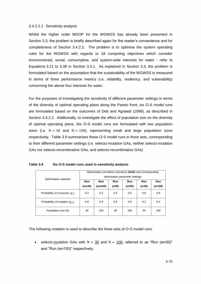
3-75
3.4.2.2.1 Sensitivity analysis
Whilst the higher order MOOP for the WGWSS has already been presented in
Section 3.3, the problem is briefly described again for the reader’s convenience and for
completeness of Section 3.4.2.2. The problem is to optimise the system operating
rules for the WGWSS with regards to 18 competing objectives which consider
environmental, social, consumptive, and system-wide interests for water - refer to
Equations 3.21 to 3.38 in Section 3.3.1. As explained in Section 3.3, the problem is
formulated based on the assumption that the sustainability of the WGWSS is measured
in terms of three performance metrics (i.e. reliability, resiliency, and vulnerability)
concerning the above four interests for water.
For the purposes of investigating the sensitivity of different parameter settings in terms
of the diversity of optimal operating plans along the Pareto front, six O-S model runs
are formulated based on the outcomes of Deb and Agrawal (1999), as described in
Section 3.4.2.2. Additionally, to investigate the effect of population size on the diversity
of optimal operating plans, the O-S model runs are formulated with two population
sizes (i.e. and ), representing small and large population sizes
respectively. Table 3.9 summarises these O-S model runs in three sets, corresponding
to their different parameter settings (i.e. selecto-mutation GAs, neither selecto-mutation
GAs nor selecto-recombinative GAs, and selecto-recombinative GAs)
Table 3.9 Six O-S model runs used in sensitivity analysis
Optimisation operator
Optimisation-simulation scenarios (bold) and corresponding
optimisation parameter settings
Run
(sm30)
Run
(sm100)
Run
(n30)
Run
(n100)
Run
(sr30)
Run
(sr100)
Probability of crossover ( ) 0.2 0.2 0.5 0.5 0.8 0.8
Probability of mutation ( ) 0.8 0.8 0.5 0.5 0.2 0.2
Population size ( ) 30 100 30 100 30 100
The following notation is used to describe the three sets of O-S model runs:
selecto-mutation GAs with 30 and 100, referred to as “Run (sm30)”
and “Run (sm100)” respectively;

3-76
neither selecto-mutation GAs nor selecto-recombinative GAs with 30 and
100, referred to as “Run (n30)” and “Run (n100)” respectively; and
selecto-recombinative GAs with 30 and 100, referred to as “Run
(sr30)” and “Run (sr100)” respectively.
The diversity of the optimal operating plans found by the O-S model in each case is
measured in terms of the crowding distance ( ) as calculated by the NSGA-II (refer
Section 3.4.2). For the purposes of this sensitivity analysis, the optimal operating plans
at the fifth generation are selected for analysis for reasons of the slow convergence to
the Pareto front as described in Section 3.1. Table 3.10 summarises the modelling
results for the six O-S modelling runs in terms of the mean of the crowding distances
( ) for the optimal operating plans.
Table 3.10 Mean crowding distance ( ) of the optimal operating plans for a range of
and values assuming population sizes and
‘ ’ refers to the crowding distance of an operating plan with respect to all 18 objective functions as described in Section 3.4.2 ‘ ’ refers to the probability of crossover as described in Section 3.4.2.1.2
‘ ’ refers to the probability of mutation as described in Section 3.4.2.1.3
The following is a summary of the observations made from the O-S modelling results
presented in Table 3.10 in terms of the overall mean crowding distances (i.e. over the 5
generations):
Runs that used a population size of 30 found operating plans that were
more diverse than those runs that used a population size of 100. This
result is to be expected as the distance between operating plans in the smaller
population would need to be larger in order to cover the same area along the
Generation (t)
Run (sm30) Run (sm100) Run (n30) Run (n100) Run (sr30) Run (sr100)
N = 30 N = 100 N = 30 N = 100 N = 30 N = 100
1 3.095 1.148 3.764 1.305 4.832 1.293
2 3.834 1.188 3.582 1.054 3.954 1.311
3 3.450 1.134 3.999 1.148 4.600 1.329
4 3.651 1.096 4.872 1.249 4.592 1.046
5 3.642 1.175 5.027 1.223 4.272 1.210
Mean 3.534 1.148 4.249 1.196 4.450 1.238
Pm = 0.8 Pm = 0.5 Pm = 0.2
Mean of crowding distances (d) for optimal operating plans
Pc = 0.2 Pc = 0.5 Pc = 0.8

3-77
Pareto front, assuming that the same area is achieved under both population
sizes.
The selecto-recombinative GAs found the most diverse operating plans,
irrespective of the population size.
Therefore, based on these O-S modelling results the following selecto-recombinative
parameter settings are used throughout this thesis:
3.5 Sustainability Indices for the Wimmera-Glenelg Water Supply System
In their study of sustainability criteria for water resource systems, Loucks and Gladwell
(1999) devised an index which could be used to compare the sustainability of one
water management policy to another. Their index measured the performance of water
resource systems over time with respect to the relevant criteria for that system. For the
purposes of this thesis, the index would need to represent a range of stakeholders’
whose varied interests collectively underpin the sustainability of the WGWSS. In a
sense the index would need to be conducive to the preservation of the shared vision for
the operation of the water resource system. Such an index is referred to in this thesis
as a sustainability index.
Belton and Stewart (2002) refer to the following often quoted statement with respect to
the structuring of multi-criteria decision making problems:
“A problem well structured is a problem half solved”
As explained in Section 3.3, the higher order MOOP was structured with the
sustainability of the WGWSS as an overall goal and so it makes for a logical basis on
which to develop a sustainability index. For the reader’s convenience, the value tree
that was used to structure the higher order MOOP for the WGWSS is shown again in
Figure 3.17. Note that this is the same value tree shown in Figure 3.4. For ease of
presentation, the top of the tree is shown to the left of the figure and corresponds to the
highest level criteria, being the sustainability of the WGWSS. The next criteria level

3-78
down represents the four interests for water identified (i.e. environmental, social,
consumptive, and system-wide interests). The third criteria level from the top
represents a further breakdown from the four interests for water of the second level,
and the lowest level criteria represent the 18 conflicting objective functions, to
(refer to Equations 3.21 to 3.38).
Note: ‘ ’ refers to the mth objective function which is defined in Section 3.3.1
Figure 3.17 Value tree of the higher order MOOP for the WGWSS
3.5.1 The Sustainability Index
Figure 3.18 shows the Sustainability Index (referred to here as “the ”) which has
been developed using the value tree of the higher order MOOP for the WGWSS
(Figure 3.17). From top to bottom, there are four levels that constitute the which are
referred to in this thesis as the index, component, indicator, and sub-indicator levels.
Minimum water level at Lake Lonsdale (f5 - Eq 3.25)
Minimum water level at Lake Fyans (f8 - Eq 3.28)
Minimum water level at Rocklands Reservoir (f11 - Eq 3.31)
Environmental flow deficits at 6 locations (f2 - Eq 3.22)
Total water allocation (f17 - Eq 3.37)
Minimum storage levels for recreation amenity
Minimum storage levels for maintenance of water quality
Consumptive user deficits of 30 user groups (f14 - Eq 3.34)
Social interests to water
(Section 3.2.3.2)
Sust
ain
abili
ty o
f WG
WSS
Environmental interests to water
(Section 3.2.3.1)
Environmental flow deficits at 6 locations (f3 - Eq 3.23)
Environmental flow deficits at 6 locations (f1 - Eq 3.21)
Total water allocation (f18 - Eq 3.38)
Total water allocation (f16 - Eq 3.36)
Consumptive user deficits of 30 user groups (f15 - Eq 3.35)
Consumptive user deficits of 30 user groups (f13 - Eq 3.33)
Minimum water level at Rocklands Reservoir (f12 - Eq 3.32)
Minimum water level at Rocklands Reservoir (f10 - Eq 3.30)
Minimum water level at Lake Lonsdale (f4 - Eq 3.24)
Minimum water level at Lake Lonsdale (f6 - Eq 3.26)
Minimum water level at Lake Fyans (f7 - Eq 3.27)
Minimum water level at Lake Fyans (f9 - Eq 3.29)
Environmental flow deficits at 6 locations
Consumptive interests to water
(Section 3.2.3.3)
Consumptive user deficits of 30 user groups
System-wide interests to water
(Section 3.2.3.4)
Total water allocation

3-79
As the index represents an aggregation of the three lower levels, it makes sense to
describe the four levels of the starting at the lowest level and aggregating upwards
towards the itself.
Figure 3.18 The Sustainability Index ( ) for the WGWSS
The lowest level of the is referred to as the sub-indicator level which consists of the
18 performance metrics presented in Section 3.2.4 (refer to Equations 3.3 to 3.20). For
the reader’s convenience and for completeness of the remaining sections under
Section 3.5, these performance metrics are summarised in Equations 3.67 to 3.84.
Note that Equations 3.67 to 3.84 are the same as Equations 3.3 to 3.20. The higher
order MOOP is formulated based on the assumption that the sustainability of the
WGWSS is measured in terms of three performance metrics (i.e. reliability ( ),
resiliency ( ), and vulnerability ( )) for the ith interest for water. Equations 3.67 to
3.69 relate to three environmental ( ) interests for water expressed in terms of nil
environmental flow deficits. Equations 3.70 to 3.78 relate to nine social ( )
Minimum water level at Lake Lonsdale ( ResLL - Eq 3.71)
Minimum water level at Lake Fyans (ResLF - Eq 3.74)
Minimum water level at Rocklands Reservoir (ResRR - Eq 3.77)
Environmental flow deficits at 6 locations (Resenv - Eq 3.68)
Total water allocation (Resalloc - Eq 3.83)
Minimum storage levels for recreation amenity(IIsocio,rec - Eq 3.87)
Minimum storage levels for maintenance of water quality
(IIsocio,wq - Eq 3.88)
Consumptive user deficits of 30 user groups (Rescons - Eq3.80)
Social interests to water
(CIsocio - Eq 3.92)
Sust
ain
abili
ty In
de
x o
f WG
WSS
(SI-
Eq3.
95)
Environmental interests to water
(CIenv - Eq 3.91)
Environmental flow deficits at 6 locations (Vulenv - Eq 3.69)
Environmental flow deficits at 6 locations (Relenv - Eq 3.67)
Total water allocation (Vulalloc - Eq 3.84)
Total water allocation (Relalloc - Eq 3.82)
Consumptive user deficits of 30 user groups (Vulcons – Eq3.81)
Consumptive user deficits of 30 user groups (Relcons - Eq 3.79)
Minimum water level at Rocklands Reservoir (VulRR - Eq 3.78)
Minimum water level at Rocklands Reservoir (RelRR - Eq 3.76)
Minimum water level at Lake Lonsdale (RelLL - Eq 3.70)
Minimum water level at Lake Lonsdale (VulLL - Eq 3.72)
Minimum water level at Lake Fyans (RelLF - Eq 3.73)
Minimum water level at Lake Fyans (VulLF - Eq 3.75)
Environmental flow deficits at 6 locations
(IIenv - Eq 3.86)
Consumptive interests to water
(CIcons - Eq 3.93)
Consumptive user deficits of 30 user groups(IIcons - Eq 3.89)
System-wide interests to water
(CIsys - Eq 3.94)
Total water allocation(IIsys - Eq 3.90)
Sub-indicatorIndicatorComponentIndex

3-80
interests for water expressed in terms of the volume of the storage ( ) being Lake
Lonsdale ( ), Lake Fyans ( ), and Rocklands Reservoir ( ). Equations 3.79 to
3.81 relate to three consumptive ( ) interests for water expressed in terms of nil
supply deficits. Equations 3.82 to 3.84 relate to three system-wide interests for water
expressed in terms of water allocations ( ). These sub-indicators are particularly
important in terms of providing the link between the interests for water in the WGWSS
and the search for candidate optimal operating plans. Thus, the search for candidate
optimal operating plans is relevant to the problem at hand; a desire to develop optimal
operating plans for the WGWSS that have sustainability as an overall goal.
(3.67)
(3.68)
(3.69)
, (3.70)
(3.71)
(3.72)
, (3.73)
(3.74)
(3.75)
, (3.76)
(3.77)
(3.78)
, (3.79)
(3.80)
(3.81)
, (3.82)
(3.83)
(3.84)
Where, ;

3-81
The next level up from the lowest is referred to as the indicator level which represents
an aggregation of the sub-indicators given in Equations 3.67 to 3.84. Before these
indicators are presented it is necessary to present the multiplicative aggregation
scheme which has been adopted for this thesis. This aggregation scheme is based on
the sustainability index developed by Sandoval-Solis et al. (2011) which is
expressed as the geometric average of performance metrics for the th water user as
given by Equation 3.85. Note that the reasons for adopting this aggregation scheme
are explained later this section.
(3.85)
Where,
(note: 0 is the lowest and 1 is the highest level of sustainability
for the th water user)
refers to performance metric, to
refers to the th performance metric for the th water user
Thus, the Indicator-level Index for the ith interest for water ( ) are as follows:
(3.86)
(3.87)
(3.88)
(3.89)
(3.90)
The next level up from the second-lowest is referred to as the component level which
represents a multiplicative aggregation of the indicators given in Equations 3.86 to
3.90. Thus, the Component-level Index for the ith interest for water ( ) are as follows:
(3.91)
(3.92)
(3.93)

3-82
(3.94)
Finally, the sustainability of the WGWSS ( ) represents a multiplicative aggregation of
the components given in Equations 3.91 to 3.94 as follows:
(3.95)
The motivation for using a multiplicative aggregation scheme for the originates from
studies by Loucks (1997), Loucks and Gladwell (1999), and Sandoval-Solis et al.
(2011) in which a sustainability index was proposed for water resources planning and
management. The authors of these studies used performance metrics to evaluate
water management policies and to enable the comparison of alternative policies. One
of the key attractions to their sustainability index was that it could be used to
summarise the performance of alternative policies from the perspective of different
water users. In the context of this thesis, this attribute of the sustainability index is
particularly beneficial as it can be used to explicitly account for all the major interests
for water in the higher order MOOP for the WGWSS.
Note that whilst Equations 3.86 to 3.95 use the same multiplicative aggregation
scheme as that used in Equation 3.85, the for this thesis refers to the sustainability
of the WGWSS in terms of all interests for water collectively as distinct from the single
water user referred to in the (i.e. Equation 3.85). In which case, the may be
thought of as an extension of the aforementioned studies as applied to higher order
MOOPs that concern a range of interests for water. Moreover, Section 3.5.2 goes
further to demonstrate the use of a weighted as part of a process of selecting a
preferred optimal operating plan from the Pareto front.
The following are the main benefits of developing the based on the work by Loucks
(1997), Loucks and Gladwell (1999), and Sandoval-Solis et al. (2011):
Given that the performance metrics must have a value of between 0 and 1
means that the has the flexibility to include a wide range of interests for
water whose competing needs may not necessarily be commensurate.
Moreover, the various interests for water may elect to express their in terms
of any number of performance metrics. For instance, the social interests for
3-83
water in the WGWSS have 9 performance metrics (i.e. Equations 3.68 to 3.76)
compared to the 3 performance metrics for each of the other interests for water.
The three performance metrics as described in Section 3.2.4 (i.e. reliability,
resiliency, and vulnerability) summarise essential performance parameters in a
meaningful manner rather than simply adding broad disparate factors. This is
confirmed by the use of the in the scientific community as cited by Sandoval-
Solis et al. (2011). Moreover, McMahon et al. (2006) goes further to state that
the is the only quantitive measure of sustainability for water resources
systems as it combines the three performance metrics into one index.
The proposed by Sandoval-Solis et al. (2011) uses the geometric average of
the three performance metrics providing better scaling characteristics than the
arithmetic average. For instance, a water user whose reliability, resiliency, and
vulnerability is for each performance metric has an arithmethic average of
and a geometric average of . However,
a water user whose reliability is , resiliency is , and vulnerability is has
an arithmethic average of and a geometric average of . Thus, the scaling
of the does not obscure poor performance as does the arithmethic average.
In the context of this thesis, such scaling characteristics would assist the DM in
reaching consensus amongst competing interests for water by favouring optimal
operating plans that have good values for all metrics. It is worth highlighting
that in cases where the DM has a particular interest in individual metrics (as
opposed to all metrics in the ), the geometric average may tend to penalise
optimal operating plans that have considerable variability in that metric of
interest.
3.5.2 The Weighted Sustainability Index
The process of selecting a preferred optimal operating plan from the Pareto front brings
together two aspects of multi-objective optimisation, namely; (i) the quantitative
information regarding the characteristics of the optimal operating plans along the
Pareto front; and (ii) the higher level qualitative information in the form of stakeholders’
preferences. With reference to the literature on multi-objective optimisation, the
quantitative information relating to the optimal operating plans is analysed in terms of
the objective space and the decision space. As explained in Section 3.5.1, this thesis

3-84
proposes that the be used as the means to evaluate and compare optimal operating
plans in both the objective space and the decision space. With respect to the higher
level qualitative information, it is necessary to develop a conceptual model which
represents stakeholders’ preferences and value judgements. Methods available under
the umbrella term multi-criteria decision analysis (MCDA) are widely used for the
purpose of facilitating the exploration of decisions that take explicit account of multiple
factors or criteria (Belton and Stewart, 2002). As explained in Section 2.3.3, there are
three broad classes of preference models adopted in multi-criteria decision problems
as follows:
Value measurement models associate a real number with each solution (or in
this case optimal operating plan) in order to produce a preference order on the
solutions consistent with the D ’s value judgements.
Goal, aspiration or reference level models set out to establish desirable or
satisfactory levels of achievement for each criterion and then to find optimal
operating plans which are in some sense closest to achieving these desirable
goals or aspirations.
Outranking models undertake a pair-wise comparison of optimal operating
plans to determine the extent to which a preference for one optimal operating
plan compares to another plan. These models set out to establish the strength
of evidence favouring the preference of one optimal plan over another.
The use of the (in evaluating and comparing optimal operating plans) lends itself to
the value measurement preference model. This is due to the providing (i) a means
of associating a real number for each optimal operating plan; and (ii) an ordering or
ranking of these plans, where values of 0 and 1 represent the lowest and highest
levels of sustainability in the WGWSS respectively.
Belton and Stewart (2002) explain that the aforementioned preference models contain
two primary components, namely:
a set of weights which define the relative importance or desirability of achieving
different levels of performance for each criterion; and
an aggregation scheme which allows inter-criteria comparisons or trade-offs in
order to combine preferences across criteria.

3-85
The presented in Section 3.5.1 provides the basis for these two primary components
by allowing for the inclusion of (i) the th stakeholder’s weight for the th performance
metric (
); and (ii) a weighted (geometric average) multiplicative aggregation scheme.
Thus, the Weighted Sustainability Index ( ) for the th stakeholder is expressed as
follows:
(3.96)
Where,
(note: 0 is the lowest and 1 is the highest level of sustainability
for the th stakeholder)
refers to performance metric, to
refers to the th takeholder’ th performance metric
refers to the th takeholder’ weight for the th performance metric
The has all the benefits of the in terms of flexibility and scalability as mentioned
in Section 3.5.1 and provides continuity in the multi-criterial decision-making process
i.e. from evaluation and comparison of optimal operating plans through to the selection
of a preferred optimal operating plan. Figure 3.19 summarises the th stakeholder’s
Weighted Component-level Index for the ith interest for water ( ) and the Weighted
Sustainability Index ( ) for the WGWSS.
It is important to highlight the following reasons for using the th stakeholder’s weights
at the sub-indicator level for the and the :
the weights at the sub-indicator level represent the least amount of subjectivity
(compared to all other levels of the ) given that these are not aggregates of
lower levels of the . This means that the selection of a preferred optimal
operating plan is affected by the least amount of bias that may exist amongst
stakeholders compared to other levels of the ; and

3-86
subjectivity (through the use of weights) is introduced a posteriori (post-
optimisation) and so weights may be revised without having to necessarily
repeat the optimisation process. This may lead to a reduction in the
computational effort involved in the search for and selection of optimal
operating plans during the process of stakeholder negotiations.
Figure 3.19 The th
stakeholder’s Weighted Sustainability Index ( ) for the WGWSS
Modifying Equations 3.91 to 3.95 in line with Equation 3.96 gives the th stakeholder’s
Weighted Component-level Index for the ith interest for water ( ) and the Weighted
Sustainability Index ( ) for the WGWSS as follows:
Minimum water level at Lake Lonsdale (Res jLL
w jLL)
Minimum water level at Lake Fyans (Res jLF
w jLF)
Minimum water level at Rocklands Reservoir (Res jRR
w jRR)
Environmental flow deficits at 6 locations (Res jenv
w jenv)
Total water allocation (Res jalloc
w jalloc)
Minimum storage levels for recreation amenity
Minimum storage levels for maintenance of water quality
Sub-indicatorIndicatorComponent
Consumptive user deficits of 30 user groups (Res jcons
w jcons)
Index
Social interests to water
(CI jsocio - Eq 3.98)
We
igh
ted
Su
stai
nab
ility
Ind
ex
of W
GW
SS (S
Ij-E
q3.
101)
Environmental interests to water
(CI jenv - Eq 3.97)
Environmental flow deficits at 6 locations (Vuljenv
w jenv)
Environmental flow deficits at 6 locations (Reljenv
w jenv)
Total water allocation (Vuljalloc
w jalloc)
Total water allocation (Reljalloc
w jalloc)
Consumptive user deficits of 30 user groups (Vuljcons
w jcons)
Consumptive user deficits of 30 user groups (Reljcons
w jcons)
Minimum water level at Rocklands Reservoir (VuljRR
w jRR)
Minimum water level at Rocklands Reservoir (ReljRR
w jRR)
Minimum water level at Lake Lonsdale (ReljLL
w jLL)
Minimum water level at Lake Lonsdale (VuljLL
w jLL)
Minimum water level at Lake Fyans (ReljLF
w jLF)
Minimum water level at Lake Fyans (VuljLF
w jLF)
Environmental flow deficits at 6 locations
Consumptive interests to water
(CI jcons - Eq 3.99)
Consumptive user deficits of 30 user groups
System-wide interests to water
(CI jsys - Eq 3.100)
Total water allocation
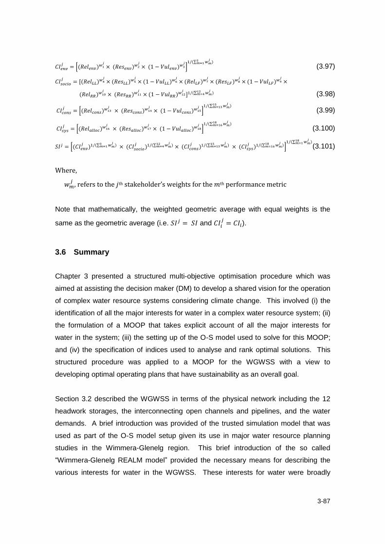
3-87
(3.97)
(3.98)
(3.99)
(3.100)
(3.101)
Where,
, refers to the th takeholder’ weight for the th performance metric
Note that mathematically, the weighted geometric average with equal weights is the
same as the geometric average (i.e. and ).
3.6 Summary
Chapter 3 presented a structured multi-objective optimisation procedure which was
aimed at assisting the decision maker (DM) to develop a shared vision for the operation
of complex water resource systems considering climate change. This involved (i) the
identification of all the major interests for water in a complex water resource system; (ii)
the formulation of a MOOP that takes explicit account of all the major interests for
water in the system; (iii) the setting up of the O-S model used to solve for this MOOP;
and (iv) the specification of indices used to analyse and rank optimal solutions. This
structured procedure was applied to a MOOP for the WGWSS with a view to
developing optimal operating plans that have sustainability as an overall goal.
Section 3.2 described the WGWSS in terms of the physical network including the 12
headwork storages, the interconnecting open channels and pipelines, and the water
demands. A brief introduction was provided of the trusted simulation model that was
used as part of the O-S model setup given its use in major water resource planning
studies in the Wimmera-Glenelg region. This brief introduction of the so called
“Wimmera-Glenelg REALM model” provided the necessary means for describing the
various interests for water in the WGWSS. These interests for water were broadly
3-88
categorised into those which represented environmental ( ); social ( ) i.e.
recreation at Lake Lonsdale ( ) and at Lake Fyans ( ), and for water quality at
Rocklands Reservoir ( ); consumptive ( ); and those that affected all users
system-wide in terms of water allocations ( ). In each case, the process of
identifying the four interests for water involved developing an understanding of the
model configuration for that particular user together with any relevant criteria by which
to evaluate candidate optimal operating plans. For instance in the case of the
environmental interests for water, flow requirements were configured in the Wimmera-
Glenelg REALM model as separate EWDs in order to provide for the required flows in
the various stream reaches. In which case, the criterion that was used to evaluate
candidate optimal operating plans with respect to EWDs was the difference between
the amount that was required at a particular location (i.e. demand) and the amount that
was provided to that location (i.e. supply). Such criteria together with three broad
performance metrics for the th interest for water, being reliability ( ), resiliency
( ), and vulnerability ( ), served as the basis for the objective functions used in
the formulation of the MOOP. A total of 18 performance metrics were used to evaluate
candidate optimal operating plans on a quantitative basis with respect to the four
interests for water identified viz. environmental (i.e. , , and ), social
(i.e. , , , , , , , , and ), consumptive
(i.e. , , and ), and the system-wide interests (i.e. ,
, and ).
Section 3.3 presented the formulation of the higher order MOOP in terms of a
hierarchical structure for which the sustainability of the WGWSS was assumed to
represent the highest level criteria. The second level of the problem hierarchy
represented the four major interests for water (i.e. environmental, social, consumptive,
and system-wide interests) and the lowest level criteria represented the 18 objective
functions for the MOOP. Structuring the higher order MOOP in this way provided the
necessary means for (i) taking explicit account of all the major interests for water in the
WGWSS; and (ii) the evaluation of candidate optimal operating plans. It was also
explained that formulating a higher order MOOP using higher criteria levels (e.g. the
four interests for water) would have the effect of reducing the dimensionality of the
problem whereas lower criteria levels (e.g. the 18 objective functions) would have the
reverse effect. It was explained that the objective functions of a MOOP play a role of
guiding the optimisation search towards candidate optimal operating plans that perform

3-89
the best in terms of the values of these objective functions. The 18 objective functions
of the higher order MOOP were formulated using the aforementioned 18 performance
metrics. Thus, the sustainability of the WGWSS was measured in terms of maximising
the reliability ( ), maximising the resiliency ( ), and minimising the vulnerability
( ) of the th interest for water. The decision variables for the higher order MOOP
were expressed in terms of 24 water management planning decisions representing the
key operating rules which control and regulate the water resources within the WGWSS.
The mathematical equations for the 24 decision variables were presented in terms of
the six areas of system operation viz. (i) priorities of supply (i.e. to ); (ii) a
storage flood reserve volume (i.e. ); (iii) environmental allocation shares (i.e. to
); (iv) flow paths (i.e. and ); (v) storage maximum operating volumes (i.e.
to ); and (vi) storage draw down priorities and storage targets (i.e. to
). These planning decisions were collectively referred to as an “operating plan.”
The constraints of the problem were specified both in terms of the formulation of the
MOOP (i.e. as bounds on variables and as integer constraints) and also in terms of the
real-world limitations of the WGWSS (i.e. as statutory constraints and as physical
constraints). By far, most of the problem constraints were already configured in the
Wimmera-Glenelg REALM model. It was explained that this was one of the major
benefits of using an O-S modelling approach in that many of the complexities of a real-
world water resource system were already configured in existing well trusted simulation
models.
Section 3.4 described the setup of the O-S model that was used to solve the higher
order MOOP in Section 3.3. An overview of the O-S modelling procedure was provided
starting from the initial population of randomly generated operating plans through to the
final population of optimal operating plans. As the initial population required the
execution of the Wimmera-Glenelg REALM model, the setup of the simulation engine
was presented in the first instance, in terms of the system file and data inputs. It was
explained that the original simulation model, known as the WMPP2104.sys file, was
replaced by a surrogate model in order to (i) improve its flexibility and stability in terms
of changing from one set of operating rules to another; and (ii) exchange information
between it and the optimisation engine so that the O-S model could successfully iterate
to the population of optimal operating plans. This lower-fidelity physically based
surrogate model was referred to as the “Wimmera-Glenelg REALM model” and showed
a good fit with the WMPP2104.sys file (i.e. Nash-Sutcliffe efficiency index, ).

3-90
The most significant difference between the WMPP2104.sys file and the Wimmera-
Glenelg REALM model was that the latter model had revised many of the carrier
penalties which were interfering with the storage targets. This change resulted in a
marked improvement in the stability of the Wimmera-Glenelg REALM model in terms of
a reduced number of convergence failures. A brief summary was provided in terms of
the methodology for the derivation of the hydro-climatic and water demand inputs for
the three hydro-climatic conditions viz. historic, low to medium level, and medium to
high level GHG emissions. It was explained that there were 9 rainfall inputs, 18
evaporation inputs, and 21 streamflow inputs which represented one of the three
hydro-climatic conditions; 30 consumptive water demands which were static and the
same for all three hydro-climatic conditions; and 6 environment water demands
(EWDs) which had a static and a variable component. The setup of the optimisation
engine was described in terms of the detailed workings of the NSGA-II. The sorting
procedure of the NSGA-II was presented in the first instance together with the niching
strategy (which uses the crowding distance ( )). It was explained that the niching
strategy provided a means for ensuring a diverse set of operating plans with the
continued convergence of the NSGA-II towards the Pareto front. The genetic operators
(i.e. selection, crossover, and mutation) were described in terms of a sample higher
order MOOP starting from the parent population through to the offspring population of
candidate optimal operating plans. The adoption of the optimisation parameters largely
relied on the outcomes of separate studies together with six O-S model runs which
were used to show the sensitivity of different optimisation parameter settings in terms
of the diversity of optimal operating plans along the Pareto front. The adopted
optimisation parameters were .
Section 3.5 presented sustainability indices for the WGWSS which were developed for
the purposes of analysing and ranking optimal operating plans from the Pareto front.
The Sustainability Index ( ) for the WGWSS was developed from the hierarchical
structure of the higher order MOOP described in Section 3.3. The highest level
represented the which was used to evaluate optimal operating plans with respect to
all the major interests for water in the WGWSS. The second level of the was
expressed in terms of a Component-level Index for the ith interest for water ( ) viz.
( ) for the environmental interests, ( ) for the social interests, ( ) for the
consumptive interests and ( ) for the system-wide interests for water. The lowest
level of the featured the 18 performance metrics which were used to provide the

3-91
important link between the interests for water in the WGWSS and the search for
candidate optimal operating plans. As such, it was shown that the provided the
basis for the development of optimal operating plans for the WGWSS which have
sustainability as an overall goal. The reasons for using a multiplicative aggregation
scheme for the were explained. The main benefits of this geometric average
aggregation were that the would have increased flexibility to include a wide range of
interests for water and to express these in terms of any number of performance
metrics; and that it would have better scaling characteristics so that the would not
obscure poor performance as compared to the arithmethic average. It was considered
that such scaling characteristics would assist the DM to reach consensus amongst
competing interests for water by favouring optimal operating plans that had good
values for all metrics (of all interests for water). It was explained that the process of
ranking optimal operating plans from the Pareto front brought together two aspects of
multi-objective optimisation, namely; (i) the quantitative information regarding the
characteristics of the optimal operating plans along the Pareto front; and (ii) the higher
level qualitative information in the form of stakeholders’ preferences. The quantitative
information was provided by the and its ability to evaluate and compare optimal
operating plans in both the objective space and the decision space. With respect to the
qualitative information, the use of the was extended to incorporate (i) the th
stakeholder’s weight for the th performance metric (
); and (ii) a weighted
(geometric average) multiplicative aggregation scheme. The resulting weighted
sustainability index was referred to as the “Weighted Sustainability Index” ( ) for the
th stakeholder. It was explained that the had all the benefits of the in terms of
flexibility and scalability as described earlier and that it also provided continuity in the
multi-criterial decision-making process i.e. from evaluation of optimal operating plans
through to the selection of a preferred optimal operating plan.

4-1
Chapter 4. Analysis of optimal operating plans using the Sustainability Index ( )
4.1 Introduction
This chapter describes the effectiveness of the Sustainability Index ( ) in terms of
analysing optimal operating plans along the Pareto front obtained using multi-objective
optimisation under historical hydro-climatic conditions. Specifically, it presents an
analytical approach that deals with (i) ranking alternatives; (ii) assessing the level of
influence that a set of operating rules has on a system’s sustainability; and (iii) showing
the effect of alternative operating plans on various interests for water. For this
purpose, various multi-objective optimisation problems (MOOPs) are formulated for the
Wimmera-Glenelg Water Supply System (refer Figure 4.1) and solved using the
optimisation-simulation (O-S) modelling approach described in Chapter 3. Note that
Figure 4.1 is the same schematic previously used in Figure 3.2.
Note: Numbers in brackets refer to environmental water demands or EWDs (italic font) and consumptive water demands (regular font) configured in the Wimmera-Glenelg REALM model (refer to Section 3.2.2).
Figure 4.1 Schematic of the Wimmera-Glenelg Water Supply System (not to scale)
Pipeline
EWD
Diversion structure
to Terminal lakes
to Avon-Richardson rivers
Open channel
Consumptive user
(11) to (18)
Lake Fyans
Lake Lonsdale
Waterway
Lake Bellfield
HorshamLake Wartook
Rocklands Reservoir
Moora MooraReservoir
(6) to (9)
Toolondo Reservoir
Pine Lake
Taylors Lake
(2) to (5)
(10)
(1)
(19) to (30)
Fyan
s Creek
Wimmera
River
Burnt C
reek
Dock& Green lakes
(2)
(6)
(5)
(1)
(4)
(3)
from Wannon River
Wimmera Mallee Pipeline (WMP)
N

4-2
Chapter 3 described important factors related to solving higher order MOOPs which
influenced the research methodology, viz; the slow convergence of solutions to the
Pareto front; and the high computational costs required to progress this search. An
increase in objectives has the effect of slowing the progression (i.e. convergence) of
the population of solutions to the Pareto front. This slow convergence is largely
attributed to the dominance test which is applied to the solutions of the population;
resulting in a greater number of O-S modelling generations to progress the solutions
towards the Pareto front. The term generation refers to a (single) iteration of the O-S
model. An increase in the number of generations requires greater computational
processing effort, which may be addressed through parallel computing processes.
However, such parallel computing capabilities were not available for this thesis, which
meant that simulation runs for all solutions of the population had to be completed in
series (i.e. one run at a time) before the optimisation search could be executed. For
these reasons (of slow convergence and high computational costs), the number of
generations performed by the O-S model was limited to five in number (throughout this
thesis). Importantly, this is not to be mistaken as a research limitation given that the
novelty of this study is that of the structured multi-objective optimisation procedure
rather than finding Pareto fronts per se.
Chapter 3 also described an approach for the formulation of MOOPs and applied it to a
higher order MOOP which was used to support the development of optimal operating
plans for the Wimmera-Glenelg Water Supply System (WGWSS). A higher order
MOOP is defined in this thesis as a problem that is formulated with more than three
objective functions. All the major interests for water were explicitly taken into account
and were used as the basis for 18 objective functions which directed the search
towards the set of optimal operating plans which were collectively referred to as the
Pareto front. The decision variables were expressed in terms of 24 water management
planning decisions representing the key operating rules which control and regulate the
water resources within the WGWSS. For the reader’s convenience and for
completeness of Chapter 4, these planning decisions are provided again in Table 4.1.
There are six categories of decision variables representing priorities of supply between
different sources of supply and between different user groups; storage flood reserve
volumes to provide flood attenuation; environmental allocation shares for apportioning
environmental water allocations between river basins; the preference of alternative flow
paths for the harvesting and/or transfer of water; storage maximum operating volumes

4-3
for the key water harvesting storages; and storage draw down priorities and storage
targets.
Table 4.1 Water management planning decisions for the WGWSS
Category Decisions Value range
Priority of supply
Should Moora Moora Reservoir be the first priority of
supply or Lake Wartook to demands (2) to (5) and EWDs in MacKenzie River (3) and Burnt Creek (4)?
Either Lake Wartook or Moora Moora Reservoir is first priority and the other is a
supplementary source of supply
Should Horsham (1) be supplied in preference to the EWD
in MacKenzie River at Dad and Dave Weir (2) or vice versa?
Either Horsham (1) or EWD (2) is satisfied first
Should water be harvested into Taylors Lake in preference to meeting the EWD in MacKenzie River (3) or vice versa?
Either harvest flows into Taylors Lake or EWD (3) is satisfied first
Should water be harvested into Taylors Lake in preference
to meeting the EWD in Burnt Creek (4) or vice versa? Either harvest flows into Taylors Lake or
EWD (4) is satisfied first
Should consumptive demands (6) to (9) be satisfied before
the EWDs in Glenelg River (1) or vice versa? Either consumptive demands (6) to (9) or
EWD (1) is satisfied first
Should water be harvested into Wimmera Inlet Channel
(WIC) in preference to meeting passing flows in Wimmera River at Huddlestons Weir or vice versa?
Either harvest flows into WIC or provide passing flow (6) first
Should water be held in storage for supply to consumptive
demands (19) to (30) in preference to the EWD in Mt William Creek at Lake Lonsdale (5) or vice versa?
Either hold water in Lake Lonsdale for consumptive demands (19) to (30) or supply
EWD (5) first
Flood reserve volume
How much flood reserve should be provided at Lake
Wartook in June? Either hold no reserve or hold a maximum of
up to the full storage capacity in June
Share of environ-mental
allocation
How much of the environmental water allocation should be
released in the Glenelg River basin? Either no share or up to 100% of the
environmental water allocation
How much of the environmental water allocation should be
released in the Wimmera River basin at Lake Wartook?
Either no share or up to the remaining share of the environmental water allocation after that provided for the Glenelg River basin
How much of the environmental water allocation should be released in the Wimmera River basin at Lake Lonsdale?
Either no share or up to the remaining share of the environmental water allocation after
that provided for the Glenelg River basin and that at Lake Wartook
Flow path
Should Mt William Creek flows be harvested into Wimmera Inlet Channel or should all these flows be passed down to
Wimmera River?
Either harvest flows into Wimmera Inlet Channel or pass all flows to Wimmera River
Should water from Lake Bellfield be mixed with water from
Taylors Lake via the Bellfield-Taylors Pipeline?
Supply from Lake Bellfield may result in one of three outcomes; nil, a proportion based on
the volume in storage, or 100%
Storage maximum operating volume
Toolondo Reservoir 0 to 92,430 ML
Lake Lonsdale Inlet is either open or closed
Lake Bellfield 0 to 76,000 ML
Taylors Lake 0 to 33,700 ML
Rocklands Reservoir 0 to 348,000 ML
Lake Lonsdale 0 to 65,000 ML
Moora Moora Reservoir 0 to 6,300 ML
Storage draw down
priority and
storage target
What should be the drawdown priority of the headworks
storages? Each storage is assigned a unique draw
down priority from 1 to 8
What should be the second point on the target curve for
the headworks storages? Any volume between dead storage and FSL
What should be the third point on the target curve for the
headworks storages? Any volume between the second target point
and FSL
What should be the fourth point on the target curve for the
headworks storages? Any volume between the third target point
and FSL
‘ ’ refers to decision variable which are defined in Section 3.3.2. ‘EWDs’ refers to environmental water demands. Number in brackets refers to consumptive user demand centres and environmental flow sites shown in Figure 4.1.

4-4
Chapter 3 presented the as a means to evaluate and compare alternative operating
plans and highlighted the following key benefits to the use of the in higher order
MOOPs:
a) The provides a link between the interests for water and the objective
functions as part of the formulation of the MOOP and so allows for the search
of optimal operating plans that are relevant to the DM. This potentially
increases the efficiency of the search process and reduces computational
effort. The search process here refers to the progression of the O-S modelling
procedure towards the Pareto front.
b) By virtue of the being applied after the optimal operating plans are found by
the O-S modelling approach -
The is consistent with the ideal multi-objective optimisation approach.
Deb (2001) described the ideal multi-objective optimisation approach in two
steps where the first step involves finding a diverse set of optimal solutions
and the second step involves choosing one of the solutions using higher-
level qualitative information. It was shown that the could be used as part
of the second step given its mathematical structure was able to be adapted
for the inclusion of the D s’ relative weights.
The does not introduce bias in the search process. As the O-S
modelling procedure is performed before the , all objectives are
considered to be equally important.
The avoids the need to repeat the search process in situations where the
D ’s preferences change over time. D s’ preferences may change over
time due to the social learning process that occurs as part of the selection
of a preferred optimal solution.
One of the main constituents of the were described in terms of four component-level
indices that are used for the evaluation and comparison of optimal operating plans
within Chapter 4. For the reader’s convenience and for completeness of Chapter 4
these component-level indices are provided again in Equations 4.1 to 4.4. The
Component-level Index ( ) assumes that the sustainability for the ith interest for water
is measured in terms of reliability ( ), resiliency ( ), and vulnerability ( ).

4-5
These interests for water identified in Chapter 3 are broadly classified into
environmental ( ); social interests such as for recreation at Lake Lonsdale ( ), Lake
Fyans ( ), and Rocklands Reservoir ( ); consumptive interests ( ); and all these
interests collectively in terms of system water allocations ( ). Equation 4.5 is the
mathematical expression for the . The reader is referred to Section 3.5.1 for further
details regarding the basis of these equations.
(4.1)
(4.2)
(4.3)
(4.4)
(4.5)
For the purposes of assessing the effectiveness of the in terms of ranking optimal
operating plans, a lower order MOOP concerning environmental flows is presented. A
lower order MOOP is a problem that is formulated with two or three objective functions.
The three environmental objectives are expressed in terms of environmental flow
deficits and are defined in Section 4.2.1. This MOOP is solved for seven decision
variables that represent the storage maximum operating volumes of six headworks
storages within the WGWSS (refer to Table 4.1 - to ). As explained in Section
3.3.1.5, maximum operating volumes are used to provide environmental (unregulated)
flows in the form of storage spills and also to reduce storage evaporative losses. In
general, a system which has very high maximum operating volumes runs the risk of not
delivering the required frequency and volume of large environmental flows (or “high
fresh flows”). Conversely, a system which has very low maximum operating volumes
runs the risk of not being able to reserve sufficient resources for essential services
during periods of low inflow. The O-S modelling results for the optimal operating plans
are analysed in terms of the objective space and the decision space. In the objective
space, the results are presented as a three dimensional Pareto front using a Cartesian
coordinate system. This visualisation approach is compared to an equivalent
representation using the in terms of its normalised rank (referred to as “ curve”).
Similarly, the decision variables for each of the optimal operating plans found are also
presented and analysed with respect to the curve. Refer to Section 4.2 for details of
this part of the study.
4-6
The level of influence that a set of operating rules has on the sustainability of the
WGWSS is assessed using a series of higher order MOOPs. A higher order MOOP is
a problem that is formulated with more than three objective functions. The higher order
OOP described in Chapter 3 (referred to as “Run (A1)”) is also included as a point of
reference. For each O-S modelling run, an 18-objective problem is used to search for
optimal operating plans assuming all but one of the planning decision categories are
fixed, at any one time, to the decision variable values as per the simulation-only base
case scenario (BC01). The base case scenario represents the operating plan that is in
place for the WGWSS at the time of writing of this thesis – refer to Section 3.2.2 for
further details. Solving for one planning decision category in this way focuses the
search on a certain section of the Pareto front and allows the exploration of optimal
plans with respect to one category of operating rules. This approach produces six O-S
modelling runs in total. Building on the outcomes of the lower order MOOP, the optimal
operating plans found under the six runs are presented in terms of curves and
compared to Run (A1) in order to assess the level of influence each category of
operating rules has on the sustainability of the WGWSS. Refer to Section 4.3 for
details of this part of the study.
Having applied the to a lower order MOOP (Section 4.2) and a series of higher order
MOOPs (Section 4.3), this understanding of the can be used to show the effect of
alternative operating plans on various interests for water in terms of their corresponding
(i.e. , , , and ). This part of the study does not introduce any
additional O-S model runs; instead it investigates two optimal operating plans under the
aforementioned Run (A1) in terms of the objective space and decision space. In order
to appreciate the full range of optimal operating plans that have been found, the two
plans selected for analysis correspond to those that achieve the highest and lowest .
As for the , the operating plans are also compared using the in terms of its
normalised rank (referred to as “ curve”). These operating plans are compared to the
base case operating plan (BC01) in order to highlight the differences in system
behaviour over the planning period. Refer to Section 4.4 for details of this part of the
study.

4-7
4.2 A lower order MOOP - one user group
The purpose of the lower order MOOP presented in this section is to assess the
effectiveness of the curve in the visualisation of the optimal operating plans that lie
on the Pareto front. A lower order MOOP is used for this investigation as the modelling
results can be presented on a two dimensional plane whereby each orthogonal axis
represents an objective function. Such a visual representation allows for the
exploration of a three dimensional Pareto front using a Cartesian coordinate system.
This visualisation approach is compared to the corresponding curve.
4.2.1 Problem formulation and model setup
The problem is to optimise the system operating rules with regards to three
environmental objectives expressed in terms of nil environmental flow deficits which
seek to maximise the reliability, maximise the resiliency, and minimise the vulnerability
of such deficits (refer to Section 3.2.4 for further details regarding these performance
metrics). In simple terms, nil environmental flow deficits may be thought of as
environmental flow demands that do not experience any shortfall in supply volume.
The three objectives are given below in Equations 4.6 to 4.8 and are based on
performance metrics as described in Sandoval-Solis et al. (2011). These objectives
are in direct conflict with each other as increasing the reliability of nil environmental
flow deficits does not necessarily equate to an increase in resiliency; nor does the
increase in any or both of these two objectives (i.e. reliability and resiliency) result in
reduced vulnerability of such deficits, and vice versa. For each time period
, the annual environmental flow deficits are positive when
the annual environmental water demand is more than the annual water
supplied , and when the water supplied is equal to the water demand
the annual environmental flow deficits are zero
. For this problem,
represents the annual sum of six
separate environmental flow deficits in the Glenelg River at Rocklands Reservoir,
Wimmera River at Huddlestons Weir, Mt William Creek at Lake Lonsdale, MacKenzie
River at Dad and Dave Weir, MacKenzie River at Distribution Heads, and Burnt Creek
at Burnt Creek Channel (refer Figure 4.1). The number of time intervals
corresponds to the 118-year simulation period from 1891 to 2009.

4-8
(4.6)
(4.7)
(4.8)
Subject to the constraints as configured in the revised Wimmera-Glenelg
REALM model (refer Section 3.3.2).
The decision variables to solve for are to corresponding to those
that define the maximum operating volumes for the storages specified in
Table 4.1.
The lower order MOOP is solved for five generations using the O-S modelling
approach with the following optimisation parameters: population size ,
probability of crossover , and probability of mutation (refer to
Section 3.4.2.2 for further details regarding the optimisation parameters adopted).
It is important to highlight that as this lower order MOOP considers environmental
objectives only, the O-S model may well find optimal operating plans that are not
practical in a real world sense. For example, the O-S model may find an optimal
operating plan that specifies a very low maximum operating volume for a storage that is
the sole source of supply to consumptive users. Whilst the low maximum operating
volume would provide high fresh flows to the waterway downstream of the storage, it
could possibly cause a poor result in terms of consumptive user supply deficits in an
otherwise different MOOP which includes consumptive use objectives.
4.2.2 Modelling results and discussion
4.2.2.1 Objective space
The O-S model found a total of six optimal operating plans after 1,500 simulations and
4,500 objective function evaluations i.e. a population of 100 operating plans over a
period of 5 generations assuming a 3-stage evolutionary process (or 100 x 5 x 3 =
1,500 simulations), each simulation requiring evaluations with respect to 3-objective
functions (or 1,500 x 3 = 4,500 evaluations). The 3-stage evolutionary process used in
the Elitist Non-Dominated Sorting Genetic Algorithm (NSGA-II) is explained in Section

4-9
2.3.1.2(a). The remaining 94 operating plans were either duplicates of the six optimal
plans or inferior with respect to these six plans (refer Equation 2.2 for further details
regarding the possible outcomes from the dominance test). Figure 4.2 shows the six
optimal operating plans and also the base case operating plan (BC01) which is
included as a point of reference.
Figure 4.2 3-D (x-y-z) plot of six optimal operating plans for the lower order MOOP
and the base case operating plan (BC01)
The visualisation of the Pareto front for this lower order MOOP is straightforward using
a three-dimensional Cartesian coordinate plane. For ease of analysis of the Pareto
front, the corresponding two-dimensional plots for ( ) and ( ) , ( )
and ( ) , and ( ) and ( ) are also provided in Figure 4.3,
Figure 4.4, and Figure 4.5 respectively.
00.2
0.40.6
0.81
0
0.2
0.4
0.6
0.8
1
0
0.2
0.4
0.6
0.8
1
Rel(env)
Max Rel(env) vs Max Res(env) vs Min Vul(env)
Res(env)
Vul(env)
Max vs Max vs Min(f1) Relenv (f2) Resenv (f3) Vulenv
(f 1) Relenv (%)
(f 2) Resenv (%)
(f3)
Vu
l en
v (%
)
80
60
40
20
0
100
80
60
40
20
0
100
8060
4020
0
100
Plan no. 1
Plan no. 2
Plan no. 3
Plan no. 4
Plan no. 5
Plan no. 6
BC01
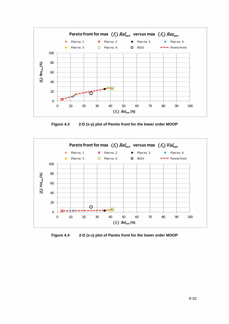
4-10
Figure 4.3 2-D (x-y) plot of Pareto front for the lower order MOOP
Figure 4.4 2-D (x-z) plot of Pareto front for the lower order MOOP
0
20
40
60
80
100
0 10 20 30 40 50 60 70 80 90 100
Pareto front for max Relenv versus max Relcons
Plan no. 1 Plan no. 2 Plan no. 3 Plan no. 4
Plan no. 5 Plan no. 6 BC01 Pareto front
(f1) Relenv
(f 1) Relenv (%)
(f2)
Res
en
v(%
)
(f2) Resenv
0
20
40
60
80
100
0 10 20 30 40 50 60 70 80 90 100
Pareto front for max Relenv versus max Relcons
Plan no. 1 Plan no. 2 Plan no. 3 Plan no. 4
Plan no. 5 Plan no. 6 BC01 Pareto front
(f1) Relenv
(f 1) Relenv (%)
(f3)
Vu
l en
v(%
)
(f3) Vulenv

4-11
Figure 4.5 2-D (y-z) plot of Pareto front for the lower order MOOP
Table 4.2 summarises the change in reliability, resiliency, and vulnerability of operating
Plan no. 1 to Plan no. 6 relative to BC01 based on the results shown in Figure 4.3,
Figure 4.4, and Figure 4.5 respectively. The tabular results below confirm that the
reason that BC01 does not lie on the Pareto front (as shown in Figure 4.3 to Figure 4.5)
is because it is worse than Plan no. 6, Plan no. 5, and Plan no. 3 in all objectives.
Table 4.2 Change in reliability, resiliency, and vulnerability of Plan no. 1 to
Plan no. 6 relative to the base case operating plan (BC01)
The differences shown in Table 4.2 are used as a means to trade-off each of the six
optimal operating plans against BC01. For example, selecting Plan no. 6 in preference
0
20
40
60
80
100
0 10 20 30 40 50 60 70 80 90 100
Pareto front for max Relenv versus max Relcons
Plan no. 1 Plan no. 2 Plan no. 3 Plan no. 4
Plan no. 5 Plan no. 6 BC01 Pareto front
(f2) Resenv
(f 2) Resenv (%)
(f3)
Vu
l en
v(%
)
(f3) Vulenv
(f 1) Rel env (f 2) Res env (f 3) Vul env
Plan no. 1 -11.9% (13.6% - 25.4%) -2.2% (13.7% - 15.9%) -7.5% (2.9% - 10.4%)
Plan no. 2 -22.0% (3.4% - 25.4%) -12.4% (3.5% - 15.9%) -8.2% (2.2% - 10.4%)
Plan no. 3 10.2% (35.6% - 25.4%) 9.1% (25.0% - 15.9%) -7.0% (3.4% - 10.4%)
Plan no. 4 -13.6% (11.9% - 25.4%) -6.3% (9.6% - 15.9%) -7.6% (2.8% - 10.4%)
Plan no. 5 12.7% (38.1% - 25.4%) 11.5% (27.4% - 15.9%) -6.1% (4.4% - 10.4%)
Plan no. 6 16.1% (41.5% - 25.4%) 10.2% (26.1% - 15.9%) -5.2% (5.2% - 10.4%)
BC01 na na na
'na ' means not appl icable
Change in reliability (Rel ), resiliency (Res ), and vulnerability (Vul ) of
Plan no. 1 to Plan no. 6 relative to base case operating plan (BC01)

4-12
to BC01 means that the operating rules would achieve nil environmental flow deficits
that are 16.1% more reliable, 10.2% more resilient and 5.2% less vulnerable than the
deficits under BC01. In this instance, Plan no. 6 is clearly the better solution with
respect to all objectives. Comparing the results for Plan no. 2 with BC01, shows that
the operating rules under Plan no. 2 would achieve nil environmental flow deficits that
are 22% less reliable, 12.4% less resilient, and 8.2% less vulnerable than the deficits
under BC01. Despite BC01 achieving a better result than Plan no. 2 in terms of two
objectives (i.e. reliability and resiliency), Plan no. 2 is not inferior to BC01 as Plan no. 2
is better than BC01 in at least one objective (i.e. vulnerability).
From Equation 4.1, the Component-level Index ( ) values for each of the six
optimal operating plans found and BC01 are calculated and ranked from highest to
lowest in Table 4.3 and plotted against its normalised rank in Figure 4.6. Note that
as this MOOP concerns environmental interests for water only, in the
absence of any other component-level index. Both Table 4.3 and Figure 4.6 show that
the of Plan no. 6 is the highest ( ) and Plan no. 2 is the lowest ( ). Note that
the of BC01 (i.e. ) is not included in Table 4.3 and Figure 4.6 as BC01 does not
lie on the Pareto front.
Table 4.3 Objective function value, Sustainability Index, and crowding distance for
optimal operating plans
Table 4.3 also shows the crowding distance (d) for all six optimal operating plans. As
explained in Section 2.3.1.2(a), the crowding distance is a measure of the density of
solutions surrounding a particular solution in the population with respect to all
objectives. It represents the diversity amongst optimal operating plans along the
Pareto front. Note that the crowding distances for Plan no. 6, Plan no. 5, and Plan no.
2 are equal to ∞ as these are considered to be boundary solutions in the crowding
(f 1) Rel env (f 2) Res env (f 3) Vul env
Plan no. 6 41.5% 26.1% 5.2% 0.47 ∞ na
Plan no. 5 38.1% 27.4% 4.4% 0.46 ∞ na
Plan no. 3 35.6% 25.0% 3.4% 0.44 1.65
Plan no. 4 11.9% 9.6% 2.8% 0.22 0.92
Plan no. 2 3.4% 3.5% 2.2% 0.11 ∞ na
BC01 25.4% 15.9% 10.4% na na na
'na ' means not appl icable
1.451.55
1.18Plan no. 1 13.6% 13.7% 2.9% 0.26
Objective function value Average crowding
distance (dav)
Sustainability
Index (SI )
Crowding
distance (d)

4-13
distance calculation. The average of the crowding distances (dav) for Plan no. 3 and
Plan no. 1 is greater than that for Plan no. 1 and Plan no. 4 i.e. . Note that
the crowding distances for Plan no. 6, Plan no. 5, and Plan no. 2 are not included in the
average crowding distance as these are considered to be boundary solutions as
mentioned earlier. This means that Plan no. 1 and Plan no. 4 are more tightly clumped
together than Plan no. 3 and Plan no. 1. This effect is shown graphically in Figure 4.6
whereby the gradient in the curve between Plan no. 3 and Plan no. 1 is greater than
that for the section of curve between Plan no. 1 and Plan no. 4. Therefore, in addition
to the curve informing the DM of the sustainability of an optimal operating plan, the
gradient of the curve also provides the DM with a sense of the diversity of plans in a
particular section of the curve. This important outcome highlights one of the major
benefits of using the curve for ranking optimal operating plans with respect to many
objectives and many alternative operating plans as generally occurs in higher order
MOOPs.
Figure 4.6 Sustainability Index curve for a lower order MOOP
4.2.2.2 Decision space
In addition to analysing the objective space, the curve may be used to provide a
meaningful basis from which to compare various alternatives in the decision space.
Figure 4.7 to Figure 4.13 show the storage maximum operating volumes for each of the
0.0
0.2
0.4
0.6
0.8
1.0
0.0 0.2 0.4 0.6 0.8 1.0
(wo
rst)
0 <
= S
I <=
1 (
be
st)
Normalised rank
Sustainability Index curve for all (x6) optimal operating plans for a lower order MOOP
SI Plan no. 6 Plan no. 5 Plan no. 3
Plan no. 2 Plan no. 1 Plan no. 4
SI

4-14
six optimal plans found by the O-S model together with the curve (shown in Figure
4.6). In each case, the decision variable values for the highest ranked operating
plan (Plan no. 6) and the lowest ranked operating plan (Plan no. 2) are highlighted in
order to provide a point of reference with regards to the level of sustainability that
would be achieved for the WGWSS. According to GWMWater (2011), Toolondo
Reservoir is primarily used as a balancing storage in conjunction with Rocklands
Reservoir in order to maximise the efficiency of harvesting from the upper Glenelg
River with transfers to Taylors Lake downstream of Toolondo Reservoir (refer Figure
4.1). For this reason it is helpful to analyse the modelling results for these storages
with respect to all three decision variables together i.e. (Rocklands Reservoir -
Figure 4.7), (Toolondo Reservoir - Figure 4.8), and (Taylors Lake – Figure
4.9).
Figure 4.7 Sustainability Index curve and corresponding decision variable ( ) for
maximum operating volume at Rocklands Reservoir
0.0
0.2
0.4
0.6
0.8
1.0
0.0
0.2
0.4
0.6
0.8
1.0
0.0 0.2 0.4 0.6 0.8 1.0
(wo
rst)
0 <
= S
I<
= 1
(b
est
)
Normalised rank
Sustainability Index curve and corresponding decision variable dv1 for all (x6) optimal operating plans
Ienv Plan no. 6 Plan no. 2 Ienvdv18
(dv18)
SI
dv 1
8

4-15
Figure 4.8 Sustainability Index curve and corresponding decision variable ( ) for
maximum operating volume at Toolondo Reservoir
Figure 4.9 Sustainability Index curve and corresponding decision variable ( ) for
maximum operating volume at Taylors Lake
This visualisation of the decision space allows the DM to investigate an optimal
operating plan of interest and ascertain the value of the decision variable(s) that
represents a given operating rule. For instance, the maximum operating volumes
under the highest ranked operating plan (Plan no. 6) are 0.6 for Rocklands
0.0
0.2
0.4
0.6
0.8
1.0
0.0
0.2
0.4
0.6
0.8
1.0
0.0 0.2 0.4 0.6 0.8 1.0
(wo
rst)
0 <
= S
I<
= 1
(b
est
)
Normalised rank
Sustainability Index curve and corresponding decision variable dv1 for all (x6) optimal operating plans
Ienv Plan no. 6 Plan no. 2 Ienvdv14
(dv14)
SI
dv 1
4
0.0
0.2
0.4
0.6
0.8
1.0
0.0
0.2
0.4
0.6
0.8
1.0
0.0 0.2 0.4 0.6 0.8 1.0
(wo
rst)
0 <
= S
I<
= 1
(b
est
)
Normalised rank
Sustainability Index curve and corresponding decision variable dv1 for all (x6) optimal operating plans
Ienv Plan no. 6 Plan no. 2 Ienvdv17
(dv17)
SI
dv 1
7

4-16
Reservoir, 0.3 for Toolondo Reservoir, and 0.5 for Taylors Lake. These decision
variable values represent a proportion of the storage’s full supply volume as given in
Section 3.3.1.5.
These figures also allow the DM to view the range of optimal operation for a given
operating rule. For example, Rocklands Reservoir has a greater range of optimal
operation in terms of maximum operating volume than does Taylors Lake (
). Moreover, the DM is able to understand the implications of
these planning decisions with respect to the sustainability of the system (in terms of
). For instance, the O-S modelling results show that higher levels of sustainability
are achieved for the WGWSS when Rocklands Reservoir has a maximum operating
volume within its top range (i.e. approx.) and the other two storages within
their respective lower ranges (i.e. Toolondo Reservoir:
).
Lake Bellfield is the primary source of supply to much of the Wimmera Mallee Pipeline -
see consumptive user (19) to (30) in Figure 4.1. For this reason, it is operated to full
supply volume except over the April to September period when it is lowered to 76,000
ML, about 2,500 ML below FSV (GWMWater, 2011). The lowering of volume over this
period is for dam safety reasons and also to absorb and manage flood flows. Figure
4.10 shows that the maximum operating volume for all but the lowest ranked
operating plan (i.e. Plan no. 2) is within the range of 0.1 and 0.2 for Lake Bellfield. As
explained earlier in Section 4.2.1, as the environmental objectives do not consider the
interests of consumptive users, the lower maximum operating volumes found by the O-
S model would probably have implications for consumptive users particularly those
supplied via the Wimmera Mallee Pipeline.

4-17
Figure 4.10 Sustainability Index curve and corresponding decision variable ( ) for
maximum operating volume at Lake Bellfield
As explained in Section 3.3.1.5, Lake Lonsdale requires two decision variables to
control the maximum operating volume due to it having its own catchment and a
bypass channel. Decision variable controls the flow of water entering the storage
and has a value of either 0 or 1, where 0 means that the inlet is completely closed and
1 represents a fully opened inlet. Decision variable controls the storage
operating volume and has a value between 0 and 1, where 0 means that the storage is
effectively not used or decommissioned and 1 represents a maximum operating
volume at FSV. Figure 4.11 shows that all operating plans found by the O-S procedure
have a value of 1 for corresponding to the inlet being open with no flow bypassing
the storage. Figure 4.12 shows that the value range for is between 0.5 and 1 for
the six plans found.
0.0
0.2
0.4
0.6
0.8
1.0
0.0
0.2
0.4
0.6
0.8
1.0
0.0 0.2 0.4 0.6 0.8 1.0
(wo
rst)
0 <
= S
I<
= 1
(b
est
)
Normalised rank
Sustainability Index curve and corresponding decision variable dv1 for all (x6) optimal operating plans
Ienv Plan no. 6 Plan no. 2 Ienvdv16
(dv16)
SI
dv 1
6

4-18
Figure 4.11 Sustainability Index curve and corresponding decision variable ( ) for
maximum operating volume at Lake Lonsdale (via inlet)
Figure 4.12 Sustainability Index curve and corresponding decision variable ( ) for
maximum operating volume at Lake Lonsdale (via outlet)
With respect to both decision variables and , the O-S modelling results show
that the highest ranked operating plan and the lowest ranked operating plan have
almost identical values (i.e. Plan no. 6: , Plan no. 2: ,
). Moreover the and values for all operating plans indicates that
the optimal operation of the WGWSS with respect to the three environmental objectives
0.0
0.2
0.4
0.6
0.8
1.0
0.0
0.2
0.4
0.6
0.8
1.0
0.0 0.2 0.4 0.6 0.8 1.0
(wo
rst)
0 <
= S
I<
= 1
(b
est
)
Normalised rank
Sustainability Index curve and corresponding decision variable dv1 for all (x6) optimal operating plans
Ienv Plan no. 6 Plan no. 2 Ienvdv15
(dv15)
SI
dv 1
5
0.0
0.2
0.4
0.6
0.8
1.0
0.0
0.2
0.4
0.6
0.8
1.0
0.0 0.2 0.4 0.6 0.8 1.0
(wo
rst)
0 <
= S
I<
= 1
(b
est
)
Normalised rank
Sustainability Index curve and corresponding decision variable dv1 for all (x6) optimal operating plans
Ienv Plan no. 6 Plan no. 2 Ienvdv19
(dv19)
SI
dv 1
9
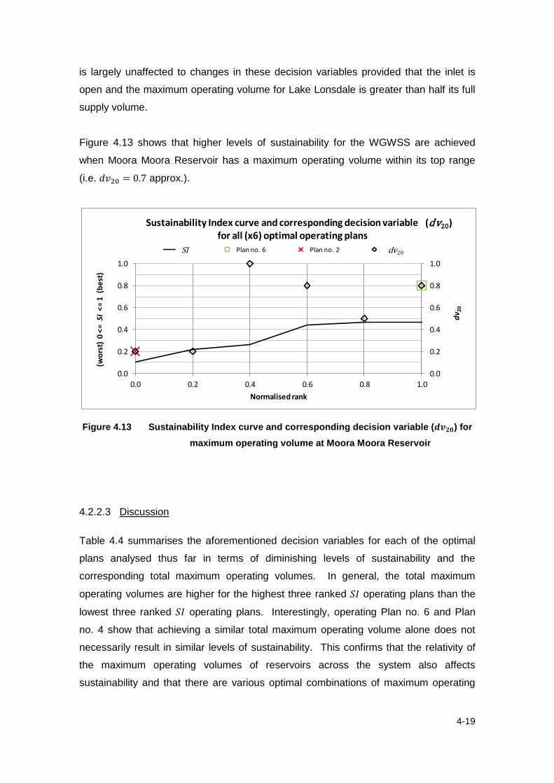
4-19
is largely unaffected to changes in these decision variables provided that the inlet is
open and the maximum operating volume for Lake Lonsdale is greater than half its full
supply volume.
Figure 4.13 shows that higher levels of sustainability for the WGWSS are achieved
when Moora Moora Reservoir has a maximum operating volume within its top range
(i.e. approx.).
Figure 4.13 Sustainability Index curve and corresponding decision variable ( ) for
maximum operating volume at Moora Moora Reservoir
4.2.2.3 Discussion
Table 4.4 summarises the aforementioned decision variables for each of the optimal
plans analysed thus far in terms of diminishing levels of sustainability and the
corresponding total maximum operating volumes. In general, the total maximum
operating volumes are higher for the highest three ranked operating plans than the
lowest three ranked operating plans. Interestingly, operating Plan no. 6 and Plan
no. 4 show that achieving a similar total maximum operating volume alone does not
necessarily result in similar levels of sustainability. This confirms that the relativity of
the maximum operating volumes of reservoirs across the system also affects
sustainability and that there are various optimal combinations of maximum operating
0.0
0.2
0.4
0.6
0.8
1.0
0.0
0.2
0.4
0.6
0.8
1.0
0.0 0.2 0.4 0.6 0.8 1.0
(wo
rst)
0 <
= S
I<
= 1
(b
est
)
Normalised rank
Sustainability Index curve and corresponding decision variable dv1 for all (x6) optimal operating plans
Ienv Plan no. 6 Plan no. 2 Ienvdv20
(dv20)
SI
dv 2
0

4-20
volumes for the DM to consider. In this instance, the for operating Plan no. 4 is less
than for Plan no. 6 due to the significant reductions in maximum operating volumes at
Toolondo Reservoir, Lake Bellfield, and Moora Moora Reservoir which are not able to
compensate for the increase in maximum operating volume at Taylors Lake. This
reduced performance of the WGWSS under Plan no. 4 is reflected in the lower levels of
reliability, resiliency, and vulnerability as depicted in Table 4.3 (i.e. Plan no. 6:
Plan no. 4: = 11.9%, = 9.6%,
= 2.8%).
Table 4.4 Storage maximum operating volumes (in ML) and Sustainability Index
(italics) for the six optimal operating plans for the lower order MOOP
It is also worth highlighting that Plan no. 5 and Plan no. 3 have greater total maximum
operating volumes than that under Plan no. 6. This suggests that increasing the total
maximum operating volume too high may have the effect of harvesting too much water
and not allowing high fresh flows to satisfy environmental water demands downstream.
4.2.3 Conclusions
Section 4.2 presented a lower order MOOP for the purposes of demonstrating the
effectiveness of the in terms of ranking optimal operating plans. The outcomes of
this analysis are summarised as follows:
The was shown to be a useful tool for evaluating and comparing optimal
operating plans with respect to the objective space and decision space. In
Decision variable
Plan no. 6 Plan no. 5 Plan no. 3 Plan no. 1 Plan no. 4 Plan no. 2
dv 14 (Toolondo Reservoir) 27,729 55,458 27729 73944 18,486 46,215
dv 16 (Lake Bellfield) 15,200 7,600 7600 15200 7,600 45,600
dv 17 (Taylors Lake) 16,850 20,220 10110 26960 26,960 10,110
dv 18 (Rocklands Reservoir) 208,800 348,000 278400 34800 208,800 34,800
dv 19 (Lake Lonsdale - via outlet) 52,000 52,000 58500 32500 52,000 65,000
dv 20 (Moora Moora Reservoir) 5,040 3,150 5040 6300 1,260 1,260
Total 325,619 486,428 387,379 189,704 315,106 202,985
Sustainability Index (SI ) 0.47 0.46 0.44 0.26 0.22 0.11
dv 15 i s not included as i t a lone does not represent a s torage maximum operating volume
Storage maximum operating volumes (ML)

4-21
terms of the objective space, ranking and plotting the against its normalised
rank provided a visual representation of the Pareto front. For the lower order
MOOP discussed, Plan no. 6 was the highest ranked operating plan (
) and Plan no. 2 was the lowest ranked operating plan ( ). In
terms of the decision space, the corresponding decision variable values were
plotted together with the curve and shown to inform the DM about how
different planning decisions influence a system’s sustainability.
The gradient of the curve was shown to represent the diversity of the
operating plans with respect to the objective space. For the lower order MOOP,
the gradient of the curve between Plan no. 3 and Plan no. 1 was greater than
that given between Plan no. 1 and Plan no. 4. It was shown that the average of
the crowding distances for Plan no. 3 and Plan no. 1 was greater than that
given by Plan no. 1 and Plan no. 4. Thus, the gradient of the curve provided
the DM with a sense of the diversity amongst the optimal operating plans along
the Pareto front.
It is important to mention that the lower order MOOP assumes that the sustainability of
the WGWSS can be quantified in terms of environmental interests only, and as such
ignores the implications of changes to the maximum operating volumes with respect to
non-environmental interests for water. This may cause the O-S model to find optimal
operating plans that have detrimental effects on other water users such as those
identified in this work (e.g. the significant reductions in maximum operating volume at
Lake Bellfield which would in all likelihood affect the supply to consumptive users via
the Wimmera Mallee Pipeline). This highlights the importance of problem formulation
and the need to take explicit account for all interests for water in order for the optimal
operating plans to be relevant in a real-world sense. Nonetheless, the outcomes of this
work demonstrate that the provides a convenient and simple means to rank optimal
operating plans with respect to many objectives and many optimal operating plans as
generally occurs in higher order MOOPs.
4.3 A series of higher order MOOPs – all user groups
The purpose of this section is to demonstrate the effectiveness of the as a means to
assess the level of influence a set of operating rules has on the sustainability of the
WGWSS. By understanding which planning decisions underpin the sustainability of the

4-22
system, the DM is aware of which operating rules are paramount in terms of the overall
operating plan. This information would be particularly useful in water resources
systems that have many complex operating rules which must be optimised in order to
maintain an agreed level of sustainability or to improve on current levels. This section
builds on the analysis of the lower order MOOP discussed in Section 4.2 which showed
that the could be used to rank optimal operating plans. The same principles
developed for that problem are applied to a series of higher order MOOPs which
consider the needs of all user groups in the WGWSS. Each O-S model run within the
series focuses on one group of planning decisions as defined by the six categories
given in Table 4.1. Run (A1), the higher order MOOP described in Section 3.3, is also
included in this analysis as it serves as a basis from which to evaluate each O-S model
run.
4.3.1 Problem formulation and model setup
The problem is to optimise the system operating rules with regards to 18 competing
objectives which consider environmental, social, consumptive, and system-wide
interests for water - refer to Equations 4.9 to 4.26. As explained in Section 3.3, the
problem is formulated based on the assumption that the sustainability of the WGWSS
is measured in terms of three performance metrics (i.e. reliability ( ), resiliency
( ), and vulnerability ( )) for the ith interest for water. Equations 4.9 to 4.11 relate
to three environmental ( ) interests for water expressed in terms of nil environmental
flow deficits, and are the same as Equations 4.6 to 4.8 in Section 4.2.1. Equations
4.12 to 4.20 relate to nine social ( ) interests for water expressed in terms of the
volume of the storage ( ) being Lake Lonsdale ( ), Lake Fyans ( ), and
Rocklands Reservoir ( ). Equations 4.21 to 4.23 relate to three consumptive ( )
interests for water expressed in terms of nil supply deficits. Equations 4.24 to 4.26
relate to three system-wide interests for water expressed in terms of water allocations
( ). The 18 objective functions are in direct conflict with each other both between
the various interests for water and within each interest for water. For instance,
increasing the performance of the environmental objectives means that there is less
water extracted from waterways which reduces the volume available for supply to
consumptive users and for provision of recreation amenity, and vice versa.
Additionally, within the environmental user group, an increase the reliability of nil
environmental flow deficits does not necessarily equate to an increase in resiliency; nor

4-23
does the increase in any or both of these two objectives (i.e. reliability and resiliency)
result in reduced vulnerability of such deficits, and vice versa.
(4.9)
(4.10)
(4.11)
, (4.12)
(4.13)
(4.14)
, (4.15)
(4.16)
(4.17)
, (4.18)
(4.19)
(4.20)
, (4.21)
(4.22)
(4.23)
, (4.24)
(4.25)
(4.26)
Where, ;
Subject to the constraints as configured in the revised Wimmera-Glenelg
REALM model (refer Section 3.3.2).
The decision variables to solve for are to as specified in Table 4.1.

4-24
The above higher order MOOPs are solved for five generations using the O-S
modelling approach with the following optimisation parameters:
(refer
Section 3.4.2.2 for further details regarding the optimisation parameters adopted).
In order to assess the level of influence a set of operating rules has on the
sustainability of the WGWSS, the 18-objective problem is used to solve for one
planning decision category at a time. The 24 planning decisions are categorised into 6
different areas of system operation related to priorities of supply; storage flood reserve
volumes; environmental allocation shares; flow paths; storage maximum operating
volumes; and storage draw down priorities and storage targets (refer Table 4.1). The
approach used to solve for a single planning decision category is based on the
assumption that the DM is interested in improving the current level of sustainability that
is achieved under the base case scenario (BC01) by optimising a planning decision
category. For this reason, the approach involves setting or fixing the decision
variables, for all but one of the categories, to the values used in BC01. In this way, the
problem is solved for the planning decisions that are not fixed i.e. the O-S model is able
to search for optimal operating plans with respect to that (single) set of operating rules
only. Table 4.5 sets out the O-S modelling runs undertaken as part of this investigation
showing which categories are fixed/not fixed to BC01 levels, denoted with “F” and “ F”
respectively. With the exception of Run (A1), this approach results in 6 runs (i.e. Run
(B1) to Run (G1)) which are similar to BC01 in all but one facet of system operation.
Run (A1) does not have any planning decisions fixed which means that the O-S model
is able to search for optimal operating plans with respect to all the operating rules (as
per the MOOP described in Section 3.3). In essence, BC01 represents the current
operating regime based on past operational experience, whereas the optimal operating
plans found under Run (A1) represent the possibility of new operating rules that
achieve a greater level of sustainability for the WGWSS.

4-25
Table 4.5 Settings of decision variables for optimisation-simulation modelling
scenarios Run (A1) to Run (G1)
Category of decision variable
Optimisation-simulation scenarios (bold) and corresponding setting
of decision variables (F = fixed, NF = not fixed)
Run (A1)
Run (B1)
Run (C1)
Run (D1)
Run (E1)
Run (F1)
Run (G1)
Priority of supply ( to ) NF NF F F F F F
Flood reserve volume ( ) NF F NF F F F F
Share of environmental allocation ( to )
NF F F NF F F F
Flow path ( and ) NF F F F NF F F
Storage maximum operating volume ( to )
NF F F F F NF F
Storage draw down priority and storage target ( to )
NF F F F F F NF
‘ F’ refers to decision variables values which are not fixed to those under base case scenario (BC01). ‘F’ refers to decision variables values which are fixed to those under base case scenario (BC01).
4.3.2 Modelling results and discussion
4.3.2.1 Objective space
For each of the modelling scenarios described in Table 4.5 (i.e. Run (A1) to Run (G1)),
the O-S model was run for five generations as for the lower order MOOP (refer to
Section 4.2) and the population with the highest ranked operating plan was selected
for analysis. The O-S model found 56, 29, 49, 48, 6, 49, and 49 optimal operating
plans forming the Pareto front for each of the seven scenarios from Run (A1) to Run
(G1) respectively. As shown in Section 4.2, the visualisation of the Pareto front is
relatively simple in lower order MOOPs whereas for the present higher order MOOP,
using a two-dimensional Cartesian coordinate plane would be a tedious exercise
resulting in 153 different combinations ( ) of the 18 objective functions considered i.e.
18
. However, Figure 4.14 demonstrates the convenience of
summarising the optimal operating plans using the curve for the seven modelling
scenarios. Based on the outcomes of the lower order MOOP, the gradient of the
curve represents the diversity of the operating plans with respect to the objective
space. A larger gradient represents operating plans which are more diverse than those
that produce a section of curve with a smaller gradient. The curves in Figure 4.14
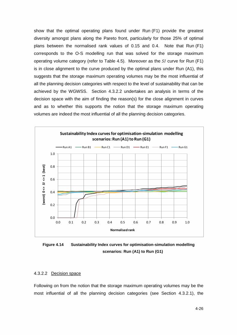
4-26
show that the optimal operating plans found under Run (F1) provide the greatest
diversity amongst plans along the Pareto front, particularly for those 25% of optimal
plans between the normalised rank values of 0.15 and 0.4. Note that Run (F1)
corresponds to the O-S modelling run that was solved for the storage maximum
operating volume category (refer to Table 4.5). Moreover as the curve for Run (F1)
is in close alignment to the curve produced by the optimal plans under Run (A1), this
suggests that the storage maximum operating volumes may be the most influential of
all the planning decision categories with respect to the level of sustainability that can be
achieved by the WGWSS. Section 4.3.2.2 undertakes an analysis in terms of the
decision space with the aim of finding the reason(s) for the close alignment in curves
and as to whether this supports the notion that the storage maximum operating
volumes are indeed the most influential of all the planning decision categories.
Figure 4.14 Sustainability Index curves for optimisation-simulation modelling
scenarios: Run (A1) to Run (G1)
4.3.2.2 Decision space
Following on from the notion that the storage maximum operating volumes may be the
most influential of all the planning decision categories (see Section 4.3.2.1), the
0.0
0.2
0.4
0.6
0.8
1.0
0.0 0.1 0.2 0.3 0.4 0.5 0.6 0.7 0.8 0.9 1.0
(wo
rst)
0 <
= S
I<
= 1
(b
est
)
Normalised rank
Sustainability Index curves for optimisation-simulation modelling scenarios: Run (A1) to Run (G1)
Run A1 Run B1 Run C1 Run D1 Run E1 Run F1 Run G1

4-27
analysis of the O-S modelling results focuses on the values of to with the aim
of finding conclusive evidence that the storage maximum operating volumes are the
most influential of all the planning decision categories. The decision variable values
( to ) for all 49 optimal operating plans under Run (F1) are compared to the
values of the 56 optimal plans under Run (A1) using their corresponding curve.
Figure 4.15 shows the values for decision variable for all optimal operating plans
together with their corresponding curve under Run (A1) and Run (F1) respectively.
Whilst Figure 4.15 provides a means to investigate the effect of a decision variable
value on the sustainability of the system (in terms of ), these figures do not provide a
direct comparison of the distribution of values for all optimal operating plans under Run
(A1) and Run (F1). The distribution of values here refers to the number of decision
variable values that pertain to a particular class within the range of the decision
variable. Understanding the distribution of decision variable values informs the DM of
how such values contribute to higher levels of sustainability of the WGWSS. For this
purpose, the relative frequency distribution of the decision variable values can be used
to bring both sets of data together.
Figure 4.15 Sustainability Index curve and corresponding decision variable ( ) for
maximum operating volume at Rocklands Reservoir - Run (A1) and Run (F1)
0.0
0.2
0.4
0.6
0.8
1.0
0.0
0.2
0.4
0.6
0.8
1.0
0.0 0.1 0.2 0.3 0.4 0.5 0.6 0.7 0.8 0.9 1.0
(wo
rst)
0 <
= S
I<
= 1
(b
est
)
Normalised rank
Sustainability Index curve and corresponding decision variable for all optimal operating plans - Run (A1) and Run (F1)
Ienv Ienv Ienv Ienvdv18 - Run (A1)
(dv18)
SI - Run (A1)
dv 1
8
SI - Run (F1) dv18 - Run (F1)

4-28
The relative frequency in this case is defined as the number of decision variable values
that pertain to a particular class within the range of the decision variable divided by the
total number of decision variables in the whole range. For instance, Figure 4.15 shows
that there are 2 out of 56 optimal operating plans under Run (A1) which have a
value of (i.e.
). Figure 4.16 shows the relative frequency distribution of
decision variable under both Run (A1) and Run (F1). It also shows that the
largest disparity in occurs for values 0.1 and 0.2. Figure 4.15 shows that a value
of 0.2 in generally has the effect of contributing to an increase in the whereas a
value of 0.1 has the opposite effect.
Figure 4.16 Relative frequency distribution of decision variable ( ) maximum
operating volume at Rocklands Reservoir - Run (A1) and Run (F1)
The remaining storage maximum operating volumes (i.e. to , , and )
are analysed in the same way; by focusing on the largest disparity between
corresponding decision variable values under Run (A1) and Run (F1) in order to
explain how individual maximum operating volumes contribute to higher levels of
sustainability of the WGWSS. In Section 4.2.2.2, the decision variables corresponding
to the storage maximum operating volumes for Rocklands Reservoir, Toolondo
Reservoir, and Taylors Lake (i.e. , , and ) were analysed together as
these storages are generally operated as a sub-system of the WGWSS. Toolondo
Reservoir is primarily used as a balancing storage in order to maximise the harvesting
0
10
20
30
0.0 0.1 0.2 0.3 0.4 0.5 0.6 0.7 0.8 0.9 1.0
Re
lati
ve fr
eq
ue
ncy
(%)
Relative frequency distribution of decision variable dv1 for all optimal operating plans - Run (A1) and Run (F1)
Run (A1) Run (F1)
dv 18
(dv18)

4-29
of flows from the upper Glenelg River at Rocklands Reservoir with transfers to Taylors
Lake downstream of Toolondo Reservoir (refer Figure 4.1). Figure 4.17 and Figure
4.18 compare the decision variable values for the storage maximum operating volume
for Toolondo Reservoir (i.e. ) under Run (A1) and Run (F1) using the curve and
the relative frequency distribution respectively. The results for Toolondo Reservoir
Figure 4.17 Sustainability Index curve and corresponding decision variable ( ) for
maximum operating volume at Toolondo Reservoir - Run (A1) and Run (F1)
Figure 4.18 Relative frequency distribution of decision variable ( ) maximum
operating volume at Toolondo Reservoir - Run (A1) and Run (F1)
0.0
0.2
0.4
0.6
0.8
1.0
0.0
0.2
0.4
0.6
0.8
1.0
0.0 0.1 0.2 0.3 0.4 0.5 0.6 0.7 0.8 0.9 1.0
(wo
rst)
0 <
= S
I<
= 1
(b
est
)
Normalised rank
Sustainability Index curve and corresponding decision variable for all optimal operating plans - Run (A1) and Run (F1)
Ienv Ienv Ienv Ienvdv14 - Run (A1)
(dv14)
SI - Run (A1)
dv 1
4
SI - Run (F1) dv14 - Run (F1)
0
10
20
30
0.0 0.1 0.2 0.3 0.4 0.5 0.6 0.7 0.8 0.9 1.0
Re
lati
ve fr
eq
ue
ncy
(%)
Relative frequency distribution of decision variable dv1 for all optimal operating plans - Run (A1) and Run (F1)
Run (A1) Run (F1)
dv 14
(dv14)

4-30
show that the largest disparity in variable value is for , where this value is
used in eight optimal operating plans under Run (A1) and in one optimal plan under
Run (F1). In general, the results show that optimal operating plans that have a
value of 0.9 contribute to higher levels of sustainability for the WGWSS. Figure 4.19
and Figure 4.20 compare the decision variable values for Taylors Lake (i.e. ) using
Figure 4.19 Sustainability Index curve and corresponding decision variable ( ) for
maximum operating volume at Taylors Lake - Run (A1) and Run (F1)
Figure 4.20 Relative frequency distribution of decision variable ( ) maximum
operating volume at Taylors Lake - Run (A1) and Run (F1)
0.0
0.2
0.4
0.6
0.8
1.0
0.0
0.2
0.4
0.6
0.8
1.0
0.0 0.1 0.2 0.3 0.4 0.5 0.6 0.7 0.8 0.9 1.0
(wo
rst)
0 <
= S
I<
= 1
(b
est
)
Normalised rank
Sustainability Index curve and corresponding decision variable for all optimal operating plans - Run (A1) and Run (F1)
Ienv Ienv Ienv Ienvdv17 - Run (A1)
(dv17)
SI - Run (A1)
dv 1
7
SI - Run (F1) dv17 - Run (F1)
0
10
20
0.0 0.1 0.2 0.3 0.4 0.5 0.6 0.7 0.8 0.9 1.0
Re
lati
ve fr
eq
ue
ncy
(%)
Relative frequency distribution of decision variable dv1 for all optimal operating plans - Run (A1) and Run (F1)
Run (A1) Run (F1)
dv 17
(dv17)

4-31
the curve and the relative frequency distribution respectively. The results for Taylors
Lake show that the largest disparity in variable value is for , where this value
is used in seven optimal operating plans under Run (A1) and in none of the optimal
plans under Run (F1). In general, the results show that optimal operating plans that
use a value of 0.4 contribute to an increase in the sustainability level of the
WGWSS.
Overall, the results for Rocklands Reservoir, Toolondo Reservoir, and Taylors Lake
indicate that higher values of the corresponding decision variables contribute to higher
levels of sustainability of the WGWSS.
Lake Bellfield is the primary source of supply to consumptive users (19) to (30) and is
operated at FSV except over the April to September period when it is lowered to 97%
of FSV for dam safety reasons and to manage flood flows (see Figure 4.1). Figure
4.21 and Figure 4.22 compare the decision variable values for the storage maximum
operating volume for Lake Bellfield (i.e. ) using the curve and the relative
frequency distribution respectively. The results show that the disparity in is
relatively uniform across all values and that there is no obvious pattern in terms of how
certain values of this decision variable contribute to higher levels of sustainability of the
WGWSS.
Figure 4.21 Sustainability Index curve and corresponding decision variable ( ) for
maximum operating volume at Lake Bellfield - Run (A1) and Run (F1)
0.0
0.2
0.4
0.6
0.8
1.0
0.0
0.2
0.4
0.6
0.8
1.0
0.0 0.1 0.2 0.3 0.4 0.5 0.6 0.7 0.8 0.9 1.0
(wo
rst)
0 <
= S
I<
= 1
(b
est
)
Normalised rank
Sustainability Index curve and corresponding decision variable for all optimal operating plans - Run (A1) and Run (F1)
Ienv Ienv Ienv Ienvdv16 - Run (A1)
(dv16)
SI - Run (A1)
dv 1
6
SI - Run (F1) dv16 - Run (F1)

4-32
Figure 4.22 Relative frequency distribution of decision variable ( ) maximum
operating volume at Lake Bellfield - Run (A1) and Run (F1)
As explained in Section 4.2.2.2, there are two decision variables that control the
maximum operating volume at Lake Lonsdale. Decision variable controls the flow
of water entering the storage and has a value of either 0 or 1, where 0 means that the
inlet is completely closed and 1 represents a fully opened inlet. Decision variable
controls the storage operating volume and has a value between 0 and 1, where 0
means that the storage is effectively not used or decommissioned and 1 represents a
maximum operating volume at FSV.
Figure 4.23 and Figure 4.24 compare the decision variable values for the inlet at Lake
Lonsdale (i.e. ) using the curve and the relative frequency distribution
respectively. The results for the inlet show that there are more optimal operating plans
that use a value of 0 for under Run (A1) than those under Run (F1). That is, a
greater number of optimal operating plans use values of 0.1, 0.3, 0.4, 0.5, and 0.6
under Run (A1) compared to those under Run (F1). The results for both decision
variables ( and ) indicate that values which represent a closed inlet together
with lower maximum operating volumes contribute to higher levels of sustainability of
the WGWSS.
0
10
20
0.0 0.1 0.2 0.3 0.4 0.5 0.6 0.7 0.8 0.9 1.0
Re
lati
ve fr
eq
ue
ncy
(%)
Relative frequency distribution of decision variable dv1 for all optimal operating plans - Run (A1) and Run (F1)
Run (A1) Run (F1)
dv 16
(dv16)

4-33
Figure 4.23 Sustainability Index curve and corresponding decision variable ( ) for
maximum operating volume at Lake Lonsdale (inlet) - Run (A1) and Run (F1)
Figure 4.24 Relative frequency distribution of decision variable ( ) maximum
operating volume at Lake Lonsdale (inlet) - Run (A1) and Run (F1)
0.0
0.2
0.4
0.6
0.8
1.0
0.0
0.2
0.4
0.6
0.8
1.0
0.0 0.1 0.2 0.3 0.4 0.5 0.6 0.7 0.8 0.9 1.0
(wo
rst)
0 <
= S
I<
= 1
(b
est
)
Normalised rank
Sustainability Index curve and corresponding decision variable for all optimal operating plans - Run (A1) and Run (F1)
Ienv Ienv Ienv Ienvdv15 - Run (A1)
(dv15)
SI - Run (A1)
dv 1
5
SI - Run (F1) dv15 - Run (F1)
0
10
20
30
40
50
60
0.0 0.1 0.2 0.3 0.4 0.5 0.6 0.7 0.8 0.9 1.0
Re
lati
ve fr
eq
ue
ncy
(%)
Relative frequency distribution of decision variable dv1 for all optimal operating plans - Run (A1) and Run (F1)
Run (A1) Run (F1)
dv 15
(dv15)

4-34
Figure 4.25 and Figure 4.26 compare the decision variable values for the storage
maximum operating volume for Lake Lonsdale (i.e. ) using the curve and the
relative frequency distribution respectively. The results generally show that there are
more optimal operating plans that use lower values of under Run (A1) than those
under Run (F1).
Figure 4.25 Sustainability Index curve and corresponding decision variable ( ) for
maximum operating volume at Lake Lonsdale (outlet) - Run (A1) and Run (F1)
Figure 4.26 Relative frequency distribution of decision variable ( ) maximum
operating volume at Lake Lonsdale (outlet) - Run (A1) and Run (F1)
0.0
0.2
0.4
0.6
0.8
1.0
0.0
0.2
0.4
0.6
0.8
1.0
0.0 0.1 0.2 0.3 0.4 0.5 0.6 0.7 0.8 0.9 1.0
(wo
rst)
0 <
= S
I<
= 1
(b
est
)
Normalised rank
Sustainability Index curve and corresponding decision variable for all optimal operating plans - Run (A1) and Run (F1)
Ienv Ienv Ienv Ienvdv19 - Run (A1)
(dv19)
SI - Run (A1)
dv 1
9
SI - Run (F1) dv19 - Run (F1)
0
10
20
0.0 0.1 0.2 0.3 0.4 0.5 0.6 0.7 0.8 0.9 1.0
Re
lati
ve fr
eq
ue
ncy
(%)
Relative frequency distribution of decision variable dv1 for all optimal operating plans - Run (A1) and Run (F1)
Run (A1) Run (F1)
dv 19
(dv19)

4-35
Figure 4.27 and Figure 4.28 compare the decision variable values for the storage
maximum operating volume for Moora Moora Reservoir (i.e. ) using the curve
and the relative frequency distribution respectively. The results show that the disparity
in the two runs in is relatively uniform across all values and that there is no
obvious pattern in terms of how certain values of this decision variable contribute to
Figure 4.27 Sustainability Index curve and corresponding decision variable ( ) for
maximum operating volume at Moora Moora Reservoir - Run (A1) and Run (F1)
Figure 4.28 Relative frequency distribution of decision variable ( ) maximum
operating volume at Moora Moora Reservoir - Run (A1) and Run (F1)
0.0
0.2
0.4
0.6
0.8
1.0
0.0
0.2
0.4
0.6
0.8
1.0
0.0 0.1 0.2 0.3 0.4 0.5 0.6 0.7 0.8 0.9 1.0
(wo
rst)
0 <
= S
I<
= 1
(b
est
)
Normalised rank
Sustainability Index curve and corresponding decision variable for all optimal operating plans - Run (A1) and Run (F1)
Ienv Ienv Ienv Ienvdv20 - Run (A1)
(dv20)
SI - Run (A1)
dv 2
0
SI - Run (F1) dv20 - Run (F1)
0
10
20
0.0 0.1 0.2 0.3 0.4 0.5 0.6 0.7 0.8 0.9 1.0
Re
lati
ve fr
eq
ue
ncy
(%)
Relative frequency distribution of decision variable dv1 for all optimal operating plans - Run (A1) and Run (F1)
Run (A1) Run (F1)
dv 20
(dv20)

4-36
higher levels of sustainability of the WGWSS.
4.3.2.3 Discussion
The results presented in Sections 4.3.2.1 and 4.3.2.2 show that the effect of decision
variables to is varied with respect to their effect on the sustainability of the
WGWSS (in terms of ). For instance, the combined effect of higher storage
maximum operating volumes for Rocklands Reservoir, Toolondo Reservoir, and
Taylors Lake contribute to higher levels of sustainability (i.e. , , and ).
Interestingly the combined effect of decision variables for Lake Lonsdale (i.e. and
) show that there is an increase in the system’s sustainability with the inlet
completely closed together with a decrease in the maximum operating volume. Both
sets of results indicate that the O-S model has found optimal operating plans that
balance the harvesting of water and the needs of users between the storages located
in western parts of the WGWSS (i.e. Rocklands Reservoir, Toolondo Reservoir and
Taylors Lake) and those in the eastern parts (i.e. Lake Lonsdale and to a lesser extent
Lake Bellfield). This balancing approach is a feature of the current operating regime as
it has worked successfully since 1966 when the last headworks storage, Lake Bellfield,
was completed (Barlow, 1987; GWMWater, 2011).
The results for Lake Bellfield and Moora Moora Reservoir showed that there were no
obvious patterns for how certain values of the corresponding decision variables
contributed to higher levels of system sustainability (i.e. and ). Such results
suggest that the DM would have a greater degree of flexibility in terms of the operation
of Lake Bellfield and Moora Moora Reservoir with respect to maintaining/improving the
sustainability of the WGWSS. This flexibility would benefit all users, particularly in the
case of Lake Bellfield which is currently the primary source of supply to consumptive
users (19) to (30) (refer Figure 4.1) and is also a popular tourist destination given its
recreation amenity (e.g. fishing, boating, camping etc). However the current practice is
to operate Lake Bellfield at FSV except over the April to September period when it is
lowered to 97% of FSV for dam safety reasons and to manage flood flows. The reason
for this is to ensure that the consumptive users receive an acceptable level of water
quality which is often better at Lake Bellfield than that downstream at Lake Lonsdale
and Taylors Lake. As such water quality considerations have not been included in the
MOOP as an objective function (for Lake Bellfield), it is suggested that any major
changes to the storage maximum operating volume for Lake Bellfield be further

4-37
investigated in terms of the effect that different sources of water have on supplies to
the consumptive users.
In a similar discussion to that for the lower order MOOP in Section 4.2.2.3, the results
of the higher order MOOP may also be discussed in terms of the sum of the individual
storage maximum operating volumes for Toolondo Reservoir, Lake Bellfield, Taylors
Lake, Rocklands Reservoir, Lake Lonsdale, and Moora Moora Reservoir. Figure 4.29
compares the total maximum operating volumes for all optimal operating plans under
Run (A1) and Run (F1) using the curve. The results for both runs show that higher
total maximum operating volumes generally contribute to higher levels of sustainability
of the WGWSS. Note that this outcome is the same as that for the lower order MOOP
which considered three environmental objectives.
Figure 4.29 Sustainability Index curve and corresponding total maximum operating
volume for all optimal operating plans - Run (A1) and Run (F1)
Figure 4.30 compares the total maximum operating volumes for all optimal operating
plans under Run (A1) and Run (F1) in terms of their relative frequency distribution.
With respect to the 100 GL class interval considered, the results show that the relative
frequency distribution of total maximum operating volumes between both runs is
relatively uniform. This means that both runs have very similar optimal operating plans
in terms of the number of plans that specify a similar total maximum operating volume.
This similarity in results together with the close alignment of the curve for Run (F1)
100
200
300
400
500
600
0.0
0.2
0.4
0.6
0.8
1.0
0.0 0.1 0.2 0.3 0.4 0.5 0.6 0.7 0.8 0.9 1.0
(wo
rst)
0 <
= S
I<
= 1
(b
est
)
Normalised rank
Sustainability Index curve and corresponding total maximum operating volume for all optimal operating plans - Run (A1) and Run (F1)
Ienv Ienv Ienv IenvMOVtot - Run (A1)SI - Run (A1)
Tota
l max
imu
m o
pe
rati
ng
vo
lum
e, M
OV
tot(G
L)
SI - Run (F1) MOVtot - Run (F1)

4-38
with Run (A1) (refer to Figure 4.14), provides conclusive evidence that the maximum
operating volumes are indeed the most influential of all the planning decision
categories with respect to the level of sustainability of the WGWSS. Had there instead
been a disparity between the relative frequency distribution between both runs, the
results would have indicated that there were other operating rules (from at least one
other planning decision category) which worked in combination with the storage
maximum operating volumes in order to achieve an curve in close alignment to
Run (A1). This important information means that the DM is able to focus more
attention on those operating rules which have the greatest impact on improving or
maintaining a desired level of sustainability.
Figure 4.30 Relative frequency distribution of total maximum operating volumes for all
optimal operating plans - Run (A1) and Run (F1)
Whilst the results in Figure 4.14 and Figure 4.30 show that the storage maximum
operating volumes are the most influential of all the planning decisions considered (in
terms of ), it is important to highlight that this does not mean that the other planning
decisions are not as important (as the storage maximum operating volumes). Evidence
of this is given by the fact that the curve for Run (F1) is not exactly the same as that
for Run (A1). This difference means that the other (less influential) planning decisions
play a part in contributing to higher levels of sustainability of the WGWSS. It is for this
0
10
20
30
40
0 - 100 100 - 200 200 - 300 300 - 400 400 - 500 500 - 600
Re
lati
ve fr
eq
ue
ncy
(%)
Relative frequency distribution of total maximum operating volumesfor all optimal operating plans - Run (A1) and Run (F1)
Run (A1) Run (F1)
Total maximum operating volume (GL)

4-39
reason, that all planning decisions considered thus far are included in the higher order
MOOPs presented in Section 4.4 and Chapter 5.
4.3.3 Conclusions
Section 4.3 presented a higher order MOOP for the purposes of demonstrating the
effectiveness of the as a means to assess the level of influence a set of operating
rules has on the sustainability of the WGWSS. A total of 24 planning decisions were
categorised into six different sets of operating rules and the O-S model was run to
solve the 18-objective problem, one planning decision category at a time. The six
planning decision categories related to priorities of supply (Run B1); storage flood
reserve volumes (Run C1); environmental allocation shares (Run D1); flow paths (Run
E1); storage maximum operating volumes (Run F1); and storage draw down priorities
and storage targets (Run G1) - refer to Table 4.1 for further details. As Run (A1) was
used to solve for all six planning decision categories in a single O-S model run, it was
used as a point of comparison representing the highest levels of sustainability in terms
of . The outcomes of this analysis are summarised as follows:
The was shown to be a useful tool for comparing optimal operating plans for
multiple modelling scenarios. In the objective space analysis, the curve was
used to compare the optimal plans found under the seven O-S modelling
scenarios on a single chart. The alternative two-dimensional plotting approach
would have resulted in 153 different charts each with a total of 286 optimal
plans which would have been a tedious task to analyse. Comparing the
curves against Run (A1), showed that the optimal operating plans found under
Run (F1) were in close alignment to Run (A1) and that the plans under Run (F1)
were the most diverse of all runs, particularly for those 25% of optimal plans
between the normalised rank values of 0.15 and 0.4. Note that Run (F1) relates
to the storage maximum operating volumes of Rocklands Reservoir, Toolondo
Reservoir, Taylors Lake, Lake Lonsdale, Lake Bellfield, and Moora Moora
Reservoir.
The decision space analysis compared Run (F1) against Run (A1) using the
curve and the relative frequency distribution of decision variable values. The
decision variable values of optimal operating plans under Run (F1) showed that
the effect of such values, in terms of the sustainability of the WGWSS, was

4-40
varied for the storages considered. The results showed that higher maximum
operating volumes for some storages contributed to higher levels of
sustainability (e.g. Rocklands Reservoir), while in other cases lower maximum
operating volumes had the same effect on sustainability (e.g. Lake Lonsdale).
The was shown to be a useful tool for assessing the influence of operating
rules on the sustainability of the WGWSS. This was demonstrated by
comparing the results of Run (F1) to Run (A1) in terms of the close alignment of
the curves and the relative frequency distribution of decision variable values.
Together, both sets of results confirmed that the storage maximum operating
volumes were the most influential of all the planning decision categories with
respect to the level of sustainability of the WGWSS.
Whilst the results showed that the storage maximum operating volumes were the most
influential of all the planning decisions considered (in terms of ), it was pointed out
that it did not mean that the other planning decisions were any less important than the
storage maximum operating volumes. Evidence of this was given by the fact that the
curve for Run (F1) was not exactly the same as that for Run (A1). This difference
meant that the other (less influential) planning decisions played a part in contributing to
higher levels of sustainability of the WGWSS. It was explained that this was the reason
for continuing to include all (six) planning decision categories as part of the higher
order MOOPs in Section 4.4 and Chapter 5.
Section 4.3 has shown that by understanding which planning decisions underpin the
sustainability of the system, the DM is informed of which operating rules are paramount
in terms of the overall operating plan. Additionally, higher levels of diversity in the
plans along the Pareto front means that the DM has a wider range of optimal plans to
choose from should there be a need to modify the current operating plan in order to
maintain an agreed level of sustainability or to improve on current levels. It is worth
highlighting that such comparative information, in relation to the effect of planning
decisions on sustainability levels, is not readily available to the DM at present time.
This is particularly important in the WGWSS as the interconnected nature of the
headworks means that there is the possibility to develop new, and potentially better,
operating plans that increase the sustainability of the system.

4-41
4.4 A higher order MOOP for the Wimmera-Glenelg Water Supply System – all user groups
So far the has been shown to be a useful tool for analysing optimal operating plans
along the Pareto front. In Section 4.2, the was used to rank optimal plans for a
lower order MOOP. Section 4.3 incorporated the in an investigation of various
higher order MOOPs in order to assess the level of influence different planning
decisions had on the sustainability of the WGWSS. The purpose of Section 4.4 is to
apply this understanding of the and to show the effect an optimal operating plan has
on four interests for water in the WGWSS. The four interests for water are expressed
in terms of their corresponding and are broadly classified into environmental ( ),
social ( ), consumptive ( ), and system-wide interests ( ) - refer to
Equations 4.1 to 4.4 for details regarding the calculation of the four values.
Section 4.4 does not introduce any additional O-S model runs; instead it investigates
two optimal operating plans under Run (A1). Run (A1) is the higher order MOOP of the
WGWSS which was described in Section 3.3 and was later used as a point of
reference in the analysis of the higher order MOOPs in Section 4.3. In order to
appreciate the full range of optimal operating plans that have been found, the two plans
analysed correspond to those that achieve the highest and lowest . These operating
plans are compared to the base case operating plan (BC01) in order to show the effect
of different combinations of operating rules on the four interests for water.
4.4.1 Problem formulation and model setup
Whilst the higher order MOOP referred to as ‘Run (A1)’ has already been presented in
Section 4.3.1, the problem is briefly described again for the reader’s convenience and
for completeness of Section 4.4. The problem for Run (A1) is to optimise the system
operating rules for the WGWSS with regards to 18 competing objectives which
consider environmental, social, consumptive, and system-wide interests for water -
refer to Equations 4.9 to 4.26 in Section 4.3.1. As explained in Section 3.3, the
problem is formulated based on the assumption that the sustainability of the WGWSS
is measured in terms of three performance metrics (i.e. reliability, resiliency, and
vulnerability) concerning the above four interests for water.

4-42
4.4.2 Modelling results and discussion
4.4.2.1 Objective space
As explained for Run (A1) in Section 4.3, the O-S model was run for five generations
and the population with the highest ranked operating plan was selected for analysis.
The O-S model found a total of 56 optimal operating plans forming the Pareto front.
Figure 4.31 shows the corresponding value for each optimal plan against its
normalised rank. The curve shows that the highest ranked operating plan is Plan
no. 11 (shown with a green square marker) and that one of the lowest ranked
operating plans is Plan no. 6 (shown with a red cross marker). Following the O-S
modelling procedure, the dominance test was performed on the 56 optimal plans and
the base case operating plan (BC01) in order to determine the status of BC01 (refer
Equation 2.2 for further details regarding the possible outcomes from the dominance
test). The test concluded that BC01 was not dominated by any of the 56 optimal plans
under Run (A1) and was therefore an optimal operating plan. Given this outcome,
BC01 is included in the curve as a point of reference (shown with a black open circle
marker) and is not to be confused with the 56 optimal plans that were found by the O-S
model under Run (A1).
Figure 4.31 Sustainability Index curve for all (x56) optimal operating plans under
Run (A1)
0.0
0.1
0.2
0.3
0.4
0.5
0.6
0.7
0.8
0.9
1.0
0.0 0.1 0.2 0.3 0.4 0.5 0.6 0.7 0.8 0.9 1.0
(wo
rst)
0 <
= S
I<
= 1
(b
est
)
Normalised rank
Sustainability Index curve for all (x56) optimal operating plans under Run (A1)
SI BC01 Plan no. 11 Plan no. 6SI
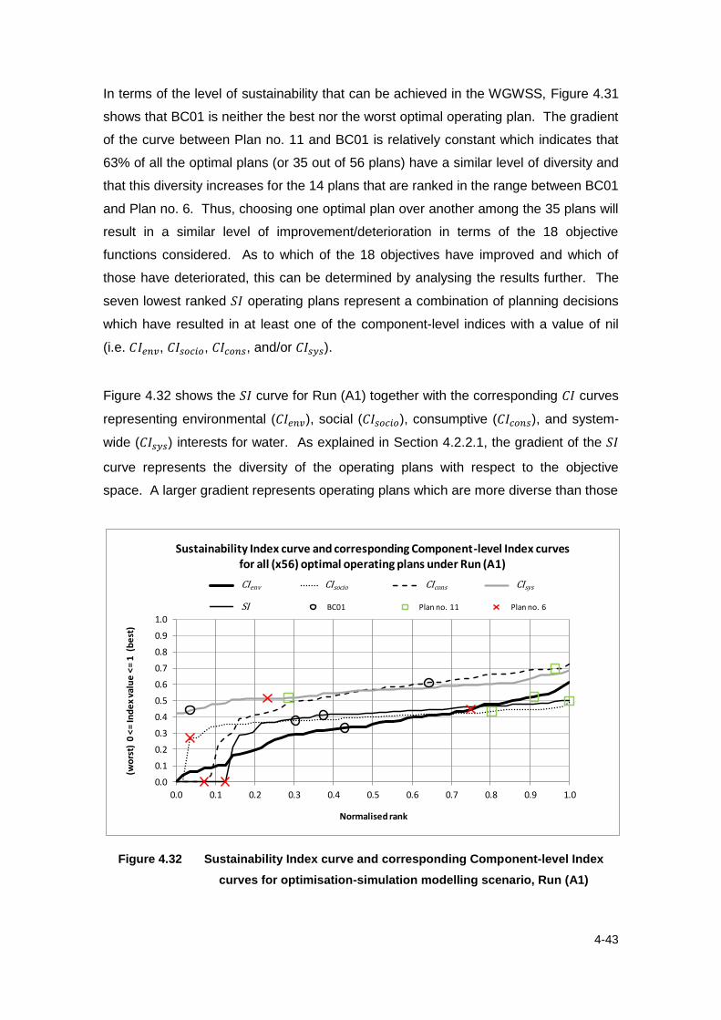
4-43
In terms of the level of sustainability that can be achieved in the WGWSS, Figure 4.31
shows that BC01 is neither the best nor the worst optimal operating plan. The gradient
of the curve between Plan no. 11 and BC01 is relatively constant which indicates that
63% of all the optimal plans (or 35 out of 56 plans) have a similar level of diversity and
that this diversity increases for the 14 plans that are ranked in the range between BC01
and Plan no. 6. Thus, choosing one optimal plan over another among the 35 plans will
result in a similar level of improvement/deterioration in terms of the 18 objective
functions considered. As to which of the 18 objectives have improved and which of
those have deteriorated, this can be determined by analysing the results further. The
seven lowest ranked operating plans represent a combination of planning decisions
which have resulted in at least one of the component-level indices with a value of nil
(i.e. , , , and/or ).
Figure 4.32 shows the curve for Run (A1) together with the corresponding curves
representing environmental ( ), social ( ), consumptive ( ), and system-
wide ( ) interests for water. As explained in Section 4.2.2.1, the gradient of the
curve represents the diversity of the operating plans with respect to the objective
space. A larger gradient represents operating plans which are more diverse than those
Figure 4.32 Sustainability Index curve and corresponding Component-level Index
curves for optimisation-simulation modelling scenario, Run (A1)
0.0
0.1
0.2
0.3
0.4
0.5
0.6
0.7
0.8
0.9
1.0
0.0 0.1 0.2 0.3 0.4 0.5 0.6 0.7 0.8 0.9 1.0
(wo
rst)
0 <
= In
de
x va
lue
<=
1 (
be
st)
Normalised rank
Sustainability Index curve and corresponding Component-level Index curves for all (x56) optimal operating plans under Run (A1)
Ienv Isocio Icons Isys
SI BC01 Plan no. 11 Plan no. 6
CIenv CIsocio CIcons CIsys
SI

4-44
that produce a section of curve with a smaller gradient. The same principle can be
applied to the curve except that the diversity of operating plans relates to a single
interest for water. For instance, the diversity of plans in terms of system-wide interests
is relatively constant compared to the diversity of plans in terms of consumptive
interests, particularly for those 40% of optimal plans between the normalised rank
values of 0 and 0.4. Table 4.6 is a summary of the objective function ( ) values,
values, and values for BC01, Plan no. 11, and Plan no. 6.
Table 4.6 Objective function values, Component-level Index values, and
Sustainability Index values for the base case operating plan (BC01) and
for two optimal operating plans under Run (A1) i.e. Plan no. 11 - highest
ranked operating plan, and Plan no. 6 - lowest ranked operating plan
‘ ’ refers to objective function which is defined in Section 4.3.1. ‘ ’ refers to the Component-level Index for the i
th interest for water as defined in Section 4.1.
‘ ’ refers to the Sustainability Index for the Wimmera-Glenelg Water Supply System as defined in Equation 4.5. ‘ ’ refer to the maximisation or minimisation of as defined in Equations 4.9 to 4.26. ‘ ’ refer to the reliability, resiliency, and vulnerability performance metrics respectively, as defined in Section 3.2.4.
‘ ’ refers to environmental interests for water as defined in Section 3.2.3.1. ‘ ’ refer to social interests for water at Lake Lonsdale, Lake Fyans, and Rocklands Reservoir respectively, as defined in Section 3.2.3.2.
‘ ’ refers to consumptive interests for water as defined in Section 3.2.3.3. ‘ ’ refers to system-wide interests for water as defined in Section 3.2.3.4.
BC01Run (A1)
- Plan no. 11
Run (A1)
- Plan no. 6
Max, f 1 = Rel env Reliability of nil environmental flow deficits - Equation (4.9) 25% 38% 38%
Max, f 2 = Res env Resiliency of nil environmental flow deficits - Equation (4.10) 16% 38% 25%
Min, f 3 = Vul env Vulnerability of environmental flow deficits - Equation (4.11) 10% 2% 4%
CI env Environmental Component-level Index - Equation (4.1) 0.33 0.52 0.45
Max, f 4 = Rel LL Reliability of volume at Lake Lonsdale exceeding 5,379 ML - Equation (4.12) 61% 92% 70%
Max, f 5 = Res LL Resiliency of volume at Lake Lonsdale exceeding 5,379 ML - Equation (4.13) 8% 3% 8%
Min, f 6 = Vul LL Vulnerability of volume at Lake Lonsdale falling below 5,379 ML - Equation (4.14) 26% 13% 23%
Max, f 7 = Rel LF Reliability of volume at Lake Fyans exceeding 1,761 ML - Equation (4.15) 99% 100% 93%
Max, f 8 = Res LF Resiliency of volume at Lake Fyans exceeding 1,761 ML - Equation (4.16) 33% 100% 1%
Min, f 9 = Vul LF Vulnerability of volume at Lake Fyans falling below 1,761 ML - Equation (4.17) 1% 0% 6%
Max, f 10 = Rel RR Reliability of volume at Rocklands Reservoir exceeding 69,600 ML - Equation (4.18) 86% 92% 85%
Max, f 11 = Res RR Resiliency of volume at Rocklands Reservoir exceeding 69,600 ML - Equation (4.19) 2% 3% 3%
Min, f 12 = Vul RR Vulnerability of volume at Rocklands Reservoir falling below 69,600 ML - Equation (4.20) 24% 17% 24%
CI socio Social Component-level Index - Equation (4.2) 0.38 0.43 0.27
Max, f 13 = Rel cons Reliability of nil consumptive user deficits - Equation (4.21) 54% 69% 0%
Max, f 14 = Res cons Resiliency of nil consumptive user deficits - Equation (4.22) 43% 51% 0%
Min, f 15 = Vul cons Vulnerability of consumptive user deficits - Equation (4.23) 2% 3% 2%
CI cons Consumptive Component-level Index - Equation (4.3) 0.61 0.70 0.00
Max, f 16 = Rel alloc Reliability of full water allocations - Equation (4.24) 94% 96% 81%
Max, f 17 = Res alloc Resiliency of full water allocations - Equation (4.25) 14% 20% 26%
Min, f 18 = Vul alloc Vulnerability of reduced water allocations - Equation (4.26) 36% 27% 35%
CI sys System-wide Component-level Index - Equation (4.4) 0.44 0.52 0.51
SI Sustainability Index - Equation (4.5) 0.41 0.50 0.00
Objective
function (f x ),
Component-level
Index (CI i ), and
Sustainability
Index (SI )
Values of f x (%), CI i (italic font), and
SI ( bold italic font )
Description

4-45
The results in Table 4.6 are organised in order of the objective functions and the
corresponding , as follows:
Objective functions, to , represent the three environmental ( ) interests
for water expressed in terms of nil environmental flow deficits – refer to
Equations 4.9 to 4.11;
Objective functions, to , represent the nine social ( ) interests for
water expressed in terms of the volume held in Lake Lonsdale ( ), Lake Fyans
( ), and Rocklands Reservoir ( ) – refer to Equations 4.12 to 4.20;
Objective functions, to , represent the three consumptive ( ) interests
for water expressed in terms of nil consumptive flow deficits – refer to
Equations 4.21 to 4.23; and
Objective functions, to , represent the three system-wide interests for
water expressed in terms of water allocations ( ) – refer to Equations 4.24
to 4.26.
The last row of Table 4.6 shows the values for all three optimal operating plans
which are calculated from the four corresponding component-level indices (i.e. ,
, , and ).
The shaded results represent the best outcome for each objective function, either in
terms of the highest values for the those objective functions that were maximised (i.e.
reliability and resiliency), or the lowest values of those objective functions that were
minimised (i.e. vulnerability). Similarly, the shaded results for the and values are
the best outcomes in terms of the highest values. For each of the four component-level
indices, Plan no. 11 clearly achieves the highest due it having a combination of
either the highest number and/or magnitude for the corresponding objective functions.
On this basis, it follows that Plan no. 11 has the highest value ( ), followed by
BC01 ( ), and Plan no. 6 has the lowest value ( ). The reason for the nil value
for Plan no. 6 is due to at least one of the four component-level indices returning a nil
value (refer to Equations 4.1 to 4.4 for further details regarding the calculation of the
). Similarly, the reason for a nil value is due to at least one of the corresponding
objective functions returning a nil value. In this case, the results for Plan no. 6 show
that the nil value stems from the nil values given by and . The reason(s)
for these objective functions returning a nil value is discussed in Section 4.4.2.3.

4-46
Table 4.6 also highlights an interesting point which may not be obvious to the DM when
analysing the results in the objective space. The results show that the relativities
among optimal plans in terms of does not always result in the same relativities in
terms of . It is important for the DM to be aware of this as it may be assumed that an
optimal plan which achieves the highest value is due to it having the highest
value for all interests for water. To explain these relativities, the reader is referred to
the value for Plan no. 11 ( ) which is higher than that for BC01 ( ) and which is
also higher than that for Plan no. 6 ( ). In this case, the same relativity amongst plans
occurs in terms of the corresponding values for Plan no. 11 (i.e. ,
0.43, , and ) which are higher than their respective
values for BC01 (i.e. , , , and ) and
which are also higher than those for Plan no. 6 (i.e. , ,
, and ). However the relativity in for Plan no. 6 and BC01 (i.e.
) is not the same in terms of their corresponding value (i.e. )
and their corresponding value (i.e. ).
4.4.2.2 Decision space
Table 4.7 to Table 4.12 summarise the results for the 24 decision variables (i.e. to
) in terms of their corresponding planning decision categories (refer to Table 4.1)
for the base case operating plan (BC01) and for the two optimal plans found under
Run (A1), i.e. the highest ranked operating plan (Plan no. 11) and the lowest ranked
operating plan (Plan no. 6).
The results are analysed from the following two viewpoints, as follows:
that the DM is interested in making changes to the base case operating rules in
order to achieve the level of sustainability under Plan no. 11 (referred to as the
‘progressive viewpoint’); and
that the DM is interested in simply being aware of which base case operating
rules would reduce the current level of sustainability with reference to Plan no. 6
(referred to as the ‘conservative viewpoint’).
Table 4.7 summarises the priority of supply planning decisions, to . These
priorities relate to the order in which water is sourced from different storages for supply

4-47
to meet the water demand and also the order in which the different water demands are
satisfied. The results show that BC01 has more planning decisions in common with
Plan no. 6 than that with Plan no. 11. In terms of the number of priority of supply
decisions, six out of seven of these planning decisions are in common between BC01
and Plan no. 6 (i.e. to ) compared to the two decisions between BC01 and Plan
no. 11 (i.e. and ).
Table 4.7 Priority of supply decisions for the base case operating plan (BC01) and
for two optimal operating plans under Run (A1) i.e. Plan no. 11 - highest
ranked operating plan, and Plan no. 6 - lowest ranked operating plan
Decisions BC01 Run (A1)
– Plan no. 11
Run (A1)
– Plan no. 6
Should Moora Moora Reservoir be the first priority of
supply or Lake Wartook to demands (2) to (5) and
EWDs in MacKenzie River (3) and Burnt Creek (4)?
Moora Moora
Reservoir is first
priority
Lake Wartook is
first priority
Moora Moora
Reservoir is first
priority
Should Horsham (1) be supplied in preference to the
EWD in MacKenzie River at Dad and Dave Weir (2) or
vice versa?
EWD is satisfied
first
Horsham is
satisfied first
EWD is satisfied
first
Should water be harvested into Taylors Lake in
preference to meeting the EWD in MacKenzie River
(3) or vice versa?
EWD is satisfied first
Should water be harvested into Taylors Lake in
preference to meeting the EWD in Burnt Creek (4) or
vice versa?
Flows harvested
into Taylors Lake
first
EWD is satisfied
first
Flows harvested
into Taylors
Lake first
Should consumptive demands (6) to (9) be satisfied
before the EWD in Glenelg River (1) or vice versa?
EWD is satisfied
first
Consumptive
demands are
satisfied first
EWD is satisfied
first
Should water be harvested into Wimmera Inlet
Channel (WIC) in preference to meeting passing flows
in Wimmera River at Huddlestons Weir (6) or vice
versa?
Provide passing flow first
Should water be held in storage for supply to
consumptive demands (19) to (30) in preference to the
EWD in Mt William Creek at Lake Lonsdale (5) or vice
versa?
EWD is satisfied
first
Held in storage for supply to
consumptive demands first
‘ ’ refers to decision variable which are defined in Section 3.3.2. ‘EWDs’ refers to environmental water demands. Number in brackets refers to consumptive user demand centres and environmental flow sites shown in Figure 4.1.
In terms of the progressive viewpoint, the results suggest that achieving the level of
sustainability under Plan no. 11 would require changing most of the priority of supply
decisions in favour of supplying the consumptive demands before the EWDs (i.e. ,

4-48
, and ). The exception to this is where Plan no. 11 satisfies the EWD in Burnt
Creek before water is harvested into Taylors Lake (i.e. ). However, the EWD in
Burnt Creek is insignificant in terms of the total consumptive demand potentially
supplied from Taylors Lake (i.e. 520 ML/year out of 50,600 ML/year, or 1%). In terms
of the conservative viewpoint, the results show (with the exception of ) that the DM
should not make any change to the priority of supply planning decisions. With respect
to , the results thus far do not provide a reason for holding water in storage for
supply to consumptive demands via the Wimmera Mallee Pipeline in preference to the
EWD in Mt William Creek at Lake Lonsdale. Note that the Wimmera Mallee Pipeline
supplies water to consumptive users (19) to (30) shown in Figure 4.1.
Table 4.8 summarises the flood reserve volume planning decisions (i.e. ) for the
three optimal plans. Lake Wartook is operated to provide some degree of flood
attenuation whilst at the same time ensuring a very good chance of filling over the
winter/spring period. A large flood reserve volume may affect the supply to
consumptive demands from the storage, while a small reserve volume may cause the
storage to overflow more often and result in more water being lost (in an operational
sense) from the system. In terms of the progressive viewpoint, the results for
suggest that achieving the level of sustainability under Plan no. 11 would require a
significant increase in the flood reserve volume for Lake Wartook. Whilst this differs
from the manner in which supply to Horsham is primarily sourced from Lake Wartook,
this is consistent with the priority of supply planning decision that ensures Horsham is
supplied first before the EWD in MacKenzie River at Dad and Dave Weir (i.e. ).
The implications of such a change will be discussed in Section 4.4.2.3. The
conservative viewpoint is to approximately double the flood reserve volume to that
under BC01.
Table 4.8 Flood reserve volume decisions for the base case operating plan (BC01)
and for two optimal operating plans under Run (A1) i.e. Plan no. 11 -
highest ranked operating plan, and Plan no. 6 - lowest ranked
operating plan
Decisions BC01 Run (A1)
– Plan no. 11
Run (A1)
– Plan no. 6
How much flood reserve should be provided at Lake
Wartook in June? 8,807 ML 26,303 ML 14,519 ML
‘ ’ refers to decision variable which are defined in Section 3.3.2.

4-49
Table 4.9 compares the results for the planning decisions regarding the shares of
environmental allocation in the WGWSS (i.e. to ). The maximum annual
(regulated) environmental allocation is 41,560 ML in the WGWSS. However, for
modelling purposes the 1,000 ML allocation for supply to wetlands is aggregated
together with GW Water’s recreation allocation of 2,590 L and is not considered to
be water for environmental purposes (refer to Section 3.2.3.4 for further details
regarding water allocations in the WGWSS). The remaining 40,560 ML allocation is
released for environmental purposes at four locations within the headworks, namely;
the Glenelg River at Rocklands Reservoir (i.e. ), MacKenzie River at Lake Wartook
(i.e. ), Mt William Creek at Lake Lonsdale (i.e. ), and the Wimmera River at
Taylors Lake.
Table 4.9 Share of environmental allocation decisions for the base case operating
plan (BC01) and for two optimal operating plans under Run (A1) i.e. Plan
no. 11 - highest ranked operating plan, and Plan no. 6 - lowest ranked
operating plan
Decisions BC01 Run (A1)
– Plan no. 11
Run (A1)
– Plan no. 6
How much of the
environmental water
allocation should be
released in the Glenelg
River basin?
Up to 40% of the
environmental water
allocation
Up to 15% of the
environmental water
allocation
Up to 27% of the
environmental water
allocation
How much of the
environmental water
allocation should be
released in the Wimmera
basin at Lake Wartook?
Up to 30% of the remaining
share of the environmental
water allocation after that
provided for the Glenelg
basin
Up to 2% of the remaining
share of the environmental
water allocation after that
provided for the Glenelg
basin
Up to 68% of the remaining
share of the environmental
water allocation after that
provided for the Glenelg
basin
How much of the
environmental water
allocation should be
released in the Wimmera
basin at Lake Lonsdale?
Up to 60% of the remaining
share of the environmental
water allocation after that
provided for the Glenelg
basin and that at Lake
Wartook
Up to 2% of the remaining
share of the environmental
water allocation after that
provided for the Glenelg
basin and that at Lake
Wartook
Up to 90% of the remaining
share of the environmental
water allocation after that
provided for the Glenelg
basin and that at Lake
Wartook
‘ ’ refers to decision variable which are defined in Section 3.3.2.
Note that the Taylors Lake environmental allocation share is not included in Table 4.9,
as it is by default the remaining share of the environmental allocation after that
provided at Rocklands Reservoir, Lake Wartook, and Lake Lonsdale. Refer to
Section 3.3.2.3 for further details regarding the approach used to calculate each

4-50
environmental allocation share. In terms of the progressive viewpoint, the results for
suggest that achieving the level of sustainability under Plan no. 11 would require a
significant change to the shares in terms of the Wimmera and Glenelg basins, where
25% out of the 40% share that was allocated to the Glenelg basin would need to be re-
allocated to the Wimmera basin. Moreover, the shares within the Wimmera basin
would also change significantly so that virtually all of the environmental water (96% of
the Wimmera basin’s share) would be available from Taylors Lake rather than shared
between Lake Lonsdale (i.e. ) and Lake Wartook (i.e. ). Whilst this differs
from the current shares of environmental allocation under BC01, this is consistent with
the aforementioned planning decisions for Plan no. 11 as follows:
the increased flood reserve volume at Lake Wartook under Plan no. 11 (i.e.
) would result in greater volumes released to the MacKenzie River and Burnt
Creek downstream and mean that EWDs along these stream reaches would be
satisfied in transit. This would have the effect of reducing the need to reserve a
share of environmental allocation at Lake Wartook as is currently the case
under BC01; and
holding water in Lake Lonsdale for supply to consumptive demands via the
Wimmera Mallee Pipeline under Plan no. 11 (i.e. ) together with the
increased share of environmental allocation at Taylors Lake, would have the
effect of reducing the need to reserve a share of environmental allocation at
Lake Lonsdale. In essence, this would mean that Lake Lonsdale would no
longer be needed for supplying EWDs (as is currently the case under BC01) but
instead required for consumptive purposes. The implications of such changes
will be discussed in Section 4.4.2.3.
In contrast to the above, the conservative viewpoint is to maintain approximate shares
of environmental allocation to that under BC01.

4-51
Table 4.10 compares the results for the flow path planning decisions (i.e. and
). Decision variable provides a flow path for resources in the eastern parts of
the WGWSS to supply EWDs in the Wimmera River and consumptive demands via the
Wimmera Mallee Pipeline. These resources include catchment flows intercepted by
Fyans Creek and Mt William Creek and water held in Lake Bellfield, Lake Fyans and
Lake Lonsdale. Decision variable relates to the maintenance of water quality in
terms of the mixing of water sourced from Lake Bellfield with that sourced from the
Wimmera River via Taylors Lake. The three possible outcomes for are provided
in Section 3.3.2.4.
Table 4.10 Flow path decisions for the base case operating plan (BC01) and for two
optimal operating plans under Run (A1) i.e. Plan no. 11 - highest ranked
operating plan, and Plan no. 6 - lowest ranked operating plan
Decisions BC01 Run (A1)
– Plan no. 11
Run (A1)
– Plan no. 6
Should Mt William Creek flows be
harvested into Wimmera Inlet
Channel or should all these flows
be passed down to Wimmera
River?
Harvesting of flows into Wimmera Inlet Channel is allowed
Should water from Lake Bellfield
be mixed with water from Taylors
Lake via the Bellfield-Taylors
Pipeline?
Yes, in a proportion
based on the volume in
Lake Bellfield
No mixing via the
Bellfield-Taylors
Pipeline*
Yes, according to
relative storage targets
and drawdown priorities
for Lake Bellfield and
Taylors Lake
‘ ’ refers to decision variable which are defined in Section 3.3.2.
* Mixing of water from Lake Bellfield and Taylors Lake can still occur provided that allows for harvesting of flows into Wimmera Inlet Channel.
In terms of both the progressive and conservative viewpoints, the results for show
that Mt William Creek flows should be harvested into the Wimmera Inlet Channel. In
terms of , the results suggest that the progressive viewpoint of achieving the level
of sustainability under Plan no. 11 would require a significant change in terms of the
flow path used to transfer water from Lake Bellfield to Taylors Lake. Whilst this differs
from the manner in which the two storages operate, this decision is consistent with
holding water in Lake Lonsdale for supply to meet consumptive demands via the
Wimmera Mallee Pipeline (i.e. ). In essence, this would mean that Lake Bellfield
would make more water transfers to Lake Lonsdale for consumptive supply purposes
rather than using the Bellfield-Taylors Pipeline (as is currently the case under BC01).

4-52
The implications of such changes will be discussed in Section 4.4.2.3. In terms of the
conservative viewpoint, the results for suggest that the Bellfield-Taylors Pipeline
be used to allow water from Lake Bellfield to be mixed (in one way or another) with
water from Taylors Lake.
Table 4.11 and Table 4.12 summarise the planning decisions relating to storage
maximum operating volumes (i.e. to ) and storage drawdown priorities and
storage targets (i.e. to ) respectively. Interestingly, the similarity in results
that occurs between BC01 and Plan no. 6 for planning decisions to and to
does not occur for planning decisions to ; instead there is more similarity
between Plan no. 11 and Plan no. 6. This change in pattern is observed in the total
storage maximum operating volumes (shown in italic font in Table 4.11), the storage
drawdown priorities (shown in Table 4.12), and the total storage volumes for the
second and third points on the target curve (shown in italic font in Table 4.12).
Table 4.11 Storage maximum operating volume (MOV) decisions for the base case
operating plan (BC01) and for two optimal operating plans under Run (A1)
i.e. Plan no. 11 - highest ranked operating plan, and Plan no. 6 - lowest
ranked operating plan
Decisions BC01 Run (A1)
– Plan no. 11
Run (A1)
– Plan no. 6
Toolondo Reservoir MOV 92,430 ML 46,215 ML 18,486 ML
Lake Lonsdale MOV Inlet is closed Inlet is closed Inlet is open
Lake Bellfield MOV 76,000 ML 30,400 ML 22,800 ML
Taylors Lake MOV 26,960 ML 30,330 ML 3,370 ML
Rocklands Reservoir MOV 261,000 ML 208,800 ML 174,000 ML
Lake Lonsdale MOV 53,300 ML 52,000 ML 39,000 ML
Moora Moora Reservoir MOV 6,300 ML 2,520 ML 3,780 ML
Total storage maximum operating volume 515,990 ML 370,265 ML 261,436 ML
‘ ’ refers to decision variable which are defined in Section 3.3.2.

4-53
Table 4.12 Storage draw down priority and storage target decisions for the base case
operating plan (BC01) and for two optimal operating plans under Run (A1)
i.e. Plan no. 11 - highest ranked operating plan, and Plan no. 6 - lowest
ranked operating plan
Decisions BC01 Run (A1)
– Plan no. 11
Run (A1)
– Plan no. 6
What should
be the
drawdown
priority of
the
headworks
storages?
Lake Wartook 2nd
6th 1
st
Moora Moora Reservoir 1st 4
th 2
nd
Horsham storages 3rd 2
nd 3
rd
Rocklands Reservoir 8th 8
th 8
th
Toolondo Reservoir 4th 7
th 5
th
Lake Bellfield 6th 3
rd 6
th
Lake Fyans 7th 5
th 4
th
Taylors Lake 5th 1
st 7
th
What should
be the
second point
on the target
curve for the
headworks
storages?
Lake Wartook 10,000 ML 8,790 ML 11,720 ML
Moora Moora Reservoir 2,000 ML 5,040 ML 1,890 ML
Horsham storages 328 ML 66 ML 197 ML
Rocklands Reservoir 69,540 ML 174,000 ML 104,400 ML
Toolondo Reservoir 5,000 ML 9,243 ML 64,701 ML
Lake Bellfield 10,000 ML 23,568 ML 15,712 ML
Lake Fyans 2,500 ML 9,230 ML 1,846 ML
Taylors Lake 8,500 ML 5,420 ML 5,420 ML
Total volume for second point on target curve 107,868 ML 235,357 ML 205,886 ML
What should
be the third
point on the
target curve
for the
headworks
storages?
Lake Wartook 29,300 ML 27,249 ML 24,026 ML
Moora Moora Reservoir 6,300 ML 5,922 ML 6,300 ML
Horsham storages 328 ML 249 ML 315 ML
Rocklands Reservoir 115,900 ML 330,600 ML 201,840 ML
Toolondo Reservoir 46,250 ML 50,837 ML 73,020 ML
Lake Bellfield 20,000 ML 51,064 ML 72,275 ML
Lake Fyans 10,000 ML 16,614 ML 8,492 ML
Taylors Lake 8,500 ML 11,924 ML 24,932 ML
Total volume for third point on target curve 236,578 ML 494,459 ML 411,199 ML
What should
be the fourth
point on the
target curve
for the
headworks
storages?
Lake Wartook 29,300 ML 28,685 ML 27,718 ML
Moora Moora Reservoir 6,300 ML 6,187 ML 6,300 ML
Horsham storages 328 ML 257 ML 328 ML
Rocklands Reservoir 260,775 ML 334,080 ML 245,688 ML
Toolondo Reservoir 46,250 ML 84,111 ML 84,666 ML
Lake Bellfield 78,560 ML 75,810 ML 73,532 ML
Lake Fyans 10,000 ML 18,091 ML 14,473 ML
Taylors Lake 8,500 ML 25,582 ML 25,149 ML
Total volume for fourth point on target curve 440,013 ML 572,803 ML 477,853 ML
‘ ’ refers to decision variable which are defined in Section 3.3.2.
4-54
In terms of the progressive viewpoint, the results shown in Table 4.11 and Table 4.12
suggest that achieving the level of sustainability under Plan no. 11 would require a
significant decrease in the total storage maximum operating volume and a significant
increase in storage target volume. Whilst the results for the storage drawdown
priorities cannot be structured in the same way as the storage maximum operating
volumes and storage targets, the results show that the priorities under Plan no. 11
would need to change for some storages (e.g. Taylors Lake has a priority of 5th storage
to be drawn down under BC01 compared to a higher priority of 1st storage under Plan
no. 11). Importantly, there is consistency between these planning decisions (i.e.
storage maximum operating volumes, storage drawdown priorities, and storage
targets) and other relevant planning decisions under Plan no. 11. For example in the
case of Rocklands Reservoir, the results for the storage drawdown priority (i.e. )
and the total volumes for the second, third, and fourth points on the target curve (i.e.
to ) are consistent with planning decisions and as follows:
the decrease in the storage maximum operating volume at Rocklands Reservoir
from 261,000 ML under BC01 to 208,800 ML under Plan no. 11 has the effect
of forcing water out of the storage and so satisfying the downstream EWD at
the risk of not satisfying the consumptive demands (refer to consumptive users
(6) to (9) in Figure 4.1). This planning decision is consistent with placing higher
priority in supplying consumptive demands from Rocklands Reservoir over the
EWD in the Glenelg River under Plan no. 11 (i.e. ); and
the increase in storage targets at Rocklands Reservoir for the second point (i.e.
from 69,540 ML under BC01 to 174,000 ML under Plan no. 11, ), for the
third point (i.e. from 115,900 ML under BC01 to 330,600 ML under Plan no. 11,
), and the fourth point (i.e. from 260,775 ML under BC01 to 334,080 ML
under Plan no. 11, ) has the effect of increasing the rate of harvest at
Rocklands Reservoir. Such planning decisions are required in order to satisfy
the EWD in the Glenelg River by compensating for the reduced share of
environmental allocation mentioned earlier under Plan no. 11 (i.e. ).
In contrast to the above, the conservative viewpoint is to maintain a relatively high level
of storage maximum operating volume and a relatively low level of storage target
volume.

4-55
In summary, the results for the 24 decision variables (i.e. to ) show that 21 out
of 24 planning decisions would need to be changed from a progressive viewpoint. The
three planning decisions which remain unchanged would be the two priority of supply
decisions (i.e. and ) and one flow path decision (i.e. ).
4.4.2.3 Discussion
The analysis of the three optimal operating plans (i.e. BC01, Plan no. 11, and
Plan no. 6) with respect to the objective space (Section 4.4.2.1) and decision space
(Section 4.4.2.2) raised the following points for further discussion:
It was not clear from the analysis conducted as to the reason(s) for certain
objective functions returning a nil value. For example in the case of Plan no. 6,
it was clear from the nil values for and that the consumptive interests for
water were significantly impacted by the operating rules under this plan, in
terms of both the reliability and resiliency of nil consumptive user deficits. It
was also clear that the severity of the impact borne by the consumptive
interests for water under Plan no. 6 was low given by the low vulnerability value
(i.e. ). However, the results presented were not able to provide an
explanation for the source of the problem (e.g. lack of water, insufficient
channel capacity, poor combination of operating rules etc) and as to whether
the occurrence was system-wide or localised to one or a few areas of the
WGWSS. Chapter 5 will demonstrate the importance of simulating the
behaviour of the WGWSS (using simulation modelling) in order to provide such
explanations.
The changes associated with the significant increase in the flood reserve
volume (i.e. ) and the significant decrease in the share of environmental
allocation at Lake Wartook (i.e. ) under Plan no. 11 would require careful
consideration of the social impacts in terms of the quality of water supplied to
Horsham. Barton et al. (2011) explained that one of the difficult water
management issues during the Millennium Drought was the number of
complaints with regards to the colour and turbidity of emergency groundwater
supplies which were required to augment the low levels at Lake Wartook.
Whilst water quality is not explicitly accounted for in the simulation model, a
new objective function similar to those which account for the social interests for

4-56
water (i.e. to ), could be used in the formulation of the higher order MOOP
as a proxy for water quality considerations at Lake Wartook.
The changes associated with the operation of Lake Bellfield and Lake Lonsdale
(including the use of the Bellfield-Taylors Pipeline) would require careful
consideration of the consumptive user and social impacts. Based on the
contractual obligation on GWMWater to supply high quality water to its
customers via the Wimmera Mallee Pipeline, the consumptive user impacts
would need to be assessed in terms of the relatively lower water quality sourced
from Lake Lonsdale (GWMWater 2011). Given the community effort that was
involved in advocating for the construction of the Bellfield-Taylors Pipeline, the
social impacts would manifest themselves in terms of political backlash over the
waste of public funds and essentially the decommissioning of the pipeline under
Plan no. 11. Political backlash is also anticipated with the changed role of Lake
Lonsdale from primarily providing environmental flows under BC01 to one of
primarily supplying consumptive users. This contentious issue was explained in
detail under Section 3.2.3.1. Moreover, given that Lake Lonsdale is the most
inefficient storage of the headworks, there is a need to consider its operation in
terms of the evaporative loss that occurs off its surface. Chapter 5 will
investigate the efficiency of the system as part of investigations into the optimal
operating plans for the WGWSS assuming future greenhouse gas emissions.
In essence, the above points highlight a need to ascertain the level of risk associated
with the implementation of Plan no. 11 or Plan no. 6. Given the absence of a risk-
benefit analysis, it is not clear from the results in Sections 4.4.2.1 and 4.4.2.2 as to the
benefit of implementing one optimal plan over another in terms of the improvement in
versus the associated risk in potentially introducing untested operating rules. This
highlights the importance of using simulation modelling in order to emulate the
behaviour of the system under the effect of such unproven optimal operating plans.
This simulation modelling output would provide the DM with a more detailed
appreciation of the impacts (beyond that provided by the performance metrics alone)
without any risk to human life, ecological health, and the water resources of the
WGWSS.

4-57
4.4.3 Conclusions
Section 4.4 presented a higher order MOOP for the purposes of showing the effect an
optimal operating plan has on four interests for water in the WGWSS. The outcomes of
this analysis are summarised below:
In Section 4.2 it was shown that the gradient of the curve represents the
diversity of the operating plans with respect to the objective space. A larger
gradient represents operating plans which are more diverse than those that
produce a section of curve with a smaller gradient. The same principle was
applied to the curve in Section 4.4 except that the diversity of operating plans
related to a single interest for water. It was shown that for optimal plans under
Run (A1), the diversity of plans in terms of system-wide interests was relatively
constant compared to the diversity of plans in terms of consumptive interests,
particularly for those 40% of optimal plans between the normalised rank values
of 0 and 0.4.
The relativities among optimal plans in terms of does not always result in the
same relativities in terms of . It was shown that the highest ranked optimal
operating plan (i.e. Plan no. 11) consistently achieved higher values, for all
four interests for water, compared to BC01 and one of the lowest ranked
optimal operating plan (i.e. Plan no. 6). However, for Plan no. 6 which had a
lower value than that for BC01, the values for Plan no. 6 in terms of the
environmental interests (i.e. ) and system-wide interests (i.e. ) were
actually higher than the corresponding values for BC01. This is important as it
may be assumed that an optimal plan which achieves the highest value also
has the highest value for all interests for water, which may not always be the
case.
The results for the 24 decision variables (i.e. to ) showed that 21 out of
24 planning decisions would need to be changed in order for the base case
operating plan to achieve the level of sustainability under Plan no. 11. The
three planning decisions which remain unchanged would be the two priority of
supply decisions (i.e. and ) and one flow path decision (i.e. ).
Whilst the analysis of the O-S modelling results showed the effect of the three optimal
operating plans on the four interests for water, it was not possible to ascertain the level

4-58
of risk associated with the implementation of Plan no. 11 or Plan no. 6. On relative
terms, it was expected that making changes to most of the base case operating rules
would inherently have a higher level of risk and unpleasantness compared to that
which makes little or no changes to the status quo (e.g. 21 out of 24 planning decisions
as mentioned above). It is worth mentioning that the consequences of failure in water
resources management are often significant in monetary terms and may expose people
to dangerous circumstances and harm the health of ecosystems. This highlights the
importance of using simulation modelling in order to emulate the behaviour of the
system and better understand the effects of (potentially) untested optimal operating
plans on all interests for water. This simulation modelling output provides the DM with
a more detailed appreciation of the impacts (beyond that provided by the performance
metrics alone) without any risk to human life, ecological health, and the water
resources of the system. Moreover, it would be prudent to test the optimality of any
preferred optimal operating plans under a range of hydro-climatic conditions so as to
ensure that these plans are sufficiently robust to withstand future changes in climate.
Both these important areas of consideration (i.e. simulation modelling and climate
change) are the focus of the O-S modelling investigations in Chapter 5.
4.5 Summary
Chapter 4 presented various MOOPs with the aim of demonstrating the effectiveness
of the in terms of analysing optimal operating plans along the Pareto front.
Specifically, it presented an approach for (i) ranking alternatives; (ii) assessing the level
of influence that a set of operating rules has on a system’s sustainability; and (iii)
showing the effect of alternative operating plans on various interests for water.
Section 4.2 presented a lower order MOOP for the purposes of demonstrating the
effectiveness of the in terms of ranking optimal operating plans. The problem was
formulated accounting for three environmental objectives expressed in terms of
environmental flow deficits. This MOOP was solved for seven planning decisions that
represented the storage maximum operating volumes of six headworks storages within
the WGWSS (i.e. to ). The analysis of the O-S modelling results showed that
there were six combinations of maximum operating volumes which constituted the
Pareto front with varying levels of sustainability (i.e. ). This study of
the lower order MOOP showed that the was a useful tool for evaluating and

4-59
comparing optimal operating plans with respect to the objective space and decision
space. In terms of the objective space, ranking and plotting the against its
normalised rank provided a visual representation of the Pareto front. The results
showed that the gradient of the curve represented the diversity of the operating
plans with respect to the objective space. A larger gradient represented operating
plans which were more diverse than those that produced a section of curve with a
smaller gradient. In terms of the decision space, the corresponding decision variable
values were plotted together with the curve in order to inform the DM about how
different planning decisions influenced a system’s sustainability. The importance of
problem formulation and the need to take explicit account for all interests for water was
also discussed given that the results had shown that some optimal plans did not
consider non-environmental interests for water.
Section 4.3 presented a series of higher order MOOPs for the purposes of assessing
the level of influence that a set of operating rules had on the sustainability of the
WGWSS. The problem was formulated accounting for 18 competing objectives which
considered environmental, social, consumptive, and system-wide interests for water.
The assessment was based on the results of six O-S modelling runs which were used
to solve for one planning decision category at a time. The six categories of planning
decisions represented priorities of supply between different sources of supply and
between different user groups (Run B1); a storage flood reserve volume which
provided flood attenuation (Run C1); shares of environmental allocation for
apportioning environmental water allocations between river basins (Run D1); the
preference of alternative flow paths for the harvesting and/or transfer of water
(Run E1); storage maximum operating volumes for six harvesting storages (Run F1);
and storage draw down priorities and storage targets (Run G1). The six O-S modelling
runs were compared to Run (A1) which was solved for all planning decision categories,
representing the highest levels of sustainability (in terms of ). One important
outcome from the study was that the curve was a convenient and simple means to
summarise the sustainability of many optimal operating plans. The results of the
assessment in terms of the objective space, showed that the optimal operating plans
found under Run (F1) provided the greatest diversity amongst plans along the Pareto
front, particularly for those 25% of optimal plans between the normalised rank values of
0.15 and 0.4. An important observation was also made which was later confirmed as
part of the decision space analysis; that the close alignment of the curve for
Run (F1) to that for Run (A1) was evidence that the storage maximum operating

4-60
volumes were indeed the most influential of all the planning decision categories
considered.
Section 4.4 also presented Run (A1) but this time for the purposes of showing the
effect an optimal operating plan had on four interests for water in the WGWSS. The
four interests for water were broadly classified into environmental ( ), social
( ), consumptive ( ), and system-wide interests ( ) expressed in terms of
their corresponding . The outcomes of Section 4.2, in terms of the ranking of optimal
operating plans using the , were applied to the with regards to a particular interest
for water. It was shown that for optimal plans under Run (A1), the diversity of plans in
terms of system-wide interests (i.e. ) was relatively constant compared to the
diversity of plans in terms of consumptive interests (i.e. ), particularly for those
40% of optimal plans between the normalised rank values of 0 and 0.4. One important
observation was that the relativities among optimal plans in terms of did not always
result in the same relativities in terms of . It was shown that the highest ranked
optimal operating plan (i.e. Plan no. 11) consistently achieved higher values, for all
four interests for water, compared to BC01 and the lowest ranked optimal operating
plan (i.e. Plan no. 6). However, for Plan no. 6 which had a lower value than that for
BC01, the values for Plan no. 6 in terms of the environmental interests (i.e. )
and system-wide interests (i.e. ) were actually higher than the corresponding
values for BC01. It was explained that this was important information for the DM as it
may be assumed that an optimal plan which achieves the highest value also has the
highest value for all interests for water, which may not always be the case. Another
important finding of the study was that 21 out of 24 planning decisions would need to
be changed in order to attain the highest level of sustainability for the WGWSS. It was
shown that the three planning decisions which remain unchanged would be the two
priority of supply decisions (i.e. and ) and one flow path decision (i.e. ).
The need for a risk-benefit analysis of the optimal operating plans was discussed and
simulation modelling was offered as a means to develop a better understanding of the
effects of (potentially) untested operating plans on all interests for water.

5-1
Chapter 5. Selection of preferred optimal operating plans under various future hydro-climatic scenarios
5.1 Introduction
This chapter applies the analytical approach presented and applied in Chapter 4 to
multi-objective optimisation problems (MOOPs) considering two plausible future
greenhouse gas (GHG) emission scenarios. The aims of Chapter 5 are to (i) evaluate
and compare the optimal operating plans under historic hydro-climatic conditions
against the optimal operating plans under these GHG emission scenarios; and (ii)
select the most preferred optimal operating plan(s) by taking into account stakeholders’
preferences. For this purpose, two MOOPs are formulated for the Wimmera-Glenelg
Water Supply System (refer Figure 5.1) and solved using the optimisation-simulation
(O-S) modelling approach described in Chapter 3. Note that Figure 5.1 is the same as
Figure 4.1 and Figure 3.2.
Note: Numbers in brackets refer to environmental water demands or EWDs (italic font) and consumptive water demands (regular font) configured in the Wimmera-Glenelg REALM model (refer to Section 3.2.2).
Figure 5.1 Schematic of the Wimmera-Glenelg Water Supply System (not to scale)
Pipeline
EWD
Diversion structure
to Terminal lakes
to Avon-Richardson rivers
Open channel
Consumptive user
(11) to (18)
Lake Fyans
Lake Lonsdale
Waterway
Lake Bellfield
HorshamLake Wartook
Rocklands Reservoir
Moora MooraReservoir
(6) to (9)
Toolondo Reservoir
Pine Lake
Taylors Lake
(2) to (5)
(10)
(1)
(19) to (30)
Fyan
s Creek
Wimmera
River
Burnt C
reek
Dock& Green lakes
(2)
(6)
(5)
(1)
(4)
(3)
from Wannon River
Wimmera Mallee Pipeline (WMP)
N

5-2
As explained in Section 4.1, Chapter 1 described important factors related to solving
higher order MOOPs which influenced the research methodology, viz; the slow
convergence of solutions to the Pareto front; and the high computational costs required
to progress this search. An increase in objectives has the effect of slowing the
progression (i.e. convergence) of the population of solutions to the Pareto front. This
slow convergence is largely attributed to the dominance test which is applied to the
solutions of the population; resulting in a greater number of O-S modelling generations
to progress the solutions towards the Pareto front. The term generation refers to a
(single) iteration of the O-S model. An increase in the number of generations requires
greater computational processing effort, which may be addressed through parallel
computing processes. However, such parallel computing capabilities were not
available for this thesis, which meant that simulation runs for all solutions of the
population had to be completed in series (i.e. one run at a time) before the optimisation
search could be executed. For these reasons (of slow convergence and high
computational costs), the number of generations performed by the O-S model was
limited to five in number (throughout this thesis). Importantly, this is not to be mistaken
as a research limitation given that the novelty of this study is that of the structured
multi-objective optimisation procedure rather than finding Pareto fronts per se.
As explained in Section 4.1, Chapter 3 described an approach for the formulation of
MOOPs and applied it to a higher order MOOP for the WGWSS. A higher order MOOP
is defined in this thesis as a problem that is formulated with more than three objective
functions. All the major interests for water were explicitly taken into account and were
used as the basis for 18 objective functions which directed the search towards the set
of optimal operating plans which were collectively referred to as the Pareto front. The
decision variables were expressed in terms of 24 water management planning
decisions representing the key operating rules which control and regulate the water
resources within the WGWSS. For the reader’s convenience and for completeness of
Chapter 5, these planning decisions are provided again in Table 5.1.
Chapter 3 also presented the Sustainability Index ( ) as a means to measure the
sustainability of the WGWSS based on the performance of four components. Again for
the reader’s convenience and for completeness of Chapter 5, these component-level
indices are used for the evaluation and comparison of optimal operating plans within
Chapter 5 (refer to Equations 5.1 to 5.4).

5-3
Table 5.1 Water management planning decisions for the WGWSS
Category Decisions Value range
Priority of supply
Should Moora Moora Reservoir be the first priority of
supply or Lake Wartook to demands (2) to (5) and EWDs in MacKenzie River (3) and Burnt Creek (4)?
Either Lake Wartook or Moora Moora Reservoir is first priority and the other is a
supplementary source of supply
Should Horsham (1) be supplied in preference to the EWD
in MacKenzie River at Dad and Dave Weir (2) or vice versa?
Either Horsham (1) or EWD (2) is satisfied first
Should water be harvested into Taylors Lake in preference to meeting the EWD in MacKenzie River (3) or vice versa?
Either harvest flows into Taylors Lake or EWD (3) is satisfied first
Should water be harvested into Taylors Lake in preference
to meeting the EWD in Burnt Creek (4) or vice versa? Either harvest flows into Taylors Lake or
EWD (4) is satisfied first
Should consumptive demands (6) to (9) be satisfied before
the EWDs in Glenelg River (1) or vice versa? Either consumptive demands (6) to (9) or
EWD (1) is satisfied first
Should water be harvested into Wimmera Inlet Channel
(WIC) in preference to meeting passing flows in Wimmera River at Huddlestons Weir or vice versa?
Either harvest flows into WIC or provide passing flow (6) first
Should water be held in storage for supply to consumptive
demands (19) to (30) in preference to the EWD in Mt William Creek at Lake Lonsdale (5) or vice versa?
Either hold water in Lake Lonsdale for consumptive demands (19) to (30) or supply
EWD (5) first
Flood reserve volume
How much flood reserve should be provided at Lake
Wartook in June? Either hold no reserve or hold a maximum of
up to the full storage capacity in June
Share of environ-mental
allocation
How much of the environmental water allocation should be
released in the Glenelg River basin? Either no share or up to 100% of the
environmental water allocation
How much of the environmental water allocation should be
released in the Wimmera River basin at Lake Wartook?
Either no share or up to the remaining share of the environmental water allocation after that provided for the Glenelg River basin
How much of the environmental water allocation should be released in the Wimmera River basin at Lake Lonsdale?
Either no share or up to the remaining share of the environmental water allocation after
that provided for the Glenelg River basin and that at Lake Wartook
Flow path
Should Mt William Creek flows be harvested into Wimmera Inlet Channel or should all these flows be passed down to
Wimmera River?
Either harvest flows into Wimmera Inlet Channel or pass all flows to Wimmera River
Should water from Lake Bellfield be mixed with water from
Taylors Lake via the Bellfield-Taylors Pipeline?
Supply from Lake Bellfield may result in one of three outcomes; nil, a proportion based on
the volume in storage, or 100%
Storage maximum operating volume
Toolondo Reservoir 0 to 92,430 ML
Lake Lonsdale Inlet is either open or closed
Lake Bellfield 0 to 76,000 ML
Taylors Lake 0 to 33,700 ML
Rocklands Reservoir 0 to 348,000 ML
Lake Lonsdale 0 to 65,000 ML
Moora Moora Reservoir 0 to 6,300 ML
Storage draw down
priority and
storage target
What should be the drawdown priority of the headworks
storages? Each storage is assigned a unique draw
down priority from 1 to 8
What should be the second point on the target curve for
the headworks storages? Any volume between dead storage and FSL
What should be the third point on the target curve for the
headworks storages? Any volume between the second target point
and FSL
What should be the fourth point on the target curve for the
headworks storages? Any volume between the third target point
and FSL
‘ ’ refers to decision variable which are defined in Section 3.3.2. ‘EWDs’ refers to environmental water demands. Number in brackets refers to consumptive user demand centres and environmental flow sites shown in Figure 5.1.
The Component-level Index ( ) assumes that the sustainability for the ith interest for
water is measured in terms of reliability ( ), resiliency ( ), and vulnerability ( ).
These interests for water identified in Chapter 3 are broadly classified into
environmental ( ); social interests such as for recreation at Lake Lonsdale ( ), Lake
Fyans ( ), and Rocklands Reservoir ( ); consumptive interests ( ); and all these

5-4
interests collectively in terms of system water allocations ( ). Equation 5.5 is the
mathematical expression for the . The reader is referred to Section 3.5.1 for further
details regarding the basis of these equations.
(5.1)
(5.2)
(5.3)
(5.4)
(5.5)
Chapter 3 furthermore presented a weighted sustainability index for the purposes of
selecting preferred optimal operating plans from the Pareto front. It was explained that
the could incorporate stakeholders’ preferences by combining it with a set of weights
to produce a weighted geometric average of the 18 performance metric values of the
MOOP. Thus, the th stakeholder’s Weighted Component-level Index ( ) and
Weighted Sustainability Index ( ) are expressed as follows:
(5.6)
(5.7)
(5.8)
(5.9)
(5.10)
Where,
, refers to the th takeholder’ weight for the th performance metric
Note that the weighted geometric average with equal weights is the same as the
geometric average (i.e. and ).

5-5
Chapter 4 formulated various MOOPs for the purposes of demonstrating the
effectiveness of the in terms of analysing optimal operating plans along the Pareto
front (assuming historical hydro-climatic conditions). One of these O-S modelling runs
(referred to as “Run (A1)”) was used to solve for all six planning decision categories in
a single O-S model run and was used to represent the highest levels of sustainability
for the WGWSS (in terms of ). The optimal operating plans found under Run (A1)
were compared to a base case scenario (referred to as the “base case operating plan”)
which represents the operating plan that is in place for the WGWSS at the time of
writing of this thesis – refer to Section 3.2.2 for further details. Several important
outcomes were established as part of this work and are summarised as follows for the
reader’s convenience and for completeness of Chapter 5:
a) Ranking optimal operating plans in terms of the sustainability of the WGWSS -
The , when expressed in terms of its normalised rank (referred to as “
curve”), provides a simple visualisation of the Pareto front for all interests for
water. The gradient of the curve represents the diversity of the operating
plans with respect to the objective space (for all interests for water combined).
A larger gradient represents operating plans which are more diverse than those
that produce a section of curve with a smaller gradient.
b) Assessing the level of influence that a set of operating rules has on the
sustainability of the WGWSS -
The curve is a convenient and simple means to summarise the sustainability
(in terms of ) of many optimal operating plans. An assessment of the
curves for each of the six planning decision categories in Table 5.1 revealed
that the planning decisions regarding the storage maximum operating volumes
were the most influential of all the planning decision categories for the WGWSS.
c) Showing the effect of alternative operating plans on various interests for water
in the WGWSS -
Similar to the outcomes for the above, the , when expressed in terms of its
normalised rank (referred to as “ curve”), provides a simple visualisation of
the Pareto front in terms of a particular interest for water. The gradient of the
curve represents the diversity of the operating plans with respect to the
objective space (for that interest for water). A larger gradient represents

5-6
operating plans which are more diverse than those that produce a section of
curve with a smaller gradient.
d) The need to confirm the validity of optimal operating plans under a range of
hydro-climatic conditions -
Given the uncertainty in the impact of changes to the base case operating plan,
it is important that any optimal operating plans preferred/selected by the DM be
tested under a range of hydro-climatic conditions so as to ensure that these
plans are sufficiently robust to withstand future changes in climate.
For the purposes of confirming the validity of the optimal operating plans found under
historic hydro-climatic conditions (i.e. Run (A1)), two O-S modelling runs are
undertaken, each of which assume a different but plausible GHG emission level into
the future. The two GHG emission scenarios selected represent the lower and higher
ends of the estimated range of GHG emissions as given by the Intergovernmental
Panel on Climate Change or IPCC (IPCC, 2000). The motivation for choosing these
bookend estimates is that the testing of optimal operating plans (as explained in
Section 5.1d) would include the widest plausible range of future hydro-climatic
conditions. The “low to medium level” and “medium to high level” GHG emission
scenarios selected are estimated to result in total cumulative global carbon dioxide
emissions ranging from approximately 800 GtC to 1,400 GtC and 1,400 GtC to 2,000
GtC by 2100 respectively (IPCC, 2000). The units GtC means gigatonnes of carbon.
Refer to Section 3.4.2.2 for further details regarding the climate and streamflow data
used in the O-S model. The low to medium level and medium to high level GHG
emission scenarios are also referred to as “Run (A2)” and “Run (A3)” respectively. The
O-S modelling results for Run (A1), Run (A2), and Run (A3) are analysed in terms of
the objective space and decision space using the analytical approach presented in
Chapter 4 i.e. using the and . The highest ranked operating plan found under
historic hydro-climatic conditions, Run (A1), is compared to those found under the two
GHG emission scenarios and the effects of future climate on the sustainability of these
optimal operating plans are discussed. As a point of reference, the analysis of the
modelling results also examines the effect of the two GHG emission scenarios on the
base case operating plan. Refer to Section 5.2 for details of this part of the study.
Having better understood the impact of future climate on the sustainability of the
WGWSS, the reader’s attention is turned to the use of the in the decision-making

5-7
process. The process of selecting the most preferred optimal operating plan(s) from
the Pareto front brings together two aspects of multi-objective optimisation, namely; (i)
the quantitative information regarding the characteristics of the optimal operating plans
along the Pareto front; and (ii) the higher level qualitative information in the form of
stakeholders’ preferences. For this purpose, three broad categories of preferences are
described in terms of three DMs, namely; those that have (i) strong environmental
preferences relating to ecological health of waterways including the flora and fauna that
depend on these natural ecosystems; (ii) strong social preferences concerning water
for recreation and for maintenance of water quality; and (iii) strong preferences for the
needs of consumptive users such as for urban centres and irrigators. These
stakeholder preferences are applied to the in Equation 5.10 as part of the selection
process. The results of the selection process are discussed and simulation modelling
is used to explain any potential knowledge gaps that may exist in the O-S modelling
results. Refer to Section 5.3 for details of this part of the study.
Table 5.2 summarises the key specifications of the O-S modelling scenarios referred to
in this chapter.
Table 5.2 Key specifications for O-S modelling runs referred to in Chapter 5
Scenario Planning period Hydro-climatic data Reference for
further information
Run (A1) Jan 1891 to Jun 2009 Historical Section 4.4
Run (A2)
Jan 2000 to Dec 2099
Low-medium level total cumulative global carbon
dioxide emission Section 5.2.1.1
Run (A3) Medium-high level total cumulative global carbon
dioxide emission Section 5.2.1.2
It is important to highlight the following:
The base case operating plan is not included in Table 5.2 as it is a simulation-
only run. This operating plan is run under historic hydro-climatic conditions and
the two GHG emission scenarios for the purposes of providing a point of
reference in the analysis of the optimal operating plans found under the O-S
modelling runs (i.e. Run (A1), Run (A2), and Run (A3)). Note that the same

5-8
planning periods for the O-S modelling scenarios are used in the simulation
runs for the base case operating plan.
The water demand setup, both environmental and consumptive, are the same
under all O-S modelling runs and are explained in detail in Section 3.4.1.2.2.
5.2 A MOOP for the Wimmera-Glenelg Water Supply System under two plausible future GHG emissions scenarios
For the purposes of evaluating and comparing optimal operating plans under historic
hydro-climatic conditions against the optimal operating plans under future GHG
emissions, two GHG emission scenarios are selected for inclusion in the O-S modelling
procedure. As stated earlier, the low to medium level and medium to high level GHG
emission scenarios selected are estimated to result in total cumulative global carbon
dioxide emissions ranging from approximately 800 GtC to 1,400 GtC and 1,400 GtC to
2,000 GtC by 2100 respectively (IPCC, 2000). Refer to Section 3.4.1.2.1 for further
details regarding the climate and streamflow data used in the O-S model. The O-S
modelling results for the historic hydro-climatic conditions (Run (A1)), the low to
medium level GHG emission scenario (Run (A2)), and the medium to high level GHG
emission scenario (Run (A3)) are analysed in terms of the objective space and decision
space using the and . For reasons of brevity, the testing of the optimal operating
plans found under historic hydro-climatic conditions against those found under the two
GHG emission scenarios, focuses on the highest ranked operating plans and
compares these results to those representing the base case operating plan under the
corresponding hydro-climatic conditions.
5.2.1 Problem formulation and model setup
5.2.1.1 Run (A2) – The low to medium level GHG emission scenario
Run (A2) is the same as Run (A1) except that the climate and streamflow data used in
Run (A2) correspond to the low to medium level GHG emissions, whereas Run (A1)
used historic hydro-climatic conditions. Note that there is a 12% reduction in the long
term average annual availability of water under the low to medium GHG emission
scenario compared to the historic hydro-climatic conditions. Refer to Section 5.2.2.3
for further details regarding the hydrological conditions under the low to medium GHG
emission scenario. Whilst Run (A1) has already been presented in Section 4.4.1, the

5-9
problem is described again for the reader’s convenience and for completeness of
Section 5.2. The problem is to optimise the system operating rules with regards to 18
competing objectives which consider environmental, social, consumptive, and system-
wide interests for water - refer to Equations 5.11 to 5.28. It is assumed that the
sustainability of the WGWSS is measured in terms of reliability ( ), resiliency ( ),
and vulnerability ( ) for the ith interest for water. Equations 5.11 to 5.13 relate to
three environmental ( ) interests for water expressed in terms of nil environmental
flow deficits. Equations 5.14 to 5.22 relate to nine social ( ) interests for water
expressed in terms of the volume of the storage ( ) being Lake Lonsdale ( ),
Lake Fyans ( ), and Rocklands Reservoir ( ). Equations 5.23 to 5.25 relate to three
consumptive ( ) interests for water expressed in terms of nil supply deficits.
Equations 5.26 to 5.28 relate to three system-wide interests for water expressed in
terms of water allocations ( ).
(5.11)
(5.12)
(5.13)
, (5.14)
(5.15)
(5.16)
, (5.17)
(5.18)
(5.19)
, (5.20)
(5.21)
(5.22)
, (5.23)
(5.24)
(5.25)

5-10
, (5.26)
(5.27)
(5.28)
Where, ;
Subject to the constraints as configured in the revised Wimmera-Glenelg
REALM model (refer Section 3.3.2).
The decision variables to solve for are to as specified in Table 5.1.
The above higher order MOOP (Run (A2)) is solved for five generations using the O-S
modelling approach with the following optimisation parameters:
(refer
Section 3.4.2.2 for further details regarding the optimisation parameters adopted).
5.2.1.2 Run (A3) – The medium to high level GHG emission scenario
Run (A3) is the same as Run (A2) except that the climate and streamflow data used in
Run (A3) correspond to the medium to high level GHG emissions. Note that there is a
16% reduction in the long term average annual availability of water under the medium
to high GHG emission scenario compared to the historic hydro-climatic conditions.
Refer to Section 5.2.2.3 for further details regarding the hydrological conditions under
the medium to high GHG emission scenario. The reader is referred to Section 5.2.1.1
for details regarding the problem formulation and model setup.
5.2.2 Modelling results and discussion
5.2.2.1 Objective space
As explained for Run (A1) in Section 4.3.2.1, the O-S model was run for five
generations and the population with the highest ranked operating plan under Run
(A2) and Run (A3) were selected for analysis. The O-S model found a total of 54 and
53 optimal operating plans forming the Pareto front for Run (A2) and Run (A3)
respectively. Note that a total of 56 optimal operating plans were found to form the
Pareto front for Run (A1). Following the O-S modelling procedure, the dominance test

5-11
was performed on the base case operating plan under the two GHG emission
scenarios in order to determine its status with respect to the optimal plans found under
Run (A2) and Run (A3) - refer Equation 2.2 for further details regarding the possible
outcomes from the dominance test. As for the outcome under historic hydro-climatic
conditions, the test concluded that the base case operating plan was not dominated by
any of the optimal plans under Run (A3) and that the base case operating plan was
optimal under medium to high level GHG emissions (and also under historic hydro-
climatic conditions). However, the base case operating plan was dominated by one
other optimal plan (i.e. Plan no. 8) under Run (A2) and so the base case operating plan
was deemed to be inferior or not optimal under low to medium level GHG emissions.
Table 5.3 summaries the objective function ( ) values, values, and values for the
base case operating plan and Plan no. 8 under Run (A2). The results are organised in
order of the objective functions and the corresponding , as follows:
Objective functions, to , represent the three environmental ( ) interests
for water expressed in terms of nil environmental flow deficits – refer to
Equations 5.11 to 5.13;
Objective functions, to , represent the nine social ( ) interests for
water expressed in terms of the volume held in Lake Lonsdale ( ), Lake Fyans
( ), and Rocklands Reservoir ( ) – refer to Equations 5.14 to 5.22;
Objective functions, to , represent the three consumptive ( ) interests
for water expressed in terms of nil consumptive flow deficits – refer to
Equations 5.23 to 5.25; and
Objective functions, to , represent the three system-wide interests for
water expressed in terms of water allocations ( ) – refer to Equations 5.26
to 5.28.
The last row of Table 5.3 shows the values for the base case operating plan and
Plan no. 8 under Run (A2) which are calculated from the four corresponding
component-level indices (i.e. , , , and ). The shaded results
represent the best outcome for each objective function, either in terms of the highest
values for the those objective functions that were maximised (i.e. reliability and
resiliency), or the lowest values of those objective functions that were minimised

5-12
(i.e. vulnerability). Similarly, the shaded results for the and values are the best
outcomes in terms of the highest values.
Table 5.3 Objective function values, Component-level Index values, and
Sustainability Index values for the base case operating plan and
Plan no. 8 under Run (A2)
‘ ’ refers to objective function which is defined in Section 5.2.1.
‘ ’ refers to the Component-level Index for the ith interest for water as defined in Section 5.1.
‘ ’ refers to the Sustainability Index for the Wimmera-Glenelg Water Supply System as defined in Equation 5.5. * the base case operating plan is modelled by simulation-only under low-medium GHG emissions.
‘ ’ refer to the maximisation or minimisation of as defined in Equations 5.11 to 5.28. ‘ ’ refer to the reliability, resiliency, and vulnerability performance metrics respectively, as defined in Section 3.2.4. ‘ ’ refers to environmental interests for water as defined in Section 3.2.3.1.
‘ ’ refer to social interests for water at Lake Lonsdale, Lake Fyans, and Rocklands Reservoir respectively, as defined in Section 3.2.3.2. ‘ ’ refers to consumptive interests for water as defined in Section 3.2.3.3.
‘ ’ refers to system-wide interests for water as defined in Section 3.2.3.4.
Base case
operating
plan*
Run (A2)
- Plan no. 8
Max, f 1 = Rel env Reliability of nil environmental flow deficits - Equation (5.7) 6% 6%
Max, f 2 = Res env Resiliency of nil environmental flow deficits - Equation (5.8) 4% 5%
Min, f 3 = Vul env Vulnerability of environmental flow deficits - Equation (5.9) 9% 8%
CI env Environmental Component-level Index - Equation (5.1) 0.13 0.14
Max, f 4 = Rel LL Reliability of volume at Lake Lonsdale exceeding 5,379 ML - Equation (5.10) 59% 63%
Max, f 5 = Res LL Resiliency of volume at Lake Lonsdale exceeding 5,379 ML - Equation (5.11) 12% 13%
Min, f 6 = Vul LL Vulnerability of volume at Lake Lonsdale falling below 5,379 ML - Equation (5.12) 34% 33%
Max, f 7 = Rel LF Reliability of volume at Lake Fyans exceeding 1,761 ML - Equation (5.13) 100% 100%
Max, f 8 = Res LF Resiliency of volume at Lake Fyans exceeding 1,761 ML - Equation (5.14) 100% 100%
Min, f 9 = Vul LF Vulnerability of volume at Lake Fyans falling below 1,761 ML - Equation (5.15) 0% 0%
Max, f 10 = Rel RR Reliability of volume at Rocklands Reservoir exceeding 69,600 ML - Equation (5.16) 83% 100%
Max, f 11 = Res RR Resiliency of volume at Rocklands Reservoir exceeding 69,600 ML - Equation (5.17) 11% 100%
Min, f 12 = Vul RR Vulnerability of volume at Rocklands Reservoir falling below 69,600 ML - Equation (5.18) 17% 0%
CI socio Social Component-level Index - Equation (5.2) 0.54 0.73
Max, f 13 = Rel cons Reliability of nil consumptive user deficits - Equation (5.19) 56% 62%
Max, f 14 = Res cons Resiliency of nil consumptive user deficits - Equation (5.20) 50% 58%
Min, f 15 = Vul cons Vulnerability of consumptive user deficits - Equation (5.21) 2% 1%
CI cons Consumptive Component-level Index - Equation (5.3) 0.65 0.71
Max, f 16 = Rel alloc Reliability of full water allocations - Equation (5.22) 100% 100%
Max, f 17 = Res alloc Resiliency of full water allocations - Equation (5.23) 100% 100%
Min, f 18 = Vul alloc Vulnerability of reduced water allocations - Equation (5.24) 0% 0%
CI sys System-wide Component-level Index - Equation (5.4) 1.00 1.00
SI Sustainability Index - Equation (5.5) 0.49 0.58
Objective
function (f x ),
Component-level
Index (CI i ), and
Sustainability
Index (SI )
Description
Values of f x (%),
CI i (italic font), and
SI (bold italic font)

5-13
Table 5.3 shows the reason that the base case operating plan is not optimal is due to
Plan no. 8 being no worse than the base case operating plan in all objectives and
better than it in at least one objective. In this case, Plan no. 8 is better than the base
case operating plan in objectives to , and to . Overall, the results show that
Plan no. 8 provides a higher level of sustainability for the WGWSS, both individually for
each of the four interests for water (in terms of ) and collectively (in terms of ).
Figure 5.2 shows the corresponding value against their respective normalised rank
for the base case operating plan and for all the optimal operating plans under Run (A1),
Run (A2), and Run (A3).
Figure 5.2 Sustainability Index curves for all optimal operating plans under Run (A1),
Run (A2), and Run (A3)
The various attributes of the curves shown in Figure 5.2 are summarised as follows:
Historic hydro-climatic conditions – the curve (shown with a thick black line),
the base case operating plan (shown with a thick black open circle marker), the
highest ranked operating plan under Run (A1) is Plan no. 11 (shown with a
0.0
0.1
0.2
0.3
0.4
0.5
0.6
0.7
0.8
0.9
1.0
0.0 0.1 0.2 0.3 0.4 0.5 0.6 0.7 0.8 0.9 1.0
(wo
rst)
0 <
= S
I<
= 1
(b
est
)
Normalised rank
Sustainability Index curves for all optimal operating plans under Run (A1), Run (A2), and Run (A3)
SI -- Run (A1) BC01 Plan no. 11 Plan no. 6
SI -- Run (A2) Plan no. 49 Plan no. 49 Plan no. 10
SI -- Run (A3) BC03 Plan no. 46 Plan no. 2
SI - Run (A1)
SI - Run (A2)
SI - Run (A3)

5-14
thick green square marker), and one of the lowest ranked operating plans
under Run (A1) is Plan no. 6 (shown with a thick red cross marker);
Low to medium level GHG emissions - the curve (shown with a dashed black
line), the highest ranked operating plan under Run (A2) is Plan no. 49
(shown with a dashed green square marker), and one of the lowest ranked
operating plans under Run (A2) is Plan no. 10 (shown with a dashed red cross
marker). Note that the base case operating plan is not shown as it is not an
optimal plan. The location of the optimal plan that dominates the base case
operating plan is indicated by a red arrow (i.e. Plan no. 8 under Run (A2)); and
Medium to high level GHG emissions - the curve (shown with a thin black
line), the base case operating plan (shown with a thin black open circle marker),
the highest ranked operating plan under Run (A3) is Plan no. 46 (shown with
a thin green square marker), and one of the lowest ranked operating plans
under Run (A3) is Plan no. 2 (shown with a thin red cross marker).
A comparison of the curves in Figure 5.2 highlights the effects of the two GHG
emission scenarios on the sustainability of WGWSS (in terms of ), as follows:
The base case operating plans under historic hydro-climatic conditions and
medium to high GHG emissions are neither the highest nor the lowest in terms
of the level of sustainability that may be achieved in the WGWSS. The
values are 0.41 under hydro-climatic conditions and 0.38 under medium to high
GHG emissions.
The values for the highest ranked operating plans under Run (A1), Run
(A2), and Run (A3) are 0.5, 0.66, and 0.53 respectively.
Relative to the historic hydro-climatic conditions (i.e. Run (A1)), there is a
similar level of increased diversity for those optimal operating plans which have
values greater than zero under both GHG emission scenarios. This is
evident by the increase in the gradient of the curves for Run (A2) and Run (A3),
specifically for those optimal plans that have normalised rank values greater
than 0.28 and 0.23 respectively.
There are more optimal operating plans under the low to medium level GHG
emissions scenario (i.e. Run (A2)) which achieve higher levels of sustainability
than that under the medium to high level GHG emissions scenario (i.e. Run
(A3)). This is evident by the 35% of optimal operating plans (or 19 out of 54

5-15
plans) under Run (A2) which have higher values than the highest value (of
0.53) under Run (A3).
In terms of the lowest ranked operating plans (i.e. ), both GHG
emission scenarios show an increase in the number of these optimal plans from
the 12% of plans (i.e. 8 plans that have values of zero out of a total of 56
plans) under Run (A1) to the 27% of plans (i.e. 16 out of 54 plans) under Run
(A2), and to the 22% of plans (i.e. 13 out of 53 plans) under Run (A3).
To facilitate comparisons among the base case operating plan and the highest ranked
operating plans under the three hydro-climatic conditions, Plan no. 49 is tested for
dominance under historic hydro-climatic conditions and under medium to high GHG
emissions and Plan no. 46 is tested for dominance under historic hydro-climatic
conditions and under low to medium GHG emissions. This potentially results in four
optimal operating plans (i.e. base case operating plan, Plan no. 11, Plan no. 49, and
Plan no. 46) for each of the three hydro-climatic conditions; a total of 12 plans subject
to the outcomes of the dominance test (i.e. plans hydro-climatic scenarios
plans). Note that the base case operating plan under low to medium GHG emissions is
already known not to be optimal given the dominance test conducted earlier in Section
5.2.2.1. The motivation for these dominance tests is based on the notation that it
would be practical (from an operational standpoint) to implement a robust optimal
operating plan that is capable of withstanding a range of future climate scenarios. For
the purposes of this investigation, a robust optimal operating plan is defined in this
thesis by the following two conditions:
1. An operating plan that is optimal under all three hydro-climatic conditions. This
first condition provides some certainty that one optimal plan is implemented
over the planning period; and
2. An operating plan that achieves a higher level of sustainability for the WGWSS
(in terms of ) than the current level achieved under the base case operating
plan. This condition provides some certainty that the sustainability of the
WGWSS will not deteriorate over the planning period.
The results of the dominance tests for Plan no. 49 and Plan no. 46 confirm that both
plans are optimal under all three hydro-climatic conditions.

5-16
Table 5.4 is a summary of the objective function ( ) values, values, and values
for the base case operating plan, Plan no. 11, Plan no. 49, and Plan no. 46 under the
three hydro-climatic conditions. The results show the effects of the two GHG emission
scenarios on the four interests for water (in terms of ) and on the sustainability of
WGWSS (in terms of ). The results are tabulated using the same approach as
explained earlier for Table 5.3, albeit that the shading of the best outcome in each case
is colour-coded to align with the same hydro-climatic conditions (i.e. grey shade -
historic hydro-climatic conditions, red shade - low to medium level GHG emissions, and
green shade – medium to high level GHG emissions). Note that the results shown for
the base case operating plan and Plan no. 11 under historic hydro-climatic conditions
in Table 5.4 are the same as those shown in Table 4.6 and are repeated here for the
reader’s convenience.
In the interests of short listing robust optimal operating plans (as defined above) for
selection by the DM in Section 5.3, the results for the base case operating plan,
Plan no. 11, Plan no. 49, and Plan no. 46 are summarised as follows:
The base case operating plan is not a robust optimal operating plan as it fails in
terms of being an optimal plan under low to medium GHG emissions.
Plan no. 11 is a robust optimal operating plan as it is optimal under all three
hydro-climatic conditions and it achieves a higher level of than that achieved
under the base case operating plan. Note that as the base case operating plan
is not optimal under low to medium GHG emissions, it is not possible to
compare it’s to those operating plans which are optimal under low to medium
GHG emissions. In this case, condition (1) above takes precedent over
condition (2) and so comparisons with respect to are not applicable.
Plan no. 49 and Plan no. 46 are robust optimal operating plans as these are
optimal under all three hydro-climatic conditions and achieve a higher level of
than the current levels achieved under the base case operating plan. As
explained for Plan no. 11, condition (1) above takes precedent over condition
(2) and so comparisons with respect to are not applicable. Note that the
results for Plan no. 49 and Plan no. 46 are identical for all objective functions.
The reason for the identical objective function values are investigated in
Section 5.2.2.2.

5-17
Table 5.4 Objective function values, Component-level Index values, and Sustainability Index values for various operating plans under
historic hydro-climatic conditions and two GHG emission scenarios
‘ ’ refers to objective function which is defined in Section 5.2.1. ‘ ’ refers to the Component-level Index for the i
th interest for water as defined in Section 5.1.
‘ ’ refers to the Sustainability Index for the Wimmera-Glenelg Water Supply System as defined in Equation 5.5. * refers to operating plans that have been modelled under the given hydro-climatic conditions using simulation-only as distinct to plans that have been found by optimisation-simulation modelling ‘na’ means that the results for the operating plan are not applicable as the dominance test determined that the operating plan was not optimal
‘ ’ refer to the maximisation or minimisation of as defined in Equations 5.11 to 5.28. ‘ ’ refer to the reliability, resiliency, and vulnerability performance metrics respectively, as defined in Section 3.2.4. ‘ ’ refers to environmental interests for water as defined in Section 3.2.3.1.
‘ ’ refer to social interests for water at Lake Lonsdale, Lake Fyans, and Rocklands Reservoir respectively, as defined in Section 3.2.3.2. ‘ ’ refers to consumptive interests for water as defined in Section 3.2.3.3. ‘ ’ refers to system-wide interests for water as defined in Section 3.2.3.4.
Base case
operating
plan*
Run (A1)
- Plan no. 11Plan no. 49* Plan no. 46*
Base case
operating
plan*
Plan no. 11*Run (A2)
- Plan no. 49Plan no. 46*
Base case
operating
plan*
Plan no. 11* Plan no. 49*Run (A3)
- Plan no. 46
Max, f 1 = Rel env Reliability of nil environmental flow deficits - Equation (5.7) 25% 38% 59% 59% na 14% 20% 20% 6% 11% 19% 19%
Max, f 2 = Res env Resiliency of nil environmental flow deficits - Equation (5.8) 16% 38% 40% 40% na 15% 16% 16% 2% 10% 18% 18%
Min, f 3 = Vul env Vulnerability of environmental flow deficits - Equation (5.9) 10% 2% 5% 5% na 3% 3% 3% 12% 4% 6% 6%
CI env Environmental Component-level Index - Equation (5.1) 0.33 0.52 0.61 0.61 na 0.28 0.32 0.32 0.10 0.22 0.32 0.32
Max, f 4 = Rel LL Reliability of volume at Lake Lonsdale exceeding 5,379 ML - Equation (5.10) 61% 92% 87% 87% na 100% 91% 91% 50% 93% 74% 74%
Max, f 5 = Res LL Resiliency of volume at Lake Lonsdale exceeding 5,379 ML - Equation (5.11) 8% 3% 6% 6% na 50% 24% 24% 11% 17% 11% 11%
Min, f 6 = Vul LL Vulnerability of volume at Lake Lonsdale falling below 5,379 ML - Equation (5.12) 26% 13% 17% 17% na 2% 14% 14% 38% 11% 21% 21%
Max, f 7 = Rel LF Reliability of volume at Lake Fyans exceeding 1,761 ML - Equation (5.13) 99% 100% 100% 100% na 100% 100% 100% 98% 100% 100% 100%
Max, f 8 = Res LF Resiliency of volume at Lake Fyans exceeding 1,761 ML - Equation (5.14) 33% 100% 100% 100% na 100% 100% 100% 48% 100% 100% 100%
Min, f 9 = Vul LF Vulnerability of volume at Lake Fyans falling below 1,761 ML - Equation (5.15) 1% 0% 0% 0% na 0% 0% 0% 2% 0% 0% 0%
Max, f 10 = Rel RR Reliability of volume at Rocklands Reservoir exceeding 69,600 ML - Equation (5.16) 86% 92% 92% 92% na 100% 100% 100% 72% 95% 96% 96%
Max, f 11 = Res RR Resiliency of volume at Rocklands Reservoir exceeding 69,600 ML - Equation (5.17) 2% 3% 4% 4% na 100% 100% 100% 6% 14% 9% 9%
Min, f 12 = Vul RR Vulnerability of volume at Rocklands Reservoir falling below 69,600 ML - Equation (5.18) 24% 17% 14% 14% na 0% 0% 0% 21% 8% 7% 7%
CI socio Social Component-level Index - Equation (5.2) 0.38 0.43 0.48 0.48 na 0.92 0.83 0.83 0.43 0.64 0.56 0.56
Max, f 13 = Rel cons Reliability of nil consumptive user deficits - Equation (5.19) 54% 69% 40% 40% na 62% 37% 37% 43% 41% 29% 29%
Max, f 14 = Res cons Resiliency of nil consumptive user deficits - Equation (5.20) 43% 51% 41% 41% na 68% 29% 29% 27% 28% 21% 21%
Min, f 15 = Vul cons Vulnerability of consumptive user deficits - Equation (5.21) 2% 3% 2% 2% na 2% 2% 2% 2% 2% 2% 2%
CI cons Consumptive Component-level Index - Equation (5.3) 0.61 0.70 0.54 0.54 na 0.74 0.47 0.47 0.48 0.48 0.39 0.39
Max, f 16 = Rel alloc Reliability of full water allocations - Equation (5.22) 94% 96% 96% 96% na 100% 100% 100% 96% 100% 100% 100%
Max, f 17 = Res alloc Resiliency of full water allocations - Equation (5.23) 14% 20% 20% 20% na 100% 100% 100% 50% 100% 100% 100%
Min, f 18 = Vul alloc Vulnerability of reduced water allocations - Equation (5.24) 36% 27% 23% 23% na 0% 0% 0% 10% 0% 0% 0%
CI sys System-wide Component-level Index - Equation (5.4) 0.44 0.52 0.53 0.53 na 1.00 1.00 1.00 0.76 1.00 1.00 1.00
SI Sustainability Index - Equation (5.5) 0.41 0.50 0.52 0.52 na 0.74 0.66 0.66 0.38 0.55 0.53 0.53
Objective
function (f x ),
Component-level
Index (CI i ), and
Sustainability
Index (SI )
Description
Historic hydro-climatic conditions Medium to high GHG emissionsLow to medium GHG emissions
Values of f x (%), CI i (italic font), and SI (bold italic font)

5-18
Moreover, the results show that Plan no. 11 favours social and consumptive interests
for water over environmental interests compared to the corresponding highest ranked
operating plans found by the O-S model under both GHG emission scenarios. This
is evident by the reduction in (e.g. Plan no. 49: Plan no. 11:
) and the increase in (i.e. Plan no. 49: Plan no. 11:
) and (i.e. Plan no. 49: Plan no. 11: )
under low to medium GHG emissions. Furthermore, Plan no. 11 is not only optimal
under all three hydro-climatic conditions, but it also achieves a higher value than
those optimal plans that were found by the O-S model under the two GHG emission
scenarios. The reason for these differences in the impact of GHG emissions on the
interests for water and overall in terms of is discussed in Section 5.2.2.3.
5.2.2.2 Decision space
Table 5.5 to Table 5.10 summarise the results for the 24 decision variables (i.e. to
) in terms of their corresponding planning decision categories (refer to Table 5.1)
for the base case operating plan and for the highest ranked operating plans under
Run (A1), Run (A2), and Run (A3). Note that the robust optimal operating plans (as
defined in Section 5.2.2.1) are Plan no. 11, Plan no. 49, and Plan no. 46 considering all
three hydro-climatic conditions. The base case operating plan is included as a point of
reference only as it is not a robust optimal operating plan.
Table 5.5 summarises the priority of supply planning decisions, to . These
priorities relate to the order in which water is sourced from different storages for supply
to a water demand and also the order in which the different water demands are
satisfied. The results show that Plan no. 49 and Plan no. 46 have more planning
decisions in common with each other than those under Plan no. 11 (or the base case
operating plan). For instance in terms of the number of priority of supply decisions, six
out of seven of these planning decisions are in common between Plan no. 49 and Plan
no. 46 (the exception being ) compared to the four decisions in common between
Plan no. 49 and Plan no. 11 (i.e. to and ), and the three decisions in
common between Plan no. 46 and Plan no. 11 (i.e. , and ).

5-19
Table 5.5 Priority of supply decisions for the base case operating plan and for the
highest ranked operating plans under Run (A1), Run (A2), and Run (A3)
Decisions Base case
operating plan
Run (A1)
– Plan no. 11
Run (A2)
– Plan no. 49
Run (A3)
– Plan no. 46
Should Moora Moora Reservoir be the
first priority of supply or Lake Wartook to
demands (2) to (5) and EWDs in
MacKenzie River (3) and Burnt Creek
(4)?
Moora Moora
Reservoir is first
priority
Lake Wartook is
first priority
Moora Moora Reservoir is first
priority
Should Horsham (1) be supplied in
preference to the EWD in MacKenzie
River at Dad and Dave Weir (2) or vice
versa?
EWD is satisfied
first
Horsham is
satisfied first EWD is satisfied first
Should water be harvested into Taylors
Lake in preference to meeting the EWD
in MacKenzie River (3) or vice versa?
EWD is satisfied first
Should water be harvested into Taylors
Lake in preference to meeting the EWD
in Burnt Creek (4) or vice versa?
Flows harvested
into Taylors
Lake first
EWD is satisfied first
Should consumptive demands (6) to (9)
be satisfied before the EWD in Glenelg
River (1) or vice versa?
EWD is satisfied
first
Consumptive demands are satisfied
first
EWD is satisfied
first
Should water be harvested into
Wimmera Inlet Channel (WIC) in
preference to meeting passing flows in
Wimmera River at Huddlestons Weir (6)
or vice versa?
Provide passing flow first Water harvested into WIC
Should water be held in storage for
supply to consumptive demands (19) to
(30) in preference to the EWD in Mt
William Creek at Lake Lonsdale (5) or
vice versa?
EWD is satisfied
first
Held in storage for supply to consumptive demands
first
‘ ’ refers to decision variable which are defined in Section 3.3.2. ‘EWDs’ refers to environmental water demands. Number in brackets refers to consumptive user demand centres and environmental flow sites shown in Figure 5.1.
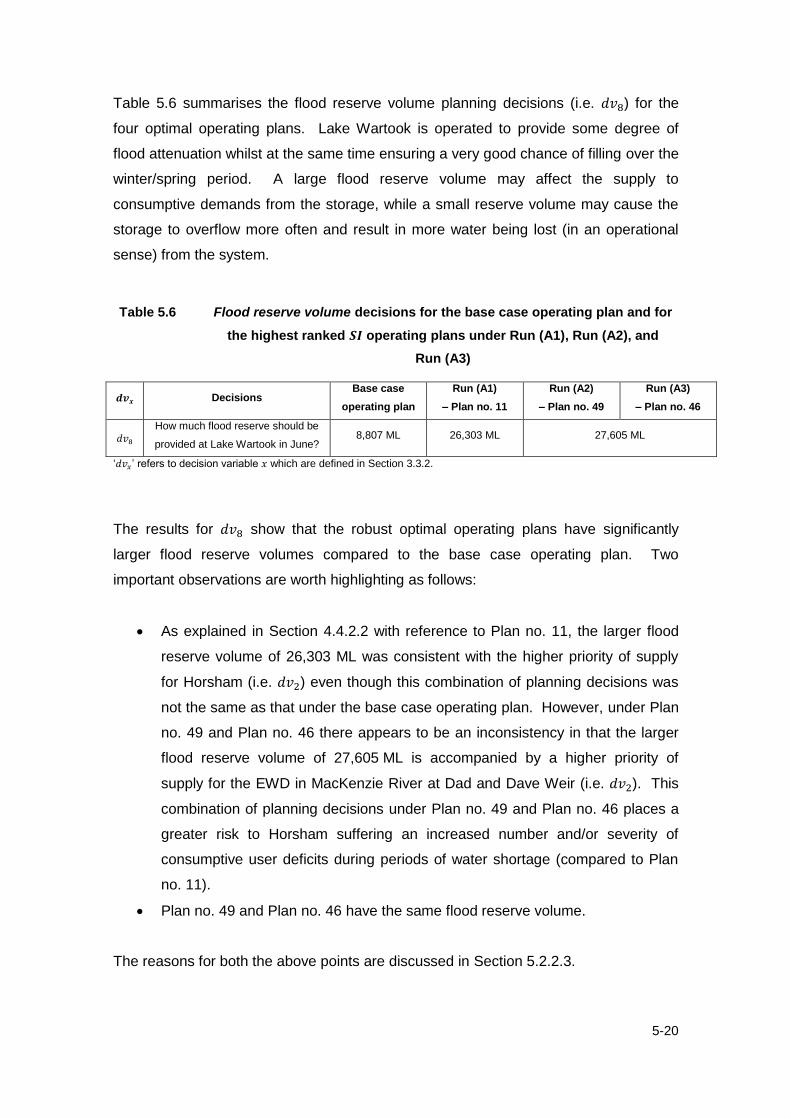
5-20
Table 5.6 summarises the flood reserve volume planning decisions (i.e. ) for the
four optimal operating plans. Lake Wartook is operated to provide some degree of
flood attenuation whilst at the same time ensuring a very good chance of filling over the
winter/spring period. A large flood reserve volume may affect the supply to
consumptive demands from the storage, while a small reserve volume may cause the
storage to overflow more often and result in more water being lost (in an operational
sense) from the system.
Table 5.6 Flood reserve volume decisions for the base case operating plan and for
the highest ranked operating plans under Run (A1), Run (A2), and
Run (A3)
Decisions Base case
operating plan
Run (A1)
– Plan no. 11
Run (A2)
– Plan no. 49
Run (A3)
– Plan no. 46
How much flood reserve should be
provided at Lake Wartook in June? 8,807 ML 26,303 ML 27,605 ML
‘ ’ refers to decision variable which are defined in Section 3.3.2.
The results for show that the robust optimal operating plans have significantly
larger flood reserve volumes compared to the base case operating plan. Two
important observations are worth highlighting as follows:
As explained in Section 4.4.2.2 with reference to Plan no. 11, the larger flood
reserve volume of 26,303 ML was consistent with the higher priority of supply
for Horsham (i.e. ) even though this combination of planning decisions was
not the same as that under the base case operating plan. However, under Plan
no. 49 and Plan no. 46 there appears to be an inconsistency in that the larger
flood reserve volume of 27,605 ML is accompanied by a higher priority of
supply for the EWD in MacKenzie River at Dad and Dave Weir (i.e. ). This
combination of planning decisions under Plan no. 49 and Plan no. 46 places a
greater risk to Horsham suffering an increased number and/or severity of
consumptive user deficits during periods of water shortage (compared to Plan
no. 11).
Plan no. 49 and Plan no. 46 have the same flood reserve volume.
The reasons for both the above points are discussed in Section 5.2.2.3.

5-21
Table 5.7 compares the results for the planning decisions regarding the shares of
environmental allocation in the WGWSS (i.e. to ). As explained in Section
4.4.2.2, the annual environmental allocation of 40,560 ML is released at four locations
within the headworks, namely; the Glenelg River at Rocklands Reservoir (i.e. ),
MacKenzie River at Lake Wartook (i.e. ), Mt William Creek at Lake Lonsdale (i.e.
), and the Wimmera River at Taylors Lake.
Table 5.7 Share of environmental allocation decisions for the base case operating
plan and for the highest ranked operating plans under Run (A1),
Run (A2), and Run (A3)
Decisions Base case
operating plan
Run (A1)
– Plan no. 11
Run (A2)
– Plan no. 49
Run (A3)
– Plan no. 46
How much of the
environmental water
allocation should be
released in the Glenelg
River basin?
Up to 40% of the
environmental
water allocation
Up to 15% of the
environmental
water allocation
Up to 8% of the environmental water
allocation
How much of the
environmental water
allocation should be
released in the Wimmera
basin at Lake Wartook?
Up to 30% of the
remaining share of
the environmental
water allocation
after that provided
for the Glenelg
basin
Up to 2% of the
remaining share of
the environmental
water allocation
after that provided
for the Glenelg
basin
Up to 22% of the remaining share of the
environmental water allocation after that
provided for the Glenelg basin
How much of the
environmental water
allocation should be
released in the Wimmera
basin at Lake Lonsdale?
Up to 60% of the
remaining share of
the environmental
water allocation
after that provided
for the Glenelg
basin and that at
Lake Wartook
Up to 2% of the
remaining share of
the environmental
water allocation
after that provided
for the Glenelg
basin and that at
Lake Wartook
Up to 19% of the remaining share of the
environmental water allocation after that
provided for the Glenelg basin and that at
Lake Wartook
‘ ’ refers to decision variable which are defined in Section 3.3.2.
Note that the Taylors Lake environmental allocation share is not included in Table 5.7,
as it is by default the remaining share of the environmental allocation after that
provided at Rocklands Reservoir, Lake Wartook, and Lake Lonsdale. The results for
to show that the environmental allocation shares under the robust optimal
operating plans represent a significant change from the base case operating plan. For
instance in terms of the Glenelg basin shares ( ), there is a major shift of
environmental allocation from the Glenelg basin to the Wimmera basin (i.e. 40% under

5-22
the base case operating plan to 8% under Plan no. 49 and Plan no. 46). The results
for and also show that the robust optimal operating plans have markedly
different shares at Lake Wartook and Lake Lonsdale respectively. Interestingly, the
results for the environmental allocation shares show a similar pattern to that observed
in the flood reserve volume planning decisions (i.e. ), in terms of the way Plan no.
11 differs from the planning decisions made under Plan no. 49 and Plan no. 46:
As explained in Section 4.4.2.2 with reference to Plan no. 11, the larger flood
reserve volume of 26,303 ML was consistent with the smaller environmental
allocation share at Lake Wartook (i.e. ) even though this combination of
planning decisions was not the same as that under the base case operating
plan. The consistency occurred given that the larger flood reserve volume
would increase the volume of water released to the MacKenzie River and Burnt
Creek downstream and provide more water for EWDs than that under the base
case operating plan. This would have the effect of reducing the environmental
allocation share at Lake Wartook under Plan no. 11 compared to that under the
base case operating plan. However, under Plan no. 49 and Plan no. 46 there
appears to be an inconsistency in that the larger flood reserve volume of
27,605 ML is accompanied by a large environmental allocation share at Lake
Wartook (i.e. ). This combination of planning decisions under Plan no. 49
and Plan no. 46 places a greater risk to Horsham in addition to that which would
already occur given the higher priority of supply for the EWD in MacKenzie
River at Dad and Dave Weir (i.e. ) as mentioned earlier.
Plan no. 49 and Plan no. 46 have the same environmental allocation shares at
all four sites.
In contrast to the above observations, there appears to be consistency among the
robust optimal operating plans with respect to holding water in Lake Lonsdale for
supply to consumptive demands (i.e. ) together with the increased environmental
allocation share at Taylors Lake compared to the base case operating plan. It is noted
however that unlike that under Plan no. 11 which has a negligible share at Lake
Lonsdale (i.e. ), the results for Plan no. 49 and Plan no. 46 show that the storage
would continue to play a role in supplying EWDs similar to that under the base case
operating plan, albeit with a smaller environmental allocation share.

5-23
Table 5.8 compares the results for the flow path planning decisions (i.e. and ).
Decision variable provides a flow path for resources in the eastern parts of the
WGWSS to supply EWDs in the Wimmera River and consumptive demands via the
Wimmera Mallee Pipeline. These resources include catchment flows intercepted by
Fyans Creek and Mt William Creek and water held in Lake Bellfield, Lake Fyans and
Lake Lonsdale. Decision variable relates to the maintenance of water quality in
terms of the mixing of water sourced from Lake Bellfield with that sourced from the
Wimmera River via Taylors Lake.
Table 5.8 Flow path decisions for the base case operating plan and for the highest
ranked operating plans under Run (A1), Run (A2), and Run (A3)
Decisions Base case
operating plan
Run (A1)
– Plan no. 11
Run (A2)
– Plan no. 49
Run (A3)
– Plan no. 46
Should Mt William Creek flows be
harvested into Wimmera Inlet
Channel or should all these flows
be passed down to Wimmera
River?
Harvesting of flows into Wimmera Inlet Channel is allowed
Should water from Lake Bellfield
be mixed with water from Taylors
Lake via the Bellfield-Taylors
Pipeline?
Yes, in a
proportion based
on the volume in
Lake Bellfield
No mixing via the Bellfield-Taylors Pipeline*
‘ ’ refers to decision variable which are defined in Section 3.3.2. * Mixing of water from Lake Bellfield and Taylors Lake can still occur provided that allows for harvesting of flows into Wimmera Inlet Channel.
The results for show that the base case operating plan and the robust optimal
operating plans harvest Mt William Creek flows into the Wimmera Inlet Channel.
However, in the case of the results show a significant change in terms of the flow
path used to transfer water from Lake Bellfield to Taylors Lake. Whilst this differs from
the manner in which the two storages operate, this decision is consistent with holding
water in Lake Lonsdale for supply to meet consumptive demands via the Wimmera
Mallee Pipeline (i.e. ). In essence, this would mean that Lake Bellfield would make
more water transfers to Lake Lonsdale for consumptive supply purposes rather than
using the Bellfield-Taylors Pipeline (as is currently the case shown under the base case
operating plan). The implications of such changes were discussed in Section 4.4.2.3.
Again, as observed in the flood reserve volume at Lake Wartook (i.e. ) and in the
environmental allocation shares (i.e. to ) under Plan no. 49 and Plan no. 46,

5-24
the O-S model adopted the same decision variable values for and . The
reason for the O-S model adopting the same values under both runs is explained in
Section 5.2.2.3.
Table 5.9 and Table 5.10 summarise the planning decisions relating to storage
maximum operating volumes (i.e. to ) and storage drawdown priorities and
storage targets (i.e. to ) respectively. Interestingly, identical results occur
under Plan no. 49 and Plan no. 46 for to . Note that with respect to all
planning decisions, this pattern occurs for consecutive decision variables from to
. The reason for the O-S model adopting the same values under both runs is
explained in Section 5.2.2.3. It is also worth highlighting that Taylors Lake is the only
storage that has higher storage maximum operating volumes under Plan no. 11, Plan
no. 49, and Plan no. 46 compared to the base case operating plan. This is indicative of
increased harvesting of unregulated flow from the Wimmera River at Taylors Lake to
compensate for the decreased harvesting at the other storages (by virtue of their lower
storage maximum operating volumes).
Table 5.9 Storage maximum operating volume (MOV) decisions for the base case
operating plan and for the highest ranked operating plans under
Run (A1), Run (A2), and Run (A3)
Decisions Base case
operating plan
Run (A1)
– Plan no. 11
Run (A2)
– Plan no. 49
Run (A3)
– Plan no. 46
Toolondo Reservoir MOV 92,430 ML 46,215 ML 36,972 ML
Lake Lonsdale MOV Inlet is closed Inlet is open
Lake Bellfield MOV 76,000 ML 30,400 ML 45,600 ML
Taylors Lake MOV 26,960 ML 30,330 ML 26,960 ML
Rocklands Reservoir MOV 261,000 ML 208,800 ML 243,600 ML
Lake Lonsdale MOV 53,300 ML 52,000 ML 32,500 ML
Moora Moora Reservoir MOV 6,300 ML 2,520 ML 4,410 ML
Total storage maximum operating volume 515,990 ML 370,265 ML 390,042 ML
‘ ’ refers to decision variable which are defined in Section 3.3.2.

5-25
Table 5.10 Storage draw down priority and storage target decisions for the base case
operating plan and for the highest ranked operating plans under
Run (A1), Run (A2), and Run (A3)
Decisions
Base case
operating
plan
Run (A1)
– Plan no. 11
Run (A2)
– Plan no. 49
Run (A3)
– Plan no. 46
What should
be the
drawdown
priority of
the
headworks
storages?
Lake Wartook 2nd
6th 5
th
Moora Moora Reservoir 1st 4
th 1
st
Horsham storages 3rd 2
nd 3
rd
Rocklands Reservoir 8th 8
th 7
th
Toolondo Reservoir 4th 7
th 2
nd
Lake Bellfield 6th 3
rd 4
th
Lake Fyans 7th 5
th 6
th
Taylors Lake 5th 1
st 8
th
What should
be the
second point
on the target
curve for the
headworks
storages?
Lake Wartook 10,000 ML 8,790 ML 26,370 ML
Moora Moora Reservoir 2,000 ML 5,040 ML 5,670 ML
Horsham storages 328 ML 66 ML 197 ML
Rocklands Reservoir 69,540 ML 174,000 ML 313,200 ML
Toolondo Reservoir 5,000 ML 9,243 ML 18,486 ML
Lake Bellfield 10,000 ML 23,568 ML 31,424 ML
Lake Fyans 2,500 ML 9,230 ML 1,846 ML
Taylors Lake 8,500 ML 5,420 ML 21,680 ML
Total volume for second point on target curve 107,868 ML 235,357 ML 418,873 ML
What should
be the third
point on the
target curve
for the
headworks
storages?
Lake Wartook 29,300 ML 27,249 ML 27,835 ML
Moora Moora Reservoir 6,300 ML 5,922 ML 5,922 ML
Horsham storages 328 ML 249 ML 302 ML
Rocklands Reservoir 115,900 ML 330,600 ML 327,120 ML
Toolondo Reservoir 46,250 ML 50,837 ML 77,641 ML
Lake Bellfield 20,000 ML 51,064 ML 45,565 ML
Lake Fyans 10,000 ML 16,614 ML 16,799 ML
Taylors Lake 8,500 ML 11,924 ML 23,306 ML
Total volume for third point on target curve 236,578 ML 494,459 ML 524,489 ML
What should
be the fourth
point on the
target curve
for the
headworks
storages?
Lake Wartook 29,300 ML 28,685 ML 28,275 ML
Moora Moora Reservoir 6,300 ML 6,187 ML 5,998 ML
Horsham storages 328 ML 257 ML 320 ML
Rocklands Reservoir 260,775 ML 334,080 ML 333,384 ML
Toolondo Reservoir 46,250 ML 84,111 ML 80,599 ML
Lake Bellfield 78,560 ML 75,810 ML 55,463 ML
Lake Fyans 10,000 ML 18,091 ML 17,463 ML
Taylors Lake 8,500 ML 25,582 ML 24,444 ML
Total volume for fourth point on target curve 440,013 ML 572,803 ML 545,946 ML
‘ ’ refers to decision variable which are defined in Section 3.3.2.

5-26
The results in Table 5.9 and Table 5.10 show that there is consistency amongst the
robust optimal operating plans in that compared to the base case operating plan these
plans have lower total storage maximum operating volumes and higher storage target
volumes. Whilst the results for the storage drawdown priorities cannot be structured in
the same way as the storage maximum operating volumes and storage targets, the
results show that the priorities under the robust optimal operating plans would be
different from those under the base case operating plan.
Whilst there is consistency between these planning decisions (i.e. storage maximum
operating volumes, storage drawdown priorities, and storage targets) and other
relevant planning decisions under Plan no. 11 (as explained in Section 4.4.2.2), the
same is not apparent from the decisions under Plan no. 49 and Plan no. 46. For
example in the case of Rocklands Reservoir:
It was explained that the decrease in the storage maximum operating volume at
Rocklands Reservoir (i.e. ) from 261,000 ML under the base case operating
plan to 208,800 ML under Plan no. 11 had the effect of forcing water out of the
storage and so satisfying the downstream EWD at the risk of not satisfying the
consumptive demands (refer to consumptive users (6) to (9) in Figure 5.1).
This planning decision was consistent with placing higher priority in supplying
consumptive demands from Rocklands Reservoir over the EWD in the Glenelg
River under Plan no. 11 (i.e. ). However, under Plan no. 49 and Plan no. 46
the smaller reduction in the storage maximum operating volume at Rocklands
Reservoir from 261,000 ML under the base case operating plan to 243,600 ML
results in different priorities placed between supplying the consumptive
demands and EWD (i.e. ). The reason for the O-S model adopting the
different priorities of supply is explained in Section 5.2.2.3; and
It was explained that the increase in storage targets at Rocklands Reservoir for
the second point (i.e. from 69,540 ML under the base case operating plan to
174,000 ML under Plan no. 11, ), for the third point (i.e. from 115,900 ML
under the base case operating plan to 330,600 ML under Plan no. 11, ),
and the fourth point (i.e. from 260,775 ML under the base case operating plan
to 334,080 ML under Plan no. 11, ) had the effect of increasing the rate of
harvest at Rocklands Reservoir. Such planning decisions were required in
order to satisfy the EWD in the Glenelg River by compensating for the reduced

5-27
share of environmental allocation under Plan no. 11 (i.e. ). The same
pattern, albeit to a greater extent, occurs under Plan no. 49 and Plan no. 46,
particularly for the second point (i.e. from 69,540 ML under the base case
operating plan to 313,200 ML under Plan no. 49 and Plan no. 46, ).
In summary, the results for the robust optimal operating plans (i.e. to ) show
that 21 out of 24 planning decisions under Plan no. 11; 20 out of 24 planning decisions
under Plan no. 49; and 19 out of 24 planning decisions under Plan no. 46 are different
from those under the base case operating plan. Interestingly, all but one of the 24
planning decisions (i.e. ) are identical under Plan no. 49 and Plan no. 46. The
reason for the O-S model adopting different priorities of supply for the consumptive
demands from Rocklands Reservoir and the EWD in the Glenelg River is explained in
Section 5.2.2.3.
5.2.2.3 Discussion
The analysis of the base case operating plan and the highest ranked operating plans
under three hydro-climatic conditions in Sections 5.2.2.1 and 5.2.2.2 raised the
following points for further discussion:
The and results for Plan no. 49 and Plan no. 46 were identical under all
three hydro-climatic conditions (refer to Table 5.4). This was shown to be
consistent with both plans having the same decision variable values for all but
one of the 24 planning decisions (i.e. ). Note that decision variable
relates to the priority of supply between the consumptive demands from
Rocklands Reservoir and the EWD in the Glenelg River (downstream of the
storage). However, it was not apparent from the (objective space and decision
space) results presented as to the reason for this difference in other than
that the plans were found under two separate O-S model runs, each of which
assumed a different GHG emission scenario (i.e. Plan no. 49 was the highest
ranked operating plan found under low to medium GHG emissions and Plan
no. 46 was the highest ranked operating plan found under medium to high
GHG emissions).
The value for Plan no. 11, the highest ranked operating plan found by the
O-S model under historic hydro-climatic conditions, was higher than the
corresponding highest ranked operating plans that were found under both

5-28
GHG emission scenarios. It is important to highlight that the reason for this
occurrence is due to the limited number of generations which were used in the
O-S modelling procedure (i.e. 5 generations). Whilst it has not been confirmed
in this thesis, it is expected that with the use of parallel processing and higher
computational processing power, a greater number of modelling generations
would have found operating plans with values greater than their Plan no. 11
counterparts, under both GHG emission scenarios. Nevertheless a comparison
of Plan no. 49 and Plan no. 46 revealed that Plan no. 11 favoured social and
consumptive interests for water over environmental interests. Whilst the results
in the objective space did not provide any supporting information for this
occurrence, there appears to be some explanation provided by certain
differences in the decision variable values among the three robust optimal
operating plans (i.e. Plan no. 11, Plan no. 49, and Plan no. 46). For instance, it
was explained that the inconsistency in the planning decisions regarding the
operation of Lake Wartook (i.e. , and ) and Rocklands Reservoir
(i.e. and ) may adversely impact consumptive user demands and as a
consequence provide favourable conditions for EWDs under Plan no. 49 and
Plan no. 46. However, the results presented were not able to confirm whether it
was Lake Wartook or Rocklands Reservoir, or both storages that caused a
reduction in the social and consumptive interests for water over an
improvement in environmental interests under Plan no. 49 and Plan no. 46.
Both the above points highlight the importance of using simulation modelling in order to
emulate the behaviour of the system under the effect of unproven optimal operating
plans, particularly those plans which consider future GHG emission scenarios. This
simulation modelling output can be used to provide the DM with a more detailed
appreciation of the impacts (beyond that provided by the performance metrics alone)
without any risk to human life, ecological health, and the water resources of the
WGWSS. Table 5.11 is a summary of the simulation modelling outputs for the base
case operating plan and the highest ranked operating plans presented thus far in
terms of a water balance for the WGWSS. A water balance is a holistic summary of
the effects of the three hydro-climatic conditions on different parts of the WGWSS over
the entire planning period (i.e. the availability of surface water in the various streams
referred to as ‘inflow’ and also the water that leaves the system referred to as ‘outflow’).

5-29
Table 5.11 Water balance for operating plans under historic hydro-climatic conditions and two GHG emission scenarios – ML/year
* refers to operating plans that have been modelled under the given hydro-climatic conditions using simulation-only as distinct to plans that have been found by optimisation-simulation modelling 1. ‘Inflow’ refers storage inflows and overland or catchment flows intercepted by streams and open channels within the Wimmera-Glenelg Water Supply System 2. Inflow to Langi Ghiran, Mt Cole, and Panrock reservoirs 3. ‘Consumptive use’ refers to consumptive users (1) to (30) as shown in Figure 5.1. 4. The storages, open channels and pipelines that are used to transfer water from Lake Bellfield to Lake Fyans and to Lake Lonsdale, and from Lake Fyans to Lake Lonsdale 5. The storages, open channels and pipelines that are used to transfer water from Moora Moora Reservoir to environmental water demands (3), and from Lake Wartook to Horsham Reservoir and
to environmental water demands (2) to (4) 6. The storages, open channels and pipelines that are used to transfer water from Rocklands Reservoir to Toolondo Reservoir and to Taylors Lake 7. ‘Environmental flow (regulated)’ refers to water that is released from storage to meet environmental water demands or EWDs (1) to (6) as shown in Figure 5.1. 8. ‘Environmental flow (unregulated)’ refers to run-of-river flows that contribute to environmental water demands or EWDs (1) to (6) as shown in Figure 5.1 including spills at Wannon River
diversion and minor storage spills at Langi Ghiran, Mt Cole, and Panrock reservoirs
Base case
operating
plan*
Run (A1)
- Plan no. 11Plan no. 49* Plan no. 46*
Base case
operating
plan*
Plan no. 11*Run (A2)
- Plan no. 49Plan no. 46*
Base case
operating
plan*
Plan no. 11* Plan no. 49*Run (A3)
- Plan no. 46
Inflow1: Glenelg River 102,552 102,552 102,552 102,552 92,028 92,028 92,028 92,028 91,284 91,284 91,284 91,284
Wannon River 15,936 15,936 15,936 15,936 11,004 11,004 11,004 11,004 9,780 9,780 9,780 9,780
Total Glenelg basin: 118,488 118,488 118,488 118,488 103,032 103,032 103,032 103,032 101,064 101,064 101,064 101,064
Wimmera River 98,412 98,412 98,412 98,412 86,184 86,184 86,184 86,184 81,492 81,492 81,492 81,492
Mt William Creek 73,200 73,200 73,200 73,200 72,504 72,504 72,504 72,504 68,100 68,100 68,100 68,100
Fyans Creek 28,740 28,740 28,740 28,740 23,592 23,592 23,592 23,592 21,972 21,972 21,972 21,972
McKenzie River and Burnt Creek 37,668 37,668 37,668 37,668 30,648 30,648 30,648 30,648 27,924 27,924 27,924 27,924
other minor streams2 4,764 4,764 4,764 4,764 3,588 3,588 3,588 3,588 3,684 3,684 3,684 3,684
Total Wimmera basin: 242,784 242,784 242,784 242,784 216,516 216,516 216,516 216,516 203,172 203,172 203,172 203,172
Total inflow: 361,272 361,272 361,272 361,272 319,548 319,548 319,548 319,548 304,236 304,236 304,236 304,236
Consumptive use3: Users (1) to (5) 6,672 6,503 6,442 6,442 6,528 6,360 6,216 6,216 5,784 5,844 5,592 5,592
Users (6) to (9) 6,314 6,734 6,470 6,470 6,804 6,792 6,648 6,648 6,785 6,817 6,673 6,673
Users (10) to (18) 4,176 4,212 4,200 4,200 4,176 4,164 4,140 4,140 4,164 4,176 4,152 4,152
Users (19) to (30) 33,312 33,640 32,560 32,560 34,308 34,464 33,984 33,984 34,104 34,343 33,924 33,924
Total consumptive use: 50,474 51,089 49,672 49,672 51,816 51,780 50,988 50,988 50,837 51,180 50,341 50,341
Headworks loss: Eastern section4 22,556 32,639 28,223 28,223 26,404 39,961 33,400 33,400 23,939 36,949 30,017 30,017
Central section5 10,948 9,086 10,532 10,532 10,592 9,920 10,111 10,111 9,786 9,038 9,395 9,395
Western section6 28,433 27,607 30,167 30,167 37,560 46,537 48,400 48,400 38,834 45,406 47,897 47,897
Total headworks loss: 61,937 69,332 68,922 68,922 74,556 96,419 91,910 91,910 72,559 91,393 87,308 87,308
Environmental flow (regulated)7: EWD (1) 6,619 3,451 2,395 2,395 11,977 5,371 3,140 3,140 13,078 5,626 3,182 3,182
EWDs (2) to (4) - - - - - - - - - - - -
EWDs (5) and (6) 6,205 569 3,284 3,284 12,070 738 5,545 5,545 10,732 733 5,573 5,573
Total environmental flow (regulated): 12,824 4,020 5,680 5,680 24,047 6,109 8,686 8,686 23,809 6,359 8,755 8,755
Environmental flow (unregulated)8: EWD (1) 56,562 60,575 51,234 51,234 33,725 30,858 25,681 25,681 31,406 32,045 27,329 27,329
EWDs (2) to (4) 23,874 19,903 20,809 20,809 17,293 14,324 15,869 15,869 15,955 13,532 14,548 14,548
EWDs (5) and (6) 141,687 144,437 153,255 153,255 109,198 111,638 118,169 118,169 101,759 102,400 108,666 108,666
Wannon River 12,526 10,270 10,271 10,271 7,777 6,781 6,781 6,781 7,050 6,031 6,031 6,031
other minor streams 3,688 3,817 3,534 3,534 2,628 2,734 2,561 2,561 2,767 2,858 2,731 2,731
Total environmental flow (unregulated): 238,336 239,002 239,103 239,103 170,622 166,335 169,061 169,061 158,937 156,867 159,305 159,305
Change in storage: 2,300- 2,171- 2,104- 2,104- 1,492- 1,095- 1,097- 1,097- 1,907- 1,563- 1,474- 1,474-
Total outflow: 361,272 361,272 361,272 361,272 319,548 319,548 319,548 319,548 304,236 304,236 304,236 304,236
Historic hydro-climatic conditions Low to medium GHG emissions Medium to high GHG emissions
Inflows and outflows of the Wimmera-Glenelg Water Supply System
(Note: Total inflow equals total outflow)

5-30
For instance, compared to the historic hydro-climatic conditions the results show that
there is a 12% reduction in the availability of water under the low to medium GHG
emission scenario (i.e.
) and a 16% reduction under the medium to high
GHG emission scenario (i.e.
). Moreover, the results show that the
reduction is varied among the streams compared to historic hydro-climatic conditions.
Using this same approach, the Glenelg basin would experience reductions of 13% and
15% under low to medium and medium to high GHG emissions respectively. In
contrast, the Wimmera basin would experience reductions of 11% and 16% under low
to medium and medium to high GHG emissions respectively.
The effect of the three hydro-climatic conditions is also shown in terms of the outflows
from the WGWSS. Table 5.11 provides a breakdown of the various consumptive users
and environmental water demands (EWDs) as shown in Figure 5.1, and headworks
loss in terms of the storage evaporation and transmission losses that would occur in
the eastern, central, and western parts of the WGWSS. Compared to the average of
the total consumptive use across the four operating plans under the historic hydro-
climatic conditions (i.e.
), the results show that the
average annual consumptive use volume increases by 2% (i.e.
) and 1% (i.e.
) under low to
medium and medium to high GHG emissions respectively. Using this same approach,
the average of the total headworks loss across the four operating plans increases by
32% and 26% under low to medium and medium to high GHG emissions respectively.
Interestingly, the base case operating plan has the lowest total headworks loss
compared to the other plans under each of the three hydro-climatic conditions.
In terms of the releases from storage to the EWDs, the results show that the average of
the total environmental flow (regulated) across the four operating plans increases by
69% under the two GHG emission scenarios and that this is largely attributed to the
base case operating plan. In fact, the results show that compared to the base case
operating plan, the other plans would cause a significant reduction in the total
environmental flow (regulated) compared to a small change in the total consumptive
use under each of the three hydro-climatic conditions. The implications of this
disproportionate impact between consumptive users and the regulated environmental
flows are discussed later in Section 5.2.2.3. It is also worth highlighting that compared
5-31
to the base case operating plan, the change in total environmental flows (regulated)
and the change in total consumptive use differs for Plan no. 11 and both Plan no. 49
and Plan no. 46. The results show that under all three hydro-climatic conditions, Plan
no. 11 supplies more water on average to consumptive use and less water to regulated
environmental flows compared to Plan no. 49 and Plan no. 46. These changes in the
regulated environmental flows and consumptive use volumes are discussed later in
Section 5.2.2.3. Whilst the results show an increase in the average of the total
environmental flow (regulated) across the four operating plans, the run-of-river in the
WGWSS would experience a significant decline under the GHG emissions scenarios.
Compared to the average of the total environmental flows (unregulated) across the four
operating plans under the historic hydro-climatic conditions, the results show that there
would be a decrease of 29% and 34% under low to medium and medium to high GHG
emissions respectively.
It is important to highlight that the level of aggregation of the various inflows and
outflows of the water balance has been tailored for the purposes of providing a direct
response to the two points of discussion mentioned earlier in Section 5.2.2.3. Thus,
the O-S modelling results (i.e. Sections 5.2.2.1 and 5.2.2.2) together with the
supporting information provided by the simulation modelling outputs (i.e. Table 5.11),
provide the following explanation for these two points of discussion:
The first point of discussion was in relation to the different values under
Plan no. 49 and Plan no. 46 representing the priority of supply between the
consumptive demands from Rocklands Reservoir and the EWD in the Glenelg
River (refer to consumptive users (6) to (9) and EWD (1) in Figure 5.1). As
explained in Section 3.2.3.2, in addition to Rocklands Reservoir serving as an
important source of water to consumptive users (6) to (9) and EWD (1) it also
supports the entire WGWSS by holding the majority of carryover water, reserve
for following year, and water to users in the Wimmera basin either through
direct supplies or by substitution with local sources of supply (i.e. consumptive
users (1) to (5) and (10) to (30)). This means that is influenced by the
availability of water in both the Glenelg River and Wimmera basin. The results
in Table 5.11 show that the decline in the availability of water in the Glenelg
River relative to historic hydro-climatic conditions is 10% (i.e.
) and
11% (i.e.
) compared to a decline in the Wimmera basin of 11%

5-32
(i.e.
) and 16% (i.e.
) under low to medium and medium
to high GHG emissions respectively. On this basis, it would appear that the
larger reduction in the Wimmera basin under medium to high GHG emissions
(i.e. 16%) is consistent with adopting a higher priority for the EWD in the
Glenelg River in order to ensure that environmental flows are provided water
first before consumptive users under Plan no. 46. Despite this reasoning, the
simulation modelling results for Plan no. 49 under medium to high GHG
emissions confirm that is not sensitive to the decline in water availability
(caused by the GHG emissions) given that the results are the same as the O-S
modelling results for Plan no. 46 under the same GHG emission scenario. Note
that the same effect is observed in the simulation modelling results for Plan no.
46 under low to medium GHG emissions compared to the O-S modelling results
for Plan no. 49 under the same GHG emission scenario.
The second point of discussion was in relation to the way in which the impacts
of the GHG emissions were shared amongst the four interests for water (i.e.
environmental, social, consumptive, and system-wide interests). Compared to
Plan no. 49 and Plan no. 46, the results showed that Plan no. 11 favoured
social and consumptive interests for water over environmental interests (refer to
Table 5.4). The average annual volumes for consumptive users (1) to (30)
under Plan no. 11 are consistently higher than those under Plan no. 49 and
Plan no. 46 for all three hydro-climatic conditions (refer to Table 5.11). This
confirms that the higher consumptive use volumes under Plan no. 11 would
occur across the whole WGWSS and not be localised solely around Lake
Wartook and Rocklands Reservoir as the planning decision results indicated in
Section 5.2.2.2. Moreover, the average annual headworks loss volumes in the
eastern section (which are largely attributed to Lake Lonsdale) are consistently
higher under Plan no. 11 indicating that the eastern storages would be holding
more water than that under Plan no. 49 and Plan no. 46. Note that this is
confirmed by the better performing objective functions for Lake Lonsdale (i.e.
higher and values and the lower value) under Plan no. 11 compared to
those under Plan no. 49 and Plan no. 46 under the GHG emission scenarios
(refer to Table 5.4).
It is worth noting that in Victoria (Australia) a decline in the long-term availability of
water which has a disproportionate effect on the environment or on consumptive use

5-33
may trigger a review of the long-term water resources to determine the actions required
to restore the balance between the environment and consumptive use (Section 22P of
the Water Act 1989 (Vic)). In the context of the disproportionate impact between
consumptive users and environmental flows discussed earlier, it would be prudent to
explicitly account for such disproportionality in the formulation of higher order MOOPs
in order to guide the optimisation search towards more equitable solutions.
Moreover, the water balance results for the base case operating plan raise another
important point in regards to the formulation of the MOOPs presented. In comparison
to the robust optimal operating plans, the results in Table 5.11 suggest that the base
case operating plan is a viable alternative plan in terms of it consistently providing (i)
similar consumptive use volumes; (ii) the lowest volumes of headworks loss; and (iii)
the highest total (regulated and unregulated) environmental flow volumes under the
three hydro-climatic conditions. This highlights the importance of properly formulating
the MOOP to represent all interests for water including operational efficiency which
could have been expressed as a system-wide interest for water in substitution for (or
addition to) users’ water allocations. The corresponding objective function would have
minimised the volume of headworks loss and potentially have guided the optimisation
search towards more efficient modes of operation; thus finding optimal operating plans
that dominated the base case operating plan.
It is important at this point to refer to a recent review of the operation of the WGWSS
(using a REALM simulation modelling approach) which showed that the base case
operating plan was generally consistent with stakeholders’ storage management
objectives (GWMWater, 2014). This review made 40 recommendations to improve
system operation which are summarised below. Note that the management objectives
are in italics font and the number in brackets refers to the number of recommendations
made with respect to that particular management objective:
“To direct operations to ensure that the structural and operational integrity of the
Wimmera-Mallee system headworks is maintained.”
Improve overall system efficiency by introducing a range of works (x2)
“To deliver water to entitlement holders in a timely, transparent and efficient
manner.”
Formalising existing arrangements in the delivery of environmental flows (x1)

5-34
“To account for the water stored and water flows in the Wimmera-Mallee
system
headworks and for the water taken by entitlement holders.”
Improving water accounting particularly for carryover (x6)
“To maintain and, when the need arises, to enhance, the security of supply to
water entitlement holders with particular emphasis on contingency planning to
avoid water shortages and measures to reduce water losses in the Wimmera-
Mallee system headworks.”
Improving flexibility in water delivery by increasing the maximum operating
volume from 75% to 85% full supply volume for Rocklands Reservoir (x6)
“To facilitate the transfer of water entitlements and allocations between
entitlement holders.”
Educating water users of the benefits of water trade through the preparation of
guidance papers (x1)
“To facilitate the implementation of environmental watering activities, including
activities under the environmental operating plan.”
Developing more holistic management plans that improve watering
arrangements between water agencies (x6)
“To facilitate the achievement of environmental outcomes, and mitigate
significant environmental events, such as fish kills, unseasonal water, algal
blooms, river bank erosion and acidification.”
Developing a collaborative approach to addressing water quality issues (x2)
“To manage water quality in the Wimmera-Mallee system headworks so that it
is fit for purpose for urban, irrigation, industrial, stock and domestic, and
environmental use.”
Improving water quality monitoring by expanding current arrangements to
include other parts of the system (x1)
“To provide opportunities for recreation activities in the Wimmera-Mallee system
headworks where that is compatible with other objectives.”
Improving the recreation amenity at sites in the system that have high social
value by employing a range of works including increasing the recreation water
entitlement (x10)
“To manage floods in the Wimmera-Mallee system headworks to conserve
water and manage impacts on communities, including the supply of water to
recreational lakes where this is compatible with the environmental objectives.”

5-35
Improving the guidelines for storage operations during floods (x3)
“To facilitate the protection of Aboriginal cultural heritage, in accordance with
relevant cultural heritage management plans and by other means.”
Improving involvement of indigenous groups in planning processes (x1)
(Development of an implementation plan, which was not a specific management
objective, was also recommended as part of the review project in order to assist
with the delivery of the above recommendations, x2)
Based on the number of recommendations under each management objective, the
social interests for water in terms of recreation amenity was one area that required a
great deal of attention (i.e. 10 out of 40 recommendations). Another two areas
requiring a higher level of attention which are particularly relevant to this study are the
recommendations to develop more holistic management plans for improving
environmental watering arrangements and the recommendations to increase the
maximum operating volume at Rocklands Reservoir. The first and second of these
recommendations, are directly related to the problem formulation phase which ought to
explicitly account for all interests for water. The third of these recommendations is in
contradiction to the results for the highest ranked operating plans found by the O-S
model under each of the three hydro-climatic conditions considered in this thesis (refer
to in Table 4.11). However as explained earlier, the formulation of the MOOPs
using system-wide interests in terms of users’ water allocations (instead of headworks
loss) may not necessarily be able to guide the optimisation search towards more
efficient modes of operation.
5.2.3 Conclusions
The purpose of Section 5.2 was to confirm the validity of the optimal operating plans
found under historic hydro-climatic conditions in Chapter 4 (i.e. Run (A1)) against the
optimal operating plans under the low to medium level GHG emission scenario (i.e.
Run (A2)) and the medium to high level GHG emission scenario (i.e. Run (A3)). The
outcomes of the analysis of the base case operating plan and the highest ranked
operating plans found by the O-S model under each of the three hydro-climatic
conditions are summarised as follows:

5-36
The curves of the optimal operating plans under Run (A1) and Run (A3)
showed that the base case operating plan was neither the highest nor the
lowest in terms of the level of sustainability that could be achieved in the
WGWSS (in terms of ). Note that the dominance test for the base case
operating plan against the optimal plans under Run (A2) confirmed that the
base case operating plan was not optimal under low to medium GHG
emissions. The highest ranked operating plans under Run (A1), Run (A2),
and Run (A3) were Plan no. 11 ( ), Plan no. 49 ( ), and
Plan no. 46 ( ) respectively.
The dominance test and the were used to short list optimal operating plans
that were considered robust (i.e. capable of withstanding the changed hydro-
climatic conditions given by the GHG emissions under Run (A2) and Run (A3)).
The dominance test results together with the values showed that the highest
ranked operating plans were indeed robust whereas the base case operating
plan was not robust given that it was not optimal under low to medium GHG
emissions. However the simulation modelling outputs (in the form of a water
balance) showed that the base case operating plan consistently provided (i)
similar consumptive use volumes; (ii) the lowest volumes of headworks loss;
and (iii) the highest total (regulated and unregulated) environmental flow
volumes under the three hydro-climatic conditions.
In general, the results for Plan no. 49 under Run (A2) and Plan no. 46 under
Run (A3) showed a degree of inconsistency with the planning decisions for Plan
no. 11 under Run (A1). This inconsistency suggested that consumptive users
at Lake Wartook and/or Rocklands Reservoir would experience a greater
impact than that under historic hydro-climatic conditions. These results
together with the water balance results showed that (i) the apparent
inconsistency was in fact an alternative set of optimal operating rules (to those
under Plan no. 11) which favoured environmental interests for water over social
and consumptive interests; and (ii) that the impact would be experienced by all
consumptive users in the system and not localised around Lake Wartook and
Rocklands Reservoir.
The water balance results also showed that there would be a disproportionate
impact between environmental flows and consumptive users under the highest
ranked operating plans compared to that under the base case operating plan.
The results for the highest ranked operating plans showed that there would

5-37
be a significant reduction in the total environmental flow (regulated) compared
to a small change in the total consumptive use under each of the three hydro-
climatic conditions.
Plan no. 49 and Plan no. 46 had identical values which meant that their
values and values were identical under each of the three hydro-climatic
conditions. The outcomes of the decision space analysis showed that the
reason for the two plans achieving the same level of sustainability for the
WGWSS was due to these plans sharing the same value for all but one of the
decision variables. It was explained that the one exception was the planning
decision representing the priority of supply between the consumptive demands
from Rocklands Reservoir and the EWD in the Glenelg River (i.e. ), and that
its value was influenced by the availability of water in both the Glenelg River
and Wimmera basin. On balance, the results showed that was not sensitive
to the decline in water availability caused by the GHG emissions.
The outcomes of a recent review of the operation of the WGWSS showed that the base
case operating plan was generally consistent with stakeholders’ storage management
objectives. Of particular interest to this thesis was that the review made
recommendations to improve the inclusion of social interests for water in terms of
recreation amenity, to develop more holistic management plans for environmental
watering purposes, and to increase the maximum operating volume at Rocklands
Reservoir. The first and second of these recommendations are directly related to the
problem formulation phase which ought to explicitly account for all interests for water.
The third of these recommendations was in contradiction to the results for the highest
ranked operating plans found by the O-S model under each of the three hydro-
climatic conditions. However as explained earlier, the formulation of the MOOPs using
system-wide interests in terms of users’ water allocations (instead of headworks loss)
may not necessarily be able to guide the optimisation search towards more efficient
modes of operation. Moreover it was explained that the disproportionate impact borne
by the regulated environmental flows would be an important consideration in Victoria
(Australia) where such an in-balance could lead to a review of the management of
water resources.

5-38
5.3 Selection of preferred optimal operating plan for the WGWSS
According to Deb (2001) the ideal multi-objective optimisation approach involves
finding a diverse set of optimal solutions followed by the selection of a solution(s) using
higher-level qualitative information. The first of these two areas of work were described
in Chapter 3 to Chapter 5 (thus far). Chapter 3 presented a higher order MOOP for the
WGWSS which was structured hierarchically in terms of a value tree. The top of the
value tree represented the sustainability of the WGWSS corresponding to the for the
WGWSS. The bottom of the value tree consisted of various conflicting criteria which
corresponded to the 18 objective functions of the MOOP. Chapter 4 showed that this
problem formulation could be used by the O-S model to find the Pareto front of optimal
operating plans assuming historic hydro-climatic conditions. Section 5.2 tested the
validity of the base case operating plan and the highest ranked operating plan
(found under historic hydro-climatic conditions) assuming two plausible GHG emission
scenarios. This testing process allowed for the short-listing of three robust optimal
operating plans which were able to withstand all three hydro-climatic scenarios. The
second of the two areas of work described above is the subject of this section which
aims to incorporate stakeholders’ preferences in the D ’s selection of a preferred
optimal operating plan.
5.3.1 Stakeholder preferences
Having completed the problem formulation phase and found the Pareto fronts under all
three hydro-climatic conditions, it becomes necessary to develop a conceptual model
which represents stakeholders’ preferences and value judgements. Methods available
under the umbrella term multi-criteria decision analysis (MCDA) are widely used for the
purpose of facilitating the exploration of decisions that take explicit account of multiple
factors or criteria (Belton and Stewart, 2002). As explained in Chapter 3, the use of the
(in evaluating and comparing optimal operating plans) lends itself to the value
measurement preference model. This is due to the providing (i) a means of
associating a real number for each optimal operating plan; and (ii) an ordering or
ranking of these plans, where values of 0 and 1 represent the lowest and highest
levels of sustainability in the WGWSS respectively. The resulting th stakeholder’s
Weighted Sustainability Index, , is provided in Equation 5.10. Note that for ease of
referencing the relevant objective function equation in Chapter 5, is expressed in

5-39
terms of (i.e. the th stakeholder’s weight for the th objective function, ) instead of
(i.e. the th stakeholder’s weight for the th performance metric).
For the purposes of demonstrating the application of the , three sets of preference
vectors were gleaned from the available stakeholder information collected as part of
recent water resource planning studies of the WGWSS (GWMWater, 2007; 2012a;
2012b; DSE, 2011). These stakeholder preferences are assumed to represent those
stakeholders that have (i) higher environmental preferences relating to ecological
health of waterways including the flora and fauna that depend on these natural
ecosystems ; (ii) higher social preferences concerning water for recreation and
for maintenance of water quality ; and higher preferences for the needs of
consumptive users such as for urban centres, irrigators, and other water-dependant
industries . Figure 5.3 to Figure 5.5 are diagrammatic representations of the
value tree used in the formulation of the MOOP showing the preferences of the three
stakeholders (i.e. , , and ).
Note that for ease of presentation, the top of the tree is shown on the left of the figure
and the bottom of the tree (i.e. the leaves) are on the right. Accordingly, the Weighted
Sustainability Index representing environmental, social, and consumptive stakeholder
preferences are denoted ,
, and
respectively.

5-40
ote: ‘ ’ refers to objective function as defined in Section 5.2.1.
Figure 5.3 Value tree of a higher MOOP of WGWSS showing preferences of in
terms of cumulative weights (in italic font) and
corresponding ratios (in bold font)
It is important to distinguish between the two forms of stakeholder preferences
presented in Figure 5.3 to Figure 5.5 being cumulative weights in italic font and ratios in
bold font. As the uses a ratio scale of preferences, the ratios are used for the
bottom level of the value tree in the first instance. Note that the ratios are only shown
for the bottom level of the value tree in Figure 5.3 to Figure 5.5 given that the will
be computed from the corresponding 18 objective function values later in Section 5.3.2.
The second step involved normalising these ratios to produce cumulative weights
which allowed for higher levels of the value tree to be determined. Note that the
cumulative weight of a parent criterion is the total of the cumulative weights of its
descendants.
[f5] Minimum water level at Lake Lonsdale 0.02 (2)
[f8] Minimum water level at Lake Fyans 0.03 (3)
[f11] Minimum water level at Rocklands Reservoir 0.02 (2)
[f2] Environmental flow deficits at 6 locations 0.15 (15)
[f17] Total water allocation 0.09 (9)
Minimum storage levels for recreation amenity
0.15
Minimum storage levels for maintenance of water quality
0.07
Sub-indicatorIndicatorComponent
[f14] Consumptive user deficits of 30 user groups 0.02 (2)
Index
Social interests for water0.22
We
igh
ted
Su
stai
nab
ility
Ind
ex,
SISH
a
Environmental interests for water
0.45
[f3] Environmental flow deficits at 6 locations 0.10 (10)
[f1] Environmental flow deficits at 6 locations 0.20 (20)
[f18] Total water allocation 0.09 (9)
[f16] Total water allocation 0.09 (9)
[f15] Consumptive user deficits of 30 user groups 0.02(2)
[f13] Consumptive user deficits of 30 user groups 0.02 (2)
[f12] Minimum water level at Rocklands Reservoir 0.02 (2)
[f10] Minimum water level at Rocklands Reservoir 0.03 (3)
[f4] Minimum water level at Lake Lonsdale 0.03 (3)
[f6] Minimum water level at Lake Lonsdale 0.01 (1)
[f7] Minimum water level at Lake Fyans 0.04 (4)
[f9] Minimum water level at Lake Fyans 0.02 (2)
Environmental flow deficits at 6 locations
0.45
Consumptive interests for water
0.06
Consumptive user deficits of 30 user groups
0.06
System-wide interests for water
0.27
Total water allocation
0.27

5-41
ote: ‘ ’ refers to objective function as defined in Section 5.2.1.
Figure 5.4 Value tree of a higher MOOP of WGWSS showing preferences of in
terms of cumulative weights (in italic font) and
corresponding ratios (in bold font)
Figure 5.3 shows that considers the preferences of environmental, social,
consumptive, and system-wide interests for water to be in the ratio of 45:22:6:27 (i.e.
(20+15+10):(3+2+1+4+3+2+3+2+2):(2+2+2):(9+9+9). Note that the highest preference
for is attributed to the environmental interests for water (i.e. objective functions
to ) which is consistent with the earlier assumption. Figure 5.4 shows that
considers the preferences of environmental, social, consumptive, and system-wide
interests for water to be in the ratio of 6:66:6:22. Figure 5.5 shows that has the
same preferences as except for the environmental interests for water and the
consumptive interests which are reversed (i.e. 6:22:45:27).
[f5] Minimum water level at Lake Lonsdale 0.07 (7)
[f8] Minimum water level at Lake Fyans 0.07 (7)
[f11] Minimum water level at Rocklands Reservoir 0.08 (8)
[f2] Environmental flow deficits at 6 locations 0.02 (2)
[f17] Total water allocation 0.07 (7)
Minimum storage levels for recreation amenity
0.42
Minimum storage levels for maintenance of water quality
0.24
Sub-indicatorIndicatorComponent
[f14] Consumptive user deficits of 30 user groups 0.02 (2)
Index
Social interests for water0.66
We
igh
ted
Su
stai
nab
ility
Ind
ex,
SISH
b
Environmental interests for water
0.06
[f3] Environmental flow deficits at 6 locations 0.02 (2)
[f1] Environmental flow deficits at 6 locations 0.02 (2)
[f18] Total water allocation 0.07 (7)
[f16] Total water allocation 0.08 (8)
[f15] Consumptive user deficits of 30 user groups 0.02 (2)
[f13] Consumptive user deficits of 30 user groups 0.02 (2)
[f12] Minimum water level at Rocklands Reservoir 0.07 (7)
[f10] Minimum water level at Rocklands Reservoir 0.09 (9)
[f4] Minimum water level at Lake Lonsdale 0.08 (8)
[f6] Minimum water level at Lake Lonsdale 0.06 (6)
[f7] Minimum water level at Lake Fyans 0.08 (8)
[f9] Minimum water level at Lake Fyans 0.06 (6)
Environmental flow deficits at 6 locations
0.06
Consumptive interests for water
0.06
Consumptive user deficits of 30 user groups
0.06
System-wide interests for water
0.22
Total water allocation
0.22

5-42
ote: ‘ ’ refers to objective function as defined in Section 5.2.1.
Figure 5.5 Value tree of a higher MOOP of WGWSS showing preferences of in
terms of cumulative weights (in italic font) and
corresponding ratios (in bold font)
5.3.2 Post-processing results and discussion
5.3.2.1 Objective space
This section uses the results from O-S modelling runs presented in Section 4.4 and
Section 5.2 to calculate and for the th stakeholder (i.e. , , and ) with
respect to the th interest for water (i.e. environmental, social, consumptive, and
system-wide interests). The mathematical formulae for are given in Equations 5.6
to 5.9 and the is given in Equation 5.10.
[f5] Minimum water level at Lake Lonsdale 0.02 (2)
[f8] Minimum water level at Lake Fyans 0.03 (3)
[f11] Minimum water level at Rocklands Reservoir 0.02 (2)
[f2] Environmental flow deficits at 6 locations 0.02 (2)
[f17] Total water allocation 0.09 (9)
Minimum storage levels for recreation amenity
0.15
Minimum storage levels for maintenance of water quality
0.07
Sub-indicatorIndicatorComponent
[f14] Consumptive user deficits of 30 user groups 0.15 (15)
Index
Social interests to water0.22
We
igh
ted
Su
stai
nab
ility
Ind
ex,
SISH
c
Environmental interests to water
0.06
[f3] Environmental flow deficits at 6 locations 0.02 (2)
[f1] Environmental flow deficits at 6 locations 0.02 (2)
[f18] Total water allocation 0.09 (9)
[f16] Total water allocation 0.09 (9)
[f15] Consumptive user deficits of 30 user groups 0.10(10)
[f13] Consumptive user deficits of 30 user groups 0.20 (20)
[f12] Minimum water level at Rocklands Reservoir 0.02 (2)
[f10] Minimum water level at Rocklands Reservoir 0.03 (3)
[f4] Minimum water level at Lake Lonsdale 0.03 (3)
[f6] Minimum water level at Lake Lonsdale 0.01 (1)
[f7] Minimum water level at Lake Fyans 0.04 (4)
[f9] Minimum water level at Lake Fyans 0.02 (2)
Environmental flow deficits at 6 locations
0.06
Consumptive interests to water
0.45
Consumptive user deficits of 30 user groups
0.45
System-wide interests to water
0.27
Total water allocation
0.27

5-43
Table 5.12 summarises the three sets of and values for the robust optimal
operating plans (i.e. Plan no. 11, Plan no. 49, and Plan no. 46) with respect to each of
, , and . The first two columns under each of the three hydro-climatic
scenarios present these values without applying the stakeholder preferences. Note
that these values are the same as those presented earlier in Table 5.4. The third and
fourth columns under each of the three hydro-climatic scenarios present the and
with stakeholder preferences , , and applied to them as specified in
Equations 5.6 to 5.10. Note that Plan no. 49 and Plan no. 46 are combined in a single
column in each case as the results in Section 5.2 showed that the WGWSS performed
exactly the same under the two operating plans. The shaded results in Table 5.12
represent the best outcome (i.e. the highest values) between corresponding (non-
weighted and weighted) and values. The shading of the best outcome in each
case is colour-coded to align with the same hydro-climatic conditions (i.e. light/dark
grey shade - historic hydro-climatic conditions, light/dark red shade - low to medium
level GHG emissions, and light/dark green shade – medium to high level GHG
emissions). Note that for consistency, the values which do not have the stakeholder
preferences applied to them are the same light-coloured shade used in Table 5.3 and
Table 5.4.
Table 5.12 shows that the relativity between Plan no. 11 and Plan no. 49/Plan no. 46 in
terms of any corresponding and values is the same under each of the three
hydro-climatic conditions, regardless of the stakeholder preference applied. For
example, under the low to medium hydro-climatic conditions, the value of Plan
no. 11 is less than Plan no. 49/Plan no. 46 (i.e. ) and the same occurs in the
(i.e. ). Note that whilst the and relativities are the same, their
absolute values can change subject to the stakeholder preferences and, depending on
the product of these changed values, may cause to change relative to . Using
the same example, the stakeholder preferences caused a change in the values for
,
, and
changing the relativity between the values for Plan no.
11 and Plan no. 49/Plan no. 46 compared to the corresponding values (i.e.
c.f. ). Note that this same effect occurs three times
and is circled in red. This also means that with the exception of these three instances,
the stakeholder preferences did not change the relativities between and .

5-44
Table 5.12 Values of Component-level Index and Sustainability Index (without and with stakeholder preferences) for the shortlisted
robust optimal operating plans under historic hydro-climatic conditions and two GHG emission scenarios
‘ ’ refers to the Component-level Index for the i
th interest for water as defined in Section 5.1. Refer to Equations 5.6 to 5.9 for the Weighted Component-level Index.
‘ ’ refers to the Sustainability Index for the Wimmera-Glenelg Water Supply System as defined in Equation 5.5. Refer to Equation 5.10 for the Weighted Sustainability Index. * refers to operating plans that have been modelled under the given hydro-climatic conditions using simulation-only as distinct to plans that have been found by optimisation-simulation modelling. ‘na’ means not applicable.
Run (A1)
- Plan no. 11
Plan no. 49*
&
Plan no. 46*
Run (A1)
- Plan no. 11
Plan no. 49*
&
Plan no. 46*
Plan no. 11*
Run (A2)
- Plan no. 49
&
Plan no. 46*
Plan no. 11*
Run (A2)
- Plan no. 49
&
Plan no. 46*
Plan no. 11*
Plan no. 49*
&
Run (A3)
- Plan no. 46
Plan no. 11*
Plan no. 49*
&
Run (A3)
- Plan no. 46
SH a
CI env Environmental Component-level Index - Equations (5.1) & (5.6) 45 0.52 0.61 0.47 0.58 0.28 0.32 0.22 0.27 0.22 0.32 0.17 0.26
CI socio Social Component-level Index - Equations (5.2) & (5.7) 22 0.43 0.48 0.50 0.55 0.92 0.83 0.94 0.86 0.64 0.56 0.69 0.61
CI cons Consumptive Component-level Index - Equations (5.3) & (5.8) 6 0.70 0.54 0.66 0.47 0.74 0.47 0.69 0.40 0.48 0.39 0.42 0.32
CI sys System-wide Component-level Index - Equations (5.4) & (5.9) 27 0.52 0.53 0.52 0.53 1.00 1.00 1.00 1.00 1.00 1.00 1.00 1.00
SI Sustainability Index - Equations (5.5) & (5.10) na 0.50 0.52 0.50 0.55 0.74 0.66 0.49 0.51 0.55 0.53 0.40 0.46
SH b
CI env Environmental Component-level Index - Equations (5.1) & (5.6) 6 0.52 0.61 0.45 0.56 0.28 0.32 0.20 0.25 0.22 0.32 0.15 0.24
CI socio Social Component-level Index - Equations (5.2) & (5.7) 66 0.43 0.48 0.43 0.48 0.92 0.83 0.93 0.84 0.64 0.56 0.63 0.55
CI cons Consumptive Component-level Index - Equations (5.3) & (5.8) 6 0.70 0.54 0.66 0.47 0.74 0.47 0.69 0.40 0.48 0.39 0.42 0.32
CI sys System-wide Component-level Index - Equations (5.4) & (5.9) 22 0.52 0.53 0.53 0.54 1.00 1.00 1.00 1.00 1.00 1.00 1.00 1.00
SI Sustainability Index - Equations (5.5) & (5.10) na 0.50 0.52 0.46 0.50 0.74 0.66 0.84 0.77 0.55 0.53 0.63 0.58
SH c
CI env Environmental Component-level Index - Equations (5.1) & (5.6) 6 0.52 0.61 0.45 0.56 0.28 0.32 0.20 0.25 0.22 0.32 0.15 0.24
CI socio Social Component-level Index - Equations (5.2) & (5.7) 22 0.43 0.48 0.50 0.55 0.92 0.83 0.94 0.86 0.64 0.56 0.69 0.61
CI cons Consumptive Component-level Index - Equations (5.3) & (5.8) 45 0.70 0.54 0.67 0.49 0.74 0.47 0.71 0.43 0.48 0.39 0.44 0.35
CI sys System-wide Component-level Index - Equations (5.4) & (5.9) 27 0.52 0.53 0.52 0.53 1.00 1.00 1.00 1.00 1.00 1.00 1.00 1.00
SI Sustainability Index - Equations (5.5) & (5.10) na 0.50 0.52 0.57 0.52 0.74 0.66 0.77 0.61 0.55 0.53 0.57 0.51
Medium to high GHG emissions
Environmental stakeholder preferences: Values without SH a Values with SH a Values without SH a Values with SH a Values without SH a Values with SH a
Component-level
Index (CI i ) and
Sustainability
Index (SI )
Description
CI i (italic font) and SI (bold italic font)
Ratio
preference
for the j th
stakeholder
(SH J )
Historic hydro-climatic conditions Low to medium GHG emissions
Values with SH b
Consumptive stakeholder preferences: Values without SH c Values with SH c Values without SH c Values with SH c Values without SH c Values with SH c
Social stakeholder preferences: Values without SH b Values with SH b Values without SH b Values with SH b Values without SH b

5-45
Overall the and results show that there is consensus that Plan no. 49/Plan no. 46
is the most preferred under historic hydro-climatic conditions and that Plan no. 11 is
most preferred under the GHG emission scenarios.
5.3.2.2 Decision space
Section 5.2.2.2 presented a detailed analysis of the decision variable values for each of
the 24 planning decisions under Plan no. 11, Plan no. 49 and Plan no. 46. The
analysis (alone) showed that there was a degree of inconsistency with the planning
decisions under Plan no. 49 and Plan no. 46 compared to those under Plan no. 11.
However with the aid of a system water balance (refer to Section 5.2.2.3), the apparent
inconsistency in Plan no. 49 and Plan no. 46 was shown to be an alternative set of
optimal operating rules to those under Plan no. 11 which simply favoured
environmental interests for water over social and consumptive interests. This explains
in part the results in Table 5.12, in so far as the change in the relativity between the
values for Plan no. 11 and Plan no. 49/Plan no. 46 compared to the corresponding
values. That is, a stakeholder who has high environmental preferences such as
will accentuate this preference in the value for optimal plans like Plan no. 49 and
Plan no. 46 which already favour environmental interests for water. Similarly, a
stakeholder who has high consumptive preferences such as will accentuate this
preference in the value for optimal plans like Plan no. 11 which already favour
consumptive interests for water. On this basis, the reason that the preferences for
do not change from one plan to another is that the environmental and consumptive
preferences are the same. This means that the higher social preferences of
(alone) are not enough to change the preference for one plan over another for this
stakeholder. However, what is not known from this analysis is the preference ratio
which causes this reversal in relativities of and values. The answer to this
question requires further investigation and discussion as provided in Section 5.3.2.3.
5.3.2.3 Discussion
The results of the objective space analysis (i.e. Section 5.3.2.1) showed how the
could be used to select a preferred optimal operating plan by incorporating stakeholder
preferences in the . However Belton and Stewart (2002) point out that the
determination of an overall value (in a value measurement preference model) should
not be viewed as the end of the analysis. The authors explain that the value (i.e. the

5-46
in this case) ought to be considered as another step in furthering the understanding
and promoting discussion about the problem. Indeed, the like the is by definition
an indicator of the level of sustainability that can be achieved in the WGWSS under a
given optimal operating plan. The DM needs to be aware that further exploration is
required in terms of the composition of the optimal operating plan (i.e. decision space)
and in terms of the performance of the WGWSS beyond that provided by the
performance metrics alone (i.e. simulation modelling). Similarly, exploration of
alternative perspectives of the problem can be undertaken in terms of a sensitivity
analysis in order to explore (among other areas) the effect of the stakeholder’s
uncertainty about their values and priorities or simply to offer a different perspective on
the problem.
Belton and Stewart (2002) view this sensitivity analysis from a technical, individual, and
a group perspective. The author’s describe the technical sensitivity analysis as one
that examines the effect of changes to the input parameters of the model on the output
of a model. In this way, the analysis sets out to determine the level of influence that
the various input parameters have on the overall evaluation (i.e. the in this case).
The individual’s perspective is to provide a sounding board against which a stakeholder
can test their intuition and understanding of the problem. The group perspective often
involves the exploration of alternative perspectives, which Belton and Stewart (2002)
explain, is often undertaken by using different sets of criteria weights as was presented
in Section 5.3.2.1. Given that the source of stakeholder preference information was
from a desktop study rather than the elicitation of actual preferences, the individual
perspective can be ruled out in so far as this thesis is concerned. For this reason, the
sensitivity analysis presented in this section is viewed from a technical perspective
which examines the effect of changes to input parameters of the .
From the outcomes of the objective space analysis in Section 5.3.2.1, the obvious input
parameters to be examined are the and stakeholder preferences which were
shown to cause a change in the overall preferred optimal operating plan in terms of
and . The results in Table 5.12 showed that the preferred plan of changed from
Plan no. 11 in terms of to Plan no. 49/Plan no. 46 in terms of under the two
GHG emissions scenarios. This meant that the change in stakeholder preferences,
from equal preferences to those given by (i.e. from 1:3:1:1 to 45:22:5:27), caused
to change its preference in terms of which optimal plan it considered the most

5-47
preferable under the two GHG emission scenarios. Similarly the results in Table 5.12
showed that the preferred plan of changed from Plan no. 49/Plan no. 46 in terms of
to Plan no. 11 in terms of under historic hydro-climatic conditions. This meant
that the change in stakeholder preferences, from equal preferences to those given by
(i.e. from 1:3:1:1 to 5:22:45:27), caused to change its preference in terms of
which optimal plan it considered the most preferable under historic hydro-climatic
conditions. Hence, the difference in the preference ratios of and are in terms
of environmental and consumptive interests only, with the preferences of social and
system-wide interests for water being equal.
For brevity, the sensitivity of changes in the preference ratios of are examined
which provides the basis for examining the preference ratios of other stakeholders, as
required. Figure 5.6 shows the effect of changes to the preference ratios of for the
three optimal operating plans under all three hydro-climatic conditions.
Figure 5.6 Effect of changes in stakeholder preferences (with respect to
consumptive and environmental interests for water) on
The vertical axis of the figure shows the corresponding value for different ratios
of consumptive to environmental preferences. The horizontal axis shows the range of
0.0
0.1
0.2
0.3
0.4
0.5
0.6
0.7
0.8
0.9
1.0
0.0 0.1 0.2 0.3 0.4 0.5 0.6 0.7 0.8 0.9 1.0
(wo
rst)
0 <
= S
ISH
a<
= 1
(b
est
)
Proportion of environmental preference to the total of consumptive and environmental preference (i.e. 0.9 is the same as a 1:9 consumptive to environmental ratio)
Effect of changes in stakeholder preferences (with respect to consumptive and environmental interests for water) on SISH
a
Plan no. 11 (historic hydro-climatic conditions) Plan no. 49/46 (historic hydro-climatic conditions)
Plan no. 11 (low-medium GHG emissions) Plan no. 49/46 (low-medium GHG emissions)
Plan no. 11 (medium-high GHG emissions) Plan no. 49/46 (medium-high GHG emissions)

5-48
consumptive:environmental preference ratios on a linear scale so that a ratio of 1:1 is
equal to the proportion of the environmental preference to the total of consumptive and
environmental preferences (i.e.
), referred to here as the proportional
preference. Note that for convenience and ease of reference, the colours of the three
sets of curves align with those presented in Table 5.4 and Table 5.12.
The three sets of curves presented in Figure 5.6 confirm the changes observed in the
preferences of as described earlier. For instance, the curves for Plan no. 11 and
Plan no. 49/46 under low to medium GHG emissions show that the value for Plan
no. 11 is higher than that for Plan no. 49/46 (as intersected by the thick black vertical
line at the proportional preference of 0.5). However at the proportional preference of
0.9 which corresponds to the preference of (as intersected by the thick red vertical
line), the value for Plan no. 11 is lower than that for Plan no. 49/46. Similarly, the
same reversal in values occurs for the optimal plans under medium to high GHG
emissions. Importantly, the difference in the two sets of curves is that the reversal or
turning points occur at different preference ratios (as intersected by the thick yellow
vertical lines). Under the low to medium GHG emissions, the turning point occurs at a
proportional preference of 0.83 (or a ratio of 1:5) where as under the medium to high
GHG emissions, the turning point occurs at a proportional preference of 0.67 (or a ratio
of 1:2). This informs the DM of the effort that should be placed on clarifying or
confirming a stakeholder’s uncertainty about their values and priorities. For instance, a
higher level of effort would be placed on ascertaining stakeholders’ preferences in a
situation where stakeholders were indecisive between a proportional preference of 0.8
and 0.9 under the low to medium GHG emissions (i.e. ratios of 1:4 and 1:9).
Another important observation is made with respect to the three sets of curves shown
in Figure 5.6. For each optimal plan, the rate of change in that plan’s is different
under the three hydro-climatic conditions. Whilst the two sets of curves for the GHG
emission scenarios are similar, the rate of change in for the two plans under
historic hydro-climatic conditions exhibit a marked reduction in the rate of change and
also a turning point at a near-zero proportional preference (or a ratio of 1:100). This
means that the preferences of with respect to consumptive interests would have to
be virtually non-existent relative to its preference for environmental interests for water.
In this case, such sensitivity analysis increases the D ’s understanding of the way in

5-49
which stakeholders’ preferences affect the under a range of hydro-climatic
conditions.
5.3.3 Conclusions
The purpose of Section 5.3 was to incorporate stakeholders’ preferences in the D ’s
selection of a preferred optimal operating plan. For this purpose, the th stakeholder’s
Weighted Sustainability Index, , was used to evaluate and compare the three robust
optimal operating plans (i.e. Plan no. 11, Plan no. 49, and Plan no. 46) with respect to
three sets of stakeholder preferences gleaned from real-world planning studies in the
WGWSS. These stakeholder preferences represented those stakeholders that have
higher environmental preferences ; higher social preferences concerning water
for recreation and for maintenance of water quality ( ); and higher preferences for
the needs of consumptive users . Specifically, the outcomes of this section may
be summarised as follows:
The provided a simple means to incorporate stakeholders’ preferences and
served as a useful tool to evaluate and compare optimal operating plans.
The objective space analysis showed that the relativity between Plan no. 11
and Plan no. 49/Plan no. 46 in terms of any corresponding and values
was the same under each of the three hydro-climatic conditions, regardless of
the stakeholder preference applied. For instance, under the low to medium
hydro-climatic conditions, the value of Plan no. 11 was less than Plan
no. 49/Plan no. 46 (i.e. ) and the same occurred in the
(i.e.
). It was explained that whilst the and relativities were the
same, their absolute values could change subject to the stakeholder
preferences and that depending on the product of these changed values, could
cause to change relative to . This reversal in relativities of and
values which is discussed further in the next point was shown to occur three
times. Overall the and results showed that there was consensus for
accepting Plan no. 49/Plan no. 46 under historic hydro-climatic conditions and
that Plan no. 11 would be the most preferred under the GHG emission
scenarios.

5-50
The decision space analysis referred to the outcomes of previous work in this
thesis which showed that the planning decisions made under Plan no. 49 and
Plan no. 46 were simply an alternative set of optimal operating rules to those
under Plan no. 11 which favoured environmental interests for water over social
and consumptive interests. Moreover, the analysis showed that a stakeholder
who had high environmental preferences such as in , would accentuate this
preference in its value for optimal plans (like Plan no. 49 and Plan no. 46)
which already favoured environmental interests for water. Similarly, it was
shown that a stakeholder who had high consumptive preferences such as ,
would accentuate this preference in its value for optimal plans (like Plan
no. 11) which already favoured consumptive interests for water. On this basis,
it was explained that the reason for no change in preference between the
optimal plans with respect to was due to the environmental and
consumptive preferences being the same for this stakeholder. This meant that
the higher social preferences of (alone) were not enough to change the
preference for one plan over another for this stakeholder.
Furthermore, a sensitivity analysis of the effect of changing the
consumptive:environmental preference ratio on the value for the three robust
optimal operating plans was presented and discussed. The results of this analysis
confirmed the findings made as part of the objective space analysis and decision space
analysis as summarised above. Importantly it showed that such analysis would (i)
inform the DM of the effort that ought to be placed on confirming a stakeholder’s
uncertainty about their values/priorities; and (ii) increase the D ’s understanding of the
way in which stakeholders’ preferences affected the under a range of hydro-
climatic conditions.
5.4 Summary
Chapter 5 applied the analytical approach presented and applied in Chapter 4 to
MOOPs considering two plausible future GHG emission scenarios. The aims of the
work in this chapter were to (i) evaluate and compare the optimal operating plans under
historic hydro-climatic conditions against the optimal operating plans under these GHG
emission scenarios; and (ii) select the most preferred optimal operating plan(s) by
taking into account stakeholders’ preferences. This involved the formulation of two

5-51
MOOPs for the WGWSS which were solved using the O-S modelling approach
described in Chapter 3.
Section 5.2 presented two higher order MOOPs for the purposes of confirming the
validity of the optimal operating plans found under historic hydro-climatic conditions,
referred to as Run (A1). These two MOOPs were formulated in the same way with the
only exception being that they assumed a different but plausible GHG emission level
into the future, viz. low to medium (i.e. Run (A2)) and medium to high (i.e. Run (A3))
levels of GHG emissions. The analysis of the O-S modelling results showed that the
highest ranked operating plans under Run (A1), Run (A2), and Run (A3) were Plan
no. 11 ( ), Plan no. 49 ( ), and Plan no. 46 ( ) respectively.
The dominance test and the were used to short list (robust) optimal operating plans
from the Pareto fronts of each of the three runs. The three highest ranked operating
plans were shown to be capable of withstanding the three hydro-climatic conditions.
Interestingly, whilst the dominance test proved the base case operating plan was not
optimal under low to medium GHG emissions, simulation modelling outputs showed
that it consistently provided (i) similar consumptive use volumes; (ii) the lowest volumes
of headworks loss; and (iii) the highest total (regulated and unregulated) environmental
flow volumes under the three hydro-climatic conditions. An investigation into the
composition of the , revealed that formulating the MOOP using system-wide interests
in terms of users’ water allocations (instead of headworks loss) would not have
necessarily guided the optimisation search towards more efficient modes of operation.
This highlighted the importance of explicitly accounting for headworks loss as part of
the problem formulation phase.
Another key finding of Section 5.2 was in regards to what seemed to be an
inconsistency in the operating rules between Plan no. 49 and Plan no. 46 compared to
those under Plan no. 11. The results of the decision space analysis together with a
system water balance revealed that the apparent inconsistency in Plan no. 49 and Plan
no. 46 was simply an alternative set of optimal operating rules to those under Plan no.
11 which favoured environmental interests for water over social and consumptive
interests. Moreover, the results of Section 5.2 were compared to the outcomes of a
recent review of the operation of the WGWSS and also discussed in terms of the
sharing of impacts amongst users under the GHG emission scenarios. The key finding
of the review process was that the base case operating plan was generally consistent
with stakeholders’ storage management objectives. Of particular interest to this thesis,

5-52
was that one of the major recommendations made by the review process was to
increase the maximum operating volume at Rocklands Reservoir, which happened to
be in contradiction to the results for the highest ranked operating plans found by the
O-S model under each of the three hydro-climatic conditions. However as explained
earlier, the formulation of the MOOPs in terms of users’ water allocations would not
have necessarily guided the optimisation search towards more efficient modes of
operation. The discussion regarding the sharing of impacts focused on the
disproportionality of this impact that was borne by the environment (compared to
consumptive use) under the GHG emission scenarios. It was speculated that this
would be an important consideration in Victoria (Australia) where such an in-balance
could lead to a review of the management of water resources.
Section 5.3 applied the to the three robust optimal operating plans shortlisted
earlier (in Section 5.2) for the purposes of selecting the most preferred optimal
operating plan, considering all three hydro-climatic conditions. For this purpose, it was
assumed that the DM considered three preference vectors representing those
stakeholders that had higher environmental preferences ; higher social
preferences concerning water for recreation and for maintenance of water quality
( ); and higher preferences for the needs of consumptive users . A key finding
of the analysis of the O-S modelling results showed that the provided a simple
means to incorporate stakeholders’ preferences and that it served as a useful tool to
evaluate and compare optimal operating plans. Specifically, the objective space
analysis showed that there was consensus for accepting Plan no. 49/Plan no. 46 under
historic hydro-climatic conditions and that Plan no. 11 would be the most preferred
under the GHG emission scenarios. The decision space analysis showed that a
stakeholder who had high environmental preferences, such as in , would
accentuate this preference in its value for optimal plans (like Plan no. 49 and
Plan no. 46) which already favoured environmental interests for water. Similarly, it was
shown that a stakeholder who had high consumptive preferences, such as , would
accentuate this preference in its value for optimal plans (like Plan no. 11) which
already favoured consumptive interests for water. Moreover, a sensitivity analysis of
the effect of changing the consumptive:environmental preference ratio on the for
the three robust optimal operating plans was presented and discussed. The results of
the sensitivity analysis highlighted the importance of the in terms of (i) informing the
DM of the effort that ought to be placed on confirming a stakeholder’s uncertainty about

5-53
their values/priorities; and (ii) increasing the D ’s understanding of the way in which
stakeholders’ preferences affected the under a range of hydro-climatic conditions.

6-1
Chapter 6. Summary, conclusions and recommendations
6.1 Summary
This section provides a summary of the thesis in terms of the three phases of the
proposed multi-objective optimisation procedure viz. (Phase 1) formulation of multi-
objective optimisation problem (MOOP); (Phase 2) development of optimisation-
simulation (O-S) model; and (Phase 3) selection of preferred Pareto-optimal
solution(s). The three phases are consistent with the ideal multi-objective optimisation
procedure proposed by Deb (2001). Firstly, the O-S model is used to provide the
quantitative information in terms of the Pareto-optimal solutions, followed by the
selection of preferred optimal operating plan(s) using qualitative information in terms of
stakeholder preferences. This procedure was tested through the preparation of optimal
operating plans for a case study of the Wimmera-Glenelg Water Supply System
(WGWSS), assuming a range of hydro-climatic conditions. The WGWSS is located in
north-western Victoria in Australia and is a multi-purpose, multi-reservoir system which
is operated as a single water resources system; with many possible combinations of
operating rules.
There are two major innovations of this research, viz; (i) the structured multi-objective
optimisation procedure; and (ii) the analytical approach for evaluation of candidate
optimal operating plans. The novelty in the structured multi-objective optimisation
procedure is that it assists the DM to develop a shared vision for the operation of
complex water resource systems by incorporating a greater level of realism into the
decision-making process. The structured multi-objective optimisation procedure
achieves this greater level of realism through, both, a holistic approach of formulating
the problem and the use of O-S modelling. The problem formulation approach sets out
a flexible basis on which to establish an overall goal for the water resources system
and to set out the underlying individual goals of the various interests for water. The O-
S modelling approach allows for the incorporation of complex operating rules and the
latest advances in future climate projections through the use of trusted simulation
model. Additionally, the optimisation model that is linked to this simulation model
provides an efficient and effective means to conduct a far reaching or global search for

6-2
candidate optimal operating plans. The novelty in the analytical approach which has
been developed to evaluate candidate optimal operating plans is that it provides a
visual means to communicate O-S modelling results for higher order MOOPs, in both
the objective space and decision space. Importantly, this Sustainability Index ( ) is
capable of quantifying sustainability by combining various performance metrics to
represent the reliability, resiliency, and vulnerability of water resources systems over
time. These two major innovations combine the formation of Pareto fronts for a range
of hydro-climatic conditions with sustainability principles to deliver a practical tool that
can be used to evaluate and select preferred Pareto-optimal solutions of higher order
MOOPs for any water resources system. Such innovations have the potential to set a
new precedent in the way operating plans are developed and reviewed over time.
The research methodology was influenced by a number of important factors which are
directly related to solving higher order MOOPs, viz; the slow convergence of solutions
to the Pareto front; and the high computational costs required to progress this search,
particularly in the absence of parallel computing. Research has shown that the
proportion of non-dominated solutions to the population size becomes very large as the
number of objectives increases (Fleming et al., 2005; Deb, 2011). With respect to a
population-based optimisation search, this increase in objectives has the effect of
slowing the progression (i.e. convergence) of the population of solutions to the Pareto
front. This slow convergence is largely attributed to a procedure (referred to in this
thesis as the “dominance test”) which is applied to the solutions of the population in
order to determine their non-dominance classification with respect to other solutions of
the population. The slow convergence means that a greater number of O-S modelling
generations are required to progress the solutions towards the Pareto front. The term
generation refers to a (single) iteration of the O-S model. An increase in the number of
generations requires greater computational processing effort, which in the case of
population-based optimisation searches can be addressed through distributed or
shared memory parallel computing architectures. However, such parallel computing
capabilities were not available for this study, which meant that simulation runs for all
solutions of the population had to be completed in series (i.e. one run at a time) before
the optimisation search could be executed. For these reasons (of slow convergence
and high computational costs), the number of generations performed by the O-S model
was limited to five in number (throughout this thesis). Importantly, this is not to be
confused as a research limitation given that the novelty of this study is that of the
6-3
structured multi-objective optimisation procedure rather than finding Pareto fronts per
se.
6.1.1 Formulation of MOOP
Phase (1) of the proposed multi-objective optimisation procedure involved the
formulation of a higher order MOOP for the WGWSS which can be summarised in
terms of five steps and structured as follows:
Step (a) Identification of all the major interests for water i.e. the basis of the
conflicting objectives to the optimisation problem;
Step (b) Specification of the metrics that are used to evaluate the
performance of the system in terms of its sustainability over a long
term planning period;
Step (c) Specification of the objective functions that are used by the O-S
model to guide the search towards the Pareto front. It is important
that the objective functions are developed based on Steps (a) and
(b) in order to explicitly account for all the major interests for water
identified;
Step (d) Specification of the decision variables that control the operation of
the system; and
Step (e) Specification of the constraints that represent the variable limits of
the MOOP and the physical characteristics of the system such as
the capacity of storages, channels and pipes.
The following paragraphs expand on each of the above steps.
Four major interests for water were identified in the WGWSS viz. environmental, social
(i.e. in terms of recreation and water quality), consumptive, and those that affected all
users system-wide. As part of this identification process, relevant criteria by which to
evaluate candidate optimal operating plans were also identified together with the
various interests for water. For environmental interests for water the criteria adopted
was the environmental flow deficit which was described as the difference between the
amount that was required at a particular location (i.e. demand) and the amount that
was provided to that location (i.e. supply). The criteria for social interests for water
were described in terms of the volume held in storage for the provision for recreation

6-4
amenity at two reservoirs and for the maintenance of water quality at another reservoir.
As for environmental interests, the criteria for consumptive interests for water were
described in terms of consumptive user deficits. The criteria for system-wide interests
for water were described in terms of total system water allocations. The identification
of these major interests for water was used as the basis for the higher order MOOP
developed for this thesis.
For the above criteria to be incorporated in the higher order MOOP, suitable units of
measure were developed to evaluate candidate optimal operating plans on a
quantitative basis with respect to each of the interests for water identified. Three main
performance metrics were used to evaluate the performance of the system in terms of
its sustainability over a long term planning period viz. reliability, resiliency, and
vulnerability. Reliability was defined as the frequency of desirable or successful
events, resiliency referred to the rate of recovery of the water resources system after
undesirable events or failures occur, and vulnerability was used to describe the severity
of failures. For instance, in the case environmental interests for water the three main
performance metrics were used to describe the reliability, resiliency, and vulnerability of
environmental flow deficits. Therefore, a total of 18 performance metrics were
developed from the three main performance metrics, being three for environmental
interests; nine for social interests (i.e. for three different storages); three for
consumptive interests; and three for all users system-wide. Importantly, these
performance metrics summarised essential performance parameters in a meaningful
manner which would assist the decision maker (DM) communicate with stakeholders
as part of a decision-making process.
The specification of the 18 objective functions that were used as the basis of the higher
order MOOP were directly linked to the interests for water via the 18 performance
metrics. This was achieved using a hierarchical structure for which the sustainability of
the WGWSS was assumed to represent the highest level criteria. The second level of
the problem hierarchy represented the four major interests for water (i.e.
environmental, social, consumptive, and system-wide interests) and the lowest level
criteria represented the 18 objective functions for the MOOP. Structuring the higher
order MOOP in this way provided the necessary means for taking into explicit account
all the major interests for water in the WGWSS; and for the evaluation of candidate
optimal operating plans. For instance, in the case of environmental interests for water,
candidate optimal operating plans were evaluated in terms of maximising the reliability,

6-5
maximising the resiliency, and minimising the vulnerability of environmental flow
deficits. Therefore, the sustainability of the WGWSS was defined as the aggregation of
the individual criteria for each of the environmental, social, consumptive, and system-
wide interests for water. Importantly, such hierarchical structure highlights that
formulating a MOOP using higher criteria levels (e.g. the four major interests for water)
has the effect of reducing the dimensionality of the problem whereas lower criteria
levels (e.g. the 18 objective functions) has the reverse effect.
The decision variables for the higher order MOOP were expressed in terms of 24 water
management planning decisions representing the key operating rules which control and
regulate the water resources within the WGWSS. The planning decisions were
categorised into six areas of system operation viz. (i) priorities of supply between
different sources of supply and between different user groups; (ii) a storage flood
reserve volume to provide flood attenuation; (iii) environmental allocation shares for
apportioning environmental water allocations between river basins; (iv) the preference
of alternative flow paths for the harvesting and/or transfer of water; (v) storage
maximum operating volumes for the key water harvesting storages; and (vi) storage
draw down priorities and storage targets. These planning decisions were collectively
referred to as an “operating plan.”
The constraints of the higher order MOOP were specified both in terms of the
formulation of the MOOP (i.e. as bounds on variables and as integer constraints) and
also in terms of the real-world limitations of the WGWSS (i.e. as statutory constraints
and as physical constraints). By far, most of the problem constraints were configured
in the Wimmera-Glenelg REALM model. REALM is a structured computer software
package that models the harvesting and bulk distribution of water resources, usually at
monthly time-steps, within a water supply system (Perera et al., 2005). It has been
developed in close consultation with water managers and practitioners with many
enhancements made in response to feedback from these users. As it has also
undergone extensive testing and has been used in many practical applications, it is
considered to be the modelling standard in Victoria (Australia). One of the major
benefits of using an O-S modelling approach is that many of the complexities of a real-
world water resources system are already configured in well trusted simulation models.

6-6
6.1.2 Development of O-S model
Phase (2) of the proposed multi-objective optimisation procedure involved the
development of an O-S model which comprised an optimisation engine and a
simulation engine. The optimisation engine was used to perform the search for new
candidate optimal solutions and the simulation engine was used to emulate the
behaviour of the system under the influence of these new candidate optimal solutions.
The process was iterative; simulation outputs were used to calculate performance
metric values which were in turn passed to the optimisation engine to search for the
Pareto-optimal operating plans by solving the MOOP formulated in Phase (1) i.e. Steps
(c) to (e).
The setting up of the simulation engine involved the replacement of an existing REALM
model (i.e. WMPP2104.sys file) with a surrogate model that had greater flexibility and
stability in terms of changing from one set of operating rules to another; and that had
the ability to exchange information between it and the optimisation engine. This lower-
fidelity physically based surrogate model was referred to as the Wimmera-Glenelg
REALM model and showed a good fit with the WMPP2104.sys file (i.e. Nash-Sutcliffe
efficiency index, ). The most significant difference between the
WMPP2104.sys file and the Wimmera-Glenelg REALM model was that the latter model
had revised many of the carrier penalties that were interfering with the storage targets.
Carrier penalties are used by REALM to assign flow path priorities within the water
resources system during a simulation time-step. This change resulted in a marked
improvement in the stability of the Wimmera-Glenelg REALM model in terms of a
reduced number of convergence failures. Note that a failure of a REALM model
converging to a solution is an indication that the model setup is not stable. A brief
summary was provided in terms of the methodology for the derivation of the hydro-
climatic and water demand inputs for the three hydro-climatic conditions viz. historic,
low to medium level, and medium to high level GHG emissions. It was explained that
there were 9 rainfall inputs, 18 evaporation inputs, and 21 streamflow inputs which
represented one of the three hydro-climatic conditions; 30 consumptive water
demands; and 6 environment water demands (EWDs).
In addition to writing programming code for the automation of the interactions between
the optimisation engine and the simulation engine, the setting up of the optimisation
engine itself required a great deal of code writing. The Elitist Non-Dominated Sorting

6-7
Genetic Algorithm (NSGA-II) was programmed to interact with the Wimmera-Glenelg
REALM model and to iterate towards the Pareto front. The genetic operators of
selection, crossover, and mutation were set up to continually evolve and create an
offspring of candidate optimal operating plans from a parent population at each
iteration of the O-S model. The sorting procedure of the NSGA-II was also set up
together with a niching strategy which aided in the creation of a diverse set of operating
plans with the continued convergence of the NSGA-II towards the Pareto front. Much
focus was placed on the diversity of operating plans along the Pareto front given that in
practice it would influence the range of different operating plans that are available for
selection by the DM. A greater level of diversity means that the DM has an increased
range of operating plans available for the purposes of maintaining/improving the
sustainability of the WGWSS, as required. With respect to the optimisation parameters
(i.e. genetic operator settings, population size etc), the parameter settings for the O-S
model were based on the outcomes of separate studies and confirmed with sensitivity
runs using the O-S model.
6.1.3 Selection of preferred Pareto-optimal solution(s)
Phase (3) of the proposed multi-objective optimisation procedure involved the selection
of preferred Pareto-optimal solution(s) found by the O-S model developed in Phase (2).
However before the process of selection could occur, an analytical procedure was
developed in order to evaluate Pareto-optimal operating plans in terms of the
sustainability of the system, with respect to all the major interests for water identified in
Phase (1) i.e. Step (a). The evaluation of Pareto-optimal operating plans in this context
refers to the ranking of plans in terms of the sustainability of WGWSS; with respect to
all objectives.
The analytical procedure was developed based on a well-established sustainability
index developed and refined by Loucks (1997), Loucks and Gladwell (1999), and
Sandoval-Solis et al. (2011). Importantly, this Sustainability Index ( ) was used to
aggregate all the objectives of the higher order MOOP that were structured
hierarchically in Phase (1) i.e. Step (c). The highest level represented the which
was used to evaluate optimal operating plans with respect to all the major interests for
water in the WGWSS. The second level of the was expressed in terms of a
Component-level Index for the ith interest for water ( ) viz. ( ) for the
environmental interests, ( ) for the social interests, ( ) for the consumptive

6-8
interests and ( ) for the system-wide interests for water. The lowest level of the
featured the 18 performance metrics which were used to provide the important link
between the interests for water in the WGWSS and the search for candidate optimal
operating plans. As such, it was shown that the provided the basis for the
development of optimal operating plans for the WGWSS which had sustainability as an
overall goal. Thus, the provided a means to rank the Pareto-optimal operating plans
in terms of the sustainability of WGWSS. The reasons for using a multiplicative
aggregation scheme for the were explained with reference to the arithmetic average.
The main benefits of this geometric average aggregation were that the would have
increased flexibility to include a wide range of interests for water and to express these
in terms of any number of performance metrics; and that it would have better scaling
characteristics so that the would not obscure poor performance as compared to the
arithmetic average. It was argued that such scaling characteristics would assist the
DM to reach consensus amongst competing interests for water by favouring optimal
operating plans that had good values for all performance metrics (of all interests for
water). Additional benefits of using the with respect to higher order MOOPs are
described in Section 6.2.1.
The process of selecting a preferred optimal operating plan from the Pareto front
brought together two aspects of multi-objective optimisation, firstly; the quantitative
information regarding the characteristics of the optimal operating plans along the
Pareto front; followed by the higher level qualitative information in the form of
stakeholders’ preferences. The quantitative information was provided by the and its
ability to evaluate and compare optimal operating plans in both the objective space and
the decision space. For this purpose the O-S model was used to find optimal operating
plans by solving the higher order MOOP for the three hydro-climatic conditions (i.e.
historic, low to medium level, and medium to high level GHG emissions).
With respect to the quantitative information, the O-S model was used to find optimal
operating plans by solving the higher order MOOP assuming historic hydro-climatic
conditions. The validity of these optimal operating plans was tested against the optimal
operating plans found by the O-S model under the two GHG emission scenarios. The
dominance test and the were used to short list optimal operating plans that were
considered robust (i.e. capable of withstanding the changed hydro-climatic conditions

6-9
given by the two GHG emission scenarios). The results of these robust optimal
operating plans are provided in Section 6.2.2.
With respect to the qualitative information, the use of the was extended to
incorporate the th stakeholder’s weight for the th performance metric (
) and a
weighted (geometric average) multiplicative aggregation scheme. The resulting
Weighted Sustainability Index ( ) for the th stakeholder had all the benefits of the
in terms of flexibility and scalability as described earlier. Additionally, the provided
continuity in the multi-criterial decision-making process i.e. from evaluation of optimal
operating plans through to the selection of a preferred optimal operating plan. For this
purpose, the was applied to the robust optimal operating plans mentioned above
assuming three broad categories of preferences viz. (i) strong environmental
preferences; (ii) strong social preferences; and (iii) strong consumptive user
preferences. The results for each of the three sets of preferences are provided in
Section 6.2.3.
6.2 Conclusions
There are three main conclusions that are drawn from this study, viz; (i) the additional
benefits of using the in higher order MOOPs; (ii) the results of the O-S modelling
runs for the three hydro-climatic conditions (i.e. the robust optimal operating plans);
and (iii) the results of the selection process as applied to the robust optimal operating
plans.
6.2.1 Additional benefits of using the Sustainability Index ( ) in higher order
MOOPs
In addition to the benefits of the described in Section 6.1.3 (i.e. flexibility and
scalability), this study concluded that the provided a visual means to communicate
O-S modelling results in both the objective space and decision space. In terms of the
objective space, ranking and plotting the against its normalised rank provided a
visual representation of the Pareto front. The results showed that the gradient of the
curve represented the diversity of the operating plans with respect to the objective
space. A larger gradient represented operating plans which were more diverse than
those that produced a section of curve with a smaller gradient. In terms of the decision

6-10
space, the corresponding decision variable values were plotted together with the
curve in order to inform the DM about how different planning decisions influenced a
system’s sustainability.
6.2.2 The results of the O-S modelling runs for the three hydro-climatic
conditions (i.e. the robust optimal operating plans)
The higher order MOOP described in Section 6.1.1 was solved (separately) assuming
three hydro-climatic conditions, viz; historic, low to medium level, and medium to high
level GHG emissions. The validity of the optimal operating plans found by the O-S
model under historic hydro-climatic conditions was tested against the optimal operating
plans found under the two GHG emission scenarios. The dominance test and the
were used to short list optimal operating plans that were considered robust (i.e.
capable of withstanding the changed hydro-climatic conditions given by the two GHG
emission scenarios). For this purpose it was assumed that a robust optimal operating
plan met the following two conditions:
1. An operating plan that is optimal (i.e. non-dominated) under the three hydro-
climatic conditions. This first condition provided some certainty that one optimal
plan (rather than many plans) would be implemented over the planning period;
and
2. An operating plan that achieved a higher level of sustainability for the WGWSS
(in terms of ) compared to the current level achieved under the base case
operating plan. This second condition provided some certainty that the
sustainability of the WGWSS would not deteriorate over the planning period.
The dominance test results together with the values showed that the highest
ranked operating plans found by the O-S model under the three hydro-climatic
conditions were indeed robust:
Plan no. 11 which was found by the O-S model under historic hydro-climatic
conditions was also optimal under the two GHG emission scenarios;
Plan no. 49 which was found by the O-S model under low to medium level GHG
emissions was also optimal under historic hydro-climatic conditions and
medium to high level GHG emissions; and

6-11
Plan no. 46 which was found by the O-S model under medium to high level
GHG emissions was also optimal under historic hydro-climatic conditions and
low to medium level GHG emissions.
Interestingly, the simulation modelling outputs (in the form of a water balance) showed
that the base case operating plan provided similar consumptive use volumes; the
lowest volumes of headworks loss; and the highest total environmental flow volumes
under the three hydro-climatic conditions compared to the three robust optimal
operating plans. The results for the base case operating plan highlighted the
importance of the formulation of the MOOPs, particularly in terms of interests for water
that affect all users system wide such as headworks loss.
6.2.3 The results of the selection process as applied to the robust optimal
operating plans (i.e. preferred optimal operating plans)
The was applied to the robust optimal operating plans described in Section 6.2.2
(i.e. Plan no. 11, Plan no. 49, and Plan no. 46) assuming three broad categories of
preferences, viz; (i) strong environmental preferences; (ii) strong social preferences;
and (iii) strong consumptive user preferences. The results for each of the three
sets of preferences showed that there would be consensus for accepting Plan no. 49
and Plan no. 46 under historic hydro-climatic conditions and that Plan no. 11 would be
the most preferred under the two GHG emission scenarios (in terms of the
sustainability of the WGWSS). The results of a sensitivity analysis highlighted the
importance of the in terms of (i) informing the DM of the effort that ought to be
placed on confirming a stakeholder’s uncertainty about their values/priorities; and (ii)
increasing the D ’s understanding of the way in which stakeholders’ preferences
affected the under a range of hydro-climatic conditions.
6.3 Recommendations
This section provides a summary of the recommendations of the study in terms of
increasing the fidelity of the Wimmera-Glenelg REALM model; investigating potential
developments to the optimisation process using the ; and the application of the
proposed multi-objective optimisation procedure to a real-world planning study.

6-12
6.3.1 Increasing the fidelity of the Wimmera-Glenelg REALM model
Over the last decade there has been an increased level of fidelity in the configuration of
environmental water demands (EWDs) in the Wimmera-Glenelg REALM model. The
term fidelity is used in this modelling context to refer to the degree of realism of a
simulation model. For instance, in a planning study undertaken in 2006 two EWDs
were used to represent the environmental flow requirements for the entire system (i.e.
one for the Glenelg River and the other for the Wimmera River). These EWDs were
configured as a seasonal pattern which were constant each year subject to the
available water in the WGWSS. In years of low water availability the seasonal pattern
would be factored down and years of high water availability the seasonal pattern would
be factored up (SKM, 2006). By comparison to the EWD setup in the (current)
Wimmera-Glenelg REALM model, the level of complexity has increased in terms of the
number of environmental flow sites (i.e. four more sites); the variability in the seasonal
pattern each year; and the management of the environmental water account in terms of
the regulated and unregulated water that is used to supply these demands. Moreover
the basis of these EWDs has also increased in sophistication whereby environmental
flow requirements place a greater focus on the frequency and duration of daily flow
events (Godoy Consulting, 2014).
Arguably, the next step in achieving higher levels of fidelity would be to convert the
monthly operating rules within the Wimmera-Glenelg REALM model to a daily time-step
with due consideration to the additional factors that arise in day-to-day operation.
Incorporating such higher fidelity attributes into the Wimmera-Glenelg REALM model
would have represented a major development milestone and taken some time to
complete. For instance, it would have needed to be calibrated and validated over a
range of climatic conditions in order to ensure that it was capable of replicating the
behaviour of the system. Kuczera et al. (2009) highlight that one of the main modelling
issues that arise when moving from monthly to daily time-steps is the need to more
explicitly account for hydraulic constraints. Moreover, Kuczera et al. (2009) point out
that the lack of travel time functionality is also evident in daily models and so this would
also need to be addressed in order to avoid producing misleading impacts, particularly
under climate change (Kuczera et al., 2009).
Fortunately, one of the advantages of REALM is its ability to represent virtually any
constraint imaginable using variable capacity carriers (Perera et al., 2005). These

6-13
types of carriers are essential for modelling complex storage operating rules and
environmental flow rules as was further demonstrated by this study.
6.3.2 Investigating potential developments to the optimisation process using
the
As explained earlier in Section 6.1, one of the main challenges in many higher order
MOOPs is that the dominance test causes slow convergence to the Pareto front. For
instance, in the comparison of two very similar performing Pareto-optimal solutions, the
solution that has at least one better performing objective would have the effect of
dominating the other solution, assuming all other objectives of both solutions are equal.
This is the reason for the increase in the proportion of Pareto-optimal solutions to the
population size in higher order MOOPs giving rise to the slow convergence to the
Pareto front.
Given its ability to rank Pareto-optimal solutions, the could be used as part of the
optimisation process in order to discard poorly ranked plans (e.g. plans that have
) from the offspring population. However consideration would need to be given
to maintaining the population size constant at each iteration following the elimination of
these poorly ranked solutions. In addition to the ranking ability offered by the , it
could be used to measure the diversity amongst Pareto-optimal solutions. This ( )
attribute could be trialled in the NSGA-II as an extension to the niching strategy which
solely works in terms of measuring solution diversity (i.e. via the crowding distance
metric).
Such investigations into potential developments to the optimisation process would need
to be undertaken with a clear rationale together with proven metrics to demonstrate the
effectiveness of the against other proven strategies.
6.3.3 Application to real-world planning study
A true validation of the proposed multi-objective optimisation procedure would occur
with its application to a real-world planning study. This validation would encompass
such areas as the elicitation of interests for water and stakeholders’ preferences;
understanding the uncertainty associated with the inputs and parameters used to find

6-14
optimal operating plans; and proving that the optimal operating plans found are in close
proximity to the Pareto front.
Whilst this study identified the four major interests for water through a desktop study of
high quality information, this cannot replace the elicitation of actual interests for water
that would be attained through a real-world planning study. Similarly, the criteria by
which to evaluate alternative operating plans would in all likelihood vary from agency to
agency and from individual to individual. The hierarchical approach to the structuring
of the higher order MOOP would also be tested and opportunities for improving and
streamlining such would be explored. One such test could be to compare the optimal
operating plans found by a MOOP which considered all objective functions versus
another MOOP which had a collapsed or aggregated set of the same objective
functions. This would be analogous to comparing the 18-objective function MOOP
presented in this thesis with a MOOP which considered the aggregation of these
objective functions according to their respective interests for water (i.e. environmental,
social, consumptive, and system-wide interests). Moreover, the possibilities of
increasing the fidelity of the simulation model and of using the as part of the
optimisation process could be explored.
Similar to the elicitation of interests for water, preferences elicited from real-world
stakeholders would also vary widely and efforts would need to be made to consolidate
such preferences into workable information for input to the . Again, this process of
incorporating real-world attributes to the problem would have the potential to lead to
improvements to the proposed . Such elicitation of interests for water and
stakeholders’ preferences could easily be under-estimated and under-valued by this
study which used information from recently completed planning studies of the
WGWSS.
The next major planning study in the WGWSS is scheduled to occur in 2019. This
follows the recent completion of the review of water entitlement arrangements in 2014
(GWMWater, 2014). It is worth noting that this review process was supported by
simulation modelling using REALM. Moreover the recommendations of the study were
largely concerned with improving system operation in terms of meeting the needs of
social interests for water (i.e. the preservation and restoration of recreation amenity);
and environmental interests for water (i.e. the development of collaborative

6-15
management plans for improving environmental watering arrangements between water
agencies).
In regards to the uncertainty associated with the inputs and parameters used to find
optimal operating plans, it is recommended that an uncertainty analysis be included in
the proposed multi-objective optimisation procedure in order to understand the
implications of selecting one plan over another. This could be undertaken in terms of
quantifying the uncertainty of the data inputs and simulation and optimisation
parameters used in the O-S model. Having a better understanding of the uncertainty
associated with the optimal operating plans found by the O-S model will provide the
basis for more realistic trade-offs among Pareto-optimal plans. Note that this
uncertainty analysis would serve to compliment the use of future hydro-climatic
projections in the proposed multi-objective optimisation procedure.
Whilst not a focus of this study, the search for optimal operating plans in a real-world
study would need to extend beyond 5 generations and demonstrate close proximity to
the Pareto front, including a good level of diversity of plans along that front. To that
end, it would be recommended to exploit the distributed or shared memory parallel
computing architectures that are available in order to provide the high computational
effort required to evolve such optimal operating plans. Additionally, this parallel
processing approach would assist with addressing (in part) the issue of slow
convergence that exists in many multi-objective evolutionary algorithms.

7-1
7.0 References
Agrell, P.J., Lence, B.J., and Stam, A. (1998) “An Interactive Multicriteria Decision
odel for ultipurpose Reservoir anagement: the Shellmouth Reservoir,” Journal
of Multi-Criteria Decision Analysis, vol. 7: 61 – 86.
Alluvium (2013a). Glenelg River environmental flows study. Report by Alluvium
Consulting Australia for Glenelg-Hopkins Catchment Management Authority,
Horsham, Victoria.
Alluvium (2013b). Wimmera River environmental flows study. Report by Alluvium
Consulting Australia for Wimmera Catchment Management Authority, Horsham,
Victoria.
Anandhi, A., Srinivas, V.V., Nanjundiah, R.S., and Kumar, D.N. (2008) Downscaling
precipitation to river basin in India for IPCC SRES scenarios using support vector
machine. International Journal of Climatology 28: 401–420, DOI: 10.1002/joc.1529.
Andreu, J., Ferrer-Polo, J., Pérez, M.A. and Solera, A. (2009) Decision Support System
for Drought Planning and Management in the Jucar River Basin, Spain, 18th World
IMACS / MODSIM Congress, Cairns, Australia 13-17 July 2009.
Arnold, J.G., Williams, J.R., Srinivasan, R., and King, K.W. (1999), SWAT: Soil and
Water Assessment Tool, Blacklands Res. Cent., Tex. Agric. Exp. Stn., Temple, Tex.
Ashbolt, S., Maheepala, S., and Perera, B.J.C. (2014) A Framework for Short-term
Operational Planning for Water Grids, Water Resources Management, 28, 2367-
2380.
Australian Academy of Science, AAS (2010) “The Science of Climate Change:
Questions and Answers.” Australian Academy of Science, Canberra, 24p.
Barlow, K.R. (1987). Wimmera / Mallee Headworks System Reference Manual. Rural
Water Authority of Victoria, Wimmera Region, Horsham, Victoria.

7-2
Bana e Costa, C.A., Antao da Silva, P., Nunes Correia, F. (2004) Multicriteria
evaluation of flood control measures: The case of Ribeira do Livramento, Water
Resources Management 18(3), 263-283.
Bekele, E.G., and Nicklow, J.W. (2005). Multiobjective management of ecosystem
services by integrative watershed modelling and evolutionary algorithms, Water
Resources Research, 41, W10406.
Belton, V. and Stewart, T.J. (2002) “ ultiple Criteria Decision Analysis.” UK: Kluwer
Academic Publishers, 372p., 2002.
Bertsekas, D.P., (1991). Linear Network Optimisation: Algorithms and Codes. MIT
Press, Cambridge, MA.
Castelletti, A. and Soncini-Sessa, R. (2006). A procedural approach to strengthening
integration and participation in water resource planning. Environmental Modelling
and Software, 21,(2006), 1455-1470.
Coliban Region Water Corporation, Coliban Water (2012) “Wimmera system: Water
Supply Demand Strategy 2011 to 2060 – Final Report,” Bendigo, Australia.
Dandy, G.C. and Engelhardt, M.O. (2006). Multi-objective Trade-Offs between Cost
and Reliability in the Replacement of Water Mains. Journal of Water Resources
Planning and Management, March/April, 79-88.
Deb, K. (2001), Multi-Objective Optimization using Evolutionary Algorithms. John Wiley
& Sons, United Kingdom.
Deb, K. and Agrawal, S. (1999) “Understanding interactions among genetic algorithm
parameters,” in Foundations of Genetic Algorithms 5, 265–286.
Deb, K., Pratap, A., Agrawal, S., and Meyarivan (2002) A Fast and Elitist Multiobjective
Genetic Algorithm: NSGA-II, The Institute of Electrical and Electronics Engineers
Transactions on Evolutionary Computation, 6(2): 182-197.
Department of Sustainability and Environment, DSE (2011). Western Region
Sustainable Water Strategy. Victorian Government, Melbourne, Australia.

7-3
Department of Sustainability and Environment, DSE (2012). Wimmera-Glenelg Post
Irrigation Cap Model, Accreditation for the Murray Darling Cap, 23 October 2012.
Emsconsultants (2009) “Consultations with Indigenous Groups for the development of
the draft Western Region Sustainable Water Strategy,” prepared for the Department
of Sustainability and Environment, Melbourne, Australia.
Erlanger, P. and eal, B. (2005) “Framework for urban water resource planning,”
prepared by Sinclair Knight Merz Pty Ltd for Water Services Association of Australia,
Melbourne, Australia.
eWater (2012). Introduction to eWater Source, brochure for training workshop.
Fleming, P.J., Purshouse, R.C., and Lygoe, R.J. (2005) Many-Objective Optimization:
An Angineering Design Perspective, Springer-Verlag Berlin Heidelberg, 14-32.
Gutteridge Haskins and Davey, GHD (2011). Report for Wimmera-Glenelg REALM
Model Update: Volumes 1 & 2 - Model Setup Report, prepared for the Department of
Sustainability and Environment, Melbourne, Australia.
Godoy Consulting, (2012). Wimmera-Glenelg REALM Model – 2011-12 Data Update.
Prepared for GWMWater, Melbourne, Australia.
Godoy Consulting, (2013). Wimmera-Glenelg REALM Model – 2012-13 Data Update.
Prepared for GWMWater, Melbourne, Australia.
Godoy Consulting, (2014) “Environmental Water Demand modelling for Glenelg and
Wimmera catchments,” prepared for Department of Environment and Primary
Industries, Melbourne, Australia.
Godoy, W., Barton, A., and artin, J. (2009) “Modelling the Future Use of Reservoirs:
A Case Study Exploring the Impact of Operating Rules and Climate Change,”
Australian Journal of Water Resources, vol. 13(2): 113-120.
Godoy, W. and Barton, A.F. (2011). Modelling the environmental water reserve: A case
study exploring the effects of the environment’s water entitlement in a complex
water supply system. Australian Journal of Water Resources, 14(2), 157-167.

7-4
Godoy, W., Barton, A.F., and Perera B.J.C. (2011) “A Procedure for Formulation of
Multi-Objective Optimisation Problems in Complex Water Resources Systems,”
MODSIM2011, 19th International Congress on Modelling and Simulation, Perth,
Australia, CD.
Godoy, W., Barton, A.F. and Perera B.J.C. (2012). Multi-Objective Optimisation Method
for Water Resources Management: A Multi-Reservoir System Case Study,
Hydrology and Water Resources Symposium, Sydney, Australia.
Goldberg, D.E. (1989) Genetic algorithms in search, optimization, and machine
learning, Addison-Wesley, Reading, Mass.
Grampians Wimmera Mallee Water, GWMWater (2011). Storage Management Rules
for the Wimmera-Glenelg System Headworks, prepared for Department of
Sustainability and Environment, Melbourne, Australia.
Grampians Wimmera allee Water, GW Water (2012a) “Lake Lonsdale anagement
Plan,” Horsham, Australia.
Grampians Wimmera Mallee Water, GWMWater (2012b) “Lake Fyans anagement
Plan,” Horsham, Australia.
Grampians Wimmera Mallee Water, GW Water (2012c) “Water Supply Demand
Strategy,” Horsham, Australia.
Grampians Wimmera Mallee Water, GWMWater (2013). Fact sheet: Bulk Entitlement
Operations Review – Storage Management Objectives, Horsham, Australia.
Grampians Wimmera Mallee Water, GWMWater (2014). Bulk and Environmental
Entitlements Operations Review (Wimmera and Glenelg Rivers) - Summary Report,
Horsham, Australia.
Graymore, .L. ., Wallis, A. ., and Richards, A.J. (2009) “An index of regional
sustainability: a GIS-based multiple criteria analysis decision support system for
progressing sustainability,” Ecological Complexity, vol. 6, 453-462.

7-5
Hajkowicz, S. And Higgins, A. (2008) A comparison of multiple criteria analysis
techniques for water resource management, European Journal of Operational
Research, 184 (2008), 255-265
Hamstead, ., Baldwin, C., and O’Keefe, V. (2008). Water allocation planning in
Australia – Current practices and lessons learned, National Water Commission,
Australian Government.
HydroTechnology (1995) Development of REALM model of Wimmera-Mallee Stock
and Domestic Water Supply System. Report prepared for the Rural Water
Corporation and the Office of Water Reform, Melbourne, Australia.
Intergovernmental Panel on Climate Change, IPCC. (2000). IPCC Special Report:
Emissions Scenarios – Summary for Policymakers, A Special Report of IPCC
Working Group III, 27p.
Intergovernmental Panel on Climate Change, IPCC. (2001). Climate Change 2001:
Synthesis Report. A Contribution of Working Groups I, II, and III to the Third
Assessment Report of the Intergovernmental Panel on Climate Change [Watson,
R.T. and the Core Writing Team (eds.)]. Cambridge University Press, Cambridge,
United Kingdom, and New York, NY, USA, 398 pp.
Intergovernmental Panel on Climate Change, IPCC. (2007). IPCC Fourth assessment:
synthesis report – summary for policymakers, 6–9.
http://www.ipcc.ch/pdf/assessment-report/ar4/syr/ar4_syr_spm.pdf (accessed on 8
November 2012).
Intergovernmental Panel on Climate Change, IPCC. (2014) http://www.ipcc.ch/
Janssen, R. (2001) On the use of multi-criteria analysis in environmental impact
assessment in the Netherlands, Journal of Multi-Criteria Decision Analysis, 10, 101-
109.
Jones, R.N. and Durack, P.J. (2005) Estimating the Impacts of Climate Change on
Victoria’s Runoff using a Hydrological Sensitivity odel, CSIRO Atmospheric
Research, Victoria, Australia.

7-6
Juwana, I., uttil, ., and Perera, B.J.C. (2012) “Indicator-based water sustainability
assessment – A review,” Science of the Total Environment 438 (2012), 357-371.
Knowles, J. and Corne, D. (1999) The Pareto archived evolution strategy: A new
baseline algorithm for multiobjective optimization, Proceedings of the 1999
Congress on Evolutionary Computation, Piscataway, NJ: The Institute of Electrical
and Electronics Engineers Press, 98-105.
Kollat, J.B., Reed, P.M., Maxwell, R.M. (2011) Many-objective groundwater monitoring
network design using bias-aware ensemble Kalman filtering, evolutionary
optimization, and visual analytics, Water Resources Research, 47, W02529,
doi:10.1029/2010WR009194, 2011.
Kuczera, G., 1992. Water supply headworks simulation using network linear
programming. Advances in Engineering Software 14, 55–60.
Kuczera, G., Cui, L., Gilmore, R., Graddon, A., Mortazavi, S.M., and Jefferson, C.
(2009). Addressing the shortcomings of water resource simulation models based on
network linear programming, 32nd Hydrology and Water Resources Symposium, 30
November-3 December 2009, Newcastle, Australia.
Kuczera, G. and Diment, G.A., (1988). General water supply system simulation model:
WASP. Journal of Water Resources Planning and Management, American Society
of Civil Engineers, 114 (4), 365–382.
Kularathna, M.D.U.P., Rowan, T.S.C., Schultz-Byard, H., Broad, D.R., McIver, D.,
Flower, D., Baker, B., Rhodes, B.G., and Smith, P.J. (2011). Multi-Objective
Optimisation using Optimizer WSS to support operation and planning decisions of
Melbourne Water Supply System, 19th International Congress on Modelling and
Simulation, 12-16 December 2011, Perth, Australia.
Kumar, D.N., Raju, K.S., and Ashok, B. (2006) Optimal Reservoir Operation for
Irrigation of Multiple Crops Using Genetic Algorithms, Journal of Irrigation and
Drainage Engineering, American Society of Civil Engineers, March/April 2006, 123-
129.

7-7
Kumar, D.N. and Reddy, M.J. (2007) Multipurpose Reservoir Operation Using Particle
Swarm Optimization, Journal of Water Resources Planning and Management,
American Society of Civil Engineers, May/June 2007, 192-201.
Labadie, J.W., Bode, D.A., Pineda, A.M., (1986). Network model for decision support in
municipal water raw water supply. Water Resources Bulletin 22 (6), 927–940.
Labadie, J.W. (2004). Optimal Operation of Multireservoir Systems: State-of-the-Art
Review. Journal of Water Resources Planning and Management, 130(2), 93-111.
Linsley, R.K., Franzini, J.B., Freyberg, D.L., and Tchobanoglous, G. (1992) Water-
Resources Engineering, McGraw-Hill series in water resources and environmental
engineering, Fourth Edition, Singapore.
Lotov, A.V., Bourmistrova, L.V., Efremov, R.V., Bushenkov, V.A., Buber, A.L., and
Brainin, N.A. (2005) Experience of model integration and Pareto frontier
visualization in the search for preferable water quality strategies, Environmental
Modelling & Software, 20, 243-260.
Loucks, D.P. (1997) “Quantifying trends in system sustainability,” Hydrological
Sciences-Journal-des Sciences Hydrologiques, vol. 42(4): 513 - 530.
Loucks, D.P., and Gladwell, J.S. (1999) “Sustainability Criteria for Water Resource
Systems,” Cambridge University Press, ewYork, United States of America.
Maier, H.R., Kapelan, Z., Kasprzyk, J., Kollat, J., Matott, L.S., Cunha, M.C., Dandy,
G.C., Gibbs, M.S., Keedwell, E., Marchi, A., Ostfeld, A., Savic, D., Solomatine, D.P.,
Vrugt, J.A., Zecchin, A.C., Minsker, B.S. Barbour, E.J., Kuczera, G., Pasha, F.,
Castelletti, A., Giuliani, M., Reed, P.M. (2014) Position Paper - Evolutionary
algorithms and other metaheuristics in water resources: Current status, research
challenges and future directions, Environmental Modelling & Software, 62 (2014),
271-299.
McCuen, R.H., Knight, Z., Cutter, A.G., (2006) Evaluation of the Nash–Sutcliffe
efficiency index, Journal of Hydrologic Engineering, 11 (6), 597–602.
McMahon, T.A., Adeloye, A.J., and Zhou, S-L (2006) Understanding performance
measures of reservoirs, Journal of Hydrology, 324 (2006), 359-382.

7-8
Mooney, C. and Tan, P.-L. (2012) South Australia’s River urray: Social and cultural
values in water planning, Journal of Hydrology (2012),
http://dx.doi.org/10.1016/j.jhydrol.2012.04.010
Mortazavi, S., Cui, L., and Kuczera, G. (2009) Application of Multiobjective
Optimisation Methods for Urban Water Management: A Case Study for Canberra
Water Supply System. in 32nd Hydrology and Water Resources Symposium,
Newcastle, Australia.
Murray-Darling Basin Authority, MDBA (2011) Note to file on exercise of delegation
under the Water Act 2007 (Cth), Trim Number D11/32122.
National Water Commission, NWC (2014) http://www.nwc.gov.au/nwi/objectives
Neal, B., Sheedy, T., Hansen, B., and Godoy, W. (2005). Modelling of Complex Daily
Environmental Flow Recommendations with a Monthly Resource Allocation Model.
29th Hydrology and Water Resources Symposium, 21 – 23 February 2005,
Canberra, Australia.
Nicklow, J., Reed, P., Savic, D., Dessalegne, T., Harrell, L., Chan-Hilton, A.,
Karamouz, M., Minsker, B., Ostfeld, A., Singh, A., and Zechman, E. (2010). State of
the Art for Genetic Algorithms and Beyond in Water Resources Planning and
Management. Journal of Water Resources Planning and Management, July/August,
412-432.
Oliveira, R., and Loucks, D.P., (1997). Operating rules for multireservoir systems,
Water Resources Research, 33(4), 839-852.
Palmer, R.N., Werick, W.J., MacEwan, A., Woods, A.W. (1999) Modeling Water
Resources Opportunities, Challenges, and Trade-offs: The Use of Shared Vision
Modeling for Negotiation and Conflict Resolution, Journal of Water Resources
Planning and Management, American Society of Civil Engineers, 1999, 1-13.
Perera, B.J.C., James, B., and Kularathna M.D.U.P. (2005). Computer Software Tool
REALM for Sustainable Water Allocation and Management. Journal of
Environmental Management, 77, 291-300.

7-9
Razavi, S., Tolson, B.A., and Burn, D.H. (2012). Review of surrogate modeling in water
resources, Water Resources Research, 48, W07401, DOI:10.1029/2011.
Reed, P., Minsker, B.S., and Goldberg, D.E. (2000). Designing a competent simple
genetic algorithm for search and optimization, Water Resources Research, 36(12),
3757-376.
Sachindra, D.A., Huang, F., Barton, A., and Perera, B.J.C. (2012). Least square
support vector and multi-linear regression for statistically downscaling general
circulation model outputs to catchment streamflows, International Journal of
Climatology. DOI: 10.1002/joc.3493.
Sachindra, D.A., Huang, F., Barton, A., and Perera, B.J.C. (2014a). Statistical
downscaling of general circulation model outputs to precipitation – part 1: calibration
and validation. International Journal of Climatology. DOI: 10.1002/joc.3914.
Sachindra, D.A., Huang, F., Barton, A., and Perera, B.J.C. (2014b). Statistical
downscaling of general circulation model outputs to precipitation – part 2: bias-
correction and future projections. DOI: 10.1002/joc.3915.
Sandoval-Solis S., cKinney D. C. and Loucks D. P. (2011) “Sustainability Index for
Water Resources Planning and anagement,” Journal of Water Resources
Planning and Management, 137(5), 381-390.
Schaffer, J.D., Caruana, L.J., and Eshelamn, R. (1989) A study of control parameter
affecting online performance of genetic algorithms for function optimisation, in:
Proceeding of Third International Conference on Genetic Algorithms, 4-7 October,
George Mason University, California, 1989, 51-60.
Schwefel, H.P., (1995). Evolution and optimum seeking, Wiley, New York.
Sinclair Knight Merz, SKM (2004) Wimmera-Mallee simulation model – annual update
methodology. Prepared by SKM for Department of Sustainability and Environment.
Sinclair Knight Merz, SKM (2007). PRIDE User Manual. Prepared by SKM for the
Department of Sustainability and Environment, Melbourne, Australia.

7-10
Sinclair Knight Merz, SKM (2010). REALM Routing - Progress to Date, in Project No.
VW03771.: Melbourne, Australia.
Sinclair Knight Merz, SKM (2011). Explicit Environmental Water Requirement
Modelling in REALM - User manual and Goulburn River Modelling Report, Prepared
by SKM for the Department of Sustainability and Environment, Melbourne, Australia.
Sinha, A., Saxena, D.K., Deb, K., Tiwari, A. (2013) Using objective reduction and
interactive procedure to handle many-objective optimization problems, Applied Soft
Computing, 13, 415–427.
Siriwardene, N.R. and Perera, B.J.C. (2006) Selection of genetic algorithm operators
for urban drainage model parameter optimisation, Mathematical and Computing
Modelling, 44 (2006), 415-429.
Srinivas, N. and Deb, K. (1995). Multiobjective optimization using nondominated sorting
in genetic algorithms. Evolutionary Computation, 2(3), 221-248.
Van Veldhuizen, D.A. and Lamont, G.B. (2000). Multiobjective Evolutionary Algorithms:
Analyzing the State-of-the-Art. Massachusetts Institute of Technology, Evolutionary
Computation, 8(2), 125-147.
Victorian Environmental Water Holder, VEWH (2013) “Seasonal Watering Plan 2012-
13,” Department of Environment and Primary Industries, Melbourne, Australia.
Victorian Environmental Water Holder, VEWH (2014) “Seasonal Watering Plan 2013-
14,” Department of Environment and Primary Industries, Melbourne, Australia.
Victorian Government Gazette, VGG (2010) “No. S 446 Friday 29 October 2010 -
Special” Authority of Victorian Government Printer, Melbourne, Australia, 1-80.
Wannon Region Water Corporation, Wannon Water (2012) “Water Supply Demand
Strategy 2012-2060,” Hamilton, Australia.
Wu., W., Maier, H.R., and Simpson, A.R. (2010) Single-Objective versus Multiobjective
Optimization of Water Distribution Systems Accounting for Greenhouse Gas
Emissions by Carbon Pricing, Journal of Water Resources Planning and
Management, American Society of Civil Engineers, Sept/Oct 2010, 555-565.

7-11
Zitzler, E. & Deb, K. (2000) “Comparison of ultiobjective Evolutionary Algorithms:
Empirical Results,” Evolutionary Computation, vol. 8(2): 173-195.
Zitzler, E., Laumanns, M., and Thiele, L. (2001) SPEA2: Improving the strength Patero
evolutionary algorithm. Technical Report 103. Compuer Engineering and Networks
Laboratory (TIK), Swiss Federal Institute of Technology (ETH), Zurich, Switzerland.
Zitzler, E. and Thiele, L. (1999) Multiobjective Evolutionary Algorithms: A Comparative
Case Study and the Strength Pareto Approach, The Institute of Electrical and
Electronics Engineers Transactions on Evolutionary Computation, vol. 3(4): 257-
271.


