

Multilevel Factor Analysis 1
Multilevel factor analysis modelling using Markov Chain
Monte Carlo (MCMC) estimation
Harvey Goldstein
and
William Browne
Institute of Education, University of London
Abstract
A very general class of multilevel factor analysis and structural equation models is
proposed which are derived from considering the concatenation of a series of building
blocks that use sets of factor structures defined within the levels of a multilevel model.
An MCMC estimation algorithm is proposed for this structure to produce parameter
chains for point and interval estimates. A limited simulation exercise is presented
together with an analysis of a data set.
Keywords
Factor analysis, MCMC, multilevel models, structural equation models
Acknowledgements
This work was partly carried out with the support of a research grant from the Economic
and Social Research Council for the development of multilevel models in the Social
Sciences. We are very grateful to Ian Langford, Ken Rowe and Ian Plewis for helpful
comments.
Correspondence: [email protected]

Multilevel Factor Analysis 2 Introduction
Traditional applications of structural equation models have, until recently, ignored
complex population data structures. Thus, for example, factor analyses of achievement
or ability test scores among students have not adjusted for differences between schools
or neighbourhoods. In the case where a substantial part of inter-individual differences
can be accounted for by such groupings, inferences which ignore this may be seriously
misleading. In the extreme case, if all the variation was due to a combination of school
and neighbourhood effects, a failure to adjust to these would lead to the detection of
apparent individual level factors which would in fact be non-existent.
Recognising this problem, McDonald and Goldstein (1989) present a multilevel factor
analysis, and structural equation, model where individuals are recognised as belonging
to groups and explicit random effects for group effects are incorporated. They present
an algorithm for maximum likelihood estimation. This model was further explored by
Longford and Muthen (1992) and McDonald (1993). Raudenbush (1995) applied the
EM algorithm to estimation for a 2-level structural equation model. Rowe and Hill
(1997, 1998) show how existing multilevel software can be used to provide
approximations to maximum likelihood estimates in general multilevel structural
equation models.
In the present paper we extend these models in two ways. First, we show how an
MCMC algorithm can be used to fit such models. An important feature of the MCMC
approach is that it decomposes the computational algorithm into separate steps, for each
of which there is a relatively straightforward estimation procedure. This provides a
chain sampled from the full posterior distribution of the parameters from which we can
calculate uncertainty intervals based upon quantiles etc. The second advantage is that
the decomposition into separate steps allows us easily to extend the procedure to the
estimation of very general models, and we illustrate how this can be done.
A fairly general 2-level factor model can be written as follows, using standard factor
and multilevel model notation:
2 2 1 1
{ }, 1,..., 1,..., 1,...,
rij
j
Y v u v eY yr R i n j J
� � � � � �
�
� � �
(1)

Multilevel Factor Analysis 3
2
2
N
where the 'uniquenesses' u are mutually independent with
covariance matrix , and there are R response measures. The are the loading
matrices for the level 1 and level 2 factors and the are the, independent, factor
vectors at level 1 and level 2. Note that we can have different numbers of factors at each
level. We adopt the convention of regarding the measurements themselves as
constituting the lowest level of the hierarchy so that equation (1) is regarded as a 3-level
model. Extensions to more levels are straightforward.
(level 2) , (level 1)e
1� 1, � �
1, v v
Model (1) allows for a factor structure to exist at each level and we need to further
specify the factor structure, for example that the factors are orthogonal or patterned with
corresponding identifiability constraints. We can impose further restrictions, for
example we may wish to model the uniquenesses in terms of further explanatory
variables. In addition we can add measured covariates to (1) and extend to the general
case of a linear structural or path model (see discussion).
A simple illustration
To illustrate our procedures we shall begin by considering a simple single level model
which we write as
2
, 1,..., , 1,...,
~ (0,1), ~ (0, )ri r i ri
i ri er
y e r R i
N e N
��
� �
� � � �
(2)
This can be viewed as a 2-level model with a single level 2 random effect ( ) with
variance constrained to 1 and R level 1 units for each level 2 unit, each with their own
(unique) variance.
iv
If we knew the values of the 'loadings' then we could fit (2) directly as a 2-level
model with the loading vector as the explanatory variable for the level 2 variance which
is constrained to be equal to 1; if there are any measured covariates in the model their
coefficients could also be estimated at the same time. Conversely, if we knew the
values of the random effects , we could estimate the loadings; this would now be a
single level model with each response variate having its own variance. These
considerations suggest that an EM algorithm can be used in the estimation where the
r�
iv

Multilevel Factor Analysis 4
r
* )
random effects are regarded as missing data (see Rubin and Thayer, 1982). In this
paper we propose a stochastic MCMC algorithm.
MCMC works by simulating new values for each unknown parameter in turn from their
respective conditional posterior distributions assuming the other parameters are known.
This can be shown to be equivalent (upon convergence) to sampling from the joint
posterior distribution. MCMC procedures generally incorporate prior information about
parameter values and so are fully Bayesian procedures. In the present paper we shall
assume diffuse prior information although we give algorithms that assume generic prior
distributions (see below). Inference is based upon the chain values: conventionally the
means of the parameter chains are used as point estimates but medians and modes
(which will often be close to maximum likelihood estimates) are also available, as we
shall illustrate. This procedure has several advantages. In principle it allows us to
provide estimates for complex multilevel factor analysis models with exact inferences
available. Since the model is an extension of a general multilevel model we can
theoretically extend other existing multilevel models in a similar way. Thus, for
example, we could consider cross-classified structures and discrete responses as well as
conditioning on measured covariates. Another example is the model proposed by Blozis
and Cudeck (1999) where second level residuals in a repeated measures model are
assumed to have a factor structure. In the following section we shall describe our
procedure by applying it to the simple example of equation (2) and we will then apply it
to more complex examples.
A simple implementation of the algorithm
The computations have all been carried out in a development version of the program
MLwiN (Rasbash et al., 2000). The essentials of the procedure are described below.
We will assume that the factor loadings have Normal prior distributions,
and that the level 1 variance parameters have independent inverse
Gamma priors,
* 2( ) ~ ( , )r rp N�
� � �
2 1 *( ) ~ ( ,er er erp a b�
�� . The * superscript is used to denote the appropriate
parameters of the prior distributions.
Multilevel Factor Analysis 5
i
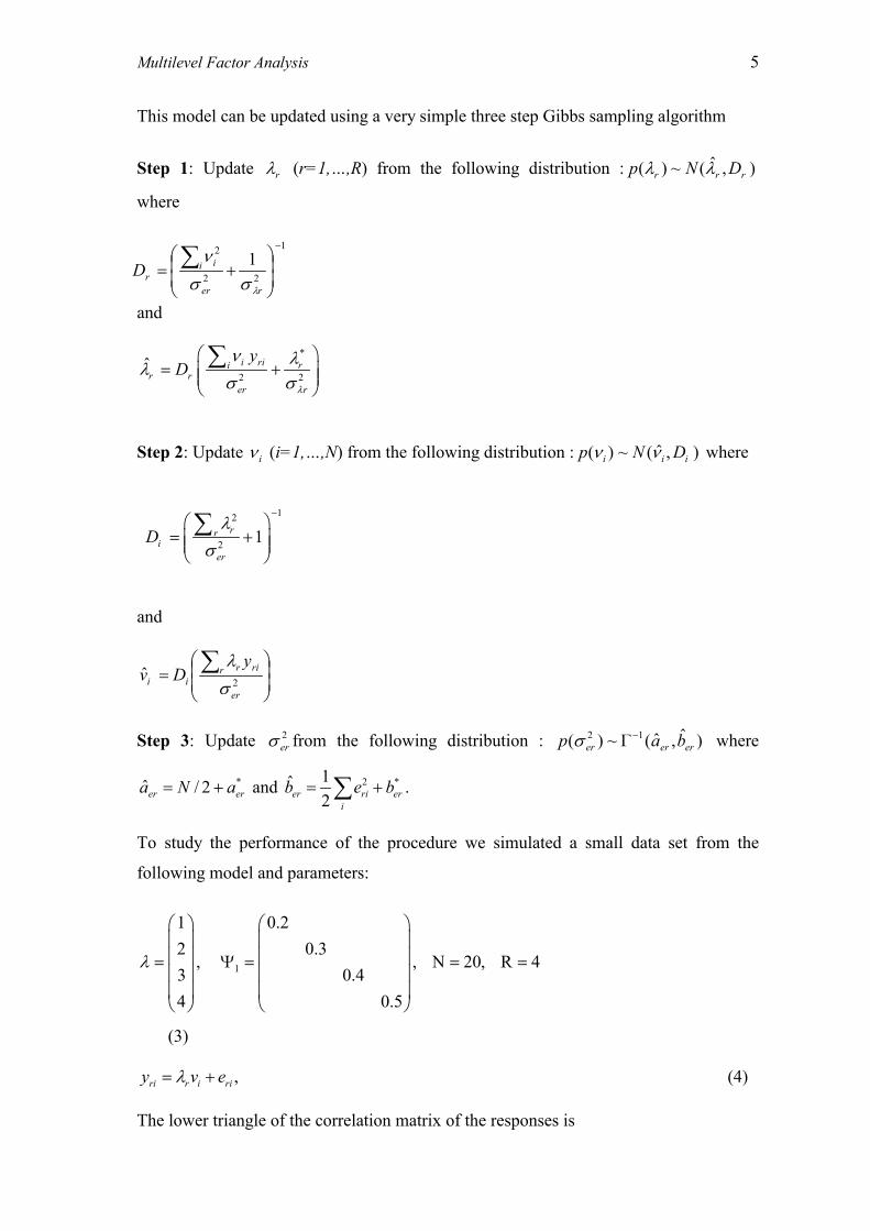
This model can be updated using a very simple three step Gibbs sampling algorithm
Step 1: Update � (r=1,…,R) from the following distribution :
where
r ),ˆ(~)( rrr DNp ��
1
22
2 1�
��
�
�
��
�
���
�
rer
i irD
���
�
and
*
2 2ˆ i ri rir r
er r
yD
�
� ��
� �
� �� �� �� �
� �
�
Step 2: Update � (i=1,…,N) from the following distribution :i ˆ( ) ~ ( , )i ip N D� � where
12
2 1rri
er
D�
�
�
� �� �� �� �� �
�
and
��
�
�
��
�
��
�2ˆer
r ririi
yDv
�
�
Step 3: Update � from the following distribution : where
and
2er )ˆ,ˆ(~)( 12
ererer bap �
��
*ˆ / 2er era N a� �2 *1
2er ri eri
b e� ��ˆ b
�
.
To study the performance of the procedure we simulated a small data set from the
following model and parameters:
1
1 0.22 0.3
, , N 20, R 43 0.44 0.5
�
� � � �� � � �� � � �� � � �� � � �� � � �� � � �
(3)
, ri r i riy v e�� � (4)
The lower triangle of the correlation matrix of the responses is

Multilevel Factor Analysis 6
10 93 10 92 0 97 1089 0 97 0 99 1
.
. .
. . .
�
�
����
�
�
����
All the variables have positively skewed distributions, and the chain loading estimates
also have highly significant positive skewness and kurtosis.
The initial starting value for each loading was 2 and for each level 1 variance
(uniqueness) was 0.2. Good starting values will speed up the convergence of the
MCMC chains.
Table 1 shows the maximum likelihood estimates produced by the AMOS factor
analysis package (Arbuckle, 1997) together with the MCMC results. The factor
analysis program carries out a prior standardisation so that the response variates have
zero means. In terms of the MCMC algorithm this is equivalent to adding covariates as
an 'intercept' term to (4), one for each response variable; these could be estimated by
adding an extra step to the above algorithm. Prior centring of the observed responses
can be carried out to improve convergence.
We have summarised the loading estimates by taking both the mean and medians of the
chain. The mode can also be computed, but in this data set for the variances it is very
poorly estimated and we give it only for the loadings. In fact the likelihood surface with
respect to the variances is very flat. The MCMC chains can be summarised using a
Normal kernel density smoothing method (Silverman 1986).

Multilevel Factor Analysis 7
Table 1. Maximum likelihood estimates for simulated data set together with MCMC estimates using chain length 50,000 burn in 20. Parameter ML estimate
(s.e.) MCMC mean estimates (s.d.)
MCMC median estimates
MCMC modal estimates
1� 0.92 (0.17) 1.03 (0.22) 1.00 0.98
2� 2.41 (0.41) 2.71 (0.52) 2.65 2.59
3� 3.86 (0.57) 3.91 (0.72) 3.82 3.71
4� 4.30 (0.71) 4.82 (0.90) 4.71 4.58
� e12 0.15 (0.05) 0.17 (0.07) 0.16
� e22 0.25 (0.09) 0.31 (0.14) 0.28
� e32 0.09 (0.10) 0.10 (0.17) 0.06
� e42 0.43 (0.20) 0.55 (0.31) 0.50
The estimates and standard errors from the MCMC chain are larger than the maximum
likelihood estimates. The standard errors for the latter will generally be underestimates,
especially for such a small data set since they use the estimated (plug in) parameter
values. The distributions for the variances in particular are skew so that median rather
than mean estimates seem preferable. Since we are sampling from the likelihood, the
maximum likelihood estimate will be located at the joint parameter mode. We have not
computed this but as can be seen from the loading estimates the univariate modes are
closer to the maximum likelihood estimates than the means or medians. Table 2 shows
good agreement between the variable means and the fitted intercept terms.
Table 2. Variable means and fitted intercepts
variable mean Intercept
1 0.54 0.57
2 0.64 0.71
3 1.12 1.21
4 1.28 1.36
We have also fitted the structure described by (3) and (4) with a simulated data set of
200 cases rather than 20. The results are given in table 3 for the maximum likelihood
estimates and the means and medians of the MCMC procedure.

Multilevel Factor Analysis 8
Table 3. Model (3) & (4) with 200 simulated individuals. 5000 cycles.
Parameter ML estimate (s.e.)
MCMC mean estimates (s.d.)
MCMC median estimates
MCMC mode
estimates
1� 0.95 (0.06) 0.97 (0.06) 0.96 0.96
2� 1.86 (0.10) 1.89 (0.10) 1.89 1.88
3� 2.92 (0.15) 2.98 (0.16) 2.97 2.97
4� 3.86 (0.20) 3.94 (0.20) 3.93 3.92
� e12 0.22 (0.023) 0.23 (0.024) 0.22 0.22
� e22 0.27 (0.033) 0.27 (0.033) 0.27 0.27
� e32 0.38 (0.058) 0.38 (0.060) 0.38 0.38
� e42 0.39 (0.085) 0.39 (0.087) 0.38 0.38
We see here a closer agreement. The MCMC estimates are slightly higher (by up to 2%)
than the maximum likelihood ones, with the modal estimates being closest.
In more complex examples we may need to run the chain longer with a longer burn in
and also try more than one chain with different starting values. For example, a
conventional single level factor model could be fitted using standard software to obtain
approximations to the level 1 loadings and unique variances.
Other procedures
Geweke and Zhou (1996) consider the single level factor model with uncorrelated
factors. They use Gibbs sampling and consider identifiability constraints. Zhu and Lee
(1999) also consider single level structures including non-linear models that involve
factor products and powers of factors. They use Gibbs steps for the parameters and a
Metropolis Hastings algorithm for simulating from the conditional distribution of the
factors. They also provide a goodness-of-fit criterion (see discussion). It appears,
however, that their algorithm requires individuals to have complete data vectors with no
missing responses, whereas the procedure described in the present paper has no such
restriction.
Scheines et al (1999) also use MCMC and take as data the sample covariance matrix,
for a single level structure, where covariates are assumed to have been incorporated into
the means. They assume a multivariate Normal prior with truncation at zero for the

Multilevel Factor Analysis 9 variances. Rejection sampling is used to produce the posterior distribution. They
discuss the problem of identification, and point out that identification issues may be
resolved by specifying an informative prior.
McDonald and Goldstein (1989) show how maximum likelihood estimates can be
obtained for a 2-level structural equation model. They derive the covariance structure
for such a model and show how an efficient algorithm can be constructed to obtin
maximum likelihood estimates for the multivariate Normal case. Longford and Muthen
(1992) develop this approach. The latter authors, together with Goldstein (1995,
Chapter 11) and Rowe and Hill (1997, 1998) also point out that consistent estimators
can be obtained from a 2-stage process as follows. A 2-level multivariate response
linear model is fitted using an efficient procedure such as maximum likelihood. This
can be accomplished, for example as pointed out earlier by defining a 3-level model
where the lowest level is that of the response variables (see Goldstein, 1995, Chapter 8
and model (5) below). This analysis will produce estimates for the (residual) covariance
matrices at each level and each of these can then be structured according to an
underlying latent variable model in the usual way. By considering the two matrices as
two ‘populations’ we can also impose constraints on, say, the loadings using an
algorithm for simultaneously fitting structural equations across several populations.
Rabe-Hesketh et al. (2000) consider a general formulation, similar to model (7) below,
but allowing general link functions, to specify multilevel structural equation generalised
linear models (GLLAMM). They consider maximum likelihood estimation using
general maximisation algorithms and a set of macros has been written to implement the
model in the program STATA.
In the MCMC formulation in this paper, it is possible to deal with incomplete data
vectors and also to use informative prior distributions, as described below. Our
algorithm can also be extended to the non-linear factor case using a Metropolis Hastings
step when sampling the factor values, as in Zhu and Lee (1999).
General multilevel Bayesian factor models
Extensions to models with further factors, patterned loading matrices and higher levels
in the data structure are straightforward. We will consider the 2-level factor model

Multilevel Factor Analysis 10
)
(2) (2) (1) (1)
1 1
2 2 (2) (1)2 1
1
~ (0, ), ~ (0, ), ~ (0, ), ~ (0, )
1,..., , 1,..., , 1,..., ,
F G
rij r fr fj gr gij rj rijf g
rj ur rij er fj F gij G
J
j jj
y u e
u N e N MVN MVN
r R i n j J n N
� � � � �
� � � �
� �
�
� � � � �
� �
� � � �
� �
�
Here we have R responses for N individuals split between J level 2 units. We have F
sets of factors, � defined at level 2 and G sets of factors, � defined at level 1. For
the fixed part of the model we restrict our algorithm to a single intercept term for
each response although it is easy to extend the algorithm to arbitrary fixed terms. The
residuals at levels 1 and 2, e
)2(fj
)1(gij
r�
rij and urj are assumed to be independent.
Although this allows a very flexible set of factor models it should be noted that in order
for such models to be identifiable suitable constraints must be put on the parameters.
See Everitt (1984) for further discussion of identifiability.
These will consist of fixing the values of some of the elements of the factor variance
matrices, �1 and �2 and/or some of the factor loadings, � and . )2(fr
)1(gr�
The algorithms presented will give steps for all parameters and so any parameter that is
constrained will simply maintain its chosen value and will not be updated. We will
initially assume that the factor variance matrices, �1 and �2 are known (completely
constrained) and then discuss how the algorithm can be extended to encompass partially
constrained variance matrices. The parameters in the following steps are those available
at the current iteration of the algorithm.
Prior Distributions
For the algorithm we will assume the following general priors
* 2
(2) (2)* 2 (1) (1)* 22 1
2 1 * * 2 1 * *
( ) ~ ( , )
( ) ~ ( , ), ( ) ~ ( ,
( ) ~ ( , ), ( ) ~ ( , )
r r br
fr fr fr gr gr gr
ur ur ur er er er
p N
p N p N
p a b p a b
� � �
� � � � � �
� �� �
� �

Multilevel Factor Analysis 11 As we are assuming that the factor variance matrices are known we can use a Gibbs
sampling algorithm which will involve updating parameters in turn by generating new
values from the following 8 sets of conditional posterior distributions.
Step 1: Update current value of (r=1,…,R) from the following distribution r�
),ˆ(~)( brrr DNp �� where
1
2 2
1br
er br
ND� �
�
� �� �� �� �
and
*
2 2ˆ rijij r
r brer br
dD
�
��
� �
� �� �� �
� �� �
�
where
rrijrij ed ����
Step 2: Update (r=1,…,R, f =1,…,F where not constrained) from the following
distribution : where
)2(fr�
~))2(fr ),ˆ(( )2()2(
frfr DNp ��
1(2) 2(2)
2 22
( ) 1j fjjfr
er fr
nD
�
� �
�
� �� �� �� �� �
�
and
(2) (2) (2)*(2) (2)
2 22
ˆ fj rijfij frfr fr
er fr
dD
� ��
� �
� �� �� �
� �� �
�
where
)2()2()2(fjfrrijrijf ved ���

Multilevel Factor Analysis 12 Step 3: Update � (r=1,…,R, g =1,…,G where not constrained) from the following
distribution : where
)1(gr
))1(gr ),ˆ(~( )1()1(
grgr DNp ��
1(1) 2(1)
2 21
( ) 1gijijgr
er gr
D�
� �
�
� �� �� �� �� �
�
and
(1) (1) (1)*(1) (1)
2 21
ˆ gij rijgij grgr gr
er gr
dD
� ��
� �
� �� �� �� �� �
�
where
)1()1()1(gijgrrijrijg ved ���
Step 4: Update � ( j= 1,…,J) from the following distribution:
where
)2(j
))2(j,ˆ(~)( )2()2(
jFj DMVNp ��
1(2) (2)(2) 1
22
( )Tj r r
jr er
nD
� �
�
�
�
� �� �� �� �� � �
and
(2) (2)(2) (2)
21
ˆjn
r rijj j
r i er
dD
��
��
� �� � �� �
� ���
where
��
����
F
f
TFjjj
TFrrrfjfrrijrij vvvved
1
)2()2(1
)2()2()2(1
)2()2()2()2( ),...,( ,),....( , ����
Step 5: Update � ( i=1,…,n)1(ij
(G
j, j= 1,…,J) from the following
distribution: where ),ˆ~)( )1()1()1(ijijij DMVNp ��

Multilevel Factor Analysis 13
11
12
)1()1()1( )(
�
�
���
����
��� �
er
Trr
rijD
�
��
and
(1) (1)(1) (1)
2ˆ r rij
j ijr er
dD
��
�
� �� � �� �
� ��
where
��
����
G
g
TGijijij
TGrrrgjgrrijrij vvvved
1
)1()1(1
)1()1()1(1
)1()1()1()1( ),...,( ,),....( , ����
Step 6: Update u (r=1,…,R, j=1,…,J) from the following distribution :
where
rj
),ˆ(~)( )(urjrjrj DuNup
1( )
2 2
1jurj
er ur
nD
� �
�
� �� �� �� �
and
( )( )
21
ˆju n
rj urj rij
ier
Du d
��
� �
where
rjriju
rij ued ��)(
Step 7: Update � from the following distribution : where
and
2ur )ˆ,ˆ(~)( 12
ururur bap �
��
*ˆ / 2ur ura J a� �2 *1
2 rj urj
b u� ��ur b .
Step 8: Update � from the following distribution : where
and
2er )ˆ,ˆ(~)( 12
ererer bap �
��
*ˆ / 2er era N a� �2 *1
2er rij erij
b e� ��ˆ b .

Multilevel Factor Analysis 14 Note that the level 1 residuals, can be calculated by subtraction at every step of the
algorithm.
rije
Unconstrained Factor Variance Matrices
In the general algorithm we have assumed that the factor variances are all constrained.
Typically we will fix the variances to equal 1 and the covariances to equal 0 and have
independent factors. This form will allow us to simplify steps 4 and 5 of the algorithm
to univariate Normal updates for each factor separately. We may however wish to
consider correlations between the factors. Here we will modify our algorithm to allow
another special case where the variances are constrained to be 1 but the covariances can
be freely estimated. Where the resulting correlations obtained are estimated to be close
to 1 or –1 then we may be fitting too many factors at that particular level. As the
variances are constrained to equal 1 the covariances between factors equal the
correlations between the factors. This means that each covariance is constrained to lie
between –1 and 1. We will consider here only the factor variance matrix at level 2 as the
step for the level 1 variance matrix simply involves changing subscripts. We will use
the following priors:
2,( ) ~ ( 1,1)lmp Uniform l m� � � �
Here is the l,m-th element of the level 2 factor variance matrix. We will update
these covariance parameters using a Metropolis step and a Normal random walk
proposal (see Browne and Rasbash (in preparation) for more details on using Metropolis
Hastings methods for constrained variance matrices).
lm,2�
Step 9 : At iteration t generate ~ N( ) where � is a proposal
distribution variance that has to be set for each covariance. Then if > 1 or < -
1 set =� as the proposed covariance is not valid else form a proposed new
matrix � by replacing the l,m th element of � by this proposed value. We then set
*,2 lm�
2)1(,2 , plmtlm ��
�
)1(2�t
2plm
*,2 lm�
*,2 lm�
)(,2tlm�
*2
)1(,2�tlm

Multilevel Factor Analysis 15
)(,2tlm�
)(,2tlm�
= with probability min(1, and
= otherwise.
*,2 lm�
)1(,2�
�tlm
)|(/)|( )2()1(2
)2(*2 fj
tfj pp ��
�
��
Here and ))()(exp(||)|( )2(1*2
)2(2/1*2
)2(*2 fj
Tfj
jfjp ���
��
���� �
))()(exp(||)|( )2(1)1(2
)2(2/1)1(2
)2()1(2 fj
tTfj
j
tfj
tp ��������
���� �
This procedure is repeated for each covariance that is not constrained.
Missing Data
The exam example that is discussed in this paper has the additional difficulty that
individuals have different numbers of responses. This is not a problem for the MCMC
methods if we are prepared to assume missingness is at random or effectively so by
design. This is equivalent to giving the missing data a uniform prior. We then have to
simply add an extra Gibbs sampling step to the algorithm to sample the missing values
at each iteration. As an illustration we will consider an individual who is missing
response r. In a factor model the correlation between responses is explained in the factor
terms and conditional on these terms the responses for an individual are independent
and so the conditional distributions of the missing responses have simple forms.
Step 10: Update (r=1,…,R, i=1,…,nrijy
��
G
ggr
1
1(�
j, j=1,…,J � that are missing) from the
following distribution, given the current values, where =
.
rijy
rijy ),ˆ(~ 2errijyN � rijy
��
��� rjgij
F
ffjfrr u)1()
1
)2()2( ����
Example
The example uses a data set discussed by Goldstein (1995, Chapter 4) and consists of a
set of responses to a series of 4 test booklets by 2439 pupils in 99 schools. Each student
responded to a core booklet containing Earth science, biology and physics items and to
a further two booklets randomly chosen from three available. Two of these booklets
were in biology and one in physics. As a result there are 6 possible scores, one in earth

Multilevel Factor Analysis 16 science, three in biology and 2 in physics, each student having up to five. A full
description of the data is given in Goldstein (1995).
A multivariate 2-level model fitted to the data gives the following maximum likelihood
estimates for the means and covariance/correlation matrices in Table 4. The model can
be written as follows
6 6 6 6
1 1 1 1
1 1
2 2
3 3
4 4
5 5
6 6
~ (0, ) ~ (0, )
1 if , 0 otherwise1 if a girl, 0 if a boy
ijk i hjk i hjk jk ijk hjk ik hjkh h h h
u v
hjk
jk
y x x z u x v x
u vu vu v
N Nu vu vu v
x h izi
� �� � � �
� � � �
� � � �� � � �� � � �� � � �
� �� � � �� � � �� � � �� � � �� � � �� �
� �
� �
� � � �
indexes response variables, indexes students, indexes schoolsj k
(5)

Multilevel Factor Analysis 17 Table 4. Science attainment estimates. Fixed Estimate (s.e.) Earth Science Core 0.838 (0.0076) Biology Core 0.711 (0.0100) Biology R3 0.684 (0.0109) Biology R4 0.591 (0.0167) Physics Core 0.752 (0.0128) Physics R2 0.664 (0.0128) Earth Science Core (girls - boys) -0.0030 (0.0059) Biology Core (girls - boys) -0.0151 (0.0066) Biology R3 (girls - boys) 0.0040 (0.0125) Biology R4 (girls - boys) -0.0492 (0.0137) Physics Core (girls - boys) -0.0696 (0.0073) Physics R2 (girls - boys) -0.0696 (0.0116) Random. Variances on diagonal; correlations off-diagonal Level 2 (School)
E.Sc. core Biol. Core Biol R3 Biol R4 Phys. core Phys. R2 E.Sc. core 0.0041 Biol. core 0.68 0.0076 Biol R3 0.51 0.68 0.0037 Biol R4 0.46 0.68 0.45 0.0183 Phys. core 0.57 0.90 0.76 0.63 0.0104 Phys. R2 0.54 0.78 0.57 0.65 0.78 0.0095 Level 1 (Student)
E.Sc. core Biol. Core Biol R3 Biol R4 Phys. core Phys. R2 E.Sc. core 0.0206 Biol. core 0.27 0.0261 Biol R3 0.12 0.13 0.0478 Biol R4 0.14 0.27 0.20 0.0585 Phys. core 0.26 0.42 0.11 0.27 0.0314 Phys. R2 0.22 0.33 0.14 0.37 0.41 0.0449
We now fit two 2 level factor models to these data, shown in Table 5. We omit the fixed
effects in Table 5 since they are very close to those in Table 4. Model A has two factors
at level 1 and a single factor at level 2. For illustration we have constrained all the
variances to be 1.0 and allowed the covariance (correlation) between the level 1 factors
to be estimated. Inspection of the correlation structure suggests a model where the first
factor at level 1 estimates the loadings for Earth Science and Biology, constraining
those for Physics to be zero (the physics responses have the highest correlation), and for
the second factor at level 1 to allow only the loadings for Physics to be unconstrained.
The high correlation of 0.90 between the factors suggests that perhaps a single factor
will be an adequate summary. Although we do not present results, we have also studied

Multilevel Factor Analysis 18 a similar structure for two factors at the school level where the correlation is estimated
to be 0.97, strongly suggesting a single factor at that level.
For model B we have separated the three topics of Earth Science, Biology and Physics
to separately have non-zero loadings on three corresponding factors at the student level.
This time the high inter-correlation is that between the Biology and Physics booklets
with only moderate (0.49, 0.55) correlations between Earth Science and Biology and
Physics. This suggests that we need at least two factors to describe the student level data
and that our preliminary analysis suggesting just one factor can be improved. Since our
analyses are for illustrative purposes only we have not pursued further possibilities with
these data.

Multilevel Factor Analysis 19 Table 5. Science attainment MCMC factor model estimates. Parameter A Estimate (s.e.) B Estimate (s.e.) Level 1; factor 1 loadings E.Sc. core 0.06 (0.004) 0.11 (0.02) Biol. core 0.11 (0.004) 0* Biol R3 0.05 (0.008) 0* Biol R4 0.11 (0.009) 0* Phys. core 0* 0* Phys. R2 0* 0* Level 1; factor 2 loadings E.Sc. core 0* 0* Biol. core 0* 0.10 (0.005) Biol R3 0* 0.05 (0.008) Biol R4 0* 0.10 (0.009) Phys. core 0.12 (0.005) 0* Phys. R2 0.12 (0.007) 0* Level 1; factor 3 loadings E.Sc. core - 0* Biol. core - 0* Biol R3 - 0* Biol R4 - 0* Phys. core - 0.12 (0.005) Phys. R2 - 0.12 (0.007) Level 2; factor 1 loadings E.Sc. core 0.04 (0.007) 0.04 (0.007) Biol. core 0.09 (0.008) 0.09 (0.008) Biol R3 0.05 (0.009) 0.05 (0.010) Biol R4 0.10 (0.016) 0.10 (0.016) Phys. core 0.10 (0.010) 0.10 (0.010) Phys. R2 0.09 (0.011) 0.09 (0.011) Level 1 residual variances E.Sc. core 0.017 (0.001) 0.008 (0.004) Biol. core 0.015 (0.001) 0.015 (0.001) Biol R3 0.046 (0.002) 0.046 (0.002) Biol R4 0.048 (0.002) 0.048 (0.002) Phys. core 0.016 (0.001) 0.016 (0.001) Phys. R2 0.029 (0.002) 0.030 (0.002) Level 2 residual variances E.Sc. core 0.002 (0.0005) 0.002 (0.0005) Biol. core 0.0008 (0.0003) 0.0008 (0.0003) Biol R3 0.002 (0.0008) 0.002 (0.0008) Biol R4 0.010 (0.002) 0.010 (0.002) Phys. core 0.002 (0.0005) 0.002 (0.0005) Phys. R2 0.003 (0.0009) 0.003 (0.0009) Level 1 correlation factors 1 &2 0.90 (0.03) 0.55 (0.10) Level 1 correlation factors 1 &3 - 0.49 (0.09) Level 1 correlation factors 2 &3 - 0.92 (0.04) * indicates constrained parameter. A chain of length 20,000 with a burn in of 2000 was used. Level 1 is student, level 2 is school.
Discussion
This paper has shown how factor models can be specified and fitted. The MCMC
computations allow point and interval estimation with an advantage over maximum
Multilevel Factor Analysis 20
2 2
2 )
likelihood estimation in that full account is taken of the uncertainty associated with the
estimates. In addition it allows full Bayesian modelling with informative prior
distributions which may be especially useful for identification problems.
As pointed out in the introduction, the MCMC algorithm is readily extended to handle
the general structural equation case, and further work is being carried out along the
following lines. For simplicity we consider the single level model case to illustrate the
procedure.
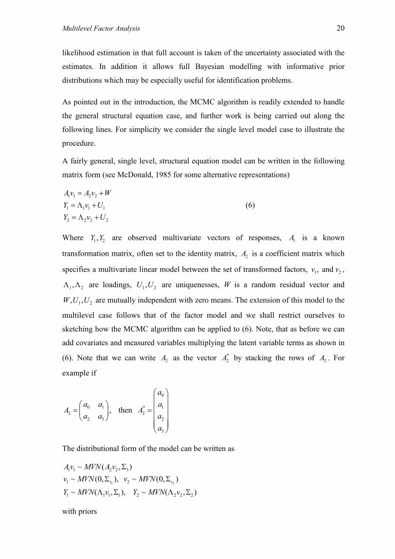
A fairly general, single level, structural equation model can be written in the following
matrix form (see McDonald, 1985 for some alternative representations)
1 1 2 2
1 1 1 1
2 2 2 2
A v A v WY v UY v U
� �
� � �
� � �
(6)
Where are observed multivariate vectors of responses, is a known
transformation matrix, often set to the identity matrix, is a coefficient matrix which
specifies a multivariate linear model between the set of transformed factors, ,
are loadings, U U are uniquenesses, W is a random residual vector and
are mutually independent with zero means. The extension of this model to the
multilevel case follows that of the factor model and we shall restrict ourselves to
sketching how the MCMC algorithm can be applied to (6). Note, that as before we can
add covariates and measured variables multiplying the latent variable terms as shown in
(6). Note that we can write as the vector by stacking the rows of . For
example if
Y Y1 2,
2
1A
2A
1 2, and v v
2A
� �1,
W U, ,1
1,
U
2A *2A
0
0 1 1*2 2
2 3 2
3
, then
aa a a
A Aa a a
a
� �� �
� � � �� �� � � �� �� �� �� �
The distributional form of the model can be written as
1 2
1 1 2 2 3
1 2
1 1 1 1 2 2 2
~ ( , )~ (0, ), ~ (0, )
~ ( , ), ~ ( ,v v
A v MVN A vv MVN v MVN
Y MVN v Y MVN v
�
� �
� � � �
with priors

Multilevel Factor Analysis 21
)* 1 22
* *2 2 1 1 2 2
ˆ ˆ ˆ ~ ( , ), ~ ( , ), ~ ( ,A
A MVN A MVN MVN� �
� � � � � � �
and having inverse Wishart priors. 1 2 3, ,� � �
The coefficient and loading matrices have conditional Normal distributions as do the
factor values. The covariance matrices and uniqueness variance matrices involve steps
similar to those given in the earlier algorithm. The extension to two levels and more
follows the same general procedure as we have shown earlier.
The model can be generalised further by considering m sets of response variables,
in (6) and several, linked, multiple group structural relationships with the k-
th relationship having the general form
Y Y Ym1 2, ,...
V A V A Whk
hk
hg
kg
k k
g
( ) ( ) ( ) ( ) ( )� �� �
and the above procedure can be extended for this case. We note that the model for
simultaneous factor analysis (or, more generally, structural equation model) in several
populations is a special case of this model, with the addition of any required constraints
on parameter values across populations.
We can also generalise (1) to include fixed effects, responses at level 2 and covariates
hZ for the factors, which may be a subset of the fixed effects covariates X
(1) (1) (1) (1) (1) (1)2 2 2 1 1 1
(2) (2) (2) (2)2 2 2
(1) (2){ }, { }1,..., 1,..., 1,...,
rij rj
j
Y X v Z u v Z eY v Z uY y Y yr R i i j J
�� � � � � � �
� � �
� �
� � �
(7)
The superscript refers to the level at which the measurement exists, so that, for example,
refer respectively to the first measurement in the i-th level 1 unit in the j-th
level 2 unit (say students and schools) and the second measurement taken at school
level for the j-th school.
1 2, ij jy y
Further work is currently being carried out on applying these procedures to non-linear
models and specifically to generalised linear models. For simplicity consider the
binomial response logistic model as illustration. Write

Multilevel Factor Analysis 22
)
1
ij
( ) [1 exp ( )]
~Bin( , ) ij ij i i j
ij ij
E y a v
y n
� �
�
�
� � � � �
(8)
The simplest model is the multiple binary response model ( ) that is referred to in
the psychometric literature as a unidimensional item response model (Goldstein &
Wood, 1989, Bartholomew and Knott, 1999). Estimation for this model is not possible
using a simple Gibbs sampling algorithm but as in the standard binomial multilevel case
(see Browne, 1998) we could replace any Gibbs steps that do not have standard
conditional posterior distributions with Metropolis Hastings steps.
nij � 1
The issues that surround the specification and interpretation of single level factor and
structural equation models are also present in our multilevel versions. Parameter
identification has already been discussed; another issue is the boundary ‘Heywood’
case. We have observed such solutions occurring where sets of loading parameters tend
towards zero or a correlation tends towards 1.0. A final important issue that only affects
stochastic procedures is the problem of ‘flipping states’. This means that there is not a
unique solution even in a 1-factor problem as the loadings and factor values may all flip
their sign to give an equivalent solution. When the number of factors increases there are
greater problems as factors may swap over as the chains progress. This means that
identifiability is an even greater consideration when using stochastic techniques.
For making inferences about individual parameters or functions of parameters we can
use the chain values to provide point and interval estimates. These can also be used to
provide large sample Wald tests for sets of parameters. Zhu and Lee propose a chi-
square discrepancy function for evaluating the posterior predictive p-value, which is the
Bayesian counterpart of the frequentist p-value statistic (Meng, 1994). In the multilevel
case the � probability becomes level�
1 2 ( ) (
1 1
1( ) ( )
ˆ ˆ( ) ( ) ( ) ( | , )
ˆ( | , )
jiJi i
B j j ii i
i i Ti i i i
p Y i i p D Y v
D Y v Y Y
�� �
�
�
� �
�
� �
� �
� � (9)
where is the vector of responses for the i-th level 2 unit and � is the (non-diagonal)
residual covariance matrix.
iY i
Multilevel Factor Analysis 23
References
Arbuckle, J.L. (1997). AMOS: Version 3.6. Chicago: Small Waters Corporation.
Bartholomew, D.J. and Knott, M. (1999). Latent variable models and factor analysis.
(2nd edition). London, Arnold.
Browne, W. (1998). Applying MCMC methods to multilevel models. PhD thesis,
University of Bath.
Browne, W. and Rasbash, J. (2001). MCMC algorithms for variance matrices with
applications in multilevel modeling. (in preparation)
Blozis, S. A. and Cudeck, R. (1999). Conditionally linear mixed-effects models with
latent variable covariates. Journal of Educational and Behavioural Statistics 24:
245-270.
Clayton, D. and Rasbash, J. (1999). Estimation in large crossed random effect models
by data augmentation. Journal of the Royal Statistical Society, A. 162: 425-36.
Everitt, B. S. (1984). An introduction to latent variable models. London, Chapman and
Hall.
Geweke, J. and Zhou, G. (1996). Measuring the pricing error of the arbitrage pricing
theory. The review of international financial studies 9: 557-587.
Goldstein, H. (1995). Multilevel statistical models. London: Edward Arnold.
Goldstein, H., & McDonald, R.P. (1988). A general model for the analysis of
multilevel data. Psychometrika, 53 (4), 455-467.
Goldstein, H., & Rasbash, J. (1996). Improved approximations for multilevel models
with binary responses. Journal of the Royal Statistical Society, A. 159, 505-13.
Goldstein, H., Rasbash, J., Plewis, I., Draper, D., Browne, W., Yang, M., Woodhouse,
G., & Healy, M. (1998). A user’s guide to MLwiN. Multilevel Models Project,
Institute of Education University of London.
Goldstein, H., & Wood, R. (1989). Five decades of item response modelling. British
Journal of Mathematical and Statistical Psychology, 42, 139-167.
Multilevel Factor Analysis 24 Lindsey, J. K. (1999). Relationships among sample size, model selection and likelihood
regions, and scientifically important differences. Journal of the Royal Statistical
Society, D 48: 401-412.
Longford, N., & Muthen, B. O. (1992). Factor analysis for clustered observations.
Psychometrika, 57, 581-597.
Mcdonald, R. P. (1985). Factor analysis and related methods. Hillsdale, NJ, Lawrence
Earlbaum.
McDonald, R. P. (1993). A general model for two-level data with responses missing at
random. Psychometrika, 58, 575-585.
McDonald, R.P., & Goldstein, H. (1989). Balanced versus unbalanced designs for
linear structural relations in two-level data. British Journal of Mathematical and
Statistical Psychology, 42, 215-232.
Meng, X. L. (1994). Posterior predictive p-values. Annals of Statistics 22: 1142-1160.
Rabe-hesketh, S., Pickles, A. and Taylor, C. (2000). Sg129: Generalized linear latent
and mixed models. Stata technical bulletin 53, 47-57.
Rasbash, J., Browne, W., Goldstein, H., Yang, M., et al. (2000). A user's guide to
MlwiN (Second Edition). London, Institute of Education:
Raudenbush, S.W. (1995). Maximum Likelihood estimation for unbalanced multilevel
covariance structure models via the EM algorithm. British Journal of
Mathematical and Statistical Psychology, 48, 359-70.
Rowe, K.J., & Hill, P.W. (1997). Simultaneous estimation of multilevel structural
equations to model students' educational progress. Paper presented at the Tenth
International Congress for School effectiveness and School Improvement,
Memphis, Tennessee.
Rowe, K.J., & Hill, P.W. (1998). Modelling educational effectiveness in classrooms:
The use of multilevel structural equations to model students’ progress.
Educational Research and Evaluation, 4 (to appear).
Rubin, D.B., & Thayer, D. T. (1982). EM algorithms for ML factor analysis.
Psychometrika, 47, 69-76.
Scheines, R., Hoijtink, H. and Boomsma, A. (1999). Bayesian estimation and testing of
structural equation models. Psychometrika 64: 37-52.

Multilevel Factor Analysis 25 Silverman, B.W. (1986). Density Estimation for Statistics and Data analysis. London:
Chapman and Hall.
Zhu, H.-T. and Lee, S.-Y. (1999). Statistical analysis of nonlinear factor analysis
models. British Journal of Mathematical and Statistical Psychology 52: 225-242.


