
Multispectral and Hyper spectral remote sensing and its applications
Agricultural College, Bapatla
Class seminar on
By
Medida Sunil Kumar
BAD-14-06
1
Introduction
• Natural color image data is comprised of red, green, and
blue bands.
• Color infrared data is comprised of infrared, red, and
green bands.
• For multispectral data containing more than 3 spectral
bands, the user must choose a subset of 3 bands to display
at any given time
Multispectral image
Multispectral imagery generally refers to 3 to 10 bands that are
represented in pixels. Each band is acquired using a remote sensing
radiometer.
Examples of MSS sensors
Multispectral Imaging using discrete detectors and scanning mirrors
Landsat Multispectral Scanner (MSS)
Landsat Thematic Mapper (TM)
NOAA Advanced Very High Resolution Radiometer (AVHRR)
NASA and ORBIMAGE, Inc., Sea-viewing Wide field-of-view Sensor
(SeaWiFS)
Daedalus, Inc., Aircraft Multispectral Scanner (AMS)
NASA Airborne Terrestrial Applications Sensor (ATLAS)
Multispectral Imaging Using Linear Arrays
SPOT 1, 2, and 3 High Resolution Visible (HRV) sensors and Spot 4 and 5 High
Resolution Visible Infrared (HRVIR) and vegetation sensor
Indian Remote Sensing System (IRS) Linear Imaging Self-scanning Sensor
(LISS)
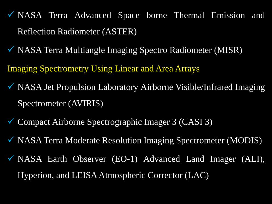
NASA Terra Advanced Space borne Thermal Emission and
Reflection Radiometer (ASTER)
NASA Terra Multiangle Imaging Spectro Radiometer (MISR)
Imaging Spectrometry Using Linear and Area Arrays
NASA Jet Propulsion Laboratory Airborne Visible/Infrared Imaging
Spectrometer (AVIRIS)
Compact Airborne Spectrographic Imager 3 (CASI 3)
NASA Terra Moderate Resolution Imaging Spectrometer (MODIS)
NASA Earth Observer (EO-1) Advanced Land Imager (ALI),
Hyperion, and LEISA Atmospheric Corrector (LAC)
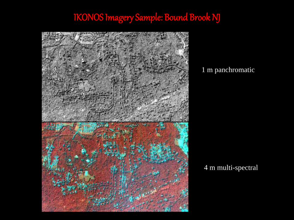
4 m multi-spectral
1 m panchromatic
IKONOS Imagery Sample: Bound Brook NJ
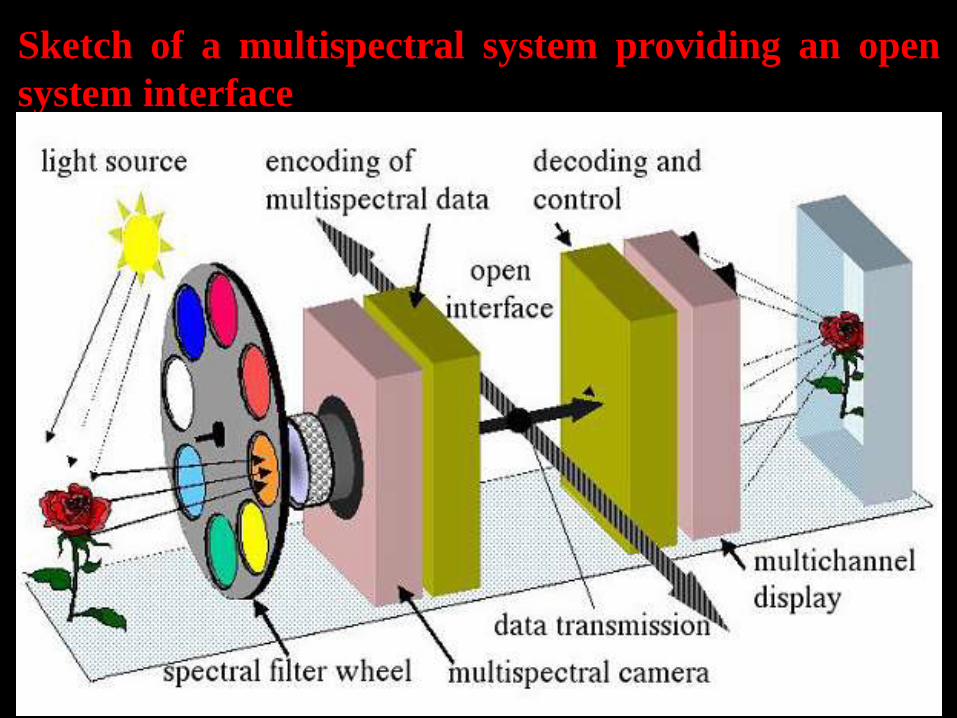
Sketch of a multispectral system providing an open
system interface
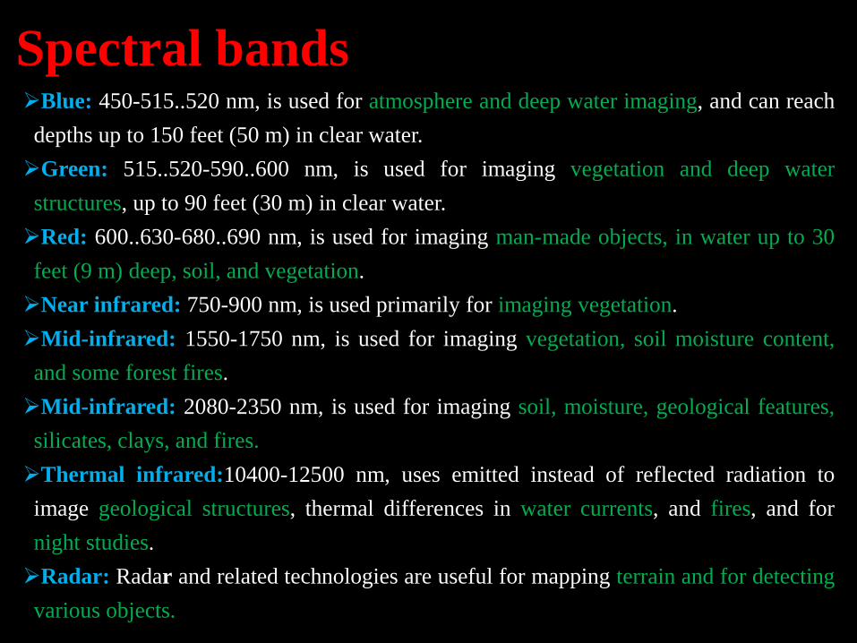
Spectral bandsBlue: 450-515..520 nm, is used for atmosphere and deep water imaging, and can reach
depths up to 150 feet (50 m) in clear water.
Green: 515..520-590..600 nm, is used for imaging vegetation and deep water
structures, up to 90 feet (30 m) in clear water.
Red: 600..630-680..690 nm, is used for imaging man-made objects, in water up to 30
feet (9 m) deep, soil, and vegetation.
Near infrared: 750-900 nm, is used primarily for imaging vegetation.
Mid-infrared: 1550-1750 nm, is used for imaging vegetation, soil moisture content,
and some forest fires.
Mid-infrared: 2080-2350 nm, is used for imaging soil, moisture, geological features,
silicates, clays, and fires.
Thermal infrared:10400-12500 nm, uses emitted instead of reflected radiation to
image geological structures, thermal differences in water currents, and fires, and for
night studies.
Radar: Radar and related technologies are useful for mapping terrain and for detecting
various objects.
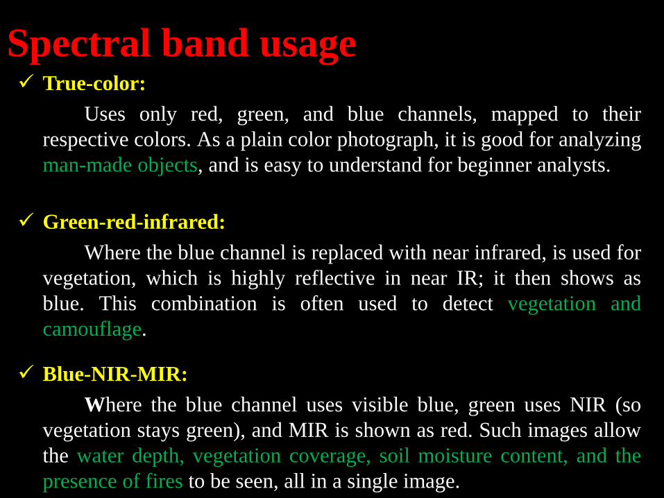
Spectral band usage True-color:
Uses only red, green, and blue channels, mapped to their
respective colors. As a plain color photograph, it is good for analyzing
man-made objects, and is easy to understand for beginner analysts.
Green-red-infrared:
Where the blue channel is replaced with near infrared, is used for
vegetation, which is highly reflective in near IR; it then shows as
blue. This combination is often used to detect vegetation and
camouflage.
Blue-NIR-MIR:
Where the blue channel uses visible blue, green uses NIR (so
vegetation stays green), and MIR is shown as red. Such images allow
the water depth, vegetation coverage, soil moisture content, and the
presence of fires to be seen, all in a single image.
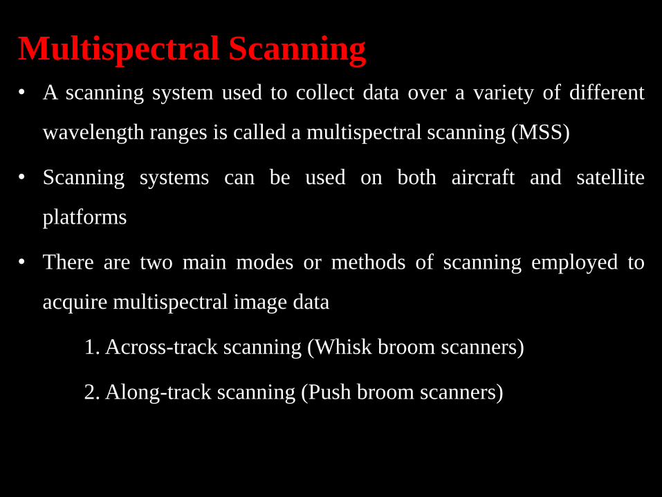
Multispectral Scanning
• A scanning system used to collect data over a variety of different
wavelength ranges is called a multispectral scanning (MSS)
• Scanning systems can be used on both aircraft and satellite
platforms
• There are two main modes or methods of scanning employed to
acquire multispectral image data
1. Across-track scanning (Whisk broom scanners)
2. Along-track scanning (Push broom scanners)
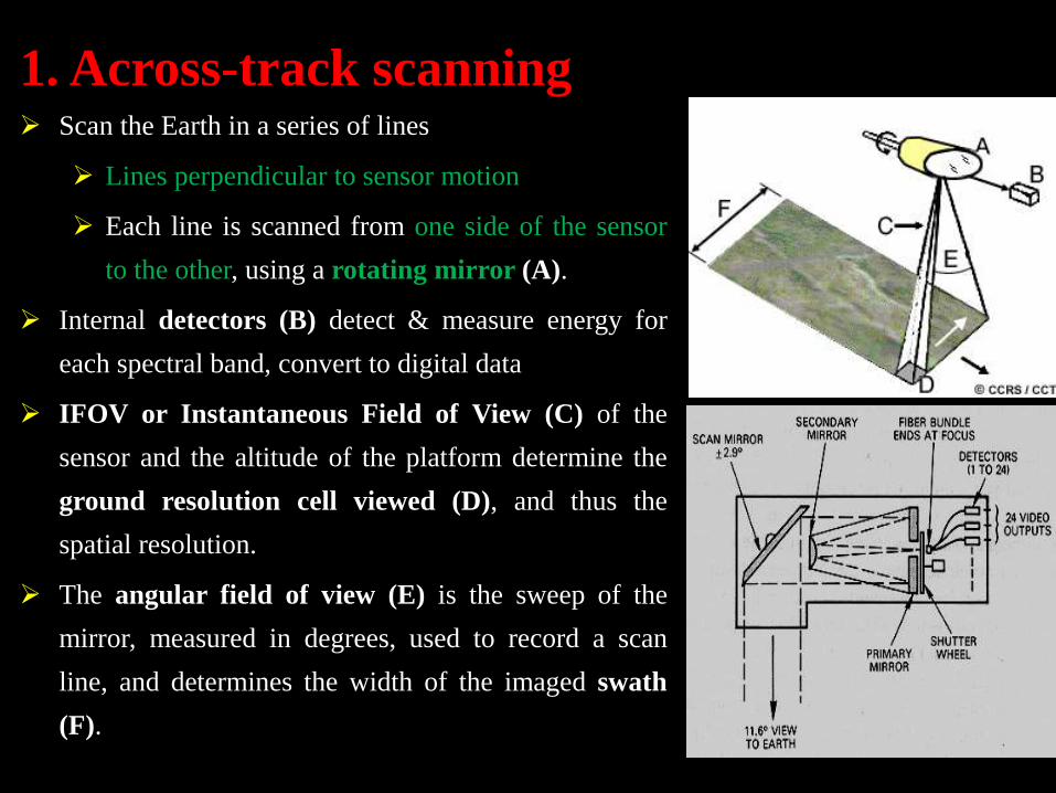
1. Across-track scanning Scan the Earth in a series of lines
Lines perpendicular to sensor motion
Each line is scanned from one side of the sensor
to the other, using a rotating mirror (A).
Internal detectors (B) detect & measure energy for
each spectral band, convert to digital data
IFOV or Instantaneous Field of View (C) of the
sensor and the altitude of the platform determine the
ground resolution cell viewed (D), and thus the
spatial resolution.
The angular field of view (E) is the sweep of the
mirror, measured in degrees, used to record a scan
line, and determines the width of the imaged swath
(F).
http://ccrs.nrcan.gc.ca/resource/tutor/fundam/chapter2/08_e.php
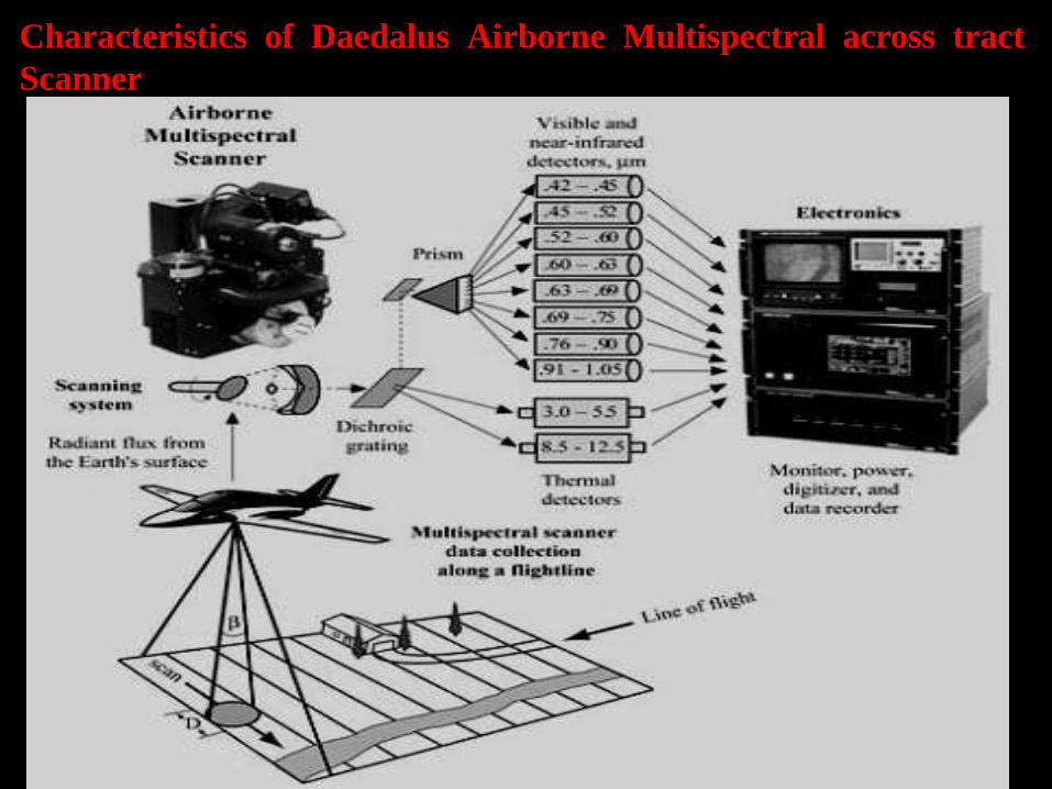
Characteristics of Daedalus Airborne Multispectral across tract
Scanner
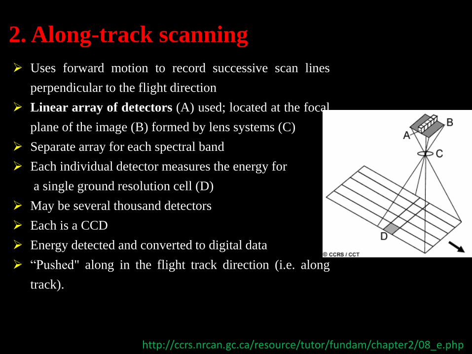
2. Along-track scanning
Uses forward motion to record successive scan lines
perpendicular to the flight direction
Linear array of detectors (A) used; located at the focal
plane of the image (B) formed by lens systems (C)
Separate array for each spectral band
Each individual detector measures the energy for
a single ground resolution cell (D)
May be several thousand detectors
Each is a CCD
Energy detected and converted to digital data
“Pushed" along in the flight track direction (i.e. along
track).
http://ccrs.nrcan.gc.ca/resource/tutor/fundam/chapter2/08_e.php
Push broom scanner video
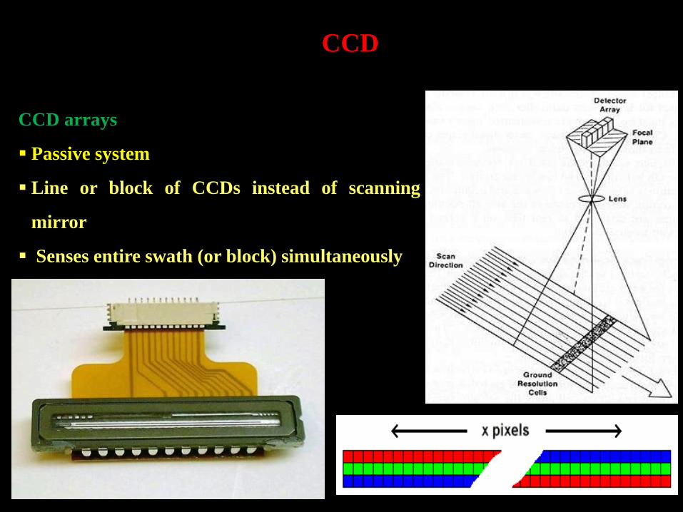
CCD arrays
Passive system
Line or block of CCDs instead of scanning
mirror
Senses entire swath (or block) simultaneously
CCD
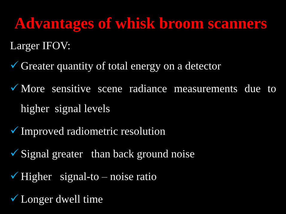
Advantages of whisk broom scanners
Larger IFOV:
Greater quantity of total energy on a detector
More sensitive scene radiance measurements due to
higher signal levels
Improved radiometric resolution
Signal greater than back ground noise
Higher signal-to – noise ratio
Longer dwell time
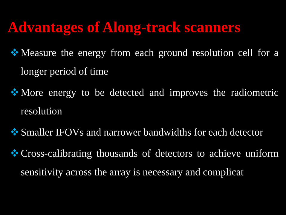
Advantages of Along-track scanners
Measure the energy from each ground resolution cell for a
longer period of time
More energy to be detected and improves the radiometric
resolution
Smaller IFOVs and narrower bandwidths for each detector
Cross-calibrating thousands of detectors to achieve uniform
sensitivity across the array is necessary and complicat
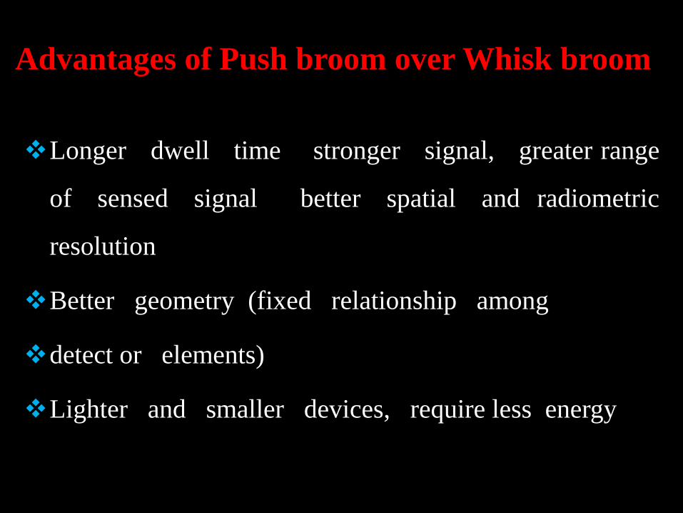
Advantages of Push broom over Whisk broom
Longer dwell time stronger signal, greater range
of sensed signal better spatial and radiometric
resolution
Better geometry (fixed relationship among
detect or elements)
Lighter and smaller devices, require less energy
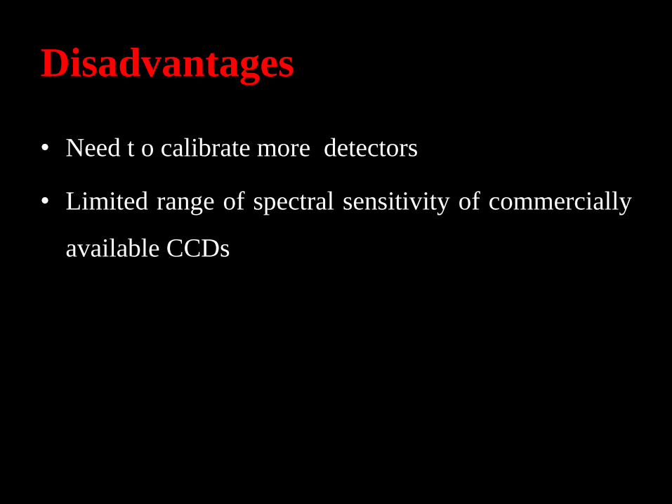
Disadvantages
• Need t o calibrate more detectors
• Limited range of spectral sensitivity of commercially
available CCDs
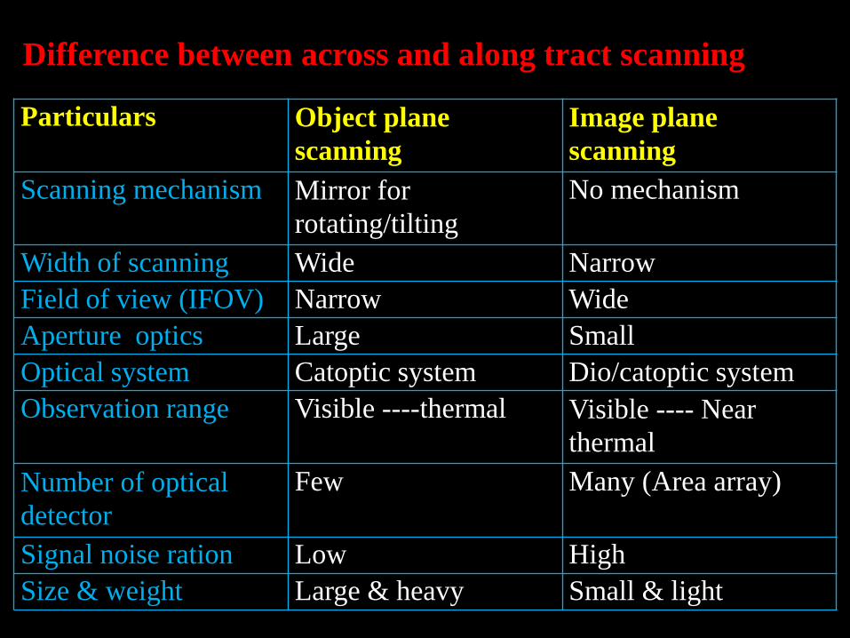
Difference between across and along tract scanning
Particulars Object plane
scanning
Image plane
scanning
Scanning mechanism Mirror for
rotating/tilting
No mechanism
Width of scanning Wide Narrow
Field of view (IFOV) Narrow Wide
Aperture optics Large Small
Optical system Catoptic system Dio/catoptic system
Observation range Visible ----thermal Visible ---- Near
thermal
Number of optical
detector
Few Many (Area array)
Signal noise ration Low High
Size & weight Large & heavy Small & light
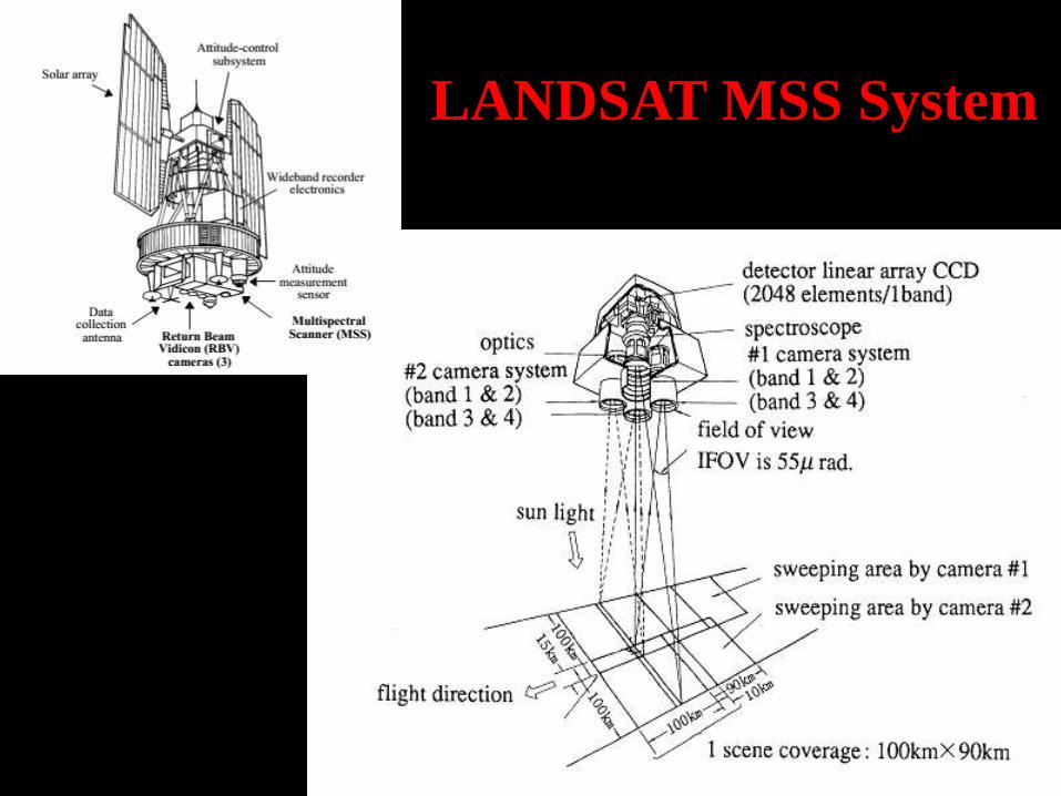
LANDSAT MSS SystemPush broom
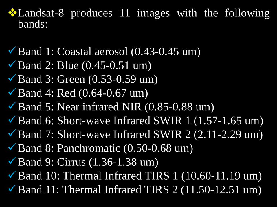
Landsat-8 produces 11 images with the followingbands:
Band 1: Coastal aerosol (0.43-0.45 um)
Band 2: Blue (0.45-0.51 um)
Band 3: Green (0.53-0.59 um)
Band 4: Red (0.64-0.67 um)
Band 5: Near infrared NIR (0.85-0.88 um)
Band 6: Short-wave Infrared SWIR 1 (1.57-1.65 um)
Band 7: Short-wave Infrared SWIR 2 (2.11-2.29 um)
Band 8: Panchromatic (0.50-0.68 um)
Band 9: Cirrus (1.36-1.38 um)
Band 10: Thermal Infrared TIRS 1 (10.60-11.19 um)
Band 11: Thermal Infrared TIRS 2 (11.50-12.51 um)
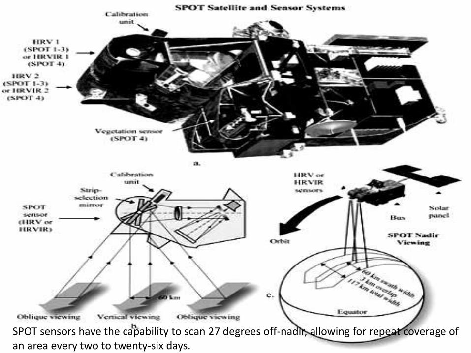
SPOT sensors have the capability to scan 27 degrees off-nadir, allowing for repeat coverage of an area every two to twenty-six days.
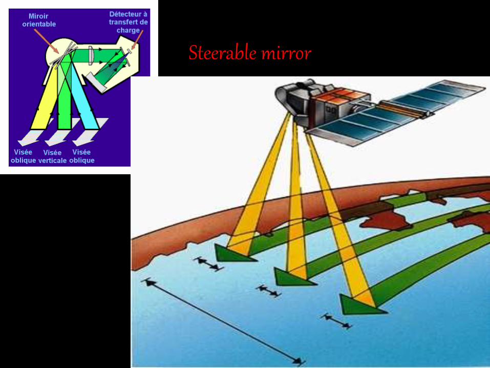
Steerable mirror
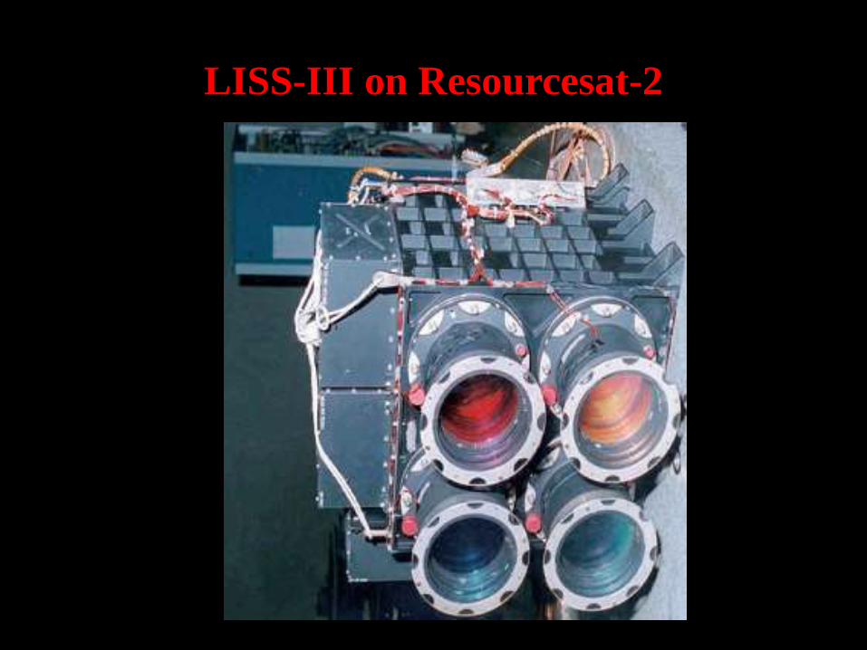
LISS-III on Resourcesat-2
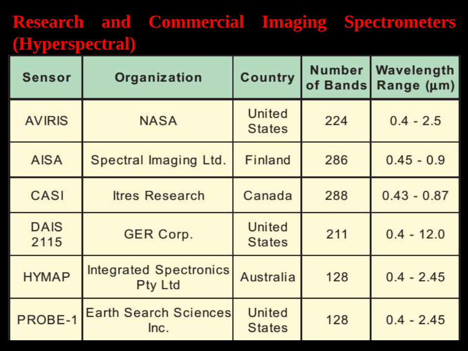
Research and Commercial Imaging Spectrometers
(Hyperspectral)
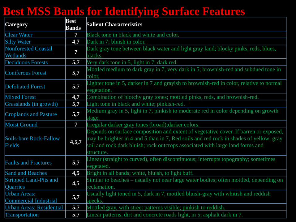
CategoryBest
BandsSalient Characteristics
Clear Water 7 Black tone in black and white and color.
Silty Water 4,7 Dark in 7; bluish in color.
Nonforested Coastal
Wetlands7
Dark gray tone between black water and light gray land; blocky pinks, reds, blues,
blacks.
Deciduous Forests 5,7 Very dark tone in 5, light in 7; dark red.
Coniferous Forest 5,7Mottled medium to dark gray in 7, very dark in 5; brownish-red and subdued tone in
color,
Defoliated Forest 5,7Lighter tone in 5, darker in 7 and grayish to brownish-red in color, relative to normal
vegetation.
Mixed Forest 4,7 Combination of blotchy gray tones; mottled pinks, reds, and brownish-red.
Grasslands (in growth) 5,7 Light tone in black and white; pinkish-red.
Croplands and Pasture 5,7Medium gray in 5, light in 7, pinkish to moderate red in color depending on growth
stage.
Moist Ground 7 Irregular darker gray tones (broad);darker colors.
Soils-bare Rock-Fallow
Fields4,5,7
Depends on surface composition and extent of vegetative cover. If barren or exposed,
may be brighter in 4 and 5 than in 7, Red soils and red rock in shades of yellow; gray
soil and rock dark bluish; rock outcrops associated with large land forms and
structure.
Faults and Fractures 5,7Linear (straight to curved), often discontinuous; interrupts topography; sometimes
vegetated.
Sand and Beaches 4,5 Bright in all bands; white, bluish, to light buff.
Stripped Land-Pits and
Quarries4,5
Similar to beaches – usually not near large water bodies; often mottled, depending on
reclamation.
Urban Areas:
Commercial Industrial5,7
Usually light toned in 5, dark in 7, mottled bluish-gray with whitish and reddish
specks.
Urban Areas: Residential 5,7 Mottled gray, with street patterns visible; pinkish to reddish.
Transportation 5,7 Linear patterns, dirt and concrete roads light, in 5; asphalt dark in 7.
Best MSS Bands for Identifying Surface Features
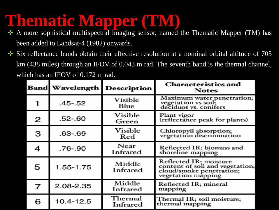
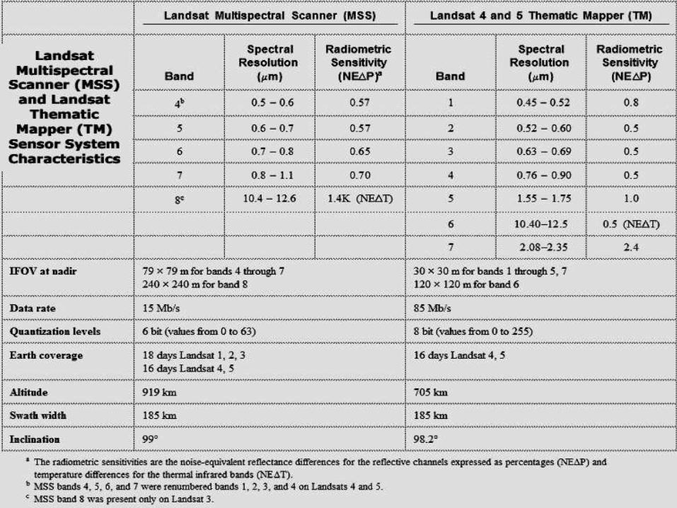
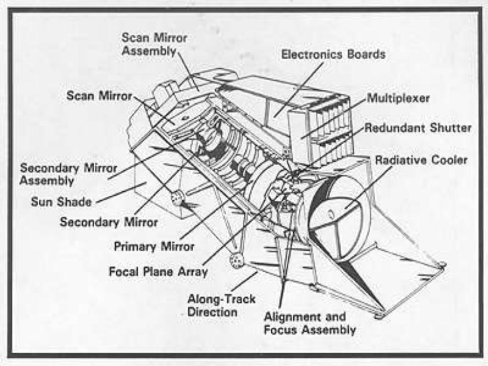
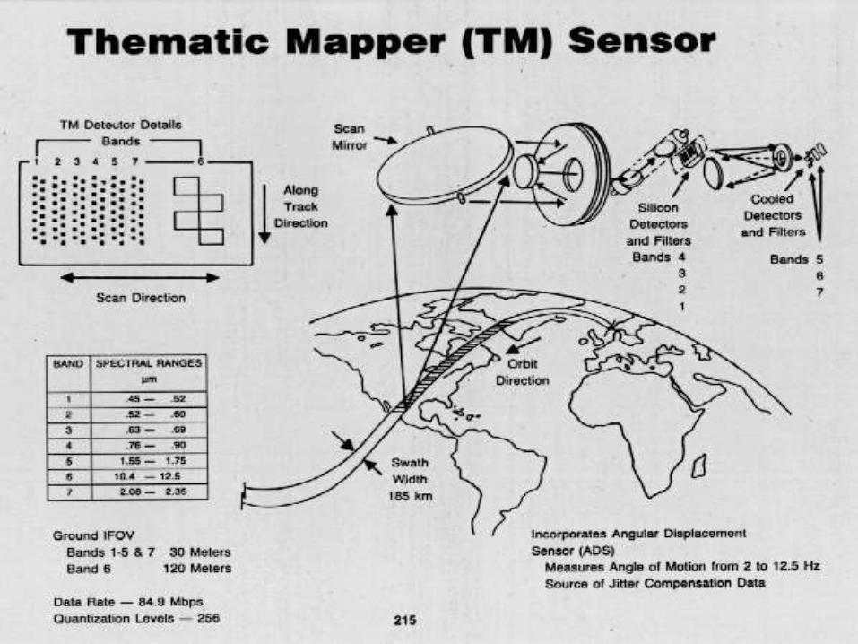
Thematic Mapper (TM) A more sophistical multispectral imaging sensor, named the Thematic Mapper (TM) has
been added to Landsat-4 (1982) onwards.
Six reflectance bands obtain their effective resolution at a nominal orbital altitude of 705
km (438 miles) through an IFOV of 0.043 m rad. The seventh band is the thermal channel,
which has an IFOV of 0.172 m rad.
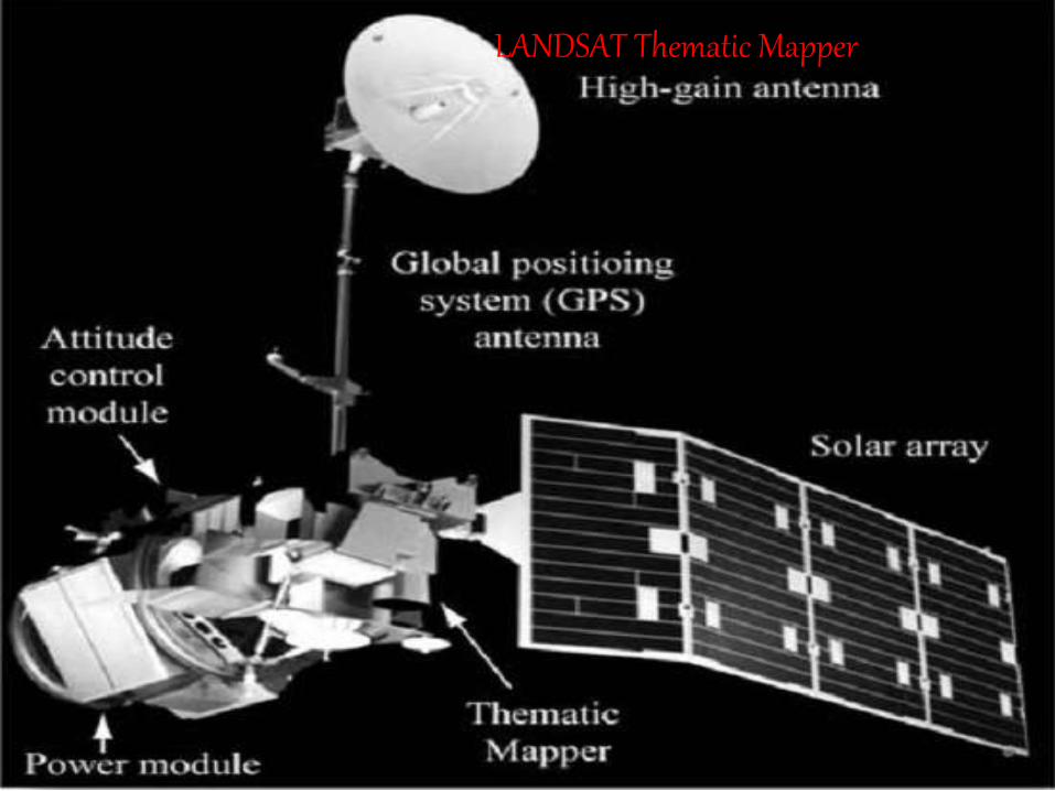
LANDSAT Thematic Mapper
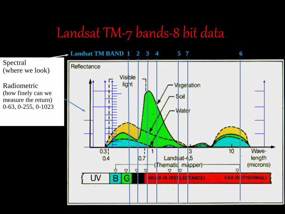
Landsat TM-7 bands-8 bit data
Spectral(where we look)
Radiometric(how finely can wemeasure the return)0-63, 0-255, 0-1023
Landsat TM BAND 1 2 3 4 5 7 6
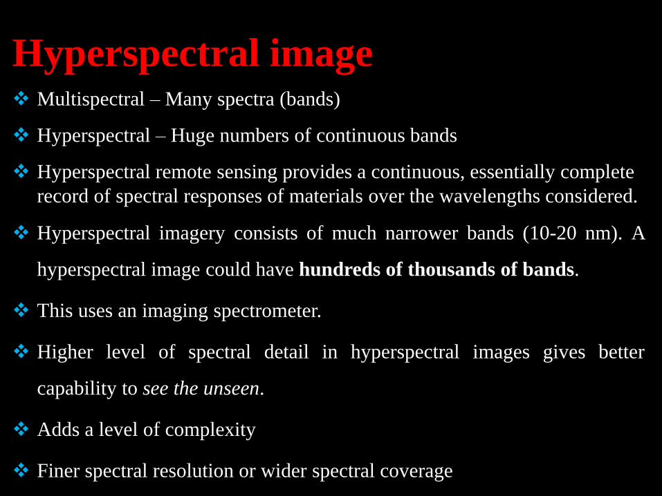
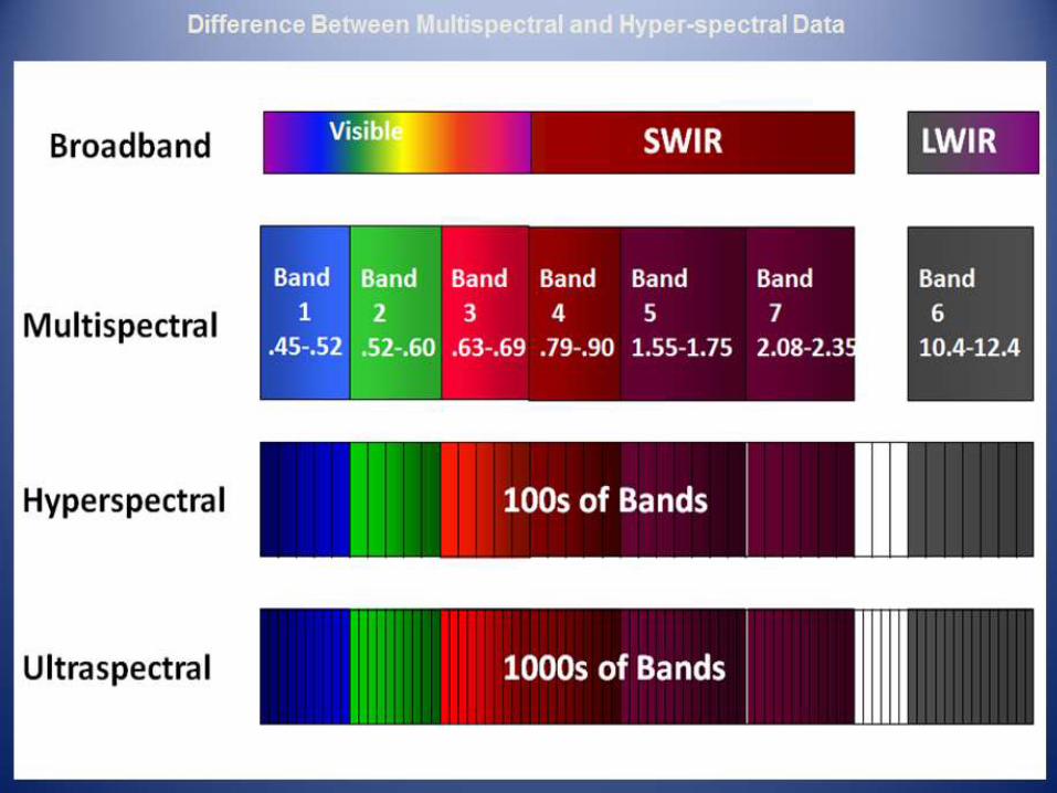
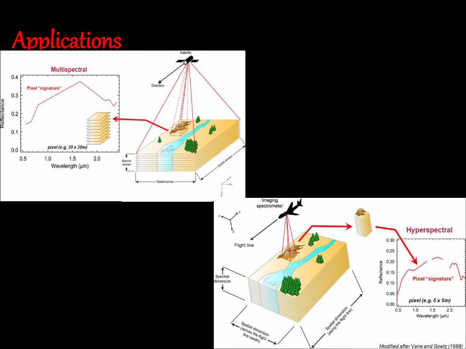
Hyperspectral image Multispectral – Many spectra (bands)
Hyperspectral – Huge numbers of continuous bands
Hyperspectral remote sensing provides a continuous, essentially complete
record of spectral responses of materials over the wavelengths considered.
Hyperspectral imagery consists of much narrower bands (10-20 nm). A
hyperspectral image could have hundreds of thousands of bands.
This uses an imaging spectrometer.
Higher level of spectral detail in hyperspectral images gives better
capability to see the unseen.
Adds a level of complexity
Finer spectral resolution or wider spectral coverage
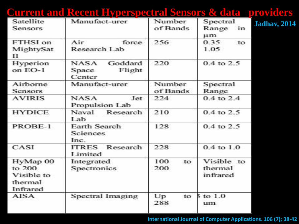
Current and Recent Hyperspectral Sensors & data providersJadhav, 2014
International Journal of Computer Applications. 106 (7); 38-42
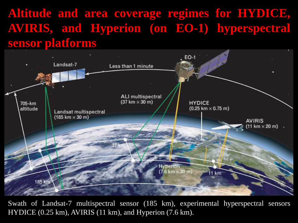
Altitude and area coverage regimes for HYDICE,
AVIRIS, and Hyperion (on EO-1) hyperspectral
sensor platforms
Swath of Landsat-7 multispectral sensor (185 km), experimental hyperspectral sensors
HYDICE (0.25 km), AVIRIS (11 km), and Hyperion (7.6 km).
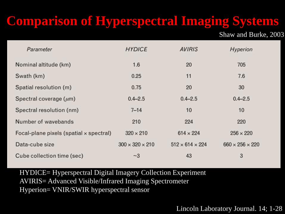
Comparison of Hyperspectral Imaging Systems
HYDICE= Hyperspectral Digital Imagery Collection Experiment
AVIRIS= Advanced Visible/Infrared Imaging Spectrometer
Hyperion= VNIR/SWIR hyperspectral sensor
Lincoln Laboratory Journal. 14; 1-28
Shaw and Burke, 2003
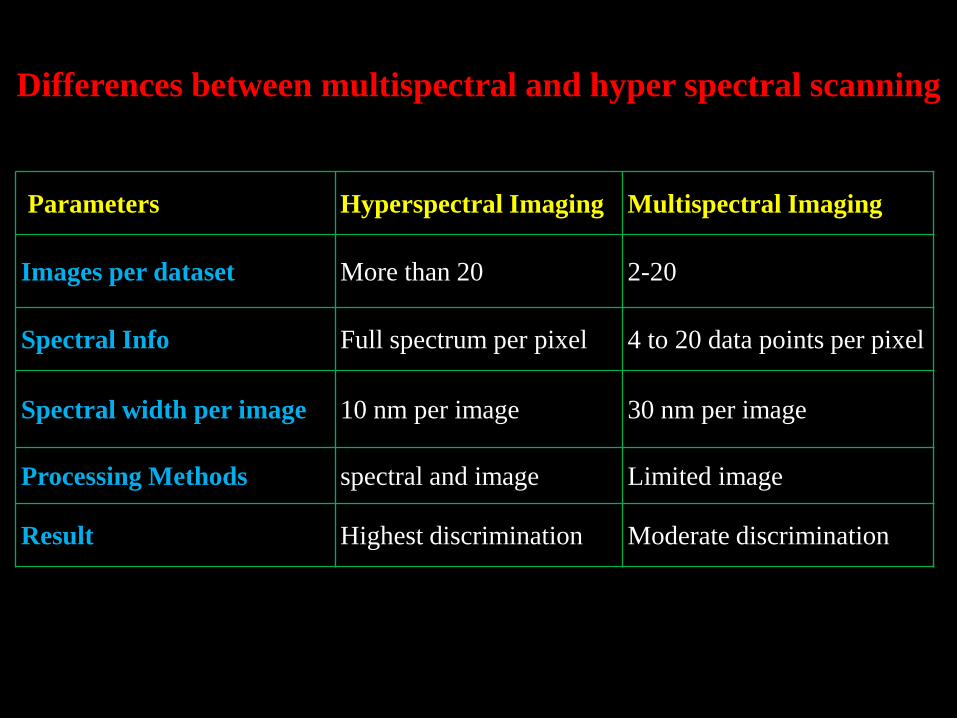
Differences between multispectral and hyper spectral scanning
Parameters Hyperspectral Imaging Multispectral Imaging
Images per dataset More than 20 2-20
Spectral Info Full spectrum per pixel 4 to 20 data points per pixel
Spectral width per image 10 nm per image 30 nm per image
Processing Methods spectral and image Limited image
Result Highest discrimination Moderate discrimination
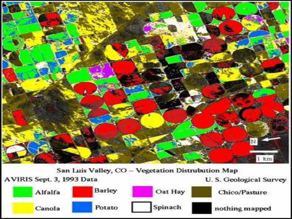
Applications
Spectral Signatures of 4 Materials
Band 1 = 0.55 um Band 2 = 0.85 um
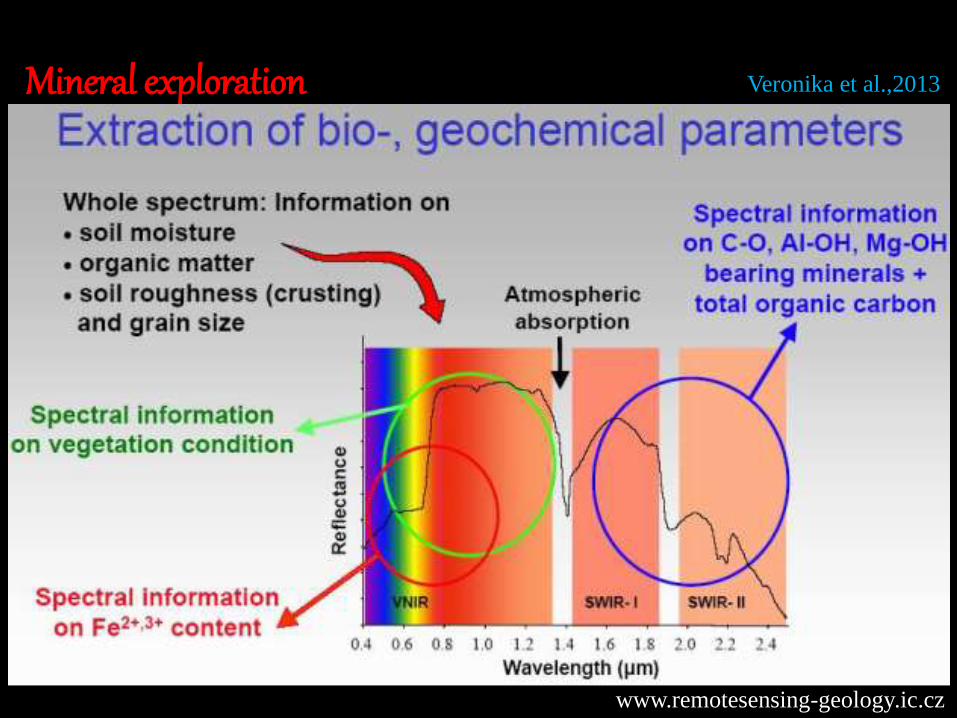
Mineral exploration
www.remotesensing-geology.ic.cz
Veronika et al.,2013
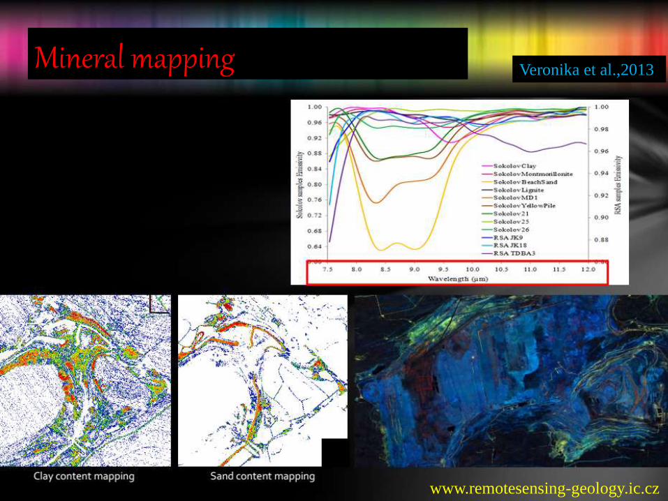
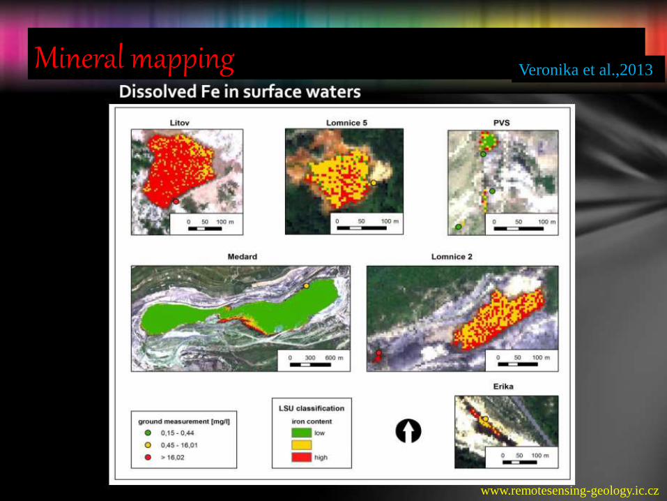
Mineral mapping
www.remotesensing-geology.ic.cz
Veronika et al.,2013
Mineral mapping
www.remotesensing-geology.ic.cz
Veronika et al.,2013
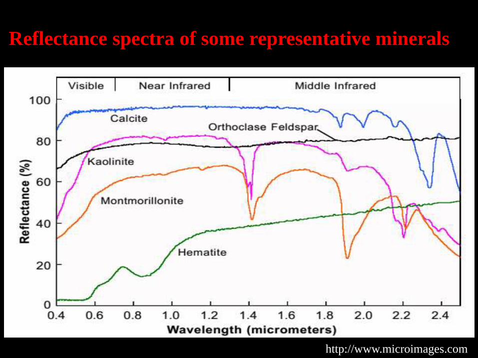
Reflectance spectra of some representative minerals
http://www.microimages.com
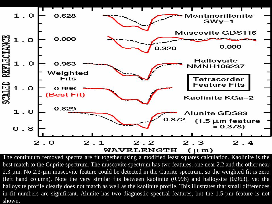
The continuum removed spectra are fit together using a modified least squares calculation. Kaolinite is the
best match to the Cuprite spectrum. The muscovite spectrum has two features, one near 2.2 and the other near
2.3 µm. No 2.3-µm muscovite feature could be detected in the Cuprite spectrum, so the weighted fit is zero
(left hand column). Note the very similar fits between kaolinite (0.996) and halloysite (0.963), yet the
halloysite profile clearly does not match as well as the kaolinite profile. This illustrates that small differences
in fit numbers are significant. Alunite has two diagnostic spectral features, but the 1.5-µm feature is not
shown.
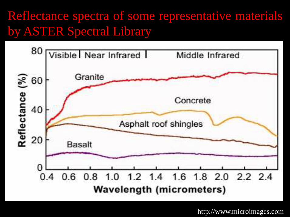
Reflectance spectra of some representative materials
by ASTER Spectral Library
http://www.microimages.com
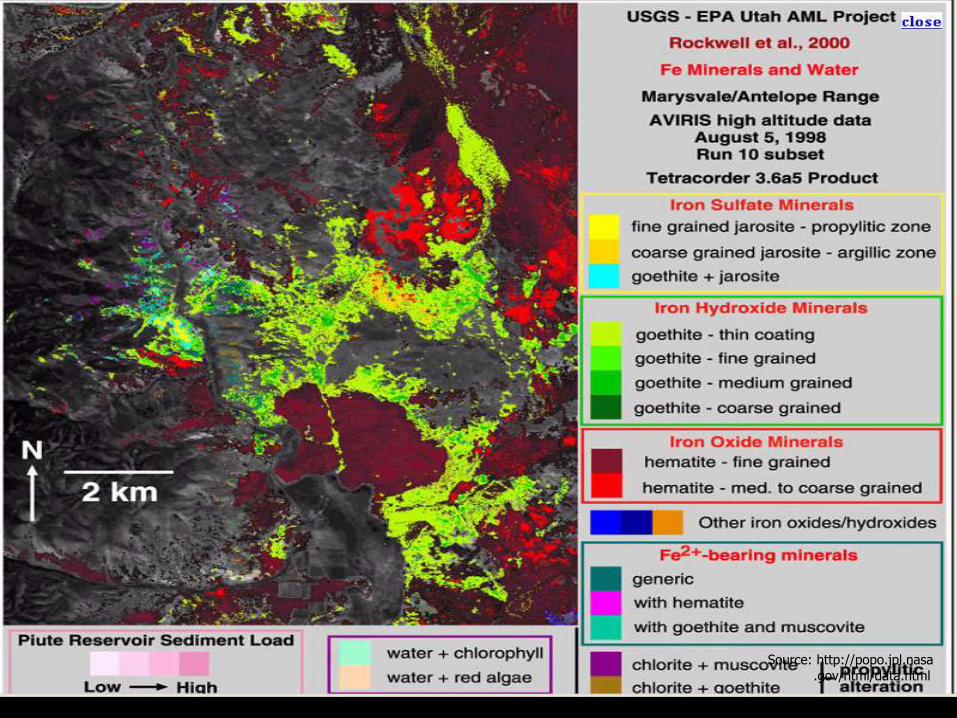
Source: http://popo.jpl.nasa.gov/html/data.html
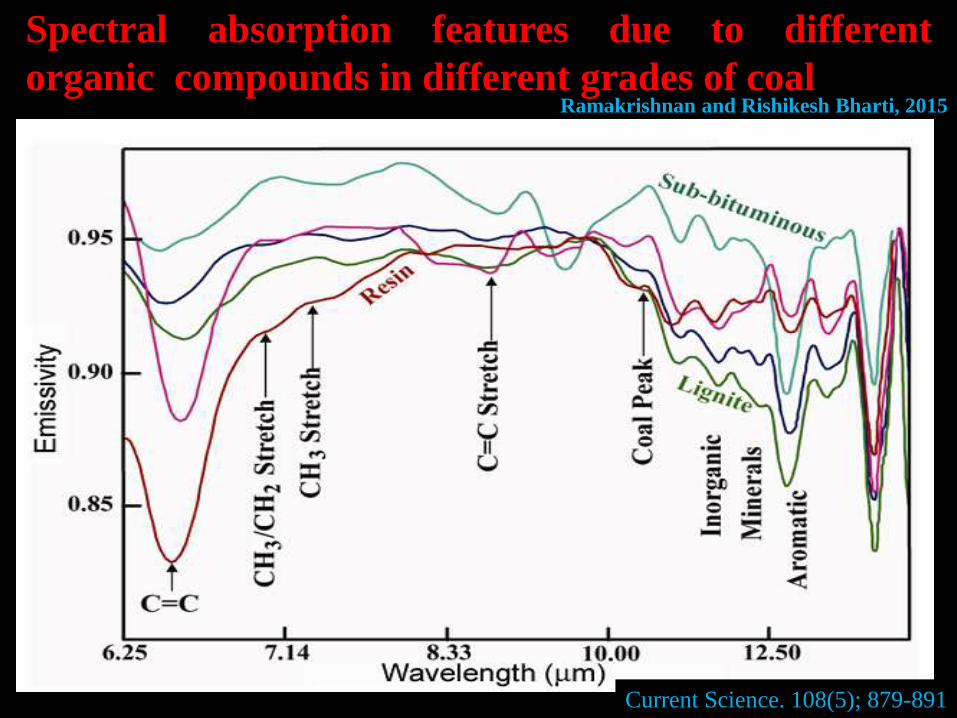
Spectral absorption features due to different
organic compounds in different grades of coalRamakrishnan and Rishikesh Bharti, 2015
Current Science. 108(5); 879-891
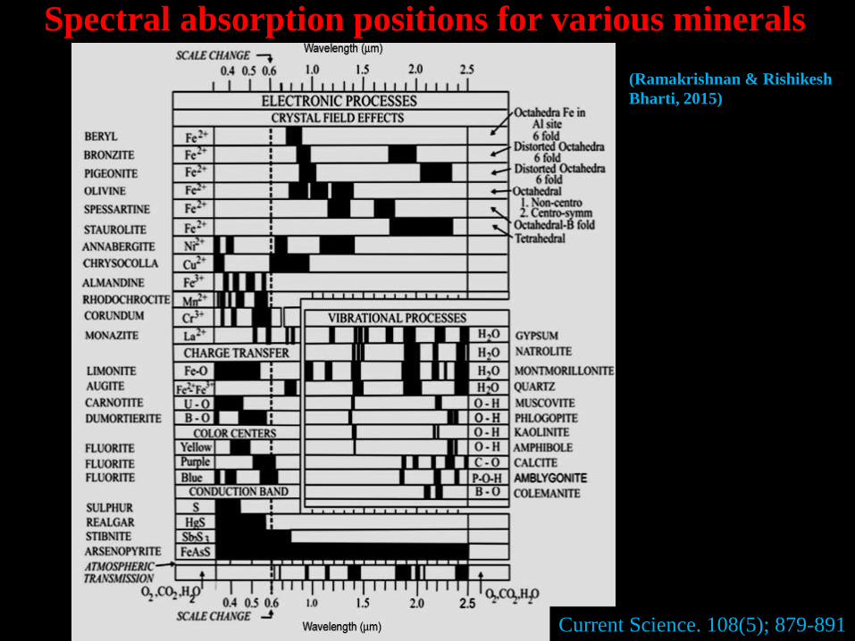
Spectral absorption positions for various minerals
(Ramakrishnan & Rishikesh
Bharti, 2015)
Current Science. 108(5); 879-891
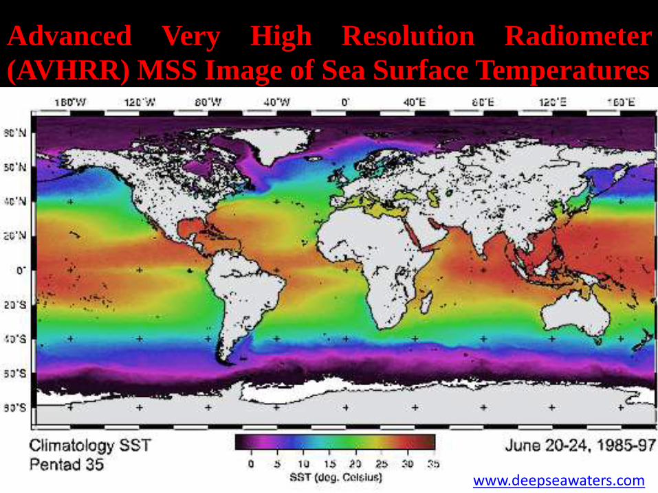
Advanced Very High Resolution Radiometer
(AVHRR) MSS Image of Sea Surface Temperatures
www.deepseawaters.com
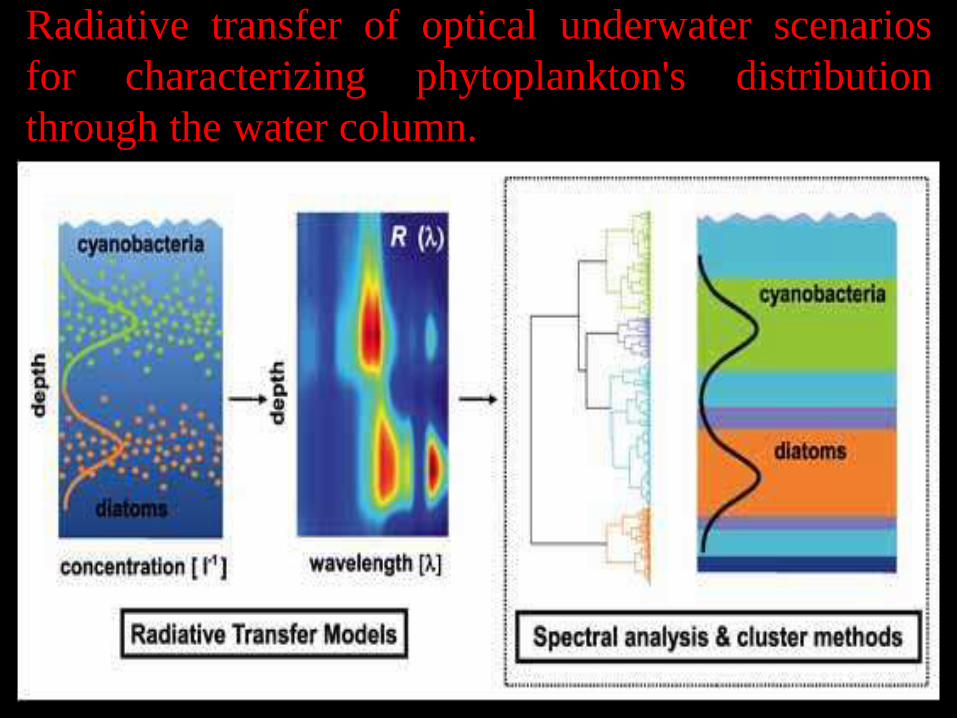
Radiative transfer of optical underwater scenarios
for characterizing phytoplankton's distribution
through the water column. dzyr rsezy TYWTWETEf
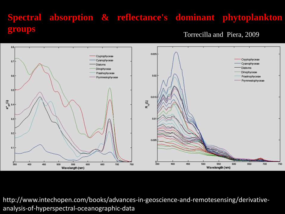
Spectral absorption & reflectance's dominant phytoplankton
groupsTorrecilla and Piera, 2009
http://www.intechopen.com/books/advances-in-geoscience-and-remotesensing/derivative-analysis-of-hyperspectral-oceanographic-data
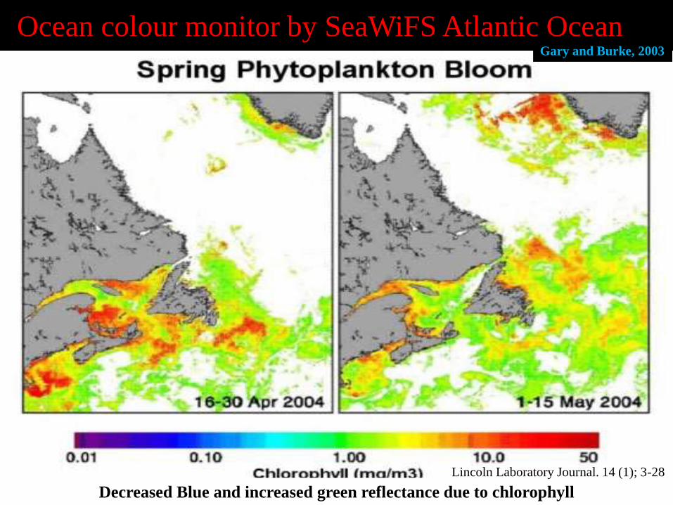
Ocean colour monitor by SeaWiFS Atlantic Ocean
Decreased Blue and increased green reflectance due to chlorophyll
Gary and Burke, 2003
Lincoln Laboratory Journal. 14 (1); 3-28
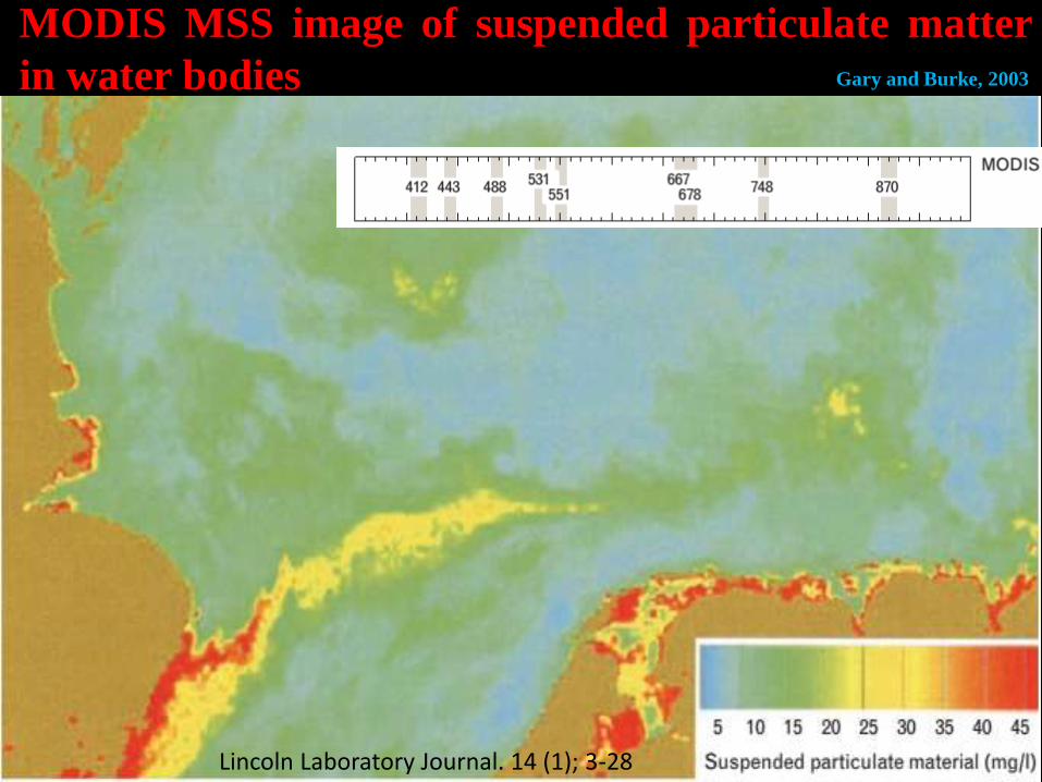
MODIS MSS image of suspended particulate matter
in water bodies Gary and Burke, 2003
Lincoln Laboratory Journal. 14 (1); 3-28
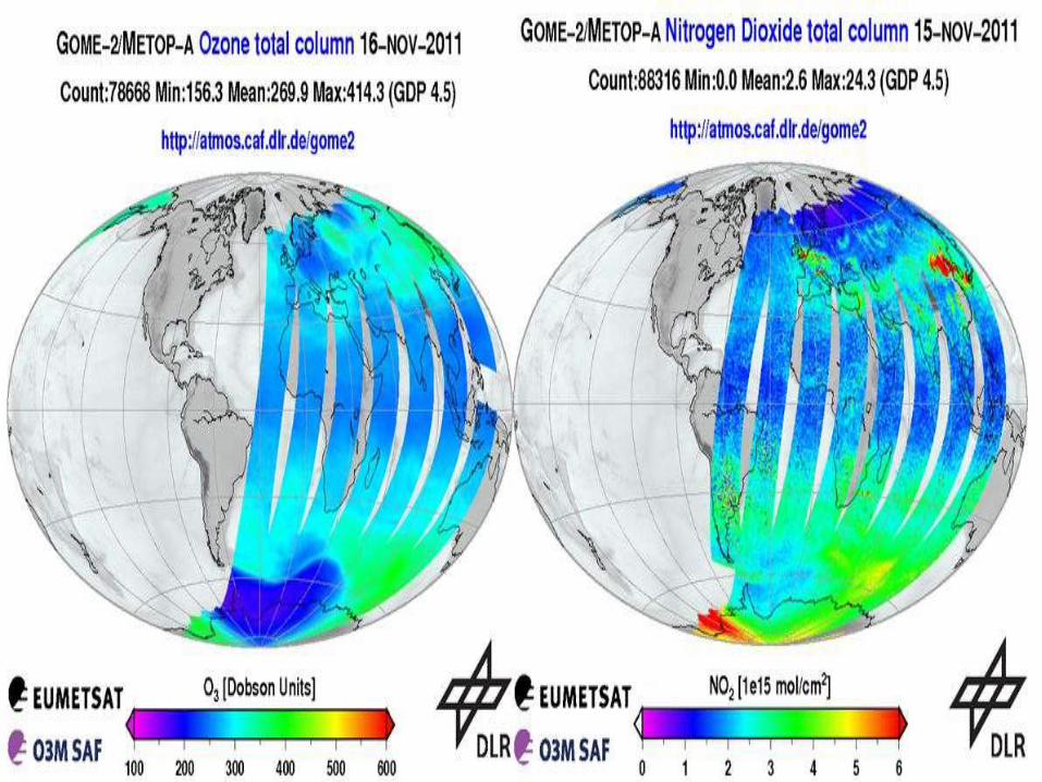
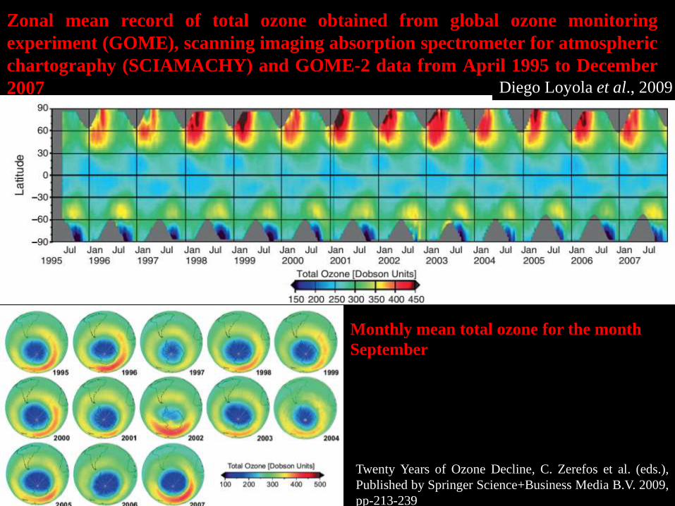
Zonal mean record of total ozone obtained from global ozone monitoring
experiment (GOME), scanning imaging absorption spectrometer for atmospheric
chartography (SCIAMACHY) and GOME-2 data from April 1995 to December
2007
Monthly mean total ozone for the month
September
Diego Loyola et al., 2009
Twenty Years of Ozone Decline, C. Zerefos et al. (eds.),
Published by Springer Science+Business Media B.V. 2009,
pp-213-239
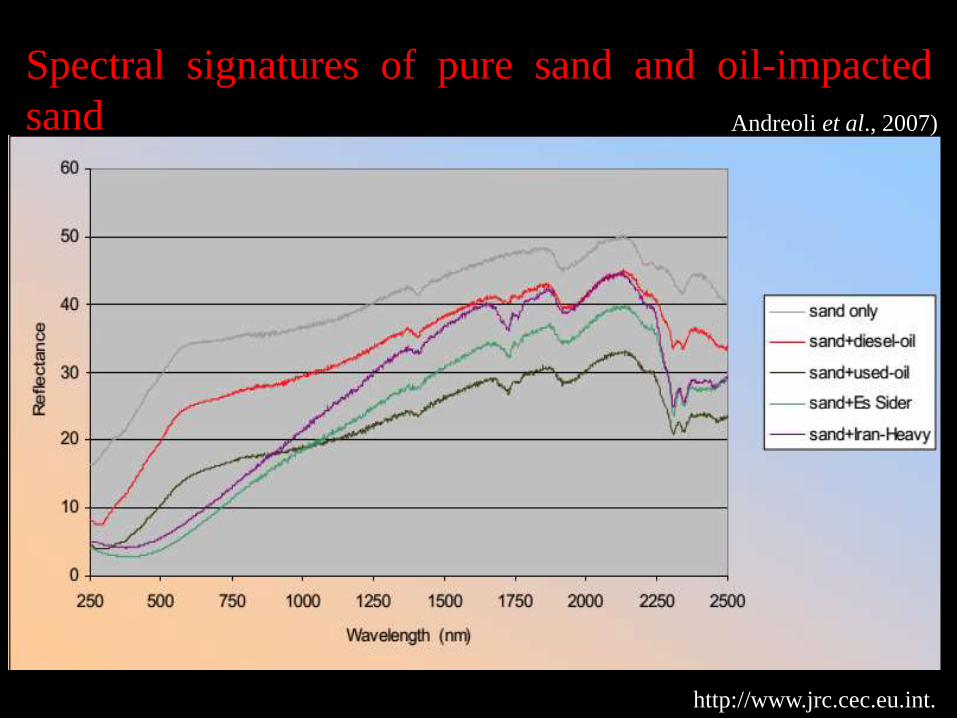
Spectral signatures of pure sand and oil-impacted
sand Andreoli et al., 2007)
http://www.jrc.cec.eu.int.http://www.jrc.cec.eu.int.http://www.jrc.cec.eu.int.
http://www.jrc.cec.eu.int.
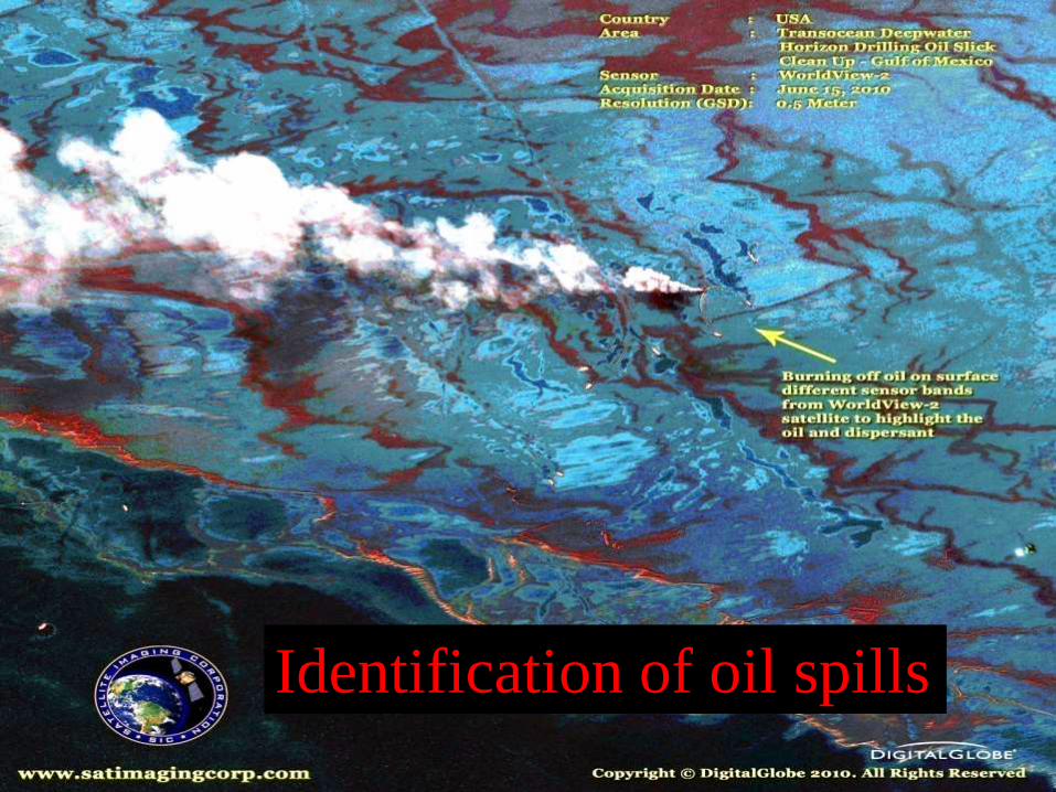
Identification of oil spills
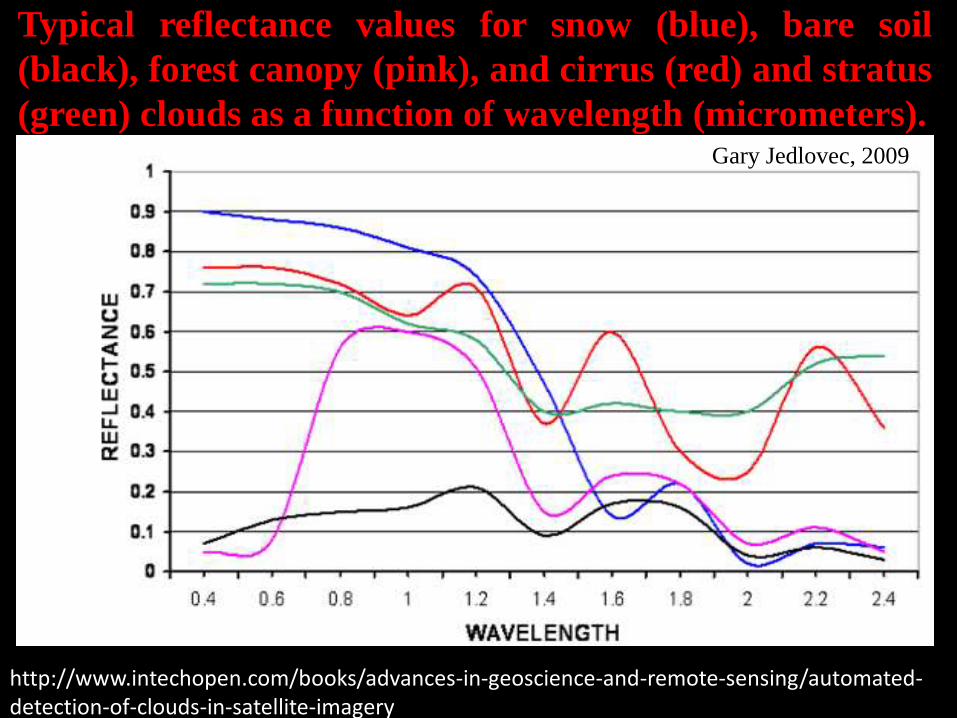
Typical reflectance values for snow (blue), bare soil
(black), forest canopy (pink), and cirrus (red) and stratus
(green) clouds as a function of wavelength (micrometers).Gary Jedlovec, 2009
http://www.intechopen.com/books/advances-in-geoscience-and-remote-sensing/automated-detection-of-clouds-in-satellite-imagery
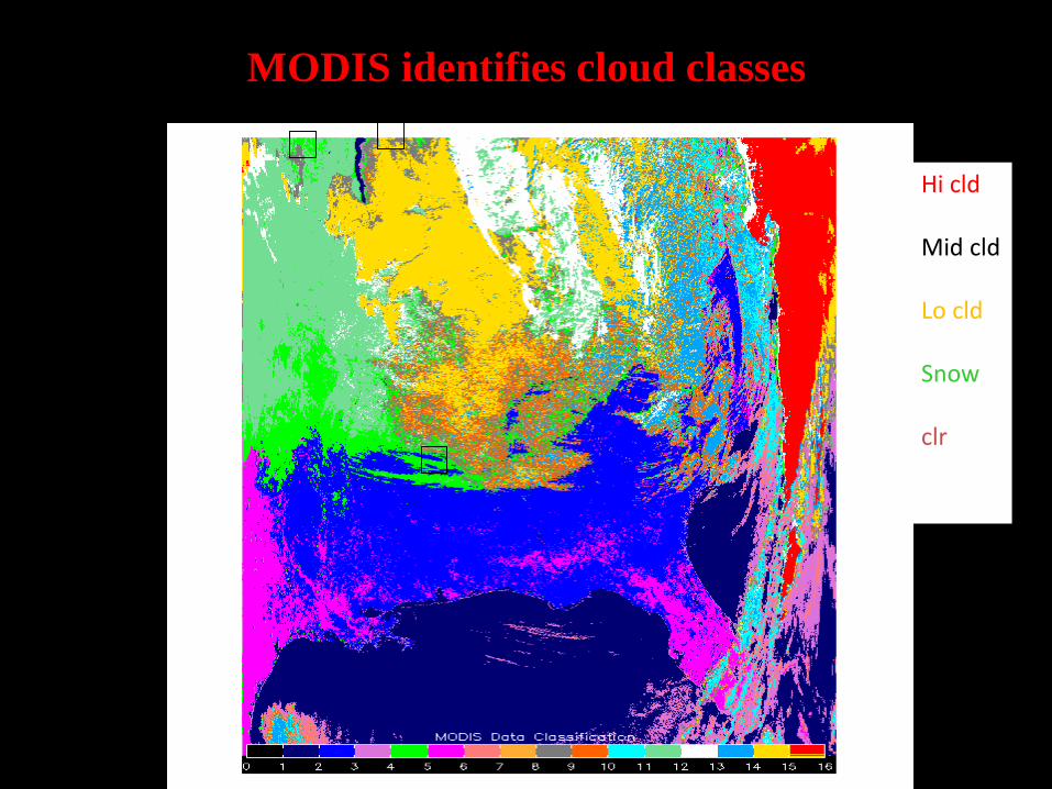
MODIS identifies cloud classes
Hi cld
Mid cld
Lo cld
Snow
clr
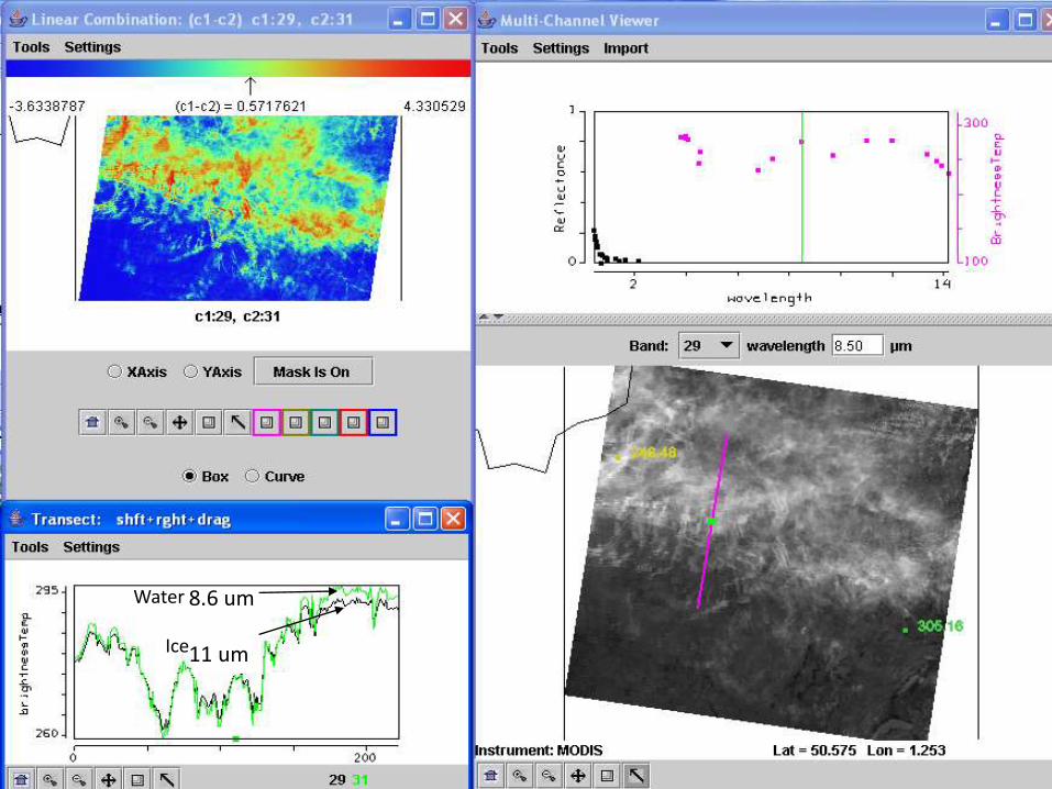
8.6 um
11 um
Water
Ice
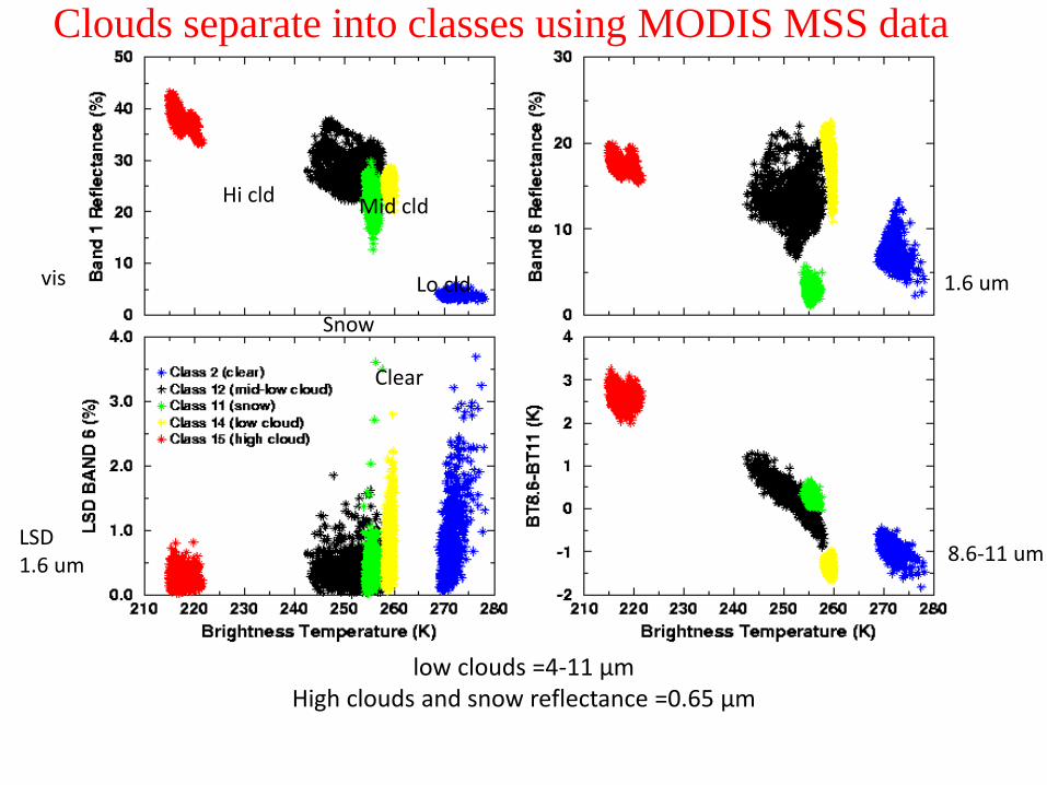
Clouds separate into classes using MODIS MSS data
Hi cld
Snow
Lo cld
Clear
Mid cld
11 um 11 um
vis
LSD 1.6 um
1.6 um
8.6-11 um
low clouds =4-11 μmHigh clouds and snow reflectance =0.65 μm
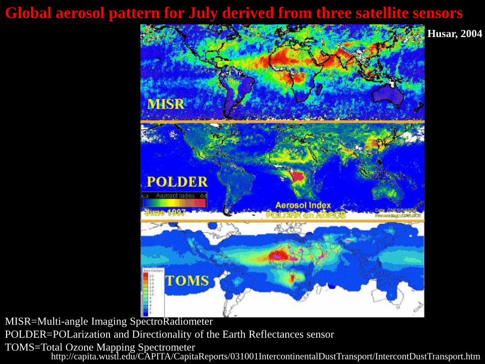
Global aerosol pattern for July derived from three satellite sensors
MISR=Multi-angle Imaging SpectroRadiometer
POLDER=POLarization and Directionality of the Earth Reflectances sensor
TOMS=Total Ozone Mapping Spectrometer
Husar, 2004
http://capita.wustl.edu/CAPITA/CapitaReports/031001IntercontinentalDustTransport/IntercontDustTransport.htm
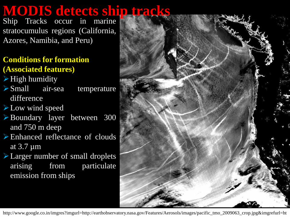
Ship Tracks occur in marine
stratocumulus regions (California,
Azores, Namibia, and Peru)
Conditions for formation
(Associated features)
High humidity
Small air-sea temperature
difference
Low wind speed
Boundary layer between 300
and 750 m deep
Enhanced reflectance of clouds
at 3.7 µm
Larger number of small droplets
arising from particulate
emission from ships
MODIS detects ship tracks
http://www.google.co.in/imgres?imgurl=http://earthobservatory.nasa.gov/Features/Aerosols/images/pacific_tmo_2009063_crop.jpg&imgrefurl=ht
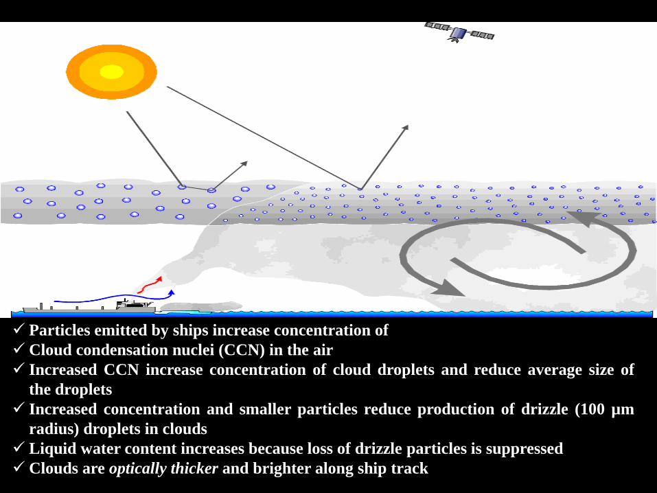
Particles emitted by ships increase concentration of
Cloud condensation nuclei (CCN) in the air
Increased CCN increase concentration of cloud droplets and reduce average size of
the droplets
Increased concentration and smaller particles reduce production of drizzle (100 µm
radius) droplets in clouds
Liquid water content increases because loss of drizzle particles is suppressed
Clouds are optically thicker and brighter along ship track
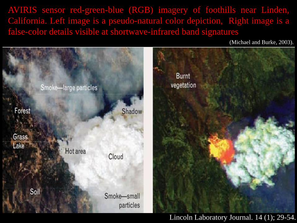
AVIRIS sensor red-green-blue (RGB) imagery of foothills near Linden,
California. Left image is a pseudo-natural color depiction, Right image is a
false-color details visible at shortwave-infrared band signatures(Michael and Burke, 2003).
Lincoln Laboratory Journal. 14 (1); 29-54.
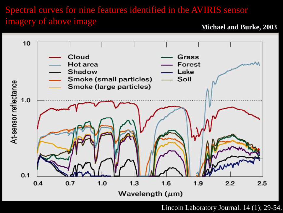
Spectral curves for nine features identified in the AVIRIS sensor
imagery of above imageMichael and Burke, 2003
Lincoln Laboratory Journal. 14 (1); 29-54.
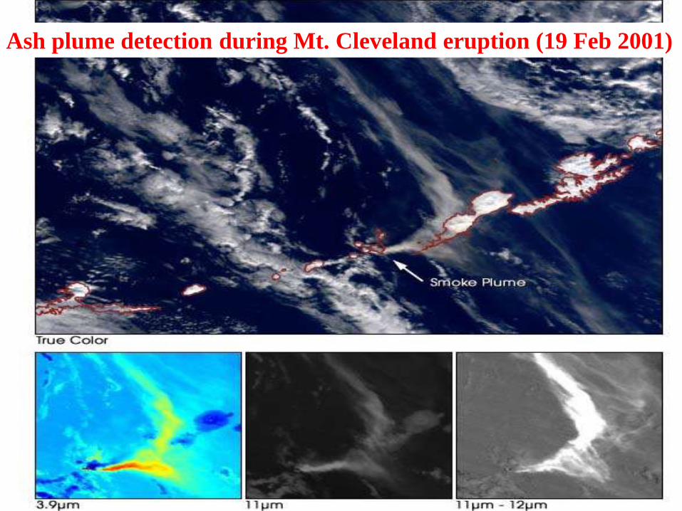
Ash plume detection during Mt. Cleveland eruption (19 Feb 2001)
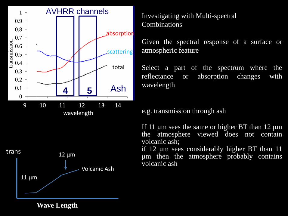
Investigating with Multi-spectral
Combinations
Given the spectral response of a surface or
atmospheric feature
Select a part of the spectrum where the
reflectance or absorption changes with
wavelength
e.g. transmission through ash
If 11 μm sees the same or higher BT than 12 μmthe atmosphere viewed does not containvolcanic ash;if 12 μm sees considerably higher BT than 11μm then the atmosphere probably containsvolcanic ash
trans
Wave Length
11 μm
12 μm
Volcanic Ash
3
0.86
0.88
0.9
0.92
0.94
0.96
0.98
1
7 8 9 10 11 12 13 14
wavelength (m)
transmission (total)transmission (scattering)transmission (absorption)
0
0.1
0.2
0.3
0.4
0.5
0.6
0.7
0.8
0.9
1
7 8 9 10 11 12 13 14
wavelength (m)
transmission (total)transmission (scattering)transmission (absorption)
4 50
0.1
0.2
0.3
0.4
0.5
0.6
0.7
0.8
0.9
1
7 8 9 10 11 12 13 14
tran
smis
sion
9
0
0.1
0.2
0.3
0.4
0.5
0.6
0.7
0.8
0.9
1
7 8 9 10 11 12 13 14
tran
smis
sion
9
4 5
T10.8 - T12.0 > 0 water & ice
T10.8 - T12.0 < 0 volcanic ash
Source: Dr. M. Watson, Michigan Technical University
Ice Ash
0
0.1
0.2
0.3
0.4
0.5
0.6
0.7
0.8
0.9
1
7 8 9 10 11 12 13 14
transmission (total)transmission (scattering)transmission (absorption)
Wavelength (m) Wavelength (m)
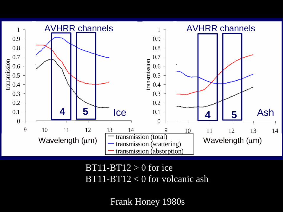
Spectral features of ice and ash in
the 10-13 m waveband
AVHRR channels AVHRR channels
ET-ODRRGOS, Oxford, UK, 1-5 July
2002
absorption
scattering
total
9 10 11 12 13 14wavelength
3
0.86
0.88
0.9
0.92
0.94
0.96
0.98
1
7 8 9 10 11 12 13 14
wavelength (m)
transmission (total)transmission (scattering)transmission (absorption)
0
0.1
0.2
0.3
0.4
0.5
0.6
0.7
0.8
0.9
1
7 8 9 10 11 12 13 14
wavelength (m)
transmission (total)transmission (scattering)transmission (absorption)
4 50
0.1
0.2
0.3
0.4
0.5
0.6
0.7
0.8
0.9
1
7 8 9 10 11 12 13 14
tran
smis
sion
9
0
0.1
0.2
0.3
0.4
0.5
0.6
0.7
0.8
0.9
1
7 8 9 10 11 12 13 14
tran
smis
sion
9
4 5
T10.8 - T12.0 > 0 water & ice
T10.8 - T12.0 < 0 volcanic ash
Source: Dr. M. Watson, Michigan Technical University
Ice Ash
0
0.1
0.2
0.3
0.4
0.5
0.6
0.7
0.8
0.9
1
7 8 9 10 11 12 13 14
transmission (total)transmission (scattering)transmission (absorption)
Wavelength (m) Wavelength (m)
Spectral features of ice and ash in
the 10-13 m waveband
AVHRR channels AVHRR channels
ET-ODRRGOS, Oxford, UK, 1-5 July
2002
BT11-BT12 > 0 for ice
BT11-BT12 < 0 for volcanic ash
Frank Honey 1980s
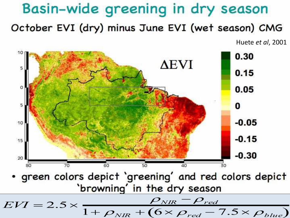
Huete et al, 2001
EVI 2.5NIR red
1 NIR 6 red 7.5 blue
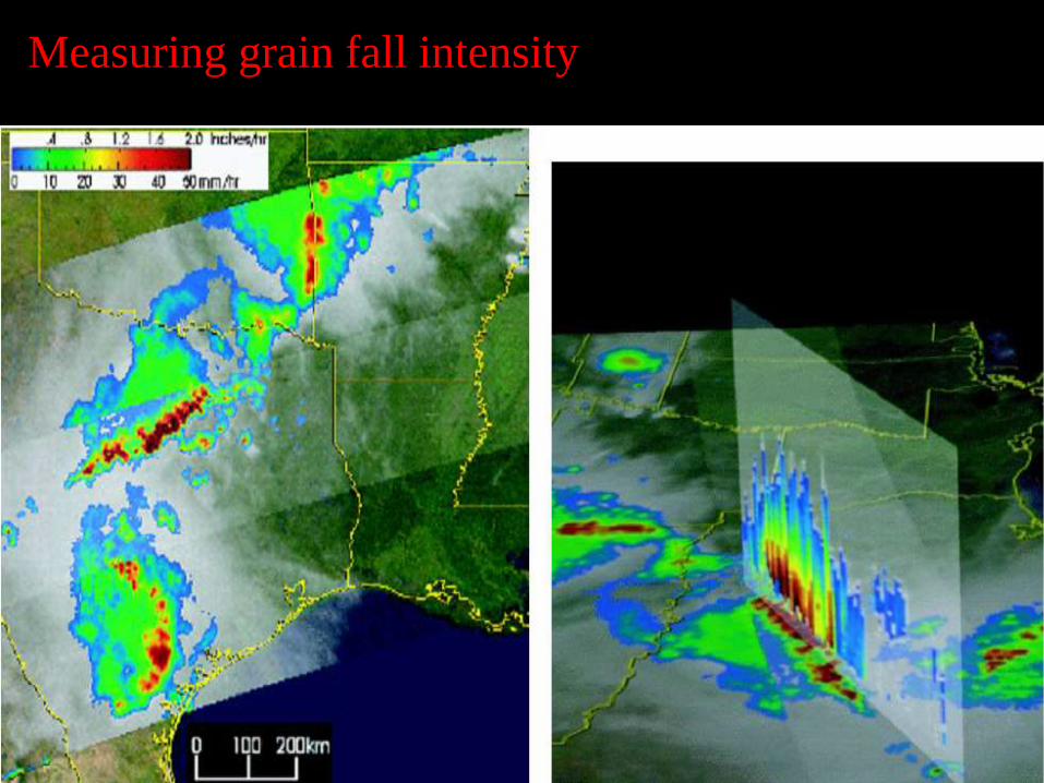
Measuring grain fall intensity
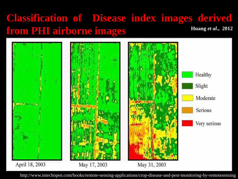
Classification of Disease index images derived
from PHI airborne images Huang et al., 2012
http://www.intechopen.com/books/remote-sensing-applications/crop-disease-and-pest-monitoring-by-remotesensing
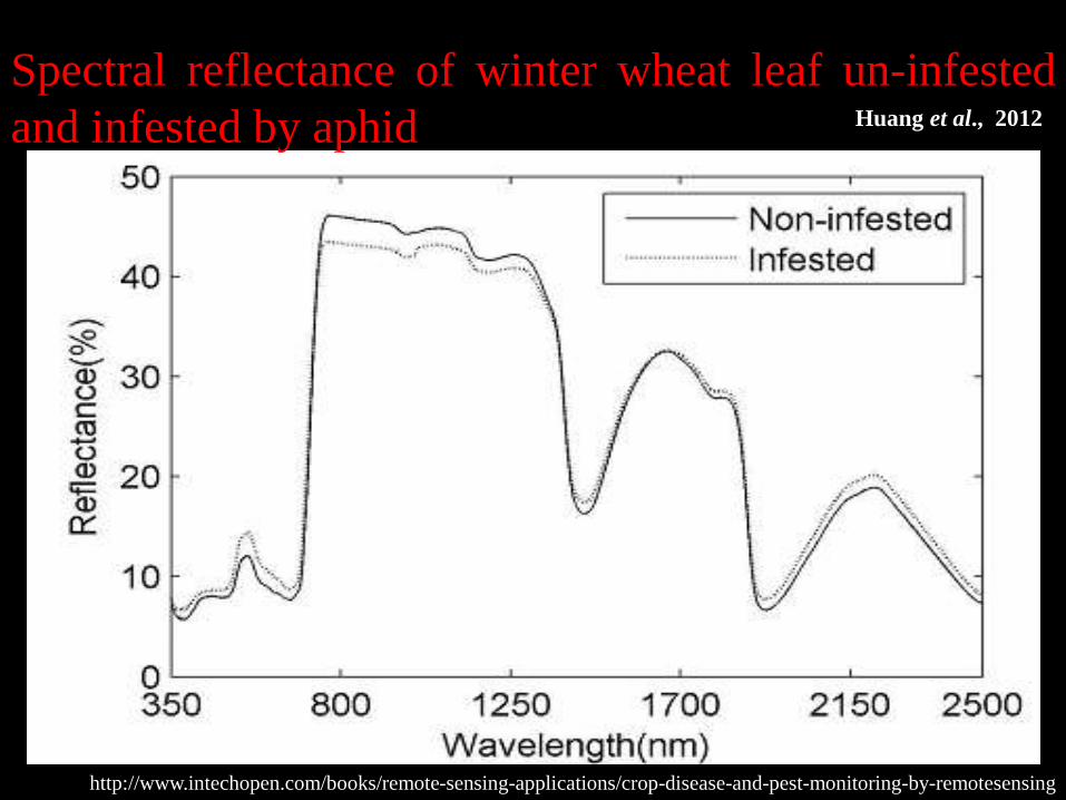
Spectral reflectance of winter wheat leaf un-infested
and infested by aphid Huang et al., 2012
http://www.intechopen.com/books/remote-sensing-applications/crop-disease-and-pest-monitoring-by-remotesensing
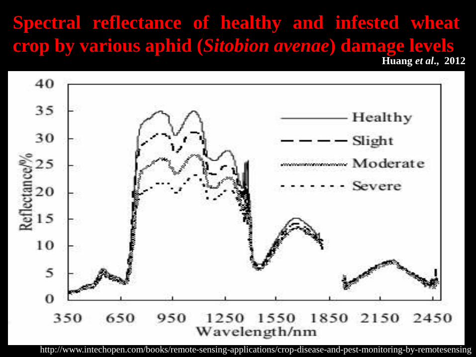
Spectral reflectance of healthy and infested wheat
crop by various aphid (Sitobion avenae) damage levelsHuang et al., 2012
http://www.intechopen.com/books/remote-sensing-applications/crop-disease-and-pest-monitoring-by-remotesensing
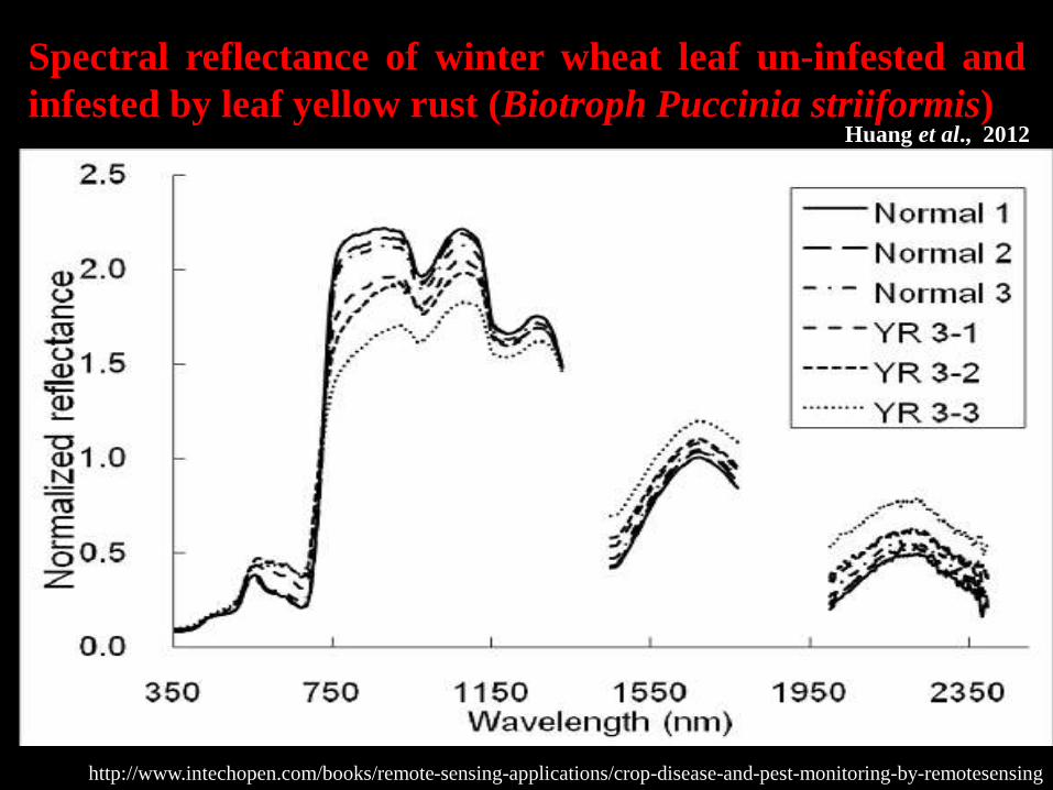
Spectral reflectance of winter wheat leaf un-infested and
infested by leaf yellow rust (Biotroph Puccinia striiformis)Huang et al., 2012
http://www.intechopen.com/books/remote-sensing-applications/crop-disease-and-pest-monitoring-by-remotesensing
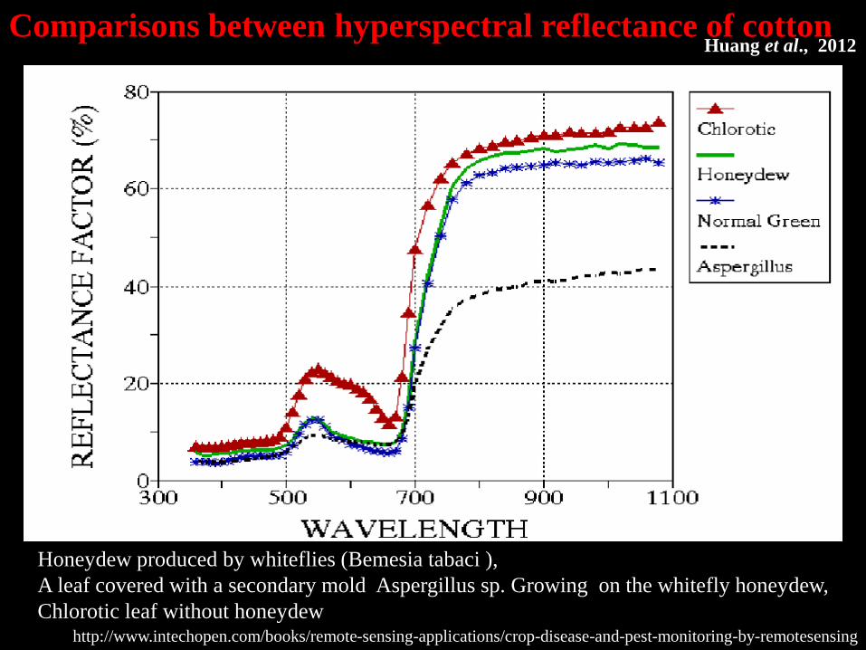
Comparisons between hyperspectral reflectance of cotton
Honeydew produced by whiteflies (Bemesia tabaci ),
A leaf covered with a secondary mold Aspergillus sp. Growing on the whitefly honeydew,
Chlorotic leaf without honeydew
Huang et al., 2012
http://www.intechopen.com/books/remote-sensing-applications/crop-disease-and-pest-monitoring-by-remotesensing
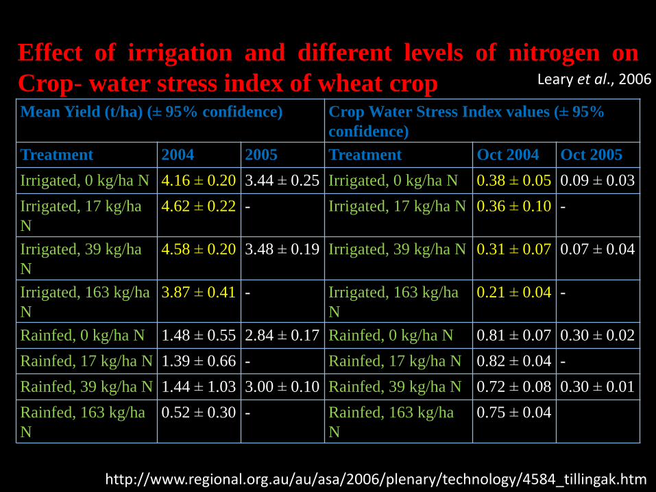
Mean Yield (t/ha) (± 95% confidence) Crop Water Stress Index values (± 95%
confidence)
Treatment 2004 2005 Treatment Oct 2004 Oct 2005
Irrigated, 0 kg/ha N 4.16 ± 0.20 3.44 ± 0.25 Irrigated, 0 kg/ha N 0.38 ± 0.05 0.09 ± 0.03
Irrigated, 17 kg/ha
N
4.62 ± 0.22 - Irrigated, 17 kg/ha N 0.36 ± 0.10 -
Irrigated, 39 kg/ha
N
4.58 ± 0.20 3.48 ± 0.19 Irrigated, 39 kg/ha N 0.31 ± 0.07 0.07 ± 0.04
Irrigated, 163 kg/ha
N
3.87 ± 0.41 - Irrigated, 163 kg/ha
N
0.21 ± 0.04 -
Rainfed, 0 kg/ha N 1.48 ± 0.55 2.84 ± 0.17 Rainfed, 0 kg/ha N 0.81 ± 0.07 0.30 ± 0.02
Rainfed, 17 kg/ha N 1.39 ± 0.66 - Rainfed, 17 kg/ha N 0.82 ± 0.04 -
Rainfed, 39 kg/ha N 1.44 ± 1.03 3.00 ± 0.10 Rainfed, 39 kg/ha N 0.72 ± 0.08 0.30 ± 0.01
Rainfed, 163 kg/ha
N
0.52 ± 0.30 - Rainfed, 163 kg/ha
N
0.75 ± 0.04
Effect of irrigation and different levels of nitrogen on
Crop- water stress index of wheat crop Leary et al., 2006
http://www.regional.org.au/au/asa/2006/plenary/technology/4584_tillingak.htm


