

MULTIROUTING BEHAVIOR IN STREAM CONTROL TRANSMISSION
PROTOCOL
By
JAGDISH KUMAR GOPALAKRISHNAN
A THESIS PRESENTED TO THE GRADUATE SCHOOL OF THE UNIVERSITY OF FLORIDA IN PARTIAL FULFILLMENT
OF THE REQUIREMENTS FOR THE DEGREE OF MASTER OF SCIENCE
UNIVERSITY OF FLORIDA
2003

Copyright 2003
by
Jagdish Kumar Gopalakrishnan

Dedicated to my family

ACKNOWLEDGMENTS
First and foremost, I would like to express my deepest reverence, gratitude and
appreciation to Dr. Richard Newman, the chair of my committee. This thesis would not
have been possible if it were not for his continuous direction and encouragement at each
phase of this thesis. I would also like to thank Dr. Anand Rangarajan and Dr. Janise
Mcnair, the members in my committee, for their detailed and circumspect appraisal of
this thesis. I would also like to thank Dr. Coene Lode, Siemens, for his guidance and
review of my thesis.
I would also like to acknowledge the encouragement and the motivation provided
to me by all my friends in CISE. Their help in giving me inputs during my research and
constructive criticism has proved invaluable to me. They have also extended their support
by helping me with corrections in this document.
Last, but not least, I am forever indebted to my parents and sister, who have been a
source of constant inspiration and support, all the way.
iv

TABLE OF CONTENTS page ACKNOWLEDGMENTS ................................................................................................. iv
LIST OF TABLES............................................................................................................. ix
LIST OF FIGURES .............................................................................................................x
ABSTRACT .................................................................................................................... xi
CHAPTER 1 INTRODUCTION TO MULTIROUTING ...................................................................1
1.1 Transmission Control Protocol (TCP) ....................................................................1 1.2 Stream Control Transmission Protocol (SCTP) .....................................................2 1.3 Multirouting in SCTP .............................................................................................3 1.4 Roadmap Ahead......................................................................................................3
2 INTRODUCTION TO TCP AND SCTP ......................................................................5
2.1 Transmission Control Protocol (TCP) ....................................................................5 2.1.1 OSI and TCP/IP models ...............................................................................5 2.1.2 Transport Layer ............................................................................................6 2.1.3 Basics of TCP ...............................................................................................6 2.1.4 TCP Connection Establishment....................................................................7 2.1.5 TCP Congestion Control ..............................................................................8
2.1.5.1 Slow start and Congestion Avoidance ...............................................9 2.1.5.2 Fast retransmit and Fast recovery.......................................................9
2.1.6 Different Flavors of TCP............................................................................10 2.1.6.1 Tahoe TCP........................................................................................10 2.1.6.2 Reno TCP .........................................................................................10 2.1.6.3 Vegas TCP........................................................................................11 2.1.6.4 TCP-SACK.......................................................................................11
2.1.7 TCP Connection Termination.....................................................................12 2.8 Shortcomings of TCP and the Origin of SCTP ....................................................13 2.9 Features of SCTP..................................................................................................15 2.10 SCTP Association...............................................................................................16 2.11 Packet Format of SCTP ......................................................................................16 2.12 SCTP Chunk Description ...................................................................................17 2.13 SCTP Common Header ......................................................................................18
v
2.14 Various SCTP Chunk Descriptions ....................................................................19 2.14.1 INIT Chunk ..............................................................................................19 2.14.2 INIT ACK Chunk .....................................................................................19 2.14.3 DATA Chunk ...........................................................................................19 2.14.4 SACK Chunk............................................................................................20 2.14.5 HEARTBEAT Chunk...............................................................................20 2.14.6 HEARTBEAT ACK Chunk .....................................................................20 2.14.7 ABORT Chunk.........................................................................................20 2.14.8 SHUTDOWN Chunk................................................................................20 2.14.9 SHUTDOWN ACK Chunk ......................................................................21 2.14.10 SHUTDOWN COMPLETE Chunk .......................................................21 2.14.11 ERROR Chunk .......................................................................................21 2.14.12 COOKIE ECHO Chunk .........................................................................21 2.14.13 COOKIE ACK Chunk............................................................................21
2.15 SCTP Association Establishment .......................................................................21 2.16 SCTP Association Termination ..........................................................................23 2.17 SCTP State Diagram...........................................................................................24 2.18 SCTP Congestion Control ..................................................................................27
2.18.1 Slow Start .................................................................................................28 2.18.2 Congestion Avoidance..............................................................................28
2.19 SCTP Fault Tolerance.........................................................................................29 2.20 Security Issues in SCTP......................................................................................30 2.21 Key Points to Remember ....................................................................................30
3 DESIGN OF NAÏVE MULTIROUTING (MROUTE) ...............................................32
3.1 Motivation for Multirouting .................................................................................33 3.2 Design of Naïve Multirouting or MROUTE ........................................................33
3.2.1 RttUpdate() .................................................................................................34 3.2.2 ProcessHeartbeatAck() ...............................................................................34 3.2.3 SendBufferDequeueUpto().........................................................................35
3.3 Problem Areas of MROUTE ................................................................................36 3.4 Key Points to Remember ......................................................................................37
4 IMPLEMENTATION AND ISSUES OF MROUTE..................................................39
4.1 Introduction to Network Simulator (Ns-2) ...........................................................39 4.1.1 Writing a TCL script for ns-2.....................................................................41
4.1.1.1 Creating the Event Scheduler ...........................................................41 4.1.1.2 Creating the Network Topology.......................................................42 4.1.1.3 Creating Transport Layer Agents .....................................................42 4.1.1.4 Creating Traffic Sources ..................................................................43 4.1.1.5 Tracing .............................................................................................43 4.1.1.6 Network Animator (NAM)...............................................................43 4.1.1.7 Trace Files ........................................................................................44
4.1.2 Ns-2 SCTP..................................................................................................44 4.2 Simulation Setup...................................................................................................46
vi

4.2.1 Configuration of the Test Bed ....................................................................46 4.2.2 Metrics Used for Comparison of Results ...................................................47 4.2.3 Testing Procedure.......................................................................................48
4.3 Implementation of MROUTE...............................................................................48 4.4 Comparison of MROUTE and UNMOD..............................................................49 4.5 Problem Analysis and Solutions...........................................................................53
4.5.1 Initial Cwnd ................................................................................................54 4.5.1.1 Default ..............................................................................................55 4.5.1.2 Using Cwnd from the Old Path ........................................................55 4.5.1.3 Using History ...................................................................................56
4.5.2 Retransmission ...........................................................................................56 4.5.2.1 Default ..............................................................................................57 4.5.2.2 Ignore GAP ACKs ...........................................................................57 4.5.2.3 Preventive Retransmission ...............................................................59 4.5.2.4 Receiver Stops GAP ACKs..............................................................60
4.5.3 Cwnd Growth .............................................................................................60 4.5.3.1 Default ..............................................................................................61 4.5.3.2 Increase Cwnd of New Path Depending on SACKs along Old Path61
4.5.4 Oscillation...................................................................................................62 4.6 Key Points to Remember ......................................................................................63
5 IMPLEMENTATION AND ISSUES OF MROUTE VARIATIONS ........................64
5.1 Tabular Representation of Solutions ....................................................................64 5.2 Design and Implementation of IGNORE .............................................................65 5.3 Analysis of Behavior of IGNORE........................................................................68 5.4 Design and Implementation of INC......................................................................73 5.5 Analysis and Behavior of INC..............................................................................74 5.6 Design and Implementation of CwndOLD...........................................................75 5.7 Analysis and Behavior of CwndOLD...................................................................76
5.7.1 CwndOLD1 ................................................................................................76 5.7.2 CwndOLD2 and CwndOLD3.....................................................................77
5.8 Comments on CwndOLD .....................................................................................78 5.9 Key Points to Remember ......................................................................................79
6 RESULTS AND EVALUATION................................................................................80
6.1 Comparison of MROUTE and UNMOD..............................................................80 6.2 Comparison of MROUTE, UNMOD and IGNORE.............................................82 6.3 Comparison of MROUTE, UNMOD, IGNORE and INC....................................84 6.4 Key Points to Remember ......................................................................................85
7 CONCLUSIONS AND FUTURE WORK ..................................................................87
7.1 Summary...............................................................................................................87 7.2 Future Research ....................................................................................................88
7.2.1 SCTP in Wireless Networks.......................................................................89
vii

7.2.2 SCTP as a Transport for FTP .....................................................................90 7.2.3 SCTP as a Transport for HTTP ..................................................................90 7.2.4 Achieve True Multirouting.........................................................................91 7.2.5 Complete the Matrix...................................................................................91 7.2.6 SCTP as Transport for Other Applications ................................................93
APPENDIX SCTP SOURCE CODE .............................................................................94
A.1 SCTP HEADER FILE (Sctp.h) ...........................................................................94 A.2 SCTP SOURCE CODE (Sctp.cc)........................................................................97
A.2.1 SetPrimary()...............................................................................................97 A.2.2 RttUpdate() ................................................................................................98 A.2.3 SendBufferDequeueUpto() ........................................................................99 A.2.4 ProcessHeartbeatAckChunk() .................................................................102
LIST OF REFERENCES.................................................................................................104
BIOGRAPHICAL SKETCH ...........................................................................................107
viii
LIST OF TABLES
Table page 3-1 Summary of the differences between TCP and SCTP. ............................................32
4-1 Comparison of the time taken to transmit segments in UNMOD and MROUTE. ..53
5-1 A tabular representation of the solutions..................................................................64
5.2 Comparison of performance of UNMOD, MROUTE and IGNORE.......................71
5-3 Comparison of the timelines of UNMOD, MROUTE, IGNORE and INC. ............74
6-1 Combinations of solutions for future research .........................................................92
ix
LIST OF FIGURES
Figure page 2-1 The 3-way handshake used for TCP connection establishment .................................8
2-2 TCP Connection termination....................................................................................13
2-3 An SCTP association and its characteristics [8].......................................................16
2-4 SCTP Packet format .................................................................................................17
2-5 SCTP Chunk format [8] ...........................................................................................17
2-6 SCTP Common Header format ................................................................................18
2-7 SCTP Association establishment. ............................................................................22
2-8 SCTP Association termination .................................................................................24
2-9 SCTP State diagram .................................................................................................25
3-1 The calling of function RttUpdate............................................................................35
4-1 Ns-2 interaction interface between OTcl and C++...................................................41
4-2 The multihomed interface representation in Ns-2 for SCTP....................................45
4-3 The network configuration used for testing .............................................................47
4-4 A part of the timeline of the 20-second simulation of MROUTE SCTP. ................50
5-1 Ambiguity in distinguishing between the SACKs for retransmission and original transmission in MROUTE........................................................................................70
6-1 Graph showing the performances of UNMOD and MROUTE................................81
6-2 Graph showing the performances of UNMOD, MROUTE and IGNORE.. ............83
6-3 Graph showing the performances of UNMOD, MROUTE, IGNORE and INC......84
x
Abstract of Thesis Presented to the Graduate School
of the University of Florida in Partial Fulfillment of the Requirements for the Degree of Master of Science
MULTIROUTING BEHAVIOR IN STREAM CONTROL TRANSMISSION PROTOCOL
By
Jagdish Kumar Gopalakrishnan
August 2003
Chair: Richard Newman Major Department: Computer and Information Sciences Engineering
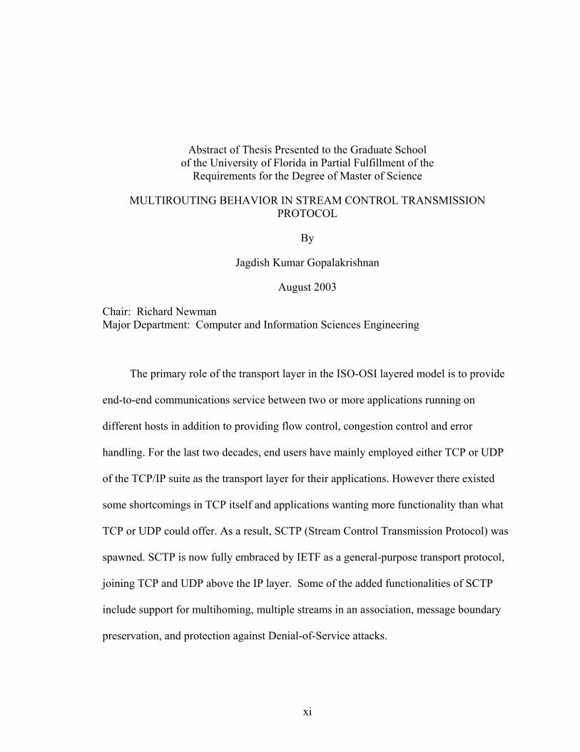
The primary role of the transport layer in the ISO-OSI layered model is to provide
end-to-end communications service between two or more applications running on
different hosts in addition to providing flow control, congestion control and error
handling. For the last two decades, end users have mainly employed either TCP or UDP
of the TCP/IP suite as the transport layer for their applications. However there existed
some shortcomings in TCP itself and applications wanting more functionality than what
TCP or UDP could offer. As a result, SCTP (Stream Control Transmission Protocol) was
spawned. SCTP is now fully embraced by IETF as a general-purpose transport protocol,
joining TCP and UDP above the IP layer. Some of the added functionalities of SCTP
include support for multihoming, multiple streams in an association, message boundary
preservation, and protection against Denial-of-Service attacks.
xi

By default, the SCTP protocol supports only one active path for data transmission
during the lifetime of an SCTP association. The other paths, if any, are used as standby
paths for the purpose of fault tolerance in case the main primary path goes down. In this
thesis, we make use of the best path in terms of the transmission time along that path and
hence over-riding the idea of a single permanent primary path throughout the lifetime of
an association. By measuring the RTTs (Round Trip Times) of all paths that exist in an
association, the primary path can be changed to the path of least RTT. After studying the
basic multirouting behavior in SCTP, we propose many design changes to the protocol to
increase the data throughput. We implement many combinations of the solutions
proposed, in addition to basic multirouting, to increase the rate of data transmission.
Simulation tests are run in NS-2 to test all the different solutions implemented. In
the end, we prove that by having the multirouting, SCTP performs better in terms of
higher rate of data transmission.
xii

CHAPTER 1 INTRODUCTION TO MULTIROUTING
In this chapter, we give brief introductions to TCP, and SCTP, and their
drawbacks and advantages. This chapter also provides a general overview of the
multirouting feature in SCTP, which is the crux of the thesis. In the end, a roadmap to
further chapters ahead is provided.
1.1 Transmission Control Protocol (TCP)
The Transport layer is one of the four layers in the TCP/IP model, which
superseded the earlier ISO-OSI model. It is sandwiched between the application layer and
the Internet layer. The most important role of the transport layer is to provide end-to-end
communication service between two or more applications on different hosts in a network.
TCP, which is a connection-oriented transport layer protocol and UDP, the
connectionless transport layer protocol, have been most dominantly used in today’s
networks. Many new transport layer protocols had been proposed to replace TCP/UDP
and overcome their shortcomings. But they have simply failed to make even a minimal
impact in the domain of transport layer protocols.
Some of the shortcomings of TCP have been summarized as follows:
• Many applications face the problem of Head-Of-Line blocking when TCP forces a strict ordering of segments to be passed to the application.
• It is sometimes necessary to logically distinguish between the different bytes or streams of data sent, whereas in the case of TCP, it is just a raw sequence of bytes.
• TCP does not support multihoming. A TCP connection is strictly defined by the communication by means of sockets between a pair of IP address and a port on one end and another pair of IP address and port on the other. TCP will not be able to
1
2
use the multiple addresses that exist in a multihomed host as a part of the same TCP connection.
• TCP is vulnerable to Denial-Of-Service attacks, where the TCP server allocates space for the TCB (Transmission Control Block) in it’s kernel before the client reaffirms its genuine intention of communication with the server, by acknowledging the SYN-ACK segment sent by the server.
• Multiple Streams of data cannot be sent in a single TCP connection.
1.2 Stream Control Transmission Protocol (SCTP)
SCTP was introduced in the October of 2000, primarily as a transport protocol in
the PSTN (Public Switched Telephone Network) backbones for carrying the signaling
information. SCTP also eliminated the Head-Of-Line blocking and preserved the
message boundary by having different chunks for control and data. Most importantly it
supported the concept of multihoming, where multiple IP addresses of a multihomed host
can be used as part of a single SCTP association. SCTP also provides a solution for
Denial-of-Service attacks by postponing the allocation of the memory in the stack for
TCB until the client firmly commits to continuing the relationship with the server.
In brief, other than fixing the defects of TCP, SCTP is very similar to TCP in
other respects. SCTP follows the same congestion control features as TCP namely slow-
start, congestion avoidance, fast retransmit and fast recovery. SCTP provides for the
Selective Acknowledgments (SACKs) like TCP to allow for partial acknowledgments of
segments received in non-sequential order. As a result of SCTP’s close resemblance to
TCP, the IETF (Internet Engineering Task Force) declared SCTP as a general transport
layer protocol other than its use in signaling networks. The details are further elaborated
in the next chapter.

3
1.3 Multirouting in SCTP
As stated in the RFC 2960 for SCTP [1], there is only one primary path used for
data transfer in the case of a multihomed SCTP association. The other paths are used for
fault tolerant purposes and become the primary path only when the current primary path
goes down. Each of the paths that exist can have a different transmission characteristic
such as bandwidth, delay, jitter etc., and hence we propose this multiroute feature to be
added to the SCTP protocol. We have considered the delay characteristic of each path in
evaluating a path and then decide whether a switch to the path of lower delay is to be
made.
The number of paths is dependent on the number of IP addresses exchanged
during the set up of an association. The delay information of each path is collected
periodically by means of the SCTP chunks sent out to check if a particular standby path is
alive or not. In implementing this feature, we do not straightaway achieve the goal of
higher data transmission. We encounter problems of retransmission, limited growth of the
congestion window of the new path and the generation of duplicate acknowledgements
with this naïve approach of multiroute, which prevent us from achieving higher rate of
transmission.
Each of the problems is fixed individually as we finally arrive at the combination
of various solutions to finally accomplish our objective of an increased rate of data
transmission, as compared to the unmodified SCTP.
1.4 Roadmap Ahead
We start the formal discussion in the second chapter, where the basics of TCP, the
congestion control algorithms of TCP and the different flavors of TCP are explained.
4
SCTP is introduced later in the chapter along with its different chunk formats and it
concludes with the connection establishment and termination.
In the third chapter, we elaborate on the design of the naïve multiroute feature.
The various design issues and problems encountered in the basic implementation of
multiroute are explained. We also arrive at a matrix representation of the combinations of
the different categories of solutions.
In the fourth and fifth chapters, the implementation details of the three solutions
that we proposed to incorporate efficient multirouting in the SCTP protocol are dealt
with. We progressively analyze the behavior of SCTP for each of the implementations,
by using a particular network scenario in Ns-2 (Network Simulator). Results are then
graphically compared with the results obtained with the results of unmodified SCTP in
terms of the number of segments transmitted in unit time (20 seconds).
In the sixth chapter, the simulation results are restated and evaluated against the
metric, which is the number of data segments transmitted in unit time, i.e., bytes per
second. We find that by embedding the efficient multirouting in the SCTP stack as we
have done, we are able to ultimately achieve a higher rate of data transmission.
We conclude in the seventh chapter by summarizing all the activities carried out
and the results obtained in this thesis. In an orientation towards future research, a few
interesting ideas and projects that can be done in the area of SCTP are listed.
CHAPTER 2 INTRODUCTION TO TCP AND SCTP
This chapter explains the basics of TCP, its different flavors and goes on to discuss the
congestion control algorithms in TCP. It also gives an introduction to SCTP, the different
chunk formats in SCTP, the establishment of an SCTP association and concludes with the
differences between TCP and SCTP.
2.1 Transmission Control Protocol (TCP)
2.1.1 OSI and TCP/IP models
The ISO (International Standards Organization) is responsible for the genesis of
the seven-layered layered model ISO-OSI (Open Systems Interconnect) to define the
functionalities of the different layers of the network operating system. Each of the seven
layers namely the Application layer, Presentation layer, Session layer, Transport Layer,
Network layer, Data link layer and the Physical layer, was defined with clearly defined
interfaces and input/output for interaction between the different layers.
In what was started as a defense research project for the Department of Defense
(DOD), the TCP/IP model was commercially introduced shortly after. It superseded the
OSI model and is most widely used today. TCP/IP model does not exactly match with the
OSI model. All the functionalities of the seven layers of the OSI model were reduced to
four layers in the TCP/IP model namely Application layer, Transport layer, Internet
Layer and the Network Access layer.
5
6
2.1.2 Transport Layer
The Transport Layer’s primary role includes providing end-to-end communications
between two or more applications running on different hosts. The other functionalities of
the transport layer is summarized as follows [1]:
• Manage the flow control of data between peers across the network.
• Provide error checking to guarantee error-free delivery of data.
• Guarantees a reliable data transfer by providing acknowledgements (ACKs) for data chunks received.
• Retransmission of lost segments.
• Follows efficient congestion control algorithms to stabilize the flow of data in case of congestion in the network.
There are two transport layer protocols in the TCP/IP model. One is the reliable
connection oriented Transmission Control Protocol (TCP) and the other is the
connectionless User Datagram Protocol (UDP). UDP does not perform any end-to-end
reliability checks. Our focus in the thesis as a whole is on the transport layer.
2.1.3 Basics of TCP
As mentioned earlier, TCP is a reliable connection oriented protocol and based on point-
to-point communication between two network hosts. Before a peer can start sending data
through a TCP connection, a TCP session has to be established between the two hosts.
The host initiating the TCP association (client) and the receiving host (server) are said to
perform the active open and the passive open respectively. The server waits on a well-
known port to provide a particular service, which enables clients to connect to it. Some
well known TCP ports used by standard TCP-based programs are 20 (FTP data channel),
21 (FTP control channel), 23 (Telnet), 53 (Domain Name System), 80 (Webserver-
HTTP) etc.

7
Richard Stevens defines a connection to be the communication link between two
processes, i.e., a client and a server [2]. An association is used to define a 5-tuple that
completely specifies the two processes that make up a connection:
{ protocol, local-addr, local-process, foreign-addr, foreign-process }
The protocol we use here is TCP. The local-addr is the IP address of the network
interface used by the client for data transmission. Local-process is a local port used to
identify the application that is to receive the data received on this connection. Foreign-
addr is the IP address of the network interface of the peer or the server, which the client
communicates with. Foreign-process is nothing but the well-known ports.
2.1.4 TCP Connection Establishment
Establishment of a TCP connection involves the creation of sockets at both ends
of the connection. A socket is defined as the one end-point of a two-way communication
link between two programs running on the network. Socket APIs (Application Program
Interfaces) provide an application interface to the communication protocols. Socket APIs
such as socket, accept, bind, connect, listen, send, recv etc. are used for the setting up of
the connection and the transmission of data along a connection.
The TCP session is established by means of a 3-way handshake where the client
initiates an active open and sends a TCP-SYN segment to the server. The TCP-SYN
segment contains the client’s initial sequence number. The server, on passive open,
accepts the TCP-SYN segment and acknowledges it by sending a SYN-ACK segment.
The SYN-ACK segment also contains the initial sequence number of the server. The
client on receiving the SYN-ACK acknowledges it by sending an ACK to the server. This
is the 3-way handshake protocol used for establishment of a TCP connection and is
depicted in the diagram below.

8
Figure 2-1: The 3-way handshake used for TCP connection establishment
2.1.5 TCP Congestion Control
A retransmission timer is started at the sender side when a segment is transmitted.
This expires if the segment is not ACKed within a certain time duration depending on the
RTT of the path. The expiry of the retransmission timer indicates a lost segment and the
segment is immediately retransmitted before any new data segments are transmitted.
In the next section, we look at four algorithms, namely, slow start, congestion
avoidance, fast retransmit and fast recovery [2,3]. Before moving on to the TCP
congestion control algorithms, we need to look at a few variables maintained in the TCP
stack for following the rules of congestion.
• Cwnd: This is the congestion window variable maintained in bytes by either ends of the connection. This value is used to control the flow of data from the sender side. The sender, at any time can transmit up to the minimum of the congestion window and the advertised receiver window (rwnd).
• Rwnd: This is the value in bytes advertised by the receiver as to the no of bytes of space available in the receiver buffer for the sender to fill up. In other words, rwnd
9
is nothing but the flow control imposed by the receiver. As mentioned before, a sender can only transmit up to the minimum of the value of cwnd and rwnd.
• Ssthresh: This is the slow start threshold. Slow start is discussed in the next section. When the value of cwnd is less than or equal to ssthresh, then slow start algorithm is followed or else congestion avoidance algorithm is followed.
2.1.5.1 Slow start and Congestion Avoidance
• Initially the values of cwnd and ssthresh are set to 1 or 2 times SMSS (Sender Maximum Segment Size) bytes and 65,535 bytes respectively. This is because when the connection is started, TCP does not know the conditions of the network and hence it starts to experiment slowly by setting cwnd to 1 or 2 SMSS bytes.
• During the period of slow start, i.e., as long as cwnd is less than or equal to ssthresh, for each ACK received that acknowledges new data, TCP increases the value of cwnd by at most SMSS bytes
• When the value of cwnd is greater than ssthresh, the congestion avoidance phase kicks in. In congestion avoidance, the value of cwnd is incremented by 1 full sized segment per RTT (Round Trip time). Congestion avoidance is continued till the congestion is detected. A commonly used formula used to affect the value of cwnd during congestion avoidance is as follows:
cwnd += SMSS * SMSS / cwnd
• When congestion occurs (indicated by a timeout or the receipt of duplicate ACKs, values of cwnd and ssthresh are affected as described in the next section.
2.1.5.2 Fast retransmit and Fast recovery
Fast Retransmit and Fast Recovery algorithms are usually implemented together as
indicated by the following steps:
1. A TCP receiver has to immediately notify the other end if there are any gaps in the segment numbers that it receives. So it generates a duplicate ACK whenever an out-of-order segment is received. If the sender receives three such duplicate ACKS, it is definitely a strong indication that a segment is lost.
2. When the sender receives three duplicate ACKs, then it retransmits the missing segment without waiting for the retransmission timer to expire. This is the fast retransmit algorithm. Now the value of ssthresh is set to the maximum of the values of (FlightSize / 2) and 2 * SMSS.
ssthresh = max (FlightSize/2, 2 * SMSS).

10
FlightSize is nothing but the number of outstanding bytes maintained at the sender end, which have not yet been acknowledged by the receiver.
The new value of the cwnd is set to ssthresh plus 3 times the segment size.
3. Additionally if the congestion is indicated by a timeout, then slow start algorithm is again followed.
4. Each time another duplicate ACK is received, increment cwnd by SMSS and transmit the packet if allowed by the new value of cwnd.
5. When the next ACK acknowledging the new data arrives, set the value of cwnd to ssthresh (which is the same value set in step 1). This ACK should also acknowledge all the segments sent between the lost packet and the receipt of the third duplicate ACK.
2.1.6 Different Flavors of TCP
Since TCP was originally introduced, it has undergone a lot of modifications to
yield better performance. In this section we briefly look at a few flavors of TCP in the
recent years.
2.1.6.1 Tahoe TCP
The base version of TCP did very little to combat congestion and used the go-
back-N model to go back N segments and retransmit all the data lost following the
expiration of the retransmit timer. The congestion algorithms such as the slow start,
congestion avoidance and fast retransmit algorithms discussed in the previous section
were added to the base version of TCP resulting in Tahoe TCP. It also included the
modification to the round-trip time estimator to set the retransmission timeout values.
This led to better bandwidth utilization and throughput than the base version.
2.1.6.2 Reno TCP
Reno TCP contained all the modifications incorporated into Tahoe TCP, but also
included the fast recovery algorithm discussed in the previous section. At the receipt of
three duplicate ACKs, the Tahoe sender used to go into slow-start after retransmitting the
11
missing segment. But Reno TCP decreases the congestion window by one half and uses
incoming ACKs to increment the congestion window. Since the receiver can only
generate the duplicate ACK when another segment is received, that segment has left the
network and is in the receiver’s buffer. This means that there is still data flow going on
between the sender and the receiver, and this should not abruptly be reduced by following
the slow start. Hence the value of cwnd is set to a higher value as described in the slow
start section.
Reno TCP shows a better and optimized performance than Tahoe TCP when a
single packet is dropped from a window of data. But the performance can be affected
when multiple packets are dropped from a window of data.
2.1.6.3 Vegas TCP
Vegas TCP showed a further 40% – 70% improvement in the throughput as
compared to the Reno implementation of TCP [4]. A new retransmission policy is used in
Vegas. In Reno, the arrival of three duplicate ACKs trigger the process of retransmission,
but Vegas uses a time stamp for each packet sent to calculate the RTT on each ACK
received. If the difference between the timestamp for that packet and the current time is
greater than the timeout value, then Vegas TCP retransmits the packet without waiting for
the third duplicate ACK from the receiver. If there are any losses of ACKs since the
retransmission, then the segments are retransmitted without the wait for duplicate ACKs.
A comparison of the actual throughput and the expected throughput to the
threshold values is made and then the window size is decreased or increased linearly.
2.1.6.4 TCP-SACK
SACK stands for Selective ACKs [5]. Initially the base implementation of TCP
used the cumulative acknowledgement scheme, in which the non-contiguous segments

12
received after the highest numbered segment in sequential order, were not acknowledged.
This made the sender to either wait for one RTT to detect each lost packet or retransmit
the segments even though they have reached the receiver albeit in non-sequential order.
Thus the TCP-SACK option was introduced which could inform the sender about the
highest numbered segment received in order and the non-contiguous segments received.
Since this is an extension to the base TCP, some TCP versions may support it whereas
many may not. Hence it becomes essential at the time of the connection establishment to
decide whether both ends would follow the SACK option or not.
To indicate the non-contiguous segments received, the 40 bytes of TCP options in
the TCP header is made use of. A start block and an end block represent each block of
contiguous data in the set of non-contiguous data. The start block indicates the starting
sequence number and the end block represents the ending sequence number.
Sally Floyd has performed simulation-based comparisons of Tahoe, Reno and
SACK TCP [6].
2.1.7 TCP Connection Termination
• Since a TCP connection is full duplex, it needs to be shut down independently from both ends.
• To close a connection, a FIN segment is sent across to the other end. The receiver of FIN segment sends an ACK of the FIN segment. The end that issues the close first performs the active close and the other end performs the passive close.
• After one end does the active close, the other end does the passive close.
• When the FIN segment is received, there will not be any more data flow from the sender of the FIN segment.
• After an end sends across the FIN segment, it can still receive the data from the other end. This is known as the half close connection when the peer that has sent the FIN segment and received the ACK for the FIN, is waiting for the FIN segment from the other peer.

13
The connection termination is shown in figure 2-2.
Figure 2-2: TCP Connection termination.
2.8 Shortcomings of TCP and the Origin of SCTP
For the last two decades, the TCP/IP suite (which is slightly different from the
OSI suite) has dominated the networking world. Either TCP (Transmission Control
Protocol) or the UDP (User Datagram Protocol) has been used widely used in
applications worldwide as a transport layer protocol. Some applications using TCP,
however, needed additional features than what TCP currently offered. There were a few
vulnerable factors about using TCP, which we will describe shortly.
Ivan quotes the following deficiencies in TCP [7]:
• Many applications such as the streaming video do not require the strict ordering of segments before passing them on to the application. This produces Head-Of-Line (HOL) blocking. In this case TCP would produce the unnecessary delay in strict ordering. Therefore a transport layer protocol, apart from providing the connection oriented features also needed to have an option of unreliable and non-strict or partial order delivery of segments to the application.

14
• TCP treats data transmission as an unstructured sequence of bytes. Streams cannot be logically demarcated and it is up to the application to insert their marks inside the streams explicitly.
• TCP does not support the concept of multihoming. Multihoming is the ability of a host to support multiple IP addresses. It is not possible to associate more than one IP address of a host to one end as a part of the same TCP connection. Thus a host with multiple interface cards will not be able to use all its IP addresses as a part of the same TCP connection. The reason for using the multiple IP addresses as a part of an association could be for the reasons of load sharing or fault tolerance. We will discuss these issues in the coming sections.
• TCP is vulnerable to Denial-Of-Service (DOS) attacks or SYN attacks. This happens during the three-way handshake of the TCP connection initialization. The entity, which does the passive open of the TCP connection, always allocates resources for an impending TCP connection after it receives a SYN segment and responds with a SYN-ACK. The application that does the active open may not respond with the ACK and may not complete the three-way handshake. This activity, when repeated, may exhaust the kernel resources to start a fresh TCP connection and ultimately it becomes impossible to spawn TCP connections.
• TCP does not allow applications to have control over the TCP timers like the initialization timers, retransmission timers etc.
One of the main applications, which found these above features of TCP lacking,
was the transport of PSTN (Public Switched Telephone Network) signaling across an IP
network. Thus, to overcome all these deficiencies of TCP, MDTP (Multi-Network
Datagram Transmission Protocol) was introduced by Randall Stewart and Qiaobing Xie.
Later on, they modified this to introduce SCTP. SCTP was initially called Signaling
Common Transport Protocol. But later, it was realized that SCTP could be used as an
alternate for TCP for normal networking applications other than signaling transport. The
reasons being that it behaved in a similar manner as TCP in addition to overcoming the
above mentioned limitations. So it was renamed to Stream Control Transmission
Protocol.

15
SCTP is a very recent transport protocol dating back to October 2000 when Randall
Stewart et al introduced the RFC 2960 [8], which formally describes SCTP.
2.9 Features of SCTP
We describe below, the features of SCTP in contrast to deficiencies of TCP and the
general features offered:
• Head-Of-Line (HOL) blocking is eliminated by SCTP as it also provides an option for both sequenced delivery of segments and unordered delivery of segments to the application. It supports both TCP and UDP modes of delivery.
• Having separation between logically structured sequences of bytes called chunks, preserves message boundary. Thus control information and the actual data can be grouped into separate chunks.
• SCTP provides support for multihoming. During the phase of establishment of an SCTP association, either side can include one or more IP addresses as a part of the association. A feature to include the IP addresses dynamically in the middle of an association is also being provided currently [9]. However as we will discuss later, only one path between a pair of IP addresses is allowed to be the primary path for communication between two end points. Using the feature of multihoming, the probability of the data chunks that have been transmitted, reaching their destinations will be increased [10].
• SCTP supports multiple streams of data in a single association. To create the independence in data transmission and data delivery, two sets of sequence numbers are used: a unique Transmission Sequence Number (TSN) for each data chunk and a unique Stream Sequence Number (SSN) to identify a data chunk within a particular stream [10].
• SCTP prevents the Denial-Of-Service attacks by using a 4-way handshake it uses while starting a new association. We will describe the 4-way handshake in the later sections of this chapter. Basically SCTP does not allocate any resources when it receives an INIT (the equivalent of a TCP SYN) from a client. Instead it forms a cookie that embeds all the information required for forming a connection (information required to form a Transmission Control Block) and sends it across to the client. Only when the client echoes back the cookie to the server, will the actual allocation of resources take place at the server end.
• SCTP follows TCP- friendly congestion control algorithms. This includes the slow-start, congestion avoidance and retransmission algorithms of TCP. SCTP also derives the Selective Acknowledgement (SACK) derived from TCP. It provides a GAP ACK block that includes information about non-contiguous segments that are missing at the receiver end.
16
• SCTP has a Heartbeat chunk which are sent periodically along the different paths of an association. By this mechanism it decides whether a particular endpoint or interface of the other end has failed. This feature is currently used in SCTP as a fault tolerance mechanism.
• User data is fragmented to fit the Maximum Transmission Unit (MTU) along a particular route.
• A mandatory Verification tag field and a 32 bit check sum (Addler checksum) is added to the SCTP header for validation after an endpoint receives a packet.
• Any application running over TCP can be ported to run over SCTP.
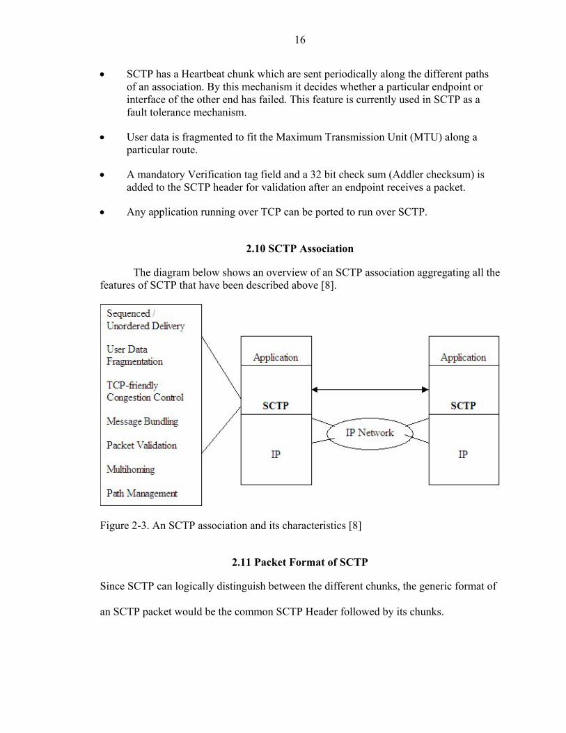
2.10 SCTP Association
The diagram below shows an overview of an SCTP association aggregating all the features of SCTP that have been described above [8].
Figure 2-3. An SCTP association and its characteristics [8]
2.11 Packet Format of SCTP
Since SCTP can logically distinguish between the different chunks, the generic format of
an SCTP packet would be the common SCTP Header followed by its chunks.

17
Figure 2-4: SCTP Packet format
2.12 SCTP Chunk Description
Each SCTP chunk is specific to its functionality. The Chunk has information
about the Chunk Type, different flags for that chunk, length of the chunk and the value of
the chunk (data). The general format of an SCTP chunk is shown below:
Figure 2-5: SCTP Chunk format [8]
• Chunk Type: This field is an 8-bit unsigned integer. There can be various chunk types like INIT, DATA, INIT-ACK etc. A short description of some of the relevant chunks is described in the next section.
• Chunk Flags: This is of 8 bits. This contains information pertaining to a particular chunk.
• Chunk Length: This is a 16-bit unsigned integer and contains the length of the chunk in bytes. This field does not include the length of the padding.
• Chunk Value: This is a variable length field containing the actual data to be transmitted. The type of data it carries is dependent on the type of the chunk.

18
2.13 SCTP Common Header
SCTP Header is similar to the TCP Header with information such as the source
port number, destination port number, and check sum. It also contains the verification tag
for validation purposes. Fields such as Acknowledgement number, sequence number etc.
found in the TCP header are not found in the SCTP Header. Since there is message
preservation in SCTP and the existence of chunks, the individual chunks carry this
information. Figure 2-6 shows the SCTP Header.
Figure 2-6: SCTP Common Header format
• Source Port Number: This is a 16 bit unsigned integer. It contains the port number of the SCTP sender.
• Destination Port Number: This is a 16 bit unsigned integer. It contains the port number of the SCTP destination.
• Verification Tag: This is a 32 bit unsigned integer. This is used to check if the packet is coming from a valid and right host. It contains the value that was agreed upon while sending the INIT and INIT-ACK chunks during the initialization of the SCTP association.
• Checksum: This is a 32 bit unsigned integer containing the checksum of the SCTP Packet.
19
2.14 Various SCTP Chunk Descriptions
Depending on the value of the chunk type, we have various chunks that are
described in this section.
2.14.1 INIT Chunk
This chunk is analogous to the TCP SYN segment sent during the initialization of
the segment. This contains an initiate tag, used as a verification tag in all other segments
sent by the receiver of the INIT. The use of the verification tag has already been
discussed earlier. The number of inbound and outbound streams in the association is also
negotiated during the sending of this chunk. The INIT chunk also contains the receiver
window size that is advertised along with one or more IP addresses that would be used
during the association to support multihoming. The Initial Sequence Number (ISN) is
also a part of the INIT chunk.
2.14.2 INIT ACK Chunk
This chunk is sent in response to an INIT chunk. The format of this chunk is
similar to the INIT chunk except that it also contains the State Cookie, which is generated
by the sender of the INIT ACK chunk. As described earlier, this is a method to prevent
the Denial-Of-Service attacks.
2.14.3 DATA Chunk
This carries the user data along with the information such as the TSN
(Transmission Sequence Number), Stream Sequence number (since multiple streams can
be transmitted as a part of a single association) etc. The fields just described are
analogous to the Sequence number in TCP, except that they have been moved to the
chunks from the header portion.

20
2.14.4 SACK Chunk
This is the Selective Acknowledgement Chunk. As the name indicates, this chunk
is used to acknowledge data where the Transmission Sequence Number (TSN) of the data
received may or may not be in a sequence. To indicate non sequential data received, this
chunk has a GAP ACK block, which has a GAP ACK start number and a GAP ACK end
number indicating the TSNs of the chunks received. This chunk also has a duplicate TSN
block to let the sender know of any duplicate chunks received. It also carries the
Cumulative TSN ACK, which contains the TSN of the last DATA chunk received in
sequence before a gap.
2.14.5 HEARTBEAT Chunk
HEARTBEAT chunks are usually sent to detect the reachability of a destination.
This normally includes the information about the sender’s current time when the
HEARTBEAT is sent.
2.14.6 HEARTBEAT ACK Chunk
HEARTBEAT ACK chunks are sent in response to HEARTBEAT chunks. It is
always sent to the source IP address of the datagram containing the HEARTBEAT chunk.
2.14.7 ABORT Chunk
ABORT chunks are sent to shut down an association abruptly. It also contains the
error code as to why the association was terminated. DATA chunks must not be bundled
with the ABORT chunk.
2.14.8 SHUTDOWN Chunk
SHUTDOWN is sent to facilitate a graceful shutdown of an SCTP association. It also
contains the Cumulative TSN Ack, which is the TSN of the last chunk received in
sequence before any gaps.

21
2.14.9 SHUTDOWN ACK Chunk
SHUTDOWN ACK is sent in response to a SHUTDOWN chunk.
2.14.10 SHUTDOWN COMPLETE Chunk
SHUTDOWN COMPLETE is used to acknowledge the receipt of the
SHUTDOWN ACK chunk. This is sent at the end of the shutdown process.
2.14.11 ERROR Chunk
ERROR chunk is sent to indicate to its peer end point of an error condition. There
can be various error conditions such as Unresolvable Address, Unrecognized parameters,
Out of Resource etc.
2.14.12 COOKIE ECHO Chunk
This chunk is used in the initialization of an association. The peer end wanting to
initiate an association sends this chunk. This completes the initialization process from the
client side. This chunk must be sent before any DATA chunks can be transmitted.
2.14.13 COOKIE ACK Chunk
COOKIE ACK chunk is sent in response to a COOKIE ECHO chunk. Again,
before any DATA chunks can be transmitted, this chunk should be transmitted.
2.15 SCTP Association Establishment
SCTP has a 4-way handshake unlike TCP’s 3-way handshake in establishing an
association. The following are the steps involved in the 4-way handshake:
• One of the ends sends an INIT chunk with all the necessary information embedded in it. The sender of INIT now starts a timer, T1-init timer and enters the COOKIE-WAIT state.
• The receiver of the INIT chunk responds by sending an INIT ACK chunk. The verification tag in the INIT and INIT ACK chunks is used for validation purposes during future transmissions of data. The receiver now generates a cookie and

22
embeds in it, all the information needed to establish a TCB (Transmission Control Block) and sends it along with the INIT ACK. No resources are allocated at the receiver end for the TCB.
• When the sender of INIT receives the cookie from the peer end, it stops the T1-init timer and sends the cookie back in a COOKIE ECHO chunk. After this it starts the T1-cookie timer and enters the COOKIE-ECHOED state. The data transmission can actually start with this chunk.
• After receiving the COOKIE ECHO chunk, the peer establishes the TCB and changes to the ESTABLISHED state. It now sends a COOKIE ACK, which could also be bundled along with other data chunks.
• When the other end receives the COOKIE ACK chunk, it now moves to the ESTABLISHED state and stops the T1-cookie timer.
The diagram below shows the SCTP association establishment. The steps described
above can also be seen in the SCTP State diagram in the next section.
Figure 2-7: SCTP Association establishment.

23
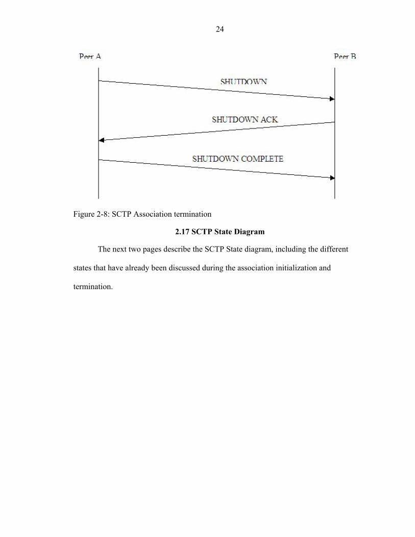
2.16 SCTP Association Termination
SCTP uses a 3-way handshake when the association has to be terminated unlike
TCP’s four exchanges for complete termination of the connection. The steps for a normal
and a graceful shutdown are described as follows:
• The application issues a SHUTDOWN primitive to the SCTP asking it to shut down the association. Since there is no concept of half closed states like in TCP, all the data has to be flushed out before sending the SHUTDOWN chunk. It now reaches the SHUTDOWN-PENDING state before the data is sent. After all the pending data is sent, a SHUTDOWN chunk is sent and moves to the SHUTDOWN-SENT state. It also starts the T2-shutdown timer.
• When the other end receives the SHUTDOWN chunk, it goes to SHUTDOWN-RECEIVED state. Now it is this end’s turn to send all the outstanding data to the other end. Also the SHUTDOWN receiver must not receive any fresh DATA chunks from the other end during this time. The SHUTDOWN sender now restarts the T2-shutdown timer each time it receives fresh DATA chunks and responds with a SACK. But the SHUTDOWN sender must not send data at this point of time. The SHUTDOWN receiver now sends a SHUTDOWN ACK chunk and moves to SHUTDOWN-ACK-SENT state.
• When the SHUTDOWN sender receives the SHUTDOWN ACK, it stops the T2-shutdown timer and sends a SHUTDOWN COMPLETE chunk to its peer and thus erases all traces of this association. Thus the association at this point of time is completely broken down.
The diagram 2-6 shows the steps in the SCTP termination. These states are also shown in
the SCTP state diagram later in the chapter.
24
Figure 2-8: SCTP Association termination
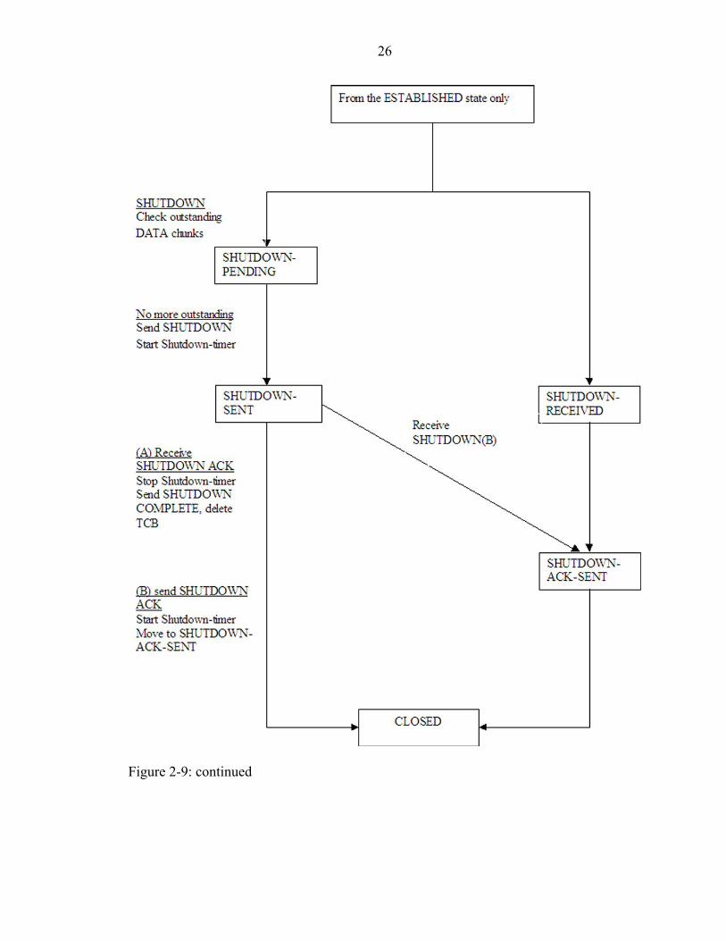
2.17 SCTP State Diagram
The next two pages describe the SCTP State diagram, including the different
states that have already been discussed during the association initialization and
termination.

25
Figure 2-9: SCTP State diagram
26
Figure 2-9: continued

27
2.18 SCTP Congestion Control
SCTP congestion control algorithms are very similar to the TCP congestion
control. It follows the slow start algorithm, congestion avoidance, fast retransmission and
recovery just like TCP. The one main difference between the TCP and SCTP congestion
control is that since SCTP supports multihoming, it is necessary to store and maintain the
congestion control parameters for all paths of a multihomed association. SCTP provides
for SACKs and GAP ACKs to indicate selective acknowledgement and gaps in the
received segments.
SCTP maintains three congestion control parameters:
• Congestion Control window (cwnd): This is maintained in bytes. This indicates a limit of how many bytes the sender can currently send to the peer end, provided the flight size and the receiver window permit it. Its function is similar to ssthresh in TCP.
• Slow Start threshold (ssthresh): This is stored in bytes and is used to distinguish between slow start and congestion avoidance. Its function is similar to ssthresh in TCP.
• Receiver Window size (rwnd): This is the limit set by the receiver as to how many bytes it can receive contingent on the buffer size and how much the application has emptied the receiver buffer.
It is again emphasized that there are separate variables stored for each of the
destination addresses. But only one rwnd variable is kept. Apart from these variables,
another variable partial_bytes_acked records the number of bytes that have been partially
ACKed by GAP ACKs and otherwise.
Slow start and congestion avoidance is similar to those of TCP except that
partial_bytes_acked also comes into the picture as described in the steps below.

28
2.18.1 Slow Start
Slow start algorithm is used to probe a network initially before injecting data into it
because one is not aware of the conditions of the network initially.
• The initial cwnd is set to 2 * MTU (Maximum Transmission Unit) bytes at the start.
• After a retransmission, the cwnd is set to 1 * MTU.
• The initial value of ssthresh is set to a high value like 65536.
• When the cwnd is less than or equal to ssthresh, then slow start algorithm is to be used. If an incoming SACK advances the Cumulative TSN ACK point (which is nothing but the highest TSN received in sequence so far), then cwnd must be increased by a minimum of either the total size of the DATA chunks acknowledged OR the destination path’s MTU.
• When an endpoint does not transport data on a given address, the cwnd of that path must be set to the maximum of (cwnd /2) OR 2 * MTU per RTO (Retransmission Time Out).
2.18.2 Congestion Avoidance
Congestion Avoidance is to be used when the value of the ssthresh is less than
cwnd.
• Initially partially_bytes_acked is set to zero.
• When cwnd is greater than ssthresh, each SACK that arrives increases partially_bytes_acked by the number of bytes acknowledged.
• When the sender has cwnd or more bytes of data outstanding and partial_bytes_acked is greater than or equal to cwnd, then increase cwnd by MTU bytes and reset partial_bytes_acked to (partial_bytes_acked – cwnd).
• Obviously when all the data has been acknowledged, partial_bytes_acked is reset to zero.
• Whenever data segments are indicated as missing by way of the SACKs or GAP ACKs, i.e., whenever the number of ‘missing segment’ reports reaches four, then it follows fast retransmission. Here the value of ssthresh is reduced to a maximum of (cwnd / 2) and 2 * MTU. The value of cwnd is now set equal to ssthresh, However if the retransmission timer waiting on the ACKs expires, SCTP performs slow start

29
by setting cwnd to 1 * MTU and ssthresh to a maximum of (cwnd / 2) and 2 * MTU.
2.19 SCTP Fault Tolerance
Like TCP, SCTP makes use of HEARTBEAT chunks to find out if a particular
destination is still alive or not. This is analogous to the keep-alive timer in TCP. The
following steps describe the operation of the heartbeat mechanism in SCTP:
• During the setting up of an association, the periodic interval at which HEARTBEAT chunks are sent to a destination is provided.
• After the heartbeat timer expires, the host sends HEARTBEAT chunks with the timing information in it.
• If the HEARTBEAT chunk is not acknowledged with a HEARTBEAT ACK within the RTO, then an error counter for that destination is incremented.
• When the error counter of a destination path reaches an upper bound, Path.Max.Retrans, then that path is declared inactive.
• But when the HEARTBEAT ACK is received from the destination, then the error counter is cleared.
• The receiver of the HEARTBEAT chunk copies the information from it onto a HEARTBEAT ACK chunk.
• The application can set the interval HB.interval, i.e., the interval at which HEARTBEAT chunks are to be sent out to a destination.
• Since the HEARTBEAT chunk contains the timing information as to when that particular chunk was sent, the RTT (Round Trip Time) of that path can be calculated and updated.
The SCTP HEARTBEAT chunks are similar to the TCP Keep-alive timer. The
option to enable the TCP keep-alive timer is provided by the setsocket() API of the
socket API. TCP sends a keep-alive packet periodically to check if the particular endpoint
is alive or not.
30
2.20 Security Issues in SCTP
SCTP mainly uses the verification tag and the cookie as security mechanisms in
addition to using the IpSec features of the network layer [11, 12]. SCTP as a protocol
does not define any new security protocols or procedures [10].
2.21 Key Points to Remember
In this chapter, we have discussed the basics of TCP, it’s different flavors, the
congestion control algorithms in TCP. We also discussed SCTP, its different chunks and
establishment and termination of an SCTP association.. We also summarized the
differences between TCP and SCTP.
In a TCP connection, there exists only a single path of communication between
two endpoints because a TCP connection is strictly between an IP address and a port on
one end and an IP address and a port on the other end. It does not support the concept of
multihoming. Therefore the issue of multipath routing does not arise at all in TCP, as it
does not support multihoming.
But in SCTP, since it supports the concept of multihoming, there exists multiple
paths as a part of a single association. Thus we should be able to use the different paths
provided as a part of the association after evaluating each one of them. In this manner, we
are able to realize the true utilization of all the paths as opposed to using a single path
during the duration of an association.
The HEARTBEAT chunks that we described have a significant bearing on the
topic of this thesis. As we see in the next chapter, it is the HEARTBEAT chunks using
which we decide whether to switch over to a new path and make it the primary
communication path. We make use of the timing information and calculate the RTT, in

31
order to switch over to a path that has the least RTT. We will discuss more about this in
the next chapter.

CHAPTER 3 DESIGN OF NAÏVE MULTIROUTING (MROUTE)
This chapter discusses the motivation for introducing the multirouting feature in the
SCTP protocol. It also explains the problems we faced with a naïve multirouting feature,
which we called MROUTE. The categories of problems that we face in MROUTE and
the solutions that we propose are presented in the form of a matrix. The various design
issues and decisions that were made are also elaborated.
Table 3-1: Summary of the differences between TCP and SCTP. TCP SCTP Head-of-line blocking due to the strict ordering of segments produces unnecessary delay in certain applications.
Head-of-line blocking is eliminated as SCTP supports both the options of both strict and non-strict ordering of segments. It supports both a TCP mode and a UDP mode of transmission.
Data transmission is treated as an unstructured sequence of bytes with no differentiation between streams.
Separation exists between logically structured sequences of bytes known as chunks.
Multihoming support is not provided. Multihoming support is provided with the ability to dynamically add/remove IP addresses in the middle of an SCTP association.
Vulnerable to Denial-of-Service attacks. Due to the cookie mechanism during the initialization of the association, Denial-of-Service attacks can be avoided.
Application control over the TCP timers does not exist.
Application control over SCTP timers is possible
Keep-alive timers are used to detect if a destination is alive or not.
HEARTBEAT chunks are used to detect if a destination is alive or not.
No scope for multipath routing as the support for multihoming is not provided.
Multipath routing is possible making use of the property of multihoming.
If the path of communication goes down, there is no fault tolerance provided, as there are no standby paths.
Through the support for multihoming, fault tolerance is provided by means of the other paths functioning as standby paths.
32
33
In the previous chapter, we talked about TCP, SCTP and the differences between
them. The above table briefly summarizes the differences between TCP and SCTP.
3.1 Motivation for Multirouting
According to the SCTP RFC [8], there is only one active path where the primary
communication of data takes place during a SCTP association. If the association is
multihomed, the other paths exist just as standby paths. If the primary path goes down
due to some reason, a standby path is made the primary path.
The choosing of the primary path currently does not depend on any criterion. By
default the path connecting the source IP addresses of the datagram containing the INIT
and the INIT ACK chunks is chosen as the primary path for communication. The other IP
addresses, which exist as a part of a multihomed association, are specified in the INIT
and INIT ACK chunks. The other paths are never evaluated and come into play only for
the purpose of fault tolerance.
The network conditions such as failures and congestion change dynamically all
the time. Hence we argue that using just one primary path for communication does not
utilize the multihoming feature of SCTP completely. As a result, we propose that the
other paths should be evaluated and used, when they become better than the primary path
currently used for transmission. Now the question of how a particular path is chosen over
other paths comes into consideration.
3.2 Design of Naïve Multirouting or MROUTE
We mentioned that the HEARTBEAT chunks are sent out periodically to detect
whether a particular destination is alive or not. We also recall that HEARTBEAT chunks
contain timing information and this is used to update the RTT (Round Trip Time)
estimators.
34
Round Trip Time is one of the critical factors influencing the throughput of data
transfer. If there are two paths of different RTTs, then the path with the lower RTT will
ultimately yield a higher rate of data transmission than the path with the higher RTT. The
RTTs of the various paths are updated when the HEARTBEAT ACK chunks arrive along
them. The RTT of the primary path is known since there is a regular flow of DATA
chunks along it. Thus the information about the RTTs of all the paths is available at any
point of time.
Hence whenever RTT of a particular path is updated we compare the RTTs of all
the paths and then decide whether primary path needs to be changed based on the
comparison. Whenever the primary path is changed to another path, then the data transfer
takes place along the new path chosen till another path of lesser RTT is available.
We now look at the various functions in the SCTP source code that are used when
the multirouting feature is introduced.
3.2.1 RttUpdate()
RttUpdate is a function that updates the RTT of a path, which it takes in as a
parameter. The function prototype is as follows:
void SctpAgent::RttUpdate(double dTxTime, SctpDest_S *spDest)
• dTxTime is the time stamp information. • SpDest is the destination, whose RTT needs to be updated based on dTxTime and
the current time. 3.2.2 ProcessHeartbeatAck()
ProcessHeartbeatAck, as the name suggests, is the function that is called
whenever a HEARTBEAT ACK is received in response to a HEARTBEAT chunk. In
short, this function clears the error counter associated with a specific destination and
based on the time stamp received, updates the RTT of the path. Error counter keeps track

35
of the number of times that the HEARTBEAT ACK was not received, before it declares
the other end as dead. The prototype of the function is as follows:
void SctpAgent::ProcessHeartbeatAckChunk( SctpHeartbeatAckChunk_S
*spHeartbeatAckChunk)
• SpHeartbeatAckChunk is the structure containing the HEARTBEAT ACK chunk. 3.2.3 SendBufferDequeueUpto()
When DATA chunks are transmitted, they are stored in the SendBuffer till the
other end acknowledges them. Whenever a SACK is received, then this function is called
to dequeue the DATA chunks from the SendBuffer. Only those DATA chunks that have
been acknowledged will be dequeued from the SendBuffer. After they are dequeued, the
RTT information is updated and the timer is stopped if the destination timer was still
running.
Thus we can see that there are two instances where the RTT information needs to
be updated. Both the ProcessHeartbeatAck() and SendBufferDequeueUpto() functions
need to call RttUpdate() as shown in the following diagram.
Figure 3-1: The calling of function RttUpdate
36
After the RTT information is updated in the function RttUpdate, we compare the
RTTs of all the paths. The multiple IP addresses of the peer end may be set up during the
association set up or by dynamically adding the IP address in the middle of an association
[9]. We then change the primary path of communication to the new path if it is found to
be of lesser RTT. Otherwise we continue transmission along the old path.
We call this the naïve multiroute or MROUTE since we do not make any other
modifications to the code and expect it to prove beneficial in terms of the rate of data
transmission. Logically speaking, the change of path to that of a lesser RTT should
improve the performance with respect to the throughput or increased rate of data
transmission.
3.3 Problem Areas of MROUTE
We discuss the implementation details of MROUTE and other solutions in the next
chapter. Before going on to the next chapter, the problems that we faced with the naïve
multirouting feature are listed. The problems associated with MROUTE can be
categorized into 4 classes:
1. Initial Cwnd Problem: The initial value of the cwnd of the new path determines how many segments we transmit initially. Different solutions to start the cwnd of the new path with a higher value are discussed. One of the solutions that we discuss in this category is the hysteresis method, where history of collected data pairs of (cwnd, RTT) would help in choosing an appropriate path.
2. Retransmission problem: As we will see in the analysis of our results in the next chapter, retransmission of segments takes place due to segments on the new path reaching the destination before earlier transmitted segments. Retransmission consumes considerable time and network resources. Alternatives to prevent this behavior are discussed.
Here we discuss the solutions of ignoring GAP ACKs (IGNORE) and preventive retransmission in addition to the default, unmodified behavior of SCTP.
3. Cwnd growth: After we follow one of the solutions that we list for the Initial Cwnd problem, the growth of cwnd from that point on affects the rate of data

37
transmission. We look at the different alternatives that can be followed for the cwnd growth.
In this category, we address solutions like increasing the cwnd of the new path based on the old path.
4. Oscillation: Basically this problem arises due to the occurrence of too many path changes in a given time and may bring about instability in the system. The Hysteresis method handles this problem to some extent. The research on this topic is not carried out in this thesis and is reserved for future work.
3.4 Key Points to Remember
Solutions to the first three categories of problems are listed in table 3-1. We
address each of these solutions and discuss the pros and cons of each one of them in the
next chapter.
Table 3-2: A tabular representation of the solutions.
Initial Cwnd Retransmission Method Path
Change (Y / N)
Default(1)
Hysteresis Value
Old-path
Default Preventive Retransmission
Ignore GAP ACKs
UNMOD N × × MROUTE Y × × IGNORE Y × ×
INC Y × × CwndOLD Y × × Or × Cwnd Growth
Method
Path Change (Y / N)
Default Use SACKs to increase cwnd
UNMOD × MROUTE × IGNORE Y ×
INC Y × CwndOLD Y × Or ×
Default solutions in each of the categories shown above indicate the current,
unmodified default behavior of the SCTP protocol, which we call UNMOD. We have
named the different combinations of the solutions that we have tried out as UNMOD,

38
MROUTE, IGNORE and INC. As indicated in the table, the cross symbol (×) shows the
combination of solutions that we tried out for each of the methods that we mention.

CHAPTER 4 IMPLEMENTATION AND ISSUES OF MROUTE
We discussed the design of naïve multirouting or MROUTE in the previous
chapter. We also addressed the problem areas in this design and came up with a tabular
representation of the different alternatives along with a brief introduction to each of the
problems. Before we elaborate on the details of the solutions, we give an introduction to
Network Simulator –2 (Ns-2) using which we carry out the simulations. This chapter is
concluded with a detailed network scenario description and comparison of the behavior
of MROUTE and UNMOD.
4.1 Introduction to Network Simulator (Ns-2)
Network Simulator, Ns-2, is an open source discreet event simulator tool targeted
at network research and provides substantial support for simulation of routing, multicast
protocols and IP protocols, such as TCP, UDP, SCTP, RTP over wired and wireless
(local and satellite) networks [13,14]. Ns-2 was developed by Information Sciences
Institute (ISI) at the University of Southern California (USC).
Tcl, pronounced tickle, stands for Tool Command Language and its associated
user interface is called Tk, which stands for toolkit. Tcl/Tk is one of the widely used
scripting languages used these days. Tcl is a simple programming language. Tcl scripts
are basically made of Tcl commands, separated by newlines and colons. The reasons for
choosing to use Tcl in ns-2 over any other programming language such as C, is that Tcl
provides a much simpler interface to the functionality and syntax. This does not require
the knowledge of any high-level programming language, compilers or linkers.
39

40
OTcl is an extension to the basic Tcl shell that provides the object-oriented features. OTcl
is a superset of Tcl, and has the same relationship as C to C++. Correspondence is
required between classes at the C++ level and their corresponding OTcl classes. TclCl is
responsible for providing the link. In summary, Ns-2 requires the following packages to
run: Tcl release 8.3.2, Tk release 8.3.2, OTcl release 1.0a7 and TclCl release 1.0b11
Ns-2 is written in and C++ and Otcl. The use of OTcl enables the networking
components to be defined as OTcl classes. Simulation scripts are programmed in OTcl
scripting language. Apart from simulating the network protocols, the traffic source
behavior (e.g., Variable Bit Rate (VBR), Constant Bit Rate (CBR)), router queue
management mechanisms, routing algorithms, multicasting protocols, MAC layer
protocols, etc., can also be simulated by the Ns-2 tcl scripts.
For the reasons of scalability, extensibility and efficiency, Ns-2 uses a split-
language approach, using two languages, C++ and OTcl as a part of its architecture. The
control path implementation is separate from the data path implementation. C++ code
runs fast, making it ideal for protocol implementations. And OTcl can be modified
quickly, thus making it suitable to write the Tcl scripts. Hence, if there is a need to
process a packet or change the implementation of an existing protocol stack, C++ is used.
OTcl is used as an interface to interact with the protocol code through the Tcl scripts
written for simulation, configuration set-up, etc.

41
Figure 4-1: Ns-2 interaction interface between OTcl and C++.
As we can see, a Tcl script written for simulation interacts with the Otcl layer,
which internally creates a correspondence to the C++ object through the OTcl linkage.
The event scheduler and the basic network components of the data path are implemented
and compiled in C++ and are made available to the outside world through their
corresponding OTcl objects through the OTcl linkage. Thus the control methods and the
class variables of the C++ object now become accessible through the member functions
and variables respectively of the OTcl object.
4.1.1 Writing a TCL script for ns-2
4.1.1.1 Creating the Event Scheduler
An event scheduler tracks the simulation time and triggers the various events
scheduled to occur at particular time intervals. It fires the events in the event queue at
particular times by invoking various network components and execute the appropriate
action as specified.
An event scheduler is created by the command: set ns [new Simulator]
An event is scheduled by the command: $set at <time> <event>, where <event> is any
legal ns/Tcl command.
The scheduler is started by the command: $ns run

42
4.1.1.2 Creating the Network Topology
The nodes, links, paths and queues form the components of the network topology
apart from the traffic sources, sinks and the protocols/application agents used for the
creation and passing of data.
A node is created by the command: set n0 [$ns node].
A duplex link is created by the command:
$ns duplex-link $n0 $n1 <bandwidth> <delay> <queue_type>.
The <bandwidth> and <delay> as the names suggest, are the bandwidth and the
delay parameters for the duplex link. <queue_type> is a representation of a queue object
used to hold and mark or discard packets as they travel through the simulated network
topology. The <queue_type> can be one of DropTail (FIFO queue), FQ (Fair Queueing
objects), SFQ (Stochastic Fair Queueing), RED (Random Early Detection), CBQ (Class-
Based Queueing), etc. Each of the queue types mentioned has its own characteristics.
4.1.1.3 Creating Transport Layer Agents
Here either TCP/UDP/SCTP agents can be created to function as the transport
layer agents. Different applications such as FTP, HTTP, telnet etc can be configured to
run on top of these transport layer agents. Again there is a correspondence between the
OTcl agents that the user creates and the actual internal implementation of these objects
in C++. After the agents are created, it is required to attach these new agents to the nodes
to initiate a binding between them.
For example, a TCP agent is created by the commands
$set TCP [new Agent/TCP] # creating the TCP agent
$ns attach-agent $n0 $tcp # bind the TCP agent and the node n0
43
An application layer such as ftp, is created on top of TCP by spawning a new ftp
agent and then attaching it to the TCP agent that we created in the previous step.
Continuing with our example, we have:
Set ftp [new Application/FTP] #creates the application ftp agent.
$ftp attach-agent $tcp # bind the new ftp agent with the tcp agent.
$ns at <time> “$ftp start” # start the ftp data transfer at <time>
4.1.1.4 Creating Traffic Sources
CBR (Constant Bit Rate) or VBR (Variable Bit Rate) traffic is generated by
creating a traffic source agent and attaching it to a transport layer agent. The commands
are as follows:
$Set cbr [new Application/Traffic/CBR] #creates the CBR traffic source
$cbr attach-agent $tcp #bind to the transport layer agent.
$ns at <time> “$cbr start” #Start the traffic at <time>
4.1.1.5 Tracing
All the specific state variables that needed to be traced are indicated by the trace
command.
The command: $tcp trace cwnd_
traces the values of the cwnd of a particular transport layer agent.
4.1.1.6 Network Animator (NAM)
Network Animator is used to display the network topology graphically along with
options to start, pause, and stop the flow of data.
The running of the simulation produces a file with a .nam extension, which, when
executed produces the graphical display. The nodes, queues, the flow of traffic and the
other network components can be clearly seen in the animated display.

44
4.1.1.7 Trace Files
Depending on the option where either all the variables are traced or a few
variables are traced, a trace file with a .tr extension is produced after running the
simulation. The trace file has a particular format, which presents information about what
incident happened at what instance of time. It usually shows the size of the data packet
sent, the source and destination of the packet, the sequence number of the packet and the
time interval it was queued by the sender or received at the other end. An example of a
line in a trace file is as follows:
+ 1.84375 0 2 cbr 210 ------- 0 0.0 3.1 225 610
‘+’ indicates that the packet is being queued and the next field is the time instant. The
next two fields, i.e., 0 and 2, indicate the source and destination of the packet. ‘cbr’
indicates the constant bit rate traffic. The size of the packet is 210 bytes. The next field
indicates the flags, which are not used in this example. Usually the flags indicate the
occurrence of congestion or the priority of the packet. The next field (0) shows the IP
flow identifier as defined for IP version 6. The next two fields (0.0 and 3.1) indicate the
addresses i.e., IP address and ports of the source and the destination nodes respectively.
The second to last field (225) indicates the sequence number of the packet and the last
field is a unique integer generated for every new packet.
4.1.2 Ns-2 SCTP
The Ns2-Sctp patch was developed by the Protocol Engineering lab, University of
Delaware. The rules for simulating a SCTP network scenario is similar to the steps we
have described in the earlier section. The one difference is that a SCTP host can be
multihomed. According to the Ns2-Sctp implementation, a multi-homed node is actually
made up of more than one node. There is a "core node" and multiple "interface nodes" to
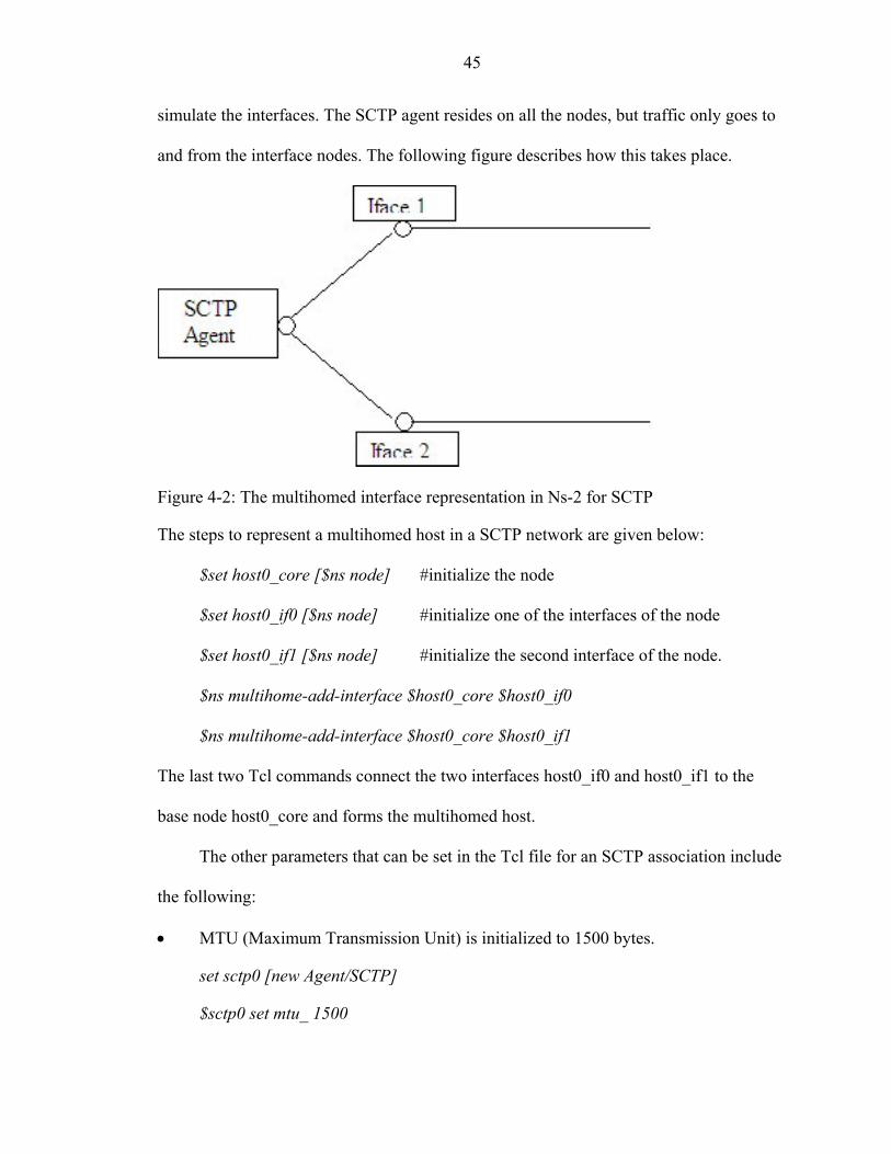
45
simulate the interfaces. The SCTP agent resides on all the nodes, but traffic only goes to
and from the interface nodes. The following figure describes how this takes place.
Figure 4-2: The multihomed interface representation in Ns-2 for SCTP
The steps to represent a multihomed host in a SCTP network are given below:
$set host0_core [$ns node] #initialize the node
$set host0_if0 [$ns node] #initialize one of the interfaces of the node
$set host0_if1 [$ns node] #initialize the second interface of the node.
$ns multihome-add-interface $host0_core $host0_if0
$ns multihome-add-interface $host0_core $host0_if1
The last two Tcl commands connect the two interfaces host0_if0 and host0_if1 to the
base node host0_core and forms the multihomed host.
The other parameters that can be set in the Tcl file for an SCTP association include
the following:
• MTU (Maximum Transmission Unit) is initialized to 1500 bytes.
set sctp0 [new Agent/SCTP]
$sctp0 set mtu_ 1500
46
• Data chunk size of a SCTP packet is initialized to 1448 bytes.
$sctp0 set dataChunkSize_ 1448
• The number of outbound streams is initialized to one each both at the sender and the receiver end.
$sctp0 set numOutStreams_ 1
• The Heartbeat interval is set at one second. This is the interval when the HEARTBEAT chunks are sent.
$sctp0 set heartbeatInterval_ 1
• The initial Receiver window is initialized to 131072 bytes with the option of using the Delayed SACKs on. Delayed SACKs is the mechanism where the receiver waits to piggy back the SACK on top of the data chunks going towards the sender, instead of sending the SACK immediately.
$sctp1 set initialRwnd_ 131072
• The primary path of communication is established at the simulation start up, in the case of a multihomed association.
$sctp0 set-primary-destination $host1_if0
We look at the details of the simulation setup in the next section.
4.2 Simulation Setup
4.2.1 Configuration of the Test Bed
Testing was carried out on the Linux machines of CISE. We have 2 peers named
peer 0 and peer 1. Nodes named 1 and 2 are the multi-homed endpoints of peer 0.
The tests are written using the TCL/TK suite to interact with Ns-2. In the TCL test file,
we can set the various parameters such as the size of the MTU (Maximum Transmission
Unit), the size of the SCTP data chunk, the number of streams in the association, etc., as
discussed in the previous section.
In our test cases, the MTU of the paths is set to 1500 bytes, the data chunk size set
to 1448 bytes and the flag to use Delayed SACK is turned on. Delayed SACK is an
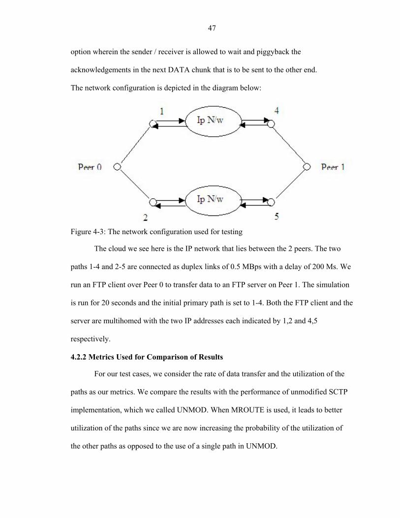
47
option wherein the sender / receiver is allowed to wait and piggyback the
acknowledgements in the next DATA chunk that is to be sent to the other end.
The network configuration is depicted in the diagram below:
Figure 4-3: The network configuration used for testing
The cloud we see here is the IP network that lies between the 2 peers. The two
paths 1-4 and 2-5 are connected as duplex links of 0.5 MBps with a delay of 200 Ms. We
run an FTP client over Peer 0 to transfer data to an FTP server on Peer 1. The simulation
is run for 20 seconds and the initial primary path is set to 1-4. Both the FTP client and the
server are multihomed with the two IP addresses each indicated by 1,2 and 4,5
respectively.
4.2.2 Metrics Used for Comparison of Results
For our test cases, we consider the rate of data transfer and the utilization of the
paths as our metrics. We compare the results with the performance of unmodified SCTP
implementation, which we called UNMOD. When MROUTE is used, it leads to better
utilization of the paths since we are now increasing the probability of the utilization of
the other paths as opposed to the use of a single path in UNMOD.
48
4.2.3 Testing Procedure
We run two test cases here, one with the UNMOD SCTP and the other with
MROUTE SCTP. We transmit data until the 20-second simulation terminates. We then
take into account the rate of data transmission from both the cases. The throughput we
measure here would be the number of data segments we are able to transmit in a given
amount of time (20 seconds) or in other words the number of bytes transmitted per
second.
4.3 Implementation of MROUTE
As discussed in the previous chapter, we add code to the RttUpdate function to
change the current active path if the RTT of any other path was found to be lesser. The
information about each destination such as its IP address, port, cwnd, retransmission
timeout value etc., is stored in a structure SctpDest (Please refer to Appendix-A for the
definition of the structure). If a peer has multiple IP addresses, each of the destinations
would be represented by an instance of SctpDest. All the destination paths of a peer, in
the case of multihoming, would be chained in a linked list, where each node would be an
instance of SctpDest.
We implement the concept of multirouting using the following algorithm.
• Traverse the linked list of the SctpDest structures.
• Record the destination with the lowest RTT.
• If the current active destination path is not the one found with the lowest RTT, then switch the path to this new path by calling the function SetPrimary(). (SetPrimary() sets the current active path to the new destination path that it takes in as a parameter.
We implement the above algorithm in the function RttUpdate() as discussed earlier.
Thus in RttUpdate(), we make use of the available RTT information of all the destination

49
paths including the updated RTT of the path for which RTTUpdate() was actually called.
The MROUTE is implemented after the RTT is updated for the path for which the
RTTUpdate() was called for. The further details about RTTUpdate and the different
structures can be found in the appendix.
4.4 Comparison of MROUTE and UNMOD
In the case of UNMOD SCTP, the user explicitly specifies the primary path to be
used for communication and that remains primary until the simulation ends. But in the
case of MROUTE SCTP, the protocol makes the change of path transparent to the user,
depending on the RTTs of the different paths. Hence the path that the user sets as the
primary path as a part of the configuration set up, may not be the path used during all
times of the simulation. The times we mention in the explanation below represents a
particular instant in seconds of the 20-second simulation. In our test cases, the 1-4 path is
the primary path and 2-5 path is the standby path to begin with. The different stages of
the 20-second simulation of MROUTE and its contrast with UNMOD are enumerated
below:
• In MROUTE, transmission of segments continues in the normal manner along the path 1-4 until the point where the RTT of path 1-4 (which is the primary path to start off with) happens to be longer than the standby path 2-5. At this point (5.704s) the primary path changes to 2-5.
• The new path 2-5 becomes the primary path and all transmission from this point will continue from this point onwards along this new path. The change of path happens twice in the 20-second simulation, once at 5.7s and the other at 10s.
• Though the path has changed, all the segments that had been transmitted along path 1-4 have not yet reached the final destination 4 and are still on their path. SACKs will acknowledge these segments and the ones that have reached the destination. The SACKs will be sent along the 4-1 path to the endpoint 1 of peer 0.
• The path 2-5 is initially in Slow Start. Hence it can send only a maximum of 3 segments, since the initial congestion window, cwnd of the 2-5 path begins with two SCTP segments.

50
• The size of the SCTP Header is 12 bytes and size of the IP Header is 20 bytes. Hence the size of an SCTP segment = 1500(Path MTU) – 12 – 20 = 1468. Since the initial size of cwnd is set at two SCTP segments, it is equal to 1468*2 = 2936 bytes.
• According to the implementation of SCTP, the sender can exceed cwnd by upto (MTU –1) bytes on a new transmission if the cwnd is not currently exceeded. Therefore it is possible to send upto three SCTP segments.
• We find from the simulation results that segments until TSN (Transmission Sequence Number) 162 are sent along 1-4 and from 163 onwards along 2-5. This is shown in the figure 4-4.
1 1.0 1.0 1 2 3 1.75 HB-ACK 3.0 3.0 HB-ACK 5.0 116 5.0 5.0 5.7 162 5.7 5.71 5.74 5.74 163 120 165 162 6.5
Peer 0 Peer 1 Peer 1 Path 1 - 4 Path 2 - 5
TSN of chunks
indicated on the arrows
The numbers along the line indicate the time in seconds
Path Change from 1 –4 to 2 - 5
Figure 4-4: A part of the timeline of the 20-second simulation of MROUTE SCTP.
In Fig 4-4, the peer 1 is unfolded to make the representation of multi-homing
clearer. The numbers along the vertical lines indicate the time elapsed from the start of

51
the simulation. The peer 1 on the left indicates the path of communication as 1 – 4,
whereas the peer 1 on the right indicates the path of communication as 2-5. As we can see
from the diagram, segments till 162 are sent along 1-4, and at time 5.74, peer 0 receives a
HEARTBEAT ACK from the other IP address of peer 1 indicating that the path 2 – 5 is
of a lesser RTT compared to path 1 – 4. Till then, path 2 – 5 was used as a standby path
to measure the Heartbeat measurements along the path 2 – 5.
We can see from the diagram that when the change of path takes place, peer 1 has
only received till segment 120 and peer 0 has received only SACK 116. The other
segments (121 – 162) are still on their way to peer 1 along 1 – 4 path. This also means
that these segments will be SACKed along the path 1 – 4 though the primary path is now
changed to 2 –5. We continue our analysis in the following steps:
• According to the slow start algorithm, SCTP increments cwnd by utmost SMSS (Sender Maximum Segment Size) bytes for each ACK received that acknowledges new data.
• Since the new path along 2-5 is in slow start, it does not increase the cwnd size of 2-5 until it receives SACKs for new segments transmitted along 2-5. Meanwhile the SACKs continue to come along the 4-1 path. These SACKs decrease the flight size and increase the cwnd of the path 1-4, but do not affect the cwnd of the new path 2-5. So actually if we had stayed on the path 1-4, it would have been possible to send more data along 1-4 (which is precisely what happens in the UNMOD as it has already sent many more data segments along 1-4 at this point in simulation).
• To cite an example of the contrast, segment with TSN 166 (the 1st segment along 2-5 after the initial 3 segments are sent) is transmitted at time 6.16s, whereas the same segment with TSN 166 gets sent at time 5.79s in the case of UNMOD SCTP. Graphs showing the difference in the transmission times of segments are shown in the next chapter.
• When the segments reach destination 5 along the path 2-5, the destination 5 realizes that it has received a segment that was expected much further in the future since the earlier segments have not reached 4 (owing to a lower RTT). So it starts sending GAPACKS along 5-2 to indicate the receipt of out-of-order segments.
• LimitMissingReports is a state variable that is maintained, to decide when the retransmission of segments would take place. When a peer end receives GAP
52
ACKs indicating the loss of segments, the number of missing reports for that particular segment is incremented. When the number of missing reports for the segment becomes equal to LimitMissingReports, it is marked for retransmisson. The value of LimitMissingReports is initialized to 4.
• Now after the number of missing reports sent along 5-2 in the GAPACKS exceeds four, it triggers fast retransmission along the paths 2-5 for the segments that have not reached 4 yet (which may include the segments with TSNs 120 – 163 which are still be on their way).
• According to the default behavior of the protocol, retransmission takes place along the path on which the GAP ACK was received (i.e., the path that was not used for the original transmission). In this example the fast retransmission happens along the 2-5 path. When fast retransmission occurs, the ssthresh and cwnd get affected according to the congestion rules of SCTP.
• All the segments marked for retransmission are sent along 2-5 before any new segments are sent along 2-5. All the space in the congestion window created by SACKS along 2-5 is now used up for retransmission, which causes further delay in the delivery of new segments.
• The delay can be further seen in the transmission of TSN 170 (which is the first new segment transmitted along 2-5 after all retransmissions end). In MROUTE it takes place at 6.66s,whereas in UNMOD SCTP it takes place at 5.88s.As we can see, retransmissions and congestion behavior are responsible for a loss of about 0.8 seconds.
• Another problem evident is that the retransmission creates many duplicate segments at the receiver end when the original segments reach the destination along with the retransmitted segments. When the receiver receives the duplicate segments, they send back SACKS containing duplicate TSNs, which on receipt by the sender (peer 0), do not help in increasing the cwnd for the path 2-5. Again time is wasted in waiting for the SACK of non-duplicate segments along 2-5 in order to increase the cwnd or decrease the flight size to facilitate the sending of new data segments along the new path 2-5.
• After this phase of retransmission and duplicate ACKs, transmission of new data segments starts again along 2-5. Ultimately the number of outstanding bytes along 1-4 reduces to 0 as the destination has acknowledged all the segments received along the 1-4 path. The lower RTT of path 2-5 is now used in catching up with the transmission rate of the unmodified.
• However if lower delay persists on path 2-5, we eventually succeed on sending more data segments.

53
A tabular representation of the TSNs sent at different times in both the UNMOD
SCTP and MROUTE SCTP is also shown below in table 4-1:
Table 4-1: Comparison of the time taken to transmit segments in UNMOD and MROUTE.
TSN UNMOD MROUTE 1 1.3 1.3 5 1.75 1.75 10 2.19 2.19 50 3.67 3.67 100 4.46 4.46 150 5.411 5.411 160 5.64 5.64 162 5.69 5.69 163 5.74 5.74 165 5.79 5.74 166 5.79 6.16 170 5.88 6.66 200 6.59 7.51 250 7.73 8.38
• As shown in the table, time gained by the lower RTT of the new path is lost to the
retransmission and the duplicate Acks, thus leading to a lesser rate of transmission than the UNMOD SCTP.
• As the transmission now continues along the path 2-5, the RTT of path 2-5 ultimately becomes greater than the now dormant 1-4. This again leading to a change of the primary path to 1-4. As a result, the change of path again happens at time 10s.
• After the change of path happens for a second time, it exacerbates the situation due to the same problems as before. In the end we find that the modified version is never able to make up for the time lost. We finish the 20-second simulation with the transmission of segment number 776 in the unmodified version and segment number 723 in the modified MROUTE SCTP.
4.5 Problem Analysis and Solutions
In the previous chapter, we had presented a summary of the problems that we faced
in MROUTE and the remedies suggested in the form of a table. In this section, we
mention and elaborate on the categories of problems that we faced in MROUTE along
with proposed solutions. The categories of the problems are listed below:

54
1. Initial Cwnd Problem: The initial value of the cwnd of the new path determines how many segments are transmitted initially.
2. Retransmission problem: As we saw in the analysis of our results above, retransmission of segments due to segments on the new path reaching the destination before earlier transmitted segments, consumes significant time and network resources.
3. Cwnd growth: After we follow one of the solutions that we list for the Initial Cwnd category, it is very important to realize that the growth of cwnd from that point on, affects the rate of data transmission.
4. Oscillation: Basically this problem arises due to the occurrence of too many path changeovers in a given time and may bring about instability in the system.
Each of the classes of the problems and their solutions are discussed next with the
results of MROUTE and UNMOD simulations in context.
4.5.1 Initial Cwnd
From our experiment so far, we find that the initial cwnd of the new path is a
problem. The default value of the initial cwnd as hard-coded in the SCTP protocol is 2
SMSS (Sender Maximum Segment Size), i.e., 2936 bytes. There is a loss of time initially
when the change of path happens to a new path. The SACKs keep coming along 1-4 for
segments sent before the change over was affected. These SACKs decrease the flight size
(the outstanding bytes without acknowledgement) making it possible to send more data
along 1-4. But the cwnd of 2-5 is not affected until the first SACK acknowledging the
first segment transmitted along 2-5 arrives at 2.
Just as an example, in the MROUTE version TSN 166 is the first segment
transmitted along 2-5 after the SACK acknowledging TSN 163 (the first segment sent
after change of path) arrives at 2. TSN 166 is transmitted at time 6.1677s, whereas in the
UNMOD version, TSN 166 is transmitted at time 5.790624s.

55
Thus our goal here is clearly to start somehow with a larger cwnd so that the
transmission of new segments is not affected by the initial size of the congestion window.
We look at three possible ways to handle this:
• Default: Here nothing is done and the default behavior of UNMOD SCTP is retained.
• Using cwnd from the old path: When the change of path takes place, we use the cwnd of the old path for the new path.
• Using history: Use the values of (cwnd, RTT) to predict the cwnd of the new path based on its RTT.
4.5.1.1 Default
Here the existing SCTP implementation is not changed. In the current unmodified
SCTP stack (UNMOD), the size of the initial cwnd is 2 SMSS (Sender Maximum
Segment Size) by default.
4.5.1.2 Using Cwnd from the Old Path
This solution recommends using the current value of cwnd of the old path as the
cwnd of the new path when the change of path takes place to a new path.
Advantages
• We would be starting the cwnd at a value higher than the default of 2 SMSS, which allows us more room to transmit new segments along the new path 2-5.
• This method would tend to follow the behavior of UNMOD SCTP initially since we have room for higher rate of data transmission. Again it depends on how the growth of cwnd is affected after we have an initial value.
Disadvantages
• The 2 paths are not related at all and they have their own delay and congestion characteristics. This could cause problems on the new path.
• The value of the cwnd of the old path is not fixed. If it is high, it will aid us in transmitting new segments. But if the change of path happens very early and the value of cwnd happens to be low, we are again faced with the same problem of less

56
cwnd space for new segments. We can at least be assured that this would be not lead to worse results than the default case.
4.5.1.3 Using History
Here values of pairs of cwnd and delay parameters for the paths are collected and
accordingly predicted as to what the appropriate value of the cwnd should be. We then
start with this value of cwnd as a value for the new path. We could be conservative here
by tweaking the parameters to suit our needs.
Advantages
• We could get a very accurate value of the starting cwnd as we have arrived at this figure from a series of previous observations based on the delay characteristic.
Disadvantages
• There is an added level of complexity and overhead involved in the collecting and storing of the values, calculation and arriving at the new value of cwnd for the new path.
• Again we could be wrong, as there may not be a great deal of co-relation between the delay (RTT) and cwnd.
4.5.2 Retransmission
From our experiment we see that a lot of time gets consumed in the retransmission
of the segments. This retransmission happens due to the GAP ACKS generated by the
receiver. The GAP ACKs are generated because some of the segments that were
transmitted along the old path (1-4) have not reached the destination yet and it has
already received the new segments (segments with higher sequence numbers than
expected) along the new path (2-5). Let us look at some of the proposed solutions to
avoid the loss of time and waste of resources due to retransmission and duplicate
segments.
• Default: As before we do not do anything to stop the retransmission and duplicate segments. Thus we maintain the default behavior of UNMOD SCTP.
57
• Ignore GAP ACKs: The idea here is to ignore GAP ACKs generated by the receiver to allow enough time for the originally transmitted segments along the old path to reach the destination.
• Preventive Retransmission: In this solution, immediately after the change of path takes place, the unacknowledged segments along 1-4 are retransmitted along 2-5 to prevent the GAP ACKs and retransmission at a later point of time.
• Receiver stops GAP ACKs: In order to prevent the retransmission, the receiver stops sending the GAP ACKs to the sender until it receives the originally transmitted segments along the old path.
4.5.2.1 Default
Here we proceed with the default behavior of UNMOD SCTP that does not do
anything to prevent the loss of time due to the retransmission and duplicate segments.
4.5.2.2 Ignore GAP ACKs
We could ignore the GAP ACKs that are generated along the 5-2 path for some
fixed time. The duration of time for which GAP ACKs could be ignored is determined by
considering factors like delay and variance of delay between the two paths on adding the
traffic and on reducing the traffic respectively.
We could also ignore the GAP ACKs until the original segments transmitted
along the old path have reached the destination. Thus we record the last TSN generated
along the old path and predict the time when the last segment would reach the destination
based on the value of RTT we have for the new path. Since the RTT of the old path
changes dynamically, we also update the time when this segment would reach the
destination based on the latest RTT. If we do not keep updating the time, we may be
using an estimated time, which may actually be longer (in which case we are ignoring
GAP ACKS for little too long) or shorter.
But on receiving the GAP ACKs along the new path we would still update the
window values and other RTT estimators for the new path. Fast Retransmission is

58
triggered when the number of GAP ACKs reporting missing segments reaches the upper
bound, LimitMissingReports. Now every time we receive the GAP ACKs along the new
path 2-5, we would have to increase this limit LimitMissingReports in order to prevent
retransmisison. Of course LimitMissingReports has to be increased to a value such that it
is directly proportional to the time taken by the last segment transmitted along the old
path to reach the destination. Since the RTT values are known for each path, we estimate
of the time when the last Data TSN transmitted along the old path would reach the
destination and the ACK returned. But when we receive GAP ACKs along the old path 4-
1, then we do nothing and follow the default behavior.
When a GAP ACK block is received along the new path complaining of the
missing segments, we check if the time has elapsed for the last segment to get to the
destination along the old path and for the sender to receive the SACK (depending on the
RTT). If the time has not elapsed, we increase the LimitMissingReports by one for every
GAP ACK received along the new path. We take care to see that we do not increase
LimitMissingReports for GAP ACKs received along the old path. We cease incrementing
once the time has elapsed and let it retransmit the missing segments along the new path
based on the new value of LimitMissingReports. This method gives enough time to avoid
retransmission. In almost all cases, this time is enough for the segment to reach the other
end and avoid retransmission.
Advantages
• This method is logical in allowing enough time for the last segment along the old path to reach the destination.
• We could think of a situation when the segments actually get lost, i.e., the original segments sent along 1-4 could have actually gotten lost and that the receiver is desperately trying to get the sender’s attention to get it to retransmit. But if our

59
sender is now ignoring GAP ACKs, so there is no way it will know for that fixed time when it is in ‘Ignore’ mode. This is not a problem because if it is a reliable stream the sender will ultimately come to know of the missing segments as soon as it snaps out of it’s ‘ignore’ mode (when the time elapses). Hence ultimately the sender will come to know of the missing segment a little later and retransmit a little later. However the argument in our favor is that we prevent the retransmission and increasing the rate of transmission at an expense of a later retransmission. But even in the worst case of lost segments, retransmission does take place though a little later and segments don’t get lost all that often on a reliable network.
Now in the case of unreliable stream (which is also supported by SCTP), this is not a problem, as SCTP will deliver out of order to the application despite the loss of segments. So this solution works favorably even in the case of actually lost segments.
• We are also preventing the time lost due to the unnecessary duplicate
acknowledgements that are generated when both the original and retransmitted segments reach the destination.
Disadvantages
• As mentioned before, we could be ignoring GAP ACKs for a little more than required or a little less than the required time, which could prove detrimental. If ACKs are ignored for less than the required time, it may lead to faster retransmission that we are trying to avoid.
• In the worst case of lost segments and if we are ignoring GAP ACKs for longer then the required time, please see explanation (ii) of the advantages in this section.
4.5.2.3 Preventive Retransmission
This solution recommends that as soon as the change of path takes place, instead
of transmitting new segments along the new path, retransmit all the segments for which
we have not received SACKs along the old path. Only after these segments are
retransmitted along the new path, will the transmission of new segments take place. As a
result we are preventively taking care to avoid retransmission in the future.
Advantages
• GAP ACKs and thus retransmission are avoided in the future along the new path.

60
• Based on the RTT of the paths, we calculate which segments would have reached the destination before the first segment on the new path and retransmit the rest of the segments. Hence it is a selective retransmission process.
Disadvantages
• We are actually spending time in redundantly retransmitting segments though we might save some time in receiving GAP ACKs and then perform the act of retransmission.
• This still does not eliminate the problem of duplicate acknowledgments generated by the receiver, which prevent an increase in cwnd.
• It may be a little too early to preemptively retransmit the segments; moreover we are again faced with the space in the cwnd to let us retransmit the segments.
• To prevent the duplicate ACKS, additional complexity may be required in the receiver side to prevent the sending of SACKs along the new path for those segments already received on the old path.
4.5.2.4 Receiver Stops GAP ACKs
The receiver could stop sending GAP ACKs for certain duration of time until it
receives the earlier transmitted segments along the old path.
Disadvantages
• Violates the basic rule of the protocol in not transmitting GAP ACKs when it finds missing or out-of-order segments.
• The change of path is transparent to the receiver. Hence it is difficult for the receiver to maintain this state information for something of which it is not aware.
4.5.3 Cwnd Growth
We have talked about the proposed solutions to the initial value of the cwnd of the
new path. This section discusses how the cwnd has to increase in the case of the new
path. We already know that we are handicapped by the initial value of cwnd. Even after
the proposed solutions for the starting value of the cwnd of the new path are followed, we
could still be in trouble after a short period of time when this value is used up. In this

61
section, we search for such a solution that would affect the cwnd uniformly when SACKs
are received, no matter what the starting value of cwnd is.
We look at the following solutions: • Default: The default behavior of SCTP is retained.
• Increase cwnd of old path depending on SACKs along old path.
4.5.3.1 Default
As usual, we do not do anything special and follow the default behavior, which is,
to affect the cwnd of only that path along which the SACKs are received.
4.5.3.2 Increase Cwnd of New Path Depending on SACKs along Old Path
Here we affect the cwnd of the new path 2-5 when we receive the SACKs along
the old path (1-4). In other words we follow the same procedure used to affect the cwnd
of the old path. When there are newly acknowledged bytes in the GAP ACKs received
along the old path, we increment the cwnd of the old path accordingly and decrement the
flight size of the old path. In this solution, we propose that in addition to affecting the
cwnd of the old path, we also carry out this operation for the new path. Thus in response
to ACKs for newly acknowledged segments along the old path, we increment the cwnd of
the new path. Hence we are not contrained by the cwnd of the new path when we do not
receive SACKs along it for a long time.
Advantages
• This could be the most critical of all the solutions that are discussed as we finally see a way of increasing the cwnd of the new path uniformly. This could eliminate the problem of cwnd that we have been facing all along.
• Useful in eliminating the bottleneck preventing the transmission of new or retransmitted segments, ultimately yielding a faster rate of transmission.

62
Disadvantages
• The greatest disadvantage could be that we are affecting the cwnd of a path that is not related in any way to the other path. Thus the cwnd growth may be falsely motivated and artificial.
• This growth of cwnd may make the value reach ssthresh quicker than usual thus leading to premature congestion avoidance.
Comments
We are aware that this problem of cwnd would always be a constraint on the
transmission of data. Even if the seemingly artificial growth of cwnd may lead us to
congestion avoidance phase sooner than expected, it is important to realize that we
reached this stage after transmitting the segments legally on the new path and not
otherwise. Moreover this has given us increased rate of transmission of data segments
and eliminates the wait for SACKS of newly transmitted data. So on the whole this seems
like a solution we should definitely exploit.
4.5.4 Oscillation
As mentioned before, if there are too many changes of path, the system will tend
to oscillate and instability will result. Thus we need to introduce damping as a solution
that prevents the change of path if there is no advantage gained in the long run. If we
determine that a particular change of path will yield minimal benefits and significant
overhead, it is better off to stick to the old path. Only if significant advantages as
compared to the overhead are visible, should a path change be encouraged. We are
currently still investigating analytical methods to detect if a change of path should turn
out in our favor at the end of the simulation or not.

63
4.6 Key Points to Remember
In this chapter, we have discussed the basics of Ns-2, the simulation setup, the
different issues of MROUTE and suggested various categories of alternatives, their pros
and cons. In the previous chapter, we looked at the matrix of the solutions that we have
discussed so far. We have not been able to implement and test all of the combinations
listed. The next chapter talks elaborates implementation and the results obtained from a
few of the important combinations of the solutions namely IGNORE and INC.

CHAPTER 5 IMPLEMENTATION AND ISSUES OF MROUTE VARIATIONS
The previous chapter gave an introduction to the design and implementation of
MROUTE. It also went on to discuss the problems with this implementation and
suggested various solutions to overcome them. We also came up with a matrix
representation of the solutions in chapter 3. This chapter discusses about the
implementation and the results of a few of the solutions such as IGNORE and INC that
we listed. Thus we show that ultimately we are able to achieve the highest rate of data
transmission among all the methods implemented.
5.1 Tabular Representation of Solutions
We again present the matrix of the solutions from chapter 3, below:
Table 5-1: A tabular representation of the solutions. Initial Cwnd Retransmission
Method Path Change (Y / N)
Default(1)
Hysteresis Value
Old-path
Default Preventive Retransmission
Ignore GAP
ACKs UNMOD N × × MROUTE Y × × IGNORE Y × ×
INC Y × × CwndOLD Y × × Or × Cwnd Growth
64
Method
Path Change (Y / N)
Default Use SACKs to increase cwnd
UNMOD × MROUTE × IGNORE Y ×
INC Y × CwndOLD Y × Or ×

65
We have named the different combinations of the solutions that we have tried out
as UNMOD, MROUTE, IGNORE and INC. As indicated in the table, the cross symbol
(×) shows the combination of options that we tried out for each of the methods. As we
can see, the multiroute column tells us whether the multirouting feature is implemented
for that particular solution. All the solutions except UNMOD (unmodified SCTP) are
implemented with the multiroute feature.
As we can see from the table, starting from MROUTE, more options are added as
we progressively advance to the next solution. For instance, in IGNORE, we use the
option of ignoring GAP ACKs for the retransmission category and follow the default
behavior in the ‘cwnd growth’ category. But in INC, we retain the solution of IGNORE
in the retransmission category and also use the segments from the old path to increment
the cwnd of the new path in the ‘cwnd growth’ category.
All the combinations of the options have not been implemented. But the most
critical of the combinations have been implemented and more importantly we have been
able to achieve the goal of higher rate of transmission.
UNMOD is the unmodified SCTP protocol and MROUTE is the naïve
implementation of the multiroute. UNMOD and MROUTE have been discussed and
contrasted in the previous chapter. We will now discuss the implementation issues and
results of IGNORE and INC.
5.2 Design and Implementation of IGNORE
As seen from the table, IGNORE follows the default options in the initial cwnd
and cwnd growth categories. But in the retransmission category, IGNORE chooses to

66
follow the alternative of ignoring GAP ACKs. Let us discuss the details in the further
paragraphs.
When segments are transmitted, they are stored in the SendBuffer till the other
end acknowledges them. The information about each segment such as number of missing
reports, whether it has been GAP ACKed, whether it needs to be retransmitted and other
information. The structure SctpSendBufferNode_S is responsible for storing all this
information about a segment. The SendBuffer is basically a linked list of the
SctpSendBufferNode_S structures. The elements of the structure are further discussed in
detail in the appendix.
LimitMissingReports is a state variable that is maintained, to decide when the
retransmission of segments would take place. When a peer end receives GAP ACKs
indicating the loss of segments, the number of missing reports for that particular segment
is incremented. When the number of missing reports for the segment becomes equal to
LimitMissingReports, it is marked for retransmisson. Retransmission of the segment
takes place whenever it is permitted by cwnd of the path. The idea of ‘Avoiding
retransmission by ignoring GAP ACKs’ is implemented by increasing
LimitMissingReports when a GAP ACK is received in a SACK, in order to delay
retransmission. We keep incrementing LimitMissingReports till the last data TSN sent
along the old path reached the destination.
When a change of path happens, the time when the last segment was sent along
the old path, is recorded. Whenever a GAP ACK block is received, it is checked whether
the time has elapsed for this last segment to reach the destination and get SACKed along
4-1. If the time has not passed, then we increase LimitMissingReports by one. We cease
67
incrementing once the time has elapsed and let it retransmit the missing segments based
on the new value of LimitMissingReports.
We use a flag called eManipRequired to indicate that the change of path has taken
place.
The above-mentioned steps are enumerated below in the form of an algorithm:
• a flag eManipRequired is made true once the change of path occurs.
• If there are GAP ACKs in the SACK chunk,
then if eManipRequired is true
then if CurrentTime < TimeToReach LimitMissingReports++ else eManipRequired = false else LimitMissingReports = 0
ProcessGapAckBlocks() else If CurrentTime > TimeToReach EManipRequired = false;
end if
CurrentTime indicates the current time, TimeToReach represents the tentative time
by which the originally transmitted segment along the old path (1-4) should have reached
the destination and SACKed back along the old path (1-4). TimeToReach is updated
constantly depending on the current RTT of the path. ProcessGapAckBlocks() is the
function, which processes the GAP ACKs, i.e., updates the various parameters like the
flight size (number of outstanding bytes without being ACKed), cwnd for the received
GAP ACK. This function also marks the segments for retransmission based on the
number of missing reports.
Instead of the checking for TimeToReach, we could have also done it based on the
value of the last TSN i.e., check if the TSN SACKed is equal to that of the last segment
68
sent. But if the segment actually gets lost, then we would be increasing the
LimitMissingReports forever without success. This would need another workaround to
solve this problem.
5.3 Analysis of Behavior of IGNORE
The results of IGNORE will be contrasted with the results of MROUTE and
UNMOD. Fast Retransmission is definitely avoided by this, but as we analyze our results
we find that it still does not lead to a faster data transmission rate. We discuss the salient
points in the analysis below:
• After the segments are retransmitted in MROUTE along 2-5, SACKs for the originally transmitted segments are received along 4-1. But these SACKs happen to be the SACKs for the original segments along 1-4, and NOT in response to the retransmitted segments.
• While transmitting / retransmitting the segments, the details of the segment transmitted / retransmitted are recorded in the SendBuffer. SendBuffer, as the name indicates, represents the buffer at the sender side that saves a copy of the segments transmitted till they are ACKed. Also, the information such as the path along which the segment was sent and the TSN of the segment.
• Hence while retransmitting a segment, the path of the segments along which the retransmission takes place is updated to that of the new path. So we override the previous value with that of the new path. In the scenario shown, we update this value from 1 to 2.
• According to the implementation of the protocol stack, after a SACK is received, the TSN of the SendBuffer is compared to the TSN of the received SACK\and then the values of the state variables like cwnd and FlightSize are updated. Since the segment is now ACKed, it is dequeued from the SendBuffer.
• So effectively we are not able to distinguish in the case of a SACK, whether the SACK was meant for the original transmission or for the retransmission. This has been studied in some detail in [15]. Our observations also support the conclusion that if the sender receives a SACK from the original transmission, the wrong path (i.e., the new path, as that is stored in the SendBuffer) gets credited and the congestion window parameters of the new path are affected. In our example, the 2-5 path gets credited for SACKs that came along 1-4.
• So currently there exists no mechanism where we can distinguish between SACKS for retransmissions and original transmissions. Research is currently underway and

69
the developers of Ns-2 SCTP will include their proposed solution in the next release to overcome this problem.
• From the context of the scenario that we simulate, for every SACK received along 1-4, the flightsize is reduced and the cwnd is increased for the 2-5 path incorrectly.
For example, if the TSN 140 is the last TSN in sequence that has reached the destination along 1-4 and if segment with TSN 160 reaches the destination along 2-5 at a later point of time, then the SACK sent for TSN 160 along 2-5 still contains 140 as the cumulative TSN ACK and 160 becomes a part of the GAP ACK. Since the SACK along 2-5 is not advancing the cumulative TSN ACK received at the Sender side, the cwnd of the path 2-5 is not modified, but only the flight size of the 2-5 path is reduced by SMSS bytes. The flight size is reduced because a segment (with TSN 160) along 2-5 has been received at the receiver end.
• Therefore in MROUTE, when a SACK is received after retransmission along path 1-4 before the SACK along 2-5 for the same TSN, two segments can be transmitted/retransmitted along the 2-5 path. Two segments can be sent because the flight size has been reduced and cwnd increased by SMSS (Sender Maximum Segment Size) wrongly for the path 2-5. And for every SACK with a GAPACK received along 2-5, only one segment can be transmitted/retransmitted because the flightSize is decremented by one segment and cwnd is not affected. The ambiguity in distinguishing between SACKs for retransmitted and originally transmitted segments, that we mentioned earlier is responsible for this.
• Ideally speaking, for a SACK received along 1-4, only the flight size and cwnd of the path 1-4 should be affected. This mis-feature (or a feature depending on how you look at it because it leads to a faster data transmission in MROUTE than IGNORE) helps the MROUTE to actually retransmit all the segments very fast and carry on with the transmission of new segments. Since we prevent the process of retransmission in IGNORE, we are not able to attain this behavior and as high a rate of data transmission as MROUTE.
• We are able to prevent the time consumed due to retransmission and duplicate ACKS in case of IGNORE. But due to the reasons discussed in the above paragraph, while IGNORE waits for SACKS along 5-2 to transmit new segments, MROUTE finishes all the retransmission and starts transmitting new segments.
Figure 5-4 depicts the ambiguity in distinguishing between the SACKs for original and the retransmitted segments.

70
6.2 6.2 169 6.57 6.59 169 6.59 154(ReTxed)
155 6.61 156
157 155(ReTxed) 6.62 158 159 160
Path 1 - 4 Path 2 - 5
Peer 1 Peer 0 Peer 1
SACK of 1-4 mistaken for SACK of Retx and new data sent
ReTx starts here with TSN
The numbers along the line indicate the time in seconds
Tsn numbersare indicated on the arrows
Figure 5-1: Ambiguity in distinguishing between the SACKs for retransmission and original transmission in MROUTE
In this figure we can see the problem of distinguishing between the SACKs for
retransmission and those for the original transmission. This is a snap shot of the SCTP
timeline for MROUTE. In MROUTE, peer 0 is able to transmit up to TSN 169 by time
6.2s as shown. After this, fast retransmission is triggered at 6.59s as soon as the GAP
ACKs received along 2-5 increase the number of missing reports to four. But almost at
the same time, the SACK for the originally transmitted segment with TSN 154 arrives
along 1-4. As Peer 0 is not able to differenciate, it mistakes it for the SACK from the
retransmission and manipulates the cwnd parameters for path 2-5. This enables it to

71
retransmit two more segments. So in this way, most of the segments are retransmitted
without much loss of time in MROUTE.
In contrast, IGNORE avoids the process of retransmission, but because we ignore
GAP ACKs, there is no way a wrong path can be credited due to SACKs on some other
path. So most of the time is spent for SACKs along the new path waiting for
acknowledgement of newly transmitted segments along 2-5.
A tabular representation of the TSNs sent at different times in UNMOD, MROUTE and
IGNORE SCTP is also shown below:
Table 5.2 Comparison of performance of UNMOD, MROUTE and IGNORE. TSN UNMOD MROUTE IGNORE
1 1.3 1.3 1.3 5 1.75 1.75 1.75 10 2.19 2.19 2.19 50 3.67 3.67 3.67 100 4.46 4.46 4.46 150 5.411 5.411 5.411 160 5.64 5.64 5.64 162 5.69 5.69 5.69 163 5.74 5.74 5.74 165 5.79 5.74 5.74 166 5.79 6.16 6.16 170 5.88 6.66 6.59 171 5.93 6.66 6.61 175 6.02 6.71 7.04 176 6.02 6.71 7.04 181 6.12 6.98 7.48 200 6.59 7.51 8.07 250 7.73 8.38 9.211
Observations
In the case of IGNORE retransmission does not take place, and some segments
are transmitted earlier compared to MROUTE. In IGNORE DataTsn 171 is transmitted at
time 6.61,but in MROUTE DataTsn 171 is transmitted at time 6.66. Though we gain a

72
little advantage in transmitting a few segments early, we tend to lose this time that we
gained.
In MROUTE segments of TSNs 175 and 176 are the first two new segments sent
immediately after retransmission and are sent at 6.71s. But in IGNORE since we are not
using the SACKs along 4-1 to our advantage as in MROUTE, we send the same segments
with TSNs 175 and 176 at 7.04041s, nearly 0.3 seconds after the same segments are sent
in MROUTE. In MROUTE though we have spent some time not doing any useful work
in receiving the Duplicate ACKs, it is quite insignificant considering the fact that
IGNORE does not have any problem of Duplicate ACKs (since there was no
retransmission).
As a last example of the accumulation of delay, we see that MROUTE transmits
DataTsn 181 at 6.98s and IGNORE transmits the same DataTsn 181 at 7.48(a 0.5 second
delay). Most of the time IGNORE just waits for SACKs along the 5-2 path.
This delay adds up cumulatively and exacerbates, when the change of path takes place
again around the 10-second mark to path 1-4 in the 20-second simulation run. We finish
the 20 second simulation with the transmission of segment no 776 in UNMOD, segment
no 723 in the MROUTE SCTP and segment no 652 in IGNORE. The reduction in the
rate of data transmission can be clearly observed. IGNORE performs the worst compared
to UNMOD and MROUTE.
From this solution we can clearly see that the limited cwnd growth of the new path
is the single largest problem preventing the faster rate of transmission that we always
anticipated. Now let us see how our next solution INC combined with IGNORE aids in
higher rate of data transmission.

73
5.4 Design and Implementation of INC
As we gather from the table shown earlier, we can see that INC has the default
implementation for the initial cwnd category, implements the IGNORE solution
retransmission category and uses the SACK from the old path to increment the cwnd of
the new path in the cwnd growth category.
We saw in our previous solution IGNORE that in case of retransmission, the cwnd of
another path was credited though the SACK arrived along a different path. Now let us
apply this concept uniformly. In other words whenever a SACK arrives on a path that is
not the primary path and as long as the change of path has taken place at least once, we
credit the cwnd of the current or the primary path. Note that since we are also using the
solution of IGNORE, we do not have the problem of distinguishing between SACKs. In
summary, in addition to reducing the flight size and incrementing cwnd of the path along
which the SACK was received, we also increment cwnd of the primary path. This will
definitely enable us to transmit more data segments along the new path and there will not
be any constraint. We also saw that the crediting of a different path for SACKs along
another path definitely helped in increasing the rate of transmission in MROUTE when
compared to IGNORE.
Much of the implementation is in the function ProcessSackChunk(), which
processes a SACK chunk when received. The main responsibilities of this function
include processing of the GAPACKs if any, decrementing the flight size and
incrementing the cwnd size of the path, if new segments are acknowledged. This is where
we add the code to manipulate the flight size and cwnd parameters of the primary path.
Since we are using the IGNORE solution as a part of INC, we also avoid retransmission
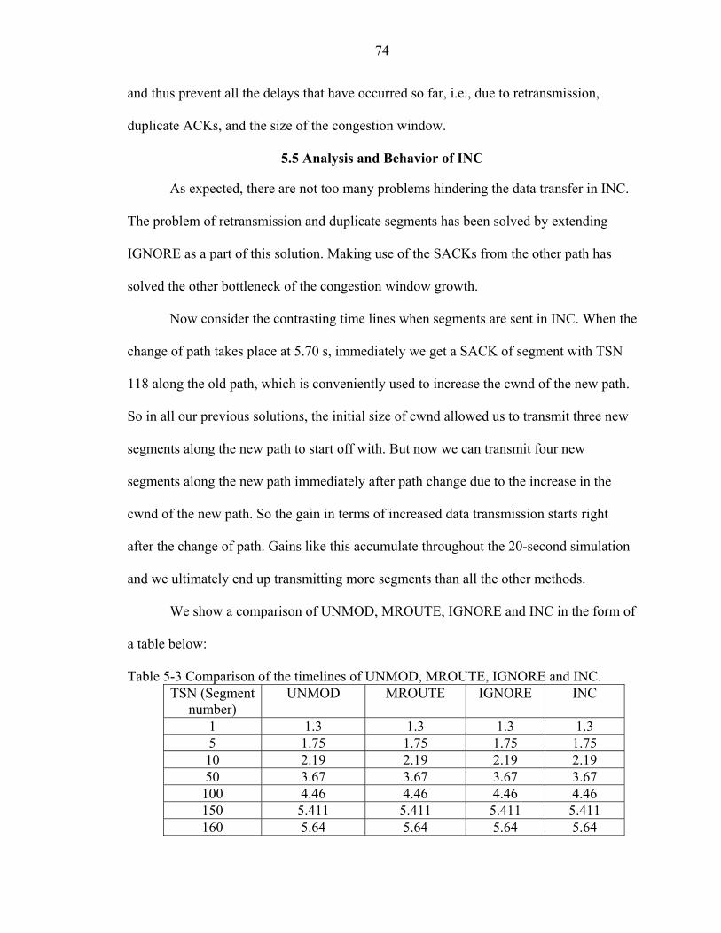
74
and thus prevent all the delays that have occurred so far, i.e., due to retransmission,
duplicate ACKs, and the size of the congestion window.
5.5 Analysis and Behavior of INC
As expected, there are not too many problems hindering the data transfer in INC.
The problem of retransmission and duplicate segments has been solved by extending
IGNORE as a part of this solution. Making use of the SACKs from the other path has
solved the other bottleneck of the congestion window growth.
Now consider the contrasting time lines when segments are sent in INC. When the
change of path takes place at 5.70 s, immediately we get a SACK of segment with TSN
118 along the old path, which is conveniently used to increase the cwnd of the new path.
So in all our previous solutions, the initial size of cwnd allowed us to transmit three new
segments along the new path to start off with. But now we can transmit four new
segments along the new path immediately after path change due to the increase in the
cwnd of the new path. So the gain in terms of increased data transmission starts right
after the change of path. Gains like this accumulate throughout the 20-second simulation
and we ultimately end up transmitting more segments than all the other methods.
We show a comparison of UNMOD, MROUTE, IGNORE and INC in the form of
a table below:
Table 5-3 Comparison of the timelines of UNMOD, MROUTE, IGNORE and INC. TSN (Segment
number) UNMOD MROUTE IGNORE INC
1 1.3 1.3 1.3 1.3 5 1.75 1.75 1.75 1.75 10 2.19 2.19 2.19 2.19 50 3.67 3.67 3.67 3.67 100 4.46 4.46 4.46 4.46 150 5.411 5.411 5.411 5.411 160 5.64 5.64 5.64 5.64
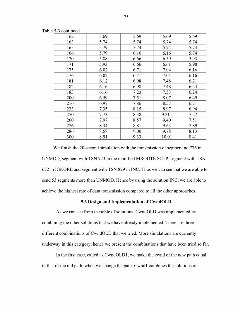
75
Table 5-3 continued 162 5.69 5.69 5.69 5.69 163 5.74 5.74 5.74 5.74 165 5.79 5.74 5.74 5.74 166 5.79 6.16 6.16 5.74 170 5.88 6.66 6.59 5.93 171 5.93 6.66 6.61 5.98 175 6.02 6.71 7.04 6.16 176 6.02 6.71 7.04 6.16 181 6.12 6.98 7.48 6.21 182 6.16 6.98 7.48 6.23 183 6.16 7.23 7.53 6.24 200 6.59 7.51 8.07 6.49 216 6.97 7.86 8.57 6.71 233 7.35 8.15 8.97 6.94 250 7.73 8.38 9.211 7.27 260 7.97 8.57 9.40 7.51 276 8.34 8.81 9.63 7.89 286 8.58 9.00 9.78 8.13 300 8.91 9.33 10.01 8.41
We finish the 20-second simulation with the transmission of segment no 776 in
UNMOD, segment with TSN 723 in the modified MROUTE SCTP, segment with TSN
652 in IGNORE and segment with TSN 829 in INC. Thus we can see that we are able to
send 53 segments more than UNMOD. Hence by using the solution INC, we are able to
achieve the highest rate of data transmission compared to all the other approaches.
5.6 Design and Implementation of CwndOLD
As we can see from the table of solutions, CwndOLD was implemented by
combining the other solutions that we have already implemented. There are three
different combinations of CwndOLD that we tried. More simulations are currently
underway in this category, hence we present the combinations that have been tried so far.
In the first case, called as CwndOLD1, we make the cwnd of the new path equal
to that of the old path, when we change the path. Cwnd1 combines the solutions of

76
MROUTE, IGNORE and INC in addition to making the cwnd of the new path equal to
that of the old path. We present the behavior of CwndOLD1 in the next section.
The behavior of CwndOLD1 influenced the implementation of CwndOLD2 and
CwndOLD3. In CwndOLD2, we made the cwnd of the new path half of the cwnd of the
old path. In other words, cwndnew = 0.5 * cwndold. In CwndOLD3, the cwnd of the new
path was made 0.75 * cwnd of the old path, i.e., cwndnew = 0.75 * cwndold .
But both CwndOLD2 and CwndOLD3 were only tried with MROUTE and not
with any other solution. This means that we let the retransmissions and duplicate
acknowledgements take its natural course. CwndOLD2 and CwndOLD3 were also faced
with limited cwnd growth as before. We discuss the performances of CwndOLD2 and
CwndOLD3 in the next section.
5.7 Analysis and Behavior of CwndOLD
5.7.1 CwndOLD1
The idea in CwndOLD1 is to make the cwnd of the new path equal to that of the
old path when the change of path takes place due to MROUTE. In CwndOLD1, we use
the solutions of IGNORE to ignore GAP ACKs and use INC to increment the cwnd of the
new path based on SACKs from the old path.
The following points summarize the behavior of CwndOLD1 in a simulation of the
same network scenario for 20 seconds:
• The behavior until the point when the path changes, is similar to MROUTE. The RTT of the second path becomes lesser than that of the first path at 5.704s. The cwnd of the old path is now 66,070, as it has already exceeded ssthresh and is in congestion avoidance phase.
• The cwnd of the new path is now made equal to 66,070 according to the implementation of CwndOLD1. This is a rather huge value for the cwnd of the new path to start with.

77
• As the cwnd of the new path is huge, it starts to send a burst of data segments till the cwnd is full. So in the simulation, peer 0 sends segments from TSN 163 till TSN 208 immediately after the change of path.
• Since 45 SCTP segments are initially transmitted in a burst, the RTT of the 2-5 starts to climb and becomes higher than the RTT of the old path 1-4. The RTT of the new path 2-5 becomes higher than the RTT of path 1-4 after 1.7s of usage. The reason for this is the congestion introduced along 2-5 by the sudden burst of data.
• The second change of path happens at 7.4s and then it exhibits the same behavior.
• As we progress, we see numerous path changes in 20 seconds. Some of the path changes take place in as less an interval of 0.02 seconds.
• At the completion of the 20-second simulation, we have about 25 path changes. But at the same time, we are able to transmit upto 937 segments in 20 seconds as opposed to 829 in INC, 776 in UNMOD and 723 in MROUTE.
We now look at the behavior of CwndOLD2 and CwndOLD3 in the following section.
5.7.2 CwndOLD2 and CwndOLD3
In CwndOLD2 and CwndOLD3, we use only the solution of MROUTE and make
the cwnd of the new path equal to one half and three fourths of cwnd of the old path
respectively. Other solutions like IGNORE and INC are not used because we see in the
behavior of CwndOLD1 that having a huge cwnd value leads to a burst of data, that fills
up the cwnd. We do not further want to complicate the value of cwnd by using INC to
increase the cwnd of the new path from SACKs along the old path. For the same reason,
we do not prevent the retransmissions and generation of duplicate acknowledgements by
choosing not to include IGNORE as a part of CwndOLD2 or CwndOLD3.
In CwndOLD2, we make the cwnd of the new path equal to one half of the cwnd
of the old path during the change of path i.e., cwndnew = 0.5 * cwndold. In CwndOLD3, we
make the cwnd of the new path equal to three fourths of the cwnd of the new path during
the change of path, i.e., cwndnew = 0.75 * cwndold. We run the simulation with our
network scenario for 20 seconds.

78
The behavior of CwndOLD2 and CwndOLD3 are summarized below:
• It is similar to the behavior of MROUTE and CwndOLD1 till the point when the change of path takes place. As in the case of CwndOLD1, the cwnd of the old path is is now 66,070, as it has already exceeded ssthresh and is in congestion avoidance.
• The cwnd of the new path is now made equal to 33,035 bytes according to the implementation of CwndOLD2. As this happens to be a big value, but not as big as in the case of CwndOLD1, there is an initial burst of about 20 SCTP segments before the cwnd becomes full.
• In the case of CwndOLD3, we make the value of cwnd equal to 49,552 bytes. Here it leads to an initial burst of about 35 SCTP segments before the cwnd becomes full.
• But since we are not using INC or IGNORE, the cwnd of the new path is not affected in any other way. We find that we are able to transmit upto 765 segments in case of CwndOLD2 and 775 segments in the case of CwndOLD3. We come very close to 776 segments as the case of UNMOD. We also observe that we have actually performed better than MROUTE, where only 723 segments were transmitted.
• We also find that there are only two changes of paths as the case of MROUTE, IGNORE and INC. The system does not become instable as in the case of CwndOLD1.
5.8 Comments on CwndOLD
Though we are able to send about a 100 segments more than INC in CwndOLD1,
it totally shocks the system and leads to oscillations in the system. 25 path changes in 20
seconds are equivalent to more than one path change per second, which brings the system
into instability. We have already talked about the problem of oscillation in the third
chapter.
Thus we need to decide if changing paths will bring oscillation into the system in
the long run. If the overhead of the path changes is more than the benefits we realize in
terms of increased rate of data transmission, we are better off continuing along the old
path. We are currently working on an analytical model to decide if the change of path is

79
significantly beneficial compared to the overheads involved and then decide to change
the path. Thus if we are able to use the analytical solution in deciding when to change the
path and when not to, we will be able to prevent the oscillatory behavior of the system.
In CwndOLD2 and CwndOLD3, though we had the initial burst of data, we did
not have the problem of oscillation and equaled the data transmission rate of UNMOD
and performed better than MROUTE. Hence if we are able to start with the right value of
cwnd for the new path, we will be able to perform better than UNMOD without having to
use IGNORE, INC or other variations of MROUTE. Hysteresis method could also prove
useful here in using information from a previously collected pairs of values of (cwnd,
RTT) of the paths. We discuss the issue of choosing the right value of cwnd in the next
chapter and in the ‘Future-Work’ section of the seventh chapter.
5.9 Key Points to Remember
Since we are still currently doing research in the issues of CwndOLD, we do not
use any of CwndOLD1, CwndOLD2 or CwndOLD3 to compare against MROUTE,
UNMOD, IGNORE and INC. For the same reason, we do not discuss about CwndOLD
or the implementations under it further in this thesis.
With this, all the methods that have been implemented have been explained. From
the experiments so far, we can infer that the size of the congestion window, cwnd, plays a
very important role in the increased rate of transmission. In effect, we have seen that
taking care of the congestion window growth has solved our problems that we had been
facing in our earlier solutions. In the next chapter, we again formally state the results
obtained in the forms of graphs and tables. We also evaluate the results against our earlier
assumed metrics of number of segments transmitted in unit time. In our case, since we
have run 20-second simulations, the unit time for consideration is 20 seconds.

CHAPTER 6 RESULTS AND EVALUATION
In the previous chapters, we have discussed different implementations like
MROUTE (Plain multiroute), IGNORE, INC and CwndOld. We also analyzed the
simulation results of these implementations and how they fared against the unmodified
SCTP, UNMOD. In this chapter, we restate the results that we have already obtained and
compare our results against the metrics that we had assumed earlier.
The setup of the test bed has already been discussed. We considered the number
of segments that we are able to transmit in a given amount of time as the performance
metric. Since we run 20-second simulations, we consider the number of segments or the
number of bytes of data we are able to transmit in 20 seconds, as the metric. RTT (Round
Trip Time) is an excellent measure of the conditions along the path. It is also a good
indicator of the congestion conditions and network traffic conditions along the path. If
there were congestion, then it would lead to a higher RTT. Otherwise it would lead to a
lower RTT. We have based our implementations on mostly the RTT of the path.
We have looked at the analytical results of each of the solutions in the previous
chapters. In this chapter we again discuss the results of the simulation and evaluate it
against the metric chosen.
6.1 Comparison of MROUTE and UNMOD
In MROUTE, we implemented the naïve implementation of the multiroute. In this
implementation, when the RTT of another path was found to be lesser than that of the
primary path, we changed the primary path to the new one. The RTT information from
80

81
HEARTBEAT chunks was used to evaluate the standby paths. We already know the
primary path’s RTT since as data exchange is taking place along that path.
We showed the tabular representation of the timelines during the transmission of
segments in UNMOD and MROUTE in the previous chapter. A graph is presented here
with data taken from the same table.
Comparison of Protocol Performance between UNMOD and MROUTE
0
2
4
6
8
10
1 10 100
160
163
166
200
TSN
Tim
e in
Sec
onds
UNMODMROUTE
Figure 6-1: Graph showing the performances of UNMOD and MROUTE. X-axis
represents the TSN transmitted and Y-Axis shows the time when it was transmitted.
The graph is further explained as below:
• As we can infer from the graph, the performance of UNMOD is the same as MROUTE until the change of path takes place in MROUTE.
• The time gained by the lower RTT of the new path in the case of MROUTE is lost to the retransmission and the duplicate ACKs. This leads to a lesser rate of transmission than the UNMOD.
• After the dust has settled down after the retransmission and the duplicate ACKs, MROUTE starts to gain and catch up with that of UNMOD. This continues for a while and then before there can be further improvement, the RTT of path 2-5 becomes greater than the now dormant 1-4, again leading to a change of the primary path to 1-4. The change of path again happens at time 10s.

82
• After the change of path happens for a second time, it exacerbates the situation due to the same problems as before. In the end we find that the modified version is never able to make up for the time lost. We finish the 20-second simulation with the transmission of segment no 776 in the unmodified version and segment no 723 in the modified MROUTE SCTP.
In UNMOD, we transmit 776 DATA chunks in 20 seconds. The size of each data
chunk is set to 1448 bytes. This gives us the sender transmission rate of (776 * 1448) / 20
= 56.182 KB per second.
We finish the 20-second simulation of MROUTE with segment of TSN 723. This gives a
sender transmission rate of (723 * 1448) / 20 = 52.345 KB per second.
6.2 Comparison of MROUTE, UNMOD and IGNORE
We can conclude from the previous section that the plain MROUTE did not yield
the expected results because of reasons namely the problem of retransmission, duplicate
segment generation and growth of cwnd of the new path. These reasons were elaborated
in the previous chapters.
Therefore in IGNORE, we fixed the problems of retransmission and the
generation of duplicate segments by choosing to ignore GAP ACKS for a duration of
time proportional to the time taken by the last segment transmitted along the old path to
reach the destination and ACKed back.
The graph below show the comparison of performances of UNMOD, MROUTE
and IGNORE. We have already shown the tabular depiction of the timelines of
transmission in the fifth chapter.
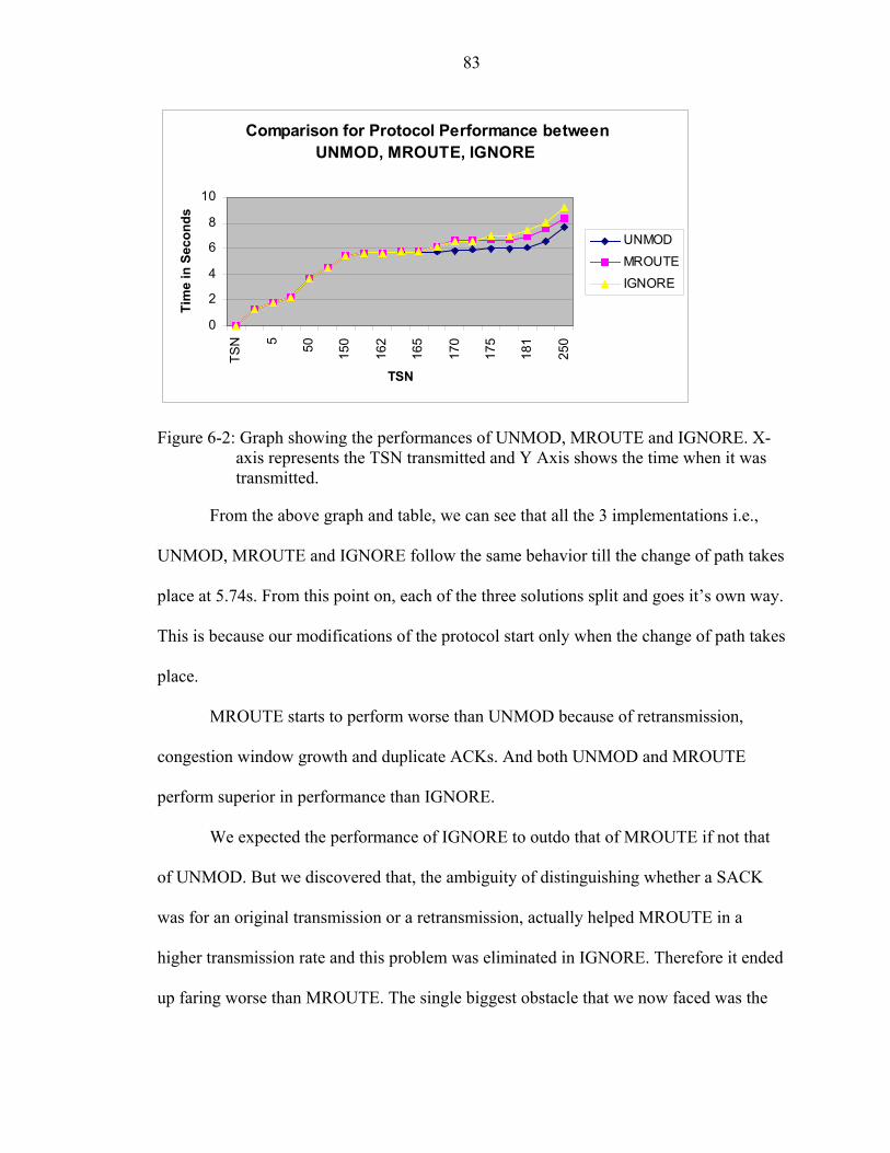
83
Comparison for Protocol Performance between UNMOD, MROUTE, IGNORE
0
2
4
6
8
10
TSN 5 50 150
162
165
170
175
181
250
TSN
Tim
e in
Sec
onds
UNMOD
MROUTE
IGNORE
Figure 6-2: Graph showing the performances of UNMOD, MROUTE and IGNORE. X-axis represents the TSN transmitted and Y Axis shows the time when it was transmitted.
From the above graph and table, we can see that all the 3 implementations i.e.,
UNMOD, MROUTE and IGNORE follow the same behavior till the change of path takes
place at 5.74s. From this point on, each of the three solutions split and goes it’s own way.
This is because our modifications of the protocol start only when the change of path takes
place.
MROUTE starts to perform worse than UNMOD because of retransmission,
congestion window growth and duplicate ACKs. And both UNMOD and MROUTE
perform superior in performance than IGNORE.
We expected the performance of IGNORE to outdo that of MROUTE if not that
of UNMOD. But we discovered that, the ambiguity of distinguishing whether a SACK
was for an original transmission or a retransmission, actually helped MROUTE in a
higher transmission rate and this problem was eliminated in IGNORE. Therefore it ended
up faring worse than MROUTE. The single biggest obstacle that we now faced was the
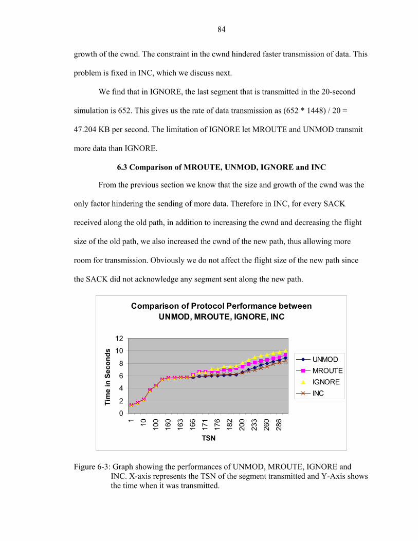
84
growth of the cwnd. The constraint in the cwnd hindered faster transmission of data. This
problem is fixed in INC, which we discuss next.
We find that in IGNORE, the last segment that is transmitted in the 20-second
simulation is 652. This gives us the rate of data transmission as (652 * 1448) / 20 =
47.204 KB per second. The limitation of IGNORE let MROUTE and UNMOD transmit
more data than IGNORE.
6.3 Comparison of MROUTE, UNMOD, IGNORE and INC
From the previous section we know that the size and growth of the cwnd was the
only factor hindering the sending of more data. Therefore in INC, for every SACK
received along the old path, in addition to increasing the cwnd and decreasing the flight
size of the old path, we also increased the cwnd of the new path, thus allowing more
room for transmission. Obviously we do not affect the flight size of the new path since
the SACK did not acknowledge any segment sent along the new path.
Comparison of Protocol Performance between UNMOD, MROUTE, IGNORE, INC
0
2
4
6
8
10
12
1 10 100
160
163
166
171
176
182
200
233
260
286
TSN
Tim
e in
Sec
onds
UNMODMROUTEIGNOREINC
Figure 6-3: Graph showing the performances of UNMOD, MROUTE, IGNORE and INC. X-axis represents the TSN of the segment transmitted and Y-Axis shows the time when it was transmitted.
85
We retained the solutions of IGNORE and MROUTE in INC in addition to the
modification that we just mentioned. The graph above show the comparison of
performances of UNMOD, MROUTE and IGNORE.
Again, all the four methods follow a similar pattern till the change of path takes
place at 5.7s. As expected, INC performed the best of all the methods, i.e., UNMOD,
MROUTE and INC. In the 20-second simulation, we were able to transmit 829 segments,
which is nothing but (829 * 1448) / 20 = 60 KB per second. Thus we are able to gain
more data transmission when compared to IGNORE, MROUTE and UNMOD
respectively.
6.4 Key Points to Remember
We still have not been able to complete all the combinations of solutions given in
the matrix. There is a good deal of research left in the topic of multirouting that one can
do. We are currently investigating the problem of initial size of cwnd, in which one of the
solutions suggested was the hysteresis method. In this method, we collect the pairs of
(RTT, cwnd) for the paths and then make a prediction as to what the cwnd value for a
new path with a particular RTT should be, when we switch to it.
In all the implementations so far, we start with a default size of 2 SMSS (Sender
Maximum Segment Size) bytes. But we have been evaluating the other path for sometime
now, by means of HEARTBEAT chunks before switching over to it. After knowing the
characteristics such as RTT of the path, we should be able to do more than just start the
cwnd of the path with 2 SMSS bytes. We can further corroborate the previous statement
by saying that our prior knowledge of congestion along that path should be used to our
advantage in starting the cwnd of the new path with a higher value.

86
The next (concluding) chapter outlines the summary of the entire thesis and
concludes with the discussion of various research ideas in SCTP, in the Future-Work
section.
CHAPTER 7 CONCLUSIONS AND FUTURE WORK
This chapter summarizes the entire thesis and evaluation of the results. It concludes
with future research topics and activities that can be carried out in the topic of
multirouting and SCTP in general.
7.1 Summary
Initially we started from the proposal that the idea of a single path that remains
active throughout the lifetime of an SCTP association, would not fully utilize the true
multihoming features supported by SCTP [16]. HEARTBEAT chunks are used in SCTP
to periodically check if a particular destination is alive or not. Since these chunks carry
the timing information in them, they can be used to measure the RTT (Round Trip time)
of the paths. From the RTTs that we collect periodically, if the association is multihomed,
we evaluate each of the paths if the association is multihomed. If the RTT of a path
happens to be lesser than that of the primary path, then change of path takes place to the
path of lesser RTT. This was the plain naïve implementation of multirouting, MROUTE.
The simulation tests were run and the results compared against the unmodified version of
SCTP, UNMOD. It was expected that MROUTE would perform better than UNMOD in
terms of better rate of data transmission.
We found that MROUTE actually yielded inferior performance when compared to
UNMOD. The main reasons that resulted in the worse performance were attributed to
retransmission, generation of duplicate ACKs and the constraint in the growth of
87
88
congestion window cwnd. The different solutions and their combinations, advantages and
disadvantages were listed.
To prevent retransmission and generation of duplicate ACKs, a second design,
IGNORE was implemented. IGNORE resulted in prevention of the retransmission and
the generation of duplicate ACKs. It was expected that IGNORE would perform better
than MROUTE. But when the simulation tests were run, it was found that IGNORE
performed worse than both MROUTE and UNMOD. The main reason was that the
growth of cwnd was limited which did not permit new data segments to be transmitted.
A third design, INC which uniformly incremented the cwnd of the new path on
receiving the SACKs from the old path, was implemented. It also combined the IGNORE
design to prevent the retransmission and generation of duplicate ACKs. When this was
tested, it was found that this solution performed the best when compared with UNMOD,
MROUTE and IGNORE. In a given 20-second simulation, INC transmitted more data
segments than any of the other three versions.
To summarize, UNMOD, MROUTE and IGNORE achieved data rates of 56.182
KB/sec, 52.345 KB/sec and 47.204 KB/sec respectively. To top it all, INC attained the
data transmission rate of 60 KB/sec.
We also explained about the performance of CwndOLD. Since we are still in the
experimental stages of this implementation, we did not compare CwndOLD against
UNMOD, MROUTE, IGNORE or INC.
7.2 Future Research
The SCTP protocol is relatively new compared to TCP and older protocols.
Therefore there is scope for a lot of research in SCTP. Most of the problems found in
TCP and their adaptations and versions can be applied to SCTP as well. The features

89
unique to SCTP such as multihoming, message boundary preservation, multiple logical
streams in a single association etc. can be exploited further and tailored to specific
applications. There are a lot of quality research topics that can arise in the area of SCTP.
Some of the interesting topics are listed below:
7.2.1 SCTP in Wireless Networks
There have been many solutions to the problem of adapting the TCP for use in
wireless networks. A few of these are the Indirect TCP [17], Mobile TCP [18] and
Freeze-TCP [19]. The modifications suggested to make TCP adaptable to wireless
networks can also be applied to SCTP.
Handover management is an area of research that is very critical to the functioning
of the wireless networks industry. The ability of the network to support seamless
handover determines the success of real-time sensitive services such as VoIP (Voice over
IP) telephony, video etc. Seamoby [20] is currently a hot research topic and stands for
Seamless Mobility. Work is also currently being done in the topic of context transfer
framework [21], where a context sensitive framework is to be made available to the new
access router from the old access router, for it to continue serving the mobile node with
the same quality constraints as before the handover.
The multihoming feature of SCTP can be used in mobile SCTP where one of the
addresses of the multihomed association would function as the home address and the
other would be the foreign address. So in such a situation, the handovers between these
two addresses during mobility management could be seamless as both the addresses
physically belong to the same device. Not much of research has been performed in this
area.

90
7.2.2 SCTP as a Transport for FTP
FTP (File Transfer Protocol) is most widely used for file transfer across two hosts.
A single FTP connection is actually made of two TCP connections [22]. One of the
connections is a control connection that exists throughout the lifetime of a FTP
association and the other is a data connection that is created when the user issues an FTP
command and is destroyed as soon as the results are fetched. In other words, whenever a
file is to be fetched from the server to the client, a separate data connection is created for
this purpose and then destroyed after the file transfer keeping only the control connection
alive. Since SCTP supports multiple streams in a single connection and has a logical
division of raw data bytes into chunks, the framework of SCTP can be embraced very
naturally to support FTP. One of the streams of the SCTP connection can be used for
control connection and the other can be used for the data connection in a single SCTP
association. Both the control and the data connections of the FTP can be supported in one
SCTP association.
7.2.3 SCTP as a Transport for HTTP
HTTP [23] is one of the most widely protocols used for Internet access. TCP is
currently the transport for the HTTP. SCTP support has not yet been incorporated into
HTTP. Using the SCTP features of multi-homing, one can effectively share the load
while using HTTP/SCTP. Padmanabhan gives an example that transmission of a web
page from a server to a client involves the transfer of distinct components [24]. The
different components could be image data, text data etc.
Thus developing HTTP over SCTP would further enhance the efficiency of the
data transfer by having each SCTP chunk carry one logical component of a website in a
91
single SCTP association. Coupled with true multirouting, we could make the transfer of
each of the components to the destination parallel. This would definitely help in faster
data transmission rather than transferring all the components in a single path.
7.2.4 Achieve True Multirouting
Currently in this thesis, we are providing multiroute support such that only one of
the paths is active at any time. True multirouting can be achieved by making all the paths
of an SCTP association active at the same time. Thus the total data traffic to be
transmitted to the peer end could be distributed over all the paths such that the traffic
along each path is directly proportional to the characteristics of the path such as RTT,
packet loss, congestion etc. An example of a true multihoming application was given in
the previous paragraph where we talked about each of the paths of an SCTP association
carrying separate data chunks as part of a single HTTP connection between the client and
the server. That was an instance of running HTTP / SCTP.
7.2.5 Complete the Matrix
In an earlier chapter, we listed the different combinations of the solutions that we
proposed in a table. However in this thesis, we are not able to provide all the
combinations listed in the table. The future research in this direction would be to
implement more combinations and study the behavior and performance of SCTP.
The other interesting combinations that can be implemented are shown below along
with the solutions currently experimented.

92
Table 6-1: Combinations of solutions for future research Initial Cwnd Retransmission
Method Path Change (Y / N)
Default(1)
Hysteresis Value
Old-path
Default Preventive Retransmission
Ignore GAP ACKs
UNMOD N × × MROUTE Y × × IGNORE Y × ×
INC Y × × × CwndOLD Y × × Or ×
Y × Or × × Y × Or × Or × × Y × × Y × Or × ×
Cwnd Growth
Method Path Change (Y / N)
Default Use SACKs to increase cwnd
UNMOD × MROUTE × IGNORE Y ×
INC Y × CwndOLD Y × Or ×
× Or × × Or × × Or × × Or ×
In the conclusion of the previous chapter, we elaborated on the hysteresis method
in the ‘Initial cwnd’ category. We mentioned that a prediction of the new value of cwnd
could be made when we switch to a path because we have been collecting pairs of (RTT,
cwnd) for other paths and hope this is a good starting value.
We can choose not to be too conservative by starting with slow-start cwnd value
of two SMSS. In a new unexplored path, it is fine to start with slow-start cwnd value,
because we are not aware of the network and the congestion conditions on that path. But
in our case, in the case of a multihomed association, we have details about the standby

93
paths in terms of RTT information by means of the HEARTBEAT chunks. RTT
information is one of the very good indicators of congestion on a path. Hence we could
use this value to our advantage and start with a higher value of cwnd on this path if we
get a lower RTT switch to it. Otherwise we could stick with the default value of cwnd if
we get bad RTT values on it. Good or bad RTT values is again relative and can be
compared with the pairs of (cwnd, RTT) values that we collect for the primary path and
then a decision about the starting value can be taken. Obviously a higher starting value
will permit us to transmit more data segments when we switch to it.
7.2.6 SCTP as Transport for Other Applications
SCTP can be developed as the transport for many other applications currently
using TCP as the transport layer like SMTP, RTP etc. Madisetti talks about the suitability
of SCTP for voice and video applications [25].
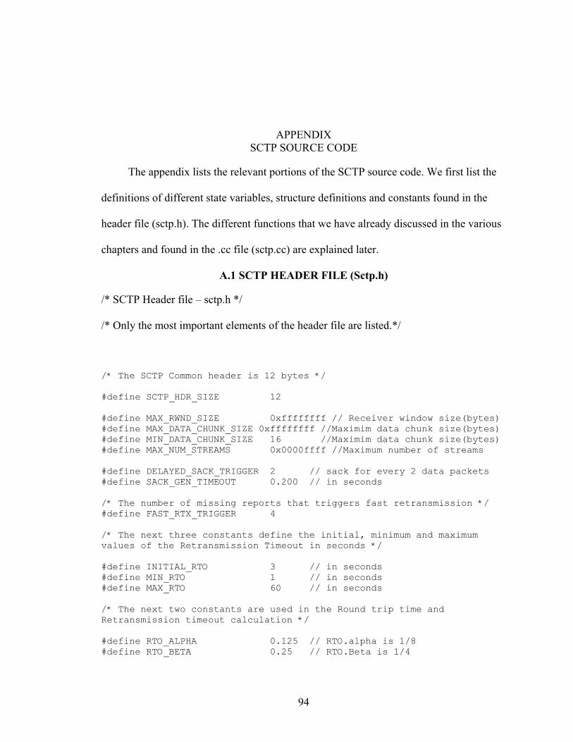
APPENDIX SCTP SOURCE CODE
The appendix lists the relevant portions of the SCTP source code. We first list the
definitions of different state variables, structure definitions and constants found in the
header file (sctp.h). The different functions that we have already discussed in the various
chapters and found in the .cc file (sctp.cc) are explained later.
A.1 SCTP HEADER FILE (Sctp.h)
/* SCTP Header file – sctp.h */
/* Only the most important elements of the header file are listed.*/
/* The SCTP Common header is 12 bytes */ #define SCTP_HDR_SIZE 12 #define MAX_RWND_SIZE 0xffffffff // Receiver window size(bytes) #define MAX_DATA_CHUNK_SIZE 0xffffffff //Maximim data chunk size(bytes) #define MIN_DATA_CHUNK_SIZE 16 //Maximim data chunk size(bytes) #define MAX_NUM_STREAMS 0x0000ffff //Maximum number of streams #define DELAYED_SACK_TRIGGER 2 // sack for every 2 data packets #define SACK_GEN_TIMEOUT 0.200 // in seconds /* The number of missing reports that triggers fast retransmission */ #define FAST_RTX_TRIGGER 4 /* The next three constants define the initial, minimum and maximum values of the Retransmission Timeout in seconds */ #define INITIAL_RTO 3 // in seconds #define MIN_RTO 1 // in seconds #define MAX_RTO 60 // in seconds /* The next two constants are used in the Round trip time and Retransmission timeout calculation */ #define RTO_ALPHA 0.125 // RTO.alpha is 1/8 #define RTO_BETA 0.25 // RTO.Beta is 1/4
94

95
Boolean_E eManipRequired; // used in the IGNORE solution Boolean_E ePathChanged; // To indicate that the path has changed /* To hold the tentative time taken by the segment to reach the destination and get ACKed back */ double TimeToReach; /* SCTP chunk types */ typedef enum SctpChunkType_E { SCTP_CHUNK_DATA, SCTP_CHUNK_INIT, SCTP_CHUNK_INIT_ACK, SCTP_CHUNK_SACK, SCTP_CHUNK_HB, SCTP_CHUNK_HB_ACK, SCTP_CHUNK_ABORT, SCTP_CHUNK_SHUTDOWN, SCTP_CHUNK_SHUTDOWN_ACK, SCTP_CHUNK_ERROR, SCTP_CHUNK_COOKIE_ECHO, SCTP_CHUNK_COOKIE_ACK, SCTP_CHUNK_ECNE, // reserved in rfc2960 SCTP_CHUNK_CWR, // reserved in rfc2960 SCTP_CHUNK_SHUTDOWN_COMPLETE, /* RFC2960 leaves room for later defined chunks */ }; /* SCTP chunk common header structure */ typedef struct SctpChunkHdr_S { u_char ucType; u_char ucFlags; u_short usLength; }; /* structure used for DATA chunk*/ typedef struct SctpDataChunkHdr_S { SctpChunkHdr_S sHdr; u_int uiTsn; u_short usStreamId; u_short usStreamSeqNum; u_int uiPayloadType; // not used /* user data must be appended dynamically when filling packets */ }; /* SCTP SACK structure */ typedef struct SctpSackChunk_S {

96
SctpChunkHdr_S sHdr; u_int uiCumAck; u_int uiArwnd; u_short usNumGapAckBlocks; u_short usNumDupTsns; /* Gap Ack Blocks and Duplicate TSNs are appended dynamically */ }; /* SCTP node structure, each of the destination nodes of SCTP is represented by an instance of SctpDest_S */ typedef struct SctpDest_S { int iNsAddr; // ns "IP address" int iNsPort; // ns "port" int iCwnd; // current congestion window int iSsthresh; // current ssthresh value /* is this our first RTT measurement */ Boolean_E eFirstRttMeasurement; double dRto; // current RTO value double dSrtt; // current smoothed RTT double dRttVar; // current RTT variance int iPmtu; // current known path MTU Boolean_E eRtxTimerIsRunning; // is there a timer running? T3RtxTimer *opT3RtxTimer; // retransmission timer /* helps to modify cwnd in congestion avoidance mode */ int iPartialBytesAcked; int iOutstandingBytes; // outstanding bytes still in flight int iErrorCount; // destination error counter SctpDestStatus_E eStatus; // active/inactive CwndDegradeTimer *opCwndDegradeTimer; // timer to degrade cwnd double dIdleSince; // timestamp since idle /* The next two variables indicate timers to trigger a heartbeat and heartbeat timeout */ HeartbeatGenTimer *opHeartbeatGenTimer; HeartbeatTimeoutTimer *opHeartbeatTimeoutTimer; /* these are temporary variables needed per destination and they should be cleared for each usage. */ Boolean_E eCcApplied; // congestion control already applied? Boolean_E eSeenFirstOutstanding; int iNumNewlyAckedBytes; //counts newly ACKed bytes in a sack };

97
/* The next structure describes the SCTP SendBuffer where the transmitted segments are stored at the sender side before they are ACKed */
typedef struct SctpSendBufferNode_S { SctpDataChunkHdr_S *spChunk; Boolean_E eAdvancedAcked; // acked via rtx expiration Boolean_E eGapAcked; // acked via a Gap Ack Block Boolean_E eAddedToPartialBytesAcked; // already accounted? int iNumMissingReports; // # times reported missing int iUnrelRtxLimit;// limit on # of unreliable rtx's Boolean_E eMarkedForRtx; // has it been marked for rtx? Boolean_E eIneligibleForFastRtx;//ineligible for fast rtx? int iNumTxs; // # of times transmitted double dTxTimestamp; SctpDest_S *spDest; // destination last sent to };
A.2 SCTP SOURCE CODE (Sctp.cc)
Now let us look at a few important and relevant functions in the SCTP source code, i.e.,
sctp.cc.
A.2.1 SetPrimary()
/* SetPrimary() sets the current primary path to the path/destination that it takes in as parameter */ int SctpAgent::SetPrimary(int iNsAddr) { DBG_I(SetPrimary); Node_S *spCurrNode = NULL; SctpDest_S *spCurrDest = NULL; /* traverse through the linked list of destinations */ for(spCurrNode = sDestList.spHead; spCurrNode != NULL; spCurrNode = spCurrNode->spNext) { spCurrDest = (SctpDest_S *) spCurrNode->vpData; if(spCurrDest->iNsAddr == iNsAddr) { spPrimaryDest = spCurrDest; spNewTxDest = spPrimaryDest; DBG_PL(SetPrimary, "returning TCL_OK") DBG_PR; DBG_X(SetPrimary); return (TCL_OK); } } DBG_PL(SetPrimary, "returning TCL_ERROR") DBG_PR; //debug statement
98
DBG_X(SetPrimary); // debug statement return (TCL_ERROR); } A.2.2 RttUpdate()
/* RTTUpdate() updates the RTT information, it takes in the time received and the destination for which RTT needs to be updated */ void SctpAgent::RttUpdate(double dTxTime, SctpDest_S *spDest) { DBG_I(RttUpdate); double dNewRtt; Node_S *spCurrNode = NULL; SctpDest_S *spCurrDest = NULL; double LowestRtt = 0; SctpDest_S *spDestRttLow = NULL; int Flag = 1; double dCurrTime = Scheduler::instance().clock(); dNewRtt = dCurrTime - dTxTime; DBG_PL(RttUpdate, "The new RTT for %p dest is %f "),spDest,dNewRtt DBG_PR; /* calculation of RTO and RTT */ if(spDest->eFirstRttMeasurement == TRUE) // section 6.3.1.C2 { /* Bug Fix. eFirstRttMeasurement should be set to FALSE here. * 06/11/2001 - PDA and JRI */ spDest->eFirstRttMeasurement = FALSE; spDest->dSrtt = dNewRtt; spDest->dRttVar = dNewRtt/2; spDest->dRto = spDest->dSrtt + 4 * spDest->dRttVar; } else //section 6.3.1.C3 { spDest->dRttVar = ( (1 - RTO_BETA) * spDest->dRttVar + RTO_BETA * abs(spDest->dSrtt - dNewRtt) ); spDest->dSrtt = (1 - RTO_ALPHA) * spDest->dSrtt + RTO_ALPHA * dNewRtt; spDest->dRto = spDest->dSrtt + 4 * spDest->dRttVar; } if(spDest->dRto < MIN_RTO) // section 6.3.1.C6 spDest->dRto = MIN_RTO; else if(spDest->dRto > MAX_RTO) // section 6.3.1.C7 spDest->dRto = MAX_RTO; tdRto++; // trigger changes for trace to pick up for( spCurrNode = sDestList.spHead;

99
spCurrNode != NULL; spCurrNode = spCurrNode->spNext ) { spCurrDest = ( SctpDest_S *) spCurrNode->vpData; if ( Flag == 1 ) { LowestRtt = spCurrDest->dSrtt; FirstRTT = spCurrDest->dSrtt; spDestRttLow = spCurrDest; Flag = 0; } /* find out which destination has the lowest RTT */ if ( spCurrDest->iNsAddr == 4 || spCurrDest->iNsAddr == 5 ) { if ( spCurrDest->dSrtt != 0 ) { if ( spCurrDest->dSrtt < LowestRtt ) { LowestRtt = spCurrDest->dSrtt; spDestRttLow = spCurrDest; } } } } /* If the current path is not the one with the lowest RTT, then change the path to the new path with the lowest RTT */ if ( spDestRttLow != spNewTxDest ) { double dCurrTime = Scheduler::instance().clock(); DBG_PL( RttUpdate," CHANGING FROM %d to %d at %f time "), spNewTxDest->iNsAddr,spDestRttLow->iNsAddr,dCurrTime DBG_PR;
SetPrimary( spDestRttLow->iNsAddr );
eManipRequired = TRUE;
ePathChanged = TRUE; } } A.2.3 SendBufferDequeueUpto()
/* SendBufferDequeueUpto(), mainly it deletes the segments from the SendBuffer for which ACK has been received */ /* Go thru the send buffer deleting all chunks which have a tsn <= the * tsn parameter passed in. We assume the chunks in the rtx list are ordered by their tsn value. In addtion, for each chunk deleted: 1. we add the chunk length to # newly acked bytes and partial
100
bytes acked 2. we update round trip time if appropriate 3. stop the timer if the chunk's destination timer is running */ void SctpAgent::SendBufferDequeueUpTo(u_int uiTsn) { DBG_I(SendBufferDequeueUpTo); Node_S *spDeleteNode = NULL; Node_S *spCurrNode = sSendBuffer.spHead; SctpSendBufferNode_S *spCurrNodeData = NULL; Boolean_E eSkipRttUpdate = FALSE; /* Only the first TSN that is being dequeued can be used to reset the * error cunter on a destination. Why? Well, suppose there are some * chunks that were gap acked before the primary had errors. Then the * gap gets filled with a retransmission using an alternate path. The * filled gap will cause the cum ack to move past the gap acked TSNs,
* but does not mean that the they can reset the errors on the * primary.
*/ iAssocErrorCount = 0; spCurrNodeData = (SctpSendBufferNode_S *) spCurrNode->vpData; /* trigger trace ONLY if it was previously NOT 0 */ if(spCurrNodeData->spDest->iErrorCount != 0) { spCurrNodeData->spDest->iErrorCount = 0; // clear error counter tiErrorCount++; // ... and trace it too! spCurrNodeData->spDest->eStatus = SCTP_DEST_STATUS_ACTIVE; if(spCurrNodeData->spDest == spPrimaryDest && spNewTxDest != spPrimaryDest) { DBG_PL(SendBufferDequeueUpTo, "primary recovered... migrating back from %p to %p"), spNewTxDest, spPrimaryDest DBG_PR; spNewTxDest = spPrimaryDest; // return to primary } } while(spCurrNode != NULL && ((SctpSendBufferNode_S*)spCurrNode->vpData)->spChunk->uiTsn <= uiTsn) { spCurrNodeData = (SctpSendBufferNode_S *) spCurrNode->vpData; /* Only count this chunk as newly acked and towards partial bytes * acked if it hasn't been gap acked or marked as ack'd due to rtx * limit. */ if((spCurrNodeData->eGapAcked == FALSE) && (spCurrNodeData->eAdvancedAcked == FALSE) ) { spCurrNodeData->spDest->iNumNewlyAckedBytes
101
+= spCurrNodeData->spChunk->sHdr.usLength; DBG_PL(SendBufferDequeueUpTo,"the newlyacked bytes incr for %d"),spCurrNodeData->spDest->iNsAddr DBG_PR ; /* only add to partial bytes acked if we are in congestion * avoidance mode and if there was cwnd amount of data * outstanding on the destination (implementor's guide) */ if(spCurrNodeData->spDest->iCwnd >spCurrNodeData->spDest->iSsthresh && ( spCurrNodeData->spDest->iOutstandingBytes >= spCurrNodeData- >spDest->iCwnd) ) { spCurrNodeData->spDest->iPartialBytesAcked += spCurrNodeData->spChunk->sHdr.usLength; } } /* This is to ensure that Max.Burst is applied when a SACK
* acknowledges a chunk which has been fast retransmitted. * (If it is ineligible for fast rtx, that can only be because it * was fast rtxed.) This is a proposed change to RFC2960 section 7.2.4
*/ if(spCurrNodeData->eIneligibleForFastRtx == TRUE) eApplyMaxBurst = TRUE; /* ONLY re-calculate the rtt if none of chunks being dequeued have been retransmitted. If we DO do an rtt update, then use the transmission time of the lowest outstanding tsn. This is to avoid possibly double counting a tsn previously used in an rtt update when gap acked. *
* ALSO, in case of u-streams, we need to also make sure we * haven't marked the chunk as ack'd simply because the number * * of rtx allowed has been exhausted. Otherwise, if we only * * * check that the chunk was transmitted exactly once, then we * * may attempt to do an rtt update for zero-rtx chunks that * * * never arrived at the receiver.
*/ if(spCurrNodeData->iNumTxs > 1 || spCurrNodeData->eAdvancedAcked
== TRUE) { eSkipRttUpdate = TRUE; } else if(eSkipRttUpdate == FALSE) { eSkipRttUpdate = TRUE; // 6.3.1.C4 RTT updates once per sack RttUpdate(spCurrNodeData->dTxTimestamp, spCurrNodeData-
>spDest); } /* if there is a timer running on the chunk's destination, then
stop it */ if(spCurrNodeData->spDest->eRtxTimerIsRunning == TRUE)

102
StopT3RtxTimer(spCurrNodeData->spDest); spDeleteNode = spCurrNode; spCurrNode = spCurrNode->spNext; DeleteNode(&sSendBuffer, spDeleteNode); spDeleteNode = NULL; } DBG_X(SendBufferDequeueUpTo); } A.2.4 ProcessHeartbeatAckChunk()
/* ProcessHeartbeatAckChunk(), this function processes the HEARTBEAT ACK chunk received in response to a HEARTBEAT chunk sent. It basically updates the RTT estimators and clears the error counter and declares the destination still alive */ void SctpAgent::ProcessHeartbeatAckChunk(SctpHeartbeatAckChunk_S *spHeartbeatAckChunk) { DBG_I(ProcessHeartbeatAckChunk); double dTime = 0; iAssocErrorCount = 0; /* trigger trace ONLY if it was previously NOT 0 */ if(spHeartbeatAckChunk->spDest->iErrorCount != 0) { // clears the error count spHeartbeatAckChunk->spDest->iErrorCount = 0; tiErrorCount++; // ...and trace it too! spHeartbeatAckChunk->spDest->eStatus = SCTP_DEST_STATUS_ACTIVE; if(spHeartbeatAckChunk->spDest == spPrimaryDest && spNewTxDest != spPrimaryDest) { DBG_PL(ProcessHeartbeatAckChunk, "primary recovered... migrating back from %p to %p"), spNewTxDest, spPrimaryDest DBG_PR; spNewTxDest = spPrimaryDest; // return to primary } } // RttUpdate() called to update the RTT estimators RttUpdate(spHeartbeatAckChunk->dTimestamp, spHeartbeatAckChunk- >spDest); DBG_PL(ProcessHeartbeatAckChunk, "set rto of dest=%p to %f"), spHeartbeatAckChunk->spDest, spHeartbeatAckChunk->spDest->dRto DBG_PR; if(eOneHeartbeatTimer == TRUE && uiHeartbeatInterval != 0) {
103
opHeartbeatTimeoutTimer->force_cancel(); } else if(uiHeartbeatInterval != 0) { spHeartbeatAckChunk->spDest->opHeartbeatTimeoutTimer- >force_cancel(); DBG_PL(ProcessHeartbeatAckChunk, "about to calculate heartbeat time for dest=%p"), spHeartbeatAckChunk->spDest DBG_PR; dTime = CalcHeartbeatTime(spHeartbeatAckChunk->spDest->dRto); spHeartbeatAckChunk->spDest->opHeartbeatGenTimer->resched(dTime); } DBG_X(ProcessHeartbeatAckChunk); }
LIST OF REFERENCES
1. Postel, J.: “Transmission Control Protocol,” RFC 793, September 1981, http://www.ietf.org/rfc/rfc0793.txt, accessed: 06/25/2003
2. Stevens, W.R.: TCP/IP Illustrated, Volume 1, First Edition, Addison-Wesley Professional Computing Series, Reading, Massachusetts, 1994.
3. Allman, M., Paxson, V., and Stevens, W. R.: “TCP Congestion Control,” RFC 2581, April 1999, http://www.ietf.org/rfc/rfc2581.txt, accessed: 06/25/2003
4. Brakmo, S., Lawrence, Malley, W.O., Sean.: “TCP Vegas: New Techniques for Congestion Detection and Avoidance,” SIGCOMM ’94 Conference on Communications Architectures and Protocols,(London, United Kingdom), Oct. 1994, pp. 24-35.
5. Mathis, M., Mahdavi, J., Floyd, S., Romanow, A.: “TCP Selective Acknowledgement Options,”, RFC 2018, October 1996, http://www.rfc-editor.org/rfc/rfc2018.txt, accessed: 06/25/2003.
6. Fall, Kevin, Floyd, J., Sally.: “Simulation-based Comparisions of Tahoe, Reno and SACK TCP,” Computer Communication Review,V.26 N. 3, July 1996, pp. 5-21.
7. Rodriguez, Ivan Arias.:“Stream Control Transmission Protocol: The design of a new reliable transport protocol for IP networks,” Master’s Thesis, Electrical and Communications Engineering Department, Helsinki University of Technology, 2002.
8. Stewart, R. R., Xie, Q., Morneault, K., Sharp, C., S Schwarzbauer, H. J., Taylor, T., Rytina, I., Kalla, M., Zhang, L., and Paxson, V.: “Stream Control Transmission Protocol,” RFC 2960, October 2000, http://www.ietf.org/rfc/rfc2960.txt, accessed: 06/25/2003.
9. Stewart, R.R.: “Stream Control Transmission Protocol (SCTP) Dynamic Address Reconfiguration,” Internet-Draft, October 2002, Work in progress, http://www.ietf.org/internet-drafts/draft-ietf-tsvwg-addip-sctp-07.txt, accessed: 06/25/2003.
10. Ong, L., Yoakum, J.: “An Introduction to the Stream Control Transmission Protocol (SCTP),” RFC 3286, May 2002, http://www.ietf.org/rfc/rfc3286.txt, accessed: 06/20/2003.
104

105
11. Bellowin, S. M., Ioannidis, J., Keromytis, A. D., and Stewart, R. R.: “On the use of SCTP with Ipsec,” RFC 3554, October 2001, Work in progress, http://www.ietf.org/rfc/rfc3554.txt, accessed: 06/20/2003
12. Jungmaier, A., Rescorla, E., Tuexen, M.: “Transport Layer Security over Stream Control Transmission Protocol,” RFC 3436, October 2000, http://www.ietf.org/rfc/rfc3436.txt, accessed: 06/20/2003
13. Fall, Kevin and Varadhan, Kannan.: “The Ns manual,” The VINT project, http://www.isi.edu/nsnam/ns/doc/, accessed: 06/20/2003.
14. Greis, Mark.: “Mark Greis’ Tutorial for the UCB/LBNL/VINT Network Simulator ns,” http://www.isi.edu/nsnam/ns/tutorial/, accessed: 06/20/2003
15. Iyengar, J.R., Caro Jr, L. Armando, Amer, P.D., Heinz, J. Herald, Stewart, R.R.: "SCTP Congestion Window Overgrowth During Changeover,” Proc. SCI2002, July 2002.
16. Kumar, Jagdish, and Lode, Coene.: “Multihomed Loadsharing,” Internet-Draft, October 2002, Work in progress, http://www.rfc-editor.org/internet-drafts/draft-coene-multi-share-00.txt, accessed: 06/19/2003
17. Bakre, Ajay and Badrinath, B.R.: “I-TCP: Indirect TCP for Mobile Hosts,” Proceedings of the 15th International Conference on Distributed Computing Systems, Vancouver, Canada, June 1995, pp. 136-143.
18. Haas, J. Zygmunt.: “Mobile-TCP: An Asymmetric Transport Protocol Design For Mobile Systems,” Communications, ICC ’97, Montreal, Canada, vol.2, 1997, pp.1054-1058.
19. T.,Moronski, J., Phatak, D.S., Gupta, V.: “Freeze TCP: A True end-to-end enhancement mechanism for mobile environments,” Proceedings of IEEE Infocomm, 2000, Israel, pp.1537-1545.
20. Loughney, J., Blair, D., Hazy, P., Li, H., Jaseemuddin, M., Tardy, G., Levkowetz, O.H., Manner, J., Neumiller, P., Ramjee, R.: “Seamoby Micromobility problem statement,” Internet-Draft, February 2002, Work in progress, http://www.globecom.net/ietf/draft/draft-ietf-seamoby-mm-problem-00.html, accessed: 06/19/2003.
21. Koodli, Rajeev, and Perkins, E., Charlie.: “A Context transfer framework for Seamless Mobility,” Internet-Draft, February 2002, Work in progress, http://www.globecom.net/ietf/draft/draft-koodli-seamoby-ctv6-03.html, accessed: 06/16/2003.
22. Postel, J., and Reynolds, J.: “File Transfer Protocol (FTP)”, RFC 959, October 1985, http://www.w3.org/Protocols/rfc959/, accessed: 06/16/2003.
106
23. Berners-lee, T., Fielding R. T., and Frystyk, H.: “Hypertext Transfer Protocol -- HTTP/1.0,” RFC 1945, May 1996, http://www.freesoft.org/CIE/RFC/1945/, accessed: 06/16/2003.
24. Padmanabhan, V.N.: “Addressing the challenges of Web Data transport,” PhD thesis, Computer Science Division, University of California, Berkeley, 1998.
25. Madisetti, V. and Argyriou, A.: “Voice and Video over Mobile IP Networks,” Internet- Draft, November 2002, Work in progress, http://www.ietf.org/internet-drafts/draft-madisetti-argyriou-voice-video-mip-00.txt, accessed: 06/16/2003.
26. Lode, Coene.: “Stream Control Transmission Protocol Applicability statement,” RFC 3436, December 2002, http://www.zvon.org/tmRFC/RFC3436/Output/, accessed: 06/15/2003.
27. Stewart, R., Xie, Q., Yarroll, L., Wood, J., Poon, K., Fujita, K., Tuexen, M.: “Sockets API Extensions for Stream Control Transmission Protocol (SCTP),” Internet-Draft, February 2003, Work in progress, http://www.ietf.org/internet-drafts/draft-ietf-tsvwg-sctpsocket-06.txt, accessed: 06/15/2003.
28. Stewart, R., Ong, L., Arias-Rodriguez, I., Poon, K., Conrad, P., Caro, A., Tuexen, M.: “Stream Control Transmission Protocol (SCTP) Implementer’s Guide,” Internet-draft, February 2003, Work in progress, http://www.ietf.org/internet-drafts/draft-ietf-tsvwg-sctpimpguide-08.txt, accessed: 05/15/2003.
29. Stewart, R., Ramalhoi, M., Xie, Q., Tuexen, M., Conrad, P.: “SCTP Partial Reliability Extension,” Internet-draft, July 2002, Work in progress, http://www.ietf.org/internet-drafts/draft-stewart-tsvwg-prsctp-04.txt, accessed: 05/15/2003.
30. Stewart, R., Deering, S.: “IPV6 addressing and Stream Control Transmission Protocol.:” Internet-draft, April 2002, Work in progress, http://www.ispras.ru/~ipv6/docs/draft-stewart-tsvwg-sctpipv6-01.txt, accessed: 06/16/2003.
BIOGRAPHICAL SKETCH
Jagdish Kumar Gopalakrishnan was born on July 7th, 1978, in Bangalore, India,
better known as the silicon valley of India. He completed his schooling at St.Joesph’s,
Bangalore, and graduated with a Bachelor of Engineering degree from SJCE, University
of Mysore, in 2000.
Jagdish did his internship for a year at the Indian Institute of Science, Bangalore,
during his undergraduate studies. After graduation, Jagdish worked for a year as a
Software Engineer at Lucent Technologies-Wipro in Bangalore. He then enrolled as a full
time master’s student in the Department of Computer and Information Sciences
Engineering at the University of Florida, in August 2001. His primary research interests
include networking (TCP/IP, SCTP) and operating systems
107


