NASA
Technical
Memorandum
NASA TM -103578
-" L
HIGH ALTITUDE SOLAR POWER PLATFORM
By M.D. Bailey and M.V. Bower
Structures and Dynamics Laboratory
Science and Engineering Directorate
April 1992
(_!A':_A-T v-I u3_7 3) i!TGH
PtATf:"-_, (NACA) :41
I
N/ ANational Aeronautics andSpace Administration
George C. Marshall Space Flight Center
:, 3/_,4
_t',";<LT- _- t_ 7,A _,
MSFC- Form 3190 (Rev. May 1983)
https://ntrs.nasa.gov/search.jsp?R=19920012303 2018-05-12T10:11:17+00:00Z


Form Approved
REPORT DOCUMENTATION PAGE OM8No Ozo oT88
Public reporting burden for this collection of reformation rs estimated to average I hour per response, including the time for reviewing instructiOnS, searching extsting data sources,
gathering and ma nta n ng the data needed and complet ng and rev=ewmg the <ol_ectqon of information Send comments regarding this burden estimate or any other aspect of thiscollection of information, including suggestions for reducing this burden¸ to Washmgton Headquarter_ Servnces, Directorate for nformat on Operations and Reports, 12 5 Jefferson
Dav=s Highway, Suite 1204, Arlington, VA 22202-4302. and to the Office of Management and Budget, Paperwork Reduction Pro ect (0704-0188), Washington, DC 20503.
1. AGENCY USE ONLY (Leave blank) 2. REPORT DATE
April 1992
4. TITLE AND SUBTITLE
High Altitude Solar Powered Platform
6. AUTHOR(S)
M.D. Bailey and M.V. Bower*
7. PERFORMINGORGANIZATIONNAME(S)ANDADDRESS(ES)
George C. Marshall Space Flight Center
Marshall Space Flight Center, Alabama 35812
9. SPONSORING/MONITORINGAGENCYNAME(S)ANDADDRESS(ES)
National Aeronautics and Space Administration
Washington, DC 20546
3. REPORT TYPE AND DATES COVERED
Technical yiemorandum
S. FUNDING NUMBERS
8. PERFORMING ORGANIZATIONREPORT NUMBER
10. SPONSORING / MONITORINGAGENCY REPORT NUMBER
NASA TM-103578
11. SUPPLEMENTARY NOTES
Prepared by Structures and Dynamics Laboratory, Science and Engineenng Directorate.
*University of Alabama, Huntsville
12a.DISTRIBUTION/ AVAILABILITYSTATEMENT
Unclassified -- Unlimited
12b. DISTRIBUTION CODE
13. ABSTRACT (Maximum 200words)
Solar power is a preeminent alternative to conventional aircraft propulsion. Previously, relatively small solarpowered aircraft with limited usefulness have flown for short durations. With continued advances in solar cells, fuelcells, and composite materials technology, the solar powered airplane is no longer a simple curiosity constrained toflights of several feet in altitude or minutes of duration.
A high altitude solar powered platform (HASPP) has several potential missions, including communicationsand agriculture. In remote areas, a HASPP could be used as a communications link. In large farming areas, a HASPPcould perform remote sensing of crops.
The impact ofa HASPP in continuous flight for 1 year on an agriculture monitoring mission is presented. Thismission provides farmers with near real-time data twice daily from an altitude which allows excellent resolution onwater conditions, crop diseases, and insect infestation. Accurate,timely data will enable farmers to increase their yieldand efficiency.
A design for a HASPP for the foregoing mission is presented. In the design power derived from solar cellscovering the wings is used for propulsion, avionics, and sensors. Excess power produced midday will be stored in fuelcells for use at night to maintain altitude and course.
14. SUBJECT TERMS
Solar Power, High Altitude Platform, Airplane, Agricultural Monitoring
17. SECURITY CLASSIFICATIONOF REPORT
Unclassified
NSN 7540-01-280-5500
18. SECURITY CLASSIFICATION_OnF THIS PAGE
classified
19. SECURITY CLASSIFICATION
OF ABSTRACTUnclassified
15. NUMBER OF PAGES
9116. PRICE CODE
NTIS
20. LIMITATION OF ABSTRACT
Unlimited
Standard Form 298 trey 2-89)Prescribed by IkNSI Std Z39-18298-102


TABLE OF CONTENTS
PART I. INTRODUCTION .....................................................................................................
Chapter I. INTRODUCTION ............................................................................................
A. Alternatives to HASPP's .........................................................................................
B. Proposed Mission .....................................................................................................C. Reference Mission .....................................................................................................
D. Organization ..............................................................................................................
Chapter II. LITERATURE REVIEW ................................................................................
PART II. DESIGN METHODOLOGY ...................................................................................
Chapter III.
Chapter IV.
Chapter V.
A.
B.
C.
DESIGN TO REFERENCE MISSION ........................................................
SOLAR RADIATION ...................................................................................
SOLAR CELLS ...............................................................................................
Solar Array Configuration .........................................................................................Solar Cell Characteristics .........................................................................................
Semiconductors ........................................................................................................
1. Gallium Arscnide ..................................................................................................
2. Single-Crystal Silicon .........................................................................................
3. Amorphous Silicon ...............................................................................................4. Cadmium Telluride ...............................................................................................
5. Copper Indium Diselenide ...................................................................................6. Concentrator Solar Cells ......................................................................................
7. Tandem Solar Cells ............................................................................................
8. Comparisons Between Cells .............................................................................
Chapter VI. CONSTRUCTION .........................................................................................
A. Detailed Construction of Solar Challenger ..............................................................
Chapter VII. AERODYNAMICS ......................................................................................
A. Equilibrium Flight and Airspeed .............................................................................B. Fluid Statics ..............................................................................................................
C. Fluid Dynamics ........................................................................................................D. Lift and Drag ..............................................................................................................E. Airfoils .......................................................................................................................
Page
2
34
4
I0
11
19
24
25
25
26
26
27
27
28
28
28
28
28
29
3O
31
33
35
37
37
39
iii
PRI_CEDI,NG PAGE BLANK NOT FILMED

TABLE OF CONTENTS (Continued)
Chapter VII. ENERGY STORAGE ...................................................................................
A. Lead-Acid Batteries ...............................................................................................
B. Nickel-Cadmium Batteries ......................................................................................
C. Nickel-Hydrogen Batteries .......................................................................................D. Silver-Zinc Batteries ...............................................................................................
E. Fuel Cells .................................................................................................................
Chapter IX. PROPULSION SYSTEM .............................................................................
A. Motor ..........................................................................................................................
B. Controller .................................................................................................................
C. Inverter .......................................................................................................................
D. Reduction Gearing .....................................................................................................
E. Power Conditioning ..................................................................................................
F. System Efficiency .....................................................................................................
Chapter X. PAYLOAD .....................................................................................................
Chapter XI. AVIONICS .....................................................................................................
Chapter XII. WIND AND ATMOSPHERE STUDY ........................................................
PART III. METHOD OF ANALYSIS ......................................................................................
Chapter XIII. DESIGN SOLUTION ................................................................................
A. Solar Radiation ........................................................................................................
B. Endurance Parameter ...............................................................................................
C. Weights ....................................................................................................................D. Aerodynamics ...........................................................................................................
E. Design Specifications ...............................................................................................F. Mission and Aircraft Specifications ..........................................................................
Chapter XIV. CONCLUSIONS .........................................................................................
REFERENCES ..........................................................................................................................
Page
43
44
4545
46
47
49
49
5O
51
51
51
51
52
54
54
62
63
63
64
66
67
71
74
77
80
iv
Figure
1.
2.
3.
4.
5.
6.
7.
8.
9.
10.
11.
12.
13.
14.
15.
16.
17.
18.
19.
20.
21.
22.
LIST OF ILLUSTRATIONS
Title
Design methodology ..................................................................................................
Daily energy balance algorithm ................................................................................
Top view of wing (planform) ......................................................................................
Air mass definition .....................................................................................................
Definition of incidence angle, etc ..............................................................................
Forces and moments on an airplane in a steady climb ............................................
Standard atmosphere ..................................................................................................
Wortmann FX 74-CL5-140; FX 74-CL6-140 ........................................................
Drag polar, Ct.(a), of the FX 74-MS-150B at Reynolds numbers of1.5 and 3.0x10⁶ ...........................................................................................................
Wortmann FX 74-CL5-140, FX CL6-140 ..............................................................
Wortmann FX 63-137 ...............................................................................................
Wortmann FX 63-137 ...............................................................................................
HASPP power system ...............................................................................................
Wind speeds, Oakland, CA, spring ..........................................................................
Wind
Wind
Wind
Wind
Wind
Wind
Wind
Daily
speeds, Oakland, CA, winter ..........................................................................
speeds, Oakland, CA, summer .......................................................................
speeds, Oakland, CA, fall ................................................................................
speeds, Vandenberg, CA, spring ....................................................................
speeds, Vandenberg, CA, winter ....................................................................
speeds, Vandenberg, CA, summer .................................................................
speeds, Vandenberg, CA, fall ..........................................................................
energy balance algorithm ................................................................................
Page
11
13
16
21
23
33
36
40
40
41
42
42
52
56
57
57
58
58
59
59
60
64
LIST OF ILLUSTRATIONS (Continued)
Figure
23.
24.
25.
26.
27.
28.
29.
30.
31.
32.
33.
Title
Wing loading versus endurance parameter ..............................................................
Wing loading versus endurance parameter without payload ...................................
Wing area versus aspect ratio ...................................................................................
Wing area versus endurance parameter ....................................................................
Critical wind speed .....................................................................................................
Solar versus aerodynamic endurance parameters .....................................................
Solar versus aerodynamic endurance parameters .....................................................
Solar versus aerodynamic endurance parameters .....................................................
Change in flight conditions with time, latitude 36 ° ..................................................
Change in flight conditions with time, latitude 40 ° ..................................................
Power required curve ..................................................................................................
Page
65
66
68
7O
70
72
73
73
75
75
77
vi
LIST OF TABLES
Table
1.
2.
3.
4.
.
6.
7.
8.
9.
10.
11.
12.
13.
14.
15.
Title Page
Flight and propulsion parameters ............................................................................... 12
Symbols and subscripts .............................................................................................. 12
Annual variation of solar radiation from orbital eccentricity ..................................... 20
Coefficients ao, al, and k calculated for the 1962 Standard Atmosphere for
use in determining solar transmittance t ................................................................... 22
Symbols used in aerodynamic analysis ...................................................................... 32
Standard sea level values of atmosphere ................................................................... 35
Standard atmosphere values ........................................................................................ 35
Fuel cell terminology .................................................................................................... 43
Lead-acid battery (1982) ........................................................................................... 44
Rechargeable batteries ................................................................................................. 46
Wind speeds ................................................................................................................ 55
Design input parameters .............................................................................................. 63
Initial design specifications using data from Youngblood ........................................... 71
Final design specifications ........................................................................................... 74
Summary of design ....................................................................................................... 79
vii

TECHNICAL MEMORANDUM
HIGH ALTITUDE SOLAR POWER PLATFORM
PART I. INTRODUCTION
Chapter I. INTRODUCTION
For years, the feasibility of aircraft with unconventional power sources has been explored. A
remotely piloted aircraft, Sunrise, made the first unmanned solar-powered flight in 1974 when it flewto an altitude of over 5 km. Human-powered flight was seen with the Gossamer Condor andGossamer Albatross first flown in 1977 and 1979, respectively. The Gossamer Penguin, a 3]4 size
version of the Gossamer Albatross, was fitted with solar cells and first flown with a pilot in 1980. A
direct descendent of these aircraft is Solar Challenger, a piloted aircraft powered by solar cells that
flew in 1980.
The success of these aircraft and the continued increase in solar cell and fuel cell efficiencies
have generated an ever increasing interest in solar-powered flight. The National Aeronautics and
Space Administration's (NASA's) Langley Research Center (LaRC) and others have investigated
unmanned airborne, high-altitude solar powered platforms (HASPP's) designed for long-endurance
flight driven by electric propulsion and solar energy collection/storage devices. The HASPP is pro-
posed as an alternative to orbiting satellites, manned aircraft, remotely piloted vehicles (RPV), orballoons. Satellites are limited by the cost and difficulties associated with placing them in orbit as
well as the intermittent coverage they provide and the loss of resolution from high orbits. There is
also a time delay associated with receiving information from a satellite. Manned airplanes suffersimilar constraints in that their coverage cannot be continuous without several airplanes taking
shifts, which would be prohibitively expensive. Military RPV concepts, such as the Compass Cope,
are limited to flights of 24 h or less. The Boeing Condor, an unmanned aerial vehicle, is capable of
flying up to 21/2 days continuously. Thus, the current RPV's would be impractical for a number of
applications due to their limited flight time. Furthermore, RPV's that are used repeatedly would
necessarily have to enter the widely used airspace often. This creates the issue of how to operate
them autonomously within the air traffic control system. Observation balloons are limited by theweather conditions in which they can operate, in the altitude they can attain, as well as in ground
coverage, since they must be stationary. High-altitude powered platforms (HAPP's) with powersources other than solar energy have been examined, but have not proven to be as practical or to
have the endurance capabilities of the HASPP. NASA briefly considered nuclear power and dis-
missed it. Chemically fueled engines have been examined for use on a HAPP and have been con-sidered a near-term solution for limited endurance flights of only 2 to 3 days. Microwave-powered
HAPP's have been examined as well.
The HASPP is a highly flexible tool which is very well suited to a number of missions. In
addition to the flexibility of HASPP's, while they are expensive, they are highly cost effective and
will become increasingly cost effective as use grows. Another highly significant advantage for theHASPP is that it is nonpolluting. Further, and just as important, HASPP's will fly at altitudes which
are above those normally used by conventional aircraft, thus it will not interfere with the routing

operationof conventionalaircraft. Moreover,competingvehicles,particularly satellitesandrecon-naissanceaircraft, havevery limited availability unlike a HASPP. Finally, the altitude at which a
HASPP operates would preclude any loss of resolution due to high orbits as experienced withsatellites.
Photovoltaic technology continues to increase and the increases in efficiencies will be coupled
with decreases in costs as production is increased and standardized. Thus, it is expected that the
cost of producing a HASPP will decrease in the future, following the trend of personal computer
prices and other "high-tech" products.
The HASPP lends itself well to a variety of missions by station keeping, i.e., circling at a
given location. The Coast Guard could make use of such an aircraft for monitoring coastal boundaries,ice flow, and traffic in the Great Lakes or sea lanes. A HASPP could serve as a communications
relay in military or civilian applications such as microwave, ultra high frequency (UHF), and very
high frequency (VHF) communications, or cellular telephone systems. One specific civilian com-
munications application is as a high-latitude communications link in remote areas of Canada. Boeing
proposes that high-altitude, long-endurance airplanes should be capable of reaching any place in the
world and providing remote sensing. Boeing's Condor is proposed to be useful in military surveil-
lance, electronic intelligence gathering, arms verification duty, scientific data gathering, weather
monitoring, and drug enforcement. The mission proposed in this report is agricultural monitoring overthe San Joaquin Valley.
The purpose of this research is to design a high-altitude, solar-powered platform. This report
presents the research necessary to determine the components of the aircraft as well as the method
of the design. The end results of this study are the specifications, capabilities, and limitations of suchan aircraft.
A. Alternatives to HASPP's
All of the missions listed earlier can optimally be performed by remote sensing. The remote
sensing equipment must be carded by a vehicle, and a number of such vehicles or vehicle designs
exist today. These options are discussed below.
The microwave HAPP would station-keep about a microwave beam or fly between beams.
The airplane would climb during exposure to one beam and glide until another beam was intercepted.
This would result in a variable ground resolution from the roller coaster flight path. If the HAPP were
used for remote sensing of crops, this could present difficulties in obtaining and interpreting the datacollected.
The 1983 preliminary design of a chemically fueled HAPP is a turboprop-powered airplane.
The fuel would be JP-7 (kerosene), liquid methane (CH4), or liquid hydrogen (H2) used in small
engines proposed to be available in the 1990's. The maximum altitude obtainable for this design is
about 21 km (70,000 ft) based on the engine constraints. The payload has been sized at 91 kg (200
lb), with a total takeoff weight of 1,365 kg (3,000 lb) and a wing span of 26 m (85 ft).
The ER-2, NASA's derivation of the U-2, is capable of obtaining data at altitudes from
60,000 to 70,000 ft. Boeing's Condor, first flown on October 9, 1988, is a drone capable of operating
altitudes above 65,000 ft for several days at a time. The Condor weighs approximately 20,000 lb and
is propelled by two six-cylinder, 175-hp, liquid-cooled engines, similar to those on the Scaled

CompositesVoyager. The fuel is carried in wing tanks and accounts for 12,000 lb of the aircraft
weight. This is about 60 percent of the total weight. The unmanned aerial vehicle (UAV) is capable
of carrying a sizable payload. During testing, 1,800 lb of instrumentation was flown as payload.Condor has a 200-ft wing span with an aspect ratio of 36.6. The wing tips deflect up to 12.5 m (41 ft)
from static condition to a 2-g load in flight. The wing tips droop 4.9 m (16 ft) when static. Theestimated cost for the Condor is $20 million without the payload, and Boeing suggests that the
payload could double the price of the airplane.
B. Proposed Mission
For this research, a mission is proposed for development of a baseline design. The proposed
mission is for the Department of Agriculture. In this mission, the HASPP will function as a high-
altitude agricultural observation platform. Numerous farming areas have farms of great expanse,
fields measured in square miles instead of acres. Due to the size of these fields, inspection of the
crops is a practical impossibility. Nevertheless, inspection and observation of the entire field isneeded for maximum production. A specific example is the San Joaquin Valley in California. In this
area, crop irrigation is heavily used, increasing the importance of crop inspection. Sensors on the
HASPP will give thermal images that provide information on water conditions, crop diseases, andinsect infestation.
In 1983, it was stated that farmers in the San Joaquin Valley pay consultants $10 per acre
(4,047 m 2) annually for information relating to water conditions, crop diseases, and insect infes-
tation. It is not likely that this information could be provided with a frequency greater than once aweek. These consultants typically make observations from a ground vehicle and occasionally walk
into a sample field taking random observations. The consultants could fly over the fields in pilotedaircraft at relatively low altitudes. Current airborne systems record the data, and a report is sent to
the farmer by mail or telephone. A near-future system proposes sending video data from a low
altitude aircraft to the farmer in real time. A charged couple device (CCD) camera has recently been
developed which results in data within the 0.4-to 1.1-micrometer range. The currently available
alternatives to the private consultants are satellites and the U.S. Air Force U-2. The Landsat
satellite, first launched into a polar orbit in 1972, provides data on any given area every 18 days, and
the U-2 manned airplane can provide a maximum of 6 h of data at 20 km (65,000 ft), meaning that a
given area of land would be covered once a day or half that area twice a day. The usefulness of
remotely sensed data decays rapidly with time. In order to properly cater to the current needs of a
crop, data must be available within minutes. A maximum delivery time for useful data would be a fewhours. Data delivered to a farmer 5 days after being collected would be practically useless. The
frequency of coverage also decays rapidly with time. A system that provides repeat coverage every10 to 20 days would be of little use to farmers. Landsat is an appropriate tool for measuring net
trends in crop growth and conditions. However, the satellite cannot provide the timely data neces-
sary for agricultural management decisions. In addition, the length of time between images of a given
area could easily be doubled if it is cloudy when Landsat makes its pass. If the farmers in a 5,000-
km 2 (1,235,200-acre) area would pay the same as they currently pay ground observers, for twice
daily HASPP coverage, over $10,000,000 per year would be available for operation of the planes and
ground station, l Twice-daily coverage would provide the timely information necessary for determin-
ing when and where to irrigate as well as when to stop irrigation. Furthermore, twice-daily coverage
would insure against interruption of data due to cloud cover, also it would allow the crops to be
observed at different Sun angles to derive plant canopy data from composite soil scenes.

In the past,suchaircraft haveproventheoreticallyimpossibledueto low solarcell efficien-cies, low energydensitiesof fuel cells, andhigh structuralweight. In morerecentyears,it hasbeenproposedthat a HASPPwould be feasibleby pushingexisting technologyto its limits. Suchanairplanedesignis presentedin this report.
C. Reference Mission
The proposed flight for a typical HASPP would be a minimum of 1 year in duration. The
HASPP would be towed to near position by a balloon, then released and put on course by the ground
station using remote piloting techniques. The plane will fly a racetrack course sending agricultural
information to the ground station continuously during daylight hours. The ground station will process
the data, and farmers will access the data from personal computers. The currently available
agricultural sensors dictate the flight altitude (20 km or 65,600 ft) and racetrack width. The design
altitude is also above weather and falls within the altitude range of relatively calm winds (discussed
in chapter XII). The radius or half width of the course will be half the scan width of the sensors, and
the length will be dependent on the speed of the aircraft, using the constraint that the course be
completed in 6 h in order to provide twice-daily coverage for any given area. The speed of the aircraft
must be sufficient to overcome 90-percentile winds at altitude.
The power to propel the aircraft and operate the avionics and payload during daylight hours is
supplied by the solar cells on the airplane's wings and horizontal tail. Excess power produced during
the peak hours of sunlight is stored in rechargeable batteries or fuel cells to be used at night to
maintain altitude and course. For brief periods around sunrise and sunset, a combination of stored
energy and converted sunlight will be used.
After approximately a year of service, the HASPP will be brought down for maintenance,
dependent on the lifetime of the Mylar covering. A time of light winds will be chosen for the landing,
and the craft will be brought in and landed like a glider.
D. Organization
Part I of this report provides a preface to the subject of the research. A background study of a
HASPP and its need is presented, with a comparison study of the alternate methods of accom-plishing those needs. A particular purpose for the HASPP is selected, that mission is outlined, and
the specifications of the HASPP for that mission are discussed. Part I concludes with a review of the
literature examined for this report.
Part II consists of an outline of the design process, discussions of each of the aircraft
components, and other studies necessary for the operation of a HASPP. This section lists the
characteristics of several options for each subsystem needed in the aircraft.
Part III contains the design of the aircraft with the components chosen from part II. The
design is discussed in detail with the specifications necessary to meet the proposed mission. Some
performance characteristics of the aircraft are considered, and the general airplane configuration ispresented. The conclusions examine the usefulness of the design HASPP for the mission proposedand for extended missions.

Chapter II. LITERATURE REVIEW
The following section is a discussion of the literature reviewed for this report. The literature
reviewed is a compilation of papers, articles from journals, sections from books, personal interviews,and correspondence. The following review addressed the subjects of design methodology, mission
requirements, solar radiation, solar cells, aircraft structure, aircraft aerodynamics, motor/controller,
fuel cells, payload, and avionics.
Henderson 2 writes about the Boeing Condor, an unmanned aerial vehicle capable of flying
autonomously at altitudes above 65,000 ft for several days continuously. The Condor is made of a
composite structure with wing loadings just slightly higher than the solar powered airplanes thathave flown. The flight control system for the Condor is also discussed along with an estimated cost.
Kuhner, Earhart, Madigan, and Ruck 3 list a number of possible missions for a HAPP in the
paper "Applications of a High-Altitude Powered Platform (HAPP)." Forest fire detection, ice
mapping in the Great Lakes, communications, and enforcement of the 200-mi fisheries zone are
discussed. The paper discusses the usefulness of the various missions, relative merit, and the cost
of using a HAPP as compared to satellites and/or airplanes.
Morris 4 gives a comparison of a HAPP's performance to that of satellites. The paper
concludes that a HAPP would offer better observation resolution than satellites, local persistence,
and capability of reuse. The paper also lists several possible missions including Earth-resource
monitoring, atmospheric sampling, and surveillance.
Graves 5 explored the feasibility of a solar HAPP in 1982. Information on batteries, fuel cells,and motors was taken from this document. The batteries examined were nickel-cadmium and nickel-
hydrogen couples, and the fuel cell was a hydrogen oxygen system. Rare Earth magnet motors were
discussed, in particular, the samarium cobalt electric motor.
"Solar-Powered Airplane Design for Long-Endurance, High-Altitude Flight" by Youngblood
and Talay 6 is the baseline for this report. Reference 6 presents a design methodology for a solar-
powered aircraft with a mission similar to that proposed here. The equations Youngblood and Talayused for sizing an aircraft will be used in this report, however, the mission characteristics and power
train characteristics will be different, due to advances in technology.
Stender 7 presents equations and sample calculations which are used in the design method-
ology. A HASPP is similar in configuration to a sailplane, thus the airframe weight loading for a
HASPP is estimated using methods proven for sailplanes. Wing geometry is discussed in the paperas well as the airplane sizing information.
MacCready, Lissaman, Morgan, and Burke 8 discuss previous attempts at solar-powered
flight. Sunrise II, the Gossamer series, and Solar Challenger are examined. This paper gives a
detailed description of the construction of Solar Challenger, the tests that were performed on all the
aircraft components, lessons that were learned during the flights, and suggested improvements.
Stansell 9 discusses the construction and performance of Solar Challenger. The article lists the
materials used in making the aircraft structure. Solar cell technology is discussed, with a variety of
semiconductors and substrated being listed. Further, thin-film manufacturing techniques for solarcells are examined.
5
Boucher1ogives a moredetaileddescriptionof thecomponentsandcharacteristicsof Sunrise
II. Sunrise H is an unmanned solar-powered airplane with a wing loading of 1.22 kg/m 2 (0.25 lb/ft 2)
and a gross weight of 10.35 kg (22.8 lb). Wing and fuselage construction are outlined in the paperalong with the solar power and propulsion systems.
Another solar-powered aircraft design is presented in Youngblood and Talay's 1984 paper. 11
The aircraft proposed in this paper differs from that in Youngblood's previous paper in that it is
designed for a shorter duration of flight and hence is smaller and has a nonregenerative fuel cell. This
paper also presents useful information on the structure of the craft and the design process. It gives
data on the avionics and on the payload for an agricultural mission.
Youngblood, Darrell, Johnson, and Harriss 12 presented a general design for a HAPP. Their
paper concluded that a long endurance HAPP was not feasible at that time, being 1979. The
limitations chiefly were high material and structural weights and the lack of a proven propulsion
system.
Parry 13 presents another solar HAPP design. The possible missions proposed for the aircraft
are communications relay, weather related sensors, geophysical measurements, ballistic missile
early warning, and aircraft tracking. The conclusion at that time, which was 1974, was that the plane
was infeasible with current technology due largely to the relatively high weight of the structure.
Hall, Fortenbach, Dimiceli, and Parks 14 for Lockheed under contract to NASA conducted a
preliminary study of solar-powered aircraft and associated power trains. In the resulting paper, solar
radiation is discussed at length, as well as propeller design and single versus multiple propeller per-
formance. Motor/controller and gearbox designs are given in the paper. The structure of the aircraft is
also discussed, claiming that a wire-braced structure is preferable to cantilevered wings. This con-
clusion is contrary to the other solar airplane designs.
Hall and Hall 15 of Lockheed produced another report on solar powered aircraft for NASA. In
this report, the sizing of the structural members of a HASPP was done. The report resulted in thedetailed weight and size of all the members necessary to the structure of a HASPP airframe.
An agricultural monitoring mission is discussed in Youngblood and Jackson's 1 1983 paper.
The paper provides information on the sensors necessary to do thermal imaging of crops. A costanalysis is presented for a typical mission profile. A comparison of coverage between a HAPP and
the alternatives (manned airplanes, satellites, and ground observation) was performed. The paper
also lists another possible mission for an unmanned solar-powered aircraft, the monitoring of theGulf Stream for commercial fishermen or shipping interests.
Jackson and Youngblood 16 propose the advantages of a solar HAPP for agricultural monitor-
ing. This paper is a good source of information on the agricultural sensors needed in the HAPP. A
basic design, launch, and mission are discussed, suggesting a launch site of Palestine, TX, due to the
amount of information the U.S. Weather Bureau can provide for this area and a launch time of 3 a.m.
due to minimal winds at that time. A comparison is presented between the Landsat satellite and asolar HAPP.
Jackson _7 presents a detailed study of the plant characteristics that can be obtained throughremote sensing. Various remote sensing systems and past, current, and proposed methods of
employing those systems are discussed in his paper. Jackson writes about the wavelengths
necessaryto collect various information on crops, as well as the optimum time, altitude, andresolution to collect this data.
Bill Barnes 18 was interviewed on the agricultural sensors that could be used on the HASPP.
He discussed the advanced solid-state array spectraradiometer (ASAS) and its performance
characteristics. The ASAS was determined to be the payload for the HASPP, and the spatial
resolution, field-of-view, size, and weight of the package were given.
Background information on the concentrator solar cells is provided by reference 19. The Solar
Energy Research Institute (SERI) 2° presents detailed and current data on gallium arsenide, copperindium diselenide, cadmium telluride, and amorphous silicon thin film cells, as well as the leading
crystalline cells. Record-breaking efficiencies were registered along with some of the characteristics
and manufacturing methods for the cells. In addition, the summary listed the company names andaddresses that have made record-breaking efficiencies in their solar cell research.
Zweibe121 discusses the basic operation of solar cells and some of the potential improve-
ments, such as the coupling of solar cells and room-temperature superconductors.
Irving and Morgan 22 suggest methods of constructing cell arrays for use on airplanes. The
paper also provides some background information on voltage and current properties of cells. The
paper goes on to provide extensive information on solar radiation calculations, the properties ofsilicon solar cells, and the design and construction of a solar-powered aircraft. The paper concludes
that a machine capable of flying several hours per day in favorable conditions is feasible, but the cost
would be high and the payload small.
Keith and Frank 23 are another source of solar radiation data. Calculations that are presented
in other resources are detailed in this book. The air mass, transmittance, and radiation calculations
presented are used in this report to determine the operating conditions for the HASPP.
Vogt and Proesche124 outline the design of solar arrays for space applications. The paper
details the substrate, cells, wiring, and electrical components within an array.
"Space Station Battery System Design and Development ''25 discusses the characteristics of
the nickel-hydrogen batteries proposed for use on the space station.
Hubbard 26 discusses how a solar cell operates, power losses in cells, and cell limitations.
The article goes on to list the possible advances in photovoltaic technology, the bandgaps, and other
properties of polycrystalline and gallium arsenide cells.
Information on various solar cells was obtained from a number of manufacturers. Stan
Vernon 27, a representative of Spire Corporation, Gary Virshup 28 of Varian, and Ronald Gale 29 of theKOPIN Corporation have responded with data on gallium arsenide solar cells. ARCO Solar, Inc., 3°
has provided information on the newest copper indium diselenide and amorphous silicon thin film
cells, and the University of New South Wales 31 forwarded information on crystalline silicon cells.
These companies and the university were listed in the Photovoltaic Energy Program Summary 2° as
having produced solar cells with record-breaking efficiencies. The efficiencies, the temperature andair mass associated with the efficiency, sizes, and various other solar cell characteristics are
discussed in this correspondence.
7
Regardingthecomponentsof a HASPP,airfoils with high lift characteristicsareexaminedbyWortmann.32Four differentairfoils arecompared,giving lift coefficientsandenduranceparameters.
Althaus33providesillustrations of severalairfoil crosssections.The characteristicsof avarietyof airfoils arecomparedin graphsof dragpolars.
Ghia, Ghia, and Osswald34analyzetheWortmannFX 63-137airfoil. The airfoil is assumedto beusedin a low Reynoldsnumberregime,andthe flow of air over theairfoil is studied.Wo andCovert35alsoexaminethe WortmannFX 63-137airfoil in the low Reynoldsnumberrange.Coming36lists equationsfor lift anddragfor subsonicflight in termsof the lift anddragcoefficients.A methodfor determiningthetotaldragcoefficientis given, alsoa discussionof the lift coefficientintermsof airplaneweight, Mach number,wettedarea,and pressureratio is presented.
McCormick37providestheequationsneededto analyzeairplaneaerodynamics.Among thetopics in thebook areairspeedcalculations,lift anddragratios,andwing geometry.
Von Mises38furnishesaircraft performanceequationsandaircraft designmethods.The entirerangeof aerodynamicsis expressedfrom anexaminationof the atmosphereto aircraft control andstability.
Liebeck39discussesthe airfoils designedby Wortmannandtheir applicationon modernhighperformancesailplanes.Wortmann'swork is alsomentionedby Miley4oalongwith a history of theNACA airfoil series.
A variety of batterieswill beconsideredin this research.Fourdifferent rechargeablebatteriesarecomparedin thepaperby Karpinski.4_Thecells examinedarenickel-cadmium,nickel-hydrogen,and two silver-zinc cells.Thesecells rangein energydensityfrom 18 to 77 percentWh/lb.
Paul Prokopius42of NASA's Lewis ResearchCenter(LeRC) was interviewedabout fuelcells.Thecomponentsof fuel cells werediscussed,includingweightsanddimensions.The fuel cellsin useon the spaceshuttleand thoseproposedfor useon the Martian missionwere also discussed.Tom Maloney43of SverdrupTechnology,Inc., at LeRCwasinterviewedaboutfuel cells andstatedthatrealistic fuel cell efficienciesarestill on theorderof 65percent.
Bechtel National, Inc.,44developedthe"Handbookfor Battery EnergyStoragein Photo-w_ltaicPowerSystems."Manyof thetermscommonto fuel cell technologyaredefinedin thissource.The characteristicsof lead-acidandnickel-cadmiumbatteriesarealso given.
Haasand Chawathe45give thespecificationsof an81 Ah batterydesignfor usein space.Thedesignlife cycle is 38,000cycles,theassemblymassis 110kg (242 lb), andit hasanaveragedischargevoltageof 37.5V minimum.
Jeff Brewer46of the NASA's MarshallSpaceFlight Center(MSFC) wasconsultedonbatteryenergystoragesystems.Brewer provideda model for sizing a batterysystemas well asdata on nickel-hydrogenand silver-zinc batteries.
The graduatestudentsat the HarvardBusinessSchool 47 prepared a study of fuel cells that
provided a detailed look at fuel cell construction and operation. The book lists the possible com-
ponents for fuel cells and explains the way in which electricity is produced.

Appleby and Foulkes48discussthe historyandevolutionof fuel cells.They also provideanexplanationof how a fuel cell operates.
Roy Lanier49of MSFC wasconsultedon batteries for use in a HASPP. He was able to
suggest four candidate batteries and their relative energy densities.
Curran and Faulkner 5° present the specifications of the motor used in the electrically powered
Air Force XBQM-106 remotely piloted vehicle (RPV). The motor is capable of a maximum of 7,830
W (10.5 hp) and 3,730 to 4,480 W (5 to 6 hp) continuous with a variable motor speed of 6,700 r/min
maximum. Sundstrand Corp., of Rockford, Illinois, was the manufacturer of the motor/controller, and a
letter 51 dated October 24, 1989, gives more current information.
Spotts 52 provides the necessary calculations for power and work produced by the electric
motor. Horsepower and watts are defined in relation to each other.
Cary Spitzer 53 of LaRC was interviewed about the avionics power and weight requirements.
Spitzer suggested that weight and power estimates used for RPV of 1,000 lb or greater would
approximate the HASPP requirements. The weight and power demands would be 3 percent and 6
W/lb, respectively, for modular avionics.
An examination of the winds the HASPP will encounter during the duration of its flight was
made possible with a paper by Thomas W. Stragnac 54. In this paper, the winds at altitudes from the
surface to 10 millibars are graphed for each season and for a variety of locations. The results of the
study are favorable to the present HASPP design, showing that high altitude winds were minimumbetween 18 and 22 km of altitude.
Turner and Hill 55 supply wind information from synthetic wind profile calculations and from
radiosonde data. Their information gives an altitude range for minimum wind speeds and the windspeeds at certain locations for a variety of percentages of time.
The U.S. Air Force 56 provides detailed data on the atmosphere content, as well as the
various stages of the atmosphere. They offer definitions of terms used in the solar engineering
calculations. In addition to a variety of information on the effects of atmospheric particles, the effects
of ozone are explained.
William H. Phillips 57 and James W. Youngblood 58 of LaRC were interviewed about their
previous solar HAPP designs. They suggested some areas of possible interest for solar aircraft: the
Department of Agriculture, the Coast Guard, the military, and the Canadian government. Some of theground work for this report came from their suggestions, such as: the length of duration of the
mission, the methods for launch and recovery of the craft, and the basic design process. They also
provided sources for more information on the subject.
Tom Nelson 59 of Dupont was consulted regarding Mylar sheeting, proposed for use as the
aircraft covering. The thickness and weight of Mylar was discussed, as well as the transmittance of
the transparent Mylar and the ultraviolet light resistant coating available.
9
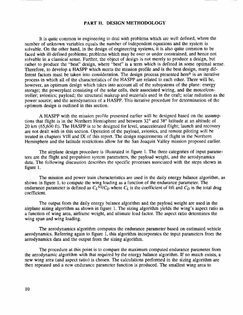
PART II. DESIGN METHODOLOGY
It is quite common in engineering to deal with problems which are well defined, where thenumber of unknown variables equals the number of independent equations and the system is
solvable. On the other hand, in the design of engineering systems, it is also quite common to be
faced with ill-defined problems; problems which may be over or under constrained, and hence not
solvable in a classical sense. Further, the object of design is not merely to produce a design, but
rather to produce the "best" design, where "best" is a term which is defined in some optimal sense.
Therefore, to develop a HASPP which meets the mission profile and is the best design, many dif-
ferent factors must be taken into consideration. The design process presented here 6 is an iterative
process in which all of the characteristics of the HASPP are related to each other. There will be,
however, an optimum design which takes into account all of the subsystems of the plane: energy
storage; the powerplant consisting of the solar cells, their associated wiring, and the motor/con-
troller; avionics; payload; the structural makeup and materials used in the craft; solar radiation as the
power source; and the aerodynamics of a HASPP. This iterative procedure for determination of the
optimum design is outlined in this section.
A HASPP with the mission profile presented earlier will be designed based on the assump-
tions that flight is in the Northern Hemisphere and between 32 ° and 38 ° latitude at an altitude of
20 km (65,600 ft). The HASPP is to be designed for level, unaccelerated flight; launch and recoveryare not dealt with in this section. Operation of the payload, avionics, and remote piloting will be
treated in chapters VIII and IX of this report. The design requirements of flight in the Northern
Hemisphere and the latitude restrictions allow for the San Joaquin Valley mission proposed earlier.
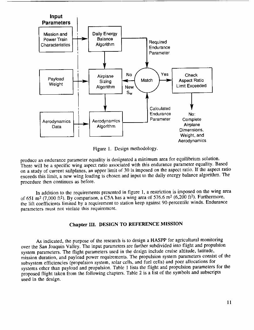
The airplane design procedure is illustrated in figure 1. The three categories of input parame-
ters are the flight and propulsion system parameters, the payload weight, and the aerodynamics
data. The following discussion describes the specific processes associated with the steps shown in
figure 1.
The mission and power train characteristics are used in the daily energy balance algorithm, as
shown in figure 1, to compute the wing loading as a function of the endurance parameter. Theendurance parameter is defined as CL3/2/Co where Ca is the coefficient of lift and CD is the total dragcoefficient.
The output from the daily energy balance algorithm and the payload weight are used in the
airplane sizing algorithm as shown in figure 1. The sizing algorithm yields the wing's aspect ratio as
a function of wing area, airframe weight, and ultimate load factor. The aspect ratio determines the
wing span and wing loading.
The aerodynamics algorithm computes the endurance parameter based on estimated vehicle
aerodynamics. Referring again to figure 1, this algorithm incorporates the input parameters from the
aerodynamics data and the output from the sizing algorithm.
The procedure at this point is to compare the maximum computed endurance parameter from
the aerodynamic algorithm with that required by the energy balance algorithm. If no match exists, a
new wing area (and aspect ratio) is chosen. The calculations performed in the sizing algorithm are
then repeated and a new endurance parameter function is produced. The smallest wing area to
10
InputParameters
Mission and t
Power TrainCharacteristics
PayloadWeight
AerodynamicsData
Daily EnergyBalance
Algorithm
AirplaneSizing
Algorithm
AerodynamicsAlgorithm
RequiredEnduranceParameter
f
L.oS es
I CalculatedI EnduranceI Parameter
Figure 1. Design methodology.
Check
Aspect RatioLimit Exceeded
No:
CompleteAirplane
Dimensions,
Weight, andAerodynamics
produce an endurance parameter equality is designated a minimum area for equilibrium solution.There will be a specific wing aspect ratio associated with this endurance parameter equality. Based
on a study of current sailplanes, an upper limit of 30 is imposed on the aspect ratio. If the aspect ratio
exceeds this limit, a new wing loading is chosen and input to the daily energy balance algorithm. The
procedure then continues as before.
In addition to the requirements presented in figure 1, a restriction is imposed on the wing area
of 651 m 2 (7,000 ft2). By comparison, a C5A has a wing area of 576.6 m 2 (6,200 ft2). Furthermore,
the lift coefficients limited by a requirement to station keep against 90-percentile winds. Enduranceparameters must not violate this requirement.
Chapter III. DESIGN TO REFERENCE MISSION
As indicated, the purpose of the research is to design a HASPP for agricultural monitoring
over the San Joaquin Valley. The input parameters are further subdivided into flight and propulsion
system parameters. The flight parameters used in the design include cruise altitude, latitude,
mission duration, and payload power requirements. The propulsion system parameters consist of the
subsystem efficiencies (propulsion system, solar cells, and fuel cells) and poer allocations for
systems other than payload and propulsion. Table 1 lists the flight and propulsion parameters for the
proposed flight taken from the following chapters. Table 2 is a list of the symbols and subscripts
used in the design.
11
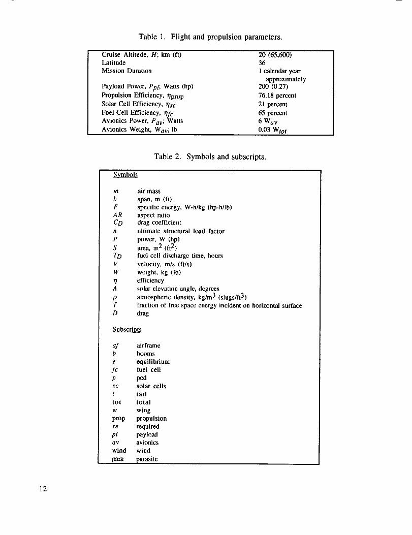
Table 1. Flight and propulsion parameters.
Cruise Altitude, H; km (ft)Latitude
Mission Duration
Payload Power, Ppl; Watts (hp)
Propulsion Efficiency, r/propSolar Cell Efficiency, r/sc
Fuel Cell Efficiency, r/fcAvionics Power, Pav; Watts
Avionics Weight, Wav; lb
20 (65,600)
36
1 calendar year
approximately200 (0.27)
76.18 percent
21 percent
65 percent
6 Way
0.03 Wto t
Table 2. Symbols and subscripts.
mb
FAR
coelP
S
TDV
W
77A
PT
D
air mass
span, m (ft)
specific energy, W-h/kg (hp-h/lb)aspect ratiodrag coefficient
ultimate structural load factor
power, W (hp)
area, m 2 (ft 2)
fuel cell discharge time, hours
velocity, m/s (ft/s)
weight, kg (lb)
efficiency
solar elevation angle, degrees
atmospheric density, kg/m 3 (slugs/ft 3)
fraction of free space energy incident on horizontal surface
drag
Subscripts
af airframeb booms
e equilibrium
fc fuel cell
p podsc solar cells
t tail
tot total
w wing
prop propulsion
re required
pl payloadav avionics
wind wind
para parasite
12

The goal of the design methodology is to compare all of the parameters and determine if
stable flight is feasible under the prescribed conditions. The airplane is defined to be in equilibrium
when there is an energy balance between the available solar power per unit area and the required
total power per unit wing planform area. When the airplane is in equilibrium, it is said that it crui_s
at an equilibrium altitude. Equilibrium conditions are shown by the sketch in figure 2, describing the
daily energy balance algorithm. Figure 2 illustrates the power produced and the total power
consumption for any particular day.
December 2213
12
11
10
8
6_ 5
a
2
1
0 o
Solar Cell Power ..... /" ''_/ ;
- 65-Percent Power ,/ ',
Propulsion Power /
Avionics Power / ;
- Payload Power /- ' I _,,._N,,, ;
- s_ ,,o, ir/'77777"7"?777777772T ..... "-7")'7777777177771"7"7I
4 8 12 16 20 24Time (hours)
Figure 2. Daily energy balance algorithm.
The total power required for flight is:
Ptot = Pprop+Pav+Ppl (1)
The avionics power, Pay, is the power component required for maneuvering flight and vehicle control.
The payload power, Ppt, is the power component required by the payload and all of its functions. Forthe mission proposed here, the payload will be the agricultural sensors, and the payload power
requirements will include data handling and transmission.
The power produced by the solar cells, Psc, is a function of the solar constant, the atmospheric
transmittance, the efficiency of the solar cells, and the solar elevation angle. It is given by:
Psc/S = 1,353 T qsc sin A (W/m 2) . (2)
The atmospheric transmittance or the fraction of free-space radiation is discussed in chapter IV. Thesolar constant, 1,353 W/m 2 (125.8 W/ft2), is the amount of solar radiation available at the edge of
the atmosphere computed for all wavelengths. Equation (2) may be evaluated to produce Psc/S as a
function of time as shown in figure 2. In figure 2. the total power area B must be provided by the fuel
cell to maintain equilibrium flight, while area A represents the total power per unit area produced by
13

thesolarcells abovewhat is requiredto maintainflight. This solutionaccountsfor both storedenergyanddirect energy from the solar cells being used during brief periods at sunrise and sunset.Equilibrium conditions exist when:
(area A) (r/yc) = the sum of (area B) (3)
Minimum design specifications require that the energy balance calculation be performed for the day ofleast available solar radiation, December 22.
The power required to maintain cruise flight is defined as :
Pprop/Sw = (2//9) 1/2 (Wtot/Sw) 312 (CD/CL 3/2) (1.356/r/prop) ,
where the constant 1.356 converts ft-lb/s to Watts using an English system of units. In typical
airplane design, the power required is given as a function of the velocity of the vehicle and its totaldrag. Equation (4) is derived in the following manner:
Assuming:
Lift = Weight/cos (a)
(where cos (a), the angle of incidence, is -= 1)
Lift = (/9/2) (V 2) (Sw) (CL)
Drag = (p/2) (V 2) (Sw) (Co)
Pre = (V) (D) .
Combining equations (5a) and (5b) yields:
V = [(2 W)/(p Sw CD] la ,
and substituting equation (5c)into (5d) yields:
Pre = (p/2) (V3)S,,) (Co) •
Now, combining equations (5e) and (50 results in:
Pre = (/9/2) [2(W)/R(Sw) (CL)] 3/2 (Sw) (Co)
or
(4)
(5a)
(5b)
(5c)
(5d)
(5e)
(50
Pre = [2]/911/2 W3/2 [1/Sw 1/2] Co/CL 3a ,
which is equation (4) when divided by S_ and multiplied by the propulsion system efficiency factor.
Equations (1) and (4) can be combined to give the total power required per unit wing area as:
14
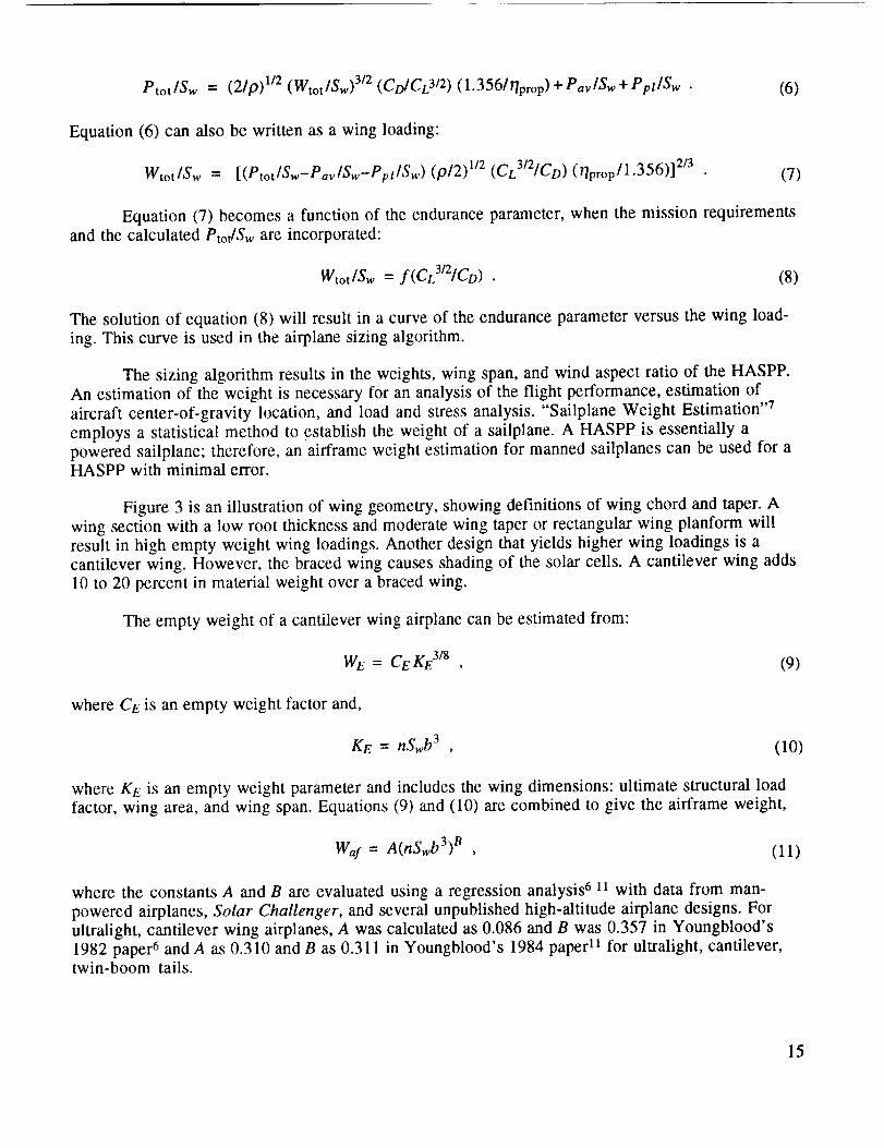
Ptot/Sw = (2/P) 1/2 (Wtot/Sw) 3/2 (CD]CL 3/2) (1.356/r/prop) +Pav ]Sw + Ppl/Sw • (6)
Equation (6) can also be written as a wing loading:
Wtot/Sw = [(Ptot/Sw-Pav/Sw-Ppl/Sw) (P/2) 1/2 (CL3/2]CD) (r/prop/1.356)] 2/3 (7)
Equation (7) becomes a function of the endurance parameter, when the mission requirements
and the calculated Ptot/Sw are incorporated:
Wtot [Sw = f(CL3/2/CD) • (8)
The solution of equation (8) will result in a curve of the endurance parameter versus the wing load-
ing. This curve is used in the airplane sizing algorithm.
The sizing algorithm results in the weights, wing span, and wind aspect ratio of the HASPP.
An estimation of the weight is necessary for an analysis of the flight performance, estimation of
aircraft center-of-gravity location, and load and stress analysis. "Sailplane Weight Estimation ''7
employs a statistical method to establish the weight of a sailplane. A HASPP is essentially a
powered sailplane; therefore, an airframe weight estimation for manned sailplanes can be used for aHASPP with minimal error.
Figure 3 is an illustration of wing geometry, showing definitions of wing chord and taper. A
wing section with a low root thickness and moderate wing taper or rectangular wing planform will
result in high empty weight wing loadings. Another design that yields higher wing loadings is a
cantilever wing. However, the braced wing causes shading of the solar cells. A cantilever wing adds
10 to 20 percent in material weight over a braced wing.
The empty weight of a cantilever wing airplane can be estimated from:
WE = CE KE 318 , (9)
where CE is an empty weight factor and,
KE = nSwb 3 , (10)
where KE is an empty weight parameter and includes the wing dimensions: ultimate structural load
factor, wing area, and wing span. Equations (9) and (10) are combined to give the airframe weight,
Waf = A(nSwb3) B (11)
where the constants A and B are evaluated using a regression analysis 6 11 with data from man-
powered airplanes, Solar Challenger, and several unpublished high-altitude airplane designs. For
ultralight, cantilever wing airplanes, A was calculated as 0.086 and B was 0.357 in Youngblood's
1982 paper 6 and A as 0.310 and B as 0.311 in Youngblood's 1984 paper ll for ultralight, cantilever,twin-boom tails.
15

An understandingof wing geometryis neededto completethe sizingalgorithm. Referringagainto figure 3, the distancefrom onewing tip to anotheris the wing span,b. The chord, c, is the
distance from the leading edge to the trailing edge measured parallel to the plane of symmetry in
which the centerline chord, Co, lies. The chord will vary along the length of the wing, so a mean chord,c,,,, is used. The wing planform area is expressed as:
Sw = crab . (12)
The aspect ratio, AR, is a ratio of the square of the wing span to wing area or,
AR = b21Sw = blc = Sw/c 2 (13)
For sailplanes, 7 the wing chord typically changes with the span to maintain a constant wing area.
The aspect ratio is usually proportional to the square of the span for spans up to 15 m (49.2 ft). For
spans greater than 15 m, the aspect ratio tends to be proportional to the first power of the span.Figure 3 also illustrates a wing taper or taper ratio, A., the ratio of the tip chord, ct, to the midspanchord, Co. It is:
,71.= ct/Co . (14)
For sailplanes with wings that are not straight tapered, a taper ratio of root chord, Cr, to mean chord
has proven to be more practical.
I V (of air relative to wind)
I i 1-I It ' !I
q
Midspan Chord c oTip Chord c tWing Span b
Chord @ y cMean Chord s/b
Aspect Ratio b2/SPlanform Area S
Figure 3. Top view of a wing (planform).
16
Theairframe weight cannow bederivedfrom equation(11)as:
Waf = 0.310 (nSwb3) 0"311 , (15)
or, with equation (13) as:
War = 0.310 [nSw(AR Sw)3/2] 0"311 (16)
Equation (16) yields the airframe weight loading:
WarlSw = 0.310 [n 0.311 AR 0'467 Sw -0'222] . (17)
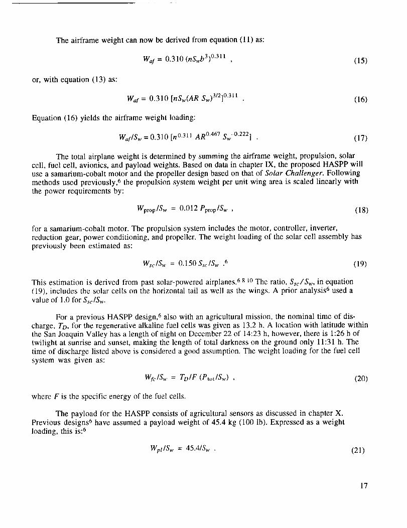
The total airplane weight is determined by summing the airframe weight, propulsion, solar
cell, fuel cell, avionics, and payload weights. Based on data in chapter IX, the proposed HASPP willuse a samarium-cobalt motor and the propeller design based on that of Solar Challenger. Following
methods used previously, 6 the propulsion system weight per unit wing area is scaled linearly with
the power requirements by:
WproplSw = 0.012 eprop/Sw , (18)
for a samarium-cobalt motor. The propulsion system includes the motor, controller, inverter,
reduction gear, power conditioning, and propeller. The weight loading of the solar cell assembly has
previously been estimated as:
Wsc/Sw = 0.150 Ssc/Sw .6 (19)
This estimation is derived from past solar-powered airplanes. 6 8 lo The ratio, Ssc/Sw, in equation
(19), includes the solar cells on the horizontal tail as well as the wings. A prior analysis 6 used a
value of 1.0 for Ssc/Sw.
For a previous HASPP design, 6 also with an agricultural mission, the nominal time of dis-charge, To, for the regenerative alkaline fuel cells was given as 13.2 h. A location with latitude within
the San Joaquin Valley has a length of night on December 22 of 14:23 h, however, there is 1:26 h of
twilight at sunrise and sunset, making the length of total darkness on the ground only 11:31 h. The
time of discharge listed above is considered a good assumption. The weight loading for the fuel cell
system was given as:
Wfc/Sw = TD/F (Ptot/Sw) , (20)
where F is the specific energy of the fuel cells.
The payload for the HASPP consists of agricultural sensors as discussed in chapter X.
Previous designs 6 have assumed a payload weight of 45.4 kg (100 lb). Expressed as a weight
loading, this is: 6
Wpl/S w : 45.4/Sw . (21)
17

The HASPPavionicsweight loading,Wav/Sw, is given by approximations presented in chapter XI.
The airframe wing loading can be expressed as:
Waf/Sw = Wtot/Sw-Wprop/Sw-WsclSw-Wfc/Sw-Wpl/Sw-Wav/Sw, (22)
where the components of this equation can be seen in equations (18) through (21). This airframeweight loading was also seen in equation (17), which can be written in terms of the aspect ratio as:
AR = [(Waf/Sw) Sw°222/(0.310 nO.311)] 2"141 (23)
Substituting equation (22) into equation (24) yields the aspect ratio in terms of airframe weight
loading, wing area, and ultimate load factor.
The load factor is the ratio of the load supported by the wings to the actual weight of the
aircraft and its contents. The load factor is expressed in "G" units or multiples of the local gravi-tational constant measured at the Earth's surface. The load on the wings of an aircraft increases in a
bank and with aircraft speed. For example, an aircraft in level turning flight with a 60 ° bank under-
goes a centripetal acceleration of 2 G's. Wind gusts will increase the load factor, more so at higher
aircraft speeds. The limit load factor is the load factor that an aircraft can sustain without incurring
permanent structural damage, while the ultimate load factor is twice the limit load factor. Airplanes
certified by the Federal Aviation Administration (FAA) in the normal category are required to have
a minimum limit load factor of 3.8, for a 75 ° bank. Typically, 7 the ultimate load factor for sailplanes is8, however, since the HASPP is unmanned and will fly slowly at altitudes above most turbulence, anultimate load factor of 4 is used here.
The calculations presented in the sizing algorithm are sufficient to determine the dimensionsand weights of the HASPP, which are necessary for the aerodynamics algorithm as shown in
figure 1.
An endurance parameter based on vehicle aerodynamics must be derived with this algorithm.This endurance parameter should equal or exceed that calculated by the energy balance algorithm.
The aerodynamics of the surfaces of the HASPP must be studied in order to calculate the endurance
parameter. Due to the low speed of a HASPP, the airfoils will operate in a Reynolds number range of105 to 10 6 .
Typically, the horizontal and vertical tail surfaces operate at low values of CL. As a result, the
induced drag of these surfaces is small. The NACA 0008-34 airfoil has been used in previous
designs 6 for the tail, providing thin, low drag surfaces. The zero-lift tail drag coefficient for this airfoilis: 6
(Coo)t = 0.0075 StlSw , (24)
where St is the area of both the vertical and horizontal tail surfaces. Since the horizontal tail is
oversized to allow for mounting of solar cells on the stabilizer, St/Sw was assumed to be 0.36. This
value will be used in this design.
18

The fuel cells, avionics,andpayloadwill becarriedin a low-dragpod beneaththecentersectionof the wing. A previousdesignassumedthepod to havea length-to-diameterratio of 3 to1. 6 For a Reynolds number of 10 6, this pod has a drag coefficient of 0.06. 6 This gives a zero-lift drag
coefficient for the pod of: 6
(Coo)p = 0.06 Sp/Sw. (25)
For a past solar HAPP design, 6 a twin boom tail configuration was used with an estimated dragcoefficient of:
(COo)b = 0.0003 . (26)
The drag buildup method allows the component zero-lift drag coefficients to be added
together to give the total airplane drag coefficient. The resultant equation is:
Co = (CDo)w+(CDo)t+(CDo)p+(CDo)b+[( 1 + tS)l(zc *AR)]C 2 (27)
The last term in equation (27) is the wing-induced drag where t_ is a constant equal to 0.11 for an
outer wing panel taper ratio of 0.5. The (1+6) term also refers to an airplane efficiency factor of 90
percent.
With the definition of the endurance parameter and the drag coefficient given by equation
(27), the endurance parameter reduces to a function of a single variable, the lift coefficient. This
endurance parameter is compared with that obtained from the energy balance algorithm, equation (8)
as shown in figure 1. This procedure is repeated until an endurance parameter equality is achieved at
the smallest wing area possible. Equilibrium flight will be possible only at the lift coefficient asso-
ciated with this endurance parameter. 6 The additional limitations on aspect ratio and wing area,
mentioned earlier, must also be maintained for equilibrium flight to exist.
The lift coefficient must enable the HASPP to stay on course against 90-percentile winds.
This requirement is: 6
CL <= (CL)wind = 2 (Wtot]Sw)](p Vwin 2) . (28)
When this design procedure is completed with all of the requirements satisfied, the
specifications of a feasible HASPP for the given mission will be determined.
Chapter IV. SOLAR RADIATION
A study of solar radiation is instrumental in the calculation of power available to the airplane.The radiation available varies as a function of time throughout the mission as well as a number of
other parameters which are determined by the mission profile. Thus, the power available to maintain
flight and operate equipment is continually changing. The maximum available radiation changes from
minute to minute due to the rotation of the Earth. Further, there is a day-to-day change due to the
change of the inclination of the Earth's rotational axis. Optimum aircraft design specifications must
be based on minimum solar radiation availability.
19
At theoperatingaltitudeof 20km (65,600ft), a HASPPwill beaboveall cloud coverso therewill beno daytimeinterruptionof sunlight.The solarradiation,incidenton thesolar cells of theairplane,is a function of theair massandthe solar-altitudeangle.The air massis definedas thepathlength of sunlight,or thequantity of atmospherethat solarradiationcanpassthrough, andisequal to the cosecantof thesolar altitudeangle,A. Air mass is also a function of altitude and is
represented by m(z,A) where sea level is given by z = 0. The solar-altitude angle is the anglebetween the incident solar rays and the horizontal. It is a function of the declination of the Sun, the
time of year, the time of day, and the latitude.
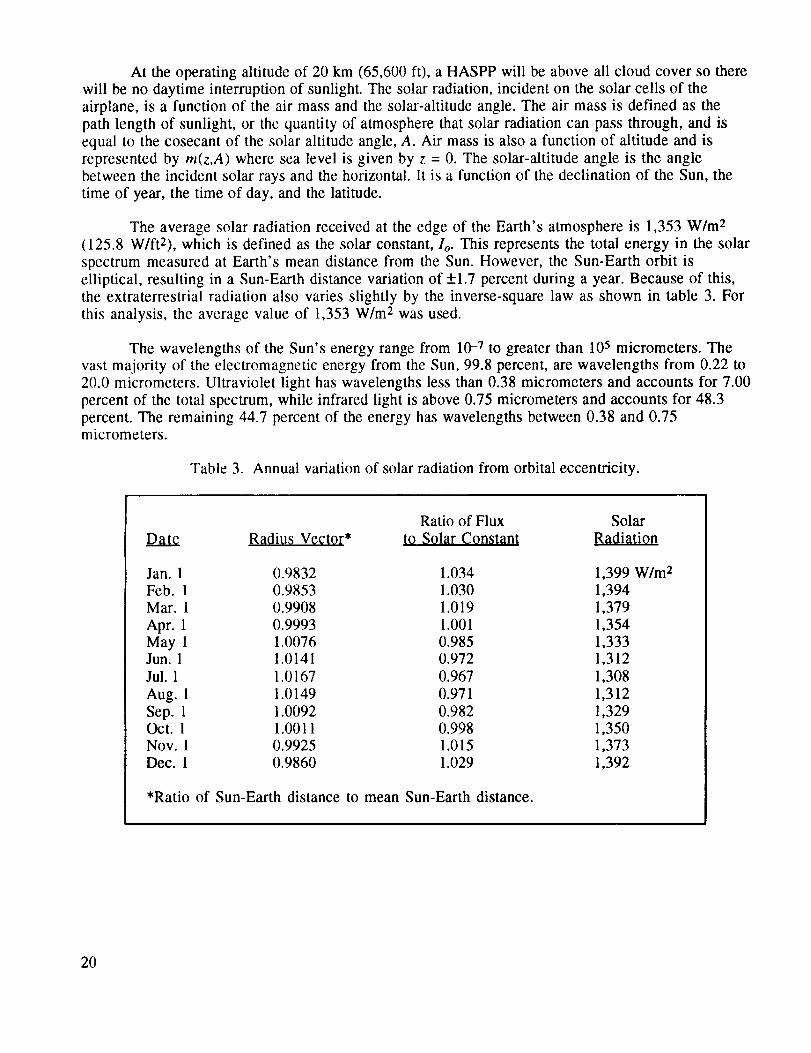
The average solar radiation received at the edge of the Earth's atmosphere is 1,353 W/m 2
(1125.8 W/ft2), which is defined as the solar constant, Io. This represents the total energy in the solar
spectrum measured at Earth's mean distance from the Sun. However, the Sun-Earth orbit is
elliptical, resulting in a Sun-Earth distance variation of +1.7 percent during a year. Because of this,
the extraterrestrial radiation also varies slightly by the inverse-square law as shown in table 3. For
this analysis, the average value of 1,353 W/m 2 was used.
The wavelengths of the Sun's energy range from 10 -7 tO greater than 105 micrometers. The
vast maiority of the electromagnetic energy from the Sun, 99.8 percent, are wavelengths from 0.22 to
20.0 micrometers. Ultraviolet light has wavelengths less than 0.38 micrometers and accounts for 7.00
percent of the total spectrum, while infrared light is above 0.75 micrometers and accounts for 48.3
percent. The remaining 44.7 percent of the energy has wavelengths between 0.38 and 0.75micrometers.
Table 3. Annual variation of solar radiation from orbital eccentricity.
Ratio of Flux Solar
Date Radius Vector* to Solar Constant Radiation
Jan. 1 0.9832 1.034
Feb. 1 0.9853 1.030
Mar. 1 0.9908 1.019
Apr. 1 0.9993 1.001
May 1 1.0076 0.985Jun. 1 1.0141 0.972
Jul. 1 1.0167 0.967
Aug. 1 1.0149 0.971
Sep. 1 1.0092 0.982Oct. 1 1.0011 0.998Nov. 1 0.9925 1.015
Dec. 1 0.9860 1.029
*Ratio of Sun-Earth distance to mean Sun-Earth distance.
1,399 W/m 2
1,394
1,3791 354
1 333
1 312
1 308
1 312
1 329
1 350
1 373
1,392
20

Bouger's law is usedin calculatingtheatmosphericabsorptionof solar radiationfor clearskies. It is:
/b =Io_ km , (29)
where Ib and Io are the terrestrial and extraterrestrial intensities of beam radiation, respectively, k
is an absorption constant for the atmosphere, and m is the air mass as shown in figure 4.
Atmospheric7 _ C
Lay.__ ,_
[-_ Alpha
Sun
Alpha = Solar Altitude Angle Angle
Air Mass = Path Length of Sunlight= BP/CP -- csc ALPHA = M
M = 0, Extraterrestrial Radiation
M = 1, Sun is Directly Overhead
Atmosphere is Idealized as a Constant Thickness Layer.
Figure 4. Air mass definition.
The solar-altitude angle, A, can be calculated using the law of cosines for spherical triangles.The result is:
sin A = cos D cos H cos L + sin L sin D , (30)
where D is the declination of the Sun between +23.5 ° and -23.5% D = [23.5 sin (360 d/365)] °, or the
angle between the Sun's rays and the zenith direction (directly overhead) at noon on the Earth's
Equator; d is the time of year in days from the vernal equinox; L is the latitude; and H is the solar
hour angle. The solar hour angle is defined as H = (t/24)360 ° = 15t °, where t is the time from solarnoon or local solar time in hours.
Atmospheric transmittance, Tat m - (Ibllo), is a ratio of extraterrestrial solar radiation and
solar radiation that has passed through the atmosphere, and it is given by:
Tatm = 0.5( e -0.65m(z'A ) + e-O'O95m(z'A )) , (31)
where m(z,A) is the air mass at an altitude z above sea level given by:
m(z,A ) = rn(O,A )[p(z)lp(O)] , (32)
where p(z) is the atmospheric pressure at altitude z. The sea level air mass is:
21

m(0,A) = [1,229+(614 sin A)2]°5-614 sin A .
Therefore, the surface beam radiation, lb, for the clear sky conditions is:
Ib = loTatm •
(33)
(34)
Equations (31) and (33) represent an accuracy improvement over equation (29) since they include
curvature effects. Equation (31) can be modified to account for particulates and water vapor in the air
by:
Tatm = ao+ale-k csc A , (35)
where ao, ab and k are only functions of altitude and visibility as shown in table 4. The coefficients inthe table were calculated for the 1962 Standard Atmosphere. The operating altitude of the airplane in
this design renders the use of equation (35) unimportant.
Table 4. Coefficients ao, al, and k calculated for the 1962 Standard Atmosphere for use in
determining solar transmittance t.
Altitude above sea level (km)
0 0.5 1 1.5 2 (2.5)
23 km haze model
ao 0.1283 0.1742 0.2195 0.2582 0.2195 (0.320)
al 0.7559 0.7214 0.6848 0.6532 0.6265 (0.602)k 0.3878 0.3436 0.3139 0.2910 0.2745 (0.268)
5 km haze model
ao 0.0270 (0.063) 0.0964 (0.126) (0.153) (0.177)
al 0.8101 (0.804) 0.7978 (0.793) (0.788) (0.784)
k 0.7552 (0.573) 0.4313 (0.330) (0.269) (0.249)
a. Adapted from Hottel by permission.b. Values in parentheses indicate interpolated or extrapolated values.
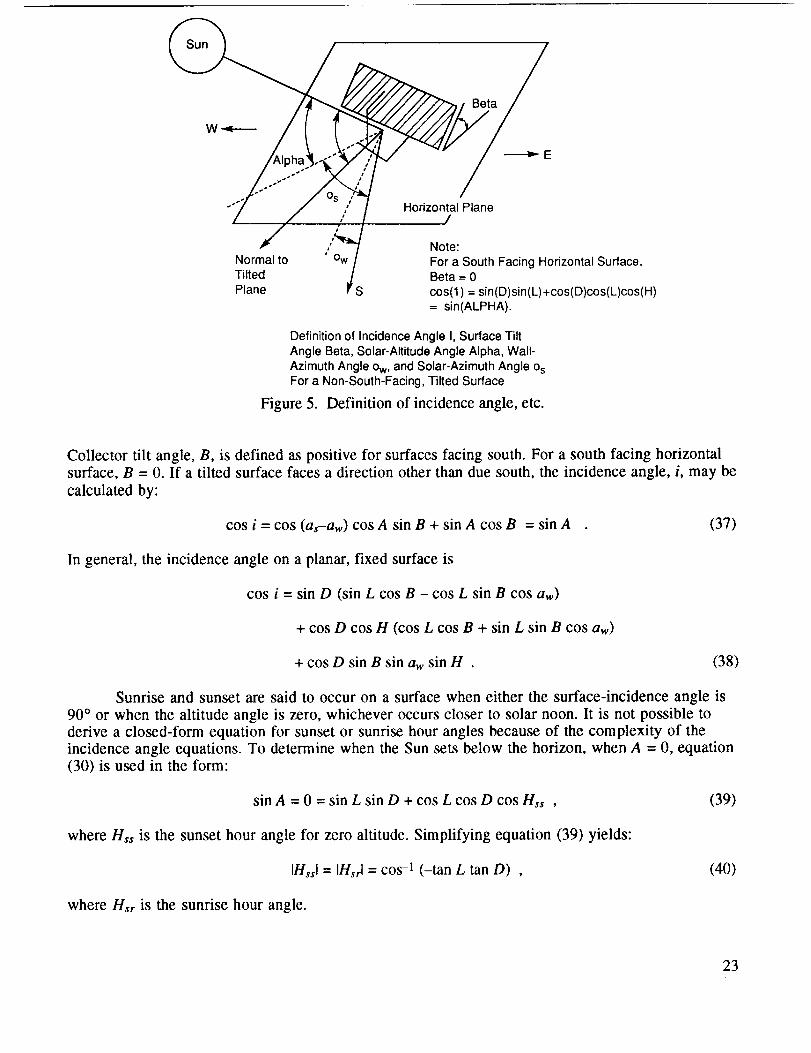
Assuming for discussion purposes that the HASPP is a fixed surface in the atmosphere, the
incidence angle is dependent on the basic solar angles, D, H, and L, and on the two angles that
characterize the surface orientation, B and aw. The wall-azimuth angle, aw, is defined in the same
manner as the solar azimuth angle and is shown in figure 5. The solar-azimuth angle can be com-
puted from:
sin as = (cos D sin H)/cos A. (36)
22
Horizontal Plane/
Note:
For a South Facing Horizontal Surface,Beta = 0
cos(l) = sin(D)sin(L)+cos(D)cos(L)cos(H)= sin(ALPHA).
Definition of Incidence Angle I, Surface TiltAngle Beta, Solar-Altitude Angle Alpha, Wall-Azimuth Angle ow, and Solar-Azimuth Angle osFor a Non-South-Facing, Tilted Surface
Figure 5. Definition of incidence angle, etc.
Collector tilt angle, B, is defined as positive for surfaces facing south. For a south facing horizontalsurface, B = 0. If a tilted surface faces a direction other than due south, the incidence angle, i, may be
calculated by:
cos i = cos (as--aw) cos A sin B + sin A cos B = sin A (37)
In general, the incidence angle on a planar, fixed surface is
cos i = sin D (sin L cos B - cos L sin B cos aw)
+ cos D cos H (cos L cos B + sin L sin B cos aw)
+ cos D sin B sin aw sin H . (38)
Sunrise and sunset are said to occur on a surface when either the surface-incidence angle is
90 ° or when the altitude angle is zero, whichever occurs closer to solar noon. It is not possible toderive a closed-form equation for sunset or sunrise hour angles because of the complexity of the
incidence angle equations. To determine when the Sun sets below the horizon, when A = 0, equation
(30) is used in the form:
sin A = 0 = sin L sin D + cos L cos D cos Hss , (39)
where H,s is the sunset hour angle for zero altitude. Simplifying equation (39) yields:
Inssl = Insrl = cos -1 (-tan L tan D) , (40)
where Hsr is the sunrise hour angle.
23

Total beam radiation for given periods of time on a surface is given by:
to
/tot I Ib(t) cos i(t)dt
to+(St) (41)
where (&) is the tine interval. The function Ib(t) depends on local weather and microclimate.
Further, the form of Ib(t) is generally not known. Therefore, equation (41) is not useful. However, it
is possible to calculate /tot outside the Earth's atmosphere since Ib(t) is the solar constant multi-plied by the orbital eccentricity factor e(t). This is similar to equation (29) and is
lb(t) = e(t) Io . (42)
The orbital eccentricity factor, e(t), may be taken from table 3 or:
e(t) -- 1+0.034 cos [2zrn(t)/365] , (43)
where n is the number of days from January 1. Combining equations (41) and (42) yields:
to
/tot I loe(t) sin A(t)dt
,o+_S,) (44)
Thus, equations (30) and (43) combine to give a daily total:
0
/day = 24Dr I Io[ 1 +0.034 cos (2zrn/365)] sin Adt
Hsr (45)
where Hsr must be in units of radians.
Chapter V. SOLAR CELLS
The choice of solar cells is one of the most important decisions in the design of a HASPP.
There are single crystal cells, concentrator cells, tandem and thin film cells, and a variety of cell
materials in each of these categories. The chosen cell must have the best combination of efficiency,
durability under the mission conditions, bandgap, weight, and life expectancy.
The French physicist, Edmund Becquerel, initially observed the photovoltaic effect in a weak
conducting solution in 1839. However, the first solar cell was not produced until 1954 when BellLaboratory produced a silicon cell with an efficiency of 4 percent. Since then, efficiencies have
improved significantly with a number of different semiconductor materials being used to make solar
cells. The most common materials are gallium arsenide, cadmium telluride, copper indium diselenide,
and crystalline and amorphous silicon. Each of these materials have properties that make themdesirable for a particular purpose.
All solar cells have a common configuration, with two or more layers of semiconductor
material. The atoms of the semiconducting layers absorb photons of light which free electrons
24

producingholesto conductcurrent.The interface of the two different semiconductor materials in the
cell creates a voltage potential that propels electrons through a circuit. Some of the limiting factors
common to all cells are: the quality of material, shading of the cell by the grid, carrier recombination,
light absorption, reflection of light from the cell surface, series and contact resistances, and the frac-tion of wavelengths of available light that can be absorbed. There are also losses common to mostcells that include: band-to-band Auger recombination, emitter recombination, and resistive voltage
drops. Many advances have recently been made in photovoltaic cells including transparent conduct-
ing oxides, flexible substrates, laserscribed connections, microgrooved surfaces, point contacts,
multijunctions, and light-capturing techniques. In addition, improvements such as internal reflection,backsurface reflectors, and antireflection coatings have been made to allow the cells to collect and
hold the maximum radiation possible.
A. Solar Array Configuration
Solar cells on a HASPP must be made into an array and placed on or in the wings and hori-
zontal tail. In an array, the cells in series should be matched for current and the cells in parallel
should be matched for voltage. Typically, the performance of an array is diminished as the area is
increased. However, this may not be true of the gallium arsenide thin films. The 5- to 10-percent
power loss found in most thin film modules can be attributed to interconnect area loss and seriesresistance losses. This is indicative of early stage thin film development and should improve with
further research. 3° Thirty to fifty cells may be wired together in series to form a module of 0.09 to
0.37 m 2 (1 to 4 ft 2) of area. An arm is composed of several modules and an array is made from
several arms. Modules are typically wired in parallel to permit the current to bypass a broken or
shaded cell without overloading adjacent cells or shutting off the current from the remaining good
cells in that series. Solar Challenger used 144×3 cell strings connected through a diode to a panel
bus, permitting testing of individual strings. Each panel was protected by a 10-A fuse. The power
supply was split into five parts to limit the inrush current.
B. Solar Cell Characteristics
Solar cells are characterized by their efficiency, bandgap, and performance features. Each of
these factors is determined by the semiconductor material and the device configuration chosen. The
solar array efficiency is used in the calculation of power per unit area produced. This in turn is used
as input to the energy balance algorithm, which determines the feasibility of the aircraft. The effi-ciency of photovoltaic devices is dependent on several parameters. Solar cell efficiency is defined as
the ratio of the electrical energy output from a cell to the sunlight energy incident on the cell. The
current from a cell increases linearly (approximately) with increasing sunlight intensity. The voltage
produced by a cell is approximately proportional to the log of the intensity. Increased current densityresults in increased resistive losses.
The air mass at which a cell operates is also a factor which affects cell efficiency. A cell will
produce more power at higher altitudes and in space than at the surface of the Earth; there are fewer
atmospheric particles to block the sunlight. However, the efficiency of the cell is actually lower due to
the wider range of wavelengths of light incident on the cell. The semiconductor material in a solar cellhas a relatively limited bandgap, or threshold energy at which solar photons are usable. The bandgap
is expressed as a range of frequencies or wavelengths to which cells are sensitive. A photovoltaicmaterial will absorb light whose energy is greater than their bandgap. Light with less energy passes
through the cell. Essentially, at the surface of the Earth, the solar energy available is concentrated in
a comparatively narrow frequency band. For most cells the bandgap of the semiconductor falls within
25

the bandof the availablesolarenergyat thesurfaceof theEarth.As the elevationof the cellincreases,the energyavailable increasesinsideandoutsidethe bandgapof the cell. The result isthat while moretotal energy is available,theamountof theenergyoutsidethebandgapof thecellincreasesfaster,thusthe efficiency of the cell decreaseswith altitude.
It hasbeenestimatedthat theefficiency of a silicon cell at AM0 (air mass0 or spacecondi-tions)will be2 to 3 percentof that at AM1.5, (whentheincidenceangleof the Sun'srays is 45°).Theefficiency of acopperindium diselenide(CIS) cell at AM0 hasbeen evaluated to be 90 percent of
the AM1.5 efficiency.
The ambient temperature at which a cell operates affects the efficiency of the cell. As the
temperature decreases, the voltage available increases and the current produced decreases. As an
example, the efficiency of a CIS cell will increa_ from 12.4 percent at 25 °C (77 °F) to 19.4 percentat-107 °C (-161 °F).
C. Semiconductors
The most commonly used semiconductor materials are either crystalline or polycrystatline.Gallium arsenide and silicon are used to make single-crystal cells, while amorphous silicon,
cadmium telluride, and copper indium diselenide are used to make thin film photovoltaic devices.
Gallium arsenide is unique in that it can be used to make single-crystal thin films. Companies that
manufacture these photovoltaic devices measure their efficiencies using a solar simulator rather than
the solar spectrum. They all publish their results as measured at 25 °C (77 °F) and AM1.5.
1. Gallium Arsenide
The photovoltaic device with the highest efficiency, to date, is the gallium arsenide, Ga-As,single-crystal cell. Ga-As has a bandgap of 1.43 eV at room temperature and the bandgap goes up
as the temperature decreases. The efficiency of a 0.5- by 0.5- by 0.051-cm (0.2- by 0.2- by 0.02-in)
cell has been recorded at 24 percent. A thin-film, single-crystal Ga-As cell that measures 1 cm 2
(0.16 in 2) by 5 to 6 micrometers (1.97 to 2.36 by 10 -4 in) thick is as flexible as any other thin film
device, but since it is a crystal it has a much higher efficiency than polycrystalline semiconductors. A2-cm 2 (0.31-in 2) Ga-As cell can be manufactured which is over 22-percent efficient. Cells can be
made which are as large as 16 cm 2 (2.48 in2).
KOPIN Corporation manufactures Ga-As cells and claims that their modules are as efficient
as the individual cells since they suffer no fill factor losses. Placed on a 51- to 76-micrometer (2- to
3-mil) thick glass substrate, the cell can flex according to the limitations of the glass. It is estimated
that a 2-mil thick glass substrate would have a radius of curvature of 2 in. Normally, a cell needs a
cover glass to protect the cell and the adhesive. An alternative to using a cover glass is encapsula-
tion of the cell. This process is also called direct glassing and would eliminate the problem of the
inflexibility of the cover glass.
Although the cells have not previously been mounted to a plastic, KOPIN believes therewould be no problem in mounting the thin films to Mylar. Furthermore, Ronald Gale of KOPIN states
that their cells are certified for space use so the thermal cycling of cells at altitude should not be a
problem. KOPIN has measured a single-crystal thin film Ga-As cell at 22.4-percent efficiency at
26
AM1.5. At AM0, theefficiency wouldbeabout21percent.Thecell would consistof a 2- to 4-milthick glasssubstrate,1to 2 mils of adhesive,q4 mil of Ga-As, and 1 to 2 mils of encapsulation
dependent on the radiation present.
Ga-As does not degrade with exposure to sunlight and is more radiation resistant than crys-talline silicon. However, it does suffer the drawbacks of being more expensive to manufacture and
weighing more per unit area than silicon solar cells. The density of Ga-As is approximately 5.32
g/cm 3 (0.19 lb/in3).
2. Single-Crystal Silicon
Single-crystal silicon cells are currently the least expensive photovoltaic device to make and
at the same time offer relatively high efficiencies. Silicon cells are more widely used than their alter-
native. They have been in use for a longer period of time, thus, have the advantages of experiencewith the manufacturing process and larger production capacity. These factors cause the cells to be
less expensive than their counterparts.
The University of New South Wales has developed a single-crystal silicon cell with
measured efficiencies of 19.6 percent and 20.6 percent under AM 1.5 conditions. Some of the 4-cm 2
(0.62-in 2) cells produced have been tested at close to 20-percent AM0 efficiency. The voltage and
maximum power output degrades with increasing temperature, from standard temperature (25 °C, 77°F), at about 2.3 mV/°C and 0.1 mW/°C, respectively. Crystalline silicon has a bandgap of 0.8
micrometers, it is insensitive to light below 0.25 micrometers and above 1.2 micrometers. 14
3. Amorphous Silicon
Amorphous silicon (a-Si) is a thin-film photovoltaic device. It differs from crystalline siliconin that there is no lattice structure. Amorphous silicon absorbs light above approximately 1.75 eV.
When germanium or tin is added to the cell, light as low as 1.5 eV is usable. When a-Si is bonded
with hydrogen or fluorine for improved electrical properties, it is 2 orders of magnitude more light-
absorbing than crystalline silicon. The a-Si cells can be 0.5 micrometers thick with stable electrical
properties.
A module can be produced by depositing a layer of transparent conductive metallic oxide on
glass, etching grooves in the oxide, depositing and patterning the a-Si layers, and then depositing aback contact made of metal or conductive oxide. The back contact of one cell can be made to touch the
front contact of another cell, causing current to flow between them.
An a-Si cell produced by ARCO Solar has an area of 3.9 cm 2 (0.6 in2). It has been tested at
an efficiency of 10.8 percent and a power density of 108 W/m 2 (0.01 hp/ft2). This cell is 4.0 microme-ters (1.6x10 -4 in) thick and has an area density of 21.6 g/m 2 (4.4x10 -3 lb/ft2). Amorphous silicon will
degrade with exposure to sunlight, dependent on the intensity of sunlight, the operating temperature,
the electrical load, and the device configuration. A worst case situation will result in an immediate
20-to 25-percent drop in power output. This would be an undesirable trait for solar cells in this par-
ticular application.
27

4. Cadmium Telluride
Cadmium telluride (Cd-Te) is a polycrystalline material used to make thin-film solar cells by
several low-cost methods. One fabrication method is called close-spaced sublimation. The greatest
disadvantage of Cd-Te is the difficulty in electrically contacting the semiconductor material. Another
hindrance is an associated instability in cell performance. The material is resistive rather than highly
conductive. Cd-Te is not hindered by degradation when exposed to light, similar to a-Si.
5. Copper Indium Diselenid¢
Copper indium diselenide (CIS) is another thin-film photovoltaic device. CIS absorbs light
above 1.0 eV. If gallium or sulfur is combined with CIS to form an alloy, the bandgap is raised and the
voltage output enhanced. Copper indium diselenide does not degrade with sunlight exposure to the
same degree as other commonly used semiconductors. A CIS cell has been exposed to sunlight for9,000 h without degradation of performance.
A 3.5-cm z (0.5-in 2) CIS cell has been shown to have a 14.4-percent efficiency with a power
density of 141 W/m 2 (13.1 W/ft2), while a CIS module of 938 cm 2 (369.3 in 2) has an efficiency and apower density of 11.2 percent and 112 W/m 2 (10.4 W/ft2), respectively. These cells are 5.75 micro-
meters (2.26x10 -4 in) thick and have an area density of 36 g/m 2.
6. Concentrator Solar Cells
Single-crystal and thin-film cells can be used in different configurations to attain higher effi-ciencies. The concentrator cell is a single crystal cell with a unique configuration. Concentrator cells
require reflectors or lenses mounted on top of the cell to concentrate the sunlight producing a higher
efficiency than can be attained under normal sunlight. The reflectors add considerable weight to thecell assembly in addition to increased inflexibility. Under conditions where this is not a problem, the
use of low-cost lenses reduces the need for relatively expensive solar cells. Provided the cells are
kept reasonably cool, these lenses could increase efficiency by 5 percent. However, there are several
disadvantages to concentrator cells, such as the absorption or reflection of 5 to 10 percent of the inci-
dent light by the focusing lens. Concentrators cannot focus diffuse sunlight. This light makes upabout 20 percent of the available solar energy. The most common concentrator cells are made from
single-crystal silicon or gallium arsenide cells. These devices have efficiencies in the range of 20 to26 percent, however, the increased weight makes them impractical for some applications.
7. Tandem Solar Cells
Another photovoltaic device is the tandem cell, which is merely two cells stacked one on topof the other. The advantage here is in the two different bandgaps of two semiconductors. The lower
cell will absorb some of the light that passes through the upper cell. As an example, CIS is placed
underneath Ga-As. The tandem cell would have an AM0 efficiency of 23 percent, but twice the
weight of the single Ga-As cell. The tandem cell represents a 2- to 3-percent increase in efficiency.Where weight is not a major consideration, a tandem cell would be an excellent choice.
8. Comparisons Between Cells
Some significant lessons were learned with the construction and flight of the Gossamer
Penguin. Although the Gossamer Penguin was designed to fly close to the ground and is potentially
28
muchsmaller than a HASPP,theselessonsmaybe appliedto the designof a HASPP.Two lessonsto be discussedhererelatedirectly to theselectionof the solarcells to beusedin the design.Single-crystalsolarcells wereusedon theGossamer Penguin. In this application the cells
experienced buckling and breakage during flight due to heating over a high range of ambient tempera-tures as well as the bending and twisting of the wings. Single-crystal cells are very fragile, even a
slight deflection of the wings where the cells are mounted can cause the cells to break. Since a
HASPP must have a very long wingspan and low wing loading, bending and twisting of the wings is
expected.
The second lesson relates to the removal of the solar cells during maintenance. The cells,
attached to the wings with an acrylic-based adhesive transfer tape, may be released by heating
them with a heat gun. This proved to be a difficult process which frequently led to breaking the fragile
single-crystal cells. Thin-film photovoltaic devices are much less fragile and more flexible than the
single-crystal cells. The thin-film cells can have a radius of curvature up to 0.79 cm (2 in). Although
the polycrystalline devices have lower efficiencies than single crystals, their use will reduce the diffi-
culties associated with breakage caused by wing flexure.
Another advantage associated with the use of thin-film cells is related to their area density.
Thin-film cells would result in a lower structural weight over crystalline cells. The single-crystalcells must be mounted to a firm, inflexible surface to minimize breakage. Past solutions to this prob-
lem have been to install stiff foam between the ribs in the wings, then apply the cells to a Mylar film
covering the wings. Thin-film cells would not need the foam, thus further reducing the weight of theaircraft.
Finally, another advantage of the thin films over single crystals is related to the airfoil shape.
Use of single-crystal cells causes the airfoil shape to be comprised of many flat surfaces. A disjoint
or rough surface will produce less lift and more drag than a continuous or smooth surface of the same
geometry. By their very nature, an array of thin film cells can be attached to the prescribed airfoil
shape without producing any discontinuities or shape variations.
The Ga-As solar cell was chosen for use on the HASPP. The combination of flexibility due to
thickness and the high efficiency of this cell make this the best choice for a HASPP application.
Although the Ga-As cells are more expensive (on the order of $250 per 2- by 4-in cell or about $200
per watt) and weigh more than some of the other alternatives, a high efficiency is the most importantcharacteristic in the choice of solar cells for a HASPP. The Ga-As efficiency coupled with the ability
of the solar cells to conform to the airfoil shape make this the obvious choice.
Chapter VI. CONSTRUCTION
In years past, HASPP's have been declared to be infeasible. The principle reasons for these
declarations have been the inability to create sufficient power with solar cells, the high weights of
the energy storage and generation systems, and the associated high weight of the airframe structure.
A lightweight structural material, with sufficient strength to carry flight loads was deemed necessary
before solar-powered flight could be possible. Solar Challenger represents such a breakthrough in
aircraft construction, using composite materials to minimize weight. The Boeing Condor also uses
graphite/Kevlar, epoxy sandwich, and Nomex honeycomb construction.
29

Wing loadingsof thesuccessfulsolar-poweredairplanes:Project Sunrise, GossamerPenguin, and Solar Challenger are 1.22 kg/m 2 (0.25 lb/ft2), 2.34 to 2.58 kg/m 2 (0.48 to 0.53 lb/ft2), and
5.32 to 6.32 kg/m 2 (1.09 to 1.30 lb/ft2), respectively. These low wing loadings are made possible byusing such advanced materials as Nomex honeycomb and Kevlar 49 fabric.
The structural design of the HASPP presented here is patterned after Solar Challenger. Solar
Challenger used filamentary composites where strength was required and easily formable plastics
where strength was not a consideration. The principal structural material is a graphite fiber/epoxy
composite. This material has a high strength-to-weight ratio and a high stiffness-to-weight ratio.Kevlar aramid fiber strands, braid, and cloth were used in tension elements and as tube reinforce-
ment. Kevlar also has high strength-to-weight and stiffness-to-weight ratios, though not as high as
graphite epoxy, however, Kevlar is much tougher and more damage resistant than graphite. Kevlarfabric will retain its tensile strength even after failure of the laminate. This decreases the likelihood
of catastrophic failures. Nomex honeycomb was used as a core in sandwich construction since it
offers the least weight for the necessary shear and compressive strength and stiffness. Polystyrene
foam plastic was used as the shear web in low stress areas. It was also used as an aerodynamic
filler because of its low density, strength, and ease of fabrication. A 12.7-micrometer (5.0xl0-n-in)
thick Mylar plastic film was used as an outer covering because it is lightweight, strong, damage-
resistant, and has directionally dependent heat-shrink characteristics. _ The Condor also uses
graphite/Kevlar and epoxy sandwich and Nomex honeycomb construction.
Mylar, made by DuPont, ranges in thickness from 92 gauge to 700 gauge (0.92 mil to 7 mil).
Transparent Mylar is not resistant to ultraviolet light so it will take on a yellow cast with exposure
to sunlight. Transparent Mylar or type D has been tested for three ranges of light. All three ranges,ultraviolet at 0.3 micrometers, visible at 0.6 micrometers, and infrared at 0.8 to 2.4 micrometers, pass
through the Mylar at 86 to 87 percent. The light tests hold true for all thicknesses of Mylar. The
yellow cast of the transparent Mylar would also inhibit sunlight from reaching the cells. For thisreason, the solar cells must be mounted on top of the wing instead of inside the wing. Mylar that is
heat-shrinkable has a 9-percent haze and only comes in 12.7-micrometers (0.5-mil) and 38.1-
micrometers (1.5-mil) thicknesses. The density of all types of Mylar is 1.39 g/cm 3 (0.05 lb/in3).
A. Detailed Construction of Solar Challenger
The lightweight wing spar of Solar Challenger was made from unidirectional graphite/epoxypreimpregnated tape, Nomex honeycomb, and Kevlar 49 fabric laid up wet with epoxy resin. The
structural tube of the circular cross-section spar is composed of graphite tape wrapped at 45 ° to
carry the torsional and bending shear forces. Multiple layers of graphite caps on the fore, aft, top, and
bottom sides of the spars were added to carry the bending, tensile, and compressive loads. Nomexhoneycomb, manufactured by Hexcel, with graphite epoxy, and an overwrapping of two layers of
Kevlar fabric/epoxy resin stabilized the tube wall. The completed wing spar of Solar Challenger
weighed 8.2 kg (18.1 lb) for a wing span of 14.3 m (46.9 ft).
The stabilizer spar was a smaller version of the wing spar. Instead of the Nomex honeycomb,
polystyrene loam plugs were placed at intervals for stability. Two stabilizer spars were needed.
Polystyrene foam sections were placed between the ribs to form the wings leading edges, while thetrailing edges were made from fiberglass and foam sandwich. A polystyrene foam sheeting was
placed in the upper portion of the wings between the ribs to steady the Mylar film, creating a firm
surface for the fragile single crystal silicon solar cells used. 8
30

The fuselagecompositetubingwasmadefrom graphitefilaments,Kevlar fabric, andepoxyresin.The Kevlar fabric wasusedto control damageby containingthegraphitesplinters to preventfailure. This also augmentedthe allowablecrippling stressof thegraphitefiber.8
Thepropellerbladesof Solar Challenger were made of graphite fabric/epoxy laid up wet over ahigh density polystyrene foam core. Unidirectional graphite spar caps ran the length of the blades to
carry the bending loads and improve the bending stiffness of the propeller. 8
Control lines run to bell cranks attached to graphite torque tubes were used to operate the
control surface. These tubes also served a secondary purpose by acting as spars for the control sur-faces. The control lines needed to be flexible, durable, and resistant to ultraviolet degradation, abra-
sion, and weathering. It was necessary that they have a high stiffness/strength-to-weight ratio. A
material made by Synthetic Textiles, Inc., of Ventura, CA, met these requirements. Since braided
Kevlar loses much of its modulus due to the geometry of the fiber orientation, unidirectional strands
of Kevlar 29 yarn were interlocked and then Dacron cord was used to overbraid the core to protect
the Kevlar from snagging or abrading and to protect against ultraviolet degradation. 8
Although Solar Challenger was built with a much different mission in mind that a HASPP, it is
reasonable to assume that the same type of construction techniques could be incorporated into a
long-duration, high-altitude aircraft. In previous designs of HASPP's, the aircraft has consisted of
the airframe, propulsion drive system, solar cells, fuel cells, avionics, and payload subsystems. The
solar-powered planes that have flown for relatively short durations are similar to HASPP designs
only they are smaller, and the payload might be a pilot rather than sensors and avionics.
Chapter VII. AERODYNAMICS
The HASPP, while unusual with respect to most airplanes, must conform to the same aero-
dynamic rules as conventional piloted aircraft. The airplane's requirements for equilibrium flight must
be analyzed, as well as the climb performance, lift, drag, and pitching moment. These quantities are
used in the iterative design procedure in the design methodology.
Several terms must be defined at the outset of the aerodynamic analysis. Table 5 lists the
symbols used in the aerodynamic analysis. Figure 6 illustrates the forces and moments on an air-
plane in a steady climb. The force resultants in the figure are shown acting through the center of
mass. In figure 6, the velocity vector is represented by V. The velocity vector of the airplane's center
of mass is at an angle 0c from the horizontal, representing the angle of climb. The angle between theline of thrust and the horizontal is denoted as 0. The thrust line is taken as a reference line for the
airplane. The angle of attack of the airplane is represented by (O-Oc) or o_, the angle between the
reference line and the velocity vector if the wing has no angle of incidence relative to the aircraft.
The weight of the aircraft, W, is in the direction of gravity and the lift, L, is created by the wing
and is in opposition to the weight. The wing produces drag in addition to lift. In the case of a large
horizontal tail surface, it too would produce lift and drag. The fuselage also creates a drag called
parasite drag. The combination of these is the total drag, Dtot, and acts in the direction opposite to
the direction of flight. In steady flight, climbing, level, or diving, the component of thrust, T', balances
the component of lift, drag, and weight along the velocity vector. Further, the component of lift must
balance the component of drag, thrust, and weight perpendicular to the velocity vector. Finally, for
31
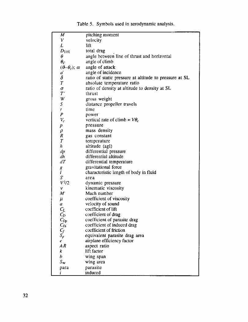
Table 5. Symbols used in aerodynamic analysis.
M
VL
Dtot0
Oc(0-0c); aa'
T
O"
T'
W
S
t
P
VcP
19R
T
h
tipdh
dT
gl
S'V2/2
V
M'
Pa
CLCo
CDiC:Spe
AR
k
b
Sw
parai
pitching moment
velocitylift
total drag
angle between line of thrust and horizontal
angle of climb
angle of attack
angle of incidence
ratio of static pressure at altitude to pressure at SL
absolute temperature ratio
ratio of density at altitude to density at SLthrust
gross weight
distance propeller travelstime
powervertical rate of climb = VOc
pressuremass density
gas constant
temperature
altitude (agl)
differential pressuredifferential altitude
differential temperature
gravitational force
characteristic length of body in fluidarea
dynamic pressure
kinematic viscosityMach number
coefficient of viscosity
velocity of soundcoefficient of lift
coefficient of drag
coefficient of parasite drag
coefficient of induced dragcoefficient of friction
equivalent parasite drag areaairplane efficiency factor
aspect ratiolift factor
wing span
wing area
parasiteinduced
32

CP1 Tail (_ _ (_ CP2 Tail
Thrust Line Center of Pressure
Lift
Thrust
Velocity_
Relative Wind f / _'_-----.- _
Theta c Theta
Weight
Figure 6. Forces and moments on an airplane in a steady climb.
steady flight the pitching moment, M, must be zero. This moment arises due to the fact that the
aerodynamic forces act at the center of pressure of the wing and tail surfaces and the thrust vector
does not necessarily pass through the center of mass. The moment is dependent on the angle of
attack at a given airspeed. In order for the airplane to exhibit the most stable response, an increment
in M, caused by a change in the angle of attack, should be negative. Otherwise, an unstable situation
is created where the airplane tends to move even farther from a steady-state condition when dis-turbed.
A. Equilibrium Flight and Airspeed
The vector sum of all the forces represented in figure 6 must equal zero for the airplane to be
in equilibrium. Therefore, the sum of forces in the direction of flight is:
T' cos (/9- Oc)-Dtot- W sin (Oc) = 0 ,
or for level flight:
(46a)
W = L and Dtot = T" (46b)
33

The vector sum normal to the direction of flight is
Wcos (Oc)-L-T" sin (O-Oc) = 0 (47)
Equations (46a) and (47) can be solved for the angle of climb by:
Oc = Tan- l {[T' cos (0- Oc) -Dtot]/[L + T" sin ((9- Oc)l ) (48)
The assumptions are made that Oc and (O--Oc) are small angles, and that the thrust for the airplane
will be only a fraction of the weight. Equation (48) now becomes:
Oc = (T'-Dtot)/W . (49)
For airplanes propelled by turbojets or rockets, equation (49) is useful in its present form. However,
the equation must be modified to deal with propeller-driven airplanes as is the case for a HASPP.
The work the propeller is capable of performing will determine the angle of climb and, in turn, the rateof climb.
In order to calculate the work the propeller performs, S is defined as the distance the propeller
travels in time t at a constant velocity V. The resultant propeller work is:
Work = T" S . (50)
Power is the rate work is performed, hence:
Powerpropener = T'(S/t) (51)
Since (S/t) is equal to velocity, the available power from the propeller is:
Pavail = T'V . (52)
By comparison, the power required by a body traveling through the air at a velocity V with a drag Dis:
Preq'd = DtotV (53)
Combining equations (49), (52), and(53) results in,
Pavail-Pre = W(VOc) (54)
The vertical rate of climb is given by (VOc) or V sin Oc = dh/dt and is referred to as Vc.
It can be seen by equation (54) that the vertical rate of climb is obtained by equating the
power required to lift the weight of the airplane at a speed Vc to the excess power. To achieve the
maximum airspeed in straight and level flight, the maximum available power must equal the power
required or:
34

Airspeedmax:eavail = ereq'd • (55)
B. Fluid Statics
An airplane's performance is related to the height at which it is flown in the standard atmo-
sphere corresponding to the pressure or density; in other words, the pressure altitude or density
altitude. The altimeter in an airplane is an absolute pressure gauge calibrated according to the stan-
dard atmosphere. Table 6 lists standard sea level values for the atmosphere. Table 7 gives values of
the standard atmosphere at 20 km (65,600 ft).
Table 6. Standard sea level values of atmosphere.
Mass density, p
Pressure, Po
Temperature, To
Kinematic viscosity, Vo
Speed of sound at sea
level, ao
0.002378 slugs/ft 3
2,116.2 lb/ft 2518.69 OR1.5723x10 -4 ft2/s
1,120 ft/s
1.223 kg/m 3101.33 kN/m 2
288.16 K
1.446x10⁻⁵ m2/s
341.4 m/s
Table 7. Standard atmosphere values
Altitude
TemperaturePressure
Mass density
Density at 60,000 ft andLatitude 40
Density at 70,000 ft andLatitude 40
Speed of Sound
Kinematic Viscosity
65,600 ft389.99 °R118.92 lb/ft 2
5.72x10 -3 lb/ft 3
2.25x 10 -4 slugs/ft 3
1.36x 10 -4 slugs/ft 3968.08 ft/s1.67x10 -3 ft2/s
20 km
216.66 K
580.58 kg/m 2
0.092 kg/m 3
116 g/m 3
70 g/m 3295.07 m/s
0.155x10 -3 m2/s
Note: The temperatures at 60,000 ft and 30 ° N. vary approximately 1 °C
from January to July, and the temperatures at 70,000 ft and 30 ° N.
vary approximately 4 °C from January to July.
A review of the relevant fluid statics relating these atmospheric values is important to an
aerodynamic analysis. Pressure, density, and temperature are examined in order to evaluate the
environment in which a HASPP will operate. The performance of a HASPP and its payload are
dependent on these conditions. The equation of state relates the pressure, density, and temperature
of a fluid by:
p = pRT, (56)
where T is the temperature in degrees K and R is the gas constant given by 287.3 m2/Ks 2 (1,545 ft-
lbf/lbmol°R) for air at normal temperatures. The variation of static pressure through the atmosphere
must be considered in order to evaluate the operating environment of the HASPP. To do this, a dif-
ferential mass of the atmosphere is examined. Summary forces on a differential mass of gas resultsin:
35
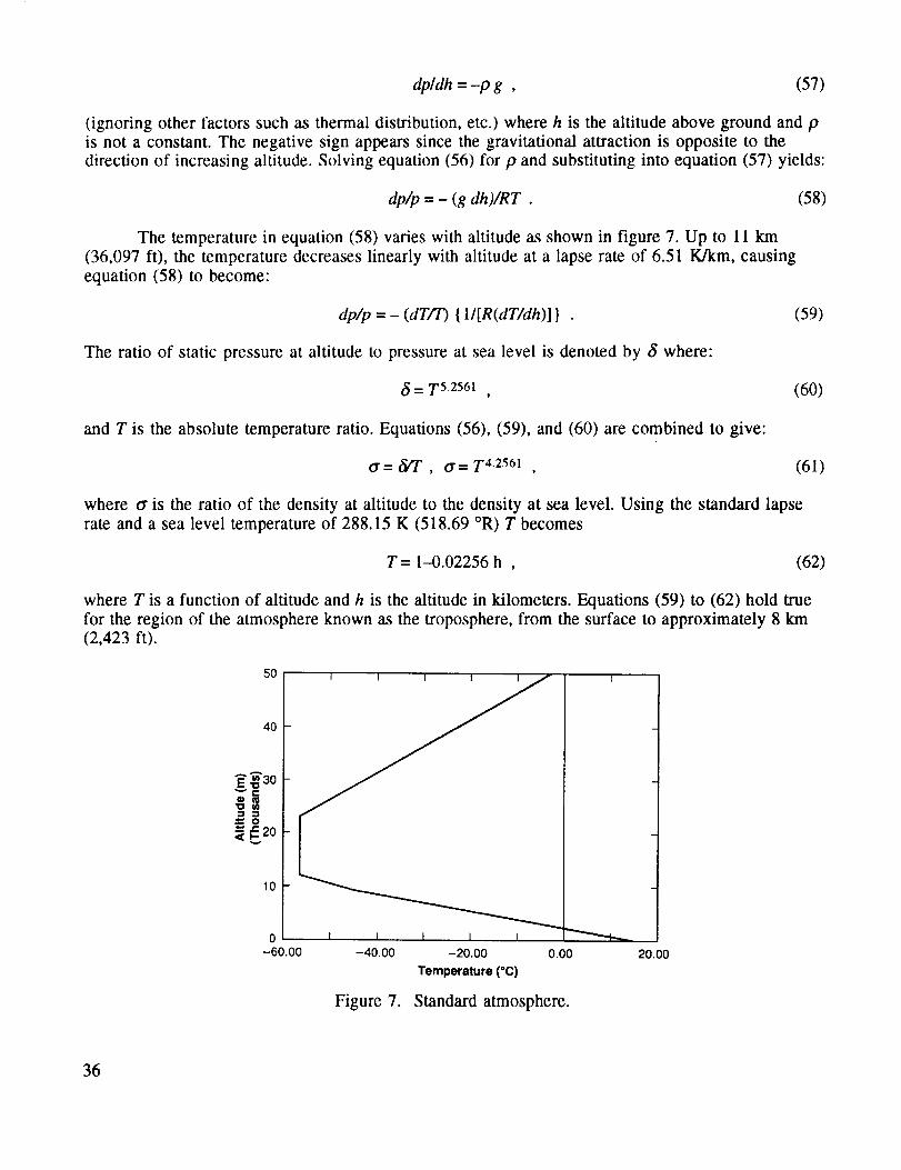
dp/dh = -/9 g , (57)
(ignoring other factors such as thermal distribution, etc.) where h is the altitude above ground and pis not a constant. The negative sign appears since the gravitational attraction is opposite to the
direction of increasing altitude. Solving equation (56) for p and substituting into equation (57) yields:
dp/p = - (g dh)/RT . (58)
The temperature in equation (58) varies with altitude as shown in figure 7. Up to 11 km
(36.097 ft), the temperature decreases linearly with altitude at a lapse rate of 6.51 K/km, causing
equation (58) to become:
dp/p = - (dT/T) { ll[R(dT/dh)] } . (59)
The ratio of static pressure at altitude to pressure at sea level is denoted by t5 where:
t_= T 5'2561 , (60)
and T is the absolute temperature ratio. Equations (56), (59), and (60) are combined to give:
O'= _/T , O'= T 4"2561 , (61)
where tr is the ratio of the density at altitude to the density at sea level. Using the standard lapse
rate and a sea level temperature of 288.15 K (518.69 °R) T becomes
T = 1-0.02256 h , (62)
where T is a function of altitude and h is the altitude in kilometers. Equations (59) to (62) hold true
for the region of the atmosphere known as the troposphere, from the surface to approximately 8 km(2,423 ft).
50
4O
= _20
10
0 I I I I I-60.00 -40.00
Figure 7.
-20.00 0.00
Temperature (*C)
Standard atmosphere.
20.00
36

At altitudes between 11 km (36,097 ft) and 23 km (75,475 ft), the temperature is approxi-
mately a constant. This region of the atmosphere is known as the lower part of the stratosphere.
Through the remainder of the stratosphere up to about 50 km (164,076 ft), the temperature increases
to approximately 270 K (486.27 °R).
C. Fluid Dynamics
A review of the relevant dynamics must now be considered for a thorough aerodynamic anal-
ysis. If the static pressure distribution normal to the surface of a body moving in a fluid is known,then the forces on the body can be determined by integrating this pressure over the surface. These
quantities are assumed to be related in the following manner:
F ~ paVblc (63)
This equation becomes:
F ~ p V212 , (64)
and:
Lift = L = (1/2) p V 2 S' CL , (65a)
Drag = D = (1]2) p V 2 S' C D , (65b)
Moment = M = (1/2) t0 V 2 S Cm , (65c)
where 12 is replaced by a reference area, S'. The quantity (pV2/2) in equations (65) is defined as the
dynamic pressure.
Some other quantities that need to be defined are the Reynolds number, Re, the kinematic
viscosity, v, and the Mach number, M'. Equations (66) define these quantities:
Re =Vlp/_= VUv, (66a)
v = p/p, (66b)
M' = V/a , (66c)
where p is the coefficient of viscosity and a is the velocity of sound. The Mach number determines to
what extent fluid compressibility can be neglected. It is interesting to note that the parasite drag
coefficient is slightly decreasing with Reynolds number. Typically it has been seen that Cop
decreases proportional to (Re)-" with n = 0.1 to 0.15 such that CDp will decrease 20 to 30 percentwith an order of magnitude decrease in Reynolds number. 38
D. Lift and Drag
The equations for lift and drag of an airplane are shown in equations (65), with CL and Co as
functions of a, the angle of attack. As stated earlier, the total drag on the plane is given as the sum
of the parasite drag and the induced drag:
37

D_t = Di+Dp_a (67)
The parasite drag, or a combination of profile drag and skin friction, is:
Opara = Cpara p/2 V 2 S" , (68)
or"
Dp_a = pl2V 2S'p_a • (69)
Where S'para = Cpara S'. S'para is the parasite area of the airplane and refers to the complete airplaneexcept the wing, while S' is the frontal area of the body. The induced drag is:
Di = p/2 V 2 CDi S t . (70)
Therefore, the total drag on a body is:
Dto t = p12 V 2 [S'wCD(Ot) + S'p] . (71)
The coefficient of drag from Youngblood's work "6
CDtot = (CDo)wing +(CDo)tail + (CDo)pod+(CDo)boom + [( 1 +,_)/(Tr *AR)]CL 2 , (27)
is a compilation of coefficients of drag for the various components of the airplane. It can be seen that
the coefficient of parasite drag for the pod, equation (25), is similar to that obtained experimentally
for an ellipsoid. 3s This report will use equations (25) and (26) for parasite drag coefficients of the
boom and pod. The wing and tail drag coefficients will be taken from drag polar charts for those air-
foils. The drag coefficient from these charts is both the parasite and induced drag for the airfoil. This
report will differ from previous designs 6 in that the tail will be considered as a lifting device as well
as the wing.
Experimental results show that the value of Cp for a rectangular plate with sides a (longerside) and b in length varied from about 1.2 at b/a -- 1.0 to 2.0 at b/a = 0. The latter point would repre-
sent a very slender rectangle. The associated Reynolds number for the experiment was about 50,000
to 150,000. Similarly, circular disks at right angles to the stream were found to have an average Cparaof 1.11. A closed hemisphere with the plane side opposed to the stream has a coefficient of parasite
drag similar to that of a circular disk, Cpara = 1.2. A circular cylinder with the stream parallel to itsaxis has a drag coefficient that is dependent on the ratio of length to diameter, l/d. The condition of
l/d = 0 is the circular disk and as I/d increased, Cpara decreases to 0.82 at l/d = 2.5 and then Cparaincreases. For Ud from 5 to 30, Cpara = 0.8 to 1.2 for Reynolds numbers below 500,000. Round bodies
(cylinders, spheres, ellipsoids, etc.) have two regions of Reynolds numbers with almost constant
values of Cpara. There is a region of transition separating moderate Reynolds and high Reynolds
numbers. Spheres, with the reference length the diameter, have a Cpara = -0.5 for Reynolds numbers
20,000 to 200,000 and Cpara = 0.2 at Reynolds numbers above 300,000. An ellipsoid with a diameterratio of I'1.8 (minor diameter vertical) at Reynolds numbers from 200,000 to 600,000 has values of
Cp_a from -0.05 to 0.1.
38
E. Airfoils
A HASPP will operate at an altitude of low density, and it will fly at speeds considered to beslow (on the order of 90 ft/s), relative to conventional airplanes. Therefore, the HASPP will operate
in a low Reynolds number regime. Based on Youngblood's 1982 design, the HASPP will operate at a
Reynolds number of approximately 3,000,000 at 20 km (65,600 ft). The HASPP presented in this
paper operates at a Reynolds number of 350,000.
Most airfoils are designed for conventional aircraft operating at higher speeds and hence for
optimal performance at higher Reynolds number range. Therefore, care must be exercised to choose
an airfoil designed specifically for high performance, slow flight, and low Reynolds numbers. It isnecessary that the airfoil used on the wings, tail, and propeller of the HASPP generate the maximum
lift and minimum drag capable of an airfoil. The maximum lift is primarily a function of the interaction
of the upper surface pressure distribution and at low Reynolds numbers, the boundary layer. The
NACA four- and five-digit airfoils were designed without consideration of the influence of the
boundary layer. The boundary layer effects were taken into consideration in design of the NACA six-
digit airfoil series. In this series, the boundary layer was considered to the extent that a boundary
layer was desired to exist over a certain laminar portion of the leading portion of the airfoil for a
specified range of lift coefficients.
The Lissaman 7769 airfoil was used on the Gossamer Condor and Gossamer Albatross. The
airfoil performed well in these applications, however, in wind tunnel tests performed after these
flights a significant degradation in performance for chord Reynolds numbers below 150,000 was
indicated. 6° The airfoils used on Solar Challenger were the Lissaman-Hibbs 8025 and 8230 for the
wing and stabilizer respectively. The 8025 has an exactly linear last 85 percent of the upper surface,
while the 8230 also has a flat upper surface with some laminar flow on the lower surface. The Boeing
Condor uses a Liebeck airfoil with a high aft camber resulting in laminar flow over 50 percent of the
upper and lower surfaces. The airfoil has a lift-to-drag ratio of 40, similar to some high performance
sailplanes, and it continuously operates at lift coefficients up to 1.35. The airfoil is designed to
operate to these specifications at Reynolds numbers near 1 million. The propeller for the Condor was
also designed with a high aspect ratio.
Wortmann has designed a series of airfoils capable of performing in a low Reynolds number
range. An upper bound on the low Reynolds number regime is assumed to be 4X10⁶. 4° Wortmann
designed airfoils with the boundary layer consideration extended to the turbulent flow regime.
Wortmann has shown that considerable reductions in the drag coefficients can be obtained by the
use of concave pressure distributions for the pressure recovery region. Wortmann's airfoils; FX-74-CL6-140, FX-74-CL5-140, FX-72-MS-150A, and FX-72-MS-150B; all show the unusual
behavior of increasing maximum lift with decreasing Reynolds number. These airfoils have a more or
less flat forepart followed by an increased camber creating an abrupt pressure rise. 32 The first two of
these airfoils are shown in figure 8. Wortmann believes that it is possible to obtain lift coefficients
between 2.0 and 2.4 even at low Reynolds numbers of about 1 million. Figures 9 and 10 show the
drag polar for the FX 72-MS-150B, FX-74-CL5-140, and FX 74-CL6-140 airfoils. The low-drag
airfoils of Wortmann's design are notably well suited to sailplane applications. The success ofWortmann's work is revealed by a study of modern high performance sailplanes. Most of these
sailplanes employ a Wortmann airfoil. 39 The Wortmann FX 63-137 airfoil was proposed for use by
Youngblood in his 1982 and 1984 papers on solar HAPP's and is illustrated in figure 11. It was
chosen for the expected Reynolds number range of 105 to 106 . Figure 12 shows the drag polar of theFX 63-137 airfoil.
39

Figure 8. Wortmann FX 74-CL5-140; FX 74-CL6-140.
1.2CL
..... Re = 0.7x10⁶Re = 0.5x10⁶
.... Re = 0.28x10⁶
4 8 12 16 20 -4
103 C D-0.4 0.1 0.4
FX 72-MS-150B/25
x
0.5 1.0 c
4 8 12 16 20 24
Figure 9. Drag polar, Cz,(a) of the FX 74-MS-150B at Reynolds numbers of 1.5 and 3.0x10⁶.
40

CL
2.4
2.0
1.6
1.2
0.8
0.4
0.0
- -0.5
- f_[./
- , ( / -o.3
I I I I I
4 8 12 16 20
2.4
,?."2"----T
Ir
-0.8
FX 74-0L5-140
I I I I I
0.4 8 12 16 20 24
0.1 -0.0O_
Drag polar, CL((Z), and transition position of the FX 74-CL5-140 at Reynoldsnumbers of 1.0, 1.5 and 3.0x10⁵.
CL
2.4
2.0
1.6
1.2
0.8
0.4
0.0
I
4
-0.5
=,,. = e-- ='=" -- =_j
•"7_,' "...... -0.4LDS _ ##
,.'/!.,' (/ -0.3i t/, (,! -0.2% \"_
, \ \ -0.1.'
I =" J t t "t.Wm
8 ""'I.2., 16 20 4:it
f'0.1J
_2.4 FX 74-0L6-140
- C L -_,,
:1v I /# )
I I I
0.4 8 12 16 20 24
(Z0.0
Drag polar, CL(Or.) and transition position'of the FX 74-CL5-140 at Reynolds
numbers of 1.0, 1.5 and 3.0x10⁶.
Figure 10. Wortmann FX 74-CL5-140, FX CL6-140.
41

Ca FX 63-137 )CaTX 63-137
1.6
1.2
0.8
0.4
0.0
...... Re = 0.7x10⁶
Re = 0.5x10⁶
Re = 0.28x10⁶
I I 1 I
4 8 12
Figure 11.
Cml/4
16 20 -4 4 8 12 16 20
103 C w
Wortmann FX 63-137.
Figure 12. Wortmann FX 63-137.
42

Chapter VIII. ENERGY STORAGE
Excess energy produced by the solar cells during peak hours of sunlight must be stored for
use at night as discussed previously. For HASPP's this energy is typically stored in either a
potential or chemical form. The flight profile using potential energy storage would consist of climbing
during the day and gliding at night. This method would fall short during the winter months when therewould not be enough daylight to enable the HASPP to climb back to its operating altitude. Chemical
storage is a better method of retaining excess energy, providing a more stable and reliable flight
profile. There are several rechargeable fuel cells available. However, energy storage continues to be
a major drawback to the feasibility of HASPP's due to their relatively great weight.
A study of fuel cells requires an understanding of some specific terminology. Table 8
comprises some of the terms and definitions common to all fuel cells.
Table 8. Fuel cell terminology. 44
(1)
(2)
(3)
(4)
(5)
(6)
(7)
(8)
(9)
(10)
A cell is the electrochemical unit used to store energy.
A battery is defined as two or more electrochemical cells electrically
connected in a series/parallel arrangement to yield the necessary
operating voltage and current levels.
The capacity of a battery is the total number of ampere-hours (Ah) that
can be withdrawn from a fully charged cell or battery.
The charge rate is the current that is applied to a cell or battery to restoreits available capacity. Usually it is normalized with respect to the rated
capacity resulting in units of amperes rather than hours.
Depth of Discharge (DOD} is defined as the percentage of Ah's with-drawn or discharged from a fully charged battery or cell.
A cycle is defined as one discharge-charge series to a specific depth of
discharge.
A battery has a cycle life, after which it fails to perform as originallyspecified. A cycle life is the number of cycles taken to a certain DOD.
When a battery has 50 percent or more of its capacity withdrawn, the
withdrawal is referred to as deep discharge.
The efficiency of a battery is the ratio of the useful output to the input.
There are Ah, voltage, and energy (watt-hour) efficiencies.
The energy density of a battery or cell is the ratio of rated energy available
normalized to its weight or volume.
43

The DOD is a direct measureof theamountof storedenergythatcanbedischargedfrom aregenerativebatterywithout decreasingthe overall efficiency.A battery'slifetime, given in termsofthenumberof charge-dischargecycles,tendsto be inverselyproportionalto the DOD.
There areseveraltypesof batteriesthat shouldbegivenconsiderationfor the HASPPapplication,keepingin mind that a high energydensityis necessaryto accomplishlow-wing loading.The leading batteriesare lead-acid,silver-zinc, silver-cadmium,nickel-hydrogen,and nickel-cadmium.The last four are listedin orderof decreasingenergydensity.All of thebatteriesmentionedarecapableof beingrechargeable,necessarydueto the long durationof theflight.
Roy Lanier of MSFC estimatesthat deepdischargebatterieswill benecessaryfor thelightest weight possible.49The depthof dischargewill needto beon theorder of 75 to 80 percent.Also it is believedthat silver-zinc batterieswill not last long at high DOD's. This indicatesthatsilver-zinc might not be usefulin this applicationor that larger thannormalsilver-zinc batterieswould needto bemadefor HASPP's.49
A. Lead-Acid Batteries
Lead-acid storage batteries have been in use for over 100 years and much research has goneinto their development. This is a lead/sulfuric acid/lead dioxide system that goes through a reaction
characterized by the double-sulfate theory. In general, the performance of lead-acid batteries
decreases with decreasing temperature and improves with increasing temperatures.
Outgassing occurs during charging of lead-acid batteries. Both hydrogen and oxygen are
emitted, particularly at high levels of charge. Sulfation, defined as the growth of lead-sulfate crystals
on the battery plates, is possible when the battery is in operation for several days continuously
without obtaining a 100 percent state of charge. The lead-sulfate crystals increase the internalresistance of a cell resulting in lower discharge and higher charge voltages.
Lead-acid photovoltaic batteries have rated capacities ranging from 26 to 3,000 Ah. The
capacity can vary during the lifetime of a battery depending on the discharge rate, the cutoff voltage,the operating temperature, the age of the battery, and the sulfation that occurs. Table 9 lists some of
the characteristics of photovoltaic lead-acid batteries.
Table 9. Lead-acid battery (1982).
Cell Type Low Rate Low Rate Medium RaI¢ Medium Rate
Capacity (Ah) 200 3,000 45 935
Rate (h) 500 500 8 8
Dimensions
LxWxH (in) 4x7xl 1 13x14x23 6x3x17 13x7x23
Weight (lb) (kg) 35 (15.89) 315 (143.01) 170 (77.18) 1,020 (463.08)
44

B. Nickel-Cadmium Batteries
Nickel-cadmium (Ni-Cd) batteries came into use around the year 1900. Rechargeable Ni-Cd
batteries have been used for two decades in spacecraft. These batteries have the advantage of a
relatively long life, however, their low capacity rating could hinder their use in photovoltaic
applications. Nickel-cadmium batteries have high rate capabilities and the ability to withstand an
overcharge. They are also more tolerant of low operating temperatures and operation at partial
states of charge than lead-acid cells. The rated capacities of Ni-Cd batteries range from 0.1 to about
23 Ah at a 5-h discharge rate. Sealed pocket plate types have about a 70 Ah capacity. The batteries
typically provide about 1,000 Wh/ft 3 (watt-hours per unit volume).
C. Nickel-Hydrogen Batteries
Nickel-hydrogen (Ni-H2) batteries have been under development by the U.S. Air Force for
10 years. In 1977 the U.S. Navy launched the Navigation Technology Satellite-2 that employs recharge-
able Ni-H2 batteries. In 1982 Ni-H 2 required 1.5 to 2,0 times the volume of an equivalent Ni-Cd
battery. Ford Aerospace Corporation has tested an 81 Ah Ni-H2 battery. The battery assembly has a
mass of 110 kg (242 lb) with each cell limited to 2.15 kg (4.76 lb) in weight and 34.3 cm (13.5 in) in
length. The cell diameter is 8.92 cm (3.51 in). The battery has a nominal DOD of 35 percent. The
average discharge voltage is 37.5 V minimum, and the battery has a design life of 38,000 cycles.
The space station photovoltaic electric power system will rely on power generated by planar
solar arrays with energy storage provided by Ni-H2 batteries. The proposed system contains 20
batteries of 90 cells packaged as 30-cell assemblies. The basic space station power requirement at
load is 75 kW (100 hp), therefore nearly 90 kW (120 hp) of dc power production capability is required
of the battery system. This requirement allows for inverter and distribution efficiencies, margins, and
fixed loads such as control microprocessors. A total peak power of 130 kW (174 hp) capability isrequired.
A typical method used for designing battery systems for space applicatons was provided by
Jeff Brewer 46 of MSFC. This method can be adapted for use in designing the energy storage system
in the HASPP. Following is an example of a battery system design to be used as a model for the
actual HASPP requirements. The model utilizes current Ni-H2 technology as applied to the Hubble
space telescope (HST).
The system requirements call for a 1-year life in a geosynchronous orbit, a battery load of 8.3
kW during a 13.2-h eclipse, and a 105-Vdc battery system. An operating voltage of 1.3 V/cell is
used to provide a conservative estimate of battery requirements. The voltage per cell is dependent
on the rate of discharge. For this application close to 1.5 V/cell is possible. This operating voltage is
used to determine the number of ceils needed to produce 105 V by:
(105 V)/(1.3V/cell) = 81 cells. (72)
The 81 cells will be connected in series in three 27-cell batteries. Typically a battery contains 24 to
32 V. The three batteries will make one module. The capacity of each cell is 90 Ah, and, since a
module consists of a series of cells, each module is capable of 90 Ah. A DOD of 80 percent per orbit
is assumed, yielding 72 Ah from each module. A constant current load of 79 A is obtained by:
(8,300 W)/(105 V) = 79 A. (73)
45

Thecapacityrequirementperorbit is calculatedfrom:
(79A)(13.2h) = 1,043Ah. (74)
To determinethe modulesrequiredto supply this capacityrequirement:
(1,043Ah)/(72Ah) = 15modules. (75)
A very conservativedesignwould includetwo additionalmodulesto protectagainstfailure. Eachofthe 17moduleswill weigh approximately515lb for a totalsystemweightof 8,755lb. Eachmoduleisapproximately45 in long,32 in wide, and15in high.This is obviouslytoomuchweight for theHASPPto carry.
D. Silver-Zinc Batteries
Silver-zinc (Ag-Zn) batteries are being tested for use in orbiting spacecraft. The Ag-Zn
combination is still in the experimental stage and the batteries are primarily nonrechargeable;
however, some rechargeable cells are being produced. Ag-Zn batteries have a higher voltage even
at lower temperatures and three times the energy density of the nickel couples. Table 10 lists the
energy densities of the most efficient rechargeable fuel cells.
The Ag-Zn cells are not capable of deep DOD's for many cycles. For this reason, it is mainly
considered a good primary battery and generally not a rechargeable battery. There is a Ag-Zn
battery system proposed for use in an 18-month life application. However, it will have only 15 deep
discharges of 70 percent. The batteries will be cycled between these deep discharges at just a
1-percent DOD. It is not recommended that a Ag-Zn system be used in this application. It has not
been done, but it is assumed possible to design a mixed system where Ag-Zn modules would beused during the summer season, when the DOD would be least.
Table 10. Rechargeable batteries.
System
Ni-Cd
Ni-Cd
Ag-Zn
Ag-Zn
DischargeVoltage
1.21
1.25 at 10 °C
1.501.44/ 1.51
Cell Energy
Density (Wh/lb) Efficiency DOD
18-23
11.0 (storage 1982)6.6 (usable)
24-26
13.0 (storage (1982)10.4 (usable)
60
77
0.8 0.60
0.8 0.80
46
E. Fuel Cells
A fuel cell is similar to conventional storage batteries in that it is a simple device that
continuously converts energy from chemicals directly into electrical energy. This electrochemical
reaction directly produces a flow of electric current upon demand. Fuel cells have higher energydensities and higher efficiencies than batteries. Furthermore fuel cells do not wear out as batteries
do. A regenerative fuel cell system weighs 25 to 50 percent less than batteries and a deep dischargeapparently has no ill effect on its performance. Realistic operating efficiencies lie between 45 and 85
percent. Tom Maloney of Sverdrup 43 indicates that an efficiency of 65 percent is commonly used in
current design practice.
A fuel cell was used as the primary source of electrical power on the Gemini and Apollo
manned space programs and has been used on the space shuttle orbiter. The fuel cells proposed for
use on the future Martian mission are designed for an energy density of 500 Wh/kg (226.9 Wh/lb).
The fuel cells will cycle at 14 h of daylight and 14 h of dark. These cells are scheduled to be in use in
about 4 to 5 years. The state of the art in fuel cells has an energy density of about 300 Wh/kg (136.2
Wh/lb) for the Martian duty cycle.
Two chemicals are used in a fuel cell; one is a fuel and the other is an oxidant. The electrolyte
cell of a fuel cell is supplied continuously with chemicals that are stored outside the cell. A commoncombination used in fuel cells is hydrogen-oxygen (H2-O2). The H2 and 02 react electrochemically
producing electrical power and water. There are several types of fuel cells available. Instead of using
hydrogen as the fuel; propane, butane, carbon monoxide, or zinc could be used. The oxygen could be
taken from the atmosphere instead of stored in a tank. There are also a variety of electrodes
available. Youngblood's solar HAPP design called for regenerative alkaline fuel cells with a nominal
time of discharge of 13.2 h. The H2-O2 thermochemical reaction (combustion) is highly exothermic.The combination has a free energy of reaction (more energy produced than taken) of 50,900 Btu/lb of
H2. Catalysts are used to reduce the energy needed to start the reaction. The catalysts are then
regenerated back to their original form. A fuel electrode catalyst can be very helpful for operations in
low temperatures. The catalyst splits the fuel molecule allowing the smaller particles to travel to thecathode. The combination of H2 and Oz can also be thermochemical (releasing heat and explosive
work) rather than electrochemical (releasing electrical energy). In an electrochemical reaction,ionization occurs, and an atom or molecule gains or loses electrons.
An example of a typical system is an H2-O2 fuel cell using an acid electrolyte. H2 gas ionizesat the fuel electrode (anode) creating H2 ions and electrons. These electrons flow away from the
anode by means of the external circuit through the electrolyte. 02 gas reacts with these H2 ions andelectrons from the circuit at the oxidant electrode (cathode). Water is produced by this reaction.
The space shuttle uses H2-O 2 fuel cells of 0.9 V/cell at 150 m]ft 2 with 0.7 to 1 ft z of planar
area. A 12.5-kW power plant weighs 210 lb without the reactants. It is 35 by 33 by 31 cm (13.8 by
13.0 by 12.2 in) which consists of 2 stacks of 32 cells connected in parallel.
In order to calculate the weight of the reactants, the energy being stored in the fuel cells must
be known. That energy would be the propulsion power plus the avionics power in watts. The number
of electrons, or moles, of H2 and 02 are calculated from:
nil2 = (It)/(2F), (76a)
47
no2 = (It)/(4F), (76b)
where I is the current in amps, t is the time of discharge or operation of the fuel cell in seconds, F is
Faraday's constant, 96,500 coulombs/eq, and 2 and 4 have units of eq/mole. The current is derivedfrom:
I = P/E (for dc), (77)
where P is the storage power in watts and E is the chosen system voltage. It will be assumed that
an extra 10 percent of each gas will be stored so the tanks will not be completely depleted.Difficulties could arise in exhausting a tank entirely.
From the number of moles, the weight of the stored gases can be calculated from:
WH2 = (nil2 (2 g/mole), (78a)
Wo2 = (no2)(32 g/mole). (78b)
Some things must be known about the storage conditions to continue. The storage temperature, T,
will be the temperature at altitude. The storage pressure, p, is assumed to be 2,000 psig. 43 A safety
factor, SF, on the reactant tanks should be between 1.5 and 4. The yield strength, Str, and the den-sity, p, of the Kevlar 49/epoxy tank (with 10 mm of titanium shell) are needed and assumed to be
800,000 psi and 3 to 6 g/cm 3, respectively. The perfect gas relationship:
pV- nRT, (79)
is used to determine the volumes of the stored gases. Assuming a spherical tank the radius is:
rtank = [3/(4¢r)Vtank ] 1/3 (80)
The thickness of the tank wall is: 43
twall = (SF)(p)(rtank)/[2(Str)-O.2(p)(SF)] . (81)
The weight of the tank is:
Wtank = (Surface Area)(twall)(Ptank) , (82)or:
Wtank = (4Xrtank2)(twall)(Ptank) . (83)
The weight of the entire fuel cell system consists of the tank weight, stored gas weight, electrolyzerweight, and fuel cell weight.
Fuel cells will be used in this application because of their low weight. Coupled with the rea-sonable weight of a fuel cell system that is capable of supplying the needs of the HASPP is the rea-
sonable volume of the fuel cell system. The Ag-Zn batteries have higher efficiencies, but lower
48

energydensities,hencehigherweight, andthey will not functionon this application.Practicalrechargeablebatterysystemswould weigh far morethan theentire HASPPwould weigh with a fuelcell system.
Chapter IX. PROPULSION SYSTEM
The HASPP propulsion system converts power generated by the solar cells into thrust to
propel the airplane. Earlier it was stated that the propulsion system includes the motor, controller,
inverter, reduction gearing, power conditioning, and propeller. This chapter contains information onthe motor and its associated components. The propeller is discussed elsewhere. A dc electric motor
is used to match the power output of the solar cells and fuel cells. A motor controller is required to
route the power from the solar cells and/or the fuel cells to the propeller. Because of the high rota-
tional speed of the motors, gear reduction to the propeller is necessary.
A. Motor
The performance of an electric motor is typically given in units of horsepower (hp) represent-
ing the power or rate at which work is performed. The hp unit is equivalent to:
hp = (To 09)/6,600, (84)
where To is the torque in ft-lb and o9 is the number of radians turned per second.
At present, the most efficient method of converting electric energy produced by the solar cells
into propulsive work for a HASPP is through an electric motor. Motors using rare-Earth magnets
employ electronic, rather than mechanical, commutation. This eliminates the associated electromag-netic interference present in conventional electric motors. In comparison to conventional motors, the
rare-Earth magnet motors have better response times, are more efficient, and are characterized by a
greater reliability. High shaft speeds provide the optimum operating environment for these motors,
with greatest efficiency and least weight under those conditions. Rare-Earth magnet motors appear
to be the optimum choice for use in this application.
The successful solar airplanes examined in this research have all used air-cooled high speed
permanent magnet dc electric motors. Project Sunrise used a 447.6 W (0.6 hp) permanent magnet
motor with a specific weight of 2.13×10 .3 kg/W (3.5 lb/hp). Gossamer Penguin used a dc double-
brush motor, while Solar Challenger used a 3.5 kg (7.71 lb) barium ferrite dc motor. The solar HAPP
proposed by Youngblood calls for a samarium cobalt permanent magnet motor.
The samarium cobalt magnet has a higher magnetic density than comparable magnets
although it is 10 times more expensive than the others. The samarium cobalt motors are being usedon board aircraft in alternators, accelerometers, and electric motors. A samarium cobalt dc motor has
also been designed for the electromechanical actuator on the space shuttle orbiter elevon. The motor
develops about 12,900 W (17.1 hp) at 9,000 r/min, weighs 7.79 kg (17.16 lb), and has an operating
efficiency of about 0.95. Tests have been performed on both samarium cobalt and strontium ferrite
motors at speeds up to 26,000 r/min. Both consistently performed at efficiencies greater than 0.93
and produced up to 26 kW (35 hp) of power. During some tests, the rpm was greater than 22,000 for
49
maximumpower.A typical samariumcobaltdc brushlessmotorhasa specificpowerof 2.2hp/kg(746W/lb) with anefficiency of 0.95.
A samariumcobalt motor/controllerwasdevelopedby SundstrandCorporationfor the AirForceXBQM-106 RPV. This particularmotor wascapableof generatingpoweroutputof a maximumof 7,800W (10.5 hp)and acontinuouspoweroutputof 3,700to 4,500W (5 to 6 hp). It wasa vari-ablespeedmotor with a maximumspeedof 6,700 r/min. The input voltage was rated at 105 Vdc at
no load and the maximum torque was 124.5 cm-kg (108 in-lb). The packaged motor/controller unitweighed 12.1 kg (26.7 lb). The specifications for this motor were suited to the Air Force RPV
mission, which does not necessarily meet the design requirements for the HASPP.
The Air Force RPV motor was a brushless dc design using samarium cobalt permanent mag-
nets in the rotor and three windings in the stator. The magnet polarities were radial and were bonded
to the eight flat surfaces of the high permeability rotor hub. This configuration created an eight-pole
magnetic rotor structure. The stator contained 39 slots with the coil windings connected in a 3-phase
wye form with 13 slots allocated to each phase. 5o Sundstrand Corporation has since been involved in
high altitude long endurance flight programs. They have designed a samarium cobalt motor capable ofperforming at an altitude range of 18 to 23 km (60,000 to 75,000 ft) for 3 to 9 months.
The motor/controller unit is air cooled with a maximum ambient temperature of 35 °C (120 °F)
for the Air Force RPV. Ram air flows through the controller first and then to the motor through
channels between the stator and the housing. The air flow passages allow heat to be effectivelyremoved from the motor since most of the motor heat is generated by losses in the stator. Because
of the high efficiency of the samarium cobalt rotor, losses in the rotor assembly are minimal. Thepower electronics are mounted on heat sinks to promote heat transfer. When the motor/controller
designed for the RPV was run at idle for 8 min without benefit of ram air cooling, the unit temperatureincreased only 14 °C (57.2 °F) above ambient temperature. 5o
The Air Force RPV was flown in an operating envelope of 0 to 460 m (1,500 ft) of altitude.
During flight it was seen that there was a slight lag between airspeed reaction and a change in motor
speed command. This can be explained by the inherent characteristics of the electric motor. The pro-peller will windmill after a reduction in rotational speed (r/min) is called for until the speed of the
vehicle is reduced correctly. This differs from gasoline engines because in their case the propeller
causes drag on the vehicle as the compression from the engine maintains a given propeller r/min. The
windmilling phenomenon associated with the electric motor removes this drag. However, includingpower regeneration into the controller could have eliminated the windmilling effect. 5o
B. Controller
An electric controller will accompany the permanent magnet motor to enable the motor to
perform properly. A controller consists of an inverter and motor control electronics. The output fromboth the solar cells and the fuel cells is direct current. The controller converts the direct current into a
three-phase output to activate the motor. A closed loop speed control keeps output speed and inputspeed in close relation.
5O

C. Inverter
Sundstrand Corporation opted for a voltage source inverter system over the current source
system for a number of reasons, one being the limitation of voltage transients (spikes) which could
cause transistors to fail. With a voltage source system, control is furnished by pulse width
modulation of the inverter switches resulting in fewer power switches for the system. Because a
voltage source system does not have as many elements, the system will have a higher calculated
efficiency than the current source method. 5°
D. Reduction Gearing
A reduction gear from the motor will be needed for the propeller to operate at the necessary
speeds. The propellers of the Boeing Condor are driven through two-speed gear boxes in order tohave efficient operation at all altitudes. At about 43,000 ft. of altitude the Condor shifts gears. The
engine to propeller r/rain ratio is shifted from 4.5:1 to 3:1. The Condor is capable of cruise speeds in
excess of 200 knots at altitude. A well-designed gear can have an operating efficiency of at least
0.98 and reduction gear efficiencies in excess of 0.99 are not uncommon.
A crude estimation of the gear weight has been proven acceptable and is necessary due to
the lack of a detailed analysis for gear weight. The gear weight in pounds is assumed to be 0.3 times
the maximum motor horsepower. Robert Boucher designed the 27:1 reduction gear for Solar
Challenger which weighed 0.68 kg (1.5 lb) for a maximum motor power of 4.1 kW (5.5 hp). The crudeweight estimation presented above is within 0.14 kg (0.3 lb) of Boucher's design. A typical gear
design for a samarium-cobalt motor has a specific power of 7.27 hp&g (2,461 W/lb) with a gear effi-
ciency of 0.99. A typical dc motor and gear system has a specific power of 573 W/lb with an efficiencyof 0.94.
E. Power Conditioning
The general electronics needed to support and integrate the flight systems should also be
considered in the propulsion system weight estimation. A variety of terms are used to signify these
fuses, switches, circuit breakers, inverters, and transformers such as: power conditioning, con-trolling, and processing. Typically the weight of the power conditioning required is based on the total
amount of power to be managed. In 1978, the power conditioning technology was at a rate of about23 W/lb. In 1980, the power processing technology at about 49 W/lb and the power control technol-
ogy at about 0.90. A schematic of the HASPP power system is shown in figure 13.
F. System Efficiency
In order to derive a propulsion system efficiency, the efficiencies of the various components
are multiplied together. These components are illustrated by figure 13 and their efficiencies are listed
in this chapter (with the propeller efficiency of the Boeing Condor) as: motor, 95 percent; reduction
gear, 99 percent; power conditioning, 90 percent; and propeller, 90 percent. Thus, the propulsion
system efficiency is 76.18 percent.
There is really no alternative to the rare-Earth magnet motors on a HASPP. Likewise, the
samarium-cobalt motor is the choice of the rare-Earth magnet motors because of its efficiency, reli-
ability, and the research that has gone into these motors for RPV's.
51
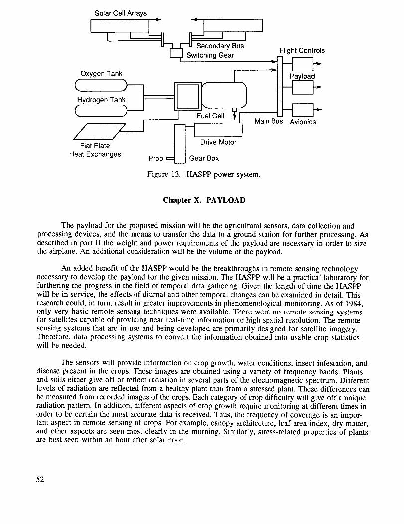
Solar Cell Arrays
Secondary Bus
Switching Gear
Oxygen Tank
_ydrogen Tank_
/ / IFlat Plate
Heat Exchanges
Fuel Cell
_ Drive Motor
Prop _ Gear Box
Main Bus
Figure 13. HASPP power system.
Flight Controls
Avionics
Chapter X. PAYLOAD
The payload for the proposed mission will be the agricultural sensors, data collection and
processing devices, and the means to transfer the data to a ground station for further processing. As
described in part II the weight and power requirements of the payload are necessary in order to sizethe airplane. An additional consideration will be the volume of the payload.
An added benefit of the HASPP would be the breakthroughs in remote sensing technology
necessary to develop the payload for the given mission. The HASPP will be a practical laboratory forfurthering the progress in the field of temporal data gathering. Given the length of time the HASPP
will be in service, the effects of diurnal and other temporal changes can be examined in detail. This
research could, in turn, result in greater improvements in phenomenological monitoring. As of 1984,
only very basic remote sensing techniques were available. There were no remote sensing systemsfor satellites capable of providing near real-time information or high spatial resolution. The remote
sensing systems that are in use and being developed are primarily designed for satellite imagery.
Therefore, data processing systems to convert the information obtained into usable crop statisticswill be needed.
The sensors will provide information on crop growth, water conditions, insect infestation, and
disease present in the crops. These images are obtained using a variety of frequency bands. Plants
and soils either give off or reflect radiation in several parts of the electromagnetic spectrum. Different
levels of radiation are reflected from a healthy plant that, from a stressed plant. These differences can
be measured from recorded images of the crops. Each category of crop difficulty will give off a unique
radiation pattern. In addition, different aspects of crop growth require monitoring at different times in
order to be certain the most accurate data is received. Thus, the frequency of coverage is an impor-
tant aspect in remote sensing of crops. For example, canopy architecture, leaf area index, dry matter,
and other aspects are seen most clearly in the morning. Similarly, stress-related properties of plantsare best seen within an hour after solar noon.
52

Occasionally,farmerswill currentlyusecolor infraredphotographyto analyzetheir crops.Ordinary vision and film aresensitiveto just a small frequencybandwithin the electromagneticspec-trum; however,color infraredphotographycapturesanotherband.Eachwavelengthgivescertain dataoncropsand soils. The wavelengthsthat canbe sensedpassively(photography)canbe recordedon mag-netic tape.The wavelengthsthat aresensedactively (radarbeam)have the reflected imagesrecorded.In the 1960"s,imagesin thevisible, nearinfrared,andthermalinfraredradiation wavelengthbandswereavailable from airbornesensors.Multispectral scannersflown over agricultural areasprovedthat thewater contentof thesoil canbedeterminedthroughtheemissionof thermalinfraredradiation.Someofthe visible and near-infrared bands were able to distinguish vegetation. The portable radiometer, used
to gather ground data is an aid to satellite imagery. By the mid-1970's, radiometers were hand held orboom mounted. These radiometers measured emitted radiation, with an 8- to 14-micrometer band lead-
ing to plant and soil temperatures. There are also radiometers that measure visible, near-infrared, infra-
red, and thermal bands. The spectrometer is another device used in agricultural monitoring. Ten years
ago a backpack spectrometer weighed about 65 lb, today it is hand held and weights 5 lb.
An agricultural sensor on a HASPP should operate similarly to the thematic mapper on
Landsat-4. The sensor should operate in five wavelength bands comparable to bands 2, 3, 4, 5, and 6
on Landsat. These bands correspond to the frequencies: 0.52 to 0.60 micrometers, 0.63 to 0.69
micrometers, 0.76 to 0.90 micrometers, 1.55 to 1.75 micrometers, and 0.40 to 12.5 micrometers. Afarm with a minimum field size of about 40 acres (161,880 m 2) and uniform soils can use a sensor
resolution of 30 by 30 m (98.4 by 98.4 ft) corresponding to the thematic mapper. However, most
fields are not this large and soils are not usually very consistent throughout a field. For a typical
field, the best resolution would be 5 by 5 m (16.4 by 16.4 ft) up to a maximum acceptable resolution
of 20 by 20 m.
The first scanning bands, red and near infrared, corresponding to bands 3 and 4 of the
thematic mapper show the amount of green vegetation present. Through these, the crop growth can
be monitored and the crop yield projected. The sensor bands providing thermal images give data on
the water condition of crops. The 1.55 to 1.75 micrometer band is sensitive to plant canopy as well as
the water content of the plants. If this band is combined with other bands, then the net radiation
absorbed by the crops can possibly be estimated. From this, the amount of water transpired can be
estimated, thus the amount of water used by the crops. The visible wavelengths show mineral defi-
ciencies by an increase in the reflectance of radiation.
A possible remote sensing method for the future is laser-induced fluorescence (LIF).
Nutrient deficiencies can be detected in crops with the pulsed nitrogen laser. Deficiencies in phos-
phorous, nitrogen, and iron can be detected through a decrease in fluorescence at 0.69 and 0.74
micrometer. An increase in fluorescence indicates a lack of potassium. Past and current methods of
remote sensing of plants typically can not identify the particular nutrient that is deficient. The LIF
could be a solution to this problem.
A sensor package that has flown on the C-130 and on the U-2 is the advanced solid-state
array spectraradiometer (ASAS). The ASAS is designed for a variety of missions, but it has flown
agricultural monitoring missions over Kansas and for the forest ecosystem over Maine. For design
purposes, the ASAS will be the assumed payload in the HASPP.
The ASAS has 32 spectred channels, corresponding to wavelengths in the visible and near-infrared range. The array of detectors is 512 by 32 or 16,384 detectors. Each spectral channel sees 14
nanometers, therefore, it ranges from 440 to 855 nanometers. The ASAS has a field of view of 25 °
53
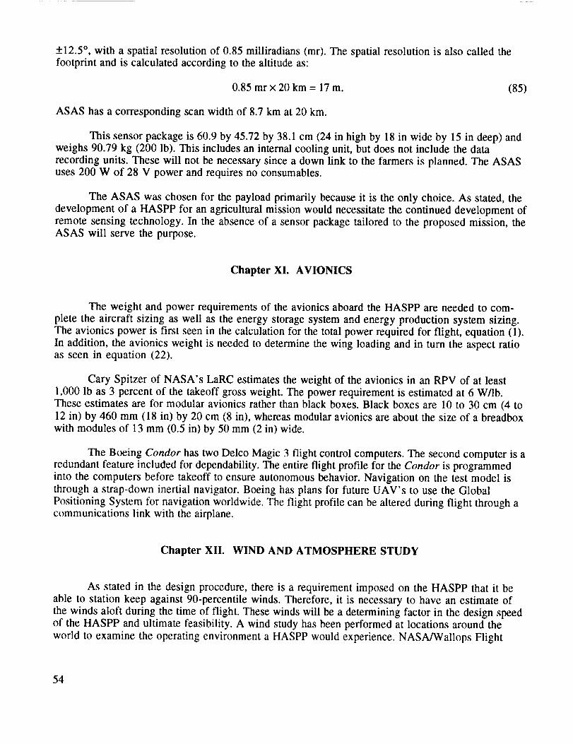
+12.5 °, with a spatial resolution of 0.85 milliradians (mr). The spatial resolution is also called thefootprint and is calculated according to the altitude as:
0.85 mr x 20 km = 17 m. (85)
ASAS has a corresponding scan width of 8.7 km at 20 km.
This sensor package is 60.9 by 45.72 by 38.1 cm (24 in high by 18 in wide by 15 in deep) and
weighs 90.79 kg (200 lb). This includes an internal cooling unit, but does not include the data
recording units. These will not be necessary since a down link to the farmers is planned. The ASASuses 200 W of 28 V power and requires no consumables.
The ASAS was chosen for the payload primarily because it is the only choice. As stated, the
development of a HASPP for an agricultural mission would necessitate the continued development ofremote sensing technology. In the absence of a sensor package tailored to the proposed mission, the
ASAS will serve the purpose.
Chapter XI. AVIONICS
The weight and power requirements of the avionics aboard the HASPP are needed to com-
plete the aircraft sizing as well as the energy storage system and energy production system sizing.The avionics power is first seen in the calculation for the total power required for flight, equation (1).
In addition, the avionics weight is needed to determine the wing loading and in turn the aspect ratioas seen in equation (22).
Cary Spitzer of NASA's LaRC estimates the weight of the avionics in an RPV of at least
1,000 lb as 3 percent of the takeoff gross weight. The power requirement is estimated at 6 W/lb.
These estimates are for modular avionics rather than black boxes. Black boxes are 10 to 30 cm (4 to12 in) by 460 mm (18 in) by 20 cm (8 in), whereas modular avionics are about the size of a breadbox
with modules of 13 mm (0.5 in) by 50 mm (2 in) wide.
The Boeing Condor has two Delco Magic 3 flight control computers. The second computer is a
redundant feature included for dependability. The entire flight profile for the Condor is programmed
into the computers before takeoff to ensure autonomous behavior. Navigation on the test model is
through a strap-down inertial navigator. Boeing has plans for future UAV's to use the Global
Positioning System for navigation worldwide. The flight profile can be altered during flight through acommunications link with the airplane.
Chapter XII. WIND AND ATMOSPHERE STUDY
As stated in the design procedure, there is a requirement imposed on the HASPP that it beable to station keep against 90-percentile winds. Therefore, it is necessary to have an estimate of
the winds aloft during the time of flight. These winds will be a determining factor in the design speedof the HASPP and ultimate feasibility. A wind study has been performed at locations around the
world to examine the operating environment a HASPP would experience. NASA/Wallops Flight
54
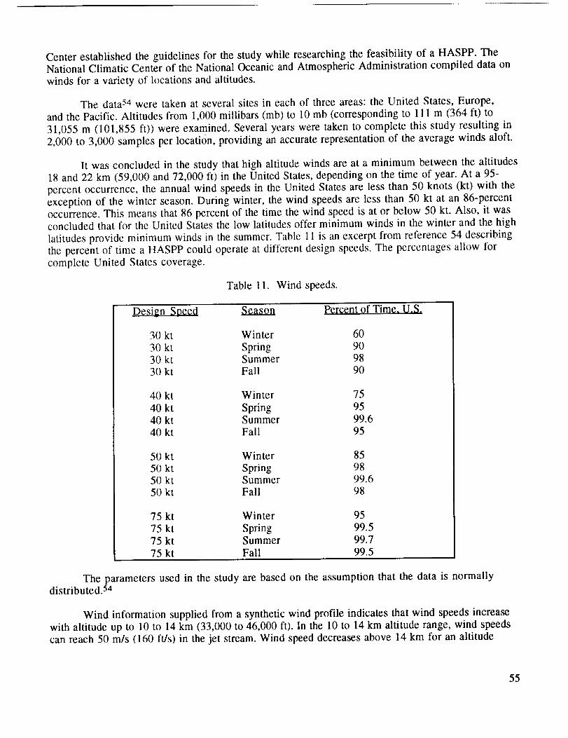
Centerestablishedthe guidelinesfor the studywhile researchingthe feasibility of a HASPP. TheNational Climatic Center of the National Oceanic and Atmospheric Administration compiled data on
winds for a variety of locations and altitudes.
The data 54 were taken at several sites in each of three areas: the United States, Europe,
and the Pacific. Altitudes from 1,000 millibars (mb) to 10 mb (corresponding to 111 m (364 ft) to
31,055 m (101,855 ft)) were examined. Several years were taken to complete this study resulting in
2,000 to 3,000 samples per location, providing an accurate representation of the average winds aloft.
It was concluded in the study that high altitude winds are at a minimum between the altitudes
18 and 22 km (59,000 and 72,000 ft) in the United States, depending on the time of year. At a 95-
percent occurrence, the annual wind speeds in the United States are less than 50 knots (kt) with the
exception of the winter season. During winter, the wind speeds are less than 50 kt at an 86-percent
occurrence. This means that 86 percent of the time the wind speed is at or below 50 kt. Also, it wasconcluded that for the United States the low latitudes offer minimum winds in the winter and the high
latitudes provide minimum winds in the summer. Table 11 is an excerpt from reference 54 describing
the percent of time a HASPP could operate at different design speeds. The percentages allow for
complete United States coverage.
Table 11. Wind speeds.
Design Speefl Season Percent of Time. U.S.
30 kt Winter 60
30 kt Spring 9030 kt Summer 98
30 kt Fall 90
40 kt Winter 75
40 kt Spring 9540 kt Summer 99.6
40 kt Fall 95
50 kt Winter 85
50 kt Spring 9850 kt Summer 99.650 kt Fall 98
75 kt Winter 95
75 kt Spring 99.575 kt Summer 99.7
75 kt Fall 99.5
The parameters used in the study are based on the assumption that the data is normallydistributed. 54
Wind information supplied from a synthetic wind profile indicates that wind speeds increase
with altitude up to 10 to 14 km (33,000 to 46,000 ft). In the 10 to 14 km altitude range, wind speeds
can reach 50 m/s (160 ft/s) in the jet stream. Wind speed decreases above 14 km for an altitude
55

rangeand then increasesagain.Anothersourceon winds indicated that mean winds in January at
120 ° W. longitude and 40 ° N. latitude are 46 kt at 60,000 ft and 28 kt at 70,000 ft. In July at 60,000 ft,the mean winds are 3 kt and at 70,000 ft 14 kt.
The data presented in figures 14 through 21 are taken from figures presented in reference 54.
Only selected sites around the San Joaquin Valley are examined, just as the only altitudes of inter-
est are 50 and 60 mb, corresponding to 64,000 and 68,000 feet, surrounding the design altitude of 20
km (65,600 ft). From figures 14 to 21, it is estimated that at least 90 percent of the time the wind
speed in the vicinity of the San Joaquin Valley at approximately 20 km (65,600 ft) will be 30 kt (50.6ft/s) or less.
Wind gustiness, or the wind variability over time intervals as short as a few seconds, exists
at all altitudes in the atmosphere. The amplitude of the gusts decrease with increases in altitude andgusts at the HASPP operating altitude can be neglected with reasonable accuracy. 56
A study of the atmosphere is necessary to determine the environment in which the HASPP
will operate. The solar radiation has been discussed in chapter IV, while the atmosphere content willbe examined here.
5O
45 -
40
,-.. 35-
30 -
Q.0_-o 25-c
.m
20-
15-
10-
52O
Wind Speed at AltitudesI I I I 1 I
Mean Speed ..........
95 Percentile
99 Percentile
f
JJ
ff
I 1 I I I
Figure 14.
40 60
Pressure (rob)
Wind speeds, Oakland, CA, spring.
80
56
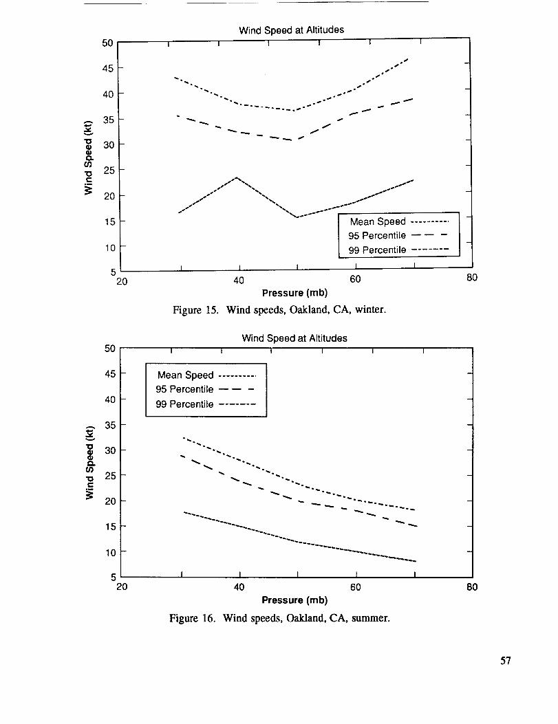
50
45
40
,-, 35
"O 30G)
"o 25C
N 20
520
Wind Speed at AltitudesI I I I I
•.,. f
. o
95 Percentile
99 Percentile -
I 1 I I I
40 60
Pressure (mb)
Wind speeds, Oakland, CA, winter.Figure 15.
8O
5O
45-
40
.-.. 35-
30-
•_ 25-C
om
20-
15"
10"-
52O
Wind Speed at AltitudesI I I I I I
Mean Speed ..........
95 Percentile
99 Percentile
"- -'22y- .
I I I I
40 60
Pressure (mb)
Figure 16. Wind speeds, Oakland, CA, summer.
8O
57
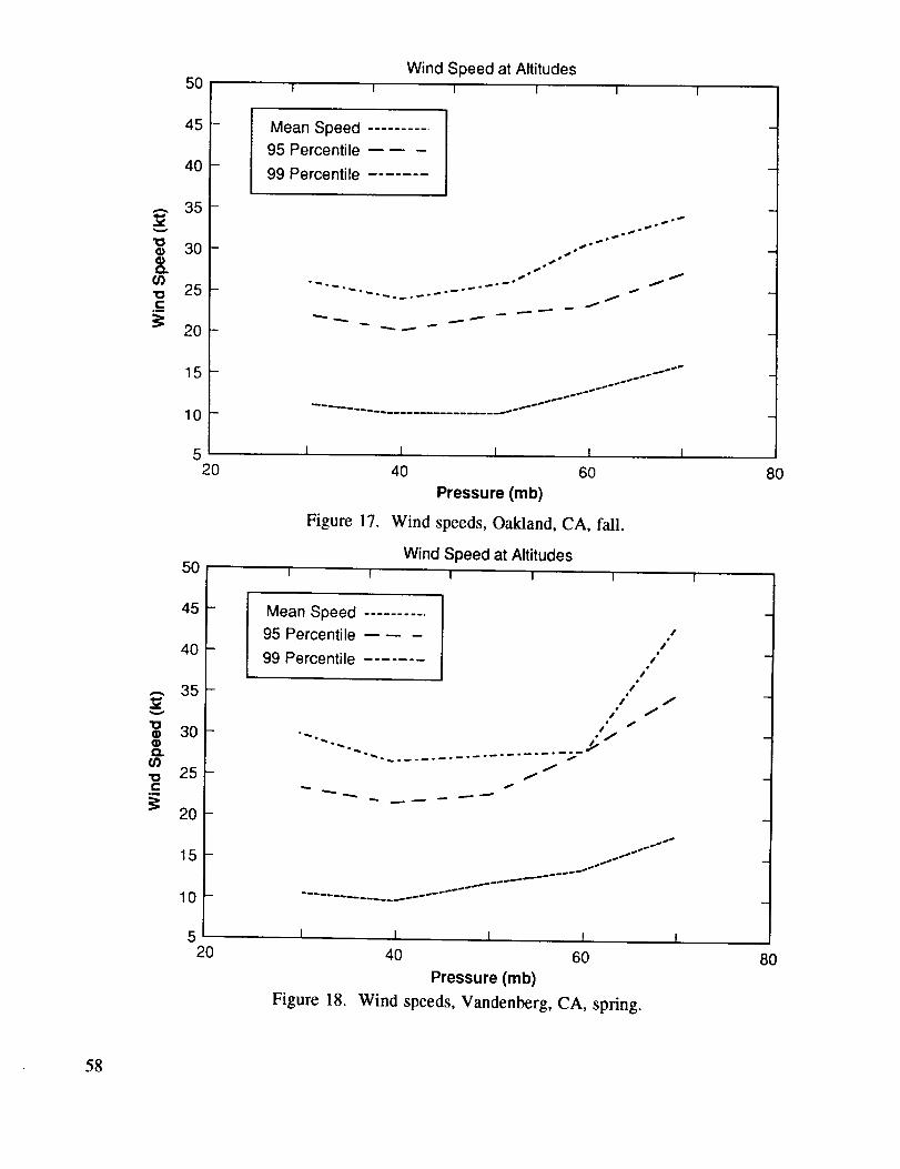
5O
45
40
,-, 35-
30-tt-o 25-c
20-
15-
10-
52O
5O
45
4O
.-. 35
a0-e_
-o 25-c
2o-
15-
10-
52O
Wind Speed at AltitudesI I I I I I
Mean Speed ..........
95 Percentile
99 Percentile
, o_,J.
S °
_ _°__B_° _
I t I I I
40 6O
Pressure (rob)
Figure 17. Wind speeds, Oakland, CA, fall.
Wind Speed at AltitudesI I I | I I
Mean Speed ..........
95 Percentile
99 Percentile
,t •
_i /
s
I
$*
I
S •e
s ff
w"
.. _°_'_
Figure 18.
I I I
40 60
Pressure (rob)
Wind speeds, Vandenberg, CA, spring.
80
8O
58
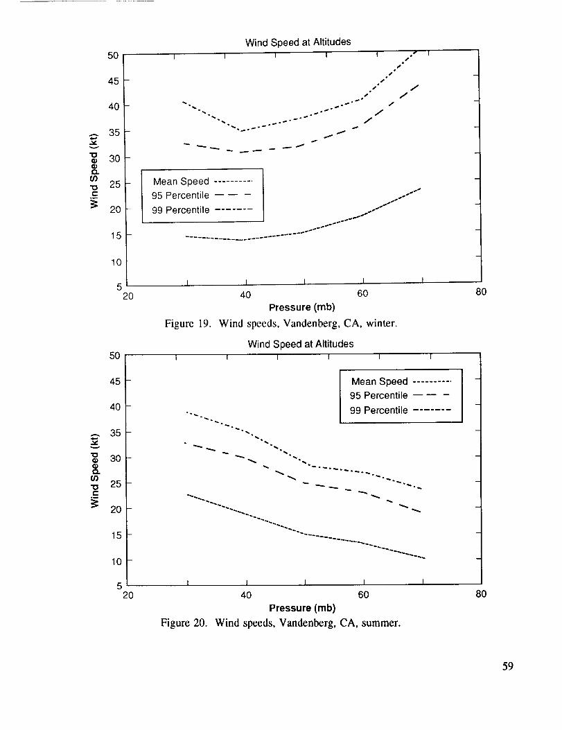
50
45
40
.-. 35
v
"O30
Q.
•_ 25t-,
Q_
N 20
15
5120
50
45
40
35
"_ 3o
_ 2o
15
10
Wind Speed at Altitudes[ I I I I
j,
S
"'° f
J
f
4.S
j.
JJ
Mean Speed ..........
95 Percentile .,.,,.--"
99 Percentile .,...f ''/
I I I 1 I
40 60
Pressure (rob)
Wind speeds, Vandenberg, CA, winter.
Wind Speed at Altitudes
Figure 19.
I I I I I I
Mean Speed ..........
95 Percentile
•...... 99 Percentile
52O
I I ! I I
Figure 20.
40 60
Pressure (mb)
Wind speeds, Vandenberg, CA, summer.
80
80
59

5O
45
4O
,-. 35
"O_) 30,&
(/1._ 25-i,-
20-
15-
10-
Wind Speed at AltitudesI I I I 1 I
Mean Speed ..........
95 Percentile
99 Percentile
_ _ °_
os
s o
I I I I I520 40 60 80
Pressure (mb)
Figure 21. Wind speeds, Vandenbcrg, CA, fall.
Atmosphere shells are regions of the atmosphere that denote specific altitudes. The tropo-
sphere extends from sea level to approximately 8 km (5 mi). All weather occurs in this region which
is subject to convection from the Earth. The lower troposphere (15,500 to 45,000 ft) contains
cirriform clouds usually composed entirely of ice crystals. Here, the temperature lapse rate is mostly
uniform at 6.5 K/km. The Earth's surface extends well into the troposphere with the higher mountain
ranges; Mt. Everest peaks just before the transition into the stratosphere. The tropopause is theregion within the troposphere of high winds and highest cirrus clouds, which occurs between 6 and 8km.
The stratosphere begins at approximately 8 km (5 mi) msl (mean sea level) and ends at
around 25 km (15 mi), at the middle latitudes, however, it is thicker over the poles and thinner or
nonexistent over the equator. The stratopau_ is a region of the upper stratosphere where
atmospheric ozone is a maximum. Also found near this region are the rare nacreous clouds.
Temperatures in this region are for the most part constant at about arctic winter temperatures. As
stated earlier, winds are at a minimum in this region, from 18 to 22 km and this is the region of pro-
posed HASPP operation. Ozone, formed by the photochemical dissociation of diatomic oxygen byultraviolet radiation from the Sun, in the stratosphere increases with altitude to about 30 km and
then decreases. Maximum atmospheric ozone is about 7 to 10 parts per million by volume. A HASPP
at 20 km would be subject to the effects of ozone, 03, but not at the maximum concentration possible.
Ozone does, however, absorb ultraviolet radiation that woald be harmful to the Mylar covering of aHASPP.
Oxidizing agents such as: 03, 02, and NO2 cause rubber and plastics to become brittle and/or
crack. Ozone is particularly deleterious to rubber under tension. The detriment to plastics is
dependent on several factors including the composition of the polymer and the amount of exposure to
6O

the oxidizing agentaswell asheatandlight. Thedurationof a HASPPmissionat approximately36°latitudewould bedependenton the degradationof theMylar covering.This degradationmaybeslowedby using antioxidantswhich displaya synergisticeffect.
The amountof water vaporpresentin theatmosphereis a function of the air temperature, as
temperature decreases so does water vapor content. A negligible amount of water vapor exists at
temperatures of -40 to -50 °C. As seen in table 8, the HASPP will operate at approximately -56 °C(-70 °F), so water vapor, and hence icing and blocking of solar radiation, will not be a concern.
61

PART IlL METHOD OF ANALYSIS
In this report, a HASPP has been designed to meet the reference mission requirements. The
design methodology as stated in part II and shown in figure 1 is followed using information from
chapters II through VIII. The solar cell data (chapter V), the motor/controller characteristics (chapter
IX), and the theory behind the available energy storage mediums was explored prior to beginning theiterative design procedure. A particular type of solar cell has been chosen for use on the HASPP,
with its associated efficiency and weight input to the reference mission parameters. A samarium-
cobalt motor/controller has been chosen for the HASPP application, with the weight, efficiency, size,
and voltage of the system effecting the overall HASPP design. Similarly, the characteristics of
weight, efficiency, size, and voltage of the chosen energy storage medium are input parameters to
the design. The choice of an optimum solar cell, motor, and fuel cell has been made based on a study
of the available options presented in each section and is also dependent on information stemming
from a study of the atmospheric environment, chapters IV and XII.
The daily energy balance algorithm, illustrated by figure 2, requires a study of the solar radia-tion environment (chapter IV). A computer program has been written to describe the radiation avail-
able for the reference mission. Radiation, air mass, atmospheric transmittance, and solar cell powerare computed for each hour of each day of the mission. These data have been used to determine thefeasibility of flight during the day of least solar radiation.
The design procedure is then completed as described in part II followed by an aerodynamic
analysis of the resulting airplane. The construction details (chapter VI) are provided as an estimate
for the structural weight and to serve as a baseline for the possible development of a HASPP.
Below is a table representing the decision matrix for the HASPP subsystems. Each of these
decisions have been discussed in detail in their respective chapters. The choices listed below occurin the design in the following chapter.
Most
Comparably Lowest Expensive Highest Reliability/
Small Size Weight Choice Efficiency Durability
GaAs
Solar CellsN/A No Y e s Y e s Good
H2-O2Fuel Cells
Yes Yes No Data No Good
Samarium-
Cobalt MotorYes Yes Yes Yes Good
ASAS
Payload
Yes Yes No Data N/A Good
Modular
AvionicsY e s Y e s No Data N/A Good
62
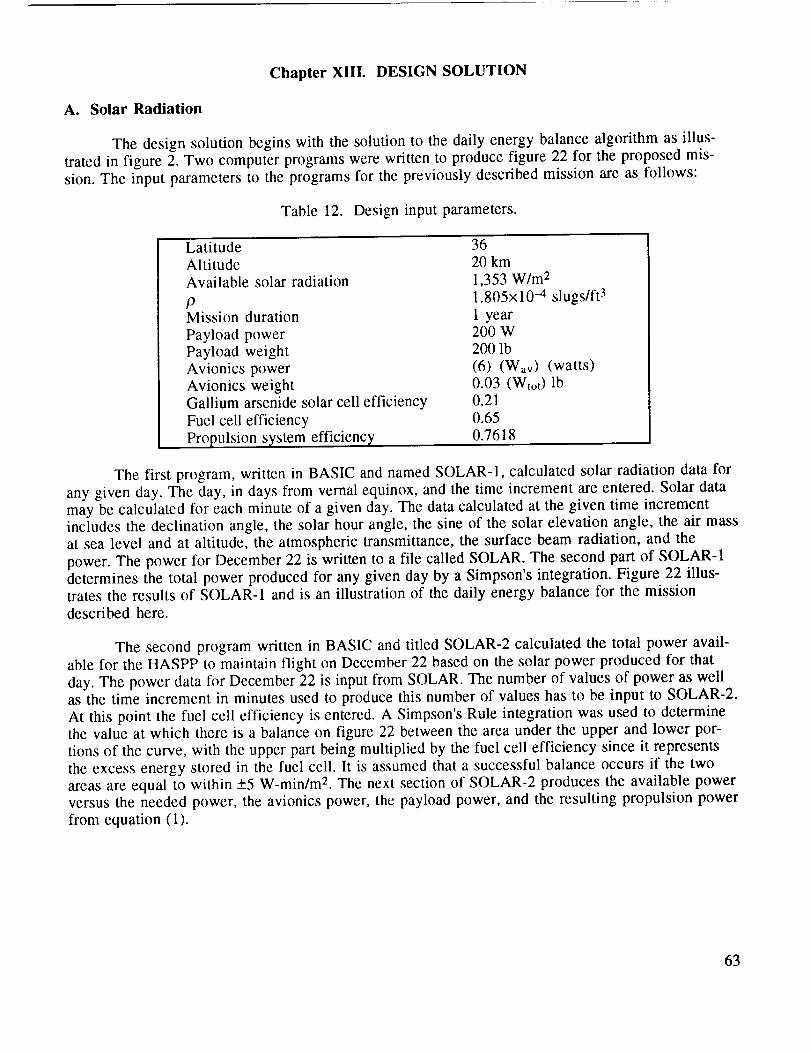
Chapter XIII. DESIGN SOLUTION
A. Solar Radiation
The design solution begins with the solution to the daily energy balance algorithm as illus-
trated in figure 2. Two computer programs were written to produce figure 22 for the proposed mis-
sion. The input parameters to the programs for the previously described mission are as follows:
Table 12. Design input parameters.
Latitude
Altitude
Available solar radiation
/9Mission duration
Payload power
Payload weight
Avionics power
Avionics weight
Gallium arsenide solar cell efficiency
Fuel cell efficiency
Propulsion system efficiency
36
20 km
1,353 W/m 2
1.805× 10 4 slugs/ft 3
1 year2O0 W
200 lb
(6) (Wav) (watts)
0.03 (Wtot) lb0.21
0.65
0.7618
The first program, written in BASIC and named SOLAR-I, calculated solar radiation data for
any given day. The day, in days from vernal equinox, and the time increment are entered. Solar data
may be calculated for each minute of a given day. The data calculated at the given time increment
includes the declination angle, the solar hour angle, the sine of the solar elevation angle, the air mass
at sea level and at altitude, the atmospheric transmittance, the surface beam radiation, and the
power. The power for December 22 is written to a file called SOLAR. The second part of SOLAR-1
determines the total power produced for any given day by a Simpson's integration. Figure 22 illus-
trates the results of SOLAR-1 and is an illustration of the daily energy balance for the missiondescribed here.
The second program written in BASIC and titled SOLAR-2 calculated the total power avail-
able for the HASPP to maintain flight on December 22 based on the solar power produced for that
day. The power data for December 22 is input from SOLAR. The number of values of power as well
as the time increment in minutes used to produce this number of values has to be input to SOLAR-2.
At this point the fuel cell efficiency is entered. A Simpson's Rule integration was used to determine
the value at which there is a balance on figure 22 between the area under the upper and lower por-
tions of the curve, with the upper part being multiplied by the fuel cell efficiency since it represents
the excess energy stored in the fuel cell. It is assumed that a successful balance occurs if the twoareas are equal to within +5 W-minim 2. The next section of SOLAR-2 produces the available power
versus the needed power, the avionics power, the payload power, and the resulting propulsion powerfrom equation (1).
63
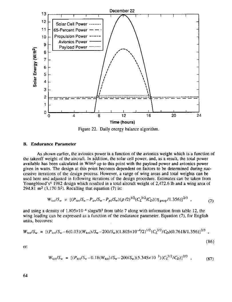
A
G)e"
Ill
Ot/}
13
12
11
10
9
8
7
6
5
4
3
2
1
0
I I 1 I
Solar Cell Power .......
65-Percent Power -- -- •
Propulsion Power .....Avionics Power
Payload Power ...........
December 22
s/
/I
II
II
II
II
II
!I
I
I 1 I 1
I I I0 4 8 12 16 20 24
Time (hours)
Figure 22. Daily energy balance algorithm.
B. Endurance Parameter
As shown earlier, the avionics power is a function of the avionics weight which is a function of
the takeoff weight of the aircraft. In addition, the solar cell power, and, as a result, the total poweravailable has been calculated in W/m 2 up to this point with the payload power and avionics power
given in watts. The design at this point becomes dependent on factors to be determined during suc-
cessive iterations of the design process. However, a range of wing areas and total weights can be
used here and adjusted in following iterations of the design procedure. Estimates can be taken from
Youngblood's 6 1982 design which resulted in a total aircraft weight of 2,472.6 lb and a wing area of294.81 m 2 (3,170 ft2). Recalling that equation (7) is:
Wtot/Sw = [(Ptot/Sw- PavlSw-PpllSw)(P 12)l/2(CL3121CD)(11 prop]l.356)] 2/3 , (7)
and using a density of 1.805x10 -4 slugs/ft 3 from table 7 along with information from table 12, the
wing loading can be expressed as a function of the endurance parameter. Equation (7), for Englishunits, becomes:
Wtot/Sw = [(etot/Sw- 6(0.03)(Wtot)/Sw- 200/Sw)(1.805x 10-4/2) I/2 (C3/2/CD)(0.7618/1.356)] 2/3
(86)
or:
Wtot/Sw = [(Ptot/Sw- 0.18(Wtot)/Sw- 200/Sw)(5.345× 10 -3) (C?I2/CD)] 2/3 , (87)
64

The total power available to maintain flight for December 22, from SOLAR-2, is:
PtotlSw = 23.285 W/m 2 = 2.165 W/ft 2 (88)
Equations (87) and (88) produce the endurance parameter as a function of wing loading. A curve of
endurance parameter versus wing loading has been generated for estimated wing loadings from
equation (89):
CL312/CD = (Wtot/Sw)312/[(5.34x 1 0 -3) (2.165-0.18 WtotlSw-2OO/Sw)] (89)
This curve is shown in figure 23. It is possible that the airplane could have sufficient energy to
maintain flight on days of low local solar radiation, but not have enough power to operate the pay-
load. This situation is represented by figure 24, noting from equation (89) that when the payload
power is removed the equation is only a function of wing loading.
L_
EtGL-
IX
o1-
"Ot-
Lid
150
140
130
120
110
100
90
80
70
December 22; Latitude 36 DegreesI I I I I
Wing Area= 800Wing Area = 900Wing Area = 1000Wing Area = 1100Wing Area = 1200 ...............Wing Area = 1300
60
50
400.6
I I I I
0.8 1.0
Figure 23.
Wing Loading
Wing loading versus endurance parameter.
I
1.2
65

L-
Et_L_
Oi-
.=1"0t-I,U
130
120
110
100
90
80
7O
60
50
400.6
Without Payload ActivatedI I I I I
All Wing Areas
0.8 1.0 1.2
Wing Loading
Figure 24. Wing loading versus endurance parameter without payload.
C. Weights
The airplane sizing algorithm, as outlined in chapter III, should be performed now. This algo-
rithm yields the aspect ratio of the wing, the wing span, and the wing area. The airframe loading ofthe HASPP is expressed by equation (22):
Waf/ Sw = Wtot/Sw - Wprop/Sw - Wsc/Sw - Wfc/Sw - Wpl/Sw - Wav/Sw • (22)
The HASPP airframe weight can be estimated by the method intended for sailplanes and modified by
Youngblood and Talay 6 12 as shown in equation (17), and the remaining components of equation (22)
can be estimated by equations (18) through (21) and the avionics weight from chapter XI as shown
at the beginning of this section. The payload weight from equation (21)6 differs from the weight given
in chapter X. A payload weight of 200 lb from chapter X is used in this analysis. Thus, equation (21)becomes:
Wpt/Sw = 2001Sw lb/ft 2 (90)
The avionics weight as discussed earlier is given as 3 percent of the takeoff weight of the aircraft or:
Wav/Sw = 0.03 Wtot/Sw • (91)
66

The airframe weight estimationof equation (17) is rewritten as an aspect ratio as shown in equation
(23). When equation (22) is substituted into equation (23), the aspect ratio is expressed as:
AR = [ (Wtot/Sw- Wprop/Sw - Wsc/Sw- Wfc/Sw- Wpl[Sw
_Wav/Sw)S°'222/(0.310 no.311)] 2.141 ,
(92)
where n, the ultimate load factor, is 4. Substituting equations (18), (19), (20), (90), (91), and To =
13.2 h into equation (92) results in:
AR = [(Wtot/Sw-O.O12 Pprop/Sw-O.15OSsc/Sw-(13.2 Ptot)/(F* Sw)-2OO/Sw
-0.03Wtot) ]Sw)Sw°'222[( 0.310*(4) TM 1)]2.141 ,
or
AR = [(0.97 Wtot-0.012 Pprop-O.15OSsc-(13.2/F)Ptot)-200)/0"477.Sw°'77812"141 (93)
By substituting the estimated specific energy of the fuel cell as given in chapter VIII, F = 300 Wh/kg
(136.2 Wh/lb), equation (93) becomes:
AR = [(0.97 Wtot-0.012 Pprop-0.15 Ssc-0.097 Ptot-200)/(0.477 Sw0.778)] 2'141 (94)
(in English units) .
This equation can be further reduced by using the relationship between solar cell area and wing area,
Ssc/Sw = 1.00, as given in chapter III. The result is:
AR = [(0.97 Wtot-0.012 eprop-0.15 Ssw-O.097 Ptot-200)/(0.477 Sw0"778)] 2"141 (95)
The propulsion power can be written as:
Pprop = Ptot-Ppl-Pav = 2.165S-200-0.18W , (96)
by combining equation (1) and information on the avionics weight and power requirements. Equation(95) can be further simplified by incorporating equation (96), the given payload power requirement of200 W, and the calculated Ptot/Sw of 23.285 W/m 2 (2.165 W/ft 2 or Ptot = 2.165 Sw W) from SOLAR-2
as"
AR = [(0.972 Wtot-0.386 Sw-197.6)/(0.477 Sw 0'778 )]2.141 (97)
D. Aerodynamics
A curve of aspect ratio versus wing area was generated and is shown in figure 25, keeping inmind that the aspect ratio is a function of the square of the wing span and the wing area as well as
being a function of wing span and wing chord. In order to reduce the wide variety of possible wing
loadings and wing areas, the aspect ratio limit of 30 is overlaid on the curves of aspect ratio versus
wing area. As mentioned earlier, it might be necessary to fly during critical days without the payload
operating. This situation would alter equation (96) as well as equation (97).
67

120
110
100
90
8OO
_ 70
_ 60
5o
40
30
20
10
0
With AR Limitation
- Wing Loading = 0.80
Wing Loading = 0.85
Wing Loading = 0.90
Wing Loading = 0.95
Wing Loading = 1.00
• .11 ._ ... -. _--_........... . -• .... _---.... -
I I I I I I I I I
0.6 10 1.4 1.8 2.2 2.6 3.0 3.4
Wing Area (if:t)(Thousands)
Figure 25. Wing area versus aspect ratio.
The aerodynamics algorithm was invoked to calculate an endurance parameter based on
vehicle aerodynamics. Here the drag coefficients are obtained. It was discussed in chapter VII that
the drag coefficients from a previous design 6 are used here. These are seen in equations (25) and
(26) and are incorporated into equation (71). Equation (71) for this design is:
Oto t = ,o/2 V2 Sw[ CDw+CDtSt / S w + CDpSp/ Sw+ CDbS b/Sw] ,
or."
(98)
Dtot = p/2 W2SwfDtot .
Therefore, the total drag coefficient is:
CDtot = CDw+CDtSt/Sw+CDpSp/Sw+CDbSb/Sw,
where
Cl_, = (CDpara)w+(fDi)w and CDt = (CDpara)t+(CDi)t .
Using the values from equations (25) and (26), the total drag becomes:
CDtot = CDw+O.36CDt+O.O6Sp/Sw+O.O003 .
(99)
(100)
(101)
68
Coefficientsof dragfor thewing andtail aretakenfrom dragpolars(figs. 21,22, and27) forgiven Reynoldsnumbers:
FX-63-137 2.8×10⁵ 1.20 0.0115 4FX-63-137 5.0x10⁵ 1.35 0.01 4FX-63-137 2.8x10⁵ 1.68 0.016 10FX-63 -137 2.8x10⁵ 1.55 0.0145 8FX-74-CL5-140 1.5×10⁶ 1.64 0.011 4FX-74-CL5-140 1.5x10⁶ 2.02 0.014 8FX-74-CL5-140 1.5x10⁶ 2.10 0.014 9FX-74-CL6-140 1.31 0.0098 4FX-74-CL6-140 1.45 0.0104 6FX-74-CL6- 140 1.65 0.011 8FX-74-CL6-140 1.9 0.012 10FX-74-CL6-140 2.15 0.0142 12FX-72-MS 150B 1.85 0.0115 4FX-72-M S150B 1.0xl06 1.70 0.0095 4FX-72-MS150B 2.15 0.016 8
FX-72-MS150B 1.0xl06 2.00 0.012 8
FX-7 2-MS 150B 1.0xl0 6 2.15 0.014 10
At this point, the endurance parameter based on aerodynamics is calculated. The endurance
parameter is:
CL3/2/ CD = CL3/2/ CDw+O.36CDt+O.7536/Sw+O.O003 , (102)
from equation (101) with the pod cross-sectional area determined as twice the necessary payloaddimensions from chapter X, as 12.567 ft 2. The aerodynamic endurance parameter of equation (102),
for the variety of airfoils and angles of attack listed above, was calculated and Wortman's FX-74-CL6-140 airfoil was determined to be the best. The minimum wing area for equilibrium flight is found
when the endurance parameter calculated from the solar energy balance and aerodynamic require-
ments are equal. Examining the solar versus aerodynamic endurance parameters of equations (89)and (102), it can be seen that a variety of combinations of wing area and wing loading will result in
endurance parameter equalities. The design should be optimized along with consideration being
given to structural feasibility. With this in mind, a reasonable aspect ratio is chosen for the HASPP,based on the aspect ratios of a number of sailplanes. 6_ The aspect ratio of 15 has been put into
equation (97) and this equation:
W = 1.738Sw °'778 + 0.397Sw +203.3 , (103)
was solved for the total aircraft weight as a function of wing area. Figure 26 is a plot of the solar and
aerodynamic endurance parameters for those weights and areas. Recall that some limits were
imposed on the design of the HASPP earlier, such as: an upper limit on aspect ratio of 30, a wing
69

L.
4)
E
C
L_
CWl
c.Q_o
Qo0I:°_.J
150
140
130
120
110
100 -
90-
80-
70-
60-
5O0.5
4.80
4.60
4.40
4.20
4.00
3.80
3.60
3.40
3.20
3.00
2.80
2.60
2.400.6
Aspect Ratio 15
Solar E
Aero E
Figure 26.
I I I I I
1.5 2.5 3.5
Wing Area (ft2)(Thousands)
Wing area versus endurance parameter.
Lift Coefficient Restriction1 I I
I I I0.8
Wing Loading (Ib/ft 2)
Figure 27. Critical wind speed.
1.0
70

area limitation of 7,000 ft 2, and a lift coefficient that allows the HASPP to station keep against 90-
percentile winds. This critical wind velocity is 30 knots (50.63 ft/s) which makes the critical liftcoefficient:
CL <= CLwind = 2(WtotlSw)lO.463 • (104)
This restriction is illustrated by figure 27. It can be seen that this restriction is not a concern since
the critical coefficients of lift are so high. Nor are the wing area and aspect ratio limitations a concern
for this design.
E. Design Specifications
Table 13 is a list of the design specifications found from figure 28, which illustrates a detail
from figure 26.
Table 13. Initial design specifications using data from Youngblood.
Ptot/Sw = 2.165 W/ft 2.S = 951 ft 2.
Sw = 699.26 ft
St = 251.74 ft
span (tail) = 61.45 ftchord (tail) = 4.10 ft
CL3/2/CD = 103.97
CD = 0.0144
CL = 1.31
Ptot = 2,058.92 W
Wtot ISw = 0.99 lb/ft 2.
span, b = 102.42 ftAR= 15
chord, c = 6.83 ft
Pprop = 1,689.86 W, 2.27 hp at Dec. 22, L = 36 °Pav= 169.51 W
Ppt = 200 WWav = 28.25 lb
Several of the specifications in table 13 come from estimations arrived at in previous designs.
With the design specifications of total power, wing loading, and wing area, the weights of the
propulsion system, solar cells, and fuel cells can be calculated based on research presented in
chapters V, VIII, and IX. Equation (18) estimates the propulsion system weight loading as 0.012
Ppror,/Sw or 20.28 lb on December 22. The components of the propulsion system, as stated in chapter
IX, and their weights become: motor/controller, 26.7 lb; reduction gear, 0.68 lb; power conditioning,
34.49 lb; and propellers, 6.0 lb. The resulting propulsion system weight is 66.87 lb or:
Wprov/Sw = 0.04 Pprop/&, • (105)
The solar cell weight was given by equation (19) as 142.65 lb. The solar cells are made up of2 to 4 mil of glass at 0.094 lb/in 3, 1 to 2 mil of adhesive, 1/4 mil of Ga-As at 0.192 lb/in 3, 1 to 2 mil
more of glass, and the necessary wiring which is assumed to be silver at 0.283 lb/in 3. The wiring is
71

104.20 jI I
Detail From Figure 26I I ] I
104.15
104.10 Aero ISolar
,. 104.05G)
c_
E 104.00
a. 103.950e-
_ 103.90
"0Cm 103.85
103.80 -
103.75 -
103.70948
I 1 I l I
950 952 954
Wing Area (ft 2)
Figure 28. Solar versus aerodynamic endurance parameters.
assumed to cover 9 percent of the solar cell area, which is a negligible weight. The same is assumedto be true for the adhesive weight. With 951 ft 2 of solar cell area, the resulting weight is 45.19 lb
without the wiring or adhesive weight. Equation (19) becomes:
Wsc/Sw = 0.048 SsclSw , (106)
with SsJSw = 1.00.
The fuel cell system weight of equation (20) is 199.54 lb. From information in chapter VIII, a
12.5-kW power plant weighs about 210 lb without the reactants. The weight of the stored H2, 02,
and their tanks for the Pprop and Pay of table 13 is 43.61 lb found from information in chapter VIII.With the additional weight of the electrolyzer and fuel cell, it is assumed that equation (20) is still
valid for this design.
Substituting equations (105) and (106) along with the previously used equations (90), (91),
(20), and (96) into equation (92) yields:
AR = [(0.977 Wtot-0.345 Sw-192.00)/(0.477 Sw0'778)] 2"141 (107)
It can be seen that this compares closely with equation (97) from which the information in table 13
was derived. Figures 29 and 30 illustrate the solar and aerodynamic endurance parameter equality
found with this new information by the method described earlier:
72
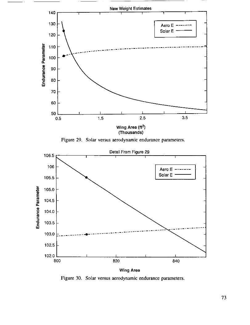
E
D.
G)o¢::
:3"10t,-
IJJ
140
130
120
i 110100
90.m
_ ao
70
60
5O
New Weight Estimates
0.5
I I I I I I
Aero E -Solar E
D
Figure 29.
I I I I I I
106.5
106
105.5
105.0
104.5
104.0
103.5
103.0
102.5
102.0800
1.5 2.5 3.5
Wing Area (ft 2)
(Thousands)
Solar versus aerodynamic endurance parameters.
Detail From Figure 29I I I I
I Aero ESolar E
Figure 30.
I820 840
Wing Area
Solar versus aerodynamic endurance parameters.
?3

W = 1.729 Sw°'778+0.353 Sw+196.52 , (108)
with AR = 15. Table 14 lists the revised aircraft specifications.
Table 14. Final design specifications.
etot[S = 2.165 W/ft 2
WtotlS = 0.976 lb/ft 2
Wtot = 817.54 lb
Wa,, = 24.531b
Waf -= 3101bWpt = 200 lbS = 838 ft
Sw = 616.18 ft 2
St = 221.82 ft 2
bw = 96.14 ft
bt = 57.68 ft
AR= 15
Pprop = 1,467.5 WRe = 351,722V = 91.70 ft/s
Pay - 147.2 W
Ppt = 200 WCL312/CD = 103.2
CL= 1.31
CD = 0.0145
Cw = 6.41 ft
ct = 3.85 ftL/D = 90.34
F. Mission and Aircraft Specifications
It should be noted that the ability to fly year-round indicates that flight during the spring, fall,
and summer months has more freedom of operation. For instance, on September 20 there is approx-
imately twice the solar power available as on December 22. This extra energy can be used to allow
operations at higher latitudes or altitudes, to increase airspeed, or to increase the payload opera-tions. Also, additional energy would be available for corrections in the flight path should relatively
high winds blow the HASPP off course. In order to achieve the lift coefficient given in table 14, which
allows flight under worse case conditions, the HASPP airfoil has an angle of attack of 4 °, which is
due to the built-in angle of incidence.
The San Joaquin Valley covers an area from 35 ° to 40 ° N. latitude and 119 ° to 122 ° W. longi-
tude. During the days of least daylight, the HASPP might need to travel south, to circle at a given
latitude, or to raise the nose to maintain flight dependent on the latitude range of the flight path.
Figures 31 and 32 are illustrations of the increased freedom of operation the HASPP could experi-
ence over a year's time. Figure 31 is a graph of solar and aerodynamic endurance parameters at 36 °
N. latitude for the mission duration. As before, an endurance parameter equality indicates that flightis feasible at the corresponding conditions. Solar endurance parameters less than aerodynamic
endurance parameters imply that there is more than enough energy available to operate at those
conditions. Therefore, on figure 31, conditions above the line for a 10 ° angle of attack' are not con-
sidered possible since the wing will stall at approximately 12°. Figure 32 offers similar information at40 ° N. latitude.
The HASPP configuration is a monoplane with one motor turning two in-line two-bladed pro-
pellers. One propeller will be a tractor type and the other a pusher. They are in-line and along the
longitudinal axis of the airplane so as not to create any asymmetrical thrust problems should one
propeller experience difficulties. The airplane design is a twin-boom tail type, with the oversizedhorizontal stabilizer and two rudders on either side of the tail.
74
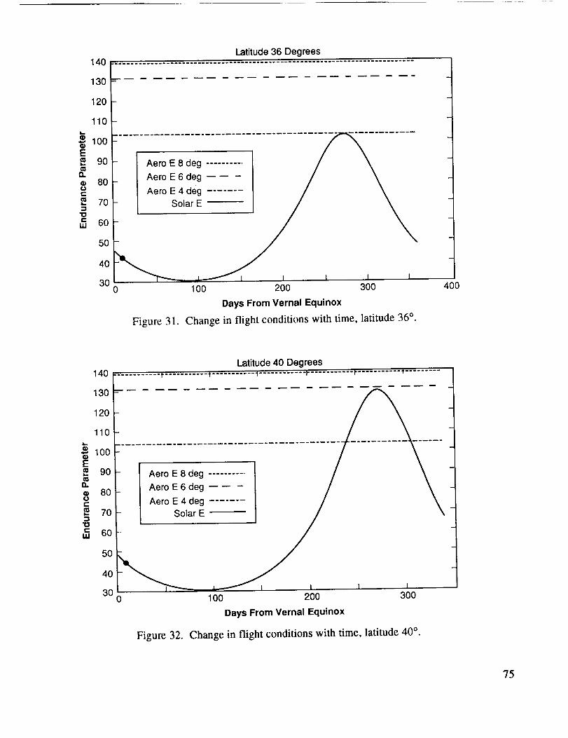
Latitude 36 Degrees
E
o
"1ot-
ILl
130
120
110
100
90
8O
70
60
5O
40
30
m
- Aero E 8 deg .......... / "_
_ Aero E6deg ---- - / \
Aero E 4 deg ....... / \
0 1O0 200 300
Days From Vernal Equinox
Figure 31. Change in flight conditions with time, latitude 36 °.
ii
40O
Em
Or-E
cW
Latitude 40 Degrees140 r ........... t ........... t ........... _............ t-........... t ........... _.........
/130
120
110
100
90
8O
7O
60
5O
40
30
Aero E 8 deg ..........
Aero E 6 deg
Aero E 4 degSolar E
Figure 32.
I I I I100 200 300
Days From Vernal Equinox
Change in flight conditions with time, latitude 40° .
75
Creating a power required curve illustrates the velocities corresponding to certain angles ofattack as well as the associated power settings necessary to obtain this velocity. This curve is cre-ated using equations:
L = (pl2)V2SwCL, (5b)
and:
Dtot = (p 12) V 2[SCo(a)+Spara] (71)
Points on the Pre versus V curve are formed in two steps. The first step is to use equation (5e):
V = [2WI(pSwCL)] u2 (109)
with the substitution of W = L. An angle of attack is assumed and the associated Ct. value is taken
from figure 21, resulting in a velocity from equation (109). The next step is to take the Co value from
figure 21 for the same a and equation (5d) for power required. Equation (71) is substituted intoequation (5d) yielding:
P re = ( p 12 )V3[ SwCD( Ot) +Spara] • (11o)
The velocity in this equation is that derived from equation (109). The parasite area, Spara, refers tothe coefficients of parasite drag for the various airplane parts except the wing as given in equations(25) and (26). Thus, equation (110) becomes:
Pre = (P/2) V3Sw[CDw+ 0.36Cot+O.7536/Sw+O.O003] 1.356/0.7618 . (111)
Figure 33 shows the velocities associated with a range of angles of attack for the data in table 14. At
a level flight attitude and at 36 ° latitude, the HASPP will travel at 27.91 m/s (91.70 ft/s, 54.3 kt, or
62.53 mph). On June 19, the HASPP would have a vertical rate of climb, Vc, of 185.3 ft/min from
equation (54). Stalling speed of the aircraft is approximately 70.9 ft/s. Flying a racetrack course of
radius 4.35 km (14,300 ft), dictated by the sensor scan width, the airplane will travel 288,000 m
(944,000 ft) and begin the 180 ° turn of radius r = 4.35 km (14,000 ft). The angle of bank associatedwith this turn would be calculated from: 38
y = tan -1 (V2/(g r)) (112)
as 1.05 ° at 1 g.
The flight path described above allows for the same area to be covered approximately twice a
day during daylight hours, or four times in a 24-h period. Coverage by sensor scans would be greaterand would encompass an area 169.48 nm (1,030,000 ft) by 9.40 nm (57,000 ft) or 1,250,000 acres
(5.45x101° ft 2) which is 1,900 mi 2. The HASPP will actually fly through 2.70 of latitude and 0.08 ° of
longitude. The design latitude of 36 ° is an average chosen for convenience, the airplane might need tofly nose up during the critical days of winter as it passes through the higher latitudes or it could circleat the lower latitudes until more sunlight was available.
76

1.50
1.40
1.30
g .20n- o
i="oa. 1.10
1.00
I Ias a function of angle of attackI I I I I I I
/1012
0.90 I I I I I I l I
0 20 40 60 80 1 O(
Velocity (ft/s)
Figure 33. Power required curve.
Chapter XIV. CONCLUSIONS
In conclusion, this design study has demonstrated that with current or near current technol-
ogy it is possible to build a HASPP capable of flying a mission for twelve continuous months. The
future aspects of this design include: refinement of the design, vehicle dynamics analysis, control
system design, specification development, definition of launch and recovery procedures, and proto-
type testing.
An agricultural monitoring mission has been presented for a HASPP because of the recog-
nized need for improved crop management techniques. Also, information on agricultural monitoring
needs is readily available. However, as stated previously, a HASPP has the capacity of functioningin a number of roles. In fact, the HASPP designed in this paper iscapable of carrying an additional
132 lb and still maintaining flight year round at 36 ° latitude with a 6 ° angle of attack during the criti-cal winter days. This would, of course, mean higher angles of attack at higher latitudes, but flight
under these conditions is still feasible. The 90-percentile winds at altitude, that the HASFP should
be designed to compensate for, are less than the stalling speed of the aircraft at a 12 ° angle of
attack, therefore, the nose up flight attitude would not be a concern. The potential increase in payload
capacity would allow for additional monitoring of crops (in addition to the capability of performing
nighttime sensing during the months of increased sunlight) or the performance of a dual mission. TheHASPP could carry equipment to detect forest fires or perform some communication service while
providing farmers with needed data.
77
The final result is a useful airplane of reasonable proportions. Previously it was discussed
that $10 million annually would be available for HASPP manufacture and operation, were farmers
willing to pay the same as they pay consultants now. While actual cost figures on the HASPP arenot available, this figure is assumed to be more than sufficient. The initial construction and launch of
the craft would be costly, as well as the acquisition of the ground facility. Beyond this initialization,
the only continuing costs would be the staff necessary to operate the avionics and the down link of
agricultural data. When maintenance on the HASPP is necessary, it would be brought down for
recovering, replacement of damaged solar cells, and general refurbishment of other aircraft systems.
In short, the HASPP is a superior means of crop management at a reduced cost. The HASPP,
as presented in this report or with another mission, is practical and can be a reality. A complete listof the aircraft specifications and a summary cf the design is presented in table 15.
The future aspects of this design include: refinement of the design, vehicle dynamics analysis,control system design, specification development, definition of launch and recovery procedures, and
prototype testing. Following a detailed completion of this design, a cost analysis would be neces-sary.
78
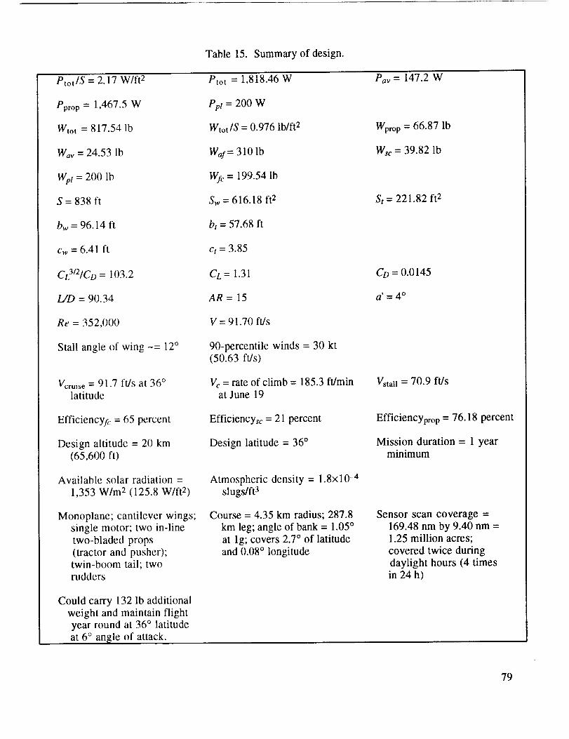
Table 15. Summaryof design.
Ptot/S = 2.17 W/ft 2
Pprop = 1,467.5 W
Wtot = 817.54 lb
Way = 24.53 lb
Wpt = 200 lb
S = 838 ft
bw = 96.14 ft
cw = 6.41 ft
CL3/2[CD = 103.2
L/D = 90.34
Re = 352,000
Stall angle of wing -= 12 °
Vcruise = 91.7 ft/s at 36 °latitude
Efficiencyfc = 65 percent
Design altitude = 20 km(65,600 ft)
Available solar radiation =
1,353 W/m 2 (125.8 W/ft 2)
Monoplane; cantilever wings;
single motor; two in-line
two-bladed props
(tractor and pusher);twin-boom tail; two
rudders
Could carry 132 lb additional
weight and maintain flight
year round at 36 ° latitude
at 6 ° an_le of attack.
etot = 1,818.46 W
pp_ = 200 w
Wtot ]S = 0.976 lb/ft 2
Wa:=3101b
Wfc = 199.54 lb
Sw= 616.18 ft 2
bt = 57.68 ft
ct = 3.85
CL= 1.31
AR= 15
V = 91.70 ft/s
90-percentile winds = 30 kt
(50.63 ft/s)
Vc = rate of climb = 185.3 ft/minat June 19
Efficiencysc = 21 percent
Design latitude = 36 °
Atmospheric density = 1.8×10 -4
slugs/ft 3
Course = 4.35 km radius; 287.8
km leg; angle of bank = 1.05 °
at lg; covers 2.7 ° of latitude
and 0.08 ° longitude
Pav = 147.2 W
Wprop = 66.87 lb
Wsc = 39.82 lb
St = 221.82 ft 2
CD = 0.0145
a' = 4 °
Vstal 1 = 70.9 ft/s
Efficiencyprop = 76.18 percent
Mission duration = 1 yearminimum
Sensor scan coverage =
169.48 nm by 9.40 nm=1.25 million acres;
covered twice during
daylight hours (4 timesin 24 h)
79
REFERENCES
.
.
.
o
*
.
*
8.
o
10.
11.
12.
13.
14.
15.
Youngblood, J.W., and Jackson, R.D.: "Airborne Reconnaissance in the Civilian Sector:
Agriculture Monitoring From High-Altitude Power Platforms." Society of Photo-Optical
Instrumentation Engineers 27th Annual International Technical Symposium, August 21-26,1983.
Henderson, B.W.: "Boeing Condor Raises UAV Performance Levels." Aviation Week and
Space Technology, April 23. 1990.
Kuhner, M.B., Earhart, R.W., Madigan, J.A., and Ruck, E.T.: "Applications of a High Altitude
Powered Platform (HAPP)." NASA CR 158466, September 1977.
Morris, C.E.K.: "Microwave-Powered Unmanned, High-Altitude Airplanes." Journal ofAircraft, vol. 21, No. 12, December 1984.
Graves, E.B.: "The Feasibility of a High-Altitude Aircraft Platform With Consideration of
Technological and Societal Constraints." NASA TM 84508, June 1982, pp. 60-78.
Youngblood, J.W., and Talay, T.A.: "Solar-Powered Airplane Design for Long-Endurance,
High-Altitude Flight.'" AIAA paper 82-0811, 1982.
Stender, W.: "Sailplane Weight Estimation." OSTIV, June 1969.
MacCready, P.B., Lissaman, P.B.S., Morgan, W.R., and Burke, J.D.: "Sun-Powered Aircraft
Design." AIAA paper 81--0916, May 12-14, 1981.
Stansell, J.: "Planes That Fly by the Sun." New Scientist, June 25, 1981.
Boucher, R.J.: "Project Sunrise." AIAA paper 79-1264, June 13, 1979.
Youngblood, J.W., Talay, T.A., and Pegg, R.J.: "Design of Long-Endurance UnmannedAirplanes Incorporating Solar and Fuel Cell Propulsion." AIAA paper 84-1430, June 11-13,1984.
Youngblood, J.W., Darrel, W.L., Johnson, R.W., and Harriss, R.C.: "Airborne Spacecraft--A
Remotely Powered, High Altitude RPV for Environmental Applications." Electronic and
Aerospace Systems Conference, October 9-11, 1979.
Parry, J.F.W.: "A Solar Powered Observation Platform." Defense Advanced Research ProjectsAgency RDA-TR 4300-088, July 1974.
Hall, D.W., Fortenbach, C.D., Dimiceli, E.V., and Parks, R.W.: "A Preliminary Study of SolarPowered Aircraft and Associated Power Trains." NASA CR 36991983, 1983.
Hall, D.W., and Hall, S.A.: "Structural Sizing of a Solar Powered Aircraft." NASA CR 172313,April 1984.
80

16. Jackson,R.D., andYoungblood,J.W.: "Agriculture's Eyein the Sky." Cropsand SoilsMagazine,October 1983.
17. Jackson,R.D.: "RemoteSensingof Vegetation."SPIE,vol. 475,RemoteSensing,1984.
18. Interview with Bill Barnes,GoddardSpaceFlight Center,Greenbelt,MD, August23, 1990.
19. "Solar Cells for PhotovoltaicGenerationof Electricity," 1979.
20. "PhotovoltaicEnergyProgramSummaryFiscalYear 1988,"vol. I andII, SolarEnergyResearchInstitute.
21. Zweibel, K.: "SecondGenerationSolarCells." The World andI, May 1988.
22. Irving, F.G., andMorgan,D.: "The Feasibilityof anAircraft Propelledby Solar Energy." AIAApaper74-1042, September11-13, 1974.
23. Keith, F.: "Principles of SolarEngineering,"1978.
24. Vogt, S.T., and Proeschel,R.A.: "SpaceStationPhotovoltaicPowerModule Design," I989.
25. "Space StationBattery SystemDesignand Development," 1989.
26. Hubbard,H.M.: "Photovoltaics:TodayandTomorrow.'"Science,vol. 244,April 21, 1989.
27. Personalcorrespondencewith Stan Vernon, Spire Corporation.
28. Personal correspondence with Gary Virshup, Varian, Palo Alto, CA, October 18, 1989.
29. Gale, R.P., KOPIN Corporation, Taunton, MA, October 6, 1989, and January 11, 1990.
30. Personal correspondence with Kim W. Mitchell, ARCO Solar, Inc., Camarillo, CA.
31. Green, M.A., University of New South Wales, Kensington, New South Wales, November 9,1989.
32. Wortmann, F.X.: "The Quest for High Lift." AIAA paper 74-1018, September 11-13, 1974.
33. Althaus, D.: "Experimental Results From the Laminar Wind Tunnel of the Institut fur Aero-
und Gasdynamik Der Universitat Stutart." Stultgarter Profilkatalog 1,1972.
34. Ghia, K.N., Osswald, G., and Ghia, U.: "Study of Low-Reynolds Number Separated Flow Past
the Wortmann FX 63-137 Airfoil." Low Reynolds Number Aerodynamics, June 1989.
35. McMasters, J.H., and Palmer, G.M.: "At the Threshold of Man-Powered Flight." Astronautics
& Aeronautics, September 1977.
36. Coming, G.: "Supersonic and Subsonic Airplane Design." Braun-Brumfield, Inc., 1970.
81

37. McCormick, B.W.: "Aerodynamics,Aeronautics,andFlight Mechanics."JohnWiley and Sons,1979.
38. Von Mises,R.: "Theory of Flight." Dover Publications,Inc., New York, 1959.
39. Liebeck,R.G.: "Designof SubsonicAirfoil for High Lift." Journalof Aircraft, September1978.
40. Miley, S.J.:"'Onthe Designof Airfoils for Low ReynoldsNumbers."AIAA paper74-1017,September1974.
41. Karpinski, A.P.: "New Application of Silver-ZincBatteriesfor Orbiting Spacecraft,"1989.
42. Interview with PaulProkopuis,NASA/LeRC,March 1990.
43. Interview and personalcorrespondencewith Tom Maloney,Sverdrup,LeRC, Cleveland,OH,February25, 1991.
44. Bechtel National, Inc., "Handbookfor BatteryEnergyStoragein PhotovoltaicPowerSystems."DOE contract No. DE-AC03-78ET26902,November1979.
45. Haas,R.J., andChawathe,A.K,: "SpaceStationNickel-HydrogenCell DesignandDevelopment," 1989.
46. Interviews with Jeff Brewer,NASA/MSFC,AL, March 1990.
47. Adams, D.R., et al.: "Fuel Cells Powerfor the Future." Fuel Cell ResearchAssociates,1960.
48. Appleby, A.J., and Foulkes,R.R.: "Fuel Cell Handbook."Van NostrandReinhold, 1989.
49. Interview with Roy Lanier, NASA/MSFC,AL, November2, 1989.
50. Curran, P., andFaulkner,D.: "A Samarium-CobaltMotor-Controller for Mini-RPVPropulsion.'"17th IECEC, 1982.
51. Curran,P.D., SundstandCorporation,Rockford,IL, November6, 1989.
52. Spotts, M.F.: "Design of Machine Elements." Prentice-Hall, Inc., 1978.
53. Interview with Cary Spitzer, NASA/LaRC, VA, March 1990.
54. Stragnac, T.W.: "Wind Study for High Altitude Platform Design." NASA RP-1044, December1979.
55. Turner, R.E., and Hill, C.K.: "Terrestrial Environment (Climatic) Criteria Guidelines for Use in
Aerospace Vehicle Development." NASA TM 82473, 1982.
56. USAF Air Research and Development Command, Air Force Research Division, Geophysics
Research Directorate: "Handbook of Geophysics." The MacMillan Co., New York, 1961.
82

57. Interview with William H. Phillips,NASA/LaRC,VA, June8, 1989.
58. Interview andpersonalcorrespondencewith JamesW. Youngblood,NASA/LaRC, VA,October25, 1989.
59. Interview with Tom Nelson,DuPont,November2, 1989.
60. Congiliano, P.E.:"An ExperimentalInvestigationof theLow ReynoldsNumberPerformanceofthe Lissaman7769 Airfoil." AIAA paper83-0647,January1983.
61. "Soaring," vol. 47, No. 11,November1983.
62. Departmentof Energy,SolarEnergyResearchInstitute: "Photovoltaics:Converting Sunlight toElectricity," January1988.
83
APPROVAL
HIGH ALTITUDE SOLAR POWERED PLATFORM
By M.D. Bailey
The information in this report has been reviewed for technical content. Review of any
information concerning Department of Defense or nuclear energy activities or programs has been
made by the MSFC Security Classification Officer. This report, in its entirety, has been determinedto be unclassified.
j.C. BA_ ____
Director, Structures and Dynamics Laboratory
84
"_" U.S. GOVERNMENT PRINTING OFFICE 1992 -- 631--060 160092