
NAVAL
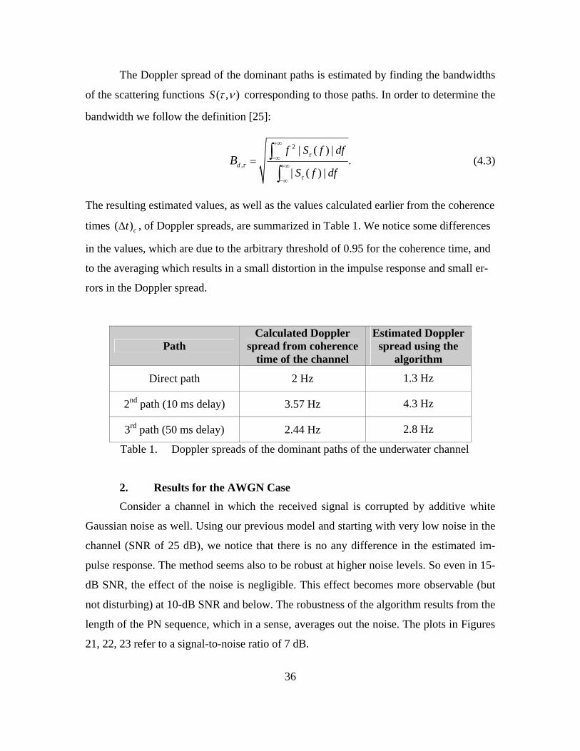
POSTGRADUATE SCHOOL
MONTEREY, CALIFORNIA
THESIS
UNDERSEA ACOUSTIC PROPAGATION CHANNEL ESTIMATION
by
Spyridon Dessalermos
June 2005
Thesis Advisor: Joseph Rice Thesis Co-advisor: Roberto Cristi
Approved for public release, distribution is unlimited

THIS PAGE INTENTIONALLY LEFT BLANK

i
REPORT DOCUMENTATION PAGE Form Approved OMB No. 0704-0188 Public reporting burden for this collection of information is estimated to average 1 hour per response, including the time for reviewing instruction, searching existing data sources, gathering and maintaining the data needed, and completing and reviewing the collection of information. Send comments regarding this burden estimate or any other aspect of this collection of information, including suggestions for reducing this burden, to Washington headquarters Services, Directorate for Information Operations and Reports, 1215 Jefferson Davis Highway, Suite 1204, Arlington, VA 22202-4302, and to the Office of Management and Budget, Paperwork Reduction Project (0704-0188) Washington DC 20503. 1. AGENCY USE ONLY (Leave blank)
2. REPORT DATE June 2005
3. REPORT TYPE AND DATES COVERED Master’s Thesis
4. TITLE AND SUBTITLE: Undersea Acoustic Propagation Channel Estimation 6. AUTHOR(S) Spyridon Dessalermos
5. FUNDING NUMBERS
7. PERFORMING ORGANIZATION NAME(S) AND ADDRESS(ES) Naval Postgraduate School Monterey, CA 93943-5000
8. PERFORMING ORGANIZATION REPORT NUMBER
9. SPONSORING /MONITORING AGENCY NAME(S) AND ADDRESS(ES) N/A
10. SPONSORING/MONITORING AGENCY REPORT
NUMBER 11. SUPPLEMENTARY NOTES The views expressed in this thesis are those of the author and do not reflect the official policy or position of the Department of Defense or the U.S. Government. 12a. DISTRIBUTION / AVAILABILITY STATEMENT Approved for public release, distribution is unlimited
12b. DISTRIBUTION CODE
13. ABSTRACT (maximum 200 words) This research concerns the continuing development of Seaweb underwater networking. In this type of wireless net-
work the radio channel is replaced by an underwater acoustic channel which is strongly dependent on the physical properties of
the ocean medium and its boundaries, the link geometry and the ambient noise. Traditional acoustic communications have in-
volved a priori matching of the signaling parameters (e.g., frequency band, source level, modulation type, coding pulse length)
to the expected characteristics of the channel. To achieve more robust communications among the nodes of the acoustic net-
work, as well as high quality of service, it is necessary to develop a type of adaptive modulation in the acoustic network. Part of
this process involves estimating the channel scattering function in terms of impulse response, the Doppler effects, and the link
margin. That is possible with the use of a known probe signal for analyzing the response of the channel. The estimated channel
scattering function can indicate the optimum signaling parameters for the link (adaptive modulation). This approach is also ef-
fective for time varying channels, including links between mobile nodes, since the channel characteristics can be updated each
time we send a probe signal.
15. NUMBER OF PAGES
142
14. SUBJECT TERMS Adaptive modulation, Underwater Communications, Channel Estimation, Acoustic propagation
16. PRICE CODE
17. SECURITY CLASSIFI-CATION OF REPORT
Unclassified
18. SECURITY CLASSIFICA-TION OF THIS PAGE
Unclassified
19. SECURITY CLAS-SIFICATION OF AB-STRACT
Unclassified
20. LIMITATION OF ABSTRACT
UL NSN 7540-01-280-5500 Standard Form 298 (Rev. 2-89) Prescribed by ANSI Std. 239-18

ii
THIS PAGE INTENTIONALLY LEFT BLANK

iii
Approved for public release, distribution is unlimited
UNDERSEA ACOUSTIC PROPAGATION CHANNEL ESTIMATION
Spyridon Dessalermos Lieutenant Junior Grade, Hellenic Navy
B.S., Hellenic Naval Academy, 1998
Submitted in partial fulfillment of the requirements for the degree of
MASTER OF SCIENCE IN ELECTRICAL ENGINEERING AND
MASTER OF SCIENCE IN APPLIED PHYSICS
from the
NAVAL POSTGRADUATE SCHOOL June 2005
Author: Spyridon Dessalermos
Approved by: Joseph Rice Thesis Advisor
Roberto Cristi Thesis Co-advisor
James Luscombe Chairman, Department of Physics John P. Powers Chairman, Department of Electrical and Computer Engineering

iv
THIS PAGE INTENTIONALLY LEFT BLANK
v
ABSTRACT
This research concerns the continuing development of Seaweb underwater net-
working. In this type of wireless network the radio channel is replaced by an underwater
acoustic channel which is strongly dependent on the physical properties of the ocean me-
dium and its boundaries, the link geometry and the ambient noise. Traditional acoustic
communications have involved a priori matching of the signaling parameters (e.g., fre-
quency band, source level, modulation type, coding pulse length) to the expected charac-
teristics of the channel. To achieve more robust communications among the nodes of the
acoustic network, as well as high quality of service, it is necessary to develop a type of
adaptive modulation in the acoustic network. Part of this process involves estimating the
channel scattering function in terms of impulse response, the Doppler effects, and the link
margin. That is possible with the use of a known probe signal for analyzing the response
of the channel. The estimated channel scattering function can indicate the optimum sig-
naling parameters for the link (adaptive modulation). This approach is also effective for
time varying channels, including links between mobile nodes (e.g. two submarines), since
the channel characteristics can be updated each time we send a probe signal.

vi
THIS PAGE INTENTIONALLY LEFT BLANK
vii
TABLE OF CONTENTS
I. INTRODUCTION........................................................................................................1 A. UNDERWATER ACOUSTIC NETWORKS................................................1 B. ADAPTIVE MODULATION .........................................................................2 C. SCOPE OF THE THESIS...............................................................................3
II. UNDERWATER CHANNEL .....................................................................................5 A. SOUND PROPAGATION IN THE OCEAN ................................................5 B. NOISE ...............................................................................................................8 C. SIGNAL DISTORTION DUE TO MULTIPATH PROPAGATION.........9
1. Energy Time Spread..........................................................................10 2. Doppler Shift - Doppler Spread........................................................11
D. IMPULSE RESPONSE PROFILE - IMPORTANCE ...............................12 E. UNDERWATER CHANNEL CHARACTERISTICS PARAMETERS ..13 F. DIFFERENT TYPES OF FADING CHANNELS......................................14 G. POSSIBLE MODEL OF UNDERWATER CHANNEL............................16 H. CHAPTER SUMMARY................................................................................17
III. CONTEXT OF CHANNEL ESTIMATION ...........................................................19 A. RTS / CTS PROCEDURE ............................................................................19 B. PROBE SIGNALS .........................................................................................20
1. LFM Chirp .........................................................................................20 2. DSSS Signal ........................................................................................21
C. CHANNEL ESTIMATION...........................................................................24 D. CHAPTER SUMMARY................................................................................27
IV. DEVELOPMENT OF METHOD ON ARTIFICIAL CHANNEL .......................29 A. ARTIFICIAL CHANNEL.............................................................................29 B. TRANSMITTED PROBING SIGNAL........................................................32 C. RESULTS OF THE METHOD ....................................................................32
1. Results for the Case Without Noise..................................................32 2. Results for the AWGN Case..............................................................36
D. CHAPTER SUMMARY................................................................................39
V. NEW ENGLAND SHELF CHANNEL ESTIMATION.........................................41 A. DESCRIPTION OF THE NEW ENGLAND SHELF EXPERIMENT....41 B. DESCRIPTION OF THE PROBE SINGAL...............................................44 C. CHANNEL ESTIMATION RESULTS .......................................................46
1. Received Signal at a Distance of 700 Meters ...................................47 2. Received Signal at a Distance of 1100 Meters .................................53 3. Received Signal at a Distance of 1650 Meters .................................57 4. Received Signal at a Distance of 2300 Meters .................................61 5. Received Signal at a Distance of 3050 Meters .................................65 6. Received Signal at a Distance of 3700 Meters .................................69 7. Received Signal at a Distance of 4350 Meters .................................73 8. Received Signal at a Distance of 5000 Meters .................................77

viii
9. Received Signal at a Distance of 5750 Meters .................................81 10. Received Signal at a Distance of 6550 Meters .................................84 11. Summary of the Results.....................................................................88
D. CHAPTER SUMMARY................................................................................89
VI. CONCLUSIONS AND FUTURE WORK...............................................................91 A. CONCLUSIONS ............................................................................................91 B. FUTURE WORK...........................................................................................92
APPENDIX. MATLAB CODES .............................................................................95
LIST OF REFERENCES....................................................................................................117
INITIAL DISTRIBUTION LIST .......................................................................................121

LIST OF FIGURES Figure 1. Seaweb illustration (After Ref. 2.) .....................................................................1 Figure 2. Adaptive modulation Process ............................................................................3 Figure 3. Ray Tracing example, for source depth at 30 meters.........................................6 Figure 4. Absorption in seawater – Solid line is for T 0o= and dashed line for
(After Ref. 9.) ......................................................................................7 T 20o=Figure 5. Tonpilz transducer frequency response (After Ref. 12.)....................................8 Figure 6. Deep water ambient noise (After Ref. 9.) ..........................................................9 Figure 7. Multipath effect on a sinusoidal pulse .............................................................11 Figure 8. Examples of frequency non-selective / selective fading channels...................15 Figure 9. Example of an LFM chirp................................................................................21 Figure 10. Comparison of the autocorrelations of PN sequence and random binary
sequence...........................................................................................................22 Figure 11. Direct Sequence Spread Spectrum Signal Generation.....................................23 Figure 12. Amplitude of the three impulse responses components in absolute time ........30 Figure 13. Multipath intensity profile of artificial signal (in time delay) .........................30 Figure 14. Coherence function of the three components of impulse response..................31 Figure 15. Exact and estimated impulse response for the direct path ...............................33 Figure 16. Exact and estimated impulse response for the 2nd path....................................33 Figure 17. Exact and estimated impulse response for the 3rd path ....................................34 Figure 18. Estimated Multipath intensity profile of artificial signal (in time delay) ........34 Figure 19. Estimated normalized scattering function of the artificial channel .................35 Figure 20. Exact and estimated impulse response for direct path (SN dB).............37 R 7=Figure 21. Exact and estimated impulse response for the 2nd path ( dB) ..........37 SNR 7=Figure 22. Exact and estimated impulse response for the 3rd path (SN dB)............38 R 7=Figure 23. Estimated Multipath intensity profile of artificial signal (AWGN case /
dB)....................................................................................................39 SNR 7=Figure 24. Estimated normalized scattering function of the artificial noisy channel........39 Figure 25. Overview of the Forefront-2 experiment site. The 50 meters isobath is
plotted ..............................................................................................................41 Figure 26. Rough illustration of the experiment ...............................................................42 Figure 27. Transmitter– Receiver positions during the experiment ..................................43 Figure 28. Sound speed profile..........................................................................................44 Figure 29. Transmitted probe waveform...........................................................................44 Figure 30. Spectrograms of the probes..............................................................................46 Figure 31. Received signal at distance 700 meters ...........................................................47 Figure 32. Eigenrays plot for distance 700 meters............................................................48 Figure 33. Estimated impulse response at 700 meters using LFM chirp ..........................49 Figure 34. Estimated impulse response at 700 meters using DSSS signal in bandpass....50 Figure 35. Estimated impulse response at 700 meters using DSSS signal in baseband....50 Figure 36. Multipath Intensity Profile at 700 meters using DSSS signal in baseband......51 Figure 37. Multipath Intensity Profile at 700 meters - Bellhop theoretical estimate ........51 Figure 38. Estimated Scattering function of the channel at distance 700 meters..............52 ix

x
Figure 39. Received signal at distance 1100 meters .........................................................53 Figure 40. Eigenrays plot for distance 1100 meters..........................................................54 Figure 41. Estimated impulse response at 1100 meters using LFM chirp ........................54 Figure 42. Estimated impulse response at 1100 meters using DSSS signal in bandpass..54 Figure 43. Estimated impulse response at 1100 meters using DSSS signal in baseband..55 Figure 44. Multipath Intensity Profile at 1100 meters using DSSS signal in baseband....56 Figure 45. Multipath Intensity Profile at 1100 meters - Bellhop theoretical estimate ......56 Figure 46. Estimated Scattering function of the channel at distance 1100 meters............56 Figure 47. Received signal at distance 1650 meters .........................................................58 Figure 48. Eigenrays plot for distance 1650 meters..........................................................58 Figure 49. Estimated impulse response at 1650 meters using LFM chirp ........................59 Figure 50. Estimated impulse response at 1650 meters using DSSS signal in bandpass..59 Figure 51. Estimated impulse response at 1650 meters using DSSS signal in baseband..59 Figure 52. Multipath Intensity Profile at 1650 meters using DSSS signal in baseband....60 Figure 53. Multipath Intensity Profile at 1650 meters - Bellhop theoretical estimate ......60 Figure 54. Estimated Scattering function of the channel at distance 1650 meters............61 Figure 55. Received signal at distance 2300 meters .........................................................62 Figure 56. Eigenrays plot for distance 2300 meters..........................................................62 Figure 57. Estimated impulse response at 2300 meters using LFM chirp ........................63 Figure 58. Estimated impulse response at 2300 meters using DSSS signal in bandpass..63 Figure 59. Estimated impulse response at 2300 meters using DSSS signal in baseband..63 Figure 60. Multipath Intensity Profile at 2300 meters using DSSS signal in baseband....64 Figure 61. Multipath Intensity Profile at 2300 meters - Bellhop theoretical estimate ......64 Figure 62. Estimated Scattering function of the channel at distance 2300 meters............65 Figure 63. Received signal at distance 3050 meters .........................................................66 Figure 64. Eigenrays plot for distance 3050 meters..........................................................66 Figure 65. Estimated impulse response at 3050 meters using LFM chirp ........................67 Figure 66. Estimated impulse response at 3050 meters using DSSS signal in bandpass..67 Figure 67. Estimated impulse response at 3050 meters using DSSS signal in baseband..67 Figure 68. Multipath Intensity Profile at 3050 meters using DSSS signal in baseband....68 Figure 69. Multipath Intensity Profile at 3050 meters - Bellhop theoretical estimate ......68 Figure 70. Estimated Scattering function of the channel at distance 3050 meters............69 Figure 71. Received signal at distance 3700 meters .........................................................70 Figure 72. Eigenrays plot for distance 3700 meters..........................................................70 Figure 73. Estimated impulse response at 3700 meters using LFM chirp ........................71 Figure 74. Estimated impulse response at 3700 meters using DSSS signal in bandpass..71 Figure 75. Estimated impulse response at 3700 meters using DSSS signal in baseband..71 Figure 76. Multipath Intensity Profile at 3700 meters using DSSS signal in baseband....72 Figure 77. Multipath Intensity Profile at 3700 meters - Bellhop theoretical estimate ......72 Figure 78. Estimated Scattering function of the channel at distance 3700 meters............73 Figure 79. Received signal at distance 4350 meters .........................................................74 Figure 80. Eigenrays plot for distance 4350 meters..........................................................74 Figure 81. Estimated impulse response at 4350 meters using LFM chirp ........................75 Figure 82. Estimated impulse response at 4350 meters using DSSS signal in bandpass..75 Figure 83. Estimated impulse response at 4350 meters using DSSS signal in baseband..75

xi
Figure 84. Multipath Intensity Profile at 4350 meters using DSSS signal in baseband....76 Figure 85. Multipath Intensity Profile at 4350 meters - Bellhop theoretical estimate ......76 Figure 86. Estimated Scattering function of the channel at distance 4350 meters............77 Figure 87. Received signal at distance 5000 meters .........................................................78 Figure 88. Eigenrays plot for distance 5000 meters..........................................................78 Figure 89. Estimated impulse response at 5000 meters using LFM chirp ........................79 Figure 90. Estimated impulse response at 5000 meters using DSSS signal in bandpass..79 Figure 91. Estimated impulse response at 5000 meters using DSSS signal in baseband..79 Figure 92. Multipath Intensity Profile at 5000 meters using DSSS signal in baseband....80 Figure 93. Multipath Intensity Profile at 5000 meters - Bellhop theoretical estimate ......80 Figure 94. Estimated Scattering function of the channel at distance 5000 meters............81 Figure 95. Received signal at distance 5750 meters .........................................................82 Figure 96. Estimated impulse response at 5750 meters using LFM chirp ........................82 Figure 97. Estimated impulse response at 5750 meters using DSSS signal in bandpass..82 Figure 98. Estimated impulse response at 5750 meters using DSSS signal in baseband..83 Figure 99. Multipath Intensity Profile at 5750 meters using DSSS signal in baseband....83 Figure 100. Estimated Scattering function of the channel at distance 5750 meters............84 Figure 101. Received signal at distance 5650 meters .........................................................85 Figure 102. Estimated impulse response at 6550 meters using LFM chirp ........................85 Figure 103. Estimated impulse response at 6550 meters using DSSS signal in bandpass..86 Figure 104. Estimated impulse response at 6550 meters using DSSS signal in baseband..86 Figure 105. Multipath Intensity Profile at 6550 meters using DSSS signal in baseband....87 Figure 106. Estimated Scattering function of the channel at distance 6550 meters............87 Figure 107. Summarization of the MIPs for the 10 different cases ....................................88 Figure 108. Summarization of the Scattering functions for the 10 different cases .............89

xii
THIS PAGE INTENTIONALLY LEFT BLANK
xiii
LIST OF TABLES Table 1. Doppler spreads of the dominant paths of the underwater channel .................36 Table 2. Doppler spreads of the dominant paths of the noisy underwater channel .......38 Table 3. Summary of the 10 cases .................................................................................47 Table 4. Doppler spreads and shifts of the dominant paths at distance of 700 meters ..53 Table 5. Doppler spreads and shifts of the dominant paths for distance of 1100
meters...............................................................................................................57 Table 6. Doppler spreads and shifts of the dominant paths for distance of 1650
meters...............................................................................................................61 Table 7. Doppler spreads and shifts of the dominant paths for distance of 2300
meters...............................................................................................................65 Table 8. Doppler spreads and shifts of the dominant paths for distance of 3050
meters...............................................................................................................69 Table 9. Doppler spreads and shifts of the dominant paths for distance of 3700
meters...............................................................................................................73 Table 10. Doppler spreads and shifts of the dominant paths for distance of 4350
meters...............................................................................................................77 Table 11. Doppler spreads and shifts of the dominant paths for distance of 5000
meters...............................................................................................................81 Table 12. Doppler spreads and shifts of the dominant paths for distance of 5750
meters...............................................................................................................84 Table 13. Doppler spreads and shifts of the dominant paths for distance of 6550
meters...............................................................................................................88

xiv
THIS PAGE INTENTIONALLY LEFT BLANK

xv
ACKNOWLEDGMENTS
First and foremost, I must acknowledge the constant and unconditional support I
received from my advisors, Joseph Rice and Roberto Cristi. Their explanations and guid-
ance led me to the completion of this thesis. I would like to express my appreciation to
Mike Porter and Paul Hursky for providing me the data of the SignalEx-B experiment. I
also wish to thank Paul Baxley for deriving the Bellhop numerical model’s plots for the
eigenrays and the Multipath Intensity Profiles of the eight cases.
I also wish to dedicate this thesis to my thoughtful and supportive father and
brothers, and especially to the sweet memory of my mother. I would like also to express
my sincere appreciation to my Taiwanese friend Wan-Chun for her help and support, as
well as to my Greek, American and International colleagues here at NPS for their friend-
ship.

xvi
THIS PAGE INTENTIONALLY LEFT BLANK

xvii
EXECUTIVE SUMMARY
Seaweb is an organized network of battery-operated acoustic modem nodes de-
ployed on the seabed. Those nodes support bidirectional communications between them,
as well as with a gateway node. Seaweb is designed to provide command and control to
Unmanned Underwater Vehicles (UUVs) from shore facilities or surface ships, provide
communications between submerged submarines and land bases, and enable wide area
undersea surveillance in littoral waters.
During the last decade numerous experiments took place in many different acous-
tic channels. One very interesting result from those experiments is that communication
performance exhibits time-varying characteristics strongly dependent on the variability of
the underwater channels themselves. In this thesis we analyze the characteristics and pa-
rameters of the underwater channel that causes the communication between two nodes to
be so environment dependent.
In Chapter II, we describe how the sound propagates in the sea and consider the
colored ambient noise existing in the acoustic medium. We analyze how a signal passing
through this underwater channel is distorted both in the time and frequency domains. We
investigate the importance of the impulse response, develop the characteristic parameters
of the channel and use a theoretical model to describe it.
In Chapter III, we describe the Request to send / Clear to send and shake protocol
which precedes communication in Seaweb. We explain how we can incorporate a probe
signal, which is a known signal of special format, for purposes of obtaining the channel
parameters. We analyze what characteristics a signal needs in order to be used as a probe
signal, and then refer to the most usual ones. We describe an efficient method that en-
ables estimation of the scattering function of the channel. This method uses a Direct Se-
quence spread spectrum signal as a probe signal.
In Chapter IV, we develop an artificial channel with known characteristics. By
passing a DSSS signal in baseband through this channel, we implement the previously

xviii
mentioned method to the received signal to get back the scattering function of the chan-
nel. The scattering function explains by itself every aspect of the channel. We also exam-
ine how the addition of white Gaussian noise influences the accuracy of the estimation.
In Chapter V, we analyze data from a Seaweb experiment (New England Shelf
experiment – 17-20 April 2000). After a general description of the experiment and of the
various probe signals sent, we estimate the characteristics of the real underwater channel
using various methods, including the one we described previously. We can compare then
the results received from each different method. The data were recorded in ten different
ranges, so the channel estimation takes place ten times. It is also very interesting to ob-
serve the way in which the signal is affected by the channel in gradually increased dis-
tances. Some useful conclusions are derived.

I. INTRODUCTION
A. UNDERWATER ACOUSTIC NETWORKS Over the last decade, the U.S. Navy has begun developing underwater acoustic
networks [1,2]. Those networks need to be designed to provide command and control to
Unmanned Underwater Vehicles (UUVs) from shore facilities or surface ships, support
communications between submerged submarines and land bases, and enable wide area
undersea surveillance in littoral waters. The product of this development is Seaweb. Sea-
web is an organized network of battery-operated acoustic modem nodes deployed on the
seabed (Figure 1). Those nodes support bidirectional communications between them, as
well as with gateway nodes. The nodes are networked to allow the hopping of data from a
source node to a destination node through a combination of other intermediate nodes.
During the last decade numerous experiments took place in many different acoustic
channels [3]. One very interesting aspect of those experiments is that communication per-
formance exhibits variability related to the variability of the underwater channels them-
selves. On those experiments a network of nodes cover wide areas (such as a five by fif-
teen nautical miles area) exchanging data between them.
Figure 1. Seaweb illustration (After Ref. 2.)
1
B. ADAPTIVE MODULATION The modem presently used in Seaweb is the Benthos modem employing a modu-
lation scheme involving non-coherently processed frequency shift keying (FSK) [2,4].
The performance of any other modulation scheme has to be compared with the perform-
ance of non-coherent FSK, since it provides robust communications and relatively high
data rates. The performance of phase coherent signaling degrades more rapidly under se-
vere channel distortion whereas the non-coherent FSK is much more robust [5,6]. In the
current implementation of Seaweb, the parameters of the communication link such as
frequency band of operation, modulation scheme, modem output power, and error correc-
tion coding type are determined prior to deployment. The a priori choice of signaling pa-
rameters tends to be overly conservative and non-optimal. The variability of the acoustic
channel suggests that a more appropriate way to deal with those communication parame-
ters is to determine dynamically which combination of those will give us the optimum
communication scheme. This means that the signaling parameters can change for each
exchange of data between two nodes, depending on the existing characteristics of the
channel. As a result, the link would use the communication scheme with the highest pos-
sible data rate and the minimum possible probability of error (probably on the order of
). In the same view, the link would use the most appropriate frequency band and
transmit the minimum required amount of power. The literature refers to this technique as
adaptive modulation [7,8]. The proposed scheme of adaptive modulation process for
Seaweb is presented in Figure 2. The parts highlighted with yellow are analyzed in this
thesis.
510−
2

3
Figure 2. Adaptive modulation Process
C. SCOPE OF THE THESIS
A smart modem is a modem that, after receiving some known probe signal of a
special format, will determine the characteristics of the channel, such as impulse re-
sponse, Doppler shift, and signal-to-noise ratio. Based on the estimated channel condi-
tions, it selects the communication parameters. The goal of this thesis was to provide an
understanding of underwater channel estimation for determining the characteristics if the
channel. The thesis is organized as follows.
In Chapter II, we investigate the underwater channel. We examine the factors that
make this channel so interesting but difficult for acoustic communications. We compare
the underwater channel with the traditional radio channel for cellular communications, to
improve our understanding.
In Chapter III, we examine the method of channel estimation. We describe a prac-
tical mechanism for obtaining the channel characteristics in the acoustic modem. We con-
sider the theory of channel estimation.
In Chapter IV we create an artificial channel with known characteristics and pass
a probe signal through this channel. Then, by processing the received signal, we obtain
RE
CE
IVE
R
TR
AN
SMIT
TE
R
Demodulate RTS Reconstruct transmitted Request To Send Transmission. waveform
Clear To Send Estimate channel scattering function+Parameters
DATA TRANSFER
Determine h(τ,t) / Doppler / SNR
Map channel characteristics against available repertoires and signal techniques
Specify comms parameters in CTS
Final decision

4
characteristics of the artificial channel. This artificial channel is a test channel, useful for
confirming our implementation of the channel estimation algorithm.
In Chapter V, we process data from an actual experiment (New England Shelf ex-
periment – 17-20 April 2000). Using the code developed in Chapter IV, we determine the
characteristics of the channel. We describe the conditions of this experiment, the format
of the data used and also refer in the problems encountered in extracting the scattering
function from the set of real data.
Chapter VI presents a summary with conclusions and goals achieved. Finally, we
discuss the goal of adaptive modulation.
In the Appendix the Matlab codes used to generate the plots for the simulated and
the real channel, are presented.

II. UNDERWATER CHANNEL
This chapter analyzes the basic characteristics of the underwater channel. Starting
from basic acoustics and ray propagation, we move on to the acoustic communication
channel and discuss the signal distortion effects in time and in the frequency domain. We
also define the various types of fading channels, and illustrate the most usual mathemati-
cal models describing their behavior. Then we define the impulse response and demon-
strate how it influences the received signal.
A. SOUND PROPAGATION IN THE OCEAN The ocean is an acoustic waveguide limited above by the sea surface and below
by the seafloor. The sea surface can be modeled as a pressure release boundary and the
sea floor as a second fluid medium (Pekeris Waveguide) [9]. The result is no loss of
acoustic energy to air, but almost always a loss of energy to the second medium. The de-
gree of this effect depends on the characteristics of the bottom (sound speed – density)
and on the incident angle of the acoustic wave to the bottom. So each time the acoustic
wave impinges the bottom, it suffers a loss in strength.
The propagation of sound in the ocean can be described in various ways, but for
our purposes in this thesis, we follow ray theory, an approach borrowed from optics. This
theory is based on the assumption that energy travels along reasonably well defined paths
through the medium. However, rays are not exact representations of waves, but only ap-
proximations that are valid under certain rather restrictive conditions [10]. The ocean wa-
ter column is not a homogeneous medium and the sound speed varies significantly as
function of depth. So the acoustic “rays” in the ocean refract according to Snell’s law.
Snell’s law provides a simple formula for calculating the ray declination angle at any
depth z based only on the declination angle at any other depth and knowledge of the
sound speed:
( ) ( )( ) ( ) ( )( )cos cosoc z z c z zθ = oθ (2.1)
where is the sound speed at depth z. A general rule for ray propagation is that a ray
always bends toward the neighboring region of lower sound speed. If we know the sound
( )c z
5
speed profile of the water column, we can model the sound propagation in this environ-
ment.
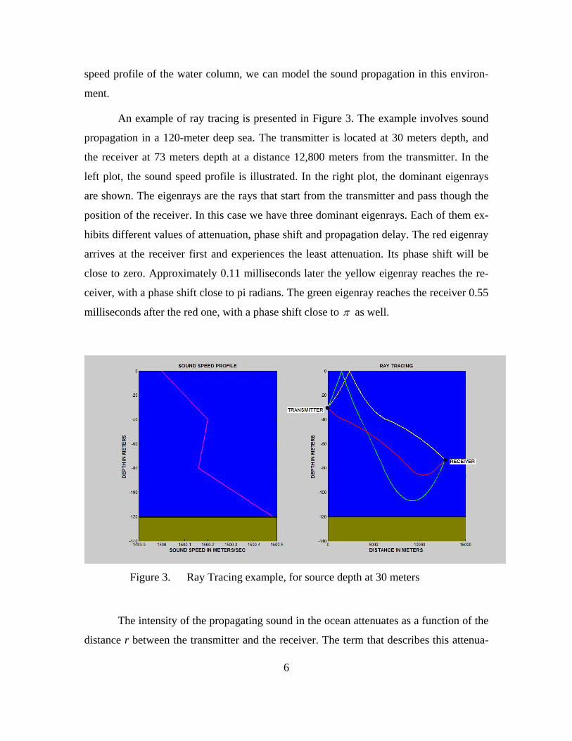
An example of ray tracing is presented in Figure 3. The example involves sound
propagation in a 120-meter deep sea. The transmitter is located at 30 meters depth, and
the receiver at 73 meters depth at a distance 12,800 meters from the transmitter. In the
left plot, the sound speed profile is illustrated. In the right plot, the dominant eigenrays
are shown. The eigenrays are the rays that start from the transmitter and pass though the
position of the receiver. In this case we have three dominant eigenrays. Each of them ex-
hibits different values of attenuation, phase shift and propagation delay. The red eigenray
arrives at the receiver first and experiences the least attenuation. Its phase shift will be
close to zero. Approximately 0.11 milliseconds later the yellow eigenray reaches the re-
ceiver, with a phase shift close to pi radians. The green eigenray reaches the receiver 0.55
milliseconds after the red one, with a phase shift close to π as well.
Figure 3. Ray Tracing example, for source depth at 30 meters
The intensity of the propagating sound in the ocean attenuates as a function of the
distance r between the transmitter and the receiver. The term that describes this attenua-
6

tion is the transmission loss (TL). It is determined by combining the signal loss from
source to receiver due to a combination of geometric spreading and sound absorption.
Geometric spreading from the transmitter is in the form of spherical spreading up
to a range equal to the water depth of the channel. Spherical spreading loss is propor-
tional to 21 r . Beyond this range, cylindrical spreading approximates the propagation.
Cylindrical spreading loss is proportional to 1 r . [11]
The absorption of sound in seawater depends on numerous parameters such as,
temperature, salinity, depth, pH, frequency. A general rule is that as frequency increases
the absorption of sound in the ocean is stronger. Figure 4 illustrates the absorption coeffi-
cient as a function of frequency for 0oT = C and C, for a depth of 0 m, pH20oT = 8=
and ppt (parts per thousand). [9] 35S =
Figure 4. Absorption in seawater – Solid line is for 0oT = and dashed line for
(After Ref. 9.)
20oT =
7

The spectral bandwidth of an acoustic communication link has restrictions on its
size. Those restrictions have two origins. With higher acoustic frequencies the absorption
increases (see Figure 4) and the effective distance of the communication link will be very
limited, so we have a restriction on the upper side of the band. The second problem is the
non-uniform frequency response of underwater sound projectors. We would like to have
a relatively flat frequency response along a wide frequency band. This is usually hopeless
because of the way those transducers are built. At typical communications frequencies
between 15 and 30 kHz, they can have a relatively flat response along a bandwidth of 15
kHz, at best. An example of a typical frequency non-uniform response of a Tonpilz trans-
ducer with a matching layer is shown in Figure 5 [12].
Figure 5. Tonpilz transducer frequency response (After Ref. 12.)
B. NOISE
The ambient noise of the ocean is not Gaussian and colored. Below 500 Hz the
major contribution to ambient noise is from distant shipping and biological noise. From
500 Hz to 50 kHz the local sea surface is the strongest source. This is actually the fre-
8

quency band of interest, since most acoustic modems operate in this band. As a result, the
channel noise varies depending on the conditions (sea state, wind), as illustrated in Figure
6. Above 50 kHz the ocean turbulence and the thermal agitation of the water molecules
are the predominant noise source. [13]
Figure 6. Deep water ambient noise (After Ref. 9.)
Traditionally the theory of communications assumes Additive White Gaussian
Noise (AWGN). However AWGN is not representative of the acoustic channel. The
noise is neither white nor Gaussian. The result is that communications performance is
worst and also the analysis is much more complicated.
C. SIGNAL DISTORTION DUE TO MULTIPATH PROPAGATION In the case of underwater acoustic communications, the signal is carried by acous-
tic pressure waves. In this channel there are some interesting effects taking place, which
put severe limitations in the communications. The first effect is illustrated in Figure 3.
We see that, for the geometry shown, the acoustic waves reach the receiver following
9

10
three different paths. Destructive interference by the multipath propagation structure cre-
ates severe fading in the channel [14, 15].
Fading is caused by interference of two or more replicas of the transmitted signal
arriving at the receiver at slightly different times following different paths. These differ-
ent components are called multipaths. They combine at the receiver to give a resultant
signal, which can vary widely in amplitude and phase, depending on the distribution of
the intensity and relative propagation time of the waves and the bandwidth of the trans-
mitted signal. The multipath signal viewed in the frequency domain, exhibites different
spectral components of the signal being affected differently by the channel. In other
words the frequency response of the channel is not flat over the bandwidth of the signal.
Another important characteristic of the multipath propagation is the time variation
in the structure of the acoustic medium (waves, wind, current) and the motion of either
the receiver or the transmitter. As a result, the signal passing through the underwater
channel is distorted both in the time and frequency domains.
1. Energy Time Spread Consider the simplified case of Figure 3. We assume a sinusoidal signal with a
transmit duration of one millisecond. The acoustic wave (following Figure 3) follows
three different paths. Each path has some attenuation, some phase shift and some propa-
gation delay. The transmitted pulse is illustrated on the left side of Figure 7 and the re-
ceived pulse on the right side. As we can see, the received pulse is distorted and its en-
ergy is spread in time.
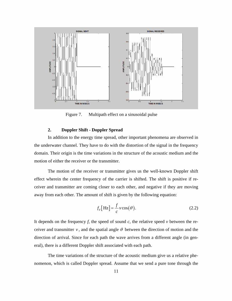
Figure 7. Multipath effect on a sinusoidal pulse
2. Doppler Shift - Doppler Spread In addition to the energy time spread, other important phenomena are observed in
the underwater channel. They have to do with the distortion of the signal in the frequency
domain. Their origin is the time variations in the structure of the acoustic medium and the
motion of either the receiver or the transmitter.
The motion of the receiver or transmitter gives us the well-known Doppler shift
effect wherein the center frequency of the carrier is shifted. The shift is positive if re-
ceiver and transmitter are coming closer to each other, and negative if they are moving
away from each other. The amount of shift is given by the following equation:
[ ] ( )Hz cos .dff vc
θ= (2.2)
It depends on the frequency f, the speed of sound c, the relative speed v between the re-
ceiver and transmitter v , and the spatial angle θ between the direction of motion and the
direction of arrival. Since for each path the wave arrives from a different angle (in gen-
eral), there is a different Doppler shift associated with each path.
The time variations of the structure of the acoustic medium give us a relative phe-
nomenon, which is called Doppler spread. Assume that we send a pure tone through the
11
channel. If the channel is time invariant, we do not notice any spectral broadening in the
received tone. However, time variations of a channel result in a broadening of the spectral
line. This effect is what we call Doppler spread. The Doppler spread, just like the Dop-
pler shift, has a different value for each path. [16]
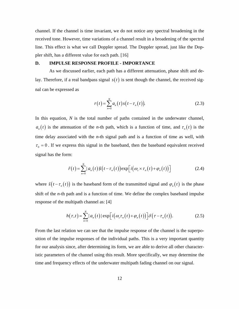
D. IMPULSE RESPONSE PROFILE - IMPORTANCE As we discussed earlier, each path has a different attenuation, phase shift and de-
lay. Therefore, if a real bandpass signal ( )s t is sent though the channel, the received sig-
nal can be expressed as
(2.3) ( ) ( ) ( )(0
.N
n nn
r t a t s t tτ=
= −∑ )
In this equation, N is the total number of paths contained in the underwater channel,
is the attenuation of the n-th path, which is a function of time, and is the
time delay associated with the n-th signal path and is a function of time as well, with
( )na t ( )n tτ
0 0τ = . If we express this signal in the baseband, then the baseband equivalent received
signal has the form:
( ) ( ) ( )( ) ( ) ( )(0| | exp
N
n n c n nn
r t a t s t t i t tτ ω τ ϕ=
)⎡ ⎤= − × +⎣ ⎦∑% % (2.4)
where is the baseband form of the transmitted signal and is the phase
shift of the n-th path and is a function of time. We define the complex baseband impulse
response of the multipath channel as: [4]
( )( ns t tτ−% )
).nτ τ−
( )n tϕ
(2.5) ( ) ( ) ( ) ( )( ) ( )(0
, | | expN
n c n nn
h t a t i t t tτ ω τ ϕ δ=
⎡ ⎤= +⎣ ⎦∑
From the last relation we can see that the impulse response of the channel is the superpo-
sition of the impulse responses of the individual paths. This is a very important quantity
for our analysis since, after determining its form, we are able to derive all other character-
istic parameters of the channel using this result. More specifically, we may determine the
time and frequency effects of the underwater multipath fading channel on our signal.
12

E. UNDERWATER CHANNEL CHARACTERISTICS PARAMETERS The underwater channel can be characterized by at least two parameters. The first
characterizes the time variations and the other the frequency variations of the channel.
The Fourier transform of the impulse response ( ),h tτ with respect to the time de-
lay, is given by the relation
(2.6) ( ) ( ) 2, , i ftH f t h t e dtπτ+∞
−
−∞
= ∫ .
The autocorrelation of the channel impulse response Fourier transform (with respect to
time delay), is given by the relation
1 1 1 11( , ; , ) { ( , ) ( , )},2HS f f t t H f t H f t= Ε (2.7)
where stand for the expected value of the function inside the brackets. { }E
If we take the inverse Fourier transform of ( )1; ,HS f t t∆ with respect to f∆ , we obtain
( ) ( ) (21 1; , ; , .i f
h HP t t S f t t e d fπττ+∞ ∆
−∞)= ∆∫ ∆ (2.8)
When the channel is wide sense stationary in the t variable, ( ) (1; , ,h hP t t P tτ τ= ∆ ) where
. In the case when , 1t t t∆ = − 0t∆ = ( )hP τ is the average power out of the channel as a
function of the time delay τ . It is called the power delay profile or multipath intensity
profile [Ref. 4, 16]. The range of τ over which the power delay profile is nonzero is the
multipath spread of the channel. The multipath spread is the first of the two important
parameters and describes the time dispersive nature of the channel. Some typical values
of the multipath spread for an underwater channel are 10-20 ms, compared to the cellular
wireless communication channel, where they are 1-10 µs [3, 4]. The greater the multipath
spread, the more dispersive the channel will be.
mT
Now consider . In the case when ( ;HS f t∆ ∆ ) 0t∆ = , ( )HS f∆ is the frequency
correlation function. The range of f∆ over which the frequency correlation function is
13
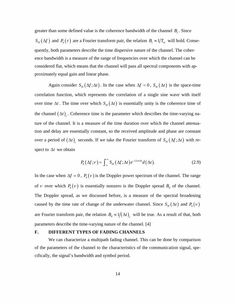
greater than some defined value is the coherence bandwidth of the channel cB . Since
and (HS f∆ ) ( )hP τ are a Fourier transform pair, the relation 1c mB T≈ will hold. Conse-
quently, both parameters describe the time dispersive nature of the channel. The coher-
ence bandwidth is a measure of the range of frequencies over which the channel can be
considered flat, which means that the channel will pass all spectral components with ap-
proximately equal gain and linear phase.
Again consider . In the case when ( ;HS f t∆ ∆ ) 0f∆ = , ( )HS t∆ is the space-time
correlation function, which represents the correlation of a single sine wave with itself
over time . The time over which t∆ ( )HS t∆ is essentially unity is the coherence time of
the channel ( . Coherence time is the parameter which describes the time-varying na-
ture of the channel. It is a measure of the time duration over which the channel attenua-
tion and delay are essentially constant, so the received amplitude and phase are constant
over a period of ( seconds. If we take the Fourier transform of with re-
spect to we obtain
)ct∆
)ct∆ ( ;HS f t∆ ∆ )
).
t∆
(2.9) ( ) ( ) (2; ; i th HP f S f t e d tπνν
+∞ − ∆
−∞∆ = ∆ ∆ ∆∫
In the case when , 0f∆ = ( )hP ν is the Doppler power spectrum of the channel. The range
of ν over which ( )hP ν is essentially nonzero is the Doppler spread dB of the channel.
The Doppler spread, as we discussed before, is a measure of the spectral broadening
caused by the time rate of change of the underwater channel. Since and ( )HS t∆ ( )hP ν
are Fourier transform pair, the relation ( )1d cB t≈ ∆ will be true. As a result of that, both
parameters describe the time-varying nature of the channel. [4]
F. DIFFERENT TYPES OF FADING CHANNELS
We can characterize a multipath fading channel. This can be done by comparison
of the parameters of the channel to the characteristics of the communication signal, spe-
cifically, the signal’s bandwidth and symbol period.
14

Time dispersion due to multipath causes the transmitted signal to experience ei-
ther flat or frequency selective fading. If the channel has a constant gain and linear phase
response over a bandwidth which is greater than the bandwidth of the transmitted signal
(i.e., cB is large in comparison with the BW), the channel is said to be frequency-
nonselective or flat fading. In the time domain this means that all of the multipath com-
ponents arrive within the symbol duration. On the other hand, if cB is small in compari-
son with the BW, significant distortion of the signal occurs and the channel is said to be
frequency-selective. In this case successive pulses interfere with each other.
Figure 8 illustrates the concept of flat and frequency selective fading.
Figure 8. Examples of frequency non-selective / selective fading channels
Depending on how rapidly the transmitted signal changes as compared to the rate
of change of the channel, a channel may be classified either as a fast fading or slow fad-
ing channel. If the symbol duration is smaller than the coherence time, then the received
amplitude and phase are effectively constant for the duration of at least one symbol and
15
the channel is said to be slowly fading. But if the received amplitude and phase fluctuate
over time periods that are short compared to the duration of a symbol, the channel is said
to be fast fading.
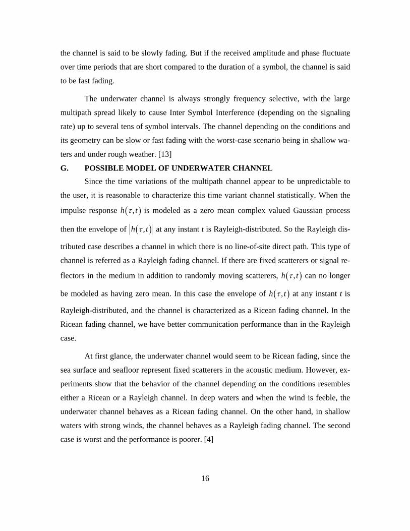
The underwater channel is always strongly frequency selective, with the large
multipath spread likely to cause Inter Symbol Interference (depending on the signaling
rate) up to several tens of symbol intervals. The channel depending on the conditions and
its geometry can be slow or fast fading with the worst-case scenario being in shallow wa-
ters and under rough weather. [13]
G. POSSIBLE MODEL OF UNDERWATER CHANNEL
16
)
Since the time variations of the multipath channel appear to be unpredictable to
the user, it is reasonable to characterize this time variant channel statistically. When the
impulse response ( ,h tτ is modeled as a zero mean complex valued Gaussian process
then the envelope of ( ),h tτ at any instant t is Rayleigh-distributed. So the Rayleigh dis-
tributed case describes a channel in which there is no line-of-site direct path. This type of
channel is referred as a Rayleigh fading channel. If there are fixed scatterers or signal re-
flectors in the medium in addition to randomly moving scatterers, ( ),h tτ can no longer
be modeled as having zero mean. In this case the envelope of ( ),h tτ at any instant t is
Rayleigh-distributed, and the channel is characterized as a Ricean fading channel. In the
Ricean fading channel, we have better communication performance than in the Rayleigh
case.
At first glance, the underwater channel would seem to be Ricean fading, since the
sea surface and seafloor represent fixed scatterers in the acoustic medium. However, ex-
periments show that the behavior of the channel depending on the conditions resembles
either a Ricean or a Rayleigh channel. In deep waters and when the wind is feeble, the
underwater channel behaves as a Ricean fading channel. On the other hand, in shallow
waters with strong winds, the channel behaves as a Rayleigh fading channel. The second
case is worst and the performance is poorer. [4]

17
H. CHAPTER SUMMARY In this chapter, we analyzed the underwater channel and all its characteristics that
make it so interesting and difficult for acoustic communications. Next, we examine the
method of channel estimation by describing a practical mechanism for obtaining the
channel characteristics in the acoustic modem.

18
THIS PAGE INTENTIONALLY LEFT BLANK
19
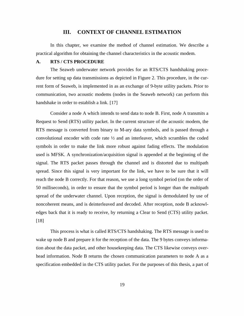
III. CONTEXT OF CHANNEL ESTIMATION
In this chapter, we examine the method of channel estimation. We describe a
practical algorithm for obtaining the channel characteristics in the acoustic modem.
A. RTS / CTS PROCEDURE The Seaweb underwater network provides for an RTS/CTS handshaking proce-
dure for setting up data transmissions as depicted in Figure 2. This procedure, in the cur-
rent form of Seaweb, is implemented in as an exchange of 9-byte utility packets. Prior to
communication, two acoustic modems (nodes in the Seaweb network) can perform this
handshake in order to establish a link. [17]
Consider a node A which intends to send data to node B. First, node A transmits a
Request to Send (RTS) utility packet. In the current structure of the acoustic modem, the
RTS message is converted from binary to M-ary data symbols, and is passed through a
convolutional encoder with code rate ½ and an interleaver, which scrambles the coded
symbols in order to make the link more robust against fading effects. The modulation
used is MFSK. A synchronization/acquisition signal is appended at the beginning of the
signal. The RTS packet passes through the channel and is distorted due to multipath
spread. Since this signal is very important for the link, we have to be sure that it will
reach the node B correctly. For that reason, we use a long symbol period (on the order of
50 milliseconds), in order to ensure that the symbol period is longer than the multipath
spread of the underwater channel. Upon reception, the signal is demodulated by use of
noncoherent means, and is deinterleaved and decoded. After reception, node B acknowl-
edges back that it is ready to receive, by returning a Clear to Send (CTS) utility packet.
[18]
This process is what is called RTS/CTS handshaking. The RTS message is used to
wake up node B and prepare it for the reception of the data. The 9 bytes conveys informa-
tion about the data packet, and other housekeeping data. The CTS likewise conveys over-
head information. Node B returns the chosen communication parameters to node A as a
specification embedded in the CTS utility packet. For the purposes of this thesis, a part of

the RTS signal is used for channel estimation at node B. In the future, the channel esti-
mate is the input information to the acoustic modem for determining the optimal commu-
nication parameters.
B. PROBE SIGNALS
In order to determine the channel characteristics, node A must send node B a sig-
nal known to B. This signal is referred to as a probe signal and must have a special for-
mat. The probe signal passess through the underwater channel and it is distorted in time
and frequency as seen in Chapter II. Since node B knows in advance what the form of the
probe is, it can determine what the effect of the channel was by the use of appropriate
signal processing.
As discussed earlier, the RTS signal is very important in Seaweb, so the informa-
tion carried during the RTS procedure has to reach the target node without errors. Node B
demodulates the RTS signal, and reconstructs a clean replica of the waveform transmitted
by node A. This waveform, or an appended special-purpose waveform, serves as the
channel probe.
The probe signal must be suitable to estimate the dynamics of the underwater
channel. Wideband probe signals provide high resolution in time and frequency and they
are often used in practical systems to measure the channel characteristics. Typical wide-
band signals for this purpose can be a Linear Frequency Modulated (LFM) chirp or a
pseudorandom-noise-spread signal (such as a Direct Sequence Spread Spectrum signal -
DSSS).
1. LFM Chirp The first type of wideband signal that can be used as a probe to the channel is the
Linear Frequency Modulated (LFM) chirp, a sinusoidal signal with frequency sweeping
with time in a linear way. The LFM chirp signal has quadratic phase. The form of an
LFM chirp is
( ) ( )2cos .x t A t tα β γ= + + (3.1)
Its instantaneous frequency is ( ) 2f t tα β= + . We can see that the frequency changes
linearly with time. As a result for our case, the overall signal is wideband. Both the fre- 20

quency band and resolution depend on the values of the time duration of the LFM chirp
and on the parameter α. In the example of LFM chirp shown in Figure 9, the parameters
are set so that the sweeping frequency is in the range 100 to 400 Hz and the chirp dura-
tion is one second. [19]
Figure 9. Example of an LFM chirp
2. DSSS Signal
The second type of signal that can be used for channel sounding is the direct se-
quence spread spectrum (DSSS) signal. This type of signal is obtained by mixing a car-
rier signal with a pseudonoise (PN) random sequence.
The characteristics of the PN sequence have to be like those of a true random bi-
nary sequence. The most important figure of merit for the PN sequence is the autocorrela-
tion function. It has to resemble that of a true random binary sequence. The comparison
of the two autocorrelation functions, as presented in Figure 10, shows great similarity,
except for the periodicity. Also, the greater the number of chips N in the PN sequences,
the better. A PN sequence can be generated by the use of an n-stage shift register where
the output of each stage are properly connected or not connected to an exclusive-or gate
21

whose output is fed back to the input of the shift register. The resulting sequence is called
a maximal-length sequence or just a m-sequence. In a set of length-N m-sequences, some
will have better crosscorrelation properties and those are called preferred m-sequences.
Combining appropriate sets of those, we can get another set of PN sequences which are
called Gold sequences. [Ref. 4]
Figure 10. Comparison of the autocorrelations of PN sequence
and random binary sequence
22
The generation of a DSSS bandpass signal (in the time domain) is now briefly ex-
plained following Figure 11. Assume that we want to transmit three da 1, 0 and 1. We
transform the binary data in the polar binary wave (1 and 1− ) as shown in the first quar-
ter of the figure. The duration of the bit is 0.75 milliseconds, which corresponds to a
bandpass null-to-null bandwidth of 2.67 kHz. In the second part of the figure is an m-
sequence with a length of 15 chips. It is important to notice that 15 chips occupy a time
duration of 0.75 milliseconds (i.e., the duration of one data bit). In order to create the
baseband DSSS signal we multiply the two binary waveforms shown in the first half of
the figure; the resulting signal is shown on the third line. After mixing the baseband

waveform with a carrier of 160 kHz, we get the DSSS/BPSK form which is shown in the
last quarter of the figure. Since the chip duration is 0.05 milliseconds, which is 15 times
smaller than the bit duration, the null-to-null bandwidth of the resulting DSSS/BPSK sig-
nal is 15 times larger than that of an unspread BPSK signal, equal to 20 kHz. In this ex-
ample the length of the spreading code is relatively small, since in practice we use much
longer PN sequences. For acoustic communications, Gold codes of length 2047 are some-
times used.
Figure 11. Direct Sequence Spread Spectrum Signal Generation
In order to demodulate the DSSS/BPSK waveform it first has to be despread. The
receiver’s knowledge about the chipping signal is necessary. If we know the chipping se
23
quence, the spread signal is multiplied with the aligned and synchronized PN sequence
and the resulting waveform is the BPSK signal that is easily demodulated by a conven-
tional BPSK receiver. [20]
Spread spectrum signals have some very important benefits. They are very effi-
cient at suppressing both multi-user interference and channel-induced intersymbol inter-
ference (ISI) due to multipath arrivals. They can also be used for hiding a low-power sig-
nal below the noise floor. This is important because the detection of a DSSS signal by an
unauthorized listener is very difficult. That is the reason DSSS systems are referred to as
Low Probability of Detection (LPD) communications systems. Even if this signal is de-
tected, the knowledge of the PN code is necessary in order to demodulate it. As a result
DSSS systems are referred as Low Probability of Intercept (LPI) communications sys-
tems. For the above mentioned reasons, the implementation of spread spectrum in Sea-
web is desirable. [21]
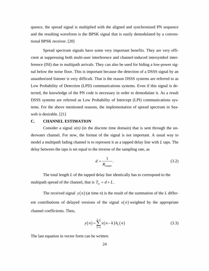
C. CHANNEL ESTIMATION Consider a signal x(n) (in the discrete time domain) that is sent through the un-
derwater channel. For now, the format of the signal is not important. A usual way to
model a multipath fading channel is to represent it as a tapped delay line with L taps. The
delay between the taps is set equal to the inverse of the sampling rate, as
1 .sample
dR
= (3.2)
The total length L of the tapped delay line identically has to correspond to the
multipath spread of the channel, that is mT d L= × .
The received signal (at time n) is the result of the summation of the L differ-
ent contributions of delayed versions of the signal
( )y n
( )x n weighted by the appropriate
channel coefficients. Then,
(3.3) ( ) ( ) ( )1
0
L
kk
y n x n k h n−
=
= −∑
The last equation in vector form can be written:
24

( ) ( ) ( )y n h n x n= (3.4)
where
( )
( )( )
( )
1
1
x n
x nx n
x n L
⎛ ⎞⎜ ⎟
−⎜= ⎜⎜ ⎟⎜ ⎟− −⎝ ⎠
M
⎟⎟ (3.5)
and
( ) ( ) ( ) ( )( )0 1 1 .Lh n h n h n h n−= L (3.6)
The function is the impulse response of the channel, which we introduced
in Chapter II. This function can be written in polar form as
( )kh n
( ) ( ) ( )kj nk kn nh a e θ= where
represents the amplitude and ( )ka n ( )k nθ the phase shift of the underwater channel im-
pulse response at time n and time delay . kd
The method of channel estimation we are going to use in this work uses a DSSS
wideband signal in the input signal ( )x n . In the baseband, this signal has the form
( ) ( ) ( ) ( )( )1 2x n d n p n jp n= + , where 1 and 2p p are two different PN Gold sequences of
the same length, modulated by the same data bit ( )( )d n . The period of the PN sequence
has to be longer than the multipath spread of the channel. Also the chip duration has to be
such that it will give us a signal Bandwidth 2 chipBW T= , much larger than the coherence
bandwidth cB [Ref. 22]. The resulting minimum time resolution in determining the im-
pulse response of the channel will be seconds. In this case the received signal will be
given by
chipT
(3.7) ( ) ( ) ( ) ( ) ( )(1
1 20
.L
kk
r n h n d n p n k jp n k−
=
= − +∑ )−
25

The receiver correlates the received signal with the known spreading sequence delayed
by , and this process is repeated L times for each time delay from 0 to ( sec-
onds. The discrete time between transmitted and received sequences can be computed as:
kd )1 L d−
( ) ( ) ( ) ( )( ) ( )
( ) ( )( ) ( )( ) (
( ) ( ) ( )
1 2
1 2
1
1 2 2
0
1
0
1,2
1 , { }2
, ,
n N
i nN
i
N
i
i m jp i m
i m p i m
c m n r i p d i mL
h m n L p L i mL
h m n i m h m n
δ
δ
+ −
=
−
=
−
=
− − −
= − −
=
= −
)+ −
=−
∑
∑
∑
(3.8)
where ( )tδ is the discrete time impulse.
This shows that, at least in the ideal case, the impulse response of the channel can
be computed by crosscorrelating the transmitted and the received sequences. The assump-
tions are that the two sequences, ( ) ( )1 2n and np p , have ideal autocorrelations and that
there is no noise in the receiver. In practice the result will be deteriorated due to the noise
and the non-ideal correlation properties of the Gold sequence. [22]
Using the previously mentioned method we get an estimate of the impulse re-
sponse of the channel . It is a function of two variables, the time delay m and
the absolute time n . By processing this function we measure the characteristics of the
underwater channel.
( ,esth m n)
The first function we obtain is the multipath intensity profile of the channel, given
by the relation
( ) ( ) 2
1
|1 , |2
N
nh mP h
N =
= ∑ m n (3.9)
where represents the average power output of the channel as a function of time de-
lay. The width of this function is the multipath spread of the channel. As discussed in
Chapter II the coherence bandwidth of the channel is the inverse of the multipath spread
( )hP m
1c mB T= .
26

The second function is the Doppler power spectrum of the channel, which is the
Fourier transform of the spaced-time correlation function of the channel
( ) ( ){h HP Sν = ∆F }n
)
(3.10)
where is defined in Chapter II. It is used to examine the Doppler effects of the
channel, the Doppler spread and the Doppler shift. The Doppler power spectrum
(HS n∆
( )hP ν
is centered in the frequency spectrum in the frequency that corresponds to Doppler shift
and its bandwidth corresponds to the Doppler spread of the underwater channel. As we
examined before, the coherence time of the channel is the inverse of the Doppler spread,
( ) 1 dct B∆ = .
The most useful function is the third one, which combines information about the
frequency and time spread of the channel. It is called the scattering function of the chan-
nel. We can get the scattering function by taking the Fourier transform with respect
to , of the autocorrelation function of the estimated impulse response n∆
( ) ( ), { ,n hS m m nν φ∆= F }∆ , (3.11)
where
( ) ( ) ( )*
0
1, { , ,N
h est estn
m n h m n h m n nN
φ=
∆ = + ∆∑ }.
)
(3.12)
This is a very important function since the knowledge of ( ,S m ν by itself is
enough to give us all the characteristics of the channel (Doppler shift, Doppler spread,
and multipath spread). [23]
D. CHAPTER SUMMARY
In this chapter, we developed our method of channel estimation. In the next two
chapters we implement this method, and apply it first to an artificial channel (Chapter IV)
and then to the data of a real ocean experiment (Chapter V).
27

28
THIS PAGE INTENTIONALLY LEFT BLANK

IV. DEVELOPMENT OF METHOD ON ARTIFICIAL CHANNEL
The first objective in the development and testing of channel estimation is the ap-
plication of the method on an artificial time-varying channel with known characteristics.
The scope of this simulation is to confirm that the channel estimation algorithm works
properly.
A. ARTIFICIAL CHANNEL The received signal can be represented as we developed in the Chapter III by the
superposition of the L delayed replicas of the transmitted signal,
(4.1) ( ) ( ) ( )1
0
L
kk
y t x t k h tτ−
=
= − ∆∑
where ( )x t is the wideband transmitted signal and ( )kh t is the k-th impulse response
component at time t. The artificial channel is constructed according to the structure of
Figure 3, in which we have three discrete paths for the eigenrays. In this representation
the transmitter and receiver are stationary, which implies that there is no Doppler shift
due to relative motion. Environmental parameters such as the roughness of the sea or the
currents in the water column produce a time-varying underwater channel. Each path has a
different time-varying nature and hence a different (nonzero) Doppler spread. The first
path is the direct path, which we assume to have zero time delay and the smallest Doppler
spread. The second and third dominant paths correspond to the surface-reflected eigen-
rays, having constant time delay 10 and 50 milliseconds, respectively, with different
time-varying weights. The amplitudes of the three components of the impulse response
are illustrated in Figure 12 as a function of absolute time. As indicated in this figure,
there is a substantial time variation in their amplitudes in a relatively small period of time
(about 4 seconds). The average multipath intensity profile of the artificial channel as a
function of the time delay is illustrated in Figure 13; clearly, the multipath spread of
the artificial channel is 50 milliseconds.
mT
29

Figure 12. Amplitude of the three impulse responses components in absolute time
Figure 13. Multipath intensity profile of artificial signal (in time delay)
30

In order to assess the resulting Doppler spread of the estimated channel, we de-
velop the space-time correlation function of the known artificial channel, which we intro-
duced in Chapter II. We express this as the autocorrelation of each component of the im-
pulse response
( ) ( ) ( )( ) ( )
2
2
*
*
| } 1,2,3...
| }{|
{|k
k
khk
kk
h t h t tS t
h t h t=
Ε +∆∆ =
Ε (4.2)
In our case, the impulse response has only three nonzero components, so we get three
autocorelation functions, which are illustrated in Figure 14. As we discussed earlier, the
period of time over which this function is approximately constant is the coherence time of
the specific path. Let us consider that the coherence time corresponds to the period t∆
over which is greater than 0.95. The resulting coherence time for the direct path
case is 0.5 seconds, for the second path is 0.28 seconds and for the third path is 0.41 sec-
onds. Since the Doppler spread
( )hkS t∆
dB is equal to the inverse of the coherence time, the cor-
responding spreads for the three paths are 2 Hz, 3.57 Hz and 2.44 Hz, respectively.
Figure 14. Coherence function of the three components of impulse response
31
32
B. TRANSMITTED PROBING SIGNAL The transmitted signal is a Direct Sequence Spread Spectrum (DSSS) baseband
signal like the one studied in Chapter III. It uses PN sequences defined by two different
Gold codes of length 2047, one on the in-phase and the other on the quadrature compo-
nent, modulating the same data bit. These codes are taken from work done by [24] and
the actual sequences were downloaded directly from the web site. The chipping rate used
in the simulation is 4000 chips/second. Each set of 2047 chips represents one bit, so the
data rate of the simulation will be about 2 bps.
The length of the Gold sequence is a very important parameter in our analysis. As
it gets smaller the estimation of the channel characteristics obviously degrades. On the
other hand, as it gets larger, the estimation of the channel is more robust but, since the re-
sult of the method is the average of the impulse response over the length of the PN se-
quence, it gets less accurate, so there is a tradeoff there. From our experiments, it seems
that the choice of length 2047 is a reasonable compromise. In what follows, we send an
information sequence of 8 bits, so the duration of the entire information sequence is 4.094
seconds. In the first case we study an ideal noise-free case. In the second case, the signal
is corrupted by the presence of additive white Gaussian noise (AWGN).
C. RESULTS OF THE METHOD In the following simulation the channel parameters are estimated without noise,
and later with additive white Gaussian noise in the channel.
1. Results for the Case Without Noise
In the upper half of Figure 15 the exact form of the impulse response of the direct
path is shown, whereas in the lower half is the algorithm’s estimate for the same function.
Clearly, we do not get the exact value of the impulse response, but an average estimate of
the next 2047 values of the impulse response, which cover a period of about half a sec-
ond. As a result of that, it seems that the estimate has a time offset of 250 milliseconds
from the actual one. The same happens with the other two components of h(t), corre-
sponding to time delays 10 and 50 milliseconds, that are illustrated in Figures 16 and 17,
respectively. Except for the fact that they are averages and not exact values, the estimates

in all three cases are quite accurate, which means that until this stage the method seems to
be accurate.
Figure 15. Exact and estimated impulse response for the direct path
Figure 16. Exact and estimated impulse response for the 2nd path
33

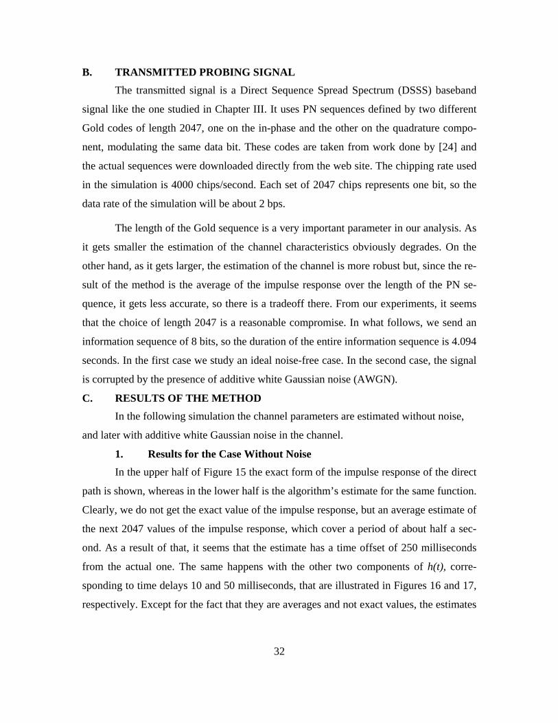
Figure 17. Exact and estimated impulse response for the 3rd path
The resulting multipath intensity profile of the underwater channel is illustrated in
Figure 18. The result is impressive since the estimate multipath intensity profile (MIP) is
almost the same as the original MIP illustrated in Figure 13.
Figure 18. Estimated Multipath intensity profile of artificial signal (in time delay)
34

The most significant function is the scattering function ( , )S τ ν of the channel
which we analyzed in Chapter III. We recall that it combines information about both the
frequency and time spread of the channel. In Figure 19 the normalized scattering function
of the channel is illustrated. Just by inspection of the plot, we can conclude the following:
• The channel has three dominant paths with time delays 0, 10 and 50 milli-
seconds respectively.
• It seems that the second path is stronger than the other two, but this is not
true. The apparent discrepancy is because we took out the DC (zero Dop-
pler) component of the impulse response before processing. We did that for
presentation reasons, so that the Doppler spread would be more obvious.
• The Doppler spread of the second path is by far the largest, the next larger is
the third path and the smaller Doppler spread corresponds to the direct path.
• The Doppler shift of the underwater channel is zero, since the functions are
centered around the zero frequency, consistent with a fixed transmitter-
receiver geometry.
Figure 19. Estimated normalized scattering function of the artificial channel
35
The Doppler spread of the dominant paths is estimated by finding the bandwidths
of the scattering functions ( , )S τ ν corresponding to those paths. In order to determine the
bandwidth we follow the definition [25]:
2
,
| ( ) |.
| ( ) |d
f S f df
S f dfB τ
τ
τ
+∞
−∞+∞
−∞
= ∫∫
(4.3)
The resulting estimated values, as well as the values calculated earlier from the coherence
times ( , of Doppler spreads, are summarized in Table 1. We notice some differences
in the values, which are due to the arbitrary threshold of 0.95 for the coherence time, and
to the averaging which results in a small distortion in the impulse response and small er-
rors in the Doppler spread.
)ct∆
Path Calculated Doppler
spread from coherence time of the channel
Estimated Doppler spread using the
algorithm
Direct path 2 Hz 1.3 Hz
2nd path (10 ms delay) 3.57 Hz 4.3 Hz
3rd path (50 ms delay) 2.44 Hz 2.8 Hz
Table 1. Doppler spreads of the dominant paths of the underwater channel
2. Results for the AWGN Case
Consider a channel in which the received signal is corrupted by additive white
Gaussian noise as well. Using our previous model and starting with very low noise in the
channel (SNR of 25 dB), we notice that there is no any difference in the estimated im-
pulse response. The method seems also to be robust at higher noise levels. So even in 15-
dB SNR, the effect of the noise is negligible. This effect becomes more observable (but
not disturbing) at 10-dB SNR and below. The robustness of the algorithm results from the
length of the PN sequence, which in a sense, averages out the noise. The plots in Figures
21, 22, 23 refer to a signal-to-noise ratio of 7 dB.
36

Figure 20. Exact and estimated impulse response for direct path (SN dB) R 7=
Figure 21. Exact and estimated impulse response for the 2nd path (SN dB) R 7=
37
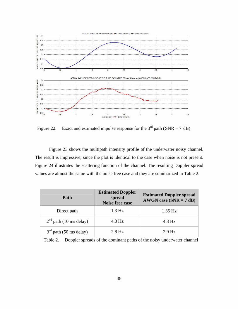
Figure 22. Exact and estimated impulse response for the 3rd path ( dB) SNR 7=
Figure 23 shows the multipath intensity profile of the underwater noisy channel.
The result is impressive, since the plot is identical to the case when noise is not present.
Figure 24 illustrates the scattering function of the channel. The resulting Doppler spread
values are almost the same with the noise free case and they are summarized in Table 2.
Path Estimated Doppler
spread Noise free case
Estimated Doppler spread AWGN case (SNR = 7 dB)
Direct path 1.3 Hz 1.35 Hz
2nd path (10 ms delay) 4.3 Hz 4.3 Hz
3rd path (50 ms delay) 2.8 Hz 2.9 Hz
Table 2. Doppler spreads of the dominant paths of the noisy underwater channel
38
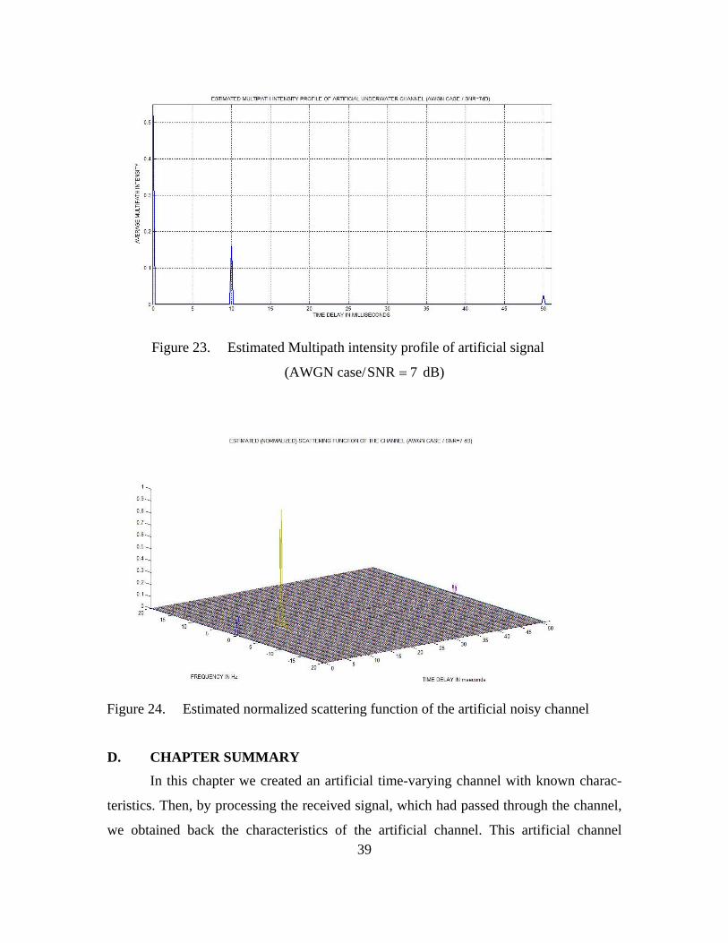
Figure 23. Estimated Multipath intensity profile of artificial signal
(AWGN case/SNR 7= dB)
Figure 24. Estimated normalized scattering function of the artificial noisy channel
D. CHAPTER SUMMARY
In this chapter we created an artificial time-varying channel with known charac-
teristics. Then, by processing the received signal, which had passed through the channel,
we obtained back the characteristics of the artificial channel. This artificial channel 39

40
worked as a test channel to verify that the method works efficiently. In the next chapter,
we process data from an actual experiment (New England Shelf experiment – 17-20 April
2000). Using the same code, we determine the characteristics of the channel. We describe
the conditions of this experiment, the format of the data used and also refer in the prob-
lems encountered in extracting the scattering function from the set of real data.
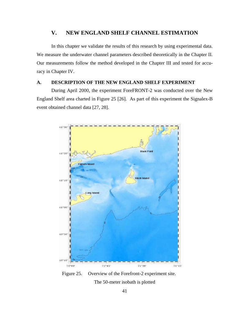
V. NEW ENGLAND SHELF CHANNEL ESTIMATION
In this chapter we validate the results of this research by using experimental data.
We measure the underwater channel parameters described theoretically in the Chapter II.
Our measurements follow the method developed in the Chapter III and tested for accu-
racy in Chapter IV.
A. DESCRIPTION OF THE NEW ENGLAND SHELF EXPERIMENT During April 2000, the experiment ForeFRONT-2 was conducted over the New
England Shelf area charted in Figure 25 [26]. As part of this experiment the Signalex-B
event obtained channel data [27, 28].
Figure 25. Overview of the Forefront-2 experiment site.
The 50-meter isobath is plotted
41
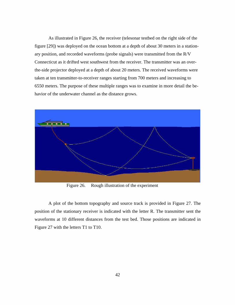
As illustrated in Figure 26, the receiver (telesonar testbed on the right side of the
figure [29]) was deployed on the ocean bottom at a depth of about 30 meters in a station-
ary position, and recorded waveforms (probe signals) were transmitted from the R/V
Connecticut as it drifted west southwest from the receiver. The transmitter was an over-
the-side projector deployed at a depth of about 20 meters. The received waveforms were
taken at ten transmitter-to-receiver ranges starting from 700 meters and increasing to
6550 meters. The purpose of these multiple ranges was to examine in more detail the be-
havior of the underwater channel as the distance grows.
Figure 26. Rough illustration of the experiment
A plot of the bottom topography and source track is provided in Figure 27. The
position of the stationary receiver is indicated with the letter R. The transmitter sent the
waveforms at 10 different distances from the test bed. Those positions are indicated in
Figure 27 with the letters T1 to T10.
42

Figure 27. Transmitter– Receiver positions during the experiment
In order to determine the sound speed profile in the underwater channel, we used
measurements from a CTD instrument, where CTD stands for Conductivity, Temperature
and Depth. The measurement took place at time 20:00, whereas the waveforms were re-
ceived from 21:40 until 02:10, so there is a great possibility that the sound speed profile
changed slightly during this period of time. All the eigenrays estimation plots and the
theoretical impulse response results are based on this measured sound speed profile,
which is illustrated in Figure 28.
43

Figure 28. Sound speed profile
B. DESCRIPTION OF THE PROBE SINGAL During the experiment, the transmitter generated a special type of waveform. The
waveform sent is shown in Figure 29 and consists of different types of probes [30, 31].
The total duration of the test probes was about 2 minutes and 5 seconds. The analytic de-
scription of the various probes follows.
Figure 29. Transmitted probe waveform
44
The first probe consists of 40 LFM chirps with duration of 50 milliseconds each,
with 200 milliseconds silence separating adjacent chips for a total duration of 10 seconds.
Each chirp sweeps through frequencies from 8 to 16 kHz. As we will see later, this type
of probe is useful in determining the impulse response accurately, but it does not yield a
good measurement of the scattering function (specifically Doppler spread) of the channel.
After one second of silence, the second probe is sent. It is a comb of 17 tones of 20 sec-
onds duration. The 17 tones have 500 Hz of separation; the lowest is positioned at 8 kHz
and the highest at 16 kHz. They are useful in measuring the Doppler shift of the underwa-
ter channel. However, the scattering function cannot be derived because as we discussed
earlier, each path has its own Doppler shift, so the result we get from the tone combina-
tion is just a rough estimate of the average Doppler shift.
The next two probe waveforms were not used in the channel estimation in this
work. In both cases, m-sequences are transmitted. In the first case, ten m-sequences are
sent, with and silent gaps in between them are sent. In the second case, ten m-
sequences with are sent but with no silent gaps in between them. The chip rate is
4000 chips/second and the center frequency is 12 kHz. The next probe, which also was
not studied in this work, follows after a silence gap of 1.5 second. It is a music clip band-
shifted to a center frequency of 12 kHz. The next probe is the one we are most interested
in. It has almost the same format with the DSSS signal we discussed in Chapter IV. This
signal is a bandpass direct-sequence spread spectrum signal with center frequency of 12
kHz, a chip rate of 2000 chips/second and a sampling rate of 48000 samples/second. Four
hundred information bits were transmitted. We used two different Gold sequences for
spreading sequences; a different PN sequence is used for the in-phase and quadrature
data, although the same information bit is modulated by each component. Following Fig-
ure 29, we notice that we send six different DSSS probes. The six different probes corre-
spond to six different bit rates of 10, 20, 50, 100, 200 and 400 bps. In all cases, we keep
the chip rate and length of Gold sequence constant. This means that, for example, in the
first case about 400 chips are modulated by one data bit, in the second case 200 chips are
modulated by one data bit, etc. Intuitively, this implementation would result in greater
correlation noise than the ideal case we considered in Chapter IV in which the entire
6m =
10m =
45

length of the Gold sequence was modulated by one data bit. In order to minimize this
problem, we use the lower bit rate probe (first probe with 10 bps) and for the channel es-
timation, we will use a portion of the Gold code and not the entire sequence. In Figure 30,
the most significant probes are summarized by illustrating their frequency spectra.
Figure 30. Spectrograms of the probes
C. CHANNEL ESTIMATION RESULTS We now present the results of the channel estimation method for ten different
ranges and geometries. The first reception was at time 2143 and distance 700 meters.
Subsequent receptions occur every 30 minutes at increasing ranges until the last one at
time 0213 and at a distance of 6550 meters. The ten cases are summarized in Table 3.
46

CASE TIME RANGE (meters) SNR (dB) 1 21:43 700 37 2 22:13 1100 35 3 22:43 1650 31 4 23:13 2300 30 5 23:43 3050 29.5 6 00:13 3700 25 7 00:43 4350 25 8 01:13 5000 16 9 01:43 5700 13 10 02:13 6550 7
Table 3. Summary of the 10 cases
1. Received Signal at a Distance of 700 Meters The signal received at time 2143 and at a distance of 700 meters is plotted in Fig-
ure 31. At this distance, the signal is very strong and the resulting approximate signal-to-
noise ratio is 37 dB. The estimation of the signal-to-noise ratio is done by determining
first the noise power level (during a time period when the signal is not present), and then
the signal plus noise power level, during the time period when the DSSS signal is on. By
processing those two values, we determine the SNR using the relation:
( )S N NSNRN
+ −= (5.1)
Figure 31. Received signal at distance of 700 meters
47

In Figure 32 the eigenrays characterizing the propagation channel are traced using
a numerical model called Bellhop [32]. It is interesting to notice that the first two arrivals
are almost simultaneous. The other 6 eigenrays come into the receiver in pairs, and this is
due to the proximity of the receiver to the seabed.
Figure 32. Eigenrays plot for distance of 700 meters
We first estimate the impulse response of the channel by applying a matched filter
to the probe pulses (using the known 50 milliseconds LFM chirp as the correlation ker-
nel). This method produces accurate measurements of the channel impulse response at
the pulse repetition rate (i.e, 4 measurements/second). The results for the distance of 700
meters are shown in Figure 33. We next use the DSSS signal in the bandpass, following
the method we discussed in Chapters III and IV. The results are shown in Figure 34. Fi-
nally, we determine the impulse response of the channel using the DSSS in the baseband.
This method involves the complicated process of shifting the waveform from bandpass to
baseband. The result is shown in Figure 35. The last two methods give us a measurement
rate of about 24 Hz.
48
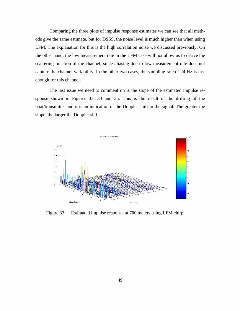
Comparing the three plots of impulse response estimates we can see that all meth-
ods give the same estimate, but for DSSS, the noise level is much higher than when using
LFM. The explanation for this is the high correlation noise we discussed previously. On
the other hand, the low measurement rate in the LFM case will not allow us to derive the
scattering function of the channel, since aliasing due to low measurement rate does not
capture the channel variability. In the other two cases, the sampling rate of 24 Hz is fast
enough for this channel.
The last issue we need to comment on is the slope of the estimated impulse re-
sponse shown in Figures 33, 34 and 35. This is the result of the drifting of the
boat/transmitter and it is an indication of the Doppler shift in the signal. The greater the
slope, the larger the Doppler shift.
Figure 33. Estimated impulse response at 700 meters using LFM chirp
49

Figure 34. Estimated impulse response at 700 meters using DSSS signal in bandpass
Figure 35. Estimated impulse response at 700 meters using DSSS signal in baseband
Using the DSSS signal at baseband, we now derive the average multipath inten-
sity profile of the channel. A preliminary step is to align the impulses to compensate for
motion. There are many techniques to do this, but the one we used is probably the most
accurate and fastest. Starting from the first estimate, we find the first highest peak; then
we look in the next sample to find the highest peak searching only in the neighborhood of
the peak of the previous sample. The method worked precisely for all cases. The multi-
path intensity profile ( )hP τ was analyzed in Chapter II. The resulting multipath intesity
profile for a distance of 700 meters is illustrated in Figure 36. From this figure, we can
determine the multipath spread of the channel which is about 18 milliseconds. The Bell- 50

hop numerical method estimate of the MIP is presented in Figure 37. Note that our Bell-
hop channel modeling neglects boundary losses and shows arrivals with artificially high
intensity. The matching of the measurement with the theoretical results is satisfactory in
terms of multipath arrival structure.
Figure 36. Multipath Intensity Profile at 700 meters using DSSS signal in baseband
Figure 37. Multipath Intensity Profile at 700 meters - Bellhop theoretical estimate
Following the method of Chapter III using the DSSS signal in baseband, we de-
termine the scattering function of the underwater channel (shown in Figure 38) for a dis-
tance of 700 meters. The impressive and expected result is that from a noisy impulse re-
sponse, we get an unambiguous scattering function plot. Clearly, there is a negative Dop-
pler shift consistent with the opening range of the source-receiver geometry and a Dop-
pler spread different for each path. Following Figure 36, we can see that there are nine
dominant paths (those with magnitude greater than 5% of the magnitude of the stronger 51
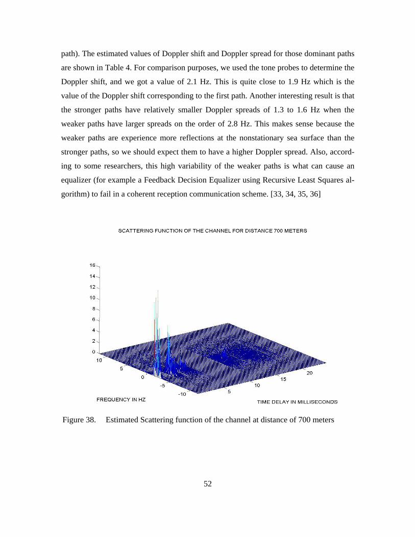
path). The estimated values of Doppler shift and Doppler spread for those dominant paths
are shown in Table 4. For comparison purposes, we used the tone probes to determine the
Doppler shift, and we got a value of 2.1 Hz. This is quite close to 1.9 Hz which is the
value of the Doppler shift corresponding to the first path. Another interesting result is that
the stronger paths have relatively smaller Doppler spreads of 1.3 to 1.6 Hz when the
weaker paths have larger spreads on the order of 2.8 Hz. This makes sense because the
weaker paths are experience more reflections at the nonstationary sea surface than the
stronger paths, so we should expect them to have a higher Doppler spread. Also, accord-
ing to some researchers, this high variability of the weaker paths is what can cause an
equalizer (for example a Feedback Decision Equalizer using Recursive Least Squares al-
gorithm) to fail in a coherent reception communication scheme. [33, 34, 35, 36]
Figure 38. Estimated Scattering function of the channel at distance of 700 meters
52
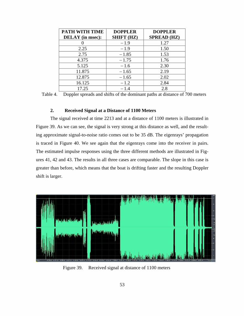
PATH WITH TIME DELAY (in msec):
DOPPLER SHIFT (HZ)
DOPPLER SPREAD (HZ)
0 −1.9 1.27 2.25 −1.9 1.50 2.75 −1.85 1.53 4.375 −1.75 1.76 5.125 −1.6 2.30 11.875 −1.65 2.19 12.875 −1.65 2.02 16.125 −1.2 2.84 17.25 −1.4 2.8
Table 4. Doppler spreads and shifts of the dominant paths at distance of 700 meters
2. Received Signal at a Distance of 1100 Meters The signal received at time 2213 and at a distance of 1100 meters is illustrated in
Figure 39. As we can see, the signal is very strong at this distance as well, and the result-
ing approximate signal-to-noise ratio comes out to be 35 dB. The eigenrays’ propagation
is traced in Figure 40. We see again that the eigenrays come into the receiver in pairs.
The estimated impulse responses using the three different methods are illustrated in Fig-
ures 41, 42 and 43. The results in all three cases are comparable. The slope in this case is
greater than before, which means that the boat is drifting faster and the resulting Doppler
shift is larger.
Figure 39. Received signal at distance of 1100 meters
53

Figure 40. Eigenrays plot for distance of 1100 meters
Figure 41. Estimated impulse response at 1100 meters
using LFM chirp
Figure 42. Estimated impulse response at 1100 meters
using DSSS signal in bandpass
54
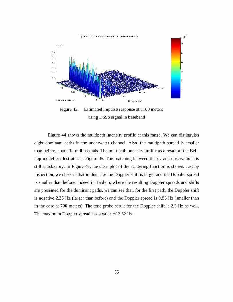
Figure 43. Estimated impulse response at 1100 meters
using DSSS signal in baseband
Figure 44 shows the multipath intensity profile at this range. We can distinguish
eight dominant paths in the underwater channel. Also, the multipath spread is smaller
than before, about 12 milliseconds. The multipath intensity profile as a result of the Bell-
hop model is illustrated in Figure 45. The matching between theory and observations is
still satisfactory. In Figure 46, the clear plot of the scattering function is shown. Just by
inspection, we observe that in this case the Doppler shift is larger and the Doppler spread
is smaller than before. Indeed in Table 5, where the resulting Doppler spreads and shifts
are presented for the dominant paths, we can see that, for the first path, the Doppler shift
is negative 2.25 Hz (larger than before) and the Doppler spread is 0.83 Hz (smaller than
in the case at 700 meters). The tone probe result for the Doppler shift is 2.3 Hz as well.
The maximum Doppler spread has a value of 2.62 Hz.
55

Figure 44. Multipath Intensity Profile at 1100 meters using DSSS signal in baseband
Figure 45. Multipath Intensity Profile at 1100 meters - Bellhop theoretical estimate
Figure 46. Estimated Scattering function of the channel at distance of 1100 meters
56

PATH WITH TIME DELAY (in msec):
DOPPLER SHIFT (HZ)
DOPPLER SPREAD (HZ)
0 −2.25 0.83 1.5 −2.15 1.50
2.875 −2.05 1.70 3.25 −2.1 1.84 7.625 −1.8 2.25 8.125 −1.8 2.13 10.75 −1.65 2.62 11.375 −1.6 2.40
Table 5. Doppler spreads and shifts of the dominant paths for distance of 1100 meters
3. Received Signal at a Distance of 1650 Meters
The signal received at time 2243 and at a distance of 1650 meters is illustrated in
Figure 47. As we can see, the signal is strong at this distance as well, and the resulting
signal-to-noise ratio is approximately 31 dB. In Figure 48 the eigenrays’ propagation,
modeled by the Bellhop numerical analysis, is traced. In this case too, the rays arrive in
pairs at the receiver, but the effect of attenuation is much stronger, and in the actual im-
pulse response plot those pairs are less distinguishable. The estimated impulse responses
using the three different methods are presented in Figures 49, 50 and 51. The results in all
three cases are consistent. The slope in this case is even greater than in two previous
cases, which means that the boat is drifting even faster and the resulting Doppler shift is
larger.
57
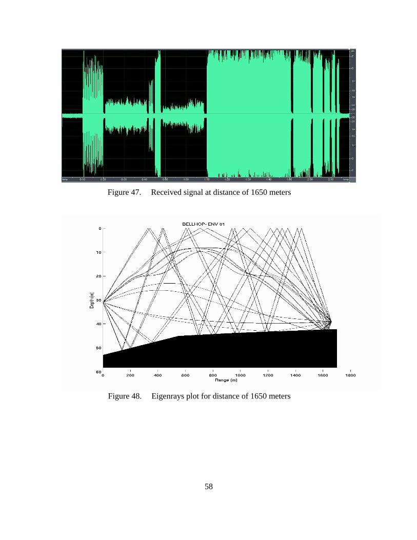
Figure 47. Received signal at distance of 1650 meters
Figure 48. Eigenrays plot for distance of 1650 meters
58
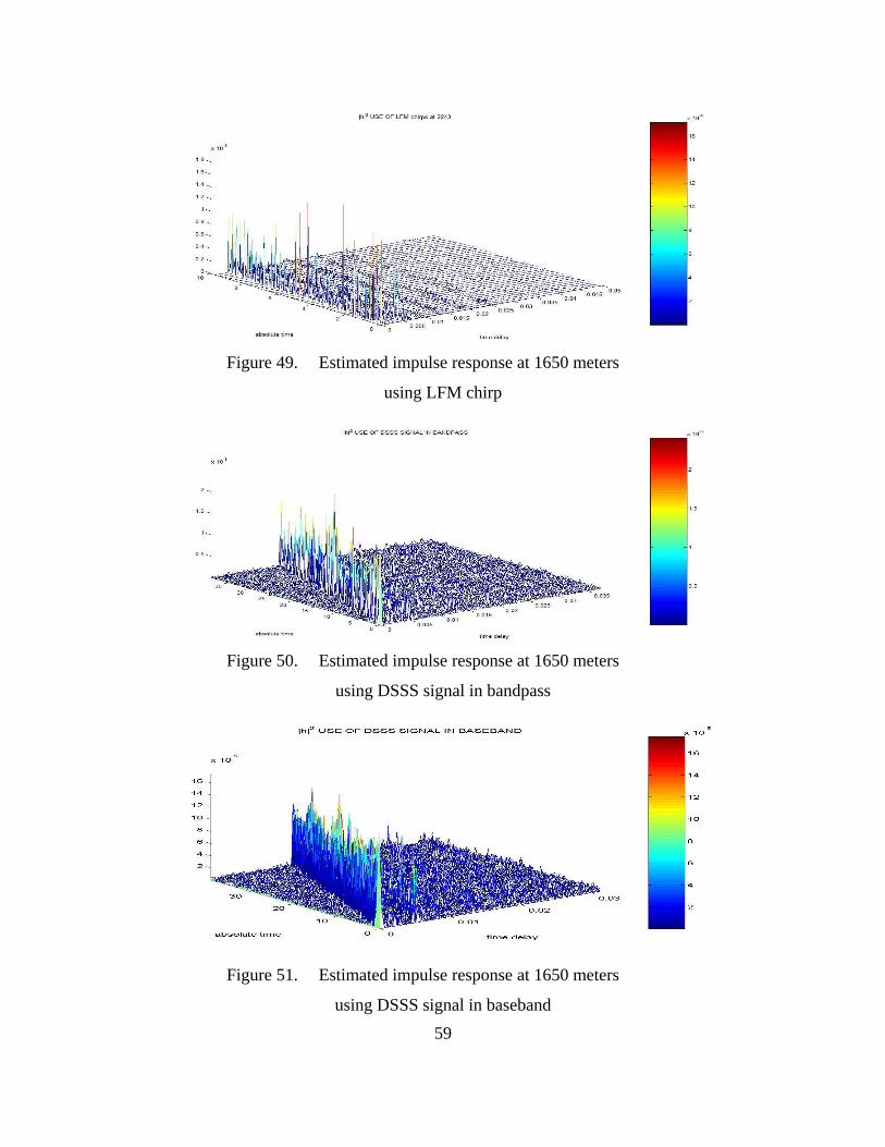
Figure 49. Estimated impulse response at 1650 meters
using LFM chirp
Figure 50. Estimated impulse response at 1650 meters
using DSSS signal in bandpass
Figure 51. Estimated impulse response at 1650 meters
using DSSS signal in baseband 59
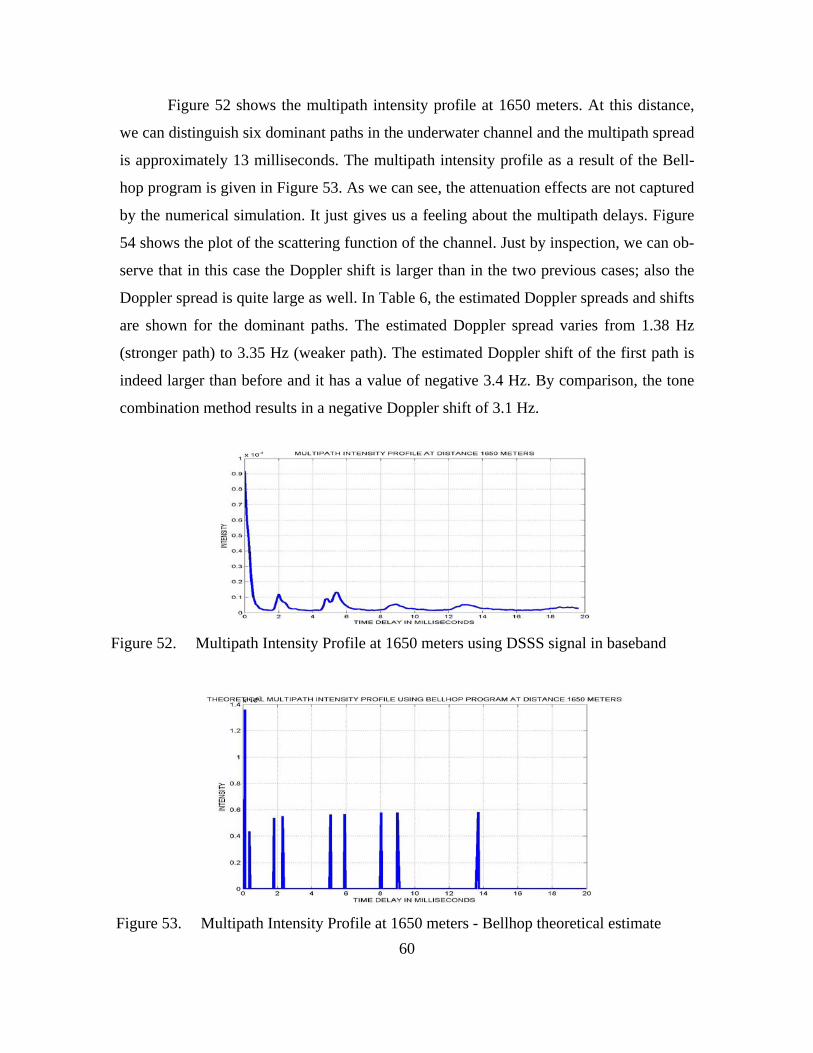
Figure 52 shows the multipath intensity profile at 1650 meters. At this distance,
we can distinguish six dominant paths in the underwater channel and the multipath spread
is approximately 13 milliseconds. The multipath intensity profile as a result of the Bell-
hop program is given in Figure 53. As we can see, the attenuation effects are not captured
by the numerical simulation. It just gives us a feeling about the multipath delays. Figure
54 shows the plot of the scattering function of the channel. Just by inspection, we can ob-
serve that in this case the Doppler shift is larger than in the two previous cases; also the
Doppler spread is quite large as well. In Table 6, the estimated Doppler spreads and shifts
are shown for the dominant paths. The estimated Doppler spread varies from 1.38 Hz
(stronger path) to 3.35 Hz (weaker path). The estimated Doppler shift of the first path is
indeed larger than before and it has a value of negative 3.4 Hz. By comparison, the tone
combination method results in a negative Doppler shift of 3.1 Hz.
Figure 52. Multipath Intensity Profile at 1650 meters using DSSS signal in baseband
Figure 53. Multipath Intensity Profile at 1650 meters - Bellhop theoretical estimate 60
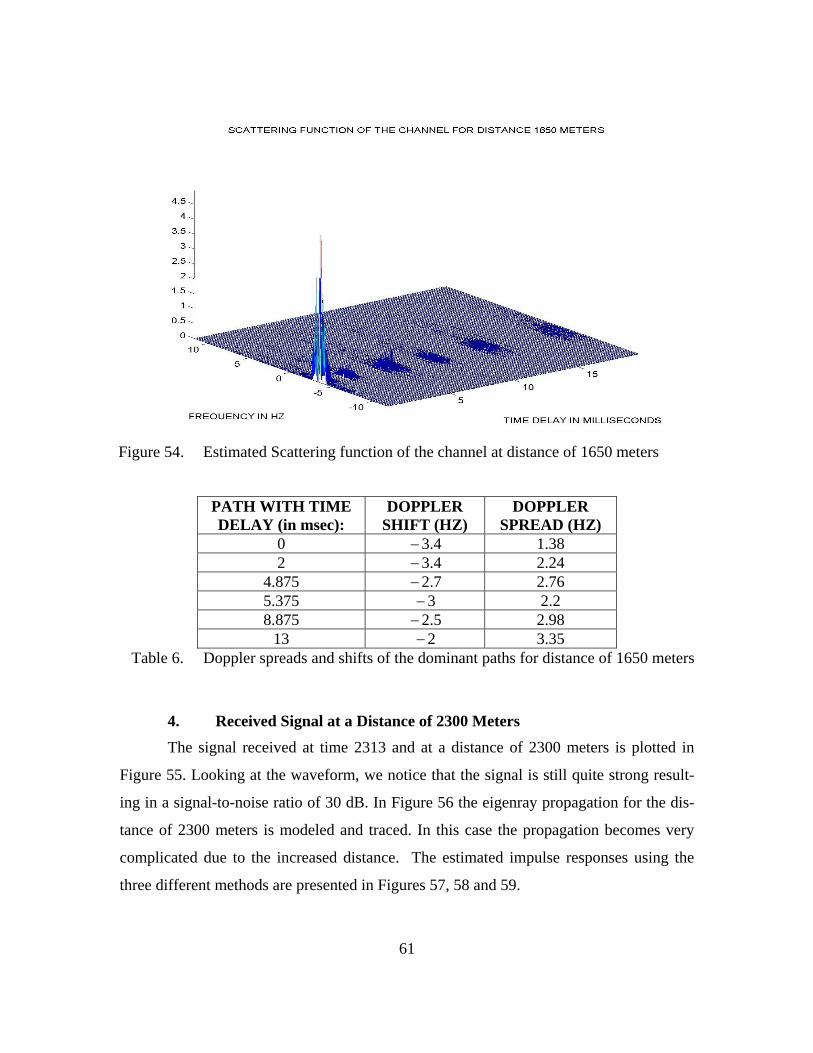
Figure 54. Estimated Scattering function of the channel at distance of 1650 meters
PATH WITH TIME DELAY (in msec):
DOPPLER SHIFT (HZ)
DOPPLER SPREAD (HZ)
0 −3.4 1.38 2 −3.4 2.24
4.875 −2.7 2.76 5.375 −3 2.2 8.875 −2.5 2.98
13 −2 3.35 Table 6. Doppler spreads and shifts of the dominant paths for distance of 1650 meters
4. Received Signal at a Distance of 2300 Meters The signal received at time 2313 and at a distance of 2300 meters is plotted in
Figure 55. Looking at the waveform, we notice that the signal is still quite strong result-
ing in a signal-to-noise ratio of 30 dB. In Figure 56 the eigenray propagation for the dis-
tance of 2300 meters is modeled and traced. In this case the propagation becomes very
complicated due to the increased distance. The estimated impulse responses using the
three different methods are presented in Figures 57, 58 and 59.
61

Figure 55. Received signal at distance of 2300 meters
Figure 56. Eigenrays plot for distance of 2300 meters
62

Figure 57. Estimated impulse response at 2300 meters
using LFM chirp
Figure 58. Estimated impulse response at 2300 meters
using DSSS signal in bandpass
Figure 59. Estimated impulse response at 2300 meters
using DSSS signal in baseband
63

The multipath intensity profile at 2300 meters is shown in Figure 60. At this dis-
tance, we can distinguish eight dominant paths in the underwater channel, and the multi-
path spread is about 10.5 milliseconds. The multipath intensity profile as a result of the
Bellhop model is illustrated in Figure 61. The result is quite similar except that the paths
corresponding to time delays 3.25 and 3.625 msecs are absent from the model. Figure 62
indicates the scattering function of the channel. Just by inspection we conclude that there
is a strong negative Doppler shift and a few dominant paths. In Table 7, the estimated
Doppler spreads and shifts are presented for the dominant paths. The estimated Doppler
spread varies from 0.89 Hz (stronger path) to 2.85 Hz (weaker path). We estimate that the
first path has a negative Doppler shift with a value of 3.2 Hz. By comparison, the tone
combination method results in a negative Doppler shift of 3.1 Hz.
Figure 60. Multipath Intensity Profile at 2300 meters using DSSS signal in baseband
Figure 61. Multipath Intensity Profile at 2300 meters - Bellhop theoretical estimate
64
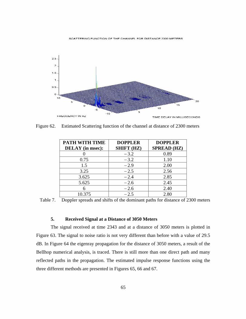
Figure 62. Estimated Scattering function of the channel at distance of 2300 meters
PATH WITH TIME DELAY (in msec):
DOPPLER SHIFT (HZ)
DOPPLER SPREAD (HZ)
0 −3.2 0.89 0.75 −3.2 1.10 1.5 −2.9 2.00 3.25 −2.5 2.56 3.625 −2.4 2.85 5.625 −2.6 2.45
6 −2.6 2.40 10.375 −2.5 2.80
Table 7. Doppler spreads and shifts of the dominant paths for distance of 2300 meters
5. Received Signal at a Distance of 3050 Meters The signal received at time 2343 and at a distance of 3050 meters is plotted in
Figure 63. The signal to noise ratio is not very different than before with a value of 29.5
dB. In Figure 64 the eigenray propagation for the distance of 3050 meters, a result of the
Bellhop numerical analysis, is traced. There is still more than one direct path and many
reflected paths in the propagation. The estimated impulse response functions using the
three different methods are presented in Figures 65, 66 and 67.
65

Figure 63. Received signal at distance of 3050 meters
Figure 64. Eigenrays plot for distance of 3050 meters
66

Figure 65. Estimated impulse response at 3050 meters
using LFM chirp
Figure 66. Estimated impulse response at 3050 meters
using DSSS signal in bandpass
Figure 67. Estimated impulse response at 3050 meters
using DSSS signal in baseband
67

The multipath intensity profile at 3050 meters is plotted in Figure 68. It is inter-
esting to notice that at this distance, the multipath effect is almost negligible since there
are only two dominant paths in the underwater channel. More specifically, the channel
has one strong path and one very weak (its intensity is equal to one tenth of that of the
strong), so the multipath spread is just 0.6 milliseconds. The Bellhop model shown in
Figure 69 shows many arrivals after the measured multipath spread of the channel. Proba-
bly those arrivals are very weak due to the multiple reflections. Figure 70 indicates the
scattering function of the channel with the two paths. In Table 8, the estimated Doppler
spreads and shifts are presented for the two paths. The estimated Doppler spreads are
0.53 and 1.44 corresponding to the strong and weak path of the channel, respectively. The
Doppler shift of the first path is negative with a value of 3.5 Hz. By comparison, the tone
combination method results in a negative Doppler shift of 3.3 Hz.
Figure 68. Multipath Intensity Profile at 3050 meters using DSSS signal in baseband
Figure 69. Multipath Intensity Profile at 3050 meters - Bellhop theoretical estimate
68
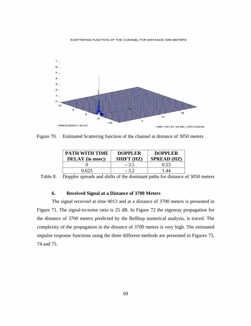
Figure 70. Estimated Scattering function of the channel at distance of 3050 meters
PATH WITH TIME DELAY (in msec):
DOPPLER SHIFT (HZ)
DOPPLER SPREAD (HZ)
0 −3.5 0.53 0.625 −3.2 1.44
Table 8. Doppler spreads and shifts of the dominant paths for distance of 3050 meters
6. Received Signal at a Distance of 3700 Meters
The signal received at time 0013 and at a distance of 3700 meters is presented in
Figure 71. The signal-to-noise ratio is 25 dB. In Figure 72 the eigenray propagation for
the distance of 3700 meters predicted by the Bellhop numerical analysis, is traced. The
complexity of the propagation in the distance of 3700 meters is very high. The estimated
impulse response functions using the three different methods are presented in Figures 73,
74 and 75.
69

Figure 71. Received signal at distance of 3700 meters
Figure 72. Eigenrays plot for distance of 3700 meters
70
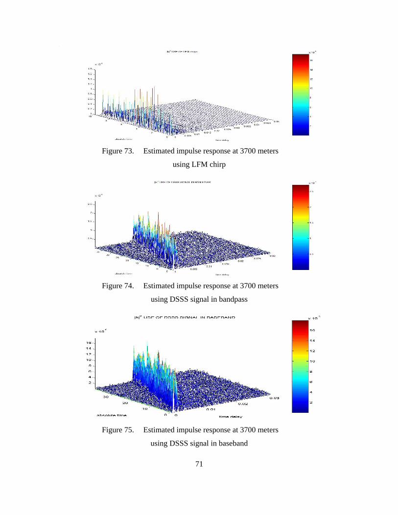
Figure 73. Estimated impulse response at 3700 meters
using LFM chirp
Figure 74. Estimated impulse response at 3700 meters
using DSSS signal in bandpass
Figure 75. Estimated impulse response at 3700 meters
using DSSS signal in baseband
71

The multipath intensity profile at 3700 meters is illustrated in Figure 76. The di-
rect path is weaker, and the relative strengths of the later paths are more significant. We
have four dominant paths (two strong and two weak). The resulting multipath spread has
a value of 3.5 milliseconds. The Bellhop model shown in Figure 77 has a good match in
the first 4 milliseconds but, after that value of delay, it shows 3 arrivals that we cannot
detect in the measured result. It seems that they attenuated due to the multiple reflections.
In Figure 78, the scattering function for this case is illustrated. In Table 9, the estimated
Doppler spreads and shifts are presented for the four paths. The estimated Doppler
spreads vary from 0.93 to 2.71 Hz, corresponding to the strongest and the weakest path,
respectively. The Doppler shift of the first path is negative with a value of 3.5 Hz. By
comparison, the tone probes show a negative Doppler shift of 3.6 Hz.
Figure 76. Multipath Intensity Profile at 3700 meters using DSSS signal in baseband
Figure 77. Multipath Intensity Profile at 3700 meters - Bellhop theoretical estimate
72
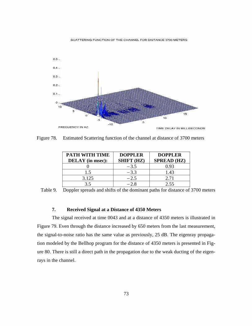
Figure 78. Estimated Scattering function of the channel at distance of 3700 meters
PATH WITH TIME DELAY (in msec):
DOPPLER SHIFT (HZ)
DOPPLER SPREAD (HZ)
0 −3.5 0.93 1.5 −3.3 1.43
3.125 −2.5 2.71 3.5 −2.8 2.55
Table 9. Doppler spreads and shifts of the dominant paths for distance of 3700 meters
7. Received Signal at a Distance of 4350 Meters The signal received at time 0043 and at a distance of 4350 meters is illustrated in
Figure 79. Even through the distance increased by 650 meters from the last measurement,
the signal-to-noise ratio has the same value as previously, 25 dB. The eigenray propaga-
tion modeled by the Bellhop program for the distance of 4350 meters is presented in Fig-
ure 80. There is still a direct path in the propagation due to the weak ducting of the eigen-
rays in the channel.
73

Figure 79. Received signal at distance of 4350 meters
Figure 80. Eigenrays plot for distance of 4350 meters
74

Figure 81. Estimated impulse response at 4350 meters
using LFM chirp
Figure 82. Estimated impulse response at 4350 meters using DSSS signal in bandpass
Figure 83. Estimated impulse response at 4350 meters using DSSS signal in baseband
75

The multipath intensity profile of the channel at 4350 meters is illustrated in Fig-
ure 84. The multipath effect at this distance is getting very weak again since, even if we
have three dominant paths in this case, the relative intensities of the second and third
paths, in contrast with the first path, are very small. The resulting multipath spread has a
value of 2.4 milliseconds. The Bellhop model shown in Figure 85 does a very good fit to
the measured result, except the peak at 8.7 msecs delay which is probably attenuated in
the real propagation. In Figure 86, the scattering function of the channel is illustrated. In
Table 10, we summarize the estimated Doppler spreads and shifts of the three paths. The
estimated Doppler spreads vary from 0.66 to 2.06 Hz, corresponding to the strongest and
the weakest path respectively. The Doppler shift of the first path is negative with a value
of 3.15 Hz. For comparison, the tone probe show a negative Doppler shift of 3.4 Hz.
Figure 84. Multipath Intensity Profile at 4350 meters using DSSS signal in baseband
Figure 85. Multipath Intensity Profile at 4350 meters - Bellhop theoretical estimate
76

Figure 86. Estimated Scattering function of the channel at distance of 4350 meters
PATH WITH TIME DELAY (in msec):
DOPPLER SHIFT (HZ)
DOPPLER SPREAD (HZ)
0 −3.15 0.66 1.125 −3 1.30 2.375 −3 2.06
Table 10. Doppler spreads and shifts of the dominant paths for distance of 4350 meters
8. Received Signal at a Distance of 5000 Meters The signal received at time 0113 and at a distance of 5000 meters is illustrated in
Figure 87. This is the most interesting case of all since we have a very sudden and drastic
reduction of the signal strength. The distance increased by 650 meters and the signal-to-
noise ratio reduced by 9 dB (a factor of 8!). The SNR in this case is 16 dB, easily visible
by comparing Figure 87 with Figure 79. More likely, the dominant path is beginning to
be unsupported by the channel geometry. The eigenray propagation modeled by the Bell-
hop program for the distance of 5000 meters is presented in Figure 88. The plot is very
crowded with all the eigenrays in this distance, so we can not make any conclusion for
the propagation with respect to the drastic drop of the SNR.
77

Figure 87. Received signal at distance of 5000 meters
Figure 88. Eigenrays plot for distance of 5000 meters
78

Figure 89. Estimated impulse response at 5000 meters
using LFM chirp
Figure 90. Estimated impulse response at 5000 meters using DSSS signal in bandpass
Figure 91. Estimated impulse response at 5000 meters using DSSS signal in baseband
79
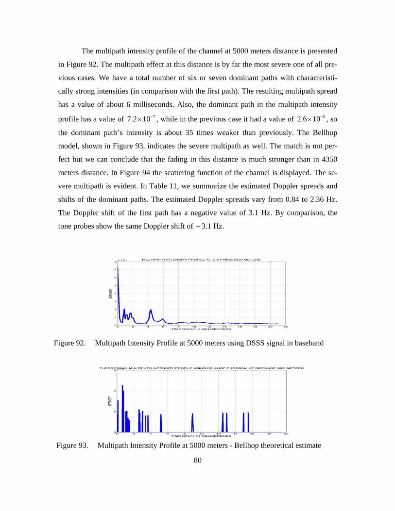
The multipath intensity profile of the channel at 5000 meters distance is presented
in Figure 92. The multipath effect at this distance is by far the most severe one of all pre-
vious cases. We have a total number of six or seven dominant paths with characteristi-
cally strong intensities (in comparison with the first path). The resulting multipath spread
has a value of about 6 milliseconds. Also, the dominant path in the multipath intensity
profile has a value of , while in the previous case it had a value of 77.2 10−× 52.6 10−× , so
the dominant path’s intensity is about 35 times weaker than previously. The Bellhop
model, shown in Figure 93, indicates the severe multipath as well. The match is not per-
fect but we can conclude that the fading in this distance is much stronger than in 4350
meters distance. In Figure 94 the scattering function of the channel is displayed. The se-
vere multipath is evident. In Table 11, we summarize the estimated Doppler spreads and
shifts of the dominant paths. The estimated Doppler spreads vary from 0.84 to 2.36 Hz.
The Doppler shift of the first path has a negative value of 3.1 Hz. By comparison, the
tone probes show the same Doppler shift of −3.1 Hz.
Figure 92. Multipath Intensity Profile at 5000 meters using DSSS signal in baseband
Figure 93. Multipath Intensity Profile at 5000 meters - Bellhop theoretical estimate
80

Figure 94. Estimated Scattering function of the channel at distance of 5000 meters
PATH WITH TIME DELAY (in msec):
DOPPLER SHIFT (HZ)
DOPPLER SPREAD (HZ)
0 −3.1 0.84 0.875 −2.95 1.51 1.25 −2.7 1.83 1.75 −2.8 1.84 4.375 −2.9 1.7 5.875 −2.6 2.36
Table 11. Doppler spreads and shifts of the dominant paths for distance of 5000 meters
9. Received Signal at a Distance of 5750 Meters The signal received at time 0143 and at a distance of 5750 meters is illustrated in
Figure 95. In this case the received signal power reduces even more resulting in a lower
signal-to-noise ratio of 13 dB. The plots of the impulse response function are presented in
Figures 96, 97 and 98.
81

Figure 95. Received signal at distance of 5750 meters
Figure 96. Estimated impulse response at 5750 meters
using LFM chirp
Figure 97. Estimated impulse response at 5750 meters using DSSS signal in bandpass
82
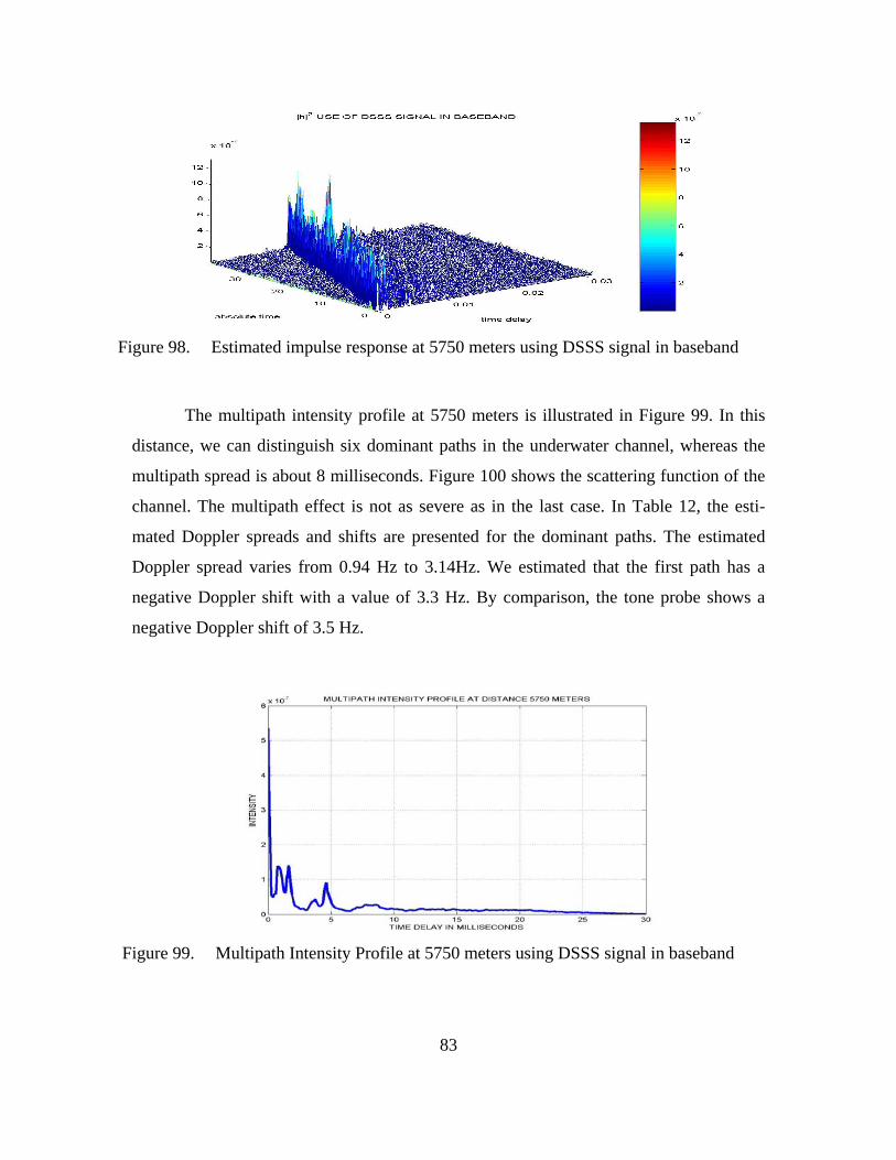
Figure 98. Estimated impulse response at 5750 meters using DSSS signal in baseband
The multipath intensity profile at 5750 meters is illustrated in Figure 99. In this
distance, we can distinguish six dominant paths in the underwater channel, whereas the
multipath spread is about 8 milliseconds. Figure 100 shows the scattering function of the
channel. The multipath effect is not as severe as in the last case. In Table 12, the esti-
mated Doppler spreads and shifts are presented for the dominant paths. The estimated
Doppler spread varies from 0.94 Hz to 3.14Hz. We estimated that the first path has a
negative Doppler shift with a value of 3.3 Hz. By comparison, the tone probe shows a
negative Doppler shift of 3.5 Hz.
Figure 99. Multipath Intensity Profile at 5750 meters using DSSS signal in baseband
83

Figure 100. Estimated Scattering function of the channel at distance of 5750 meters
PATH WITH TIME DELAY (in msec):
DOPPLER SHIFT (HZ)
DOPPLER SPREAD (HZ)
0 −3.3 0.94 0.75 −3.15 1.57 1.625 −3.15 1.50 3.75 −2.55 2.52 4.625 −2.95 1.91 7.75 −2.3 3.14
Table 12. Doppler spreads and shifts of the dominant paths for distance of 5750 meters
10. Received Signal at a Distance of 6550 Meters The signal received at time 0213 and at a distance of 6550 meters is illustrated in
Figure 101. At this distance, we are very close to losing the signal inside the noise.
Probably that distance would be the communication limit of this underwater environment.
The signal-to-noise ratio at the distance of 6.5 kilometers is about 7 dB. The plots of the
impulse response function for this case are presented in Figures 102, 103 and 104.
84
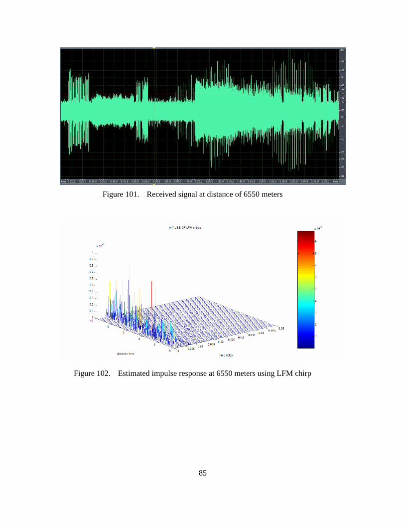
Figure 101. Received signal at distance of 6550 meters
Figure 102. Estimated impulse response at 6550 meters using LFM chirp
85
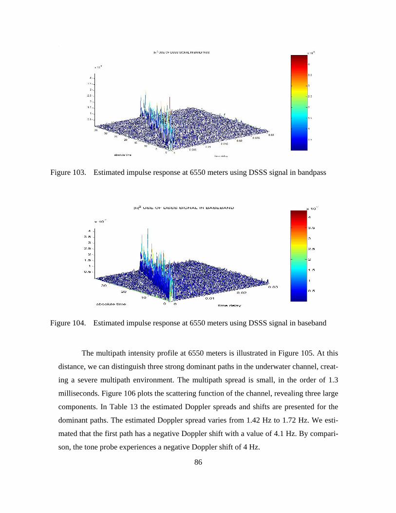
Figure 103. Estimated impulse response at 6550 meters using DSSS signal in bandpass
Figure 104. Estimated impulse response at 6550 meters using DSSS signal in baseband
The multipath intensity profile at 6550 meters is illustrated in Figure 105. At this
distance, we can distinguish three strong dominant paths in the underwater channel, creat-
ing a severe multipath environment. The multipath spread is small, in the order of 1.3
milliseconds. Figure 106 plots the scattering function of the channel, revealing three large
components. In Table 13 the estimated Doppler spreads and shifts are presented for the
dominant paths. The estimated Doppler spread varies from 1.42 Hz to 1.72 Hz. We esti-
mated that the first path has a negative Doppler shift with a value of 4.1 Hz. By compari-
son, the tone probe experiences a negative Doppler shift of 4 Hz.
86
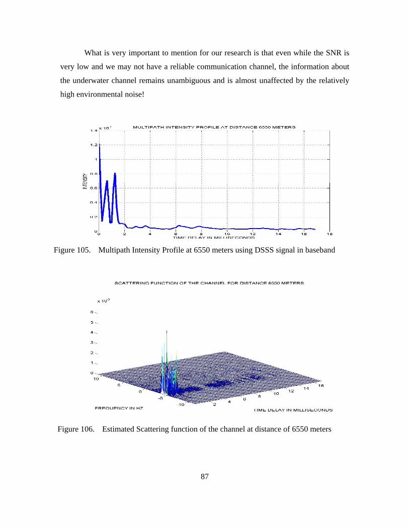
What is very important to mention for our research is that even while the SNR is
very low and we may not have a reliable communication channel, the information about
the underwater channel remains unambiguous and is almost unaffected by the relatively
high environmental noise!
Figure 105. Multipath Intensity Profile at 6550 meters using DSSS signal in baseband
Figure 106. Estimated Scattering function of the channel at distance of 6550 meters
87

PATH WITH TIME DELAY (in msec):
DOPPLER SHIFT (HZ)
DOPPLER SPREAD (HZ)
0 −4.1 1.42 0.625 −4 1.73 1.25 −4 1.72
Table 13. Doppler spreads and shifts of the dominant paths for distance of 6550 meters
11. Summary of the Results
Figure 107 presents a summary of the multipath intensity profiles for the ten dif-
ferent cases of varying distance. Figure 108 presents a summary of the channel scattering
functions for the ten different ranges.
Figure 107. Summary of the MIPs for the 10 different cases
88
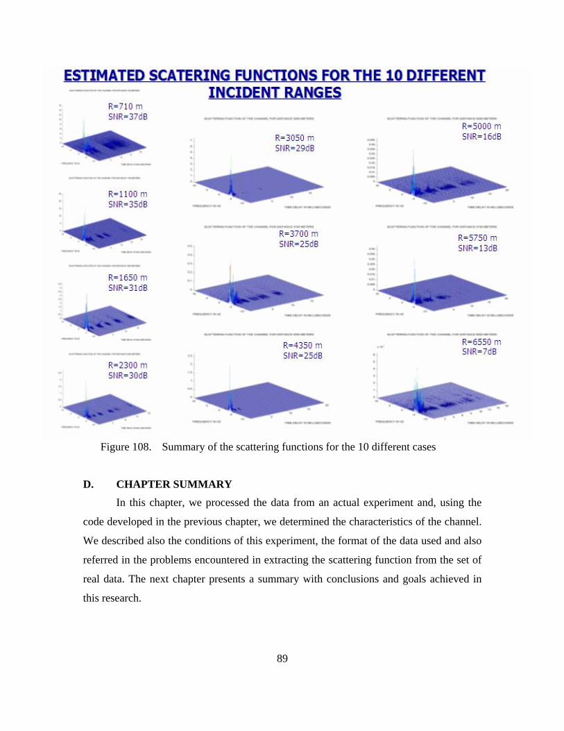
Figure 108. Summary of the scattering functions for the 10 different cases
D. CHAPTER SUMMARY
In this chapter, we processed the data from an actual experiment and, using the
code developed in the previous chapter, we determined the characteristics of the channel.
We described also the conditions of this experiment, the format of the data used and also
referred in the problems encountered in extracting the scattering function from the set of
real data. The next chapter presents a summary with conclusions and goals achieved in
this research.
89

90
THIS PAGE INTENTIONALLY LEFT BLANK

91
VI. CONCLUSIONS AND FUTURE WORK
A. CONCLUSIONS This thesis examined the behavior of the underwater channel in which the Seaweb
communication network operates. After developing the theory describing the underwater
channel from both physics and electrical engineering perspectives, and discussing how
the channel characteristics affect the acoustic communication signal, we described an ef-
ficient method of measuring those characteristics, even in the presence of noise.
The next step was to simulate a time-varying underwater channel with multipath
characteristics. After passing a bandpass communication signal through this channel, we
applied the method developed in the previous chapter to measure the characteristics of
the artificial channel. The purpose of this action was twofold: first, the simulated channel
served as a test channel to ensure that the method works as expected and secondly to ob-
serve the influence of the gradually increased noise levels on the results of the estimation.
The results were quite satisfactory since they were accurate even for signal to
noise ratio of 7 dB. Finally, we described an actual ocean experiment and the various
types of signals sent as channel probes. Each signal type served a different purpose with
respect to determining the effect of the channel on the acoustic communication signal.
The different types of signal sent gave us the opportunity to examine other ways of chan-
nel estimation besides the one we described in Chapter IV.
The key findings from this work are as follows:
• LFM chirps and the matched filter method gave us a very clear picture for
the estimated impulse response of the channel. However, the low meas-
urement rate of this method led to great aliasing in the scattering function,
which made Doppler estimation impossible.
• The DSSS method worked very well in both the bandpass and baseband
cases, so that the transition from bandpass to baseband prior to channel es-
timation is unnecessary.

92
• The results of the DSSS method gave a noisy picture for the impulse re-
sponse because of the format of the DSSS signal. The multipath intensity
profile on the other hand gave a good estimate of the channel (still noisy).
The estimate of the scattering function from the DSSS method came out
very clear and very accurate, giving us unambiguous information for the
channel.
• Each of the different paths in the multipath has a different value of Dop-
pler shift and Doppler spread. The weaker components of the impulse re-
sponse usually have higher Doppler spreads than the stronger ones, and
the impulse response component corresponding to the first path usually
has the highest Doppler shift.
• The tonal comb signal gave us a value of Doppler shift very close or ex-
actly the same as that of the impulse response component corresponding to
the first path.
B. FUTURE WORK Since we have shown the feasibility of measuring the important characteristics of
the underwater channel, the next step is to implement the DSSS signal and the appropri-
ate algorithm inside the Seaweb modem. A natural implementation is to send a known
DSSS signal in the beginning of the communication (inside the RTS transmission).
A separate important task will be associating the underwater channel types with
the available communication schemes and their parameters such as frequency band of op-
eration, modulation scheme (coherent, non coherent and specific type), data rate, modem
output power, and error correction coding type, which will give us the minimum prob-
ability of error. The match up can be done by researching the several experiments that
have been done in different ocean environments, by organizing new ones towards this
specific goal, and by simulating the communication system. We anticipate that there must
be a limiting case of severity in the channel conditions beyond which we cannot use any
phase coherent techniques with equalization and we are compelled to use the more robust
93
non-coherent FSK, since this appears to be less susceptible to channel impairments and
seems to provide robust communications and relatively high data rates.
The ultimate scope of future work is to build an adaptive modem that will esti-
mate the character of the channel using the DSSS method and, based on that, will decide
on the communication parameters which optimize communication between neighboring
pairs of Seaweb nodes.

94
THIS PAGE INTENTIONALLY LEFT BLANK

95
APPENDIX. MATLAB CODES
In this appendix, we present the Matlab codes used in this work to generate the re-
sults and the plots for the artificial and the actual channel.
% GENERATION OF DSSS (GOLD CODE WITH LENGTH 2047) % AND PROBE SIGNAL WITH LENGTH 8 bits clc clear close all format long load gold2047_1 code1=code(1,:); code2=code(2,:); s1=sign(randn(1,8)); sa=(code1'*s1)+(i*code2'*s1); s=reshape(sa,1,2047*length(s1)); s=s+0.1*randn(1,2047*length(s1)); % UPSAMPLING THE DATA % sampleperchip = ones(1,1); % hlp = sampleperchip'*s2; % s = reshape(hlp, 1 ,prod(size(hlp))); s=s'; % CREATE DATA FOR USE s1=[]; for i=1:201 ss(i,i)=0; s1=[s1 s(i,1)]; ss(i,:)=s1; end ss=conj(ss); sa=[]; for i=1:(200) sa=[sa ; s(1:200)']; end
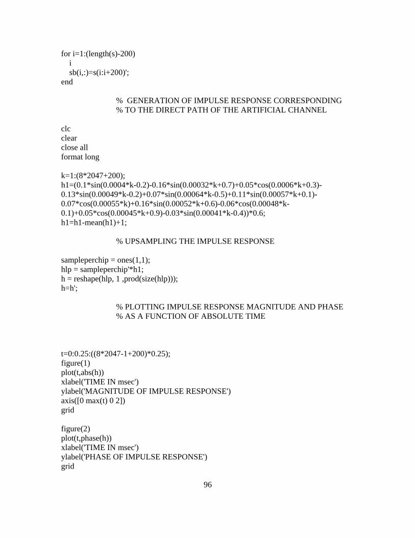
96
for i=1:(length(s)-200) i sb(i,:)=s(i:i+200)'; end % GENERATION OF IMPULSE RESPONSE CORRESPONDING % TO THE DIRECT PATH OF THE ARTIFICIAL CHANNEL clc clear close all format long k=1:(8*2047+200); h1=(0.1*sin(0.0004*k-0.2)-0.16*sin(0.00032*k+0.7)+0.05*cos(0.0006*k+0.3)-0.13*sin(0.00049*k-0.2)+0.07*sin(0.00064*k-0.5)+0.11*sin(0.00057*k+0.1)-0.07*cos(0.00055*k)+0.16*sin(0.00052*k+0.6)-0.06*cos(0.00048*k-0.1)+0.05*cos(0.00045*k+0.9)-0.03*sin(0.00041*k-0.4))*0.6; h1=h1-mean(h1)+1; % UPSAMPLING THE IMPULSE RESPONSE sampleperchip = ones(1,1); hlp = sampleperchip'*h1; h = reshape(hlp, 1 ,prod(size(hlp))); h=h'; % PLOTTING IMPULSE RESPONSE MAGNITUDE AND PHASE % AS A FUNCTION OF ABSOLUTE TIME t=0:0.25:((8*2047-1+200)*0.25); figure(1) plot(t,abs(h)) xlabel('TIME IN msec') ylabel('MAGNITUDE OF IMPULSE RESPONSE') axis([0 max(t) 0 2]) grid figure(2) plot(t,phase(h)) xlabel('TIME IN msec') ylabel('PHASE OF IMPULSE RESPONSE') grid
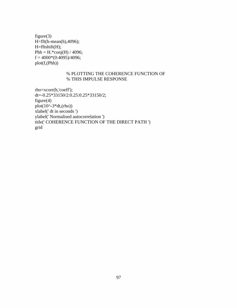
97
figure(3) H=fft(h-mean(h),4096); H=fftshift(H); Phh = H.*conj(H) / 4096; f = 4000*(0:4095)/4096; plot(f,(Phh)) % PLOTTING THE COHERENCE FUNCTION OF % THIS IMPULSE RESPONSE rho=xcorr(h,'coeff'); dt=-0.25*33150/2:0.25:0.25*33150/2; figure(4) plot(10^-3*dt,(rho)) xlabel(' dt in seconds ') ylabel(' Normalised autocorrelation ') title(' COHERENCE FUNCTION OF THE DIRECT PATH ') grid

98
% GENERATION OF IMPULSE RESPONSE CORRE % SPONDING TO THE SECOND % PATH OF THE ARTIFICIAL CHANNEL clc clear close all format long k=1:(2047*8+200); h1=(-0.2*sin(0.00035*k-0.2)-0.1*sin(0.00036*k+0.9)+0.09*cos(0.000411*k+0.6)-0.09*sin(0.000361*k-0.4)+0.13*sin(0.00047*k-.5)+0.15*sin(0.00052*k+0.3)-0.13*cos(0.00048*k-0.6)-0.07*sin(0.00057*k+0.7)-0.06*cos(0.00046*k)-0.04*cos(0.00043*k-0.6)-0.04*sin(0.00037*k-0.4))*1.3; h1=h1-mean(h1)+0.5; % UPSAMPLING THE IMPULSE RESPONSE sampleperchip = ones(1,1); hlp = sampleperchip'*h1; h = reshape(hlp, 1 ,prod(size(hlp))); ha=h'; % PLOTTING IMPULSE RESPONSE MAGNITUDE AND % PHASE AS A FUNCTION OF ABSOLUTE TIME t=0:0.25:((2047*8-1+200)*0.25); figure(1) plot(t,abs(ha)) xlabel('TIME IN msec') ylabel('MAGNITUDE OF IMPULSE RESPONSE') axis([0 max(t) 0 2]) grid figure(2) plot(t,phase(ha)) xlabel('TIME IN msec') ylabel('PHASE OF IMPULSE RESPONSE') grid figure(3) H=fft(ha-mean(ha),4096); H=fftshift(H);
Phh = H.*conj(H) / 4096;
99
f = 4000*(0:4095)/4096; plot(f,(Phh)) % PLOTTING THE COHERENCE FUNCTION OF THIS % IMPULSE RESPONSE rho=xcorr(ha,'coeff'); dt=-0.25*33150/2:0.25:0.25*33150/2; figure(4) plot(10^-3*dt,(rho)) xlabel(' dt in seconds ') ylabel(' Normalized autocorrelation ') title(' COHERENCE FUNCTION OF THE SECOND PATH (TIME DELAY 10 msecs) ') grid

100
% GENERATION OF IMPULSE RESPONSE CORRE- % SPONDING TO THE THIRD PATH OF THE ARTIFICIAL % CHANNEL
clc clear close all format long k=1:(2047*8+200); h1=(0.1*sin(0.00030*k-0.4)-0.4*sin(0.00046*k+0.9)+0.07*cos(0.00028*k+0.3)+0.07*sin(0.00041*k-0.1)-0.14*sin(0.00035*k-.5)-0.18*sin(0.00026*k+0.1)+0.14*cos(0.00035*k-0.6)-0.08*sin(0.00037*k+0.7)+0.07*cos(0.00034*k-1.1)-0.09*cos(0.00029*k-0.5)-0.08*sin(0.00036*k-0.2))*0.5; h1=h1-mean(h1)+0.2; % UPSAMPLING THE IMPULSE RESPONSE sampleperchip = ones(1,1); hlp = sampleperchip'*h1; h = reshape(hlp, 1 ,prod(size(hlp))); hb=h'; % PLOTTING IMPULSE RESPONSE MAGNITUDE AND % PHASE AS A FUNCTION OF ABSOLUTE TIME t=0:0.25:((2047*8-1+200)*0.25); figure(1) plot(t,abs(hb)) xlabel('TIME IN msec') ylabel('MAGNITUDE OF IMPULSE RESPONSE') title('IMPULSE RESPONSE AT TIME DELAY 10 MILLISECONDS') axis([0 max(t) 0 1]) grid figure(2) plot(t,phase(hb)) xlabel('TIME IN msec') ylabel('PHASE OF IMPULSE RESPONSE') grid figure(3) H=fft(hb-mean(hb),4096); H=fftshift(H);

101
Phh = H.*conj(H) / 4096; f = 4000*(0:4095)/4096; plot(f,(Phh)) % PLOTTING THE COHERENCE FUNCTION OF THIS % IMPULSE RESPONSE rho=xcorr(hb,'coeff'); dt=-0.25*33150/2:0.25:0.25*33150/2; figure(4) plot(10^-3*dt,(rho)) xlabel(' dt in seconds ') ylabel(' Normalised autocorrelation ') title(' COHERENCE FUNCTION CORRESPONDING TO THE THIRD PATH (TIME DELAY 50 msecs) ') grid

102
% COMPARISON OF THE THREE COMPONENTS OF THE IM % PULSE RESPONSE OF THE ARTIFICIAL CHANNEL clc clear close all format long k=1:(2047*8+200); h1=(0.1*sin(0.00030*k-0.4)-0.4*sin(0.00046*k+0.9)+0.07*cos(0.00028*k+0.3)+0.07*sin(0.00041*k-0.1)-0.14*sin(0.00035*k-.5)-0.18*sin(0.00026*k+0.1)+0.14*cos(0.00035*k-0.6)-0.08*sin(0.00037*k+0.7)+0.07*cos(0.00034*k-1.1)-0.09*cos(0.00029*k-0.5)-0.08*sin(0.00036*k-0.2))*0.5; hb=h1-mean(h1)+0.2; h1=(-0.2*sin(0.00035*k-0.2)-0.1*sin(0.00036*k+0.9)+0.09*cos(0.000411*k+0.6)-0.09*sin(0.000361*k-0.4)+0.13*sin(0.00047*k-.5)+0.15*sin(0.00052*k+0.3)-0.13*cos(0.00048*k-0.6)-0.07*sin(0.00057*k+0.7)-0.06*cos(0.00046*k)-0.04*cos(0.00043*k-0.6)-0.04*sin(0.00037*k-0.4))*1.3; ha=h1-mean(h1)+0.5; h1=(0.1*sin(0.0004*k-0.2)-0.16*sin(0.00032*k+0.7)+0.05*cos(0.0006*k+0.3)-0.13*sin(0.00049*k-0.2)+0.07*sin(0.00064*k-0.5)+0.11*sin(0.00057*k+0.1)-0.07*cos(0.00055*k)+0.16*sin(0.00052*k+0.6)-0.06*cos(0.00048*k-0.1)+0.05*cos(0.00045*k+0.9)-0.03*sin(0.00041*k-0.4))*0.6; h=h1-mean(h1)+1; t=0:0.00025:((2047*8-1+200)*0.25/1000); figure(1) subplot(3,1,1) plot(t,abs(h)) title('IMPULSE RESPONSE AT TIME DELAY ZERO') axis([0 max(t) 0 2]) grid subplot(3,1,2) plot(t,abs(ha)) title('IMPULSE RESPONSE AT TIME DELAY 10 MILLISECONDS') ylabel('MAGNITUDE OF IMPULSE RESPONSE') axis([0 max(t) 0 2]) grid subplot(3,1,3)

103
plot(t,abs(hb)) xlabel('TIME IN SECONDS') title('IMPULSE RESPONSE AT TIME DELAY 50 MILLISECONDS') axis([0 max(t) 0 1]) grid htel=[h; zeros(39,16576); ha; zeros(159,16576); hb; zeros(1,16576)]; % MULTIPATH INTENSITY PROFILE OF THE ARTIFICIAL % CHANNEL figure(2) a=conj(htel).*htel; phih=0.5*sum(a')/16576; plot(0:0.25:201*0.25,phih) axis([-0.11 50.5 0 0.53]) grid title(' MULTIPATH INTENSITY PROFILE (MIP) ') xlabel(' TIME DELAY IN MILLISECONDS ') ylabel(' AVERAGE MULTIPATH INTENSITY ')
104
% TEST CHANNEL ESTIMATION clc clear close all load dataprosepejergasia; % DATA GENERATION load impulse1; % FIRST COMPONENT OF IMPULSE RESPONSE load impulse05; % SECOND COMPONENT OF IMPULSE RESPONSE load impulse02; % THIRD COMPONENT OF IMPULSE RESPONSE htel=[h.'; zeros(39,16576); ha.'; zeros(159,16576); hb.'; ]; % DATA PASSING THROUGH THE CHANNEL % RECEIVED SIGNAL GENERATION % PLUS AWGN s=fliplr(sb); ss=s(1,:); spro=zeros(200,201); for i=1:200 spro(201-i,:)=[ss(i+1:201) zeros(1,i)]; end st=s(16176,:); smeta=zeros(200,201); for i=1:200 smeta(i,:)=[zeros(1,i) st(1:201-i)]; end stel=[ spro ; s; smeta]; for i=1:16576 rcv(i)=stel(i,:)*htel(:,i); end rcv=rcv+0.44*(randn(1,16576)+j*randn(1,16576)); figure(1) plot(real(rcv),imag(rcv),'*') for i=1:8 c(i)=sb(2047*(i-1)+1);

105
end s1=-c./(1+j); load gold2047_1 code1=code(1,:); code2=code(2,:); sa=(code1'*s1)+(j*code2'*s1); s2=reshape(sa,1,2047*length(s1)); % UPSAMPLING THE DATA sampleperchip = ones(1,1); hlp = sampleperchip'*s2; sp = reshape(hlp, 1 ,prod(size(hlp))); sp=sp.'; % CHANNEL ESTIMATION sc=conj(sp); d=0; for g=210:100:14300 g d=d+1; for k=1:205 sum1=0; for m=1:2047 boh=rcv(g+m)*sc(g+m-k+1); sum1=boh+sum1; end hestim(d,k)=sum1/(2047*2); end end % PLOTTING THE ESTIMATE OF IMPULSE % RESPONSE AS WELL AS THE ACTUAL IMPULSE % RESPONSE FOR COMPARISON PURPOSES t=0:0.0025:0.0025*16575; t1=210*0.00025:0.025:14300*0.00025; figure(2) subplot(2,1,1) plot(t,h) title(' ACTUAL IMPULSE RESPONSE OF THE DIRECT PATH ') ylabel(' MAGNITUDE OF IMPULSE RESPONSE ')

106
grid hesta=abs(hestim(:,1)); subplot(2,1,2) plot(t1,hesta) title(' ESTIMATED IMPULSE RESPONSE OF THE DIRECT PATH ') xlabel(' ABSOLUTE TIME IN SECONDS ') ylabel(' MAGNITUDE OF IMPULSE RESPONSE ') axis([0 4.5 0.8 1.2]) grid figure(3) subplot(2,1,1) plot(t,ha) title(' ACTUAL IMPULSE RESPONSE OF THE SECOND PATH (TIME DELAY 10 mecs) ') ylabel(' MAGNITUDE OF IMPULSE RESPONSE ') grid hestb=hestim(:,41); subplot(2,1,2) plot(t1,hestb) title(' ACTUAL IMPULSE RESPONSE OF THE SECOND PATH (TIME DELAY 10 mecs) ') xlabel(' ABSOLUTE TIME IN SECONDS ') ylabel(' MAGNITUDE OF IMPULSE RESPONSE ') axis([0 4.5 0 1]) grid figure(4) subplot(2,1,1) plot(t,hb) title(' ACTUAL IMPULSE RESPONSE OF THE THIRD PATH (TIME DELAY 50 mecs) ') ylabel(' MAGNITUDE OF IMPULSE RESPONSE ') grid hestc=abs(hestim(:,201)); subplot(2,1,2) plot(t1,hestc) title(' ACTUAL IMPULSE RESPONSE OF THE THIRD PATH (TIME DELAY 50 mecs) ')

107
xlabel(' ABSOLUTE TIME IN SECONDS ') ylabel(' MAGNITUDE OF IMPULSE RESPONSE ') axis([0 4.5 0.05 0.4]) grid % PLOTTING ESTIMATE OF MIP a=conj(hestim).*hestim; phih=0.5*sum(a)/1380; figure(8) plot(0:0.25:204*0.25,phih) axis([-0.1 51 0 0.55]) title(' ESTIMATED MULTIPATH INTENSITY PROFILE OF ARTIFICIAL UNDER-WATER CHANNEL ') xlabel(' TIME DELAY IN MILLISECONDS ') ylabel(' AVERAGE MULTIPATH INTENSITY ') grid % ESTIMATING SCATTERING FUNCTION % OF ARTIFICIAL CHANNEL figure(9) for k=1:205 phihtau(:,k)=xcorr(hestim(:,k)-mean(hestim(:,k))); end for k=1:205 phihtau1(:,k)=phihtau(:,k); end for k=1:205 Sfin(:,k)=fft(phihtau1(:,k)); Sfin(:,k)=fftshift(Sfin(:,k)); end f = 40*(-140:140)/281; f1=f'; % ESTIMATING DOPPLER SPREAD gn=(abs(Sfin(:,1)))./sum(abs(Sfin(:,1))); Bd1=sqrt(sum(f1.^2.*gn)-(sum(f1.*gn)).^2); gn=(abs(Sfin(:,41)))./sum(abs(Sfin(:,41))); Bd2=sqrt(sum(f1.^2.*gn)-(sum(f1.*gn)).^2);
108
gn=(abs(Sfin(:,201)))./sum(abs(Sfin(:,201))); Bd3=sqrt(sum(f1.^2.*gn)-(sum(f1.*gn)).^2); Bd12=sqrt(sum(f1.^2.*abs(Sfin(:,1)))./sum(abs(Sfin(:,1)))); Bd22=sqrt(sum(f1.^2.*abs(Sfin(:,41)))./sum(abs(Sfin(:,41)))); Bd32=sqrt(sum(f1.^2.*abs(Sfin(:,201)))./sum(abs(Sfin(:,201)))); % PLOTTING SCATTERING FUNCTION % OF ARTIFICIAL CHANNEL tau=0:0.25:204*0.25; [X,Y] = meshgrid(tau,f); Sfinmag=abs(Sfin); Sfinmagnorm=Sfinmag./max(max(Sfinmag)); plot3(X,Y,Sfinmagnorm) title(' ESTIMATED (NORMALIZED) SCATTERING FUNCTION OF THE CHAN-NEL ') xlabel(' TIME DELAY IN mseconds ') ylabel(' FREQUENCY IN Hz ')

109
% IMPULSE RESPONSE PROFILE ESTIMATION USING LFM CHIRP clc clear close all format short SENT=wavread('Probe_PCM'); RCVD=wavread('D210143A_N'); SENT=SENT(48000:50400,1); RCVD=RCVD(850354:1450000); d=0; for g=1:6:(length(RCVD)-2402) g d=d+1; sum1=0; for m=1:2401 boh=SENT(m)*(RCVD(m+g-1)); sum1=boh+sum1; end hestim(d)=sum1/(2401); end A=abs(hestim); % for n=1:length(hestim) % if abs(A(n))<0.08*max(A) % A(n)=0; % end % end for n=1:40 hestimate(n,:)=hestim((n-1)*2000+1:2000*n); end figure(1) time=0:0.25:39*0.25; tau=0:0.25/2000:399*0.25/2000; [X,Y]=meshgrid(tau,time); waterfall(X,Y,(abs(hestimate(:,1:400))).^2) title('|h|^2 USE OF LFM chirps ') xlabel(' time delay ') ylabel(' absolute time ') grid colorbar

110
% IMPULSE RESPONSE PROFILE ESTIMATION USING DSSS SIGNAL IN BANDPASS
clc clear close all format short SENT=wavread('junk_2'); RCVD=wavread('D210113A_N'); RCVD=RCVD(3630001:5630000); R=fft(RCVD); R=fftshift(R); a=-3630001+5630000; R(a/2-1:a/2+2)=0; R=ifftshift(R); RCVD=ifft(R); clear R d=0; for g=75000:4094*3:1900000 g d=d+1; for k=1:6:1501 sum1=0; for m=1:4094 boh=RCVD(g+m)*(SENT(g+31420-68250+m-k+1)); sum1=boh+sum1; end hestim(d,(k+5)/6)=sum1/(4094); end end a=size(hestim); figure(9) time=0:2047*3*0.5/12000:(a(1)-1)*2047*3*0.5/12000; tau=0:6/48000:(a(2)-1)*6/48000; [X,Y]=meshgrid(tau,time); waterfall(X,Y,(abs(hestim)).^2) xlabel(' time delay ') ylabel(' absolute time ') title(' |h|^2 USE OF DSSS SIGNAL IN BANDPASS ') axis tight colorbar
111
% IMPULSE RESPONSE PROFILE ESTIMATION USING DSSS SIGNAL IN BASE-BAND clc clear close all format short SENT=wavread('junk_2'); RCVD=wavread('D210113A_N'); RCVD=RCVD(3630001:5630000); R=fft(RCVD); R=fftshift(R); a=-3630001+5630000; R(a/2-1:a/2+2)=0; R=ifftshift(R); RCVD=ifft(R); clear R theta=1.03*pi; n1=[1:length(SENT)]; p1=SENT.*cos(2*pi*12000*n1'/48000); P1=fft(p1); clear p1 P1=fftshift(P1); P1=[zeros(750000,1); P1(750001:1250000,1); zeros(length(P1)-1250000,1)]; B1=ifftshift(P1); clear P1 b1=ifft(B1); clear B1 p1=SENT.*cos(2*pi*12000*n1'/48000); P1q=fft(p1q); clear p1q P1q=fftshift(P1q); P1q=[zeros(750000,1); P1q(750001:1250000,1); zeros(length(P1q)-1250000,1)]; B1q=ifftshift(P1q); clear P1q b1q=ifft(B1q); clear B1q n2=[1:length(RCVD)]; p2=RCVD.*cos(2*pi*12000*n2'/48000+theta); P2=fft(p2); clear p2 P2=fftshift(P2);
112
P2=[zeros(600000,1); P2(600001:1400000,1); zeros(length(P2)-1400000,1)]; B2=ifftshift(P2); clear P2 b2=ifft(B2); clear B2 p2q=RCVD.*cos(2*pi*12000*n2'/48000+theta+pi/2); P2q=fft(p2q); clear p2q P2q=fftshift(P2q); P2q=[zeros(600000,1); P2q(600001:1400000,1); zeros(length(P2q)-1400000,1)]; B2q=ifftshift(P2q); clear P2q b2q=ifft(B2q); clear B2q clear SENT clear RCVD sent=real(b1)+j*real(b1q); rcvd=real(b2)+j*real(b2q); clear hestim d=0; for g=75000:2047:1900000 g d=d+1; for k=1:6:1501 sum1=0; for m=1:4094
boh=rcvd(g+m)*conj(sent(g+31420-68250+m-k+1)); sum1=boh+sum1;
end hestim(d,(k+5)/6)=sum1/(2*4094); end end a=size(hestim); figure(1) time=0:2047*0.5/(6*4000):(a(1)-1)*2047*0.5/(6*4000); tau=0:6/48000:(a(2)-1)*6/48000; [X,Y]=meshgrid(tau,time); waterfall(X,Y,(abs(hestim)).^2) xlabel(' time delay ') ylabel(' absolute time ') grid colorbar

113
% MULTIPATH INTENSITY PROFILE - SCATTERING FUNCTION - % DOPPLER SPREADS AND SHIFTS OF THE PATHS (DSSS BASEBAND) clc clear close all format short load('IMP0113'); a=size(hestim); figure(1) time=0:2047*0.25/12000:(a(1)-1)*2047*0.25/12000; tau=0:6/48000:(a(2)-1)*6/48000; [X,Y]=meshgrid(tau,time); waterfall(X,Y,(abs(hestim)).^2) xlabel(' time delay ') ylabel(' absolute time ') title(' |h|^2 USE OF DSSS SIGNAL IN BASEBAND ') axis tight colorbar H=hestim.*conj(hestim); for i=1:150 [a(i),b(i)]=find(H==max(H(i,1:16))); end for i=151:286 [a(i),b(i)]=find(H==max(H(i,16:30))); end for i=287:380 [a(i),b(i)]=find(H==max(H(i,28:38))); end for i=381:555 [a(i),b(i)]=find(H==max(H(i,38:54))); end for i=556:800 [a(i),b(i)]=find(H==max(H(i,53:75))); end for i=801:892 [a(i),b(i)]=find(H==max(H(i,73:88)));
114
end order=[a; b]; for i=1:892 HS(a(i),:)=[H(a(i),(b(i):251)) zeros(1,b(i))]; end HS=HS(:,1:251); figure(2) waterfall(X,Y,HS) for i=1:892 hestimate(a(i),:)=[hestim(a(i),(b(i):251)) zeros(1,b(i))]; end hestimate=hestimate(:,1:169); figure(3) Hcrit=hestimate.*conj(hestimate); MIP=sum(Hcrit)/length(Hcrit); plot(0:0.125:0.125*(length(MIP)-1),MIP) title(' MULTIPATH INTENSITY PROFILE AT DISTANCE 5000 METERS ') xlabel(' TIME DELAY IN MILLISECONDS ') ylabel(' INTENSITY ') grid for k=1:169 phihtau(:,k)=xcorr(hestimate(:,k)-mean(hestimate(:,k))); end for k=1:169 phihtau1(:,k)=phihtau(:,k); end for k=1:169 Sfin(:,k)=fft(phihtau1(:,k)); Sfin(:,k)=fftshift(Sfin(:,k)); end q=length(HS); for i=1:169 if max(abs(Sfin(:,i)))<0.01*max(max(abs(Sfin))) Sfin(:,i)=0; end end

115
figure(4) binf=-891:891; frequency=23.449/2*binf/891; bint=1:169; tau=0.125*bint; [X,Y]=meshgrid(tau,frequency); waterfall(X',Y',(abs(Sfin))') title(' SCATTERING FUNCTION OF THE CHANNEL FOR DISTANCE 5000 ME-TERS ') xlabel(' TIME DELAY IN MILLISECONDS ') ylabel(' FREQUENCY IN HZ ') axis tight % FIND THE STRONGEST PATHS for d=1:15 [e,r(d)]=find(abs(Sfin)==max(max(abs(Sfin)))); Sband(:,d)=Sfin(:,r(d)); fo(d)=(sum((frequency').*abs(Sfin(:,r(d))))./sum(abs(Sfin(:,r(d))))); Bd(d)=sqrt(sum((frequency'-fo(d)).^2.*abs(Sfin(:,r(d))))./sum(abs(Sfin(:,r(d))))); Sfin(:,r(d))=0; end SET=[r' Bd' fo']; [s,c]=sort(r); set=[s',Bd(c)' fo(c)'];

116
THIS PAGE INTENTIONALLY LEFT BLANK
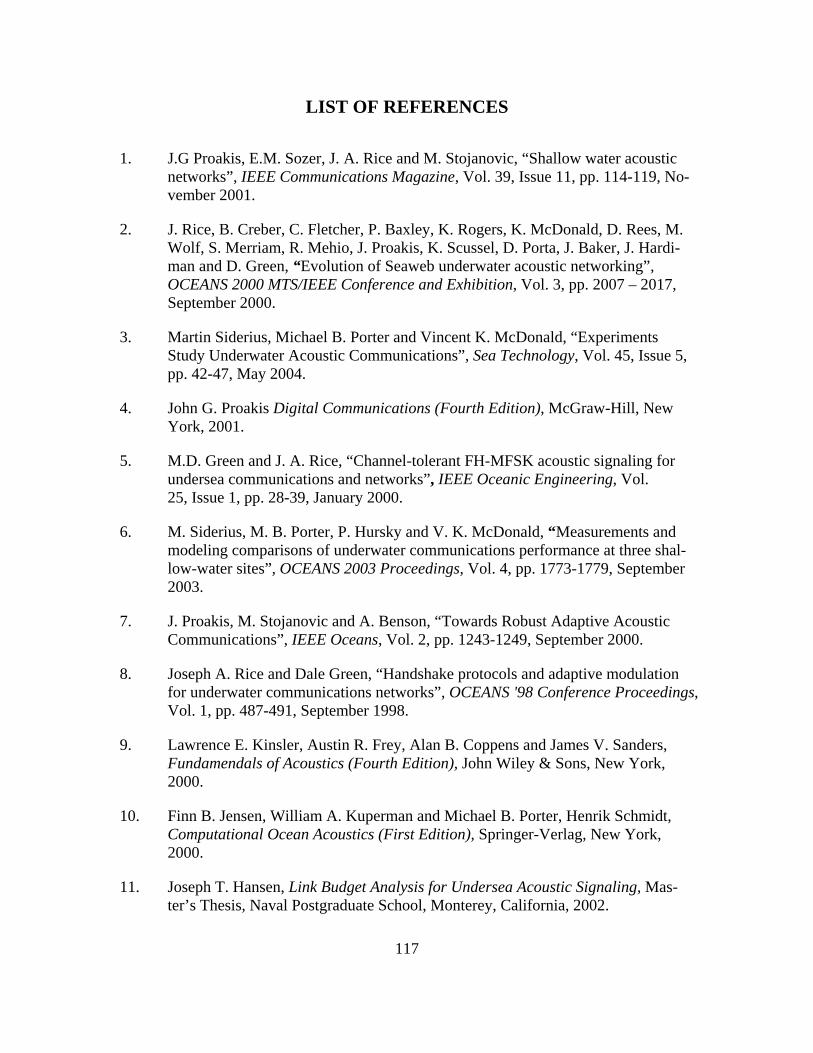
117
LIST OF REFERENCES
1. J.G Proakis, E.M. Sozer, J. A. Rice and M. Stojanovic, “Shallow water acoustic networks”, IEEE Communications Magazine, Vol. 39, Issue 11, pp. 114-119, No-vember 2001.
2. J. Rice, B. Creber, C. Fletcher, P. Baxley, K. Rogers, K. McDonald, D. Rees, M. Wolf, S. Merriam, R. Mehio, J. Proakis, K. Scussel, D. Porta, J. Baker, J. Hardi-man and D. Green, “Evolution of Seaweb underwater acoustic networking”, OCEANS 2000 MTS/IEEE Conference and Exhibition, Vol. 3, pp. 2007 – 2017, September 2000.
3. Martin Siderius, Michael B. Porter and Vincent K. McDonald, “Experiments Study Underwater Acoustic Communications”, Sea Technology, Vol. 45, Issue 5, pp. 42-47, May 2004.
4. John G. Proakis Digital Communications (Fourth Edition), McGraw-Hill, New York, 2001.
5. M.D. Green and J. A. Rice, “Channel-tolerant FH-MFSK acoustic signaling for undersea communications and networks”, IEEE Oceanic Engineering, Vol. 25, Issue 1, pp. 28-39, January 2000.
6. M. Siderius, M. B. Porter, P. Hursky and V. K. McDonald, “Measurements and modeling comparisons of underwater communications performance at three shal-low-water sites”, OCEANS 2003 Proceedings, Vol. 4, pp. 1773-1779, September 2003.
7. J. Proakis, M. Stojanovic and A. Benson, “Towards Robust Adaptive Acoustic Communications”, IEEE Oceans, Vol. 2, pp. 1243-1249, September 2000.
8. Joseph A. Rice and Dale Green, “Handshake protocols and adaptive modulation for underwater communications networks”, OCEANS '98 Conference Proceedings, Vol. 1, pp. 487-491, September 1998.
9. Lawrence E. Kinsler, Austin R. Frey, Alan B. Coppens and James V. Sanders, Fundamendals of Acoustics (Fourth Edition), John Wiley & Sons, New York, 2000.
10. Finn B. Jensen, William A. Kuperman and Michael B. Porter, Henrik Schmidt, Computational Ocean Acoustics (First Edition), Springer-Verlag, New York, 2000.
11. Joseph T. Hansen, Link Budget Analysis for Undersea Acoustic Signaling, Mas-ter’s Thesis, Naval Postgraduate School, Monterey, California, 2002.
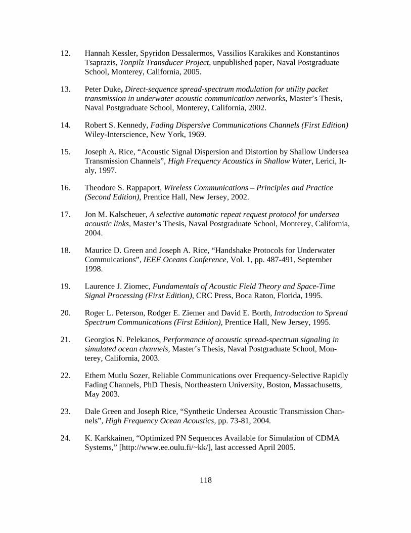
118
12. Hannah Kessler, Spyridon Dessalermos, Vassilios Karakikes and Konstantinos Tsaprazis, Tonpilz Transducer Project, unpublished paper, Naval Postgraduate School, Monterey, California, 2005.
13. Peter Duke, Direct-sequence spread-spectrum modulation for utility packet transmission in underwater acoustic communication networks, Master’s Thesis, Naval Postgraduate School, Monterey, California, 2002.
14. Robert S. Kennedy, Fading Dispersive Communications Channels (First Edition) Wiley-Interscience, New York, 1969.
15. Joseph A. Rice, “Acoustic Signal Dispersion and Distortion by Shallow Undersea Transmission Channels”, High Frequency Acoustics in Shallow Water, Lerici, It-aly, 1997.
16. Theodore S. Rappaport, Wireless Communications – Principles and Practice (Second Edition), Prentice Hall, New Jersey, 2002.
17. Jon M. Kalscheuer, A selective automatic repeat request protocol for undersea acoustic links, Master’s Thesis, Naval Postgraduate School, Monterey, California, 2004.
18. Maurice D. Green and Joseph A. Rice, “Handshake Protocols for Underwater Commuications”, IEEE Oceans Conference, Vol. 1, pp. 487-491, September 1998.
19. Laurence J. Ziomec, Fundamentals of Acoustic Field Theory and Space-Time Signal Processing (First Edition), CRC Press, Boca Raton, Florida, 1995.
20. Roger L. Peterson, Rodger E. Ziemer and David E. Borth, Introduction to Spread Spectrum Communications (First Edition), Prentice Hall, New Jersey, 1995.
21. Georgios N. Pelekanos, Performance of acoustic spread-spectrum signaling in simulated ocean channels, Master’s Thesis, Naval Postgraduate School, Mon-terey, California, 2003.
22. Ethem Mutlu Sozer, Reliable Communications over Frequency-Selective Rapidly Fading Channels, PhD Thesis, Northeastern University, Boston, Massachusetts, May 2003.
23. Dale Green and Joseph Rice, “Synthetic Undersea Acoustic Transmission Chan-nels”, High Frequency Ocean Acoustics, pp. 73-81, 2004.
24. K. Karkkainen, “Optimized PN Sequences Available for Simulation of CDMA Systems,” [http://www.ee.oulu.fi/~kk/], last accessed April 2005.

119
25. Peyton Z. Peebles, Probability, Random Variables and Random Signal Principles (Fourth Edition), McGraw-Hill Higher Education, New York, 2001.
26. Daniel Codiga, Joseph Rice and Paul Baxley, “Networked Acoustic Modems for Real-Time Data Delivery from Distributed Subsurface Instruments in the Coastal Ocean: Initial System Development and Performance”, Journal of Atmospheric and Oceanic Technology, Vol. 21, No. 2, pp. 331–346, 2004.
27. Michael B. Porter, Vincent K. McDonald, Paul A. Baxley and Joseph A. Rice, “SignalEx: Linking Environmental Acoustics with the Signaling Schemes”, IEEE, Vol. 1, pp. 595-600, September 2000.
28. David Porta, Joseph Rice and Dan Codiga, “Acoustic Modem Multi-access Net-working for Data Acquisition”, Sea Technology, Vol. 42, Issue 5, pp. 10-14, May 2001.
29. V.K. McDonald, J. A. Rice and C. L. Fletcher, “An underwater communication testbed for telesonar RDT&E”, OCEANS '98 Conference Proceedings, Vol. 2, pp. 639-643, September 1998.
30. SignalEx web site, http://hlsresearch.com/signalex (password protected), last ac-cessed April 2005.
31. Paul Hursky, Michael B. Porter and Martin Siderius, “High-frequency (8-16 KHZ) Model-based Source Localization”, Journal of the Acoustical Society of America, Vol. 115, issue 6, pp. 3021-3032, 2004.
32. BELLHOP ray/beam model web site, http://www.hlsresearch.com/oalib/Modes/ AcousticsToolbox/manual_html/node60.html, last accessed May 2005.
33. Delphi Communication Systems, Underwater Acoustic Communications Channel and Network Optimization, Technical Report, Maynard, 1999-2000.
34. F. Blackmon, E. Sozer, M. Stojanovic and J. Proakis, “Performance Comparison of RAKE and Hypothesis Feedback Direct Spread Spectrum Techniques for Un-derwater Communications Applications”, MTS/IEEE Oceans '02 Conference, Vol. 1, pp. 594-603, October 2002.
35. M. Stojanovic, J. G. Proakis, James B. Bowlin and J. A. Catiprovic, “Performance of a high-rate communication link on a shallow water acoustic channel”, Journal of the Acoustical Society of America, Vol. 95, Issue 5, pp. 2809-2810, 1994.
36. F. Blackmon, E. Sozer and J. Proakis, “Iterative Equalization, Decoding, and Soft Diversity Combining for Underwater Acoustic Channels”, MTS/IEEE Oceans '02 Conference, Vol. 4, pp. 2425-2428, October 2002.

120
THIS PAGE INTENTIONALLY LEFT BLANK

121
INITIAL DISTRIBUTION LIST
1. Defense Technical Information Center Ft. Belvoir, Virginia
2. Dudley Knox Library
Naval Postgraduate School Monterey, California
3. Chairman, Code EC/Po
Department of Electrical and Computing Engineering Naval Postgraduate School Monterey, California
4. Chairman, Code PH/Lj
Department of Physics Naval Postgraduate School Monterey, California
5. Professor Joseph Rice
Department of Physics1 Naval Postgraduate School Monterey, California
6. Professor Roberto Cristi, Code EC/Cx
Department of Electrical and Computing Engineering Naval Postgraduate School Monterey, California
7. Embassy of Greece, Naval Attaché
Washington, DC
8. Paul Baxley SPAWAR Systems Center San Diego, California
9. Allen Moshfegh
Defense Advanced Research Projects Agency (DARPA) Arlington, Virginia
10. Thomas F. Swean
Office of Naval Research Arlington, Virginia

122
11. Spyridon Dessalermos Markou Botsari 18 Lykovrisi Attikis, 14123 GREECE


