

NAVAL
POSTGRADUATE SCHOOL
MONTEREY, CALIFORNIA
THESIS
Approved for public release; distribution is unlimited
PORTABLE SIGNALS ANALYSIS SOLUTIONS USING SIGNALWORKS®: A PROCESS GUIDE FOR ANALYSTS
AND STUDENTS
by
Eric W. Sears
September 2009
Thesis Co-Advisor: Tri Ha Thesis Co-Advisor: Vicente Garcia
Second Reader: Raymond Elliott

i
REPORT DOCUMENTATION PAGE Form Approved OMB No. 0704-0188 Public reporting burden for this collection of information is estimated to average 1 hour per response, including the time for reviewing instruction, searching existing data sources, gathering and maintaining the data needed, and completing and reviewing the collection of information. Send comments regarding this burden estimate or any other aspect of this collection of information, including suggestions for reducing this burden, to Washington headquarters Services, Directorate for Information Operations and Reports, 1215 Jefferson Davis Highway, Suite 1204, Arlington, VA 22202-4302, and to the Office of Management and Budget, Paperwork Reduction Project (0704-0188) Washington DC 20503. 1. AGENCY USE ONLY (Leave blank)
2. REPORT DATE September 2009
3. REPORT TYPE AND DATES COVERED Master’s Thesis
4. TITLE AND SUBTITLE Portable Signals Analysis Solutions using Signalworks®: A Process Guide for Analysts and Students 6. AUTHOR(S) LT Eric Sears
5. FUNDING NUMBERS
7. PERFORMING ORGANIZATION NAME(S) AND ADDRESS(ES) Naval Postgraduate School Monterey, CA 93943-5000
8. PERFORMING ORGANIZATION REPORT NUMBER
9. SPONSORING /MONITORING AGENCY NAME(S) AND ADDRESS(ES) N/A
10. SPONSORING/MONITORING AGENCY REPORT NUMBER
11. SUPPLEMENTARY NOTES The views expressed in this thesis are those of the author and do not reflect the official policy or position of the Department of Defense or the U.S. Government. 12a. DISTRIBUTION / AVAILABILITY STATEMENT Approved for public release; distribution is unlimited.
12b. DISTRIBUTION CODE
13. ABSTRACT (maximum 200 words) Signalworks® is a signals analysis software suite designed to be installed on Windows and Linux
portable computing platforms. The demodulation applications within the program offer considerable processing capability for a variety of signals coupled with a graphical interface that is both easy to use and configure. This thesis examines the process of building test signals within Signalworks® and then processing them with the available demodulation applications to define important parameters used to identify and analyze signals. Although Signalworks® version 4.0 is unable to demodulate Orthogonal Frequency Division Multiplexed (OFDM) signals often used in wireless communications, it can process Binary Phase-Shift Keyed (BPSK) and Quadrature Phase-Shift Keyed (QPSK) signals used in the 802.11b standard. While future versions may include OFDM demodulation capability, this analysis includes the feasibility of using Signalworks® in a lab environment to demonstrate and educate students on signal characteristics including wireless communication signals.
15. NUMBER OF PAGES
125
14. SUBJECT TERMS Signals analysis, portable signal processing, Signalworks®
16. PRICE CODE
17. SECURITY CLASSIFICATION OF REPORT
Unclassified
18. SECURITY CLASSIFICATION OF THIS PAGE
Unclassified
19. SECURITY CLASSIFICATION OF ABSTRACT
Unclassified
20. LIMITATION OF ABSTRACT
UU NSN 7540-01-280-5500 Standard Form 298 (Rev. 8-98) Prescribed by ANSI Std. Z39.18

ii
THIS PAGE INTENTIONALLY LEFT BLANK

iii
Approved for public release; distribution is unlimited.
PORTABLE SIGNALS ANALYSIS SOLUTIONS USING SIGNALWORKS®: A PROCESS GUIDE FOR ANALYSTS AND STUDENTS
Eric W. Sears
Lieutenant, United States Navy B.S., Hawaii Pacific University, 1998
Submitted in partial fulfillment of the requirements for the degree of
MASTER OF SCIENCE IN INFORMATION WARFARE SYSTEMS ENGINEERING
from the
NAVAL POSTGRADUATE SCHOOL September 2009
Author: Eric W. Sears
Approved by: Tri Ha Thesis Co-Advisor Vicente Garcia Thesis Co-Advisor
Raymond Elliott Second Reader
Dan Boger Chairman, Department of Information Sciences

iv
THIS PAGE INTENTIONALLY LEFT BLANK

v
ABSTRACT
Signalworks® is a signals analysis software suite designed to be installed
on Windows and Linux portable computing platforms. The demodulation
applications within the program offer considerable processing capability for a
variety of signals coupled with a graphical interface that is both easy to use and
configure. This thesis examines the process of building test signals within
Signalworks®, and then processing them with the available demodulation
applications to define important parameters used to identify and analyze signals.
Although Signalworks® version 4.0 is unable to demodulate Orthogonal
Frequency Division Multiplexed (OFDM) signals often used in wireless
communications, it can process Binary Phase-Shift Keyed (BPSK) and
Quadrature Phase-Shift Keyed (QPSK) signals used in the 802.11b standard.
While future versions may include OFDM demodulation capability, this analysis
includes the feasibility of using Signalworks® in a lab environment to
demonstrate and educate students on signal characteristics including wireless
communication signals.

vi
THIS PAGE INTENTIONALLY LEFT BLANK

vii
TABLE OF CONTENTS
I. INTRODUCTION............................................................................................. 1 A. OVERVIEW OF SIGNALWORKS® SOFTWARE SUITE .................... 1 B. OBJECTIVE ......................................................................................... 2 C. THESIS ORGANIZATION.................................................................... 2
II. PHASE-SHIFT KEYED SIGNAL ANALYSIS ................................................. 5 A. OVERVIEW OF PHASE-SHIFT KEYED SIGNALS ............................. 5
1. Signal Characteristics ............................................................. 5 2. Applications ............................................................................. 6
B. GENERATING TEST SIGNAL WITH SIGNALGEN............................. 7 1. Procedural Guidance............................................................... 7 2. Creating a BPSK Signal using the Signalworks®
SignalGen Application ............................................................ 7 C. INITIAL ANALYSIS WITH PREVIEW ................................................ 15
1. Procedural Guidance............................................................. 15 2. Initial Analysis using the Signalworks® Preview
Application ............................................................................. 16 D. ADDITIONAL ANALYSIS WITH DEMOD.......................................... 23
1. Procedural Guidance............................................................. 23 2. Advanced Analysis with Demod........................................... 23
E. BPSK ANALYSIS RESULTS............................................................. 24
III. QUADRATURE PHASE-SHIFT KEYED SIGNAL ANALYSIS ..................... 27 A. OVERVIEW OF QUADRATURE PHASE-SHIFT KEYED SIGNALS. 27
1. Signal Characteristics ........................................................... 27 2. Applications ........................................................................... 28
B. GENERATING QPSK TEST SIGNAL WITH SIGNALGEN ............... 28 1. Procedural Guidance............................................................. 28 2. Creating a QPSK Signal using the Signalworks®
SignalGen Application .......................................................... 28 C. INITIAL ANALYSIS WITH PREVIEW ................................................ 32
1. Procedural Guidance............................................................. 32 2. Initial Analysis using the Signalworks® Preview
Application ............................................................................. 33 D. ADDITIONAL ANALYSIS WITH DEMOD.......................................... 40
1. Procedural Guidance............................................................. 40 2. Advanced Analysis with Signalworks’® Demod
Application ............................................................................. 40 E. QPSK ANALYSIS RESULTS ............................................................ 43
IV. QUADRATURE AMPLITUDE MODULATION SIGNAL ANALYSIS ............ 45 A. OVERVIEW OF QUADRATURE AMPLITUDE MODULATION
SIGNALS ........................................................................................... 45 1. Signal Characteristics ........................................................... 45

viii
2. Applications ........................................................................... 46 B. GENERATING QAM TEST SIGNAL WITH SIGNALGEN ................. 46
1. Procedural Guidance............................................................. 46 2. Creating a QAM Signal using the Signalworks®
SignalGen Application .......................................................... 47 C. INITIAL QAM ANALYSIS WITH PREVIEW....................................... 51
1. Procedural Guidance............................................................. 51 2. Initial QAM Analysis using the Signalworks® Preview
Application ............................................................................. 52 D. ADDITIONAL QAM ANALYSIS WITH DEMOD ................................ 59
1. Procedural Guidance............................................................. 59 2 Advanced QAM Analysis with the Signalworks® Demod
Application ............................................................................. 59 E. WORKING WITH ADVANCED QAM SIGNALS ................................ 63
1. Beyond 8-State QAM ............................................................. 63 2. Generating 16-State QAM with Signalworks®..................... 63 3. Generating 64-State QAM with Signalworks®..................... 64 4. Initial analysis of 16-State QAM with Preview ..................... 65 5. Initial Analysis of 64-State QAM with Preview .................... 69 6. Advanced Analysis of 16-State QAM with Demod .............. 73 7. Advanced Analysis of 64-State QAM with Demod .............. 76
F. QAM ANALYSIS RESULTS .............................................................. 79
V. WI-FI SIGNAL ANALYSIS............................................................................ 81 A. OVERVIEW OF WIFI SIGNALS......................................................... 81
1. Signal Characteristics ........................................................... 81 2. Application ............................................................................. 81
B. INITIAL ANALYSIS WITH PREVIEW ................................................ 81 1. Procedural Guidance............................................................. 81 2. Initial Analysis using the Signalworks® Preview
Application ............................................................................. 82 C. ADDITIONAL WIFI ANALYSIS WITH DEMOD ................................. 90
1. Procedural Guidance............................................................. 90 2. Advanced Analysis with the Signalworks® Demod
Application ............................................................................. 91 D. WIFI ANALYSIS RESULTS ............................................................. 100
VI. SUMMARY AND RECOMMENDATIONS FOR FUTURE WORK................ 101 A. SUMMARY....................................................................................... 101
1. Installation and Operation................................................... 101 2. Capabilities and Limitations ............................................... 102 3. Findings................................................................................ 102
B. RECOMMENDATIONS FOR FUTURE WORK................................ 103
LIST OF REFERENCES........................................................................................ 105
INITIAL DISTRIBUTION LIST ............................................................................... 107
ix
LIST OF FIGURES
Figure 1. BPSK waveform ................................................................................... 5 Figure 2. BPSK polar plot .................................................................................... 6 Figure 3. Recall default parameters window........................................................ 7 Figure 4. Input bit operations editor ..................................................................... 8 Figure 5. SignalGen for BPSK procedures .......................................................... 8 Figure 6. Raised cosine, 0 (Nyquist minimum bandwidth) ........................... 10 Figure 7. Raised cosine, .5 ......................................................................... 11 Figure 8. Raised cosine, 1 ........................................................................... 12 Figure 9. SignalGen modulation window for BPSK............................................ 13 Figure 10. Carrier frequency default .................................................................... 13 Figure 11. Carrier frequency set to 1700 KHz ..................................................... 13 Figure 12. SignalGen test point at Baseband Modulation output......................... 14 Figure 13. BPSK Baseband Modulated test point display ................................... 15 Figure 14. BPSK Preview window ....................................................................... 16 Figure 15. BPSK File input selection ................................................................... 17 Figure 16. BPSK Preview test point at file input .................................................. 17 Figure 17. BPSK Preview test point display ........................................................ 18 Figure 18. BPSK Preview band center specified ................................................. 19 Figure 19. BPSK Preview test point at Center Freq. Detector ............................. 19 Figure 20. BPSK center frequency marker .......................................................... 20 Figure 21. BPSK baud rate display...................................................................... 21 Figure 22. BPSK export/save for Demod............................................................. 22 Figure 23. BPSK Demod test point at mixer output ............................................. 23 Figure 24. BPSK Demod test point display.......................................................... 24 Figure 25. QPSK polar plot.................................................................................. 27 Figure 26. QPSK Recall default parameters window........................................... 29 Figure 27. Input Bit Operations Editor ................................................................. 29 Figure 28. SignalGen for QPSK procedures........................................................ 30 Figure 29. SignalGen Modulation window for QPSK ........................................... 30 Figure 30. Carrier frequency set to 3000 KHz ..................................................... 31 Figure 31. SignalGen test point at Baseband Modulation output......................... 31 Figure 32. QPSK Baseband Modulation test point display .................................. 32 Figure 33. QPSK Preview window....................................................................... 33 Figure 34. QPSK file input selection .................................................................... 34 Figure 35. QPSK Preview test point at file input .................................................. 34 Figure 36. QPSK Preview test point display ........................................................ 35 Figure 37. QPSK Preview band center................................................................ 36 Figure 38. QPSK Preview test point at Center Frequency Detector .................... 36 Figure 39. QPSK center frequency marker.......................................................... 37 Figure 40. QPSK baud rate display ..................................................................... 38 Figure 41. QPSK export/save for Demod ............................................................ 39 Figure 42. QPSK Demod test point at mixer output............................................. 40

x
Figure 43. QPSK Demod test point display with poor grouping........................... 41 Figure 44. QPSK PSK demodulator .................................................................... 42 Figure 45. QPSK Demod test point display with optimal grouping....................... 43 Figure 46. 8 level QAM polar plot ........................................................................ 45 Figure 47. Recall default parameters window...................................................... 47 Figure 48. Input Bit Operations Editor ................................................................. 48 Figure 49. SignalGen for QAM procedures ......................................................... 48 Figure 50. SignalGen Modulation window for QAM............................................. 49 Figure 51. Carrier frequency set to 2750 KHz ..................................................... 49 Figure 52. SignalGen test point of Baseband Modulation output......................... 50 Figure 53. QAM Baseband Modulation test point display .................................... 51 Figure 54. QAM Preview window......................................................................... 52 Figure 55. QAM file input selection...................................................................... 53 Figure 56. QAM Preview test point at file input.................................................... 53 Figure 57. QAM Preview test point display.......................................................... 54 Figure 58. QAM Preview band center specification ............................................. 55 Figure 59. QAM Preview test point at Center Frequency Detector ...................... 55 Figure 60. QAM center frequency marker ........................................................... 56 Figure 61. QAM baud rate display ....................................................................... 57 Figure 62. QAM export/save for Demod .............................................................. 58 Figure 63. QAM Demod test point at mixer output............................................... 59 Figure 64. QAM Demod test point display with poor groupings ........................... 60 Figure 65. QAM Demod PSK Demodulator window ............................................ 61 Figure 66. QAM Demod test point display with acceptable groupings................. 62 Figure 67. 16-State QAM SignalGen modulation window.................................... 63 Figure 68. 16-State QAM Carrier frequency set to 2000 KHz.............................. 64 Figure 69. 64-State QAM SignalGen modulation window.................................... 65 Figure 70. 64-State QAM Carrier frequency set to 2,600 KHz............................. 65 Figure 71. 16-State QAM Preview test point for double squared center
frequency............................................................................................ 66 Figure 72. 16-State QAM test point display for double carrier frequency ............ 67 Figure 73. 16-State QAM baud rate display ........................................................ 68 Figure 74. 16-State QAM export/save for Demod window................................... 69 Figure 75. 16-State QAM test point for double frequency squaring ..................... 70 Figure 76. 16-State QAM center frequency display ............................................. 71 Figure 77. 16-State QAM baud rate display ........................................................ 72 Figure 78. 16-State QAM export/save for Demod................................................ 73 Figure 79. 16 State QAM Demod with mixer test point selected.......................... 73 Figure 80. 16-State QAM mixer test point display with poor grouping ................. 74 Figure 81. 16-State QAM Demod PSK Demodulator window.............................. 75 Figure 82. 16-State QAM mixer test point display with acceptable grouping....... 76 Figure 83. 64-State QAM Demod with mixer test point selected ......................... 77 Figure 84. 64-State QAM mixer test point display with poor grouping ................. 77 Figure 85. 64-State QAM Demod PSK Demodulator window.............................. 78 Figure 86. 64-State QAM mixer test point display with acceptable grouping....... 79

xi
Figure 87. Recall window .................................................................................... 82 Figure 88. Start and Stop control buttons ............................................................ 83 Figure 89. Test point display, Preview, and File Input window screen
configuration....................................................................................... 83 Figure 90. Filter Setup for wifi1.wrd ..................................................................... 85 Figure 91. Center frequency measurement for wifi1.wrd ..................................... 86 Figure 92. Baudrate detector display with 11Mb/s wifi1.wrd signal...................... 87 Figure 93. Inaccurate center frequency depicted in I&Q test point display .......... 88 Figure 94. IQ display with adjusted frequency..................................................... 89 Figure 95. Export/Save for Demod window ......................................................... 90 Figure 96. Mixer test point display of wifi1.wrd in Demod.................................... 91 Figure 97. Bit Operations display for wifi1.wrd..................................................... 92 Figure 98. Bit Operations Editor with Keep/Skip tool with expanded functions.... 93 Figure 99. Search and Scan window with LRS tab selected ............................... 94 Figure 100. LRS Scan Correlation with single spike.............................................. 95 Figure 101. Search and Scan window with populated Results .............................. 96 Figure 102. Bit Operations Editor with LRS Decode tool applied........................... 97 Figure 103. Bit Output display with 48 bit frame size............................................. 98 Figure 104. Bit Output with 0-F Hex display .......................................................... 99 Figure 105. HEX display with highlighted MAC addresses.................................. 100

xii
THIS PAGE INTENTIONALLY LEFT BLANK

xiii
LIST OF ACRONYMS AND ABBREVIATIONS
AGC Automatic gain control
BPSK Binary Phase-Shift Keyed
EW Electronic Warfare
FSK Frequency Shift Keyed
GMSK Gaussian=Minimum Shift Keyed
LRS Linear Recursive Sequence
MB/s Megabits per second
MSK Minimum-Shift Keyed
OFDM Orthogonal Frequency Division Multiplexed
PSK Phase-Shift Keyed
QAM Quadrature Amplitude Modulation
QPSK Quadrature Phase-Shift Keyed
RF Radio Frequency
RFID Radio Frequency Identification
WLAN Wireless Local Area Network
WMAN Wireless Metropolitan Area Network

xiv
THIS PAGE INTENTIONALLY LEFT BLANK

xv
ACKNOWLEDGMENTS
I thank my wife, children, and extended family for enduring countless
hours of my absence while I was completing this project. They are the
foundation of my success in the Navy and are most deserving of recognition.
Their love and support through this and previous tours is the wind in my sails. I
also thank Professor Tri Ha for his determination and guidance as my advisor.
His background in signals and signal theory is extensive, and has proven critical
to my research. Additionally, I thank Professor Vicente Garcia, whom I sought
out as a fellow Cryptologist in search of research assistance. Although retired,
he is a staunch advocate for our community and continues to serve us well. The
staff at Signami-DCS were outstanding in their support. I specifically wish to
thank Mr. Terry Cutshaw, Mr. Jacob Rorick, and Mr. Gary Kenworthy for their
guidance and technical assistance.

xvi
THIS PAGE INTENTIONALLY LEFT BLANK

1
I. INTRODUCTION
A. OVERVIEW OF SIGNALWORKS® SOFTWARE SUITE
The Signalworks® software package developed by Signami-DCS is a
Windows or Linux based suite of software tools that incorporates complex
algorithms to enable advanced signals analysis. When coupled to a digital input,
Signalworks® offers all the advantages of typical analysis equipment such as
digital oscilloscopes, spectrum analyzers, and demodulators, combined into a
simple to use interface requiring no programming or coding. Input to
Signalworks® is accomplished via prerecorded files or through a digitizing
component directly input to the computer. Signalworks® is capable of
processing a variety of signal formats including Phase-Shift Keyed (PSK),
Quadrature Amplitude Modulation (QAM), Frequency-Shift Keyed (FSK),
Minimum-Shift Keyed (MSK), and Gaussian Minimum-Shift Keyed (GMSK).
Signalworks® can breakout carrier frequency, symbol rate, modulation type, bit
encoding and framing, and conduct link analysis to determine bit error rate and
causes for performance degradation. Signalworks® is designed to be installed
and operated on a Windows or Linux portable computer with minimal processing
and memory requirements.
The software suite is divided into three main applications: Preview,
Demod, and SignalGen. Preview is the analyst’s initial step to define basic
parameters and apply filters to enable the demodulator to process the signal.
Preview allows the analyst to set an arbitrary center frequency, bandwidth, or
roll-off frequency. The carrier frequency can be determined within Preview
through second, fourth, and eighth order algorithms. The baud rate is also
defined with the Preview application. Once these basic parameters have been
determined, the analyst can view the results within Preview through a variety of
time and frequency displays. Demod is the Signalworks® demodulator and
equalizer. Within Demod, the analyst can select the signal format, choosing from
PSK, QAM, FSK, MSK, and GMSK. Equalization can be adjusted by selecting
2
line canceling, dispersion-direction, or direction-detection algorithms. The
analyst can utilize Demod to conduct bit-level analysis such as decoding,
remapping, and frame sync operations. As with Preview, Demod offers the
analyst a variety of display options both in time and frequency domains. Data
displayed can be raw, intermediate, or processed signal externals. Demod can
process teleprinter traffic in real-time and produce text outputs.
SignalGen allows the user analyst to generate their own signals with bit
files or linear recursive sequencing pseudo-random noise generators. Signals
can be simulated with varying sample and modulation rates having raised cosine
or root raised cosine pulse shapes. Simulations include adding noise with
arbitrary noise signal-to-noise ratios. Bit level operations are available for
encoding and remapping. Once signals are generated, they are saved in an
output file for later use in Preview or Demod.
B. OBJECTIVE
The objective of this thesis was to document the procedures for
generating various signal formats and then processing them using Signalworks®
for use in lab environments. While Signalworks® cannot yet demodulate
Orthogonal Frequency Division Multiplexed (OFDM) signals used in wireless
communications, it already offers considerable ability to process a variety of
complex signals. An additional part of this project is to provide a feasibility study
on whether Signalworks® is a viable platform to use in student labs to
demonstrate signal characteristics, including wireless communication signals
such as the 802.16 IEEE standard of signals.
C. THESIS ORGANIZATION
This thesis details how a user would build a signal and then process it to
measure various parameters and determine the modulation within the
Signalworks® software suite. The intended use of this detailed procedure is to
include it as part of a class and lab curriculum. The thesis is organized into the
following chapters:
3
Chapter II focuses on Phase-shift keyed signals. An initial overview of
PSK signals and their typical applications is followed by a detailed systematic
procedure from building a simulated PSK signal to inputting this simulated signal
into Signalworks® for processing.
Chapter III covers Quadrature Phase-shift keyed signals. An initial
overview of PSK signals and their typical applications is followed by a detailed
systematic procedure from building a simulated QPSK signal to inputting this
simulated signal into Signalworks® for processing.
Chapter IV contains information on Quadrature Amplitude Modulated
signals to include 8, 16, and 64 State QAM signal formats. An initial overview of
QAM signals and their typical applications is followed by a detailed systematic
procedure from building a simulated QAM signal to inputting this simulated signal
into Signalworks® for processing.
Chapter V focuses on wireless communication signals. Although
Signalworks® has limited capability to process wireless communication signals, it
allows signals to be viewed even if demodulation is not possible. .A general
procedure for future use also is defined.
Chapter VI provides conclusions and recommendations.
This chapter provided background to the Signalworks® software suite and
justification for the need of this project.

4
THIS PAGE INTENTIONALLY LEFT BLANK

5
II. PHASE-SHIFT KEYED SIGNAL ANALYSIS
A. OVERVIEW OF PHASE-SHIFT KEYED SIGNALS
1. Signal Characteristics
Phase-shift keying (PSK) is a product of the space program. PSK is a
digital modulation technique that transmits data by changing the phase of the
carrier frequency. The mathematical expression used for PSK is
0
2( ) cos[ ]i i
Es t t
T
0
1,...,
t T
i M
The phase term i will have M discrete values (Sklar 1079). The receiver in a
phase-modulated system must have a reference oscillator to compare the
incoming signal and determine if it is in-phase or if not, determine the relative
phase compared to the reference. This section focuses on a binary signal having
two transmitted phases, 180° apart. In binary phase-shift keyed (BPSK) signals,
the frequency waveform utilizes one phase to convey a one and another phase
to convey a zero as depicted in the diagram below (Sklar 1079).
Figure 1. BPSK waveform
On a polar plot, a BPSK signal is depicted as vectors, with the vector
length corresponding to the signal amplitude and the vector direction

6
corresponding to the phase relative to each signal in the set. In a BPSK, M = 2
so there are two vectors separated by 180° on the plot. The diagram below
depicts a BPSK polar plot.
Figure 2. BPSK polar plot
2. Applications
PSK modulation is relatively simple in theory and operation. Because of
this simplicity, it is widely used in a variety of applications. As mentioned
previously, BPSK was first utilized in space applications. Its use was prominent
in early digital broadcast satellite television systems, mainly in low-power satellite
applications (Van der Wal and Montreuil 30-41). The simplicity of a PSK signal
makes it an ideal modulation technique for low-cost passive transmitters such as
Radio Frequency Identification (RFID) devices. RFID implementations range
from asset tracking to credit cards to biometric passports. The basic IEEE
802.11b standard utilizes BPSK modulation, although only for slow data rate
systems.

7
B. GENERATING TEST SIGNAL WITH SIGNALGEN
1. Procedural Guidance
This portion of the thesis begins the systematic procedures defining how
to use the signal generation capabilities of Signalworks® with BPSK signals. To
create and save signals within Signalworks®, the SignalGen application will be
used. The following steps detail how to create a BPSK signal.
2. Creating a BPSK Signal using the Signalworks® SignalGen Application
To open SignalGen with default parameter settings, hold SHIFT while
double clicking the SignalGen icon, if installed on the desktop, or select “All
Programs>Signalworks>SignalGen.” The first window that appears allows users
to recall normal parameter settings, user defined settings, or default settings.
Select “Cancel” to use default settings.
Figure 3. Recall default parameters window
Close the “Tip of the Day.” The SignalGen window is now displayed.
Click on the “Bit Operations” button. A new window pops up showing various tool
palette input operations. For now, drag and drop the “LRS Encode” tool into the
right-hand side of the window in the “Applied Operations” space. Click “OK.”

8
Figure 4. Input bit operations editor
Click on the “Signal” button underneath the baseband operations label in
the SignalGen window.
Figure 5. SignalGen for BPSK procedures
The SignalGen Modulation window pops up. Select “PSK” on the left
hand side of the window.
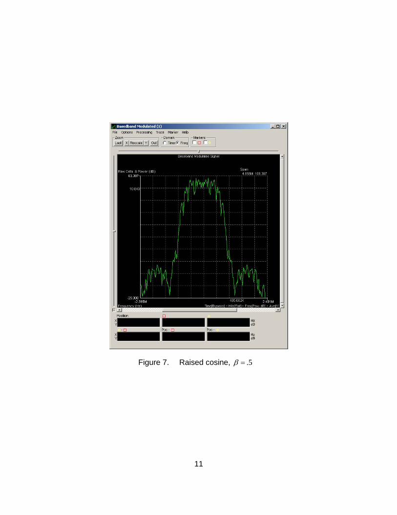
Before closing this window, notice the pulse shaping pull down menu. The
pulse shaping default is raised-cosine with beta equal to one. Pulse shaping is

9
used to achieve bandwidth reduction with respect to a rectangular pulse. The
raised-cosine filter is the most popular pulse shape. The frequency response
can be expressed as
102
0 0
2( ) cos
4
f W WH f
W W
,
0
0
2
2
f W W
W W f W
f W
W is the absolute bandwidth and 0W = 12T is the Nyquist bandwidth for
the rectangular spectrum and the half-amplitude point for the raised-cosine
spectrum. The difference 0W W is excess bandwidth or that which is beyond
the Nyquist minimum. Roll-off factor, defined to be 0 0( ) /r W W W where
0 1r , is the excess bandwidth divided by the filter −6dB bandwidth. The roll-
off r specifies the required excess bandwidth as a fraction of 0W and
characterizes the steepness of the filter roll off. When 1r , the required excess
bandwidth is 100% and the tails of the pulse are quite small. This produces a
symbol rate of SR symbols per second using a bandwidth of SR hertz, which is
twice the Nyquist minimum bandwidth (Sklar 1079). The following figures show
the difference in the pulse shape if the roll-off factor ( ) is set to zero, one-half,
or one.

10
Figure 6. Raised cosine, 0 (Nyquist minimum bandwidth)
11
Figure 7. Raised cosine, .5

12
Figure 8. Raised cosine, 1
All other settings will remain the same and should be the same as the
default settings shown below. Click “Close.”

13
Figure 9. SignalGen modulation window for BPSK
We will now change the carrier frequency to 1.700MHz. In the SignalGen
window, select the “Carrier Frequency” button on the lower left.
Figure 10. Carrier frequency default
Figure 11. Carrier frequency set to 1700 KHz

14
Move the mouse over the arrow buttons directly under the column display
and change the entry from 2.500 to 1.700. Click “Close.”
Now the signal is ready to be viewed on a display prior to saving it for
further analysis. The unlabeled boxes in the SignalGen window are for opening
display plots. Select the display that comes after the baseband modulation box.
Figure 12. SignalGen test point at Baseband Modulation output
This will open up a blank Baseband Modulated display similar to an
oscilloscope. With both the SignalGen and the Baseband Modulated windows
within view, select the “play” button at the top left of the SignalGen window.
The display should now show a PSK signal like the one below.

15
Figure 13. BPSK Baseband Modulated test point display
Let the signal continue to play and select the “Save as…” button
underneath the Output File label on the SignalGen window. Select the desired
directory where you would like to store this custom file and ensure the extension
is .”byt.” Name the file and select “Save.” When the save is complete, you can
stop playing the PSK signal you just created. The next step is to open Preview
and begin doing the analysis on this signal. Close the SignalGen window.
C. INITIAL ANALYSIS WITH PREVIEW
1. Procedural Guidance
A test signal has just been created using SignalGen. Now that signal will
be analyzed using the Preview application within Signalworks®. The Preview
application allows us to measure some basic parameters and prepare the signal
for further analysis using the Demod application.
16
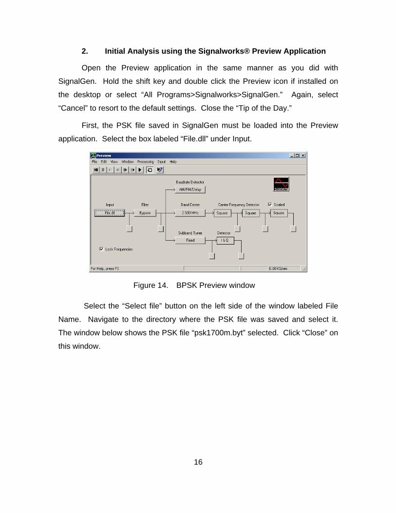
2. Initial Analysis using the Signalworks® Preview Application
Open the Preview application in the same manner as you did with
SignalGen. Hold the shift key and double click the Preview icon if installed on
the desktop or select “All Programs>Signalworks>SignalGen.” Again, select
“Cancel” to resort to the default settings. Close the “Tip of the Day.”
First, the PSK file saved in SignalGen must be loaded into the Preview
application. Select the box labeled “File.dll” under Input.
Figure 14. BPSK Preview window
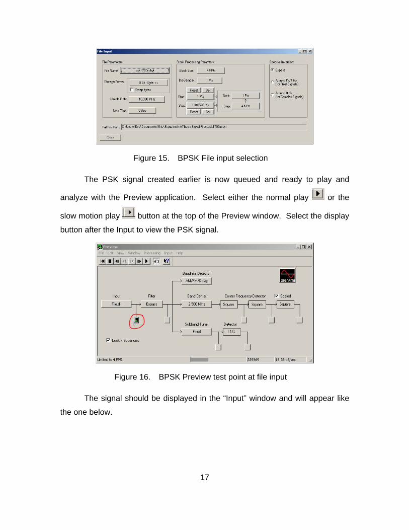
Select the “Select file” button on the left side of the window labeled File
Name. Navigate to the directory where the PSK file was saved and select it.
The window below shows the PSK file “psk1700m.byt” selected. Click “Close” on
this window.
17
Figure 15. BPSK File input selection
The PSK signal created earlier is now queued and ready to play and
analyze with the Preview application. Select either the normal play or the
slow motion play button at the top of the Preview window. Select the display
button after the Input to view the PSK signal.
Figure 16. BPSK Preview test point at file input
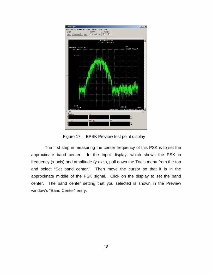
The signal should be displayed in the “Input” window and will appear like
the one below.
18
Figure 17. BPSK Preview test point display
The first step in measuring the center frequency of this PSK is to set the
approximate band center. In the Input display, which shows the PSK in
frequency (x-axis) and amplitude (y-axis), pull down the Tools menu from the top
and select “Set band center.” Then move the cursor so that it is in the
approximate middle of the PSK signal. Click on the display to set the band
center. The band center setting that you selected is shown in the Preview
window’s “Band Center” entry.
19
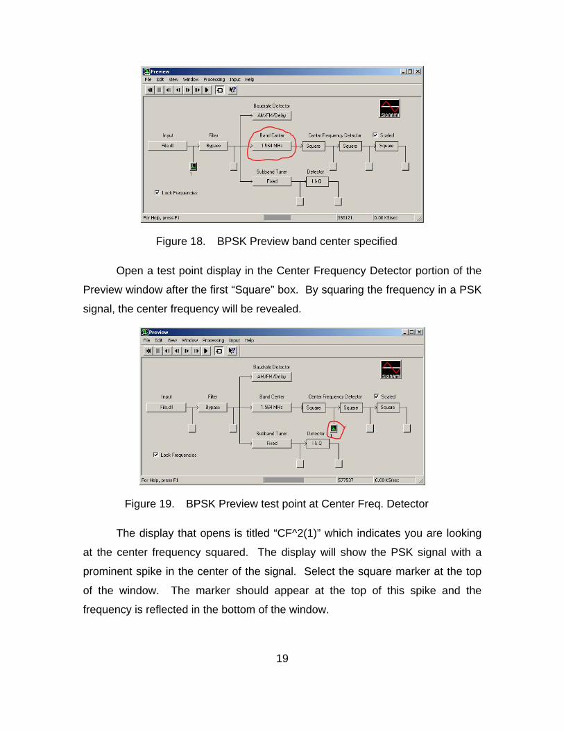
Figure 18. BPSK Preview band center specified
Open a test point display in the Center Frequency Detector portion of the
Preview window after the first “Square” box. By squaring the frequency in a PSK
signal, the center frequency will be revealed.
Figure 19. BPSK Preview test point at Center Freq. Detector
The display that opens is titled “CF^2(1)” which indicates you are looking
at the center frequency squared. The display will show the PSK signal with a
prominent spike in the center of the signal. Select the square marker at the top
of the window. The marker should appear at the top of this spike and the
frequency is reflected in the bottom of the window.

20
Figure 20. BPSK center frequency marker
The center frequency should be 1.7MHz, which corresponds to what was
defined as the carrier frequency in SignalGen when creating this signal. Leave
this window open.
Next, we will derive the symbol (baud) rate or keying rate. Assure the
PSK signal sample is playing, in either full motion or slow motion, and then select
the “AM/FM/Delay” button underneath the Baud rate label on the Preview
window. A new window will open, select the AM Detector test point to bring up a
new display.

21
Figure 21. BPSK baud rate display
Select the other marker at the top of the window and assure the marker is
placed on the left most spike within the AM Baud rate display. You can drag the
marker to the left most spike if it is not placed there automatically. The
measurement at the bottom of the display should read “1.25MHz” which is the
baud rate specified when building this signal file in SignalGen. Leave this
window open.
The center frequency (carrier) has been measured and the symbol rate,
which is also the bit rate in this case, has been measured.
22
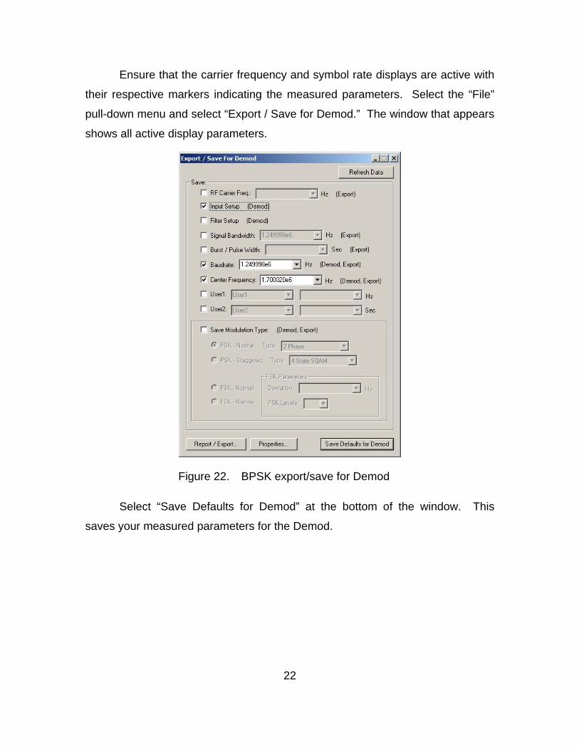
Ensure that the carrier frequency and symbol rate displays are active with
their respective markers indicating the measured parameters. Select the “File”
pull-down menu and select “Export / Save for Demod.” The window that appears
shows all active display parameters.
Figure 22. BPSK export/save for Demod
Select “Save Defaults for Demod” at the bottom of the window. This
saves your measured parameters for the Demod.

23
D. ADDITIONAL ANALYSIS WITH DEMOD
1. Procedural Guidance
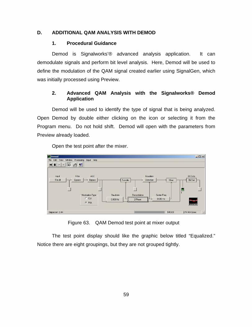
Demod is the advanced analysis feature of Signalworks®. It can
demodulate signals and perform bit-level analysis. Demod will be used to define
the modulation of the signal created earlier using SignalGen, which was initially
processed using Preview.
2. Advanced Analysis with Demod
Open Demod either by double clicking on the icon or by selecting it from
the Program menu. Do not hold shift. Demod will open with the parameters from
Preview already loaded.
Open the test point after the mixer.
Figure 23. BPSK Demod test point at mixer output
The test point display should appear similar to Figure 24 shown below with
annotations to help explain the varying phase shifts and axis labels. Notice there
are two groupings along the I axis, which appear as small dots on the display.
The display is a polar plot of a binary phased signal. These dots are two different
phase symbols, 180° apart, which represent a 1 and a 0. Although the graphic is
static, viewing the display on the computer will show that there are variations on
the grouped plot as each symbol is transmitted.

24
Figure 24. BPSK Demod test point display
If the modulation was not correctly defined, the two groupings would not
be locked into the position shown in Figure 24. Viewing this on the computer
with the incorrect modulation technique defined would result in the appearance of
a circle as the groupings spin about the center of the plot. The display in Figure
24 is the desired presentation and shows that the modulation selected is the
signal’s actual modulation. This signal is defined as a 2-State or Binary Phase-
Shift Keyed signal.
E. BPSK ANALYSIS RESULTS
This completes the BPSK portion of the project. In this section,
Signalworks® was used to generate a BPSK signal using SignalGen and then
analyze that signal using Preview and Demod. In a real-world situation, the
signal would be input to Signalworks® via a digitizer connected to the host

25
computer. The user would not know the type of signal, and thus would begin the
process of changing the modulation until the display at the end of the Demod
procedure was achieved. Once the carrier frequency and the baud rate are set,
the only change necessary is to the modulation technique. In a real-world
scenario, additional noise may also be present requiring the need for filters to
isolate the signal.

26
THIS PAGE INTENTIONALLY LEFT BLANK
27
III. QUADRATURE PHASE-SHIFT KEYED SIGNAL ANALYSIS
A. OVERVIEW OF QUADRATURE PHASE-SHIFT KEYED SIGNALS
1. Signal Characteristics
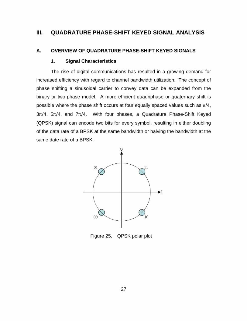
The rise of digital communications has resulted in a growing demand for
increased efficiency with regard to channel bandwidth utilization. The concept of
phase shifting a sinusoidal carrier to convey data can be expanded from the
binary or two-phase model. A more efficient quadriphase or quaternary shift is
possible where the phase shift occurs at four equally spaced values such as π/4,
3π/4, 5π/4, and 7π/4. With four phases, a Quadrature Phase-Shift Keyed
(QPSK) signal can encode two bits for every symbol, resulting in either doubling
of the data rate of a BPSK at the same bandwidth or halving the bandwidth at the
same date rate of a BPSK.
Figure 25. QPSK polar plot
28
Mathematically, a QPSK is represented as follows:
0
2( ) cos 2 1i
Es t t i
T M
0
1,...,
t T
i M
M is equal to four to reflect the four phase shifts used to represent the bit
pairs. The parameter E represents the symbol energy, and T is the symbol time.
2. Applications
Similar to BPSK modulated signals, QPSK modulation was first developed
for space applications, and eventually found its way into many types of
communications systems where spectrum conservation is necessary. Today,
more advanced signal modulation techniques dominate, but systems with limited
spectrum still utilize QPSK formats. As more points are introduced to the
constellation, the error rate increases. The balance is determined by the user,
who dictates the desired throughput for a given spectrum and either accepts a
certain level of error, or implements additional solutions to minimize error while
sustaining a certain data rate.
B. GENERATING QPSK TEST SIGNAL WITH SIGNALGEN
1. Procedural Guidance
This portion of the thesis begins the systematic procedures defining how
to use the signal generation capabilities of Signalworks® with QPSK signals. To
create and save signals within Signalworks®, the SignalGen application will be
used. The following steps detail how to create a QPSK signal.
2. Creating a QPSK Signal using the Signalworks® SignalGen Application
To open SignalGen with default parameter settings, hold SHIFT while
double clicking the SignalGen icon if installed on the desktop or select “All
Programs>Signalworks>SignalGen.” The first window that appears allows

29
users to recall normal parameter settings, user defined settings, or default
settings. Select “Cancel” to use default settings.
Figure 26. QPSK Recall default parameters window
Close the “Tip of the Day.” The SignalGen window is now displayed.
Click on the “Bit Operations” button. A new window pops up showing various tool
palette input operations. Drag and drop the “QPSK Perm” and “LRS Encode”
tools into the right-hand side of the window in the “Applied Operations” space.
Click “OK.”
Figure 27. Input Bit Operations Editor
Click on the “Signal” button underneath the baseband operations label in
the SignalGen window.

30
Figure 28. SignalGen for QPSK procedures
The SignalGen Modulation window pops up. Select “PSK” on the left
hand side of the window. Select the “2 Phase” button next to the Constellation
label and select “4 Phase.” Next, select the “2.500 Mbps” button next to Bit Rate
and change the bit rate to “3.400 Mbps.” All other settings will remain the same
and should be the same as the default settings shown below. Click “Close.”
Figure 29. SignalGen Modulation window for QPSK
We will now change the carrier frequency to 3.000MHz. In the SignalGen
window, select the “Carrier Frequency” button on the lower left. Move the mouse
over the arrow buttons directly under the column display and change the entry
from 2.500 to 3.000. Click “Close.”

31
Figure 30. Carrier frequency set to 3000 KHz
Now the signal is ready to be viewed on a display prior to saving it for
further analysis. The unlabeled boxes in the SignalGen window are for opening
display plots. Select the test point display that comes after the Baseband
Modulation box.
Figure 31. SignalGen test point at Baseband Modulation output
This will open up a blank Baseband Modulated display similar to an
oscilloscope. With both the SignalGen and the Baseband Modulated windows
within view, select the “play” button at the top left of the SignalGen window.
The display should now show a QPSK signal like the one below.

32
Figure 32. QPSK Baseband Modulation test point display
Let the signal continue to play and select the “Save as…” button
underneath the Output File label on the SignalGen window. Select the desired
directory where you would like to store this custom file and ensure the extension
is ”byt.” Name the file and select “Save.” When the save is complete, you can
stop playing the PSK signal you just created. The next step is to open Preview
and begin doing the analysis on this signal. Close the SignalGen window.
C. INITIAL ANALYSIS WITH PREVIEW
1. Procedural Guidance
A QPSK test signal has just been created using SignalGen. The signal is
ready to be analyzed using the Preview application within Signalworks®. The
Preview application allows us to measure some basic parameters and prepare
the signal for further analysis using the Demod application.
33
2. Initial Analysis using the Signalworks® Preview Application
Open the Preview application in the same manner as you did with
SignalGen. Hold the shift key and double click the Preview icon if installed on
the desktop or select “All Programs>Signalworks>SignalGen.” Again, select
“Cancel” to resort to the default settings. Close the “Tip of the Day.”
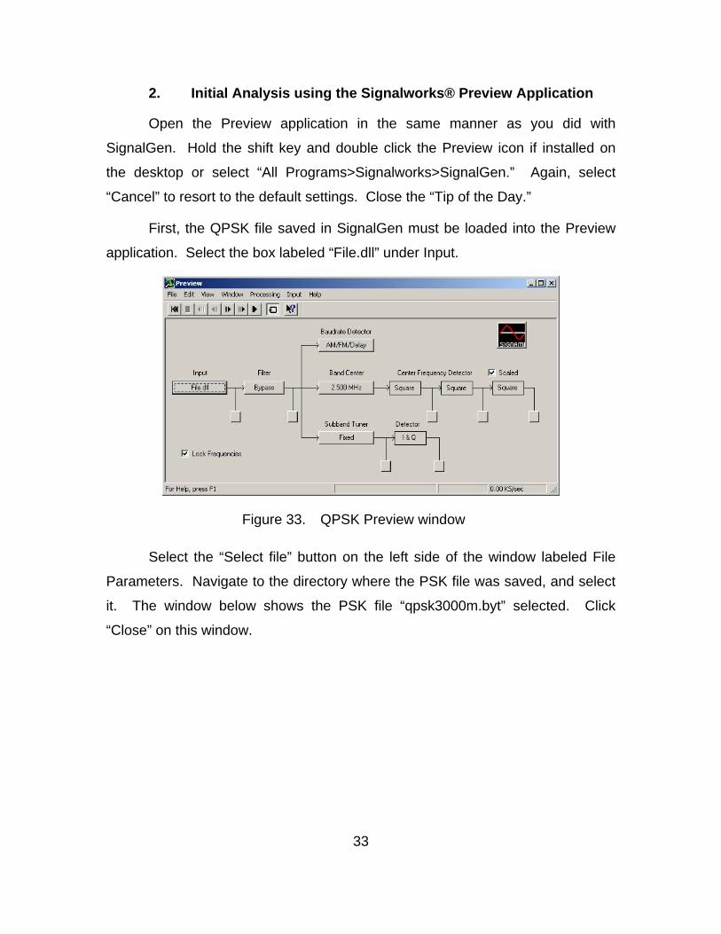
First, the QPSK file saved in SignalGen must be loaded into the Preview
application. Select the box labeled “File.dll” under Input.
Figure 33. QPSK Preview window
Select the “Select file” button on the left side of the window labeled File
Parameters. Navigate to the directory where the PSK file was saved, and select
it. The window below shows the PSK file “qpsk3000m.byt” selected. Click
“Close” on this window.

34
Figure 34. QPSK file input selection
The QPSK signal created earlier is now queued and ready to play and
analyze with the Preview application. Select either the normal play or the
slow motion play button at the top of the Preview window. Select the display
button after the Input to view the QPSK signal.
Figure 35. QPSK Preview test point at file input
The signal should be displayed in the “Input” window and will appear like
the one below.

35
Figure 36. QPSK Preview test point display
The first step in measuring the center frequency of this QPSK is to set the
approximate band center. In the Input display, which shows the QPSK in
frequency (x-axis) and amplitude (y-axis), pull down the Tools menu from the top
and select “Set band center.” Then move the cursor so that it is in the
approximate middle of the QPSK signal. Click on the display to set the band
center. The result is different compared to the PSK signal processed earlier. In
this case, the band center changes to all zeroes.
36
Figure 37. QPSK Preview band center
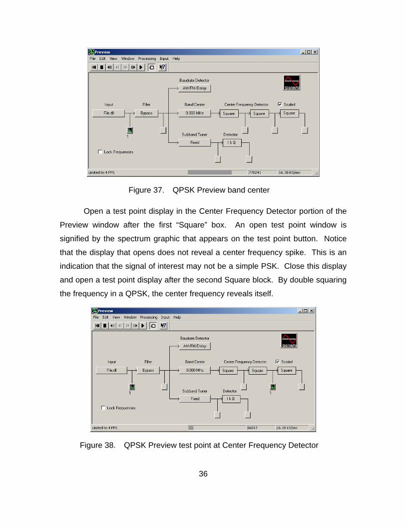
Open a test point display in the Center Frequency Detector portion of the
Preview window after the first “Square” box. An open test point window is
signified by the spectrum graphic that appears on the test point button. Notice
that the display that opens does not reveal a center frequency spike. This is an
indication that the signal of interest may not be a simple PSK. Close this display
and open a test point display after the second Square block. By double squaring
the frequency in a QPSK, the center frequency reveals itself.
Figure 38. QPSK Preview test point at Center Frequency Detector

37
The display that opens is titled “CF^4(2)” which indicates you are looking
at the center frequency double squared. The display will show the QPSK signal
with a prominent spike in the center of the signal. Select the square marker at
the top of the window. The marker should appear at the top of this spike and the
frequency is reflected in the bottom of the window.
Figure 39. QPSK center frequency marker
The center frequency should be 3.0MHz, which corresponds to what was
defined as the carrier frequency in SignalGen when creating this signal. Leave
this window open.
Next, we will derive the symbol (baud) rate. Assure the QPSK signal
sample is playing, in either full motion or slow motion, and then select the
“AM/FM/Delay” button underneath the Baud rate label on the Preview window. A
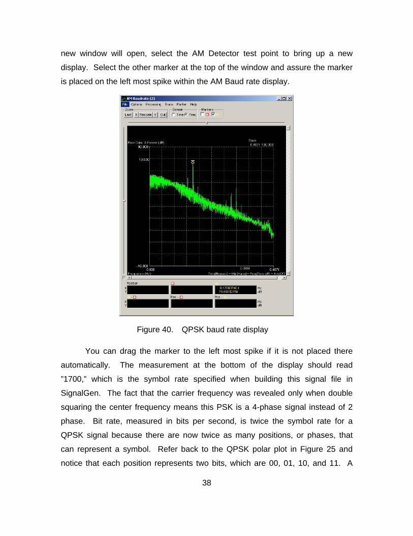
38
new window will open, select the AM Detector test point to bring up a new
display. Select the other marker at the top of the window and assure the marker
is placed on the left most spike within the AM Baud rate display.
Figure 40. QPSK baud rate display
You can drag the marker to the left most spike if it is not placed there
automatically. The measurement at the bottom of the display should read
”1700,” which is the symbol rate specified when building this signal file in
SignalGen. The fact that the carrier frequency was revealed only when double
squaring the center frequency means this PSK is a 4-phase signal instead of 2
phase. Bit rate, measured in bits per second, is twice the symbol rate for a
QPSK signal because there are now twice as many positions, or phases, that
can represent a symbol. Refer back to the QPSK polar plot in Figure 25 and
notice that each position represents two bits, which are 00, 01, 10, and 11. A

39
binary plot allows only a 1 or 0 at each position. Symbol rate is measured in
baud, or symbols per second. The measured symbol rate was 1.7 MBaud and
when doubled results in a bit rate of 3.4 Mbit/s.
Ensure that the carrier frequency and symbol rate displays are active with
their respective markers indicating the measured parameters. Select the “File”
pull-down menu and select “Export / Save for Demod.” The window that appears
shows all active display parameters.
Figure 41. QPSK export/save for Demod
Select “Save Defaults for Demod” at the bottom of the window. This
saves your measured parameters for the Demod.

40
D. ADDITIONAL ANALYSIS WITH DEMOD
1. Procedural Guidance
Demod is Signalworks’® advanced analysis application. It can
demodulate signals and perform bit level analysis. Here, Demod will be used to
define the modulation of the QPSK signal created earlier using SignalGen, which
was initially processed using Preview.
2. Advanced Analysis with Signalworks’® Demod Application
Demod will be used to identify the type of signal that is being analyzed.
Open Demod either by double clicking on the icon or by selecting it from the
Program menu. Do not hold shift. Demod will open with the parameters from
Preview already loaded.
Open the test point after the mixer.
Figure 42. QPSK Demod test point at mixer output
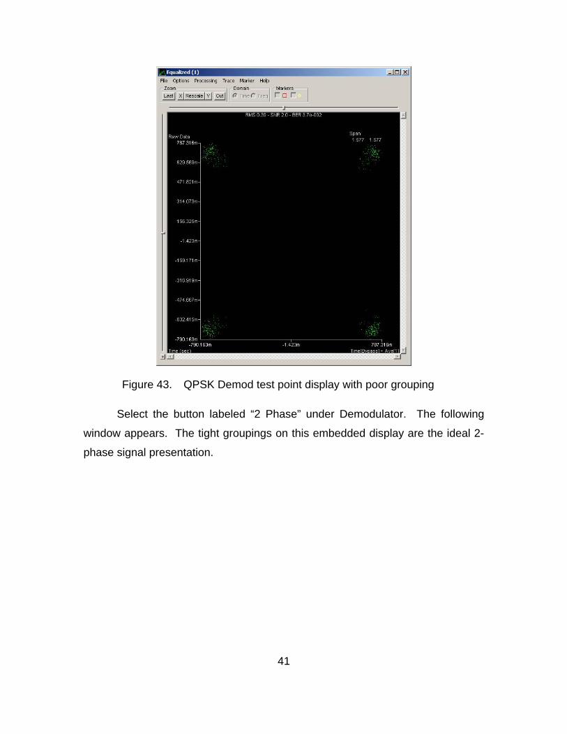
The test point display should like the graphic below titled “Equalized.”
Notice there are four groupings but they are not grouped tightly.
41
Figure 43. QPSK Demod test point display with poor grouping
Select the button labeled “2 Phase” under Demodulator. The following
window appears. The tight groupings on this embedded display are the ideal 2-
phase signal presentation.

42
Figure 44. QPSK PSK demodulator
With the “Demod-PSK Demodulator” window and the “Equalized” windows
both visible, select the “2 Phase” button under Constellation on the “Demod-PSK
Demodulator” window and choose a different constellation until a tight grouping is
presented in the “Equalized” display. Since there are four groupings, try the
various constellations with “4” in the title. The “4 Phase” setting will present a
grouping like the one below, which is the best grouping available.

43
Figure 45. QPSK Demod test point display with optimal grouping
This is the desired presentation, thus confirming this is a Quadrature
Phase-Shift Keyed signal.
E. QPSK ANALYSIS RESULTS
Signalworks® was used to generate and analyze a Quadrature Phase-
shift Keyed signal. Processing the signal with Preview allowed the analyst to
measure the center frequency and baud rate. These measured parameters were
exported to the Demod allowing the user to test different modulation techniques
until a desired grouping was achieved. The first display from the Demod showed
large groupings of dots, which is an indication of the wrong modulation type used
for demodulation or excessive noise in the transmission. By cycling through

44
various modulation types, a tighter grouping of dots was achieved when selecting
4 Phase modulation. Both displays had four points but the phase shift position
on the polar plot was different.
45
IV. QUADRATURE AMPLITUDE MODULATION SIGNAL ANALYSIS
A. OVERVIEW OF QUADRATURE AMPLITUDE MODULATION SIGNALS
1. Signal Characteristics
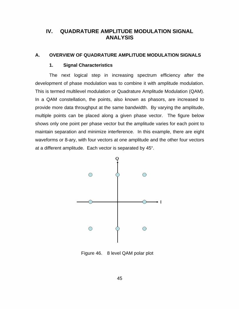
The next logical step in increasing spectrum efficiency after the
development of phase modulation was to combine it with amplitude modulation.
This is termed multilevel modulation or Quadrature Amplitude Modulation (QAM).
In a QAM constellation, the points, also known as phasors, are increased to
provide more data throughput at the same bandwidth. By varying the amplitude,
multiple points can be placed along a given phase vector. The figure below
shows only one point per phase vector but the amplitude varies for each point to
maintain separation and minimize interference. In this example, there are eight
waveforms or 8-ary, with four vectors at one amplitude and the other four vectors
at a different amplitude. Each vector is separated by 45°.
Figure 46. 8 level QAM polar plot
46
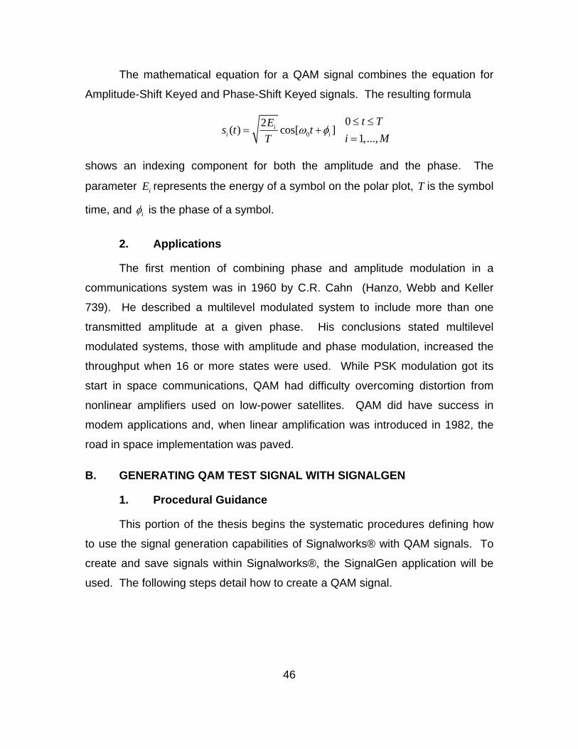
The mathematical equation for a QAM signal combines the equation for
Amplitude-Shift Keyed and Phase-Shift Keyed signals. The resulting formula
0
2( ) cos[ ]i
i i
Es t t
T
0
1,...,
t T
i M
shows an indexing component for both the amplitude and the phase. The
parameter iE represents the energy of a symbol on the polar plot, T is the symbol
time, and i is the phase of a symbol.
2. Applications
The first mention of combining phase and amplitude modulation in a
communications system was in 1960 by C.R. Cahn (Hanzo, Webb and Keller
739). He described a multilevel modulated system to include more than one
transmitted amplitude at a given phase. His conclusions stated multilevel
modulated systems, those with amplitude and phase modulation, increased the
throughput when 16 or more states were used. While PSK modulation got its
start in space communications, QAM had difficulty overcoming distortion from
nonlinear amplifiers used on low-power satellites. QAM did have success in
modem applications and, when linear amplification was introduced in 1982, the
road in space implementation was paved.
B. GENERATING QAM TEST SIGNAL WITH SIGNALGEN
1. Procedural Guidance
This portion of the thesis begins the systematic procedures defining how
to use the signal generation capabilities of Signalworks® with QAM signals. To
create and save signals within Signalworks®, the SignalGen application will be
used. The following steps detail how to create a QAM signal.

47
2. Creating a QAM Signal using the Signalworks® SignalGen Application
To open SignalGen with default parameter settings, hold SHIFT while
double clicking the SignalGen icon if installed on the desktop or select “All
Programs>Signalworks>SignalGen.” The first window that appears allows users
to recall normal parameter settings, user defined settings, or default settings.
Select “Cancel” to use default settings.
Figure 47. Recall default parameters window
Close the “Tip of the Day.” The SignalGen window is now displayed.
Click on the “Bit Operations” button. A new window pops up showing various tool
palette input operations. Drag and drop the “QPSK Perm” and “LRS Encode”
tools into the right-hand side of the window in the “Applied Operations” space.
Click “OK.”
48
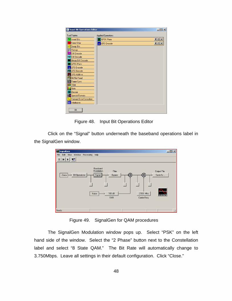
Figure 48. Input Bit Operations Editor
Click on the “Signal” button underneath the baseband operations label in
the SignalGen window.
Figure 49. SignalGen for QAM procedures
The SignalGen Modulation window pops up. Select “PSK” on the left
hand side of the window. Select the “2 Phase” button next to the Constellation
label and select “8 State QAM.” The Bit Rate will automatically change to
3.750Mbps. Leave all settings in their default configuration. Click “Close.”
49
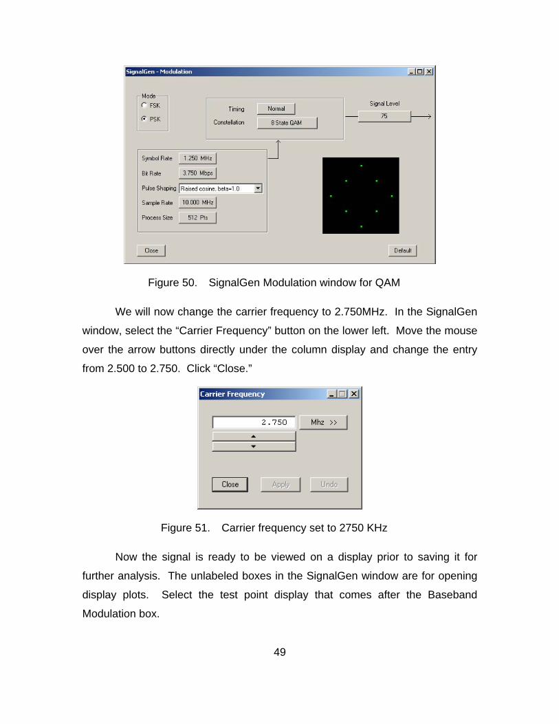
Figure 50. SignalGen Modulation window for QAM
We will now change the carrier frequency to 2.750MHz. In the SignalGen
window, select the “Carrier Frequency” button on the lower left. Move the mouse
over the arrow buttons directly under the column display and change the entry
from 2.500 to 2.750. Click “Close.”
Figure 51. Carrier frequency set to 2750 KHz
Now the signal is ready to be viewed on a display prior to saving it for
further analysis. The unlabeled boxes in the SignalGen window are for opening
display plots. Select the test point display that comes after the Baseband
Modulation box.

50
Figure 52. SignalGen test point of Baseband Modulation output
This will open up a blank Baseband Modulated display similar to an
oscilloscope. With both the SignalGen and the Baseband Modulated windows
within view, select the “play” button at the top left of the SignalGen window.
The display should now show a QAM signal like the one below.

51
Figure 53. QAM Baseband Modulation test point display
Let the signal continue to play and select the “Save as…” button
underneath the Output File label on the SignalGen window. Select the desired
directory where you would like to store this custom file and ensure the extension
is ”byt.” Name the file and select “Save.” When the save is complete, you can
stop playing the QAM signal you just created. The next step is to open Preview
and begin doing the analysis on this signal. Close the SignalGen window.
C. INITIAL QAM ANALYSIS WITH PREVIEW
1. Procedural Guidance
A QAM test signal has just been created using SignalGen. The signal is
ready to be analyzed using the Preview application within Signalworks®. The

52
Preview application allows us to measure some basic parameters and prepare
the signal for further analysis using the Demod application.
2. Initial QAM Analysis using the Signalworks® Preview Application
Open the Preview application in the same manner as you did with
SignalGen. Hold the shift key and double click the Preview icon if installed on
the desktop or select “All Programs>Signalworks>SignalGen.” Again, select
“Cancel” to resort to the default settings. Close the “Tip of the Day.”
First, the QAM file saved in SignalGen must be loaded into the Preview
application. Select the box labeled “File.dll” under Input.
Figure 54. QAM Preview window
Select the “Select file” button on the left side of the window labeled File
Parameters. Navigate to the directory where the QAM file was saved and select
it. The window below shows the QAM file “8qam.byt” selected. Click “Close” on
this window.

53
Figure 55. QAM file input selection
The QAM signal created earlier is now queued and ready to play and
analyze with the Preview application. Select either the normal play or the
slow motion play button at the top of the Preview window. Select the display
button after the Input to view the QAM signal.
Figure 56. QAM Preview test point at file input
The signal should be displayed in the “Input” window and will look like the
one below.
54
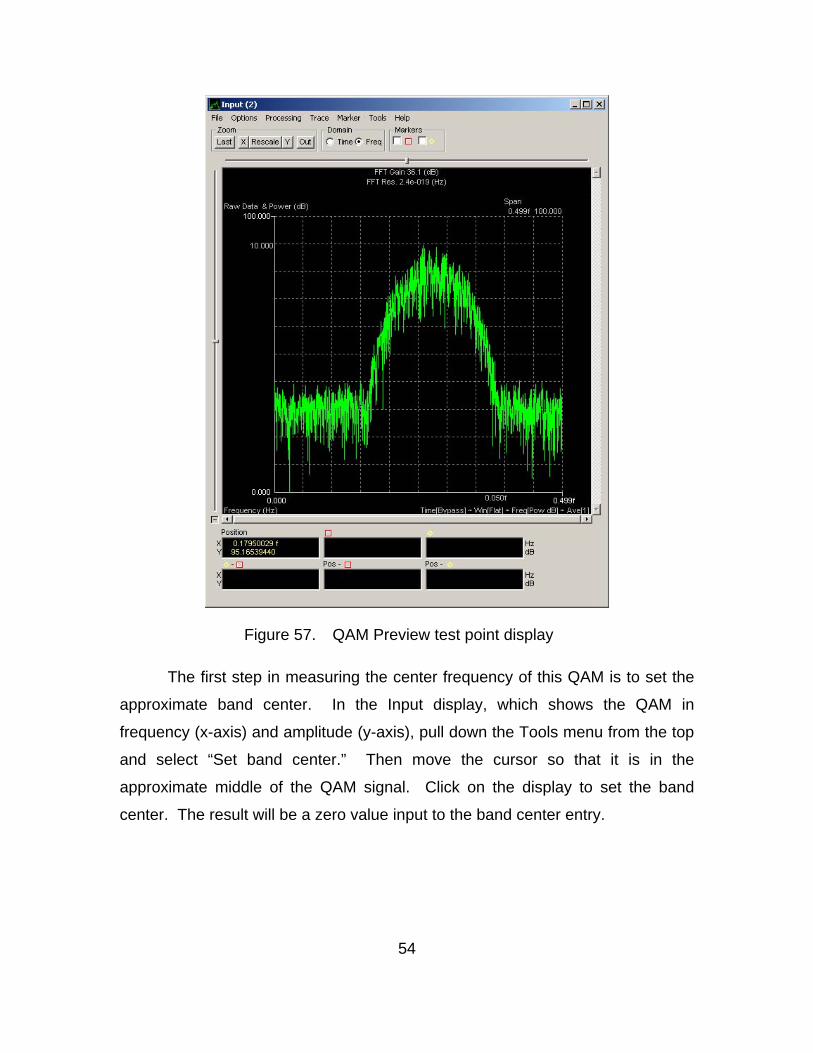
Figure 57. QAM Preview test point display
The first step in measuring the center frequency of this QAM is to set the
approximate band center. In the Input display, which shows the QAM in
frequency (x-axis) and amplitude (y-axis), pull down the Tools menu from the top
and select “Set band center.” Then move the cursor so that it is in the
approximate middle of the QAM signal. Click on the display to set the band
center. The result will be a zero value input to the band center entry.

55
Figure 58. QAM Preview band center specification
Open a test point display in the Center Frequency Detector portion of the
Preview window after the first “Square” box. Notice that the display that opens
does not reveal a center frequency spike. This is an indication that the signal of
interest may not be a simple PSK. Close this display and open a test point
display after the second Square block. By double squaring the frequency in a
QAM, the center frequency will be revealed.
Figure 59. QAM Preview test point at Center Frequency Detector

56
The display that opens is titled “CF^4(2)” which indicates you are looking
at the center frequency double squared. The display will show the QAM signal
with a prominent spike in the center of the signal. Select the square marker at
the top of the window. The marker should appear at the top of this spike and the
frequency is reflected in the bottom of the window.
Figure 60. QAM center frequency marker
The center frequency should be 2.750 MHz, which corresponds to what
was defined as the carrier frequency in SignalGen when creating this signal.
Leave this window open.
Next, we will derive the symbol (baud) rate. Assure the QAM signal
sample is playing, in either full motion or slow motion, and then select the
“AM/FM/Delay” button underneath the Baudrate label on the Preview window. A

57
new window will open, select the AM Detector test point to bring up a new
display. Select the other marker at the top of the window and assure the marker
is placed on the left most spike within the AM Baudrate display.
Figure 61. QAM baud rate display
You can drag the marker to the left most spike if it is not placed there
automatically. The measurement at the bottom of the display should read
”1250,” which is the symbol rate specified when building this signal file in
SignalGen. The fact that the carrier frequency was revealed only when double
squaring the center frequency means this is a quadrature signal instead of a
single carrier signal. Bit rate, measured in bits per second, is twice the symbol
rate for a QAM signal because there are now twice as many positions, or phase-

58
amplitude combinations, that can represent a symbol. Like the QPSK polar plot
depicted in Figure 25, each position represents two bits; 00, 01, 10, and 11. A
binary plot allows only a 1 or 0 at each position. Symbol rate is measured in
baud, or symbols per second. The measured symbol rate was 1.25 MBaud and
when doubled results in a bit rate of 2.5 Mbit/s.
Ensure that the carrier frequency and symbol rate displays are active, with
their respective markers indicating the measured parameters. Select the “File”
pull-down menu and select “Export / Save for Demod.” The window that appears
shows all active display parameters.
Figure 62. QAM export/save for Demod
Select “Save Defaults for Demod” at the bottom of the window. This
saves your measured parameters for the Demod.
59
D. ADDITIONAL QAM ANALYSIS WITH DEMOD
1. Procedural Guidance
Demod is Signalworks’® advanced analysis application. It can
demodulate signals and perform bit level analysis. Here, Demod will be used to
define the modulation of the QAM signal created earlier using SignalGen, which
was initially processed using Preview.
2. Advanced QAM Analysis with the Signalworks® Demod Application
Demod will be used to identify the type of signal that is being analyzed.
Open Demod by double either clicking on the icon or selecting it from the
Program menu. Do not hold shift. Demod will open with the parameters from
Preview already loaded.
Open the test point after the mixer.
Figure 63. QAM Demod test point at mixer output
The test point display should like the graphic below titled “Equalized.”
Notice there are eight groupings, but they are not grouped tightly.

60
Figure 64. QAM Demod test point display with poor groupings
Select the button labeled “2 Phase” under Demodulator. The following
window appears. The tight groupings on this embedded display are the ideal 2-
phase signal presentation.

61
Figure 65. QAM Demod PSK Demodulator window
With the “Demod-PSK Demodulator” window and the “Equalized” windows
both visible, select the “2 Phase” button under Constellation on the “Demod-PSK
Demodulator” window and choose a different constellation until a tight grouping is
presented in the “Equalized” display. Since there are eight groupings, try the
various constellations with “8” in the title. The “8 State QAM” setting will present
a grouping like the one shown below in Figure 66, which has been annotated to
explain the varying amplitudes and phases of a QAM signal.

62
Figure 66. QAM Demod test point display with acceptable groupings
Similar to a QPSK signal, various phases are used in a QAM signal to
represent symbols. Now the added parameter of amplitude is incorporated to
increase the number of possible symbols. This variation in amplitude is shown
with the white arrows. The grouping with a 0° shift is higher in amplitude than the
grouping at the 45° shift. The variation in amplitude and phase allows for more
symbol positions while maintaining separation from other positions to minimize
interference. The display in Figure 66 is the desired presentation, thus this signal
is in fact an eight State-Quadrature Amplitude Modulated signal. In a normal
QAM signal, symbol rate is based on four data signals 90° out of phase. Since
this is an 8 State signal, multiply the symbol rate by 3 (8=2^3) to determine the
bit rate. In this case, 1.250 MHz x 3 = 3.750 Mbps bit rate.
63
E. WORKING WITH ADVANCED QAM SIGNALS
1. Beyond 8-State QAM
Up to this point, the analysis has been focused on an 8-State QAM signal.
This section supplements the procedures already discussed to allow the user to
generate and analyze a 16- and 64-State QAM. In order to achieve more points
in the constellation, the system would have to implement more amplitude and
phase shifts. This increases the data throughput at the cost of more induced
error since the spacing between constellation points has decreased.
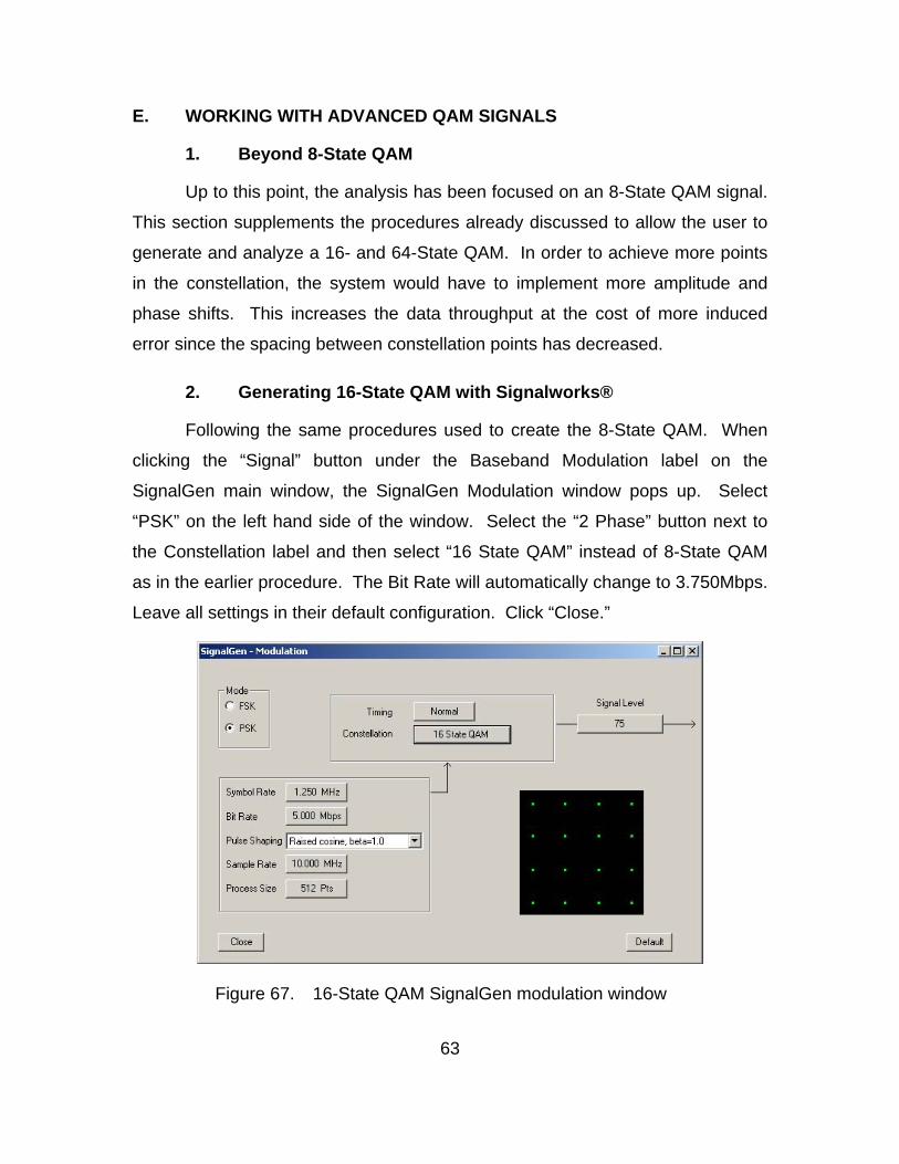
2. Generating 16-State QAM with Signalworks®
Following the same procedures used to create the 8-State QAM. When
clicking the “Signal” button under the Baseband Modulation label on the
SignalGen main window, the SignalGen Modulation window pops up. Select
“PSK” on the left hand side of the window. Select the “2 Phase” button next to
the Constellation label and then select “16 State QAM” instead of 8-State QAM
as in the earlier procedure. The Bit Rate will automatically change to 3.750Mbps.
Leave all settings in their default configuration. Click “Close.”
Figure 67. 16-State QAM SignalGen modulation window
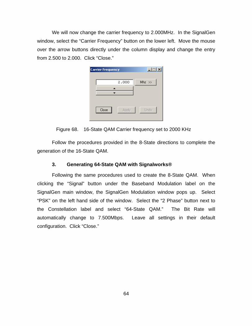
64
We will now change the carrier frequency to 2.000MHz. In the SignalGen
window, select the “Carrier Frequency” button on the lower left. Move the mouse
over the arrow buttons directly under the column display and change the entry
from 2.500 to 2.000. Click “Close.”
Figure 68. 16-State QAM Carrier frequency set to 2000 KHz
Follow the procedures provided in the 8-State directions to complete the
generation of the 16-State QAM.
3. Generating 64-State QAM with Signalworks®
Following the same procedures used to create the 8-State QAM. When
clicking the “Signal” button under the Baseband Modulation label on the
SignalGen main window, the SignalGen Modulation window pops up. Select
“PSK” on the left hand side of the window. Select the “2 Phase” button next to
the Constellation label and select “64-State QAM.” The Bit Rate will
automatically change to 7.500Mbps. Leave all settings in their default
configuration. Click “Close.”

65
Figure 69. 64-State QAM SignalGen modulation window
We will now change the carrier frequency to 2.600MHz. In the SignalGen
window, select the “Carrier Frequency” button on the lower left. Move the mouse
over the arrow buttons directly under the column display and change the entry
from 2.500 to 2.600. Click “Close.”
Figure 70. 64-State QAM Carrier frequency set to 2,600 KHz
Follow the procedures provided in the 8-State directions to complete the
generation of the 64-State QAM.
4. Initial analysis of 16-State QAM with Preview
The procedure within Preview when analyzing 16-State QAM is the same
as 8-State QAM up to the point where center frequency is measured. Open a
test point display in the Center Frequency Detector portion of the Preview

66
window after the first “Square” box. Notice that the display the opens does not
reveal a center frequency spike. This is an indication that the signal of interest
may not be a more simple two phase PSK. Close this display and open a test
point display after the second Square block. By double squaring the frequency in
a QAM, the center frequency will be revealed.
Figure 71. 16-State QAM Preview test point for double squared center frequency
The display that opens is titled “CF^4(2)” which indicates you are looking
at the center frequency double squared. The display will show the QAM signal
with a prominent spike in the center of the signal. Select the square marker at
the top of the window. The marker should appear at the top of this spike and the
frequency is reflected in the bottom of the window.

67
Figure 72. 16-State QAM test point display for double carrier frequency
The center frequency should be 2.000 MHz, which corresponds to what
was defined as the carrier frequency in SignalGen when creating this signal.
Leave this window open.
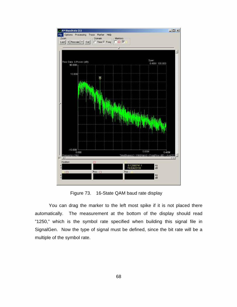
Next, we will derive the symbol (baud) rate. Assure the QAM signal
sample is playing in full or slow motion, and then select the “AM/FM/Delay”
button underneath the Baudrate label on the Preview window. A new window will
open, select the AM Detector test point to bring up a new display. Select the
other marker at the top of the window and assure the marker is placed on the
left-most spike within the AM Baudrate display.
68
Figure 73. 16-State QAM baud rate display
You can drag the marker to the left most spike if it is not placed there
automatically. The measurement at the bottom of the display should read
”1250,” which is the symbol rate specified when building this signal file in
SignalGen. Now the type of signal must be defined, since the bit rate will be a
multiple of the symbol rate.

69
Ensure that the carrier frequency and symbol rate displays are active with
their respective markers indicating the measured parameters. Select the “File”
pull-down menu and select “Export / Save for Demod.” The window that appears
shows all active display parameters.
Figure 74. 16-State QAM export/save for Demod window
Select “Save Defaults for Demod” at the bottom of the window. This
saves your measured parameters for the Demod. This completes the
procedures for generating a 16-State QAM. The next step is to start analysis in
Preview.
5. Initial Analysis of 64-State QAM with Preview
The procedure within Preview when analyzing 64-State QAM is the same
as 8-State QAM up to the point where center frequency is measured. Open a
test point display in the Center Frequency Detector portion of the Preview
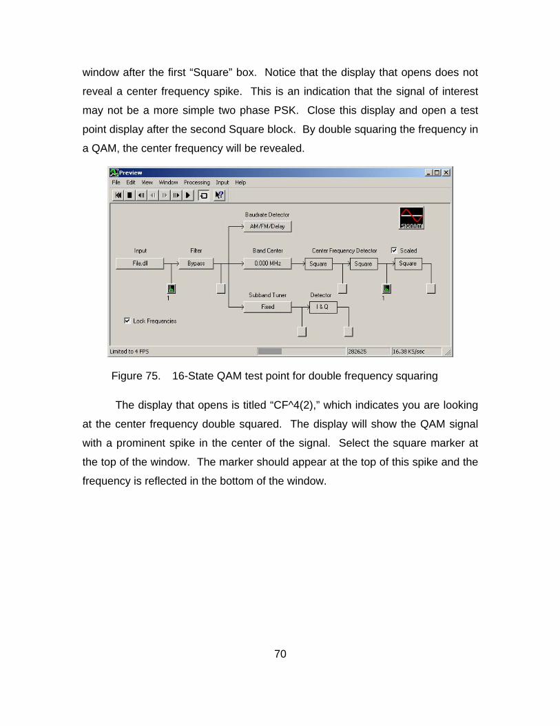
70
window after the first “Square” box. Notice that the display that opens does not
reveal a center frequency spike. This is an indication that the signal of interest
may not be a more simple two phase PSK. Close this display and open a test
point display after the second Square block. By double squaring the frequency in
a QAM, the center frequency will be revealed.
Figure 75. 16-State QAM test point for double frequency squaring
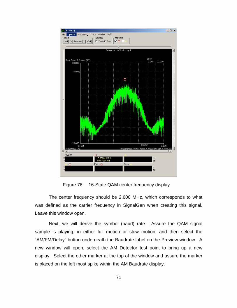
The display that opens is titled “CF^4(2),” which indicates you are looking
at the center frequency double squared. The display will show the QAM signal
with a prominent spike in the center of the signal. Select the square marker at
the top of the window. The marker should appear at the top of this spike and the
frequency is reflected in the bottom of the window.
71
Figure 76. 16-State QAM center frequency display
The center frequency should be 2.600 MHz, which corresponds to what
was defined as the carrier frequency in SignalGen when creating this signal.
Leave this window open.
Next, we will derive the symbol (baud) rate. Assure the QAM signal
sample is playing, in either full motion or slow motion, and then select the
“AM/FM/Delay” button underneath the Baudrate label on the Preview window. A
new window will open, select the AM Detector test point to bring up a new
display. Select the other marker at the top of the window and assure the marker
is placed on the left most spike within the AM Baudrate display.

72
Figure 77. 16-State QAM baud rate display
You can drag the marker to the left most spike if it is not placed there
automatically. The measurement at the bottom of the display should read
”1250,” which is the symbol rate specified when building this signal file in
SignalGen. Now the type of signal must be defined since the bit rate will be a
multiple of the symbol rate.
Ensure that the carrier frequency and symbol rate displays are active with
their respective markers indicating the measured parameters. Select the “File”
pull-down menu and select “Export / Save for Demod.” The window that appears
shows all active display parameters.
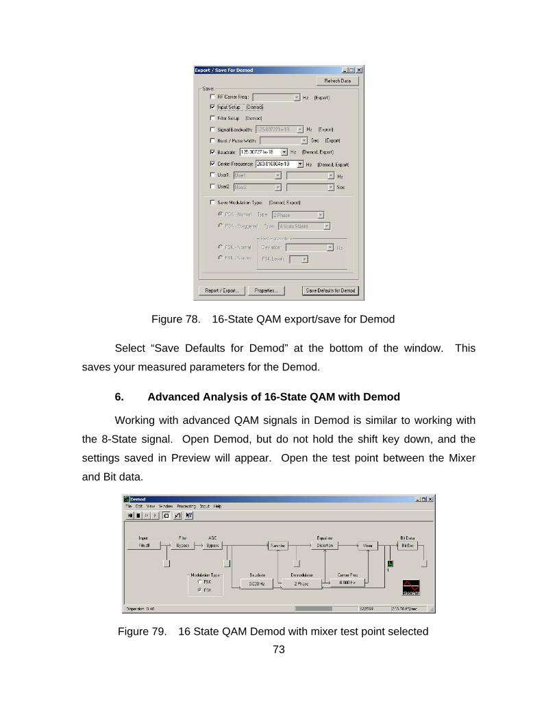
73
Figure 78. 16-State QAM export/save for Demod
Select “Save Defaults for Demod” at the bottom of the window. This
saves your measured parameters for the Demod.
6. Advanced Analysis of 16-State QAM with Demod
Working with advanced QAM signals in Demod is similar to working with
the 8-State signal. Open Demod, but do not hold the shift key down, and the
settings saved in Preview will appear. Open the test point between the Mixer
and Bit data.
Figure 79. 16 State QAM Demod with mixer test point selected
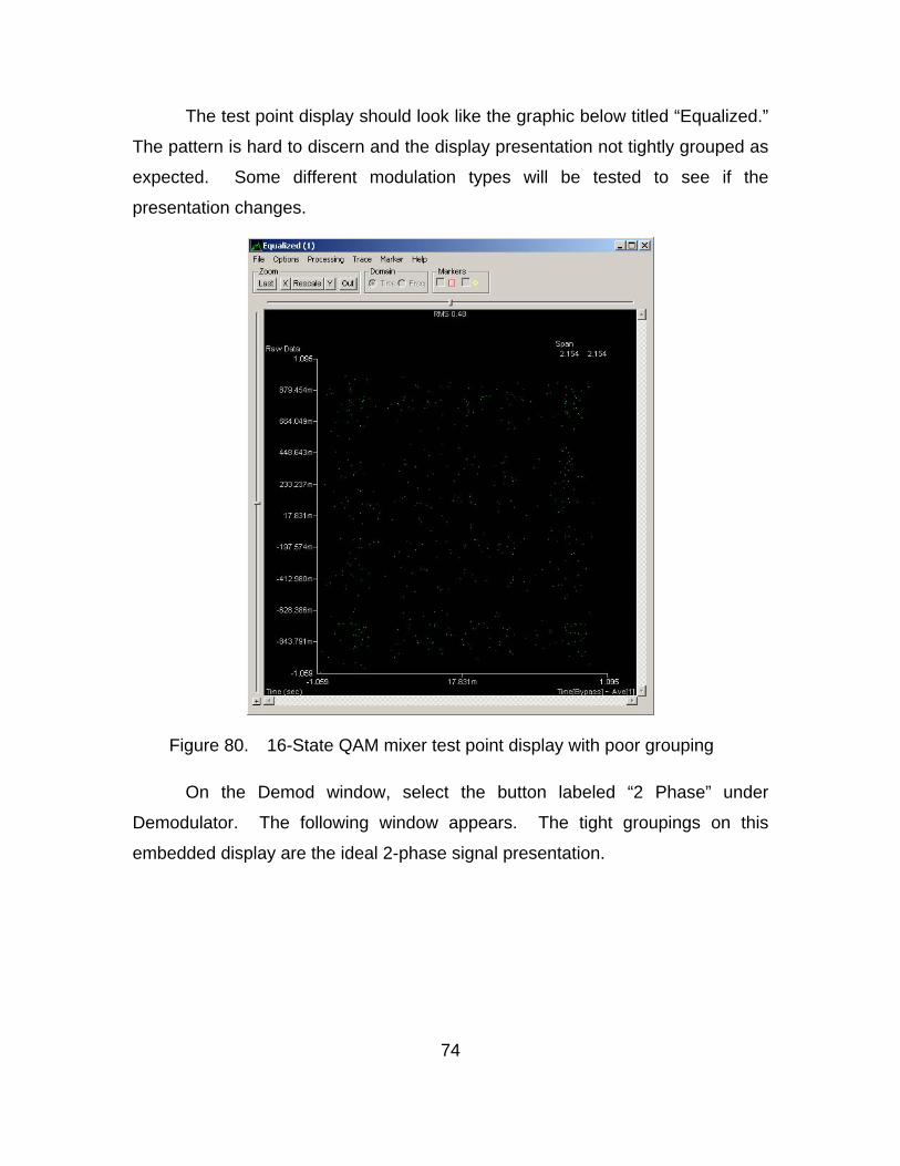
74
The test point display should look like the graphic below titled “Equalized.”
The pattern is hard to discern and the display presentation not tightly grouped as
expected. Some different modulation types will be tested to see if the
presentation changes.
Figure 80. 16-State QAM mixer test point display with poor grouping
On the Demod window, select the button labeled “2 Phase” under
Demodulator. The following window appears. The tight groupings on this
embedded display are the ideal 2-phase signal presentation.
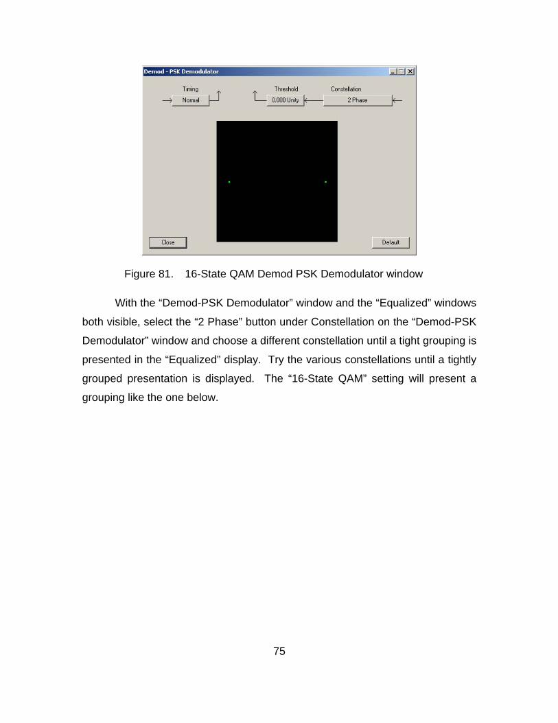
75
Figure 81. 16-State QAM Demod PSK Demodulator window
With the “Demod-PSK Demodulator” window and the “Equalized” windows
both visible, select the “2 Phase” button under Constellation on the “Demod-PSK
Demodulator” window and choose a different constellation until a tight grouping is
presented in the “Equalized” display. Try the various constellations until a tightly
grouped presentation is displayed. The “16-State QAM” setting will present a
grouping like the one below.
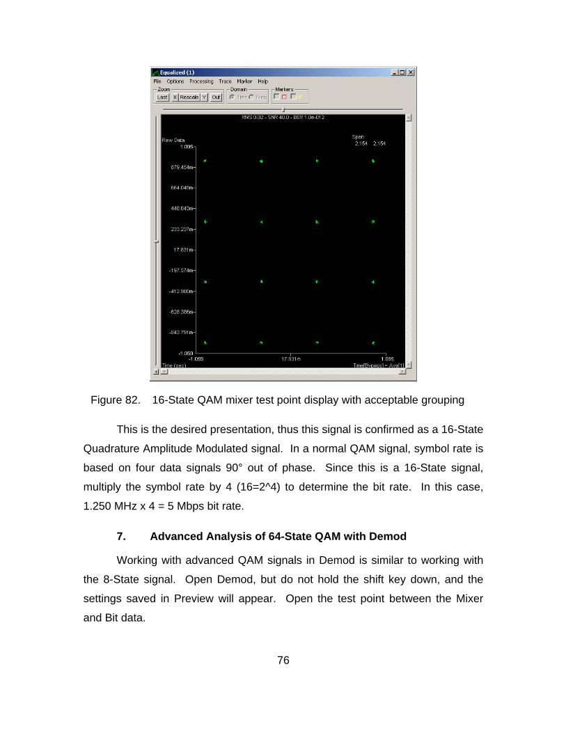
76
Figure 82. 16-State QAM mixer test point display with acceptable grouping
This is the desired presentation, thus this signal is confirmed as a 16-State
Quadrature Amplitude Modulated signal. In a normal QAM signal, symbol rate is
based on four data signals 90° out of phase. Since this is a 16-State signal,
multiply the symbol rate by 4 (16=2^4) to determine the bit rate. In this case,
1.250 MHz x 4 = 5 Mbps bit rate.
7. Advanced Analysis of 64-State QAM with Demod
Working with advanced QAM signals in Demod is similar to working with
the 8-State signal. Open Demod, but do not hold the shift key down, and the
settings saved in Preview will appear. Open the test point between the Mixer
and Bit data.
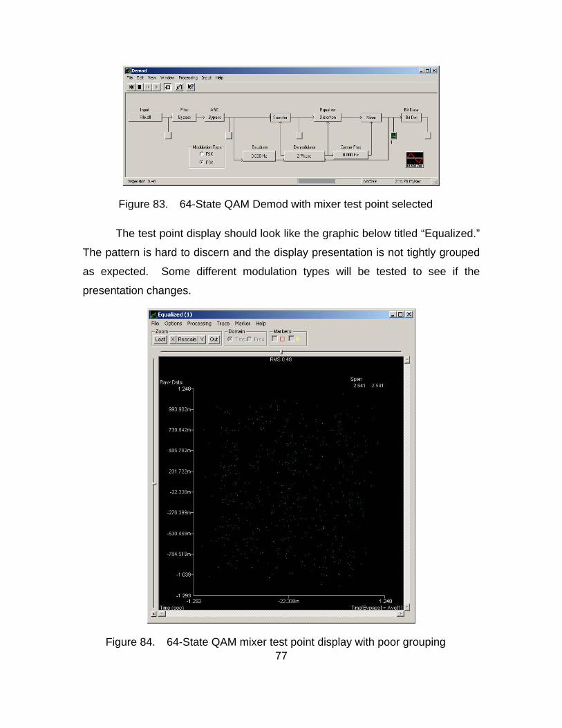
77
Figure 83. 64-State QAM Demod with mixer test point selected
The test point display should look like the graphic below titled “Equalized.”
The pattern is hard to discern and the display presentation is not tightly grouped
as expected. Some different modulation types will be tested to see if the
presentation changes.
Figure 84. 64-State QAM mixer test point display with poor grouping

78
Select the button labeled “2 Phase” under Demodulator. The following
window appears. The tight groupings on this embedded display are the ideal 2-
phase signal presentation.
Figure 85. 64-State QAM Demod PSK Demodulator window
With the “Demod-PSK Demodulator” window and the “Equalized” windows
both visible, select the “2 Phase” button under Constellation on the “Demod-PSK
Demodulator” window and choose a different constellation until a tight grouping is
presented in the “Equalized” display. Try the various constellations until a tightly
grouped presentation is displayed. The “64-State QAM” setting will present a
grouping like the one below.

79
Figure 86. 64-State QAM mixer test point display with acceptable grouping
This is the desired presentation, thus this signal is confirmed as a 64-State
Quadrature Amplitude Modulated signal. In a normal QAM signal, symbol rate is
based on four data signals 90° out of phase. Since this is a 64-State signal,
multiply the symbol rate by 6 (64=2^6) to determine the bit rate. In this case,
1.250 MHz x 6 = 7.5 Mbps bit rate.
F. QAM ANALYSIS RESULTS
Signalworks® was used to generate and analyze a Quadrature Amplitude
Modulated signal. Processing the signal with Preview allowed the analyst to
measure the center frequency and baud rate. These measured parameters were
exported to the Demod, allowing the user to test different modulation techniques
until a desired grouping was achieved. Initial views of the modulation display
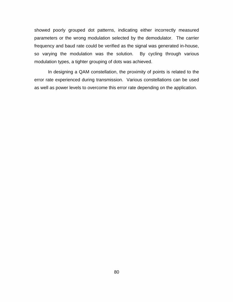
80
showed poorly grouped dot patterns, indicating either incorrectly measured
parameters or the wrong modulation selected by the demodulator. The carrier
frequency and baud rate could be verified as the signal was generated in-house,
so varying the modulation was the solution. By cycling through various
modulation types, a tighter grouping of dots was achieved.
In designing a QAM constellation, the proximity of points is related to the
error rate experienced during transmission. Various constellations can be used
as well as power levels to overcome this error rate depending on the application.

81
V. WI-FI SIGNAL ANALYSIS
A. OVERVIEW OF WIFI SIGNALS
1. Signal Characteristics
This section discusses analysis of a signal sample file included with the
Signalworks® installation. There are two Wi-Fi signals included in the sample
file. For this analysis, the file title “wifi1.wrd” will be used. This file replicates an
802.11b standard Wi-Fi signal. The 802.11b standard is an extension of the
802.11 standard that increases the data throughput up to 11 Mbps using a
frequency of 2.4 GHz range (Comer 719). The 802.11b standard was ratified in
1999, and products using the new extended standard reached the market in
2000. This new standard implemented Direct Sequence Spread Spectrum to
increase data rate and maintain acceptable bit error rates (Heegard et al. 64).
2. Application
Initially, 802.11b networks were an improvement over original wireless
technology established by the 802.11 standard. Now, due to interference with
other devices operating at 2.4 GHz such as Bluetooth appliances, cordless
phones, and microwaves, the 802.11b standard is less prevalent. Most modern
802.11g routers and access points are, however, backwards compatible with
802.11b.
B. INITIAL ANALYSIS WITH PREVIEW
1. Procedural Guidance
Signalworks® is limited in its ability to generate an 802.11b standard
signal within SignalGen. Signals must be generated via an alternative source
such as Matlab®. For this procedure, the Wi-Fi signal used for analysis will
come from the sample signal file that is part of the standard Signalworks®
installation. The signal will be initially processed in Preview and then exported to
Demod for bit analysis.

82
2. Initial Analysis using the Signalworks® Preview Application
Open Preview by double clicking the Preview icon or selecting it from the
Program menu under the Signalworks® folder. Remember to hold the shift key
down prior to clicking on Preview in order to bring up the default parameters
selection window. Select Cancel on the Recall window.
Figure 87. Recall window
Select Close on the “Tip of the Day” window. Click on the File.dll button to
open the File Input window and click on the Select File button. Select the file
named “wifi1.wrd.” Do not close the File Input window. At this point, it is
necessary to capture only a portion of this signal since the sample file has
moments when the signal is active and moments when the signal is idle. For the
purpose of analysis, only the active portion of the sample file is needed. Place
the File Input window on one side of the screen and then open the test point just
after the Input portion of the Preview window. In this next step, the Start and
Stop features of Preview will be used. The buttons to control the Start and Stop
function are located on the File Input window, which should still be open on your
screen.
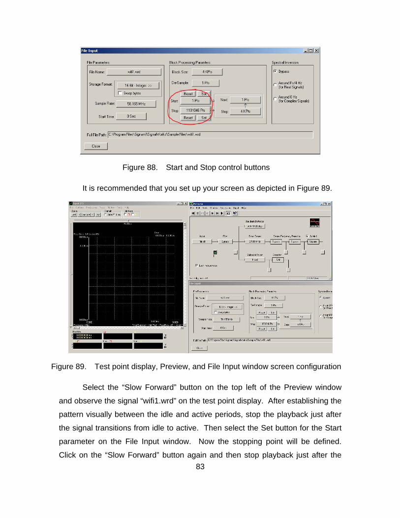
83
Figure 88. Start and Stop control buttons
It is recommended that you set up your screen as depicted in Figure 89.
Figure 89. Test point display, Preview, and File Input window screen configuration
Select the “Slow Forward” button on the top left of the Preview window
and observe the signal “wifi1.wrd” on the test point display. After establishing the
pattern visually between the idle and active periods, stop the playback just after
the signal transitions from idle to active. Then select the Set button for the Start
parameter on the File Input window. Now the stopping point will be defined.
Click on the “Slow Forward” button again and then stop playback just after the

84
signal transitions to idle. Use the “Step Back” button to go backward frame by
frame until the first frame with the active signal is observed. Select the Set
button for the Stop parameter on the File Input window. One active cycle of the
signal has now been captured and will be used by Preview. If this procedure has
been performed correctly, a constant active signal will be observed in the test
point display when selecting the Play button. Once this is verified, close the File
Input window.
The next step is to set up a filter to discard all but the peak power of the
signal. With the Input test point display window active, select the Tools pull down
menu and click on Filter Setup. Drag the cursor left to right across the peak of
the signal. The resulting display will appear similar to Figure 90.

85
Figure 90. Filter Setup for wifi1.wrd
Close the Input test point display and select the first test point display in
the Center Frequency Detector. Click on the red box marker at the top of the
screen to measure the center frequency of this signal. Leave this display open.
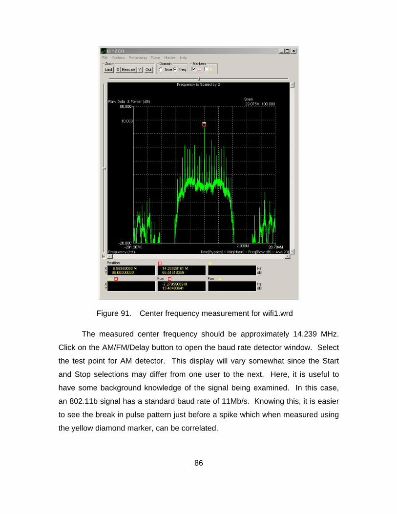
86
Figure 91. Center frequency measurement for wifi1.wrd
The measured center frequency should be approximately 14.239 MHz.
Click on the AM/FM/Delay button to open the baud rate detector window. Select
the test point for AM detector. This display will vary somewhat since the Start
and Stop selections may differ from one user to the next. Here, it is useful to
have some background knowledge of the signal being examined. In this case,
an 802.11b signal has a standard baud rate of 11Mb/s. Knowing this, it is easier
to see the break in pulse pattern just before a spike which when measured using
the yellow diamond marker, can be correlated.

87
Figure 92. Baudrate detector display with 11Mb/s wifi1.wrd signal
Leave this display open. Next open the test point display after the I & Q
Detector. The display will appear as below due to the center frequency not being
specific.

88
Figure 93. Inaccurate center frequency depicted in I&Q test point display
Leave this display open and select the Fixed button under Sub band tuner
on the Preview window. Click on the Frequency button on the Fixed Sub band
Tuner window. Using the frequency adjustment window, vary the frequency
slightly to create a change in the appearance of the IQ display. The intent is to
stop the spinning appearance on the display. Change the measurement units on
the Frequency window to Hz. Start from the fourth column from the left and
begin making changes to the frequency. Keep moving right and adjust the
frequency to slow down and eventually stop the signal in the IQ display. The
resulting display will be similar to Figure 94.

89
Figure 94. IQ display with adjusted frequency
This signal is ready to export to the Demod application. From the Preview
window, select “File,” then “Export/Save for Demod.” Make sure that the center
frequency the appears in the Export/Save for Demod window is the same as
what was just adjusted in the Sub band Tuner. If it is not, use the pull down
menu next to the Center Frequency line to select the correct center frequency. In
the bottom half of the Export/Save for Demod window, checkmark Save
Modulation Type and select PSK Normal with type “2 Phase.”

90
Figure 95. Export/Save for Demod window
Once this has been completed, select Save Defaults for Demod. Close
the Preview window and all subordinate windows.
C. ADDITIONAL WIFI ANALYSIS WITH DEMOD
1. Procedural Guidance
Using the Demod application within Signalworks®, this wireless signal can
be demodulated down to the bit level allowing the analyst to break out the Media
Access Control (MAC) address.
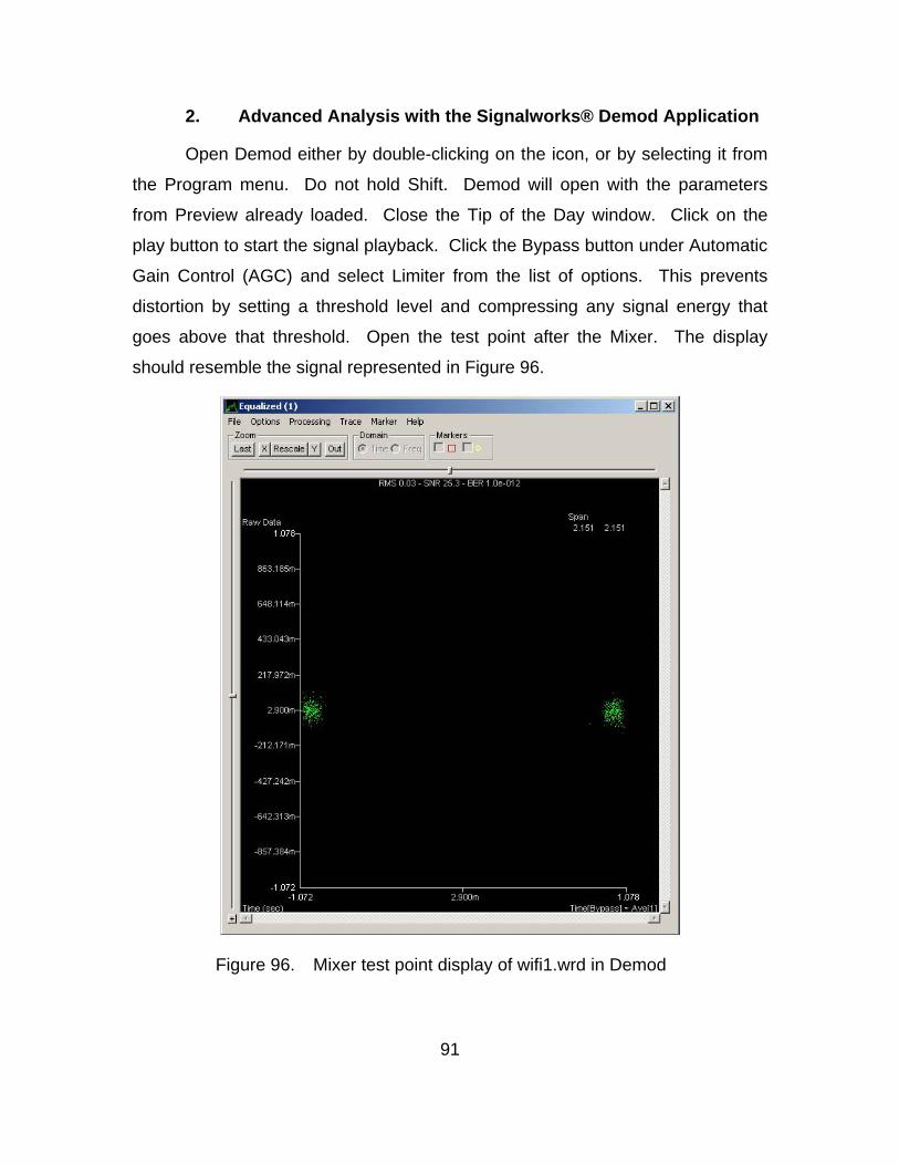
91
2. Advanced Analysis with the Signalworks® Demod Application
Open Demod either by double-clicking on the icon, or by selecting it from
the Program menu. Do not hold Shift. Demod will open with the parameters
from Preview already loaded. Close the Tip of the Day window. Click on the
play button to start the signal playback. Click the Bypass button under Automatic
Gain Control (AGC) and select Limiter from the list of options. This prevents
distortion by setting a threshold level and compressing any signal energy that
goes above that threshold. Open the test point after the Mixer. The display
should resemble the signal represented in Figure 96.
Figure 96. Mixer test point display of wifi1.wrd in Demod

92
At this point, the signal is prepared to be analyzed at the bit level. Open
the test point after Bit Data in the Demod window. The display will resemble
Figure 97.
Figure 97. Bit Operations display for wifi1.wrd
Click on the Bit Ops button in the Processing section of the Bit Operations
display. The window that opens is the Bit Operations Editor. Click and drag the
Keep/Skip tool from the left menu on the left into the Applied Operations window
on the right side. Click once on the Keep/Skip tool that was just placed in the
Applied Operations to pull down the expanded functions. In order to remove the
Walsh coding from this signal, the Keep/Skip must be set to keep one and skip
twenty-one. Put the cursor in the window and change the Keep/Skip setting to
“(1, 21).”

93
Figure 98. Bit Operations Editor with Keep/Skip tool with expanded functions
Click on the apply button to save the Keep/Skip settings. This window will
be used later and can be minimized for now.
On the Bit Operations display, select Processing from the top menu and
then select Search and Scan. Click on the Linear Recursive Sequence tab and
click the LRS Quick Scan button.
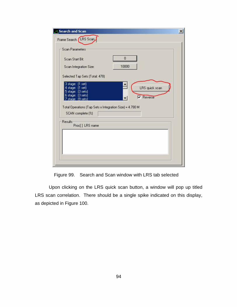
94
Figure 99. Search and Scan window with LRS tab selected
Upon clicking on the LRS quick scan button, a window will pop up titled
LRS scan correlation. There should be a single spike indicated on this display,
as depicted in Figure 100.

95
Figure 100. LRS Scan Correlation with single spike
Once the single spike has been verified, close this window and return to
the Search and Scan window. At the bottom of the window, there should now be
a list of results. Double click the result “R7+R4+1.”
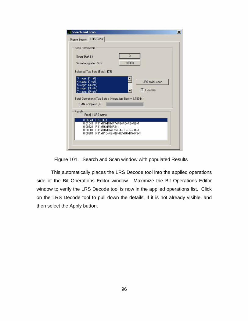
96
Figure 101. Search and Scan window with populated Results
This automatically places the LRS Decode tool into the applied operations
side of the Bit Operations Editor window. Maximize the Bit Operations Editor
window to verify the LRS Decode tool is now in the applied operations list. Click
on the LRS Decode tool to pull down the details, if it is not already visible, and
then select the Apply button.
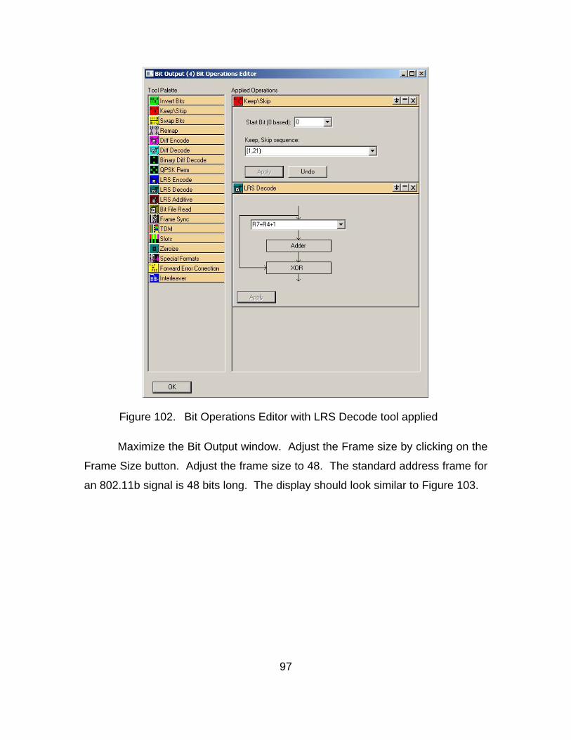
97
Figure 102. Bit Operations Editor with LRS Decode tool applied
Maximize the Bit Output window. Adjust the Frame size by clicking on the
Frame Size button. Adjust the frame size to 48. The standard address frame for
an 802.11b signal is 48 bits long. The display should look similar to Figure 103.

98
Figure 103. Bit Output display with 48 bit frame size
Select Display at the top of the Bit Output window and select “4 Bit 0-F
Hex.” The display of bits will change to hex characters and should resemble
Figure 104.

99
Figure 104. Bit Output with 0-F Hex display
At this point, the MAC address of the computer sending traffic can be
determined by locating the first twelve characters after the string of “F”
characters. Figure 105 highlights a few MAC addresses following strings of F
characters.

100
Figure 105. HEX display with highlighted MAC addresses
D. WIFI ANALYSIS RESULTS
This process dealt with a sample file of an 802.11b standard WIFI signal
that is resident along with other sample files in the normal Signalworks®
installation. Since the signal had periods of transmit and periods of idle, the time
frame of the signal file to import into Preview was specified using Start and Stop
settings so that only periods of transmit were analyzed. There were a few
differences in the procedure for this signal that were done to highlight different
features of Signalworks®. Instead of estimating a band center, a filter was used
to exclude all but the peak energy of the signal. The analyst also looked at the
I&Q display in Preview to make a frequency adjustment of the center frequency.
Within Demod, the analyst worked down to the bit level and derived the MAC
address of computers sending traffic.

101
VI. SUMMARY AND RECOMMENDATIONS FOR FUTURE WORK
A. SUMMARY
1. Installation and Operation
For the duration of this project, Signalworks® 4.0 was installed on a
Compaq V2000 laptop computer with 32-bit Windows Vista operating system.
The laptop processor is an AMD Turion 64-bit chip operating at a speed of
1.8GHz with two gigabytes of RAM. This exceeded the minimum requirements
specified for Signalworks®. Specifications state that as little as 128Mb of RAM
are acceptable. Specifications also state that Signalworks® can be installed on
other Windows platforms including Windows XP and Windows NT as well as
Linux. These alternate operating system configurations were not tested during
this project.
Installation was simple and straightforward. Inserting the CD-ROM into
the laptop resulted with the install utility initiation then progressed through the
install steps. A license key was provided by Signami-DCS specifically for
Windows Vista.
Signalworks® operated without flaw and featured intuitive window controls
and menu options. There were a few instances where the video would become
choppy or freeze during signal playback at normal speed. This would likely be
overcome by today’s faster processors that are nearing three-gigahertz speeds.
A separate vice-integrated video card would provide additional enhancement to
video playback. This issue had no impact on analysis.
Signalworks® does not come with a manual describing how to use the
application. It does include a series of tutorials within the help tool, which provide
detailed walk-through procedures to highlight the main features of SignalGen,
Preview, and Demod. When additional help was needed, the help tool included
an indexed search function to find specific help topics. Support from Signami-
DCS was excellent, and was utilized extensively through this project. E-mail

102
correspondence was the major communications method to address questions;
however, phone calls and online collaboration tools were used to when the need
demanded.
2. Capabilities and Limitations
The constraints of this project did not require utilization of the full
capabilities of Signalworks®. For the limited purpose of determining center
frequency, baud rate, and modulation technique, Signalworks® proved extremely
capable when analyzing phase-shift keyed, quadrature phase-shift keyed, and
quadrature amplitude modulated signals. Bit analysis was equally successful as
seen in the WIFI example. All operations within Signalworks® are menu- or
window-driven. There is no need for programming or script writing during any of
the procedures detailed during this project.
3. Findings
The original goal of this project was to conduct a test of Signalworks’®
capabilities to exploit Orthogonal Frequency Division Multiplexed signals,
specifically those based on the IEEE 802.16 Wireless Metropolitan Area Network
(WMAN) standard known commercially as WiMAX. As research developed, it
became apparent that Signalworks® did not have the capability to demodulate an
OFDM signal. Signalworks’® wireless capability is limited, at the time of this
project, to 802.11b WIFI signals. In the previous chapter, an 802.11b signal was
demodulated and analyzed to exploit MAC addresses in the transmitted content.
What was apparent, and amplified, as the course of this project developed, was
that Signalworks® could be a valuable tool for use in an academic environment.
Using Signalworks® to aid in comprehension of digital communication signal
characteristics, and the application of some classroom theory, would provide
positive reinforcement of key theoretical concepts. As an academic institution,
however, it is key to maintain a forward leaning approach to technology research.
The prevalent standard for wireless communications today is 802.11g; 802.16 is
an up-and-coming competitor in several markets. Not having the ability to exploit

103
and analyze either of these IEEE standards is a detriment to Signalworks® as a
signals analysis solution for the Department of Defense and its academic
research. The IEEE 802.16 family of WMAN signals is considered a key
technology enabler for widespread wireless access to the Internet (Ahson and
Ilyas 229). This is particularly important throughout developing countries where
telecommunication infrastructure is slow to develop due to geographic obstacles
or fiscal limitations. In such areas, it is preferential to install wireless networks to
overcome terrestrial link deficiencies and vast installation costs.
The result of this project was a comprehensive guide to using
Signalworks® to generate and analyze signals. Appending this guide to include
procedures for processing WiMAX signals would involve little effort. The steps
followed would closely resemble those used for PSK, QPSK, QAM, and WIFI.
Should Signalworks® develop the ability to exploit WiMAX signals, this guide has
already established the template for processing those signals. For current use,
this guide offers a systematic instructive tool for analysts or students who are
first-time users of Signalworks®.
B. RECOMMENDATIONS FOR FUTURE WORK
As Signalworks® continues to develop advanced algorithms to process
new signals such as IEEE 802.16 WiMAX standards, future projects demand
detailed procedures for processing such signals. This will aid students in
understanding WiMAX by walking them through processing a signal. Until that
capability is developed, there may be benefit in employing current features of
Signalworks® to attempt exploitation of sample 802.11g or 802.16 files.
Although the developers of Signalworks® have stated that demodulating these
signals is not supported by version 4.0, manipulating the signal in Signalworks®
may illuminate some unintended capabilities.

104
THIS PAGE INTENTIONALLY LEFT BLANK

105
LIST OF REFERENCES
Ahson, Syed, and Mohammad Ilyas. WiMAX [Electronic Resource] : Applications.
Boca Raton: CRC Press, 2008: 229.
Comer, Douglas. Computer Networks and Internets : With Internet Applications.
4th ed. Upper Saddle River, N.J: Pearson/Prentice Hall, 2004: 719.
Hanzo, Lajos, William Webb, and T. Keller. Single- and Multi-Carrier Quadrature
Amplitude Modulation: Principles and Applications for Personal
Communications, WLANs and Broadcasting. Chichester, England; New
York: John Wiley & Sons, 2000: 739.
Heegard, Chris, et al. "Upper/lowerHIGH-PERFORMANCE WIRELESS
ETHERNET—the Authors Consider the Recently Successful IEEE
802.11b Standard for High-Performance Wireless Ethernet and a
Proposed Extension that Provides for 22 Mb/s Transmission." IEEE
communications magazine. 39.11 (2001): 64.
Sklar, Bernard. Digital Communications : Fundamentals and Applications. 2nd
ed. Upper Saddle River, N.J.: Prentice-Hall PTR, 2001: 1079.
Van der Wal, R., and L. Montreuil. "QPSK and BPSK Demodulator Chip-Set for
Satellite Applications." Consumer Electronics, IEEE Transactions on 41.1
(1995): 30–41.

106
THIS PAGE INTENTIONALLY LEFT BLANK

107
INITIAL DISTRIBUTION LIST
1. Defense Technical Information Center Ft. Belvoir, Virginia
2. Dudley Knox Library Naval Postgraduate School Monterey, California
3. NETWARCOM/N1/N17 2465 Guadalcanal Rd, Norfolk, Virginia
4. Chairman, Department of Information Sciences, Code SM Naval Postgraduate School Monterey, California
5. Professor Tri T. Ha, Code EC/Ha Department of Electrical and Computer Engineering Naval Postgraduate School Monterey, California
6. Professor Vicente Garcia, Code EC Department of Electrical and Computer Engineering Naval Postgraduate School Monterey, California
7. Mr. Raymond Elliott, Code IS Department of Information Sciences Naval Postgraduate School Monterey, California
8. Commander Mike Herrera, Code IS Department of Information Sciences Naval Postgraduate School Monterey, California


