

NBER WORKING PAPER SERIES
TAX REFORM AND ADJUSTMENT COSTS:THE IMPACT ON INVESTMENT
AND MARKET VALUE
Alan J. Auerbach
Working Paper No. 2103
NATIONAL BUREAU OF ECONOMIC RESEARCH1050 Massachusetts Avenue
Cambridge, MA 02138December 1986
Financial support for this research by the National ScienceFoundation (Grant No. SES—8409892) is gratefully acknowledged.The research reported here is part of the NBER's research programin Taxation. Any opinions expressed are those of the author andnot those of the National Bureau of Economic Research.

NBER Working Paper #2103Oecember 1986
Tax Reform and Adjustment Costs:The Impact on Investment and Market Value
ABSTR
This paper derives analytical measures of the combined effects of tax
changes and adjustment costs on investment and market value. Unlike earlier
measures, the effective tax rate derived is valid in the presence of adjustment
costs and anticipated tax changes. The derived measure of the impact of tax
changes on market value permits one to estimate the effects of various tax
changes on market value and its components, discounted pure profits and normal
returns to capital, and to decompose changes in the value of capital into
changes in the marginal value of new capital and changes in the relative value
of new and existing capital. These measures are used to evaluate tax changes
similar to those introduced by the recent U.S. tax reform.
Alan J. AuerbachNational Bureau of Economic Research1050 Massachusetts AvenueCambridge, MA 02138(617) 868-3900

1. Introduction
It is recognized that changes in tax policy influence investment behavior
and that anticipated tax changes may do so as well. Recent research has
shown, however, that the impact of expected future tax changes may push
current investment in a different direction than would be suggested by the
long—run effects. For example, though a future corporate tax cut would be
expected to increase investment in both the long and short runs, an
anticipated increase in the investment tax credit would be expected to
decrease current investment, as firms delay investment to take advantage of
the credit. Likewise, temporary tax changes may be more or less powerful than
permanent ones in their impact on investment behavior (e.g., Abel, 1982). In
this regard, the structure of taxation is important. For example, a temporary
tax cut's power depends crucially on whether depreciation allowances are
accelerated relative to economic depreciation.
An important factor influencing the immediate impact of current and
future tax changes is the firm's technology. If it is very difficult for the
firm to adjust its capital stock, then temporary tax incentives may have
little impact on behavior, for example. Thus, the structure of taxation and
the structure of production interact in their effects on investment.
A second way in which tax changes and adjustment costs interact is
through changes in the value of the firm. Tax policies that encourage
investment will also increase the marginal price of capital for the firm
facing adjustment costs. The change in firm value that results depends not
only on the magnitude of this increase in "marginal q," but also on the tax
—2—
policy's relative treatment of old and new assets and pure profits. Policies
targeted at investment, such as investment tax credits, can have quite
different effects from the rate reductions that apply to income from all
sources.
This paper derives analytical measures of the combined effects of tax
changes and adjustment costs on investment and market value. The measure of
the impact on investment is analogous to the "effective tax rate" found in
various studies (e.g., Auerbach, 1983; King and Fullerton, 1984). It is based
on the same principle of estimating the impact of taxes on new investment, but
unlike earlier measures it is valid in the presence of adjustment costs and
anticipated tax changes. Using it, one can estimate how a complicated set of
current and future tax provisions affects current incentives. The ability to
measure current as well as long-run incentives is important. In the recent
U.S. tax reform debate, for example, attention was continually focused on the
effective tax rates that would eventually prevail under new law even though
various phase-in provisions were being considered that would have
substantially affected investment behavior in the short run.
The derived measure of the impact of tax changes on market value permits
one to estimate the effects of various types of tax changes on market value,
as well as the effects of such changes on the different components of market
value, pure profits and normal returns to capital. One of the results
presented below, for example, is a very simple and intuitive condition under
which an increase in the investment tax credit will increase the market value
of the firm's existing capital stock.
Since the effects of temporary tax changes on investment depend on the
—3—
nature of the production technology, the measure to be derived must be based
on a specific model of production. The model chosen here is the standard one
of a production function with adjustment costs commonly found in the recent
"q" theory literature, and used to analyze the effects of tax reform in a
number of recent papers (Summers, 1981; Abel, 1982; Auerbach and Hines, 1986).
Section 2 presents this model and its solution and derives an analytic
expression for the user cost of capital (and the effective tax rate) faced by
current investment. Section 3 presents results based on this measure, and
Section 4 some simulations of the impact of a tax reform like that recently
introduced in the U.S. Section 5 derives the measure of market value, or
"average q," based on the same model and considers the impact of particular
tax policies on market value and its components. Section 6 offers some
concluding comments.
2. The Model
Consider a firm that produces a single output using one factor of
production, capital, which depreciates exponentially. The firm is a
price—taker in both the capital market and the product market, and incurs
adjustment costs with respect to investment. It faces a corporate tax system
that includes depreciation allowances and an investment tax credit. Because
they have little impact on the problems considered here, personal taxes and
the corporate deductibility of interest payments are ignored.
There is no uncertainty in the model, and the firm's planning is done
under perfect foresight. Therefore, its objective is to maximize the present

—4—
value of future cash flows, discounted at the nominal, after—tax cost of
capital, r, which is assumed constant:
(1) Vt = fet)(pr(K) - pC(I/K)I -T5]ds
where
(2) T5 = r5[p5F(K )- I PCLI/K )IO(s,s—u)du] — kpKC(I/K)I
is the tax bill at date s. The terms p5 and p are the price levels for
output and capital goods at date s, is gross investment at date s, and
K5 is the capital stock. The production function F(.) is assumed to be concave,
while the investment unit cost function, CC'), is convex in its argument, the
rate of investment I/K. The convexity of C(') means that the unit cost of
investment, pKc(I,K), rises with the rate of investment itself. This
introduces the incentive to smooth investment.1
The tax variables at date s are t, the corporate tax rate, k5, the
investment tax credit, and O(s,s-u), the depreciation allowance per dollar of
date u capital expenditure. Investment and capital are related by:
(3) =oK5 +
where 6 is the (assumed to be geometric) rate of economic depreciation of
capital.
With (2) and (3), expression (1) may be rewritten as:
oK+k—r(s—t) K S s
(4) Vt = f e [(1-r)p5F(K5) — p5C( K )(6K5+K5)(1—k5—I'5]ds + Att S

- j -rks-t) ftpKc(I 1K )I O(s,s-u)du dsA_e
is predetermined at date t. At is the present value of tax savings due to
depreciation of investments made before date t. The term in expression (4)
represents the present value of tax savings per dollar of date s investment:
The Euler condition for the optimal capital stock path based on
expression (4) may be written
where
—5—
(6)
(6) rr(u—s)= e i D(u,u—s)du
5 U5
(7)
where:
2 _____F'(Kt) + = c = —(r+6-() - (l_k_r)t_kt_rt)tu_Tt)1
(8)
K
Ptxt =
and
(9) = p[C(1/K) • (I/Kt) + C(I/K)]
is the marginal price of capital goods at date t, inclusive of adjustment
costs (i.e. the increase in the total cost C(I/K)I with respect to I).
Expression (1) differs from the standard Hall—Jorgenson cost of capital
formulation in two respects. It accounts for changes in the effective capital
goods price. g(l—k—f), caused not only by changes in 9, but also by changes in

—6-
k and r, and for the fact that the full marginal return to capital includes
a reduction in current adjustment costs per unit of investment.2
Two additional simplifying assumptions facilitate further analysis: that
E p and that the cost function C(.) is quadratic, normalized so that the
marginal price of capital goods defined in (8) equals K when the capital
stock is not growing (k = 0):
(10) C(I/K) = 1 - $5 + Ii$I/K.
These assumptions imply that
2 • 2(11) =
—(½$(It/Kt) (1—kt—rt)/(1_Tt) = $(S+K/K) (1_k_r)/(1_T)
and
(12) = p[½$(It/Kt) + 1-$5 + $(1t1Kt)] =Pt[1_$o+$1t1KtI = P[1+*kIK].
Expressions (7), (11) and (12) yield a system of first—order, nonlinear
differential equations in the capital stock, K, and the relative capital goods
price, g/p, which may be rewritten (suppressing subscripts) as:
(13a) k= K
(13b)() = _FP(K)(11kTp)— $(54/P1)2 + (2)(r+5—2)) — _____
For notational simplicity, let the real interest rate r - /p equal p.
and the relative capital goods price g/p equal q. Then (13a) and (lab)
become:
—7—
(14a)
(14b) 4 = _F'(K)(j.r) - q(p+o) + q
This system does not in general have an analytical solution. It may be
examined graphically using phase diagrams, as in Abel (1982). Such an
approach is very helpful in understanding how the model works and how K and q
will respond to various tax changes. For the present purposes, however, a
sense of magnitudes is also important. To obtain an analytic solution, one
may consider the behavior of the system near a steady state equilibrium, where
the local behavior of K and q can be approximated by the version of (Ida) and
(14b) linearized around the steady state. This approach is common in the
literature on dynamic models. It has been used in a related analysis of the
impact of tax changes by Judd (1985), for example.
linearizing (ida) and (14b) around the steady state, one obtains (using
the facts that q = I and = = k = 0 in the steady state)
• •(15a) K =
• . 1_it(15b) q = - FII(K*)(i_k*_r*)(K_K*) — 6(q—l) + (p + 6)(q—1)
+ lFk(t_T*) — F'(K*)2[(k+F) - (k*+r*}]
(i_k*_r*)
+
where the "*" superscript denotes the steady state value of a variable.
Using the fact that, in the steady state, (7) becomes:

—8—
(7') F'(K*) = (p+o_½th62)(1_k*_r*)/(1_r*) = (p+o)(1_k*_f*)/(1_r*)
where
(16) 6 = 6(1—Jpo),
expression (15b) may be rewritten:
_F"(K*)-
(iSb') q =FP(K*)(P+o)(KI<*) + p(q-1) + (Pi6)(1)
(k+r)_(k*+r)* ______- (p+6)[ ] +
The term 6 defined in (16) is the rate of economic depreciation of the
capital stock, in the presence of adjustment costs.3 Expressions (isa) and
(15b') form a first—order linear system in K and q. It can be represented as
a second-order linear equation in K by substituting q from (15a) and from
the derivative of (15a) into (lSb'). Doing so yields (with subscripts):
(17) k- ç — a(P+o)K = — a(P+o)K*(lla]
where:
a —F'(K*)
and
(k*+r*)_(k+r) r*r _______(19) a = 1_k*_r*-
1_r* +
The term a equals the elasticity of F' with respect to K, —a lnF'/d in K,
evaluated at *, This term is important in the translation of capital cost
-9-
changes into capital stock changes and vice versa. The term at represents the
proportional deviation in the cost of capital at time t from its long—run
value due directly to taxation (see (7)). If at > 0, the cost of capital will
be higher in the short run, Qiven the levels of investment and capital (since
the variables x. and depend on and Kt).4 Thus, at is the exogenous
component of the cost of capital variation.
Factorization of (17) yields
(20) (D_Ai)(D_A2)Kt =
where DXt = and A1 and A2 are the equation's characteristic roots,
satisfying:
— /24a(p+o) +
(21) A1 2 ;A2= 2
As long as the marginal product of capital is positive, then, since a and •
are also positive, A1 < 0 < A2, and the model has one stable root (A1) and one
unstable root (A2). This is the standard result in such models. Given the
initial value of K and the transversality condition ruling out the explosion
of q, there will be a unique saddlepath equilibrium for the system.
To incorporate these two boundary conditions, we solve the unstable root
"forward" and the stable root "backward." Let Mt = (0-Ai)Kt. Then (20) may
be written as a first-order equation in P4:
(22) (D_A2)Mt =
Solving (22) forward, and then substituting for Mt using its definition,
yields the first-order equation in K:

—10—
(23) =A1Kt
+ Je2(5t(K*(1_a5)ds.
Expression (23) could, in turn, be solved for K, using the initial condition
with respect to the capital stock. However, it is more easily interpreted in
its present form.
Since A1A2 = —a(p+o)(23) may be rewritten:
(24) =
where
(25) = K*(1 —
and
(26) = A2JeA2(s_t)asds.
Thus, the firm's investment behavior at time t may be described by a partial
adjustment process, at rate -A1, which closes the gap between the actual capital
stock, Kt. and the "desired" capital stock Kt. This desired capital stock
differs from the long—run capital stock, K*, due to the existence of temporary
tax provisions between date t and the steady state. The presence of
adjustment costs means that A1 is finite and that future as well as current
tax—induced cost of capital effects influence current investment. The
intuition is clear. If, absent adjustment costs, the firm wished to invest a
substantial amount in the near future, the desire to smooth capital
accumulation may lead to increased investment today. The term is a

—11—
weighted average of the current and future tax effects, as. with weights
summing to one and declining at rate X2. As $ gets smaller, X2 increases
(see (21)), making future tax effects less important because of a reduced
incentive to smooth investment.0
From expression (25), it follows that -(--) is the proportional deviation
of the desired capital stock from K* due to short-run tax factors. Given the
definition of a, it follows that 0 represents the proportional increase in the
short-run cost of capital per dollar due to tax changes. That is:
1 dF' * K_K*(27) —yr I K*
= F'* dK K*(KK ) = -a( ) =
The current cost of capital effect, fl, combines future tax changes and
adjustment costs in a particularly simple way. One first estimates the date 5
impact of tax changes on the user cost of capital ignoring adjustment costs,
a5, for s > t, then weights these with the factors A2e)2(5t) to account for
the presence of adjustment costs. The term differs from at in that the former
includes cost of capital effects due to changes in the rate of investment that
make * 0. This difference would vanish if • = 0, for then there would be
no change in q due to investment.
One may also relate the effect on investment to changes in effective tax
rates. Define the effective tax rate, B, to be that tax rate on true
economic income which, if applied without change over time, would yield the
level of investment that actually occurs at a given date. Then, by
definition,
(28) = F'—(p+ô)
Fl-a
In the long run, the value of 0, 0*, is the standard measure of the effective

—12—
tax rate found in the literature (e.g., Auerbach, 1983; King and Fullerton,
1984). The short run value, e., will differ from e because of the term £k. In
the neighborhood of the steady state, we have (using (28)):
(29) — 9* * AF' = Qt(l_o*) .F'F'-b
Note that, because it is based on and not a. this effective tax rate
measure incorporates the impact of adjustment costs on the efficacy of future
tax changes.
These results apply in general for small changes in the tax system, and Q
and S are quite easily calculated. In addition, one may simplify the
expressions for Q in particular important cases, making possible the further
analysis of the impact of anticipated tax changes in the next section.
3. The Impact of Tax Reform
This section considers the impact, Q, on the short—run cost of capital of
anticipated temporary and permanent tax changes. It focuses on changes in the
corporate tax rate r and in the investment tax credit k, although other
experiments, such as changes in the schedule of depreciation allowances, could
also be examined. An important issue when considering the impact of a change
in -r is the pattern of depreciation allowances that prevails during the tax
reform. The extent to which such allowances are accelerated relative to
economic depreciation is important in determining short-run investment
incentives and changes in market value. To allow for different degrees of
acceleration, assume that the depreciation allowance function D(•) is
invariant with respect to time, and described by:

—13—
(30) 0(a) = ö'e6 a
where 6' is the rate of declining balance depreciation permitted for tax
purposes. Thus, the present value of tax savings per dollar of date s
investment is (from (6)):
(31) r = je_r_5)ruo1e_65)du.
Note that these tax savings are discounted at the nominal interest rate,
r = p + it (where it = a/p), since depreciation allowances are expressed in
nominal terms and not indexed for inflation. Under a constant tax system (and
hence in the steady state), r = rz, where z = rO' = is the present
value of the depreciation allowances themselves.
It is now possible to consider the effects of changes in the corporate
tax rate, r, and the investment tax credit, k, on fi and current investment.
A. Anticipated Tax Rate Change
Suppose the tax rate is currently (at date t) equal to , and will remain
at i until switching permanently to r* at date T > t. This will affect all
three terms on the right-hand side of (19), the expression for a. Solving for
rt from (31) yields:
(32) rt= (t(I_e+ôHTt)] + T*ehtOHTt)}z
= — &rz[1_e bIt)]
where AT = - i and z =p++b' Differentiating (32) with respect to t
yields:
(33) = Arz(p+n+61)e+1t46T_t),

—1 4-
which has the same sign as At, since depreciation allowances increase in value as
t — 1, for t* > t.
The last impact on a of the impending change in t is the direct effect on
after-tax cash flows. Combining these three effects yields:
(34) at = AT{—1+ 1_k*_r*[1 - e O'T—t) + (P+1T+â)e_(P+?T+ö)(T_t)]}
p+ô
To interpret this expression, it is useful to rewrite it in the following
manner:
1 z 1 &rz —(p+8)(T—t) d —(5'+ir—o)(T—t)(35) at = tnIh_r* + 1_k*_r*J + e e
p+o
The first term on the right—hand side of (35) is the percent change in the
long—run cost of capital q(p+ö)(1—k-L')/(l—T), holding q fixed, that results
from the change in the tax regime at date T. It is a long—run change in that
it compares the costs of capital under the two systems in the absence of
anticipated tax changes.
The second term on the right—hand side of (35) accounts for the
additional impact on at due to the anticipated change to the new tax system at
date T. It is nonzero if and only if 6' + iT 6. That is, an anticipated
change in T affects the no—adjustment—cost user cost (ar) in earlier years if
and only if depreciation allowances do not have the same time pattern as
actual economic appreciation. If depreciation allowances are accelerated
(6' + n > 6), then existing capital will be worth less than the equivalent
amount of new capital due to its already having received a disproportionate
share of its depreciation allowances. This gap in value will depend not only

—15—
on the degree of acceleration, but also on the tax rate at which depreciation
allowances are deducted. An increase in T will widen the gap between new and
old capital values in the presence of accelerated depreciation. One would
expect the prospect of this to discourage current investment further. The
second term in (35) accounts for capital gains or losses that capital goods
purchased at date t will experience when the tax rate changes at date I as a
result in the change in relative value of existing to new capital goods. This
is now demonstrated.
At any date, arbitrage must fix the -relative values of otherwise
identical old and new capital goods so that they differ to the extent that
they have different tax attributes. Consider a unit of capital purchased at
date t, holding all future capital expenditures constant. This yields an
increase in the level of productive capital at date T of e6(T_t) units,
taking account of additional subsequent capital expenditures made possible by
reduced adjustment costs (see footnote 3). This increased capital purchase at
date t also has depreciation allowances of qr(Tt) remaining, where r(Tt)
is the present value of the allowances per unit of capital expenditure made
(T—t) years earlier. Since a new unit of capital with the same future
quasirents costs q1e6(T_t) and receives investment tax credits and depreciation
allowances equal to q1e_&(T_t}(k÷r), the unit value of the capital bought in
year t, say q(Tt) must satisfy:
(36) q.T_t)e_O(T_t) + qr(Tt) = q1(1—kr)e8Tt.
Since r = rz and r(T_t) = 1(61HTt), (36) may be rewritten (holding the
price of new capital goods constant at = =

—16—
(37) q(Tt)q = 1 - k - Tz(1_e(OOT_t))
the derivative of which with respect to time at date t is:
38)d(g(Tt)/g) — d -(6'+ir-O)(T-t)
dt—T
The change in this value due to the tax change, discounted back to date t at a
rate (p+o) to account not only for the interest rate but also the fact that
—O(T-t)only e of the capital purchased at date t will be present at date 1,
yields the impact on the date t real capital gain of the change in relative
tax treatment of new and old assets at date 1. This value,
(39) e6HT_t)trz I e8'N6HT_t)
differs from the second term in (35) by the factor I, which
(p+o)(1_k*_r*)puts the price change into capital user cost units. The term is positive if
o' + n > 0, this discouraging investment it a tax increase is anticipated
because of the expected capital losses that will occur.
Integrating a to obtain t' according to (26), yields:
(40) =—Arc1_
—
ATZ A2 â'+n—O eO'T_t)_et2(T_t)+
1_k*_r*(A2_(p+n+61)H"
If 6 = 6' + it, becomes
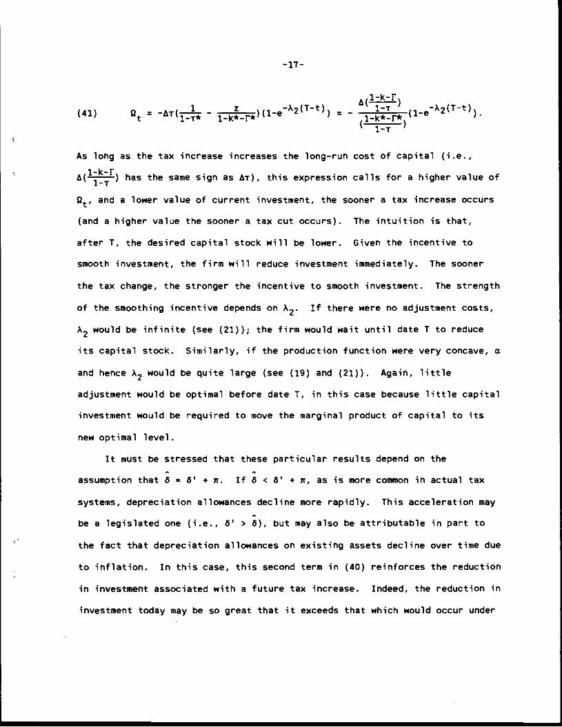
—17—
1-k-F
(41) = -At( 1 - z )(l_e2(T_t)) = - 1T(iflc
2(Tt)t 1-Ta 1-k*-r* 1-k-N
1—1
As long as the tax increase increases the long—run cost of capital (i.e.,
a(1_k_F) has the same sign as at), this expression calls for a higher value of
and a lower value of current investment, the sooner a tax increase occurs
(and a higher value the sooner a tax cut occurs). The intuition is that,
after T, the desired capital stock will be lower. Given the incentive to
smooth investment, the firm will reduce investment immediately. The sooner
the tax change, the stronger the incentive to smooth investment. The strength
of the smoothing incentive depends on A2. If there were no adjustment costs,
A2 would be infinite (see (21)); the firm would wait until date T to reduce
its capital stock. Similarly, if the production function were very concave, a
and hence A2 would be quite large (see (19) and (21)). Again, little
adjustment would be optimal before date T, in this case because little capital
investment would be required to move the marginal product of capital to its
new optimal level.
It must be stressed that these particular results depend on the
assumption that 5 = 6' + it. If & < 6' + it, as is more common in actual tax
systems, depreciation allowances decline more rapidly. This acceleration may
be a legislated one (i.e., 6' > 5), but may also be attributable in part to
the fact that depreciation allowances on existing assets decline over time due
to inflation. In this case, this second term in (40) reinforces the reduction
in investment associated with a future tax increase. Indeed, the reduction in
investment today may be so great that it exceeds that which would occur under

—18-
an immediate increase in i to T* (i.e., I = t). Alternatively, a delayed cut
in r may increase investment more than an immediate one. This possibility was
demonstrated by Abel (1982) for the case of instantaneous tax depreciation
(6' = ),5 but there is a much weaker and more intuitive necessary condition
for the result to hold.
Consider the effect on of an increase in T:
(42) =h1X2e_X2(T t)([ + 1_k*r*C1 + (616))]
- z p+ir+o' (ö'+1t+Ô)(e(A2_(P+7t+ô')(I_t)l }
1k*r* x2—(p+it+a') p+
For a delay in a tax increase to reduce current investment, this derivative
must have the same sign as Ar. At T = t, the second part of (42) equals zero,dQ
so the condition that sgn(—) = sgn(br) is (given the definitions of F and z)
(p+5)(1_k*_r*)1-r*
The intuition for this result is quite simple. At time t, the new
investment's tax base is negative if its gross marginal product of capital is
less than its depreciation allowance. The left—hand side of (43) is the
long-run cost of capital per dollar under the new tax system, to which the
marginal product will eventually converge, while the right-hand side of (43)
is the instantaneous depreciation allowance per dollar. Although the matter
is complicated by the fact that the actual value of F' won't equal the
left—hand side of (43) immediately (because of adjustment costs), the
intuition is that it the underlying tax base is negative just after
investment, then a delay in a tax cut raises taxes and investment.

—19-
For I > t, the second term in (42) is nonzero. For accelerated
depreciation (6' + it > 6), it has the opposite sign of hi, making it less
drlikely that air- will have the same sign as hr. The intuition is that with
accelerated depreciation the tax base will increase, eventually approaching
the entire marginal product of capital. Thus, if j.t and hi have different
signs at I = 0, their signs remain opposite for I > 0.
The following result may also be demonstrated.
dQt-
Proposition: Suppose hr > 0 N 0) and > 0 (c 0) at I = t. If (p46),
IT, and 8* are all nonnegative, and 6' + it > 6, then there exists a finite
value I > t at which is maximized (minimized).
Proof: There are two cases to consider. If A2 > p + it + 6', it is clear that
the second term in brackets in (42) is negative and becomes arbitrarily large
in absolute value as I increases. This must make the entire term in brackets
negative for all T above some critical value. If A2 < p + it + 6', the second
term again is negative and increases in absolute value with I, but is bounded
by the value it approaches asymptotically at I = . At I = , the term in
brackets in (42) equals:
(44) — + 1_kLr*t1 + (°':)(1 +
which has the same sign as
45 - (p÷o)(1_k*_I'*) +A2-(p+6)
(1Tt)
By assumption, A2 c p + it + 6'. From the definition of A2 (in (21)), it is
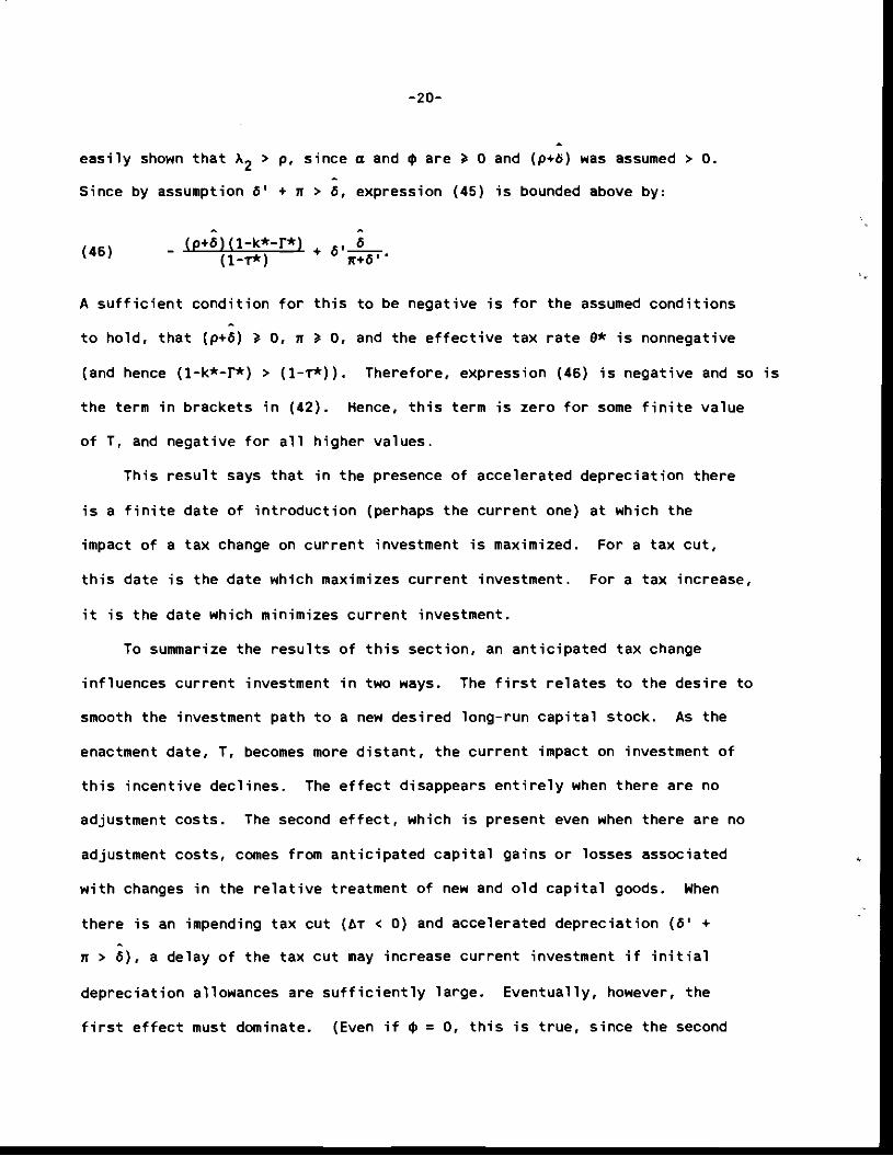
—20—
easily shown that > p. since a and $ are ) 0 and (p÷b) was assumed > o.
Since by assumption 6' + n > 6, expression (45) is bounded above by:
46 — (p+6)(1_k*_r*) + 6'C ) (1_t*)
A sufficient condition for this to be negative is for the assumed conditions
to hold, that (p+6) ) 0, n 0, and the effective tax rate 0* is nonnegative
(and hence (1_k*_r*) (1—r*)). Therefore, expression (46) is negative and so is
the term in brackets in (42). Hence, this term is zero for some finite value
of T, and negative for all higher values.
This result says that in the presence of accelerated depreciation there
is a finite date of introduction (perhaps the current one) at which the
impact of a tax change on current investment is maximized. For a tax cut,
this date is the date which maximizes current investment. For a tax increase,
it is the date which minimizes current investment.
To summarize the results of this section, an anticipated tax change
influences current investment in two ways. The first relates to the desire to
smooth the investment path to a new desired long—run capital stock. As the
enactment date, T, becomes more distant, the current impact on investment of
this incentive declines. The effect disappears entirely when there are no
adjustment costs. The second effect, which is present even when there are no
adjustment costs, comes from anticipated capital gains or losses associated
with changes in the relative treatment of new and old capital goods. When
there is an impending tax cut (fri < 0) and accelerated depreciation (6' +
n > 6), a delay of the tax cut may increase current investment if initial
depreciation allowances are sufficiently large. Eventually, however, the
first effect must dominate. (Even if $ = 0, this is true, since the second

—21—
effect changes sign once assets have been substantially depreciated.)
Considered next are the effects of changes in the investment tax credit,
both temporary and permanent.
B. Anticipated Permanent Chauge in the Investment Tax Credit
Suppose the investment tax credit changes from to k* at date I > t.
Then, for s > I, a = 0 (see (19)). For s c I,
- k*-k - Ak(47) a5 — —
The contribution of this term to is:
(48) x2!Te_x2(T_t)Ir*ds =
Aflkr,=
' 1—t /
tl_e_)2(T_t)1_T*
Comparing (47) and (48) to (35) and (41), one observes that this effect of the
credit is equivalent to that of an anticipated tax cut in the presence of
economic depreciation allowances. A future increase in k leads to more
investment today to smooth the accumulation of the larger capital stock
desired after date T. Just as in the case of accelerated depreciation,
however, there is an additional effect associated with a change in the
relative values of new and old capital. When k increases it decreases the
value of existing capital, which does not qualify for the credit, relative to
new capital, which does. This effect, which discourages current investment if
k is expected to increase, is accounted for by the term appearing in (19).
Because of the jump in k at I, k1 is undefined. Its impact on fl is

—22—
massed at I in a1. However, its effect can be calculated as the limit of the
effects of the Cc terms associated with a change from k to k* over an arbitrarily
short interval around 1. This yields an effect on of:
(49) eA2(Tt) Ak
p+6
which has the same sign as Ak, discouraging investment if Ak > 0. Combining
(48) and (49) yields the total effect of the change in k:
A -(p+6)50 =A,.. , +
2 at2uTtt 1k*•r*' p6
If A2 > (p46), fl exceeds the value it would have for no change in k (i.e.,
for I -, ). In this case, the expectation of an increase in the investment
tax credit reduces current investment. The capital loss effect in (49)
outweighs the smoothing effect in (48). However, A2 may be less than (p+6).
From the definition of A2 in (21), it follows that A2 c (p+5) if and only if
a C When the elasticity of quasirents with respect to changes in the
capital stock, a, is low, and adjustment costs, $, are high, smoothing can
outweigh the capital loss term. As shown below, this is the same condition
for the value of existing capital goods to increase with an increase in the
investment tax credit. The increase indicates that marginal q increases by
more than the gap between marginal and average q does. Since a capital gain
occurs in such an event, the anticipation of such a gain encourages current
investment.
Because 6 depends on $, the condition a c $6 will not be satisfied for
all $ above some critical level. In fact, it will be satisfied for a possibly
—23—
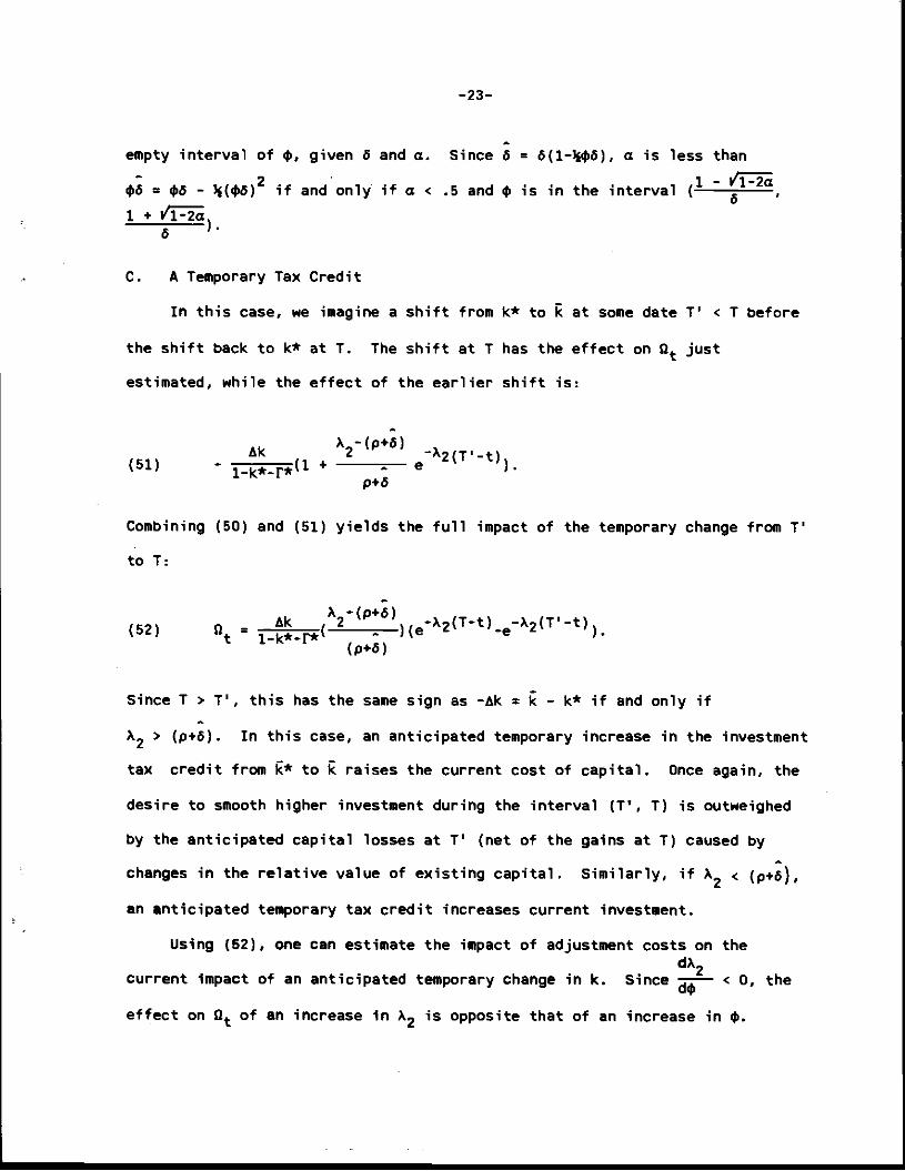
empty interval of $, given 0 and a. Since 6 = 6(1—31*6), a is less than
$6 = - 31(,6)2 if and only if a < .5 and $ is in the interval (1- Y'1-2a
1 + P'1-2aa
C. A Temporary Tax Credit
In this case, we imagine a shift from k* to k at some date V < T before
the shift back to k* at 1. The shift at T has the effect on Q, just
estimated, while the effect of the earlier shift is:
X —(p+6)Ak 2 —X2(T'_t)
(51) — 1_k*_r*' + e
p+6
Combining (50) and (51) yields the full impact of the temporary change from V
to 1:
(52) =
(p+6)
Since I > U, this has the same sign as —Ak = k — k* if and only if
A2> (p+6). In this case, an anticipated temporary increase in the investment
tax credit from k* to raises the current cost of capital. Once again, the
desire to smooth higher investment during the interval (T', 1) is outweighed
by the anticipated capital losses at T' (net of the gains at 1) caused by
changes in the relative value of existing capital. Similarly, if A2 <
an anticipated temporary tax credit increases current investment.
Using (52), one can estimate the impact of adjustment costs on the
dA2current impact of an anticipated temporary change in k. Since
d$< 0, the
effect on of an increase in A2 is opposite that of an increase in $.

—24—
Differentiating (52) with respect to A2, on obtains:
dat _______
dA— —
1—k*-r*
A2(T-t) AATe(AlEX2 — (p+6)] + (e —1)[1 — (T'—t)[A2
— (p+o)])}p+6
where AT = I - 1' > 0. Consider the "normal" case where (p+6) < A2, where an
anticipated credit discourages current investment. For a temporary increase
in k (Ak = k* — k < 0), the expression in (53) is positive if
(V-fl <1
(Otherwise, the two terms in brackets on the right-handA -(p+O)
on the rigt-hand side of (53) are of opposite sign and the overall sign is
ambiguous.) Thus, for a temporary policy that starts sufficiently soon
(T' -. t), an increase in $ (which decreases A2) will reduce fl, thereby
lessening the negative impact on current investment. For a more distant
policy, the inability to adjust quickly to changes in incentives when q is
large is opposed by the greater relevance of future tax changes.
4. Numerical Simulations of Effective Tax Rates
This section uses the expression derived in the last section to
illustrate the effects, 0, on the cost of capital associated with tax reforms
such as those recently enacted in the U.S., and translate these estimates into
the effective tax rates on current investment with expression (29).
Performing these experiments requires values for several economic and
technological parameters. The real discount rate is set at 4 percent, as is
—25—
the inflation rate. For the constant elasticity specification F(K) = AKT, the
parameter a = 1 - 1' (see (18)). Since this production function corresponds to
the Cobb-Douglas function with other factors (such as labor) held constant,
one may view a as the complement of the capital share of gross output. Since
depreciation in the U.S. is typically about 10 percent of GNP, and capital's
share of net income is about one quarter, it is reasonable to set a = .65.
This value of a guarantees that A2 > (p+6), so that an anticipated cut in the
investment tax credit stimulates investment. The remaining technological
parameters, a and •, are varied to estimate the impact of tax changes for
different types of asset under different adjustment cost conditions. Values
of a = .03 and .10 are used to represent structures and equipment, respectively,
and values of $ = .5 and 20 are considered. The latter value of th is much
more consistent with findings in the empirical literature, though there are
arguments one can make suggesting that such estimates may be biased upward.7
Consider a change in r and k such as that recently adopted in the U.S.
under the Tax Reform Act of 1986. The reform lowered the statutory corporate
tax rate from .46 to .34 and repealed the investment tax credit, which had
been .10 for equipment only. Thus, r = .46, r* = .34, k = .10 and k* = 0
in the base simulations for equipment and k = k* = 0 for structures. Tax
depreciation parameters of 6' = .20 for equipment and 6' = .05 for structures
are used to represent the fact that each asset has accelerated depreciation
under both old and new tax systems, relative to the direct measures of
economic depreciation, a.8
The tax reform was enacted after several years of discussion, during
which it became progressively more likely that the reform would occur. In

—26—
recent years before 1985, important changes in investment incentives were
introduced in 1981, 1982 and 1984. In 1981, as well as in 1986, the reform
eventually introduced was discussed and debated for at least two years. Thus,
it is quite important to consider the potential impact of anticipated tax
changes on current investment.
To assess the impact of expectations, we consider permanent transitions
to the new tax system enacted immediately and with prior announcements of
one and five years. The simulation results are given in Table 1, which gives
effective tax rates B based on expression (29). For purposes of comparison,
simulations that consider the impact on equipment of the changes in T and k
alone are also presented. Results for each simulation include the values of
6, the true rate of economic depreciation, -A1, the speed of adjustment,
and A2, the discount factor applied to the terms a5 (s>t) in computing
The impact of the tax changes in the long run is given by the tax rates
under immediate adoption, since there are no anticipated tax changes in these
Dimulations. As has been pointed out by many who analyzed the recent tax
changes, the long—run effective tax rates rise for equipment (when the
investment tax credit is removed) and fall for structures, with both new rates
very close to the statutory tax rate (at least when 6 6). The fact that
0* r* does not, however, deny the presence of accelerated depreciation. It
simply indicates that the acceleration via 6' is roughly offset in present
value by the lack of inflation indexing. Indeed, the measure of acceleration
that matters in the current context is 6' + it, since this is the rate at which
real depreciation allowances decline. Thus, a delay in the tax cut provision
need not by itself increase the current effective tax rate.
—27—
When the tax change is delayed, the short-run results are different. For
structures, the present value of depreciation allowances is small, so the
positive effect of investment due to increased value of depreciation
deductions does not outweigh the negative effect of a reduction in the
long-run cost of capital. When $ = .5, the value of 0 under a five-year
delay nearly equals its value under the old tax system. The change is heavily
discounted due to the rapid speed of adjustment Ut2 = .32). For equipment,
the acceleration of depreciation itself, described in the second set of
simulations, is enough to make a delay in the tax cut increase current
investment and lower the current effective tax rate. This is because the
present value of depreciation allowance, z, is much higher for this more
rapidly depreciating asset. The anticipated removal of the investment tax
credit described in the third set of simulations increases current investment
as firms wish to invest more to take advantage the investment tax credit.
These two effects combined give the announced policy shifts a powerful effect
on current investment.
As has been pointed out elsewhere (Auerbach and Hines, 1986), it is not
necessary that reductions in the effective tax rate associated with a delay in
tax changes also reduce tax revenues. Indeed, the delayed reduction in r
encourages equipment investment while raising revenue. This is because, while
taxes collected on new investment may be reduced (if 5' exceeds the marginal
product of capital), taxes collected on existing assets will be increased by
keeping the higher tax rate.
This abilit9 to increase current investment and revenue at the same time
is another way of presenting the fact that windfalls are being given existing

—28—
assets when the tax rate is cut. Such windfalls have been seen as an
important shortcoming of the tax reform, since if revenue is being held
constant the effective tax rate on new investment rises. However, one must
stop short of characterizing as superior or more efficient policies that
increase current investment without decreasing current tax revenue, since
taxing existing capital may well have an impact on expectations about the
shape of future "reforms." Nevertheless, the short—run impact of tax reforms,
as well as their long-run consequences, should be considered in light of the
frequency with which new provisions have been introduced.
5. Tax Reform and Market Value
Tax changes affect the value of the firm as well as the incentive to
invest. The close relation of these two effects has already been brought out
in showing how anticipated capital gains and losses are incorporated into
current incentives. It is also possible to calculate how tax reforms affect
the value of the firm as a whole, not just investments undertaken at a
specific date.
At any given time, the value of the firm will depend not only on the
capital stock but also on the previous path of capital accumulation, since
depreciation allowances do not follow economic depreciation. This section's
analysis i limited to cases in which previous accumulation has been in a
steady state. Thus, the tax reform experiment is one not only near a steady.
state, but where the steady state has been disturbed.
With a single factor of production, capital, and decreasing returns to
—29-
scale, there are two sources of firm value in the absence of taxes: normal
returns to capital and pure economic profits. As always, it is possible to
reinterpret a decreasing returns technology with one factor as a constant
returns technology with two factors, the second being a fixed factor owned by
the firm that "earns" the economic profits as a factor reward. This is
especially helpful in the current context, for then it is possible to apply the
result of Hayashi (1982), adjusted for taxes by Summers (1981). that the
value of the firm's capital stock per unit equals the marginal cost of new
capital, adjusted for differences in tax attributes. Thus, the firm's value
has two components: this tax-adjusted value of marginal q, multiplied by the
capital stock, plus the discounted value of pure profits. This can be
expressed per unit of capital, yielding a value of average q that includes not
only the tax adjusted value of capital but also the discounted profits per
unit of capital. One can then consider the effects of tax reform on the total
as well as the components, a particularly useful exercise if one wishes to
consider the effects of tax reform on the value of the firm under different
assumptions about whether the firm has any pure profits.
To begin, consider the value of the firm's capital stock. The marginal
price of new capital goods is, from (12) and the definition of q,
q = 1 + •k/K. This capital receives investment credits per unit of kq and
depreciation allowances worth rq, and yield a stream of after-tax quasirents in
the future. Hence, the existing capital stock, K, which has the same future
productivity per unit, must be worth q(1-k-r)K + A, where A is the present
value (in terms of taxes saved) of this capital stock's depreciation
allowance deductions.
—30-
Since it has been assumed that this capital was accumulated in a steady
state, a constant amount of capital, 6K, was purchased at each prior date, at
an average price of (1—1$6). This average cost is relevant for calculating
the total value of depreciation allowances, since allowances are based on
total capital expenditures. Thus, the value of depreciation allowances on
existing capital at the current date, zero, is:
0(64) A = f oK(1_½$5)F(t)dt = oKJ r(t)dt
where r(t) is, as before, the present value of depreciation allowances
remaining for an asset of age -t. If one assumes, as above, that depreciation
allowances are at a constant proportional rate 6' but not indexed, then (54)
may be rewritten:
(55) A = OKJ e(O +1T)tflft =
It follows that the average value of the capital stock is:
(56) qK = q(1-k-r) + A/K = q(1-k-r) +
To simplify expression (56), note that, in the steady state, K = K*, the
optimal capital stock under the steady state's tax system Thus, (24) and
(25) may becombined to yield, at t = 0,
(57) k = (-A1)(K—K*) =
Using (57) and the definition of q, one may rewrite (56) as:
(58) qK (1-k-fl5.) + A1.fll—k-r)Q/a.

—31—
In the steady state, k = k*, F = r*Z, and 0 = 0. Thus, the deviation of
qK from its steady state value at time zero due to an unannounced tax policy
change is:
K K K* 5(59) Sq = q - q =—Ak0
-AT0z(1—5, ) +
Where Ak0 = k0— k* and Ar0 = — r*. This value will reflect both changes
in marginal q (through flu) and changes in the relative valuation of new and
old capital.
Next, consider the impact of tax reform on the discounted value of pure
profits. By construction, these profits equal the after—tax quasirents in
each year in excess of the capital stock's marginal product, or, normalized by
the current capital stock,
(60) qP = jif e_Ptu_TtLEKt) — KtFI(Kt}]dt.
For a small change in tax policy around the steady state, the change in qP at
time zero is:
(61) 5qP = et_ATt[r(K*)_K*F1(K*)] —
where Ar = r — 1*. This has two components, due to the change in the
taxation of existing profits, and the change in profits. Given (7') and the
definition of a in (18) this may also be written:
(62) 5qP + afePt(1_rt)(tK*}dt]
An expression for Kt is obtained by solving the first-order differential

—32—
equation (24), using the initial condition that K0 = K*:
(63) K = eAlt(K* - A1fe'1Kds)
which, iven the definition of K in (25), yields:
K-K* A t(64) = ._fe)1(t_5)u5ds.
Substitution of (64) into (62) yields a solution for nqP in terms of exogenous
parameters alone: -
(65) Aq = 514'*)_ j.fePtzsrdt + x1f eP.t(1_Tt) 1t1(t_a5dsdtr.
Expressions (59) and (65) provide the component changes in market value
resulting from any change in tax policy -initiated at date zero. For immediate,
permanent tax changes q, they simplify considerably.
For a permanent change in k and T, it follows from (40) and (50) that:
(66) £2 E - ______ - Ar(1_r4* - z)]
which is simply the proportional change in the long run cost of capital,
(p+5)(1-k—r)/(1—r). Substituting (65) into (59) and (65) (and using the facts
that A1 + A2 = p and A1A2 = — a(P;5)) yields:
K _______ O(67a) = [Ak — Ar( 1_T*
— z))( - [Ak + Atz(1—51,1)]

—33-
(670) 5qP = (Ak - Sr*T - z))(? - £!) - ATj(14 )(22)]
I k p 6 lk** I p+6 6 6(67c) Sq = Sq + Sq = Sk - kr(( 1-7* j—&—i-
- z(6. +
From these expressions, a number of points about the effects of changes in
r and k may be made. Each tax change affects the value of the capital stock,
qK, in two ways, represented by the two bracketed terms in (67a). The first
is the change due to the change in marginal q, the second the change in the
relative value of new and existing assets. Any policy that increases marginal
q (a cut in t or an increase in k) increases the first term, while with
accelerated depreciation, the credit increase and the tax cut affect the
second term in opposite directions ways. The credit increase causes a capital
loss by increasing the distinction between old and new capital, while the tax
cut narrows the difference associated with differences in prospective
depreciation allowances.
A second difference between the two policies appears in expression (6Th),
the impact on the present value of pure profits. This is due to the extra
windfall given to the firm by a tax cut as the result of the reduced taxation
of existing profits. Since A2 p (for F' and hence p + 6 > 0), policies of
either type that encourage investment also increase profits through an
expansion of output. This profit increase depends on the assumption that the
firm faces fixed output prices. In a more general model, with other factors
of production or profits bid down by declining output prices, one might expect
all or part of this increase in profits to be absent.
The division of changes in the total value of the firm between changes in
the value of capital and changes in the value of profits depends on the

-34-
technology of adjustment. For an investment tax credit, the total change in
the value of the firm is simply the discounted value of additional
investment credits. With high adjustment costs, A2 -. p, so this appears
entirely as an increase in there is little change in output or profits and
the firm simply receives the additional credits as a windfall to capital. At
the other extreme, with no adjustment costs, Aq1 = -Ak, as the value of
marginal q doesn't change at all. At the critical intermediate value of
A2 = p + 6 (where, as shown above, a = •6), the effect on qi( is zero, as the
two effects in (67a) cancel.
For a tax cut, the situation is more complicated, depending on the extent
to which depreciation allowances are accelerated. Total value increases by
more per unit increase in marginal q than in the case of the investment tax
credit for three reasons: reduced taxation of normal returns to existing
capital, reduced taxation of the component of the tax base associated with
recapture of previous accelerated depreciation, and reduced taxation of
preexisting profits. The first two effects are present in (67a), the last in
(67b). Even with no adjustment costs (A2 = ), the value of the capital stock
increases because of the reduced tax on recapture of accelerated depreciation,
aby £rz(1 5P÷)
Since much of the criticism of the recent tax reform has focused on
shifts in the tax burden between new and old capital, it is interesting to
consider the effects on the value of the existing capital stock, qK, of such a
change.
Table 2 presents calculations of based on (67a) for the same permanent
tax reform considered in Table 1, the removal of the 10 percent investment tax

-35-
credit for equipment and a cut in the corporate tax rate from .46 to .34. The
calculations use the same economic parameters as before (5 • .1, 5. = .2 for
equipment, S = .03, 6' = .05 for structures, and p = it = .04). For each
case, the change, in qK is broken down into four components: the changes in
marginal q and the gap between marginal and average q caused by the changes in
k and 7.
As expected, the combined effects coming through marginal q are negative
for equipment and positive for structures, with the effects larger when
adjustment costs are large. This impact of adjustment costs is especially
strong for structures because of the lower rate at which structures
depreciate; existing capital gets the benefit of increased after—tax returns
over a longer period. The "windfall" effects represented by increases in the
value of old relative to new capital are positive for both parts of the
policy, the removal of the tax credit and the reduction in the tax rate. For
equipment, each part of the policy raises the market value of capital, with
the total impact relatively insensitive to the size of adjustment costs. For
structures, the total increase value is substantially higher with higher
adjustment costs.
Given the differences in modelling approaches (analytical linear
approximation versus exact calculations derived from a numerical simulation
model) and economic assuliptions these results are quite consistent with those
found by Auerbach and Hines (1986).

-36-
6. Conclusion
This paper has presented an analytical discussion of the impact of tax
reforms on current investment and market value, taking account not only of the
nature of the tax law but also the production and adjustment cost technology.
Its main contribution has been the derivation of analytical expressions
for the impact of future tax provisions on the value of the firm and the user
cost of capital. These expressions are helpful in understanding the impact of
particular tax changes and the importance of investment smoothing and
announcement effects.
Many important considerations have been omitted from the analysis. For
example, in recent years, tax losses and other constraints have been an
important phenomenon. The impact of such constraints varies across assets and
can either encourage or discourage investment (Auerbach, 1983, 1986; Auerbach
and Poterba, 1986; Altshuler and Auerbach, 1986). In an environment without
perfect loss offset, the effects of immediate or delayed tax reforms may be
quite different than those portrayed here. In considering assets individually,
one ignores the spillover effects that changes in one type of investment may
have on another through complementarity in the production function and shared
adjustment costs. A multiple capital stock model is too complicated for the
derivation of interpretable analytical expressions, although Auerbach and
Hines (1986) have considered the effects of large anticipated tax changes in a
numerical simulation model with two capital stocks.
The analysis has emphasized the important relation between investment
incentives and changes in the firm's market value, both present and

—37—
anticipated. For these to be useful in evaluating tax incentives, a better
positive model of the dynamic process of tax reform is needed.
-38—
Footnotes
1. The expression for taxes in (2) treats all capital costs pKC(I/K)I as
part of capital expenditures for tax purposes. This is consistent with the
U.S. tax treatment calling for the addition of indirect costs (such as
installation) to basis. In reality, some of the indirect costs associated
with adding capital, such as retraining of labor, would normally not be
capitalized but simply deducted as an expense.
2. This latter effect would be absent if adjustment costs depended only on
the level of investment, rather than the ratio of investment to the capital
stock. The ratio specification is typically used in the empirical literature
estimating adjustment costs. An additional reason for using it here is that
it makes analysis of the effects on market value easier. This choice of
specification has some impact on the results concerning investment behavior.
An earlier version of the paper used the level rather than ratio
specification. The differences in results are discussed below.
3. The total cost to the firm of new capital goods is (1—o+igI/K)I =
(1-it$a)&K in the steady state. The steady state value of the firm's capital
stock is constant. Thus, depreciation, which is the reduction in capital
value plus expenditure on new capital goods, is (1-J4iö)6K = 6K. Another way
of viewing the same result is that an increase in capital expenditure today,
holding future expenditure constant, yields an asset that depreciates at rate
o plus additional capital at each date in the future because of the reduced
unit price of capital induced by the current expenditure. The increase (in
the steady state) is per unit of capital, compounded at each date,

p—39—
yielding a net rateof depreciation of o -
As shown by Abel(1982), neutralIty of the tax
system in such a casewould requirenetting these gains
against primarydepreciation in
computingdepreciation allowances.That such a
correction to themeasurement ofeconomic
depreciation isappropriate does not
appear to be widelyrecognizedin discussions
about measuringdepreciation properly.
Given typical estimatedmagnitudes of theproportional adjustment cost parameter •, the
correction maybe quite large.
4. Note that (1),holding I and K
constant, may be rewritten:q(p + +
Thus, for smallchanges one obtains:
C 1—k—F 1—7 1—k—F5.Abel actually
considered the case where onlya fraction of new investmentcould be written
off immediately, so that z A despite the acceleratedwrite-off. Thecrucial issue,
however, is thetiming of the
allowances.6. A similarambiguity was found in a general
equilibrium model withoutadjustment costs, but with the interestrate Influenced
by individualsavingsdecisions by Judd
(1985). Implicit in the fixedinterest rate
assumption madehere is thenotion that that the assets
being considered are smafl relative tothe (perhapsinternational) capital market. The choice
of adjustment costspecification is alsocrucial here. Under the level
adjustment costspecification used in an earlier
paper (C(I) instead of C(I/K)),A2 mustexceed p45 and the ambiguity
disappears. The condition a c p6 say be shownto imply that the reduction inthe marginal
product of existingcapital causedby new investment
is less thanthe increase in
adjustment cost rentsearned bythe same
capital. Such rentsare zero in the
C(I) specification.
-40--
7. For furtherdiscussion, seeAuerbach
and Hines (1986).
8. The law a'so included changes indepreciation provisions
that were less
important thanthe changes in r and Ic
9. Since perterbationsaround the steady
state are being assumed, these
"permanent" changes are,strictly speaking,
temporary changesof a very long
duration.

—41—
References
Abel, A. 1982. "Dynamic Effects of Permanent and Temporary Tax Policies in a
Q Model of Investment, Journal of Monetary Economics (May).
__________ 1983. "Tax Neutrality in the Presence of Adjustment Costs,"
Quarterly Journal of Economics (November).
Altshuler, R. and A.J. Auerbach. 1986. "The Significance of Tax Law Asym-
metries: An Empirical Investigation." Mimeo.
Auerbach, A.J. 1983. "Corporate Taxation in the United States," Brookings
Papers on Economic Activity 2.
_________ 1986. "The Dynamic Effects of Tax Law Asymmetries," Review of
Economic Studies (April).
Auerbach, A.J. and J.R. Hines. 1986. "Tax Reform, Investment, and the Value
of the Firm." NBER Working Paper #1803. Cambridge, Mass.: National
Bureau of Economic Research, January.
Auerbach, A.J. and J.M. Poterba. 1986. "Tax Loss Carryforwards and Corporate
Tax Incentives. NBER Working Paper #1863. Cambridge, Mass.: National
Bureau of Economic Research, March.
Hayashi, F. 1982. "Tobin's Marginal and Average q: A Neoclassical Inter-
pretation," Econometrica (January).
Judd, K. 1985. "Short Run Analysis of Fiscal Policy in a Simple Perfect
Foresight Model," Journal of Political Economy (April).
King, H. and D. Fullerton, eds. 1984. The Taxation of Income from Capital.
Chicago: National Bureau of Economic Research,
—42—
Summers, L. 1981. "Taxation and Investment: A Q Theory Approach," Brookings
Papers on Economic Activity 1.
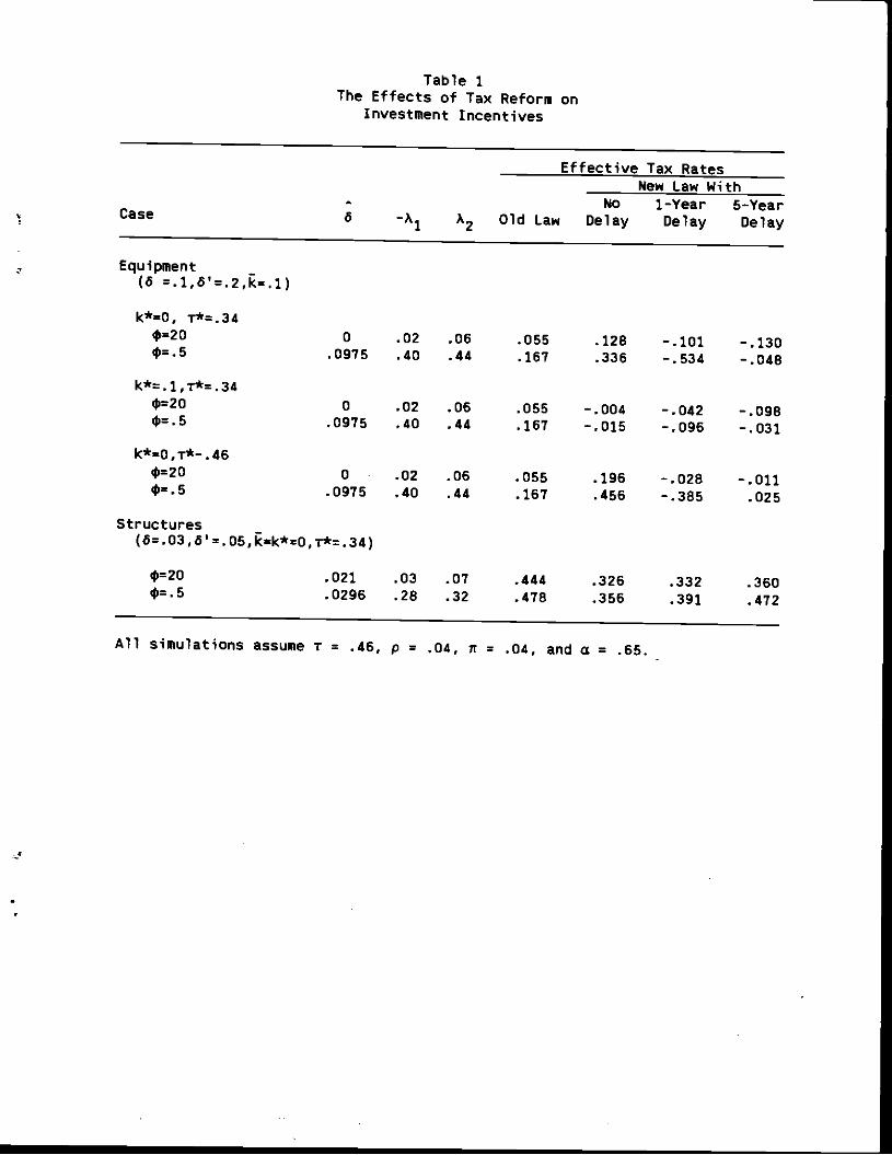
Table 1The Effects of Tax Reform on
Investment Incentives
Case 6-A1 A2
Effective
Old Law
Tax Rates
No
Delay
New Law W1—Year
Delay
ith
5-Year
Delay
Equipment -
(6 =.1,o'=.2,k=1)
k*=O, r*=.34$=20 0
.0915.02
.40.06
.44.055
.167.128.336
—.101—.534
—.130—.048
k*=.1,r*=.34$=20 0
.0975.02
.40.06.44
.055
.167
-.004—.015
-.042—.096
-.098—.031
k*=0,r*_ .46
$=20 0.0915
.02
.40.06
.44.055.167
.196
.456—.028—.385
—.011.025
Structures —(6=.03 ,o' .05,kk*=0,r* .34)
t=20 .021.0296
.03
.28
.07
.32.444
.478.326
.356.332
.391
.360
.472
All simulations assume r = .46, p = .04, It = .04, and a = .65.

Table 2The Effects of Tax Reform on
The Value of Existing Capital
Proportional Change in CapResulting From:
ital Value
Removal of Investment Credit Cut in Corporate Tax Rate
New-Old New-Old
Marginal Capital Overall Marginal Capital Overall
Asset Effect Effect Effect Effect Effect Effect Total
Equipmentcp=2O —.067 .100 .033 .028 .086 .114 .147
•=.s —.032 .100 .068 .013 .051 .064 .132
Structures
$=2O —— —— —— .119 .035 .154 .154
$=.5 -- -- -- .030 .031 .061 .061
Calculations are based on parameters used for simulations presented in Table 1.
Analytically, the effects are defined (based on (67a)) by:
investment credit cut:
marginal: Ak(p+ö)/A2new-old capital: hk
corporate tax cut:
marginal:
new-old capital:
______ - z)(p+ö)1A2
-ATZ(1 -)


