

Non-invasive in vivo measurement of the tear
film using spatial autocorrelation in a live
mammal model
Kaveh Azartash,1 Chyong-jy Nein Shy
2, Kevin Flynn
2, James V. Jester,
2
and Enrico Gratton 1,*
1 Laboratory for Fluorescence Dynamics, University of California, Irvine, Biomedical Engineering Department 3120
Natural Sciences 2 Irvine, CA 92697-2715, USA 2 The Gavin Herbert Eye Institute University of California, Irvine Medical Center 101 the city dr. bldg 55 Orange, CA
92686, USA
Abstract: Tear film stability and its interaction with the corneal surface
play an important role in maintaining ocular surface integrity and quality of
vision. We present a non-invasive technique to quantify the pre-corneal tear
film thickness. A cMOS camera is used to record the interference pattern
produced by the reflections from multiple layers of the tear film Principles
of spatial autocorrelation are applied to extract the frequency of the periodic
patterns in the images. A mathematical model is developed to obtain the
thickness of the tear film from the spatial autocorrelation image. The
technique is validated using micro-fabricated thin parylene films. We
obtained repeatable and precise measurement on a live rabbit model (N = 6).
We obtained an average value of 10.2µm and standard deviation of, SD =
0.3 (N = 4). We measured one rabbit infected with HSV-1 virus that had a
baseline tear film thickness of 4.7µm.
©2010 Optical Society of America
OCIS codes: (170.4470) General; (170.4460) General science
References and Links
1. A. J. Bron, J. M. Tiffany, S. M. Gouveia, N. Yokoi, and L. W. Voon, “Functional aspects of the tear film lipid
layer,” Exp. Eye Res. 78(3), 347–360 (2004).
2. V. J. Forrester, A. D. Dick, P. G. McMenamin, and W. R. Lee, The Eye: Basic Science in Practice (W.B.
Saunders, London, 2002), pp. 447.
3. 2007 report of the International Dry Eye Workshop (DEWS), Ocul. Surf. 5(2), 1–204 (2007).
4. A. Joshi, D. Maurice, and J. R. Paugh, “A new method for determining corneal epithelial barrier to fluorescein in
humans,” Invest. Ophthalmol. Vis. Sci. 37(6), 1008–1016 (1996).
5. H. D. Perry, “Dry eye disease: pathophysiology, classification, and diagnosis,” Am. J. Manag. Care 14(3 Suppl),
S79–S87 (2008).
6. R. Montés-Micó, J. L. Alió, and W. N. Charman, “Dynamic changes in the tear film in dry eyes,” Invest.
Ophthalmol. Vis. Sci. 46(5), 1615–1619 (2005).
7. M. E. Johnson, and P. J. Murphy, “Changes in the tear film and ocular surface from dry eye syndrome,” Prog.
Retin. Eye Res. 23(4), 449–474 (2004).
8. M. A. Lemp, chairman, Report of the National Eye Institute/Industry Workshop on Clinical Trials in Dry Eyes,
CLAO J. 21(4), 221–232(1995).
9. M. A. Lemp, “Advances in understanding and managing dry eye disease,” Am. J. Ophthalmol. 146(3), 350–356,
e1 (2008).
10. M. Ozdemir, and H. Temizdemir, “Age- and gender-related tear function changes in normal population,” Eye
(Lond.) 24(1), 79–83 (2010).
11. C. G. Begley, B. Caffery, K. Nichols, G. L. Mitchell, R. Chalmers; DREI study group, “Results of a dry eye
questionnaire from optometric practices in North America,” Adv. Exp. Med. Biol. 506(Pt B), 1009–1016 (2002).
12. G. U. Kallarackal, E. A. Ansari, N. Amos, J. C. Martin, C. Lane, and J. P. Camilleri, “A comparative study to
assess the clinical use of Fluorescein Meniscus Time (FMT) with Tear Break up Time (TBUT) and Schirmer’s
tests (ST) in the diagnosis of dry eyes,” Eye (Lond.) 16(5), 594–600 (2002).
#131805 - $15.00 USD Received 19 Jul 2010; revised 3 Oct 2010; accepted 7 Oct 2010; published 8 Oct 2010(C) 2010 OSA 1 November 2010 / Vol. 1, No. 4 / BIOMEDICAL OPTICS EXPRESS 1127

13. J. Németh, B. Erdélyi, B. Csákány, P. Gáspár, A. Soumelidis, F. Kahlesz, and Z. Lang, “High-speed
videotopographic measurement of tear film build-up time,” Invest. Ophthalmol. Vis. Sci. 43(6), 1783–1790
(2002).
14. P. E. King-Smith, B. A. Fink, R. M. Hill, K. W. Koelling, and J. M. Tiffany, “The thickness of the tear film,” in
Current Eye Research (Informa Healthcare: London, 2004), pp. 357–368.
15. P. E. King-Smith, B. A. Fink, N. Fogt, K. K. Nichols, R. M. Hill, and G. S. Wilson, “The thickness of the human
precorneal tear film: evidence from reflection spectra,” Invest. Ophthalmol. Vis. Sci. 41(11), 3348–3359 (2000).
16. J. J. Nichols, and P. E. King-Smith, “Thickness of the pre- and post-contact lens tear film measured in vivo by
interferometry,” Invest. Ophthalmol. Vis. Sci. 44(1), 68–77 (2003).
17. P. E. King-Smith, B. A. Fink, and N. Fogt, “Three interferometric methods for measuring the thickness of layers
of the tear film,” Optom. Vis. Sci. 76(1), 19–32 (1999).
18. T. J. Licznerski, H. T. Kasprzak, and W. Kowalik, “Analysis of Shearing Interferograms of Tear Film Using Fast
Fourier Transforms,” J. Biomed. Opt. 3(1), 32–37 (1998).
19. D. H. Szczesna, and H. T. Kasprzak, “Numerical analysis of interferograms for evaluation of tear film build-up
time,” Ophthalmic Physiol. Opt. 29(3), 211–218 (2009).
20. D. H. Szczesna, H. T. Kasprzak, J. Jaronski, A. Rydz, and U. Stenevi, “An interferometric method for the
dynamic evaluation of the tear film,” Acta Ophthalmol. Scand. 85(2), 202–208 (2007).
21. K. Y. Li, and G. Yoon, “Changes in aberrations and retinal image quality due to tear film dynamics,” Opt.
Express 14(25), 12552–12559 (2006).
22. D. Huang, E. A. Swanson, C. P. Lin, J. S. Schuman, W. G. Stinson, W. Chang, M. R. Hee, T. Flotte, K. Gregory,
C. A. Puliafito, and et, “Optical coherence tomography,” Science 254(5035), 1178–1181 (1991).
23. J. Wang, D. Fonn, T. L. Simpson, and L. Jones, “Precorneal and pre- and postlens tear film thickness measured
indirectly with optical coherence tomography,” Invest. Ophthalmol. Vis. Sci. 44(6), 2524–2528 (2003).
24. ANSI Z136, 1–2007, A.N.S.f.S.U.o. Lasers, editor (Laser Institute of America, 2007).
25. N. O. Petersen, “Scanning fluorescence correlation spectroscopy. I. Theory and simulation of aggregation
measurements,” Biophys. J. 49(4), 809–815 (1986).
26. P. W. Wiseman, and N. O. Petersen, “Image correlation spectroscopy. II. Optimization for ultrasensitive
detection of preexisting platelet-derived growth factor-beta receptor oligomers on intact cells,” Biophys. J. 76(2),
963–977 (1999).
27. A. Arduini, M. J. vande Ven, S. B. Shohet, G. Mancinelli, and E. Gratton, “Measurement and analysis of triplet-
state lifetimes by multifrequency cross-correlation phase and modulation phosphorimetry,” Anal. Biochem.
195(2), 327–329 (1991).
28. Covindjee, M. Van de Ven, J. Cao, C. Roye, and E. Gratton, “Multifrequency cross-correlation phase
fluorometry of chlorophyll a fluorescence in thylakoid and PSII-enriched membranes,” Photochem. Photobiol.
58(3), 438–445 (1993).
29. K. M. Berland, P. T. C. So, and E. Gratton, “Two-photon fluorescence correlation spectroscopy: method and
application to the intracellular environment,” Biophys. J. 68(2), 694–701 (1995).
30. M. A. Digman, and E. Gratton, “Imaging barriers to diffusion by pair correlation functions,” Biophys. J. 97(2),
665–673 (2009).
31. N. O. Petersen, “Scanning fluorescence correlation spectroscopy. I. Theory and simulation of aggregation
measurements,” Biophys. J. 49(4), 809–815 (1986).
32. M. A. Digman, C. M. Brown, P. Sengupta, P. W. Wiseman, A. R. Horwitz, and E. Gratton, “Measuring fast
dynamics in solutions and cells with a laser scanning microscope,” Biophys. J. 89(2), 1317–1327 (2005).
33. E. Gielen, N. Smisdom, M. vandeVen, B. De Clercq, E. Gratton, M. Digman, J. M. Rigo, J. Hofkens, Y.
Engelborghs, and M. Ameloot, “Measuring diffusion of lipid-like probes in artificial and natural membranes by
raster image correlation spectroscopy (RICS): use of a commercial laser-scanning microscope with analog
detection,” Langmuir 25(9), 5209–5218 (2009).
34. M. A. Digman, and E. Gratton, “Analysis of diffusion and binding in cells using the RICS approach,” Microsc.
Res. Tech. 72(4), 323–332 (2009).
35. M. Vendelin, and R. Birkedal, “Anisotropic diffusion of fluorescently labeled ATP in rat cardiomyocytes
determined by raster image correlation spectroscopy,” Am. J. Physiol. Cell Physiol. 295(5), C1302–C1315
(2008).
36. E. Gielen, N. Smisdom, B. De Clercq, M. vandeVen, R. Gijsbers, Z. Debyser, J.-M. Rigo, J. Hofkens, Y.
Engelborghs, and M. Ameloot, “Diffusion of myelin oligodendrocyte glycoprotein in living OLN-93 cells
investigated by raster-scanning image correlation spectroscopy (RICS),” J. Fluoresc. 18(5), 813–819 (2008).
37. D. L. Kolin, and P. W. Wiseman, “Advances in image correlation spectroscopy: measuring number densities,
aggregation states, and dynamics of fluorescently labeled macromolecules in cells,” Cell Biochem. Biophys.
49(3), 141–164 (2007).
38. S. Kukreti, A. Cerussi, B. Tromberg, and E. Gratton, “Intrinsic near-infrared spectroscopic markers of breast
tumors,” Dis. Markers 25(6), 281–290 (2008).
39. R. Machorro, L. E. Regalado, and J. M. Siqueiros, “Optical properties of parylene and its use as substrate in beam
splitters,” Appl. Opt. 30(19), 2778–2781 (1991).
40. D. Dursun, D. Monroy, R. Knighton, T. Tervo, M. Vesaluoma, K. Carraway, W. Feuer, and S. C. Pflugfelder,
“The effects of experimental tear film removal on corneal surface regularity and barrier function,”
Ophthalmology 107(9), 1754–1760 (2000).
#131805 - $15.00 USD Received 19 Jul 2010; revised 3 Oct 2010; accepted 7 Oct 2010; published 8 Oct 2010(C) 2010 OSA 1 November 2010 / Vol. 1, No. 4 / BIOMEDICAL OPTICS EXPRESS 1128
1. Introduction
The pre-corneal tear film in mammals is defined as the outermost layer in the eye. Tear film
protects the surface of the cornea and conjunctiva from dust, debris and toxic skin lipids [1].
Additionally tear film provides lubrication for the ocular surface [2,3]. Tear film thickness can
reveal information on the dynamics and physiology of tear layer [4]. Tear film thickness is
also demonstrably related to dry eye syndrome (DES) [5,6]. DES consists of a diverse group
of ocular surface disorders with multiple etiologies [7]. The common characteristic of DES is
an abnormal tear film with inadequate ocular lubrication due to tear deficiency or excessive
tear evaporation [8]. It is believed that dry eye is one of the most common ocular problems in
the United States with a prevalence that goes up to 30% [9], which generally increases with
aging and can impact quality of life [10]. Symptoms include irritation and pain caused by
ocular dryness, among others [11]. The tear film is composed of three layers: the external lipid
layer, an aqueous layer and an internal mucin layer [9]. Therefore, an accurate measurement
of the tear film thickness could provide a method to diagnose dysfunctions in the production
and maintenance of the tear film. A simple thickness measurement could be crucial for
predicting the behavior and stability of the tear film [7].
Tear film thickness is clinically diagnosed by the Schirmer Test, which measures aqueous
tear volume, and the tear Break Up Time (tBUT), which detects the time for the tear layer to
become unstable. Tests based on fluorometry, such as 1% fluorescein and the principle of tear
dilution, have been used as an alternative method to measure aqueous tear production [12].
Amongst the non-invasive techniques, high-speed videokeratography has been applied to
measure the tear film build-up time [13]. Additionally, wavefront aberrometry has been used
to quantify the tear break-up time (tBUT) [6]. Interferometry has also been applied to
measuring the thickness of the tear film. There are two different interferometry techniques
which have been proposed and applied in ophthalmic research. King-Smith et al were
amongst the pioneers in applying interferometry to evaluating and characterizing the tear film.
Their approach analyzed the reflectance spectra from the tear film using visible and near-
infrared light sources, assessing the modulation and phase of the oscillations in the reflection
spectra. They were able to quantify the thickness of the pre-corneal tear film and obtained a
value of 3 µm [14–17]. Licznerski et al applied a modified lateral shearing interferometry
(LSI) and developed a platform for scientists and researchers to characterize tear film
thickness [18]. This method was mainly applied by Szczesna et al to evaluate the dynamics of
the tear film. They were able to assess the stability of the tear film on the ocular surface and
also contact lenses. In this method, interference patterns are captured by means of a CCD
camera. These fringes undergo a Fourier transformation to analyze the changes in their
orientation in the interferograms. They managed to obtain quantitative information on tear
layer applying the bases of Fourier transformation [19,20]. In other works, Li et al applied a
Shack-Hartmann wavefront sensor to non-invasively characterize the tear film topography
[21].
Optical coherence tomography (OCT) has also been used to measure tear film thickness.
OCT is a non-invasive cross-sectional imaging methodology used in biomedical applications.
A low coherence light source is used in OCT systems to obtain a two dimensional image that
could reveal optical characteristics of the specimen [22]. Wang et al used a commercial OCT
system to indirectly measure the thickness of the normal pre-corneal tear film [23].
The technique presented in this article, Fluctuation Analysis by Spatial Image Correlation
(FASIC), is a novel and non-invasive method for evaluating the thickness and spatial features
of the tear film by applying the principles of auto-correlation analysis. A mathematical model
has been developed to translate the spatial fluctuations into thickness information. Extensive
calibration has been performed to validate the system. Animal study has also been conducted.
We show that by calculating spatial autocorrelation in the raw camera images and extracting
#131805 - $15.00 USD Received 19 Jul 2010; revised 3 Oct 2010; accepted 7 Oct 2010; published 8 Oct 2010(C) 2010 OSA 1 November 2010 / Vol. 1, No. 4 / BIOMEDICAL OPTICS EXPRESS 1129

the frequency of the periodic patterns, the average size of the features of tear film can be
obtained.
2 Materials and Methods
2.1 Instrumentation
A schematic of the FASIC setup is shown in Fig. 1. In this setup a 635nm CW-diode laser
(LXC6351AH, Lasermate, Pomona, CA), with less than 1mw in power (0.7 - 0.9mW), was
used as a monochromatic coherent light source. The wavelength and power of this light source
are in compliance with ANSI-2007 standards for laser safety [24]. The laser beam was shone
onto the inferior cornea for animal subjects. The illuminated beam was not focused to a point
and had a collimated diameter of approximately 2mm on the cornea. Therefore the
measurements presented in this dissertation represent the thickness of the pre-corneal tear film
in the region which was covered by the light source.
A cMOS camera (PL-A662-KIT, Pixelink, Ottawa, ON K1G 6C2) was used as means of
capturing the reflection and scattering from the ocular surface. There was an objective lens
(Mitutoyo Compact CF 1X Objective, Edmund Optics, NJ, USA) connected to the cMOS
camera in order to capture an image. This lens was connected to the cMOS camera through an
extender tube. The length of the extender tube was 15cm. The camera assembly was 6.7cm
away from the ocular surface. This distance was the working distance of the objective lens and
was set consistently throughout the animal study to avoid any discrepancy which the focus
could introduce to the data. A stack of 256X256 pixel images was streamed to a computer
through a Firewire cable. The exposure time was set at 1ms and images were acquired at
approximately 300 frames per second. For most experiments, 1000 frames were collected for
a total acquisition time of approximately 3.5 seconds. The incident angle was approximately
10 degrees. The incident angle plays an important role in obtaining the true thickness value
which will be discussed later. The camera angle was slightly greater than the incident angle in
our setup (approximately 12 degrees) to avoid getting specular reflection
Fig. 1. The schematic of the FASIC setup is shown here. A 635nm low power (<1mw) laser is
illuminated onto the cornea in order to measure the pre-corneal tear film thickness. The
reflecting and scattering light is captured by a cMOS camera that is positioned in an angle with
respect to the incoming light. A stack of 256X256 pixel images are streamed to a computer
through a firewire cable for further analysis.
2.2 Spatial Autocorrelation and Physical Principles
Spatial autocorrelation is a statistical analysis that measures and evaluates the degree of
dependency and similarity of a set of data with itself. Petersen et al [25] introduced the
#131805 - $15.00 USD Received 19 Jul 2010; revised 3 Oct 2010; accepted 7 Oct 2010; published 8 Oct 2010(C) 2010 OSA 1 November 2010 / Vol. 1, No. 4 / BIOMEDICAL OPTICS EXPRESS 1130

concept of spatial correlation to the imaging and microscopy community for applications in
fluorescence correlation spectroscopy. This analysis was later improved by Wiseman-Petersen
by introducing other applications for the image correlation spectroscopy [26]. Gratton et al established additional applications of the spatial and temporal image correlation analysis, such
as cross and pair correlation analysis [27–30].
In this work, the specific characteristics of spatial autocorrelation are used to obtain
quantitative information on the dynamics of pre-corneal tear film. The spatial autocorrelation
relationship is given by [31]:
1
),(
),(),(),(
2
,
,
yx
yxs
yxI
yxIyxIG
(1)
where I(x,y) represent the image intensity, ξ and ψ are the spatial increments in the x and y
directions, respectively, and the angle bracket indicates the average over all of the spatial
locations in both x and y directions. In this technique, the spatial autocorrelation analysis is
performed on a 2-D camera image which contains interference patterns from different sources,
along with other features such as dots and lines with various sizes and orientations. These
features in the camera image are difficult to distinguish using the human eye alone. By
transferring the data into frequency domain, these features are more differentiable. Digman et al [32] introduced Raster Image Correlation Spectroscopy (RICS) where they identified and
characterized the dynamics of cell motion through correlation analysis. RICS has been widely
adapted by biologists and experimentalists throughout the world [33–37].
The mathematical operation of spatial autocorrelation works by shifting an image in both
the x and y directions by one pixel and multiplying it by itself. This routine is performed for
half the size of the image, since there is symmetry in the spatial autocorrelation image. This
process is time consuming however, and could be numerically intensive. In order to expedite
the spatial autocorrelation calculations, Fourier transformation is applied. To perform the
spatial autocorrelation analysis with Fourier transformation, the raw camera image first
undergoes a 2-D transformation. The complex conjugate of this image is then calculated and
multiplied by the original transformed image producing a power spectrum. In order to better
visualize the features in the frequency domain, the inverse of the power spectrum is
calculated. This process is fast and robust.
Upon light illumination and provided the specific geometry described above, a periodic
pattern is formed at the ocular surface and is captured by the camera detector (Fig. 2a). This
pattern originates from interference between multiple layers ofe tear film. The reflection at the
inner surface of the tear film produces a slight rotation or displacement of the system of
wavefronts. Superimposed to this pattern, there are many features such as lines and rings and
other structures generated by scattering centers at the surface and, possibly the heterogeneity
of the surface itself.
The spatial autocorrelation function and analysis processes, such as applying a high-pass
filter, act as a filter to select the specific periodic patterns which correspond to the thickness of
a thin film. The spatial correlation image (SCI) also known as autocorrelation function,
contains the average shapes and sizes of the raw camera image (Fig. 2b). For example, if the
image is made of randomly placed features, the SCI, which represents the average shape and
size, is equal to the weighted average of the shape and size of each individual feature. If the
average image is made of circular and linear fringes, such as in an interference pattern, the
SCI will represent the average periodic shape of the fringes. Specifically, the spatial
correlation calculation provides the average features of the image, disregarding their specific
location in the image.
As a consequence of complexity of the spatial features of the illumination pattern,
scattering centers, and other imperfections, the pattern may only be analyzed using the
#131805 - $15.00 USD Received 19 Jul 2010; revised 3 Oct 2010; accepted 7 Oct 2010; published 8 Oct 2010(C) 2010 OSA 1 November 2010 / Vol. 1, No. 4 / BIOMEDICAL OPTICS EXPRESS 1131
autocorrelation function and after selecting the unperturbed periodic pattern. The periodic
pattern is in general complex, although it follows the basic dependency on the tear film
thickness. The factors affecting the periodic part of the spatial autocorrelation function have
been experimentally determined through calibration using standard blocks. We show that the
period of the pattern depends on the inverse of the thickness of the film.
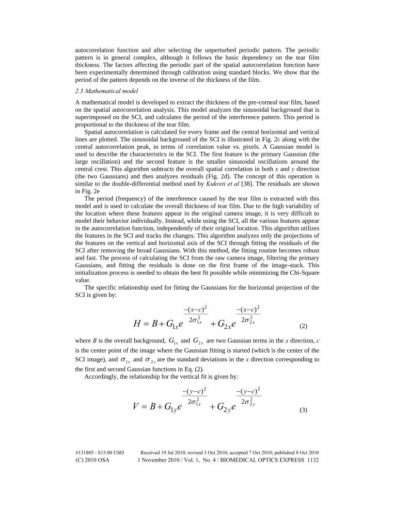
2.3 Mathematical model
A mathematical model is developed to extract the thickness of the pre-corneal tear film, based
on the spatial autocorrelation analysis. This model analyzes the sinusoidal background that is
superimposed on the SCI, and calculates the period of the interference pattern. This period is
proportional to the thickness of the tear film.
Spatial autocorrelation is calculated for every frame and the central horizontal and vertical
lines are plotted. The sinusoidal background of the SCI is illustrated in Fig. 2c along with the
central autocorrelation peak, in terms of correlation value vs. pixels. A Gaussian model is
used to describe the characteristics in the SCI. The first feature is the primary Gaussian (the
large oscillation) and the second feature is the smaller sinusoidal oscillations around the
central crest. This algorithm subtracts the overall spatial correlation in both x and y direction
(the two Gaussians) and then analyzes residuals (Fig. 2d). The concept of this operation is
similar to the double-differential method used by Kukreti et al [38]. The residuals are shown
in Fig. 2e
The period (frequency) of the interference caused by the tear film is extracted with this
model and is used to calculate the overall thickness of tear film. Due to the high variability of
the location where these features appear in the original camera image, it is very difficult to
model their behavior individually. Instead, while using the SCI, all the various features appear
in the autocorrelation function, independently of their original location. This algorithm utilizes
the features in the SCI and tracks the changes. This algorithm analyzes only the projections of
the features on the vertical and horizontal axis of the SCI through fitting the residuals of the
SCI after removing the broad Gaussians. With this method, the fitting routine becomes robust
and fast. The process of calculating the SCI from the raw camera image, filtering the primary
Gaussians, and fitting the residuals is done on the first frame of the image-stack. This
initialization process is needed to obtain the best fit possible while minimizing the Chi-Square
value.
The specific relationship used for fitting the Gaussians for the horizontal projection of the
SCI is given by:
22
2
21
2
2
)(
22
)(
1xx
cx
x
cx
x eGeGBH
(2)
where B is the overall background, xG1 and xG2 are two Gaussian terms in the x direction, c
is the center point of the image where the Gaussian fitting is started (which is the center of the
SCI image), and x1 and x2 are the standard deviations in the x direction corresponding to
the first and second Gaussian functions in Eq. (2).
Accordingly, the relationship for the vertical fit is given by:
22
2
21
2
2
)(
2
2
)(
1yy
cy
y
cy
y eGeGBV
(3)
#131805 - $15.00 USD Received 19 Jul 2010; revised 3 Oct 2010; accepted 7 Oct 2010; published 8 Oct 2010(C) 2010 OSA 1 November 2010 / Vol. 1, No. 4 / BIOMEDICAL OPTICS EXPRESS 1132
where B is the overall background, yG1 and yG2 are two Gaussian terms in the y direction,
and c is the center point of the image, which is known.
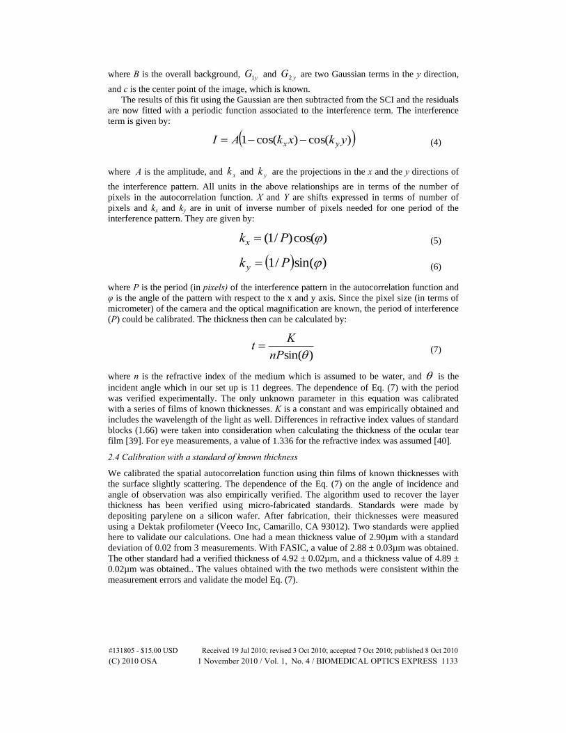
The results of this fit using the Gaussian are then subtracted from the SCI and the residuals
are now fitted with a periodic function associated to the interference term. The interference
term is given by:
)cos()cos(1 ykxkAI yx (4)
where A is the amplitude, and xk and yk are the projections in the x and the y directions of
the interference pattern. All units in the above relationships are in terms of the number of
pixels in the autocorrelation function. X and Y are shifts expressed in terms of number of
pixels and kx and ky are in unit of inverse number of pixels needed for one period of the
interference pattern. They are given by:
)cos()/1( Pkx (5)
)sin(/1 Pky (6)
where P is the period (in pixels) of the interference pattern in the autocorrelation function and
φ is the angle of the pattern with respect to the x and y axis. Since the pixel size (in terms of
micrometer) of the camera and the optical magnification are known, the period of interference
(P) could be calibrated. The thickness then can be calculated by:
)sin(nP
Kt (7)
where n is the refractive index of the medium which is assumed to be water, and is the
incident angle which in our set up is 11 degrees. The dependence of Eq. (7) with the period
was verified experimentally. The only unknown parameter in this equation was calibrated
with a series of films of known thicknesses. K is a constant and was empirically obtained and
includes the wavelength of the light as well. Differences in refractive index values of standard
blocks (1.66) were taken into consideration when calculating the thickness of the ocular tear
film [39]. For eye measurements, a value of 1.336 for the refractive index was assumed [40].
2.4 Calibration with a standard of known thickness
We calibrated the spatial autocorrelation function using thin films of known thicknesses with
the surface slightly scattering. The dependence of the Eq. (7) on the angle of incidence and
angle of observation was also empirically verified. The algorithm used to recover the layer
thickness has been verified using micro-fabricated standards. Standards were made by
depositing parylene on a silicon wafer. After fabrication, their thicknesses were measured
using a Dektak profilometer (Veeco Inc, Camarillo, CA 93012). Two standards were applied
here to validate our calculations. One had a mean thickness value of 2.90µm with a standard
deviation of 0.02 from 3 measurements. With FASIC, a value of 2.88 ± 0.03µm was obtained.
The other standard had a verified thickness of 4.92 ± 0.02µm, and a thickness value of 4.89 ±
0.02µm was obtained.. The values obtained with the two methods were consistent within the
measurement errors and validate the model Eq. (7).
#131805 - $15.00 USD Received 19 Jul 2010; revised 3 Oct 2010; accepted 7 Oct 2010; published 8 Oct 2010(C) 2010 OSA 1 November 2010 / Vol. 1, No. 4 / BIOMEDICAL OPTICS EXPRESS 1133

Fig. 2. (a): Raw camera Image. This image displays the raw camera image from a rabbit’s eye.
This image displays the circular interference pattern caused by tear film layers along with other
features such as: small and large dots with different orientations. This image is one of 1000
time-integrated frames that are captured by the cMOS camera to analyze the spatial
fluctuations. (b): SCI.This image displays the calculated spatial correlation image (SCI) on a
single frame. The SCI has a central peak and a sinusoidal background. The sinusoidal residues
that are located around the peak of the SCI are later used to obtain the quantitative tear film
thickness information. (c). Vertical and horizontal projection of the SCI. This image is
displaying the SCI in terms of number of pixels vs. the correlation value. This image contains
the Gaussian terms along with the residues for both vertical and horizontal axis of two-
dimensional image. The width of the pixels is illustrated on the x-axis while the correlation
value (e.g., number of dots/average intensity of image) is on the y-axis. (d): Preliminary
Gaussian fits in SCI. The SCI undergoes a preliminary fit to remove the primary Gaussian
components. (e): Vertical and Horizontal Fitting. After removal of the Gaussian components,
the sinusoidal residues are fitted both vertically and horizontally for all the frames. This process
provides the period of the interference pattern due to the tear film. After the period of the
interference is obtained, it gets calibrated based on the magnification and true pixel size and is
later used to obtain the true thickness value of the tear film.
3. Results and Discussion
3.1 Live rabbit measurement protocol
Experiments were performed on a live rabbit model. The rabbits were provided by and imaged
at the University of California, Irvine, Medical Center. All procedures were approved by the
UCI IACUC and conducted in accordance with the ARVO Statement for the Humane Use of
Animals in Ophthalmic and Vision Research. Rabbits were anesthetized with intramuscular
injection of xylazine (5mg/Kg) (Anased, Lloyd Laboratories, Shenandoah, IA) and ketamine
(22mg/Kg) (Bionichepharma USA LLC, Lake Forest, IL). Tetracaine hydrochloride 0.5% eye
Drops (Alcon Laboratories Inc, Forth Worth, TX) were instilled into the right eye of each
subject, and a speculum was used to open the eyelids. The laser beam, was angled
approximately 20 degrees with respect to the detecting camera, and was pointed at the inferior
cornea. The camera was placed at about 6.7cm away from the surface of the eye. This is
approximately the focal length of the 1X microscope objective.
For the rabbits with healthy eyes (N = 3), a total of 9 experiments were conducted. Each
rabbit was measured 3 times. Measurements for each rabbit were performed in one day. For
each measurement 1000 frames were captured at approximately 300 frames per second, with
#131805 - $15.00 USD Received 19 Jul 2010; revised 3 Oct 2010; accepted 7 Oct 2010; published 8 Oct 2010(C) 2010 OSA 1 November 2010 / Vol. 1, No. 4 / BIOMEDICAL OPTICS EXPRESS 1134

an overall data acquisition time of approximately 3.3 seconds. A 30-second gap was enforced
between each measurement in order to observe the thinning phenomena of tear film.
3.2 Live rabbit eye measurements
As illustrated in Fig. 3, healthy rabbit #1 had tear film thicknesses of 9.9µm, 9.7µm and
9.6µm in 3 consecutive measurements. Healthy rabbit #2 came out with 10.5µm, 10.4µm and
10.1µm. Healthy rabbit #3 showed tear film thickness values of 10.3µm, 10.1µm and 9.8µm.
The tear film thickness of a rabbit infected with ocular herpes (HSV-1) was also measured.
The measurements for that rabbit were 4.7μm, 4.3µm and 4.1µm. In all 12 measurements, it
was observed that the thickness of the tear film decreases over time. Overall, the baseline
value for the thickness of a healthy rabbit tear film was quantified to be 10.2 ± 0.3. In this set
of experiments, not only the thickness of pre-corneal tear film was precisely quantified, but
also the thinning of the tear film over time was observed.
4
5
6
7
8
9
10
11
Th
ickn
ess(u
m)
He
alth
y
Ra
bb
it #
1
He
alth
y
Ra
bb
it #
2
He
alth
y
Ra
bb
it #
3
Ra
bb
it w
/
Ocu
lar
He
rpe
s
Condition
Fig. 3. Thickness values of the pre-corneal tear films of four rabbits is shown here. Rabbits
were measured at different days and each rabbit has undergone 3 consecutive measurements
with 30 seconds interval at the day of the measurement. Thinning out phenomena is clearly
observed in all animals. Three healthy rabbits have normal tear film thickness of 10.1μm on
average. The one rabbit with ocular herpes had a tear film thickness of 4.7µm and 4.3µm and
4.1µm in the three measurements, respectively.
Figure 4 demonstrates continuous monitoring of the tear thickness during administration
of an artificial tear solution. In this experiment the eyelids were kept open for 1 minute prior
to data acquisition, resulting in a dry eye. At this stage tear film thickness is shown to be
approximately 5μm. At frame 350, about 1.2 seconds into the measurement, a drop of Refresh
Tears ® (Allergan, Irvine, CA) was instilled onto the cornea. A 10-fold increase in thickness
was observed in the tear film, peaking at about 50μm. The tear remains thick for about two
seconds, which is the time required for the drop to travel through the imaging plane. After the
drop expands and the product distributes more uniformly, the tear film maintains a stable
#131805 - $15.00 USD Received 19 Jul 2010; revised 3 Oct 2010; accepted 7 Oct 2010; published 8 Oct 2010(C) 2010 OSA 1 November 2010 / Vol. 1, No. 4 / BIOMEDICAL OPTICS EXPRESS 1135

thickness of approximately 18μm on average throughout the measurement. Figure 4
demonstrates the ability of this technique for real-time assessment of tear film thickness.
Fig. 4. Real time analysis of tear film dynamics in response to instillation of Refresh Tears ®
(Allergan, Irvine,CA). The camera acquired images at 300 frames/s. Changes of the thickness
of tear film over approximately 7 seconds are displayed here. The experiment starts out with a
dried eye. A few seconds into the data acquisition, a drop of Refresh Tear Plus® is instilled
into the rabbit eye. The thickness of the tear film increases approximately 10 fold. After
another two seconds (when the bulk of the drop is out of the imaging plane), the tear film starts
finding a stability in thickness. At this point, the thickness stays at approximately 18µm, and
holds this thickness throughout the data acquisition.
Next, the retention time of the same eye drop (Refresh Tears®) was studied using a live
rabbit model with healthy eyes. As Fig. 5 demonstrates, the original baseline for the subject
was approximately 9.6μm. This value is similar to that obtained previously. After baseline
measurement a drop of 20μl Refresh Tears® was instilled onto the rabbit’s eye. The eye was
manually blinked 3 times so that the eye drop could evenly distribute throughout the ocular
surface. Twenty consecutive measurements were taken with a two-minute gap between each
measurement. As the rabbit was sedated, its eye was manually blinked at 30 second intervals
to prevent evaporation of the eye drop. A peak value of 17.4μm in the first measurement (time
= 0) was obtained. This value was also comparable to values obtained in our previous
measurement with Refresh Tears ®. The thickness maintained values of above 16μm for the
first 5 measurements that were obtained within 10 minutes of eye drop instillation. Sixteen
minutes into the measurement, a more aggressive decline in the value of the tear film
thickness was observed as the pre-corneal tear film thickness decreased to 14.7µm. From the
10th measurement through the 15th measurement, a steady decrease in the thickness values
was observed. In that time frame, the tear film thickness went from 13.8μm to 11.5μm. At
measurement = 16, 32 minutes after the instillation of the drop, the tear film thickness
experienced the sharpest decline in the tear film thickness, as the value returned to 9.8μm. In
the last two measurements, the thickness was similar to the baseline value of 9.6μm. Therefore
the drop retention time was estimated to be about 36 minutes. This set of experiments showed
that FASIC is capable of quantifying the retention time of an artificial tear solution in an
accurate manner.
#131805 - $15.00 USD Received 19 Jul 2010; revised 3 Oct 2010; accepted 7 Oct 2010; published 8 Oct 2010(C) 2010 OSA 1 November 2010 / Vol. 1, No. 4 / BIOMEDICAL OPTICS EXPRESS 1136

Fig. 5. In this figure, the retention time of Refresh Tears® (Allergan, Irvine,CA) was analyzed
using a live rabbit model. The baseline showed a value of 9.6 µm. After the eye drop was
instilled onto the eye, the tear film thickness increased and had a value of 17.4 µm We obtained
a peak value of 17.4μm in the first measurement (time = 0). 10 minutes into the measurement,
the thickness maintained values of above 16μm. Sixteen minutes after the instillation of the eye
drop, we started observing a more aggressive decline in the value of the tear film thickness as
the tear film thickness decreased to 14.7µm. From the 10th measurement through the 15th
measurement, the pre-corneal tear film thickness undergoes a more steady decrease as it goes
from 13.8μm to 11.5μm. At measurement 16; 32 minutes after the instillation of the drop the
tear film thickness the sharpest decline the tear film thickness was observed as the value came
back to 9.8μm. In the last two measurements, the thickness was similar to the baseline value of
9.6μm. We estimated the retention time to be about 36 minutes.
4 Conclusion
In summary, a technique for imaging the ocular surface was developed and applied to obtain
repeatable and accurate measurements of tear film thickness. By identifying a periodic pattern
that forms at the tear layer surface and applying the spatial correlation analysis of a sequence
of time-integrated images, the depth profile of a thin film can be revealed. Our results indicate
that spatial correlation analysis is a quick and robust method for obtaining the thickness of
very thin biological films that exhibit scattering from the surface and reflection from the inner
layers, upon light illumination. The thickness of tear film in the live rabbit eye under different
conditions was measured and quantified in response to an artificial tear solution. Our
measurements revealed the details of the changes in thickness as a function of time.
In this work, a low power 635nm laser was used; the intensity of light could have
psychological effects on subjects, encouraging blinking. A longer wavelength (but similarly
low-powered) laser, in the infrared range, could also be used in the future. The specific device
used for the measurement is robust, inexpensive, easy to align, portable and non-invasive. The
system is simple, requiring only a coherent light source and a fast detector camera in a basic
setup.
Acknowledgments
The authors acknowledge financial support from the National Institutes of Health, grant
numbers 5P50 GM076516 and 5P41 RR03155. We are grateful to Luisa Marsili from Tor Vergata University, Rome, Italy, for her pioneering contributions to this project. We are also
thankful to Research to Prevent Blindness, Inc.
#131805 - $15.00 USD Received 19 Jul 2010; revised 3 Oct 2010; accepted 7 Oct 2010; published 8 Oct 2010(C) 2010 OSA 1 November 2010 / Vol. 1, No. 4 / BIOMEDICAL OPTICS EXPRESS 1137


