

Final Report (FA4869-07-1-4087)
Nonlinear Dynamic Response Structural
Optimization of a Joined-Wing Using
Equivalent Static Loads
Gyung-Jin Park
Professor Department of Mechanical Engineering
Hanyang University 1271 Sa-3 Dong, Sangnok-gu, Ansan City,
Gyeonggi-do 426-791, Korea
September 2008
Report Documentation Page Form ApprovedOMB No. 0704-0188
Public reporting burden for the collection of information is estimated to average 1 hour per response, including the time for reviewing instructions, searching existing data sources, gathering andmaintaining the data needed, and completing and reviewing the collection of information. Send comments regarding this burden estimate or any other aspect of this collection of information,including suggestions for reducing this burden, to Washington Headquarters Services, Directorate for Information Operations and Reports, 1215 Jefferson Davis Highway, Suite 1204, ArlingtonVA 22202-4302. Respondents should be aware that notwithstanding any other provision of law, no person shall be subject to a penalty for failing to comply with a collection of information if itdoes not display a currently valid OMB control number.
1. REPORT DATE 30 SEP 2008
2. REPORT TYPE Final
3. DATES COVERED 06-08-2007 to 05-09-2008
4. TITLE AND SUBTITLE Nonlinear Dynamic Response Optimization Using the Equivalent StaticLoads for a Joined-Wing
5a. CONTRACT NUMBER FA48690714087
5b. GRANT NUMBER
5c. PROGRAM ELEMENT NUMBER
6. AUTHOR(S) Gyung-Jin Park
5d. PROJECT NUMBER
5e. TASK NUMBER
5f. WORK UNIT NUMBER
7. PERFORMING ORGANIZATION NAME(S) AND ADDRESS(ES) Hanyang University,1271 Sa 1-Dong, Ansan,Gyunggi-Do,South Korea,NA,426-791
8. PERFORMING ORGANIZATIONREPORT NUMBER N/A
9. SPONSORING/MONITORING AGENCY NAME(S) AND ADDRESS(ES) AOARD, UNIT 45002, APO, AP, 96338-5002
10. SPONSOR/MONITOR’S ACRONYM(S) AOARD
11. SPONSOR/MONITOR’S REPORT NUMBER(S) AOARD-074087
12. DISTRIBUTION/AVAILABILITY STATEMENT Approved for public release; distribution unlimited
13. SUPPLEMENTARY NOTES
14. ABSTRACT The joined-wing airplane proposed by Wolkovich in 1986 is defined as an airplane that incorporatestandem wings arranged to form diamond shapes in both top and front views. The joined-wing can lead toincreased aerodynamic performances as well as reduction of the structural weight. However, thejoined-wing has high geometric nonlinearity under the gust load. The gust load acts as a dynamic load. Inprevious researches, linear dynamic response optimization and nonlinear static responses optimization areperformed. In this research, nonlinear dynamic response optimization of a joined-wing is carried out byusing ?equivalent static loads,? a concept expanded and newly proposed for nonlinear dynamic responseoptimization. Equivalent static loads are the load sets which generate the same response field in linearstatic analysis as that from nonlinear dynamic analysis by repeated use of linear response optimization. Forthe verification of efficiency of the proposed method, a simple nonlinear dynamic response optimizationproblem is introduced. The problem is solved by using both the equivalent static loads method and theconventional method with sensitivity analysis using the finite difference method. The procedure fornonlinear dynamic response optimization of a joined-wing using equivalent static loads is explained and theoptimum results are discussed
15. SUBJECT TERMS
16. SECURITY CLASSIFICATION OF: 17. LIMITATION OF ABSTRACT Same as
Report (SAR)
18. NUMBEROF PAGES
48
19a. NAME OFRESPONSIBLE PERSON
a. REPORT unclassified
b. ABSTRACT unclassified
c. THIS PAGE unclassified

2
Abstract
The joined-wing configuration that was published by Wolkovich in 1986 has
been studied by many researchers. The joined-wing airplane is defined as an
airplane that incorporates tandem wings arranged to form diamond shapes in both
top and front views. The joined-wing can lead to increased aerodynamic
performances as well as reduction of the structural weight. However, the joined-
wing has high geometric nonlinearity under the gust load. The gust load acts as a
dynamic load. Therefore, nonlinear dynamic (transient) behavior of the joined-
wing should be considered in structural optimization. In previous researches,
linear dynamic response optimization and nonlinear static responses optimization
are performed. It is well known that conventional nonlinear dynamic response
optimization is extremely expensive. Therefore, in this research, nonlinear
dynamic response optimization of a joined-wing is carried out by using equivalent
static loads. The concept of equivalent static loads is expanded and newly
proposed for nonlinear dynamic response optimization. Equivalent static loads are
the load sets which generate the same response field in linear static analysis as that
from nonlinear dynamic analysis. Therefore, nonlinear dynamic response
optimization can be conducted by repeated use of linear response optimization.
For the verification of efficiency of the proposed method, a simple nonlinear
dynamic response optimization problem is introduced. The problem is solved by

3
using both the equivalent static loads method and the conventional method with
sensitivity analysis using the finite difference method. The procedure for
nonlinear dynamic response optimization of a joined-wing using equivalent static
loads is explained and the optimum results are discussed.

i
Table of Contents
Abstract ................................................................................................................................. 2
Table of Contents ................................................................................................................... i
LIST OF FIGURES .............................................................................................................. ii
LIST OF TABLES ............................................................................................................... iii
1 Introduction........................................................................................................................ 1
2 Nonlinear dynamic structural optimization using equivalent static loads (NDROESL).... 4
2.1 Problem formulation of nonlinear dynamic response structural optimization ............. 4
2.2 Calculation of the equivalent static loads..................................................................... 5
2.3 The steps for nonlinear dynamic response structural optimization using equivalent static loads (NDROESL) ............................................................................................... 9
2.4 A small scale example: nonlinear dynamic structural optimization of a cantilever plate.............................................................................................................................. 10
3 Analysis of the joined-wing ............................................................................................. 13
3.1 Finite element modeling of the joined-wing .............................................................. 13
3.2 Loading conditions of the joined-wing ...................................................................... 14
3.3 Boundary conditions of the joined-wing.................................................................... 15
3.4 Nonlinear dynamic analysis of the joined-wing......................................................... 16
4 Structural optimization of the joined-wing ...................................................................... 17
4.1 Definition of design variables .................................................................................... 17
4.2 Optimization formulation........................................................................................... 18
5 Discussion ........................................................................................................................ 19
5.1 The results of nonlinear dynamic response optimization........................................... 19
5.2 Discussion about the optimum design........................................................................ 20
6 Conclusions...................................................................................................................... 21
References........................................................................................................................... 40
ii
LIST OF FIGURES
Fig. 1 Configuration of the joined-wing
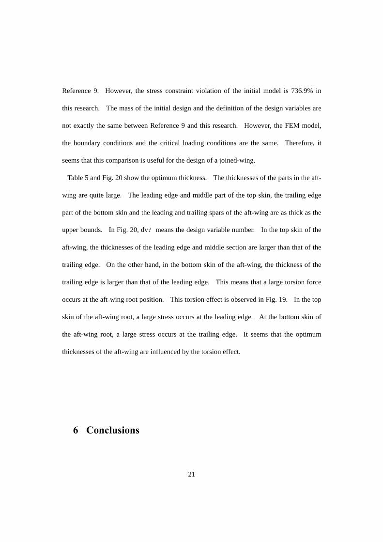
Fig. 2 Generation of equivalent static loads for displacement constraints
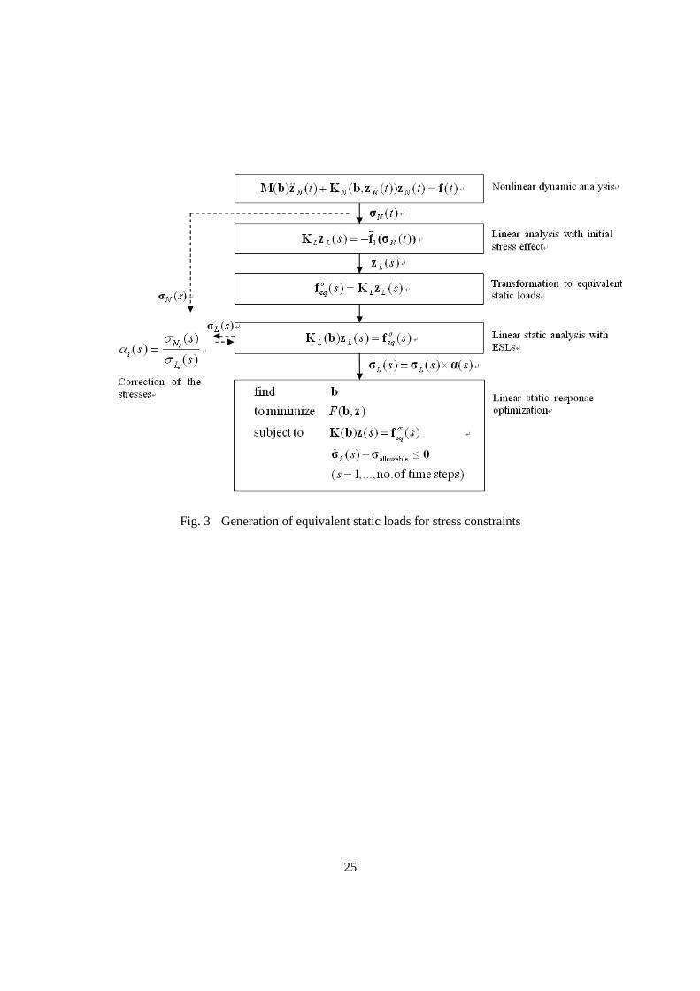
Fig. 3 Generation of equivalent static loads for stress constraints
Fig. 4 Optimization process using the equivalent static loads Fig. 5 Cantilever plate structure
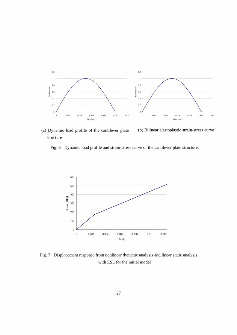
Fig. 6 Dynamic load profile and strain-stress curve of the cantilever plate structure. Fig. 7 Displacement response from nonlinear dynamic analysis and linear static analysis
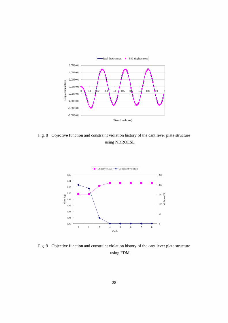
with ESL for the initial model Fig. 8 Objective function and constraint violation history of the cantilever plate structure
using NDROESL
Fig. 9 Objective function and constraint violation history of the cantilever plate structure using FDM
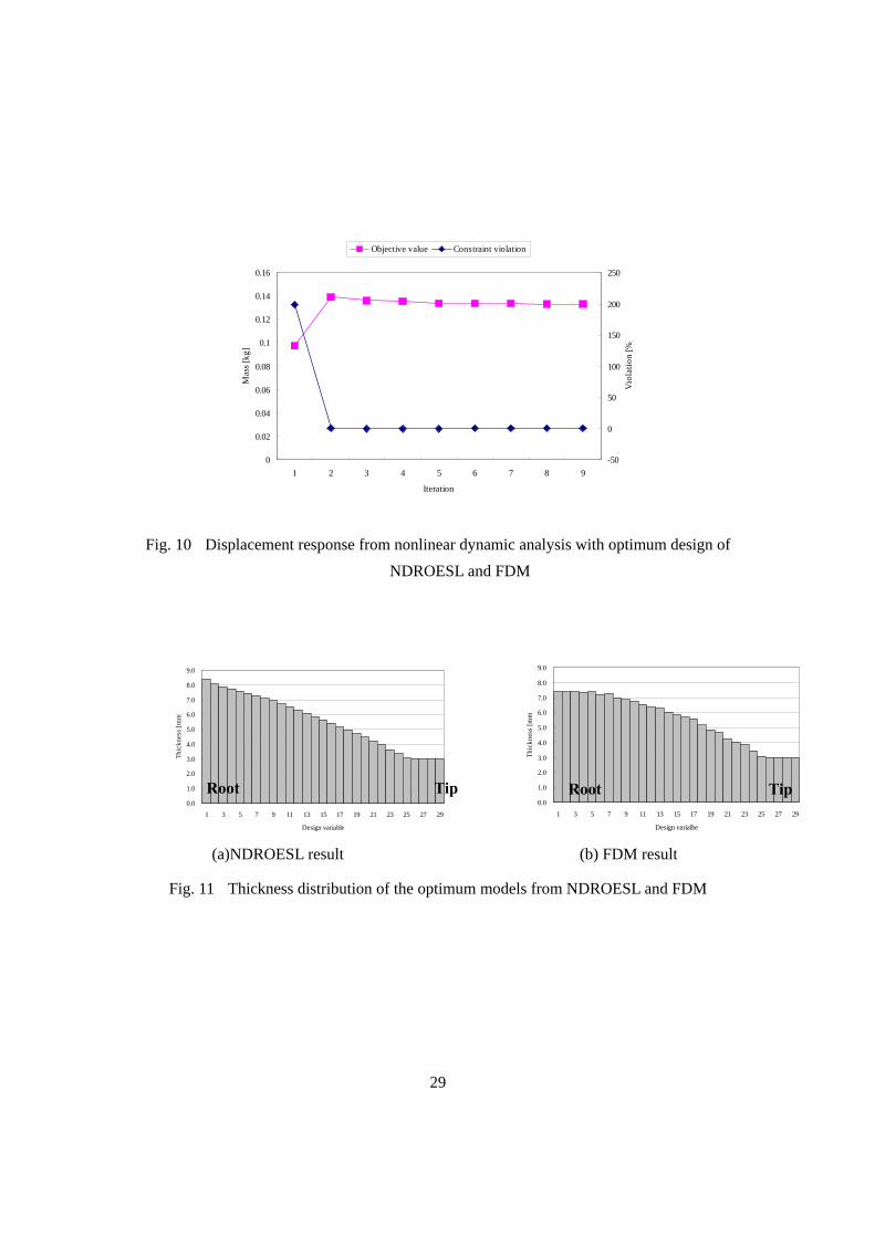
Fig. 10 Displacement response from nonlinear dynamic analysis with optimum design of NDROESL and FDM
Fig. 11 Thickness distribution of the optimum models from NDROESL and FDM
Fig. 12 Finite element modeling of the joined-wing
Fig. 13 Boundary conditions of the joined-wing
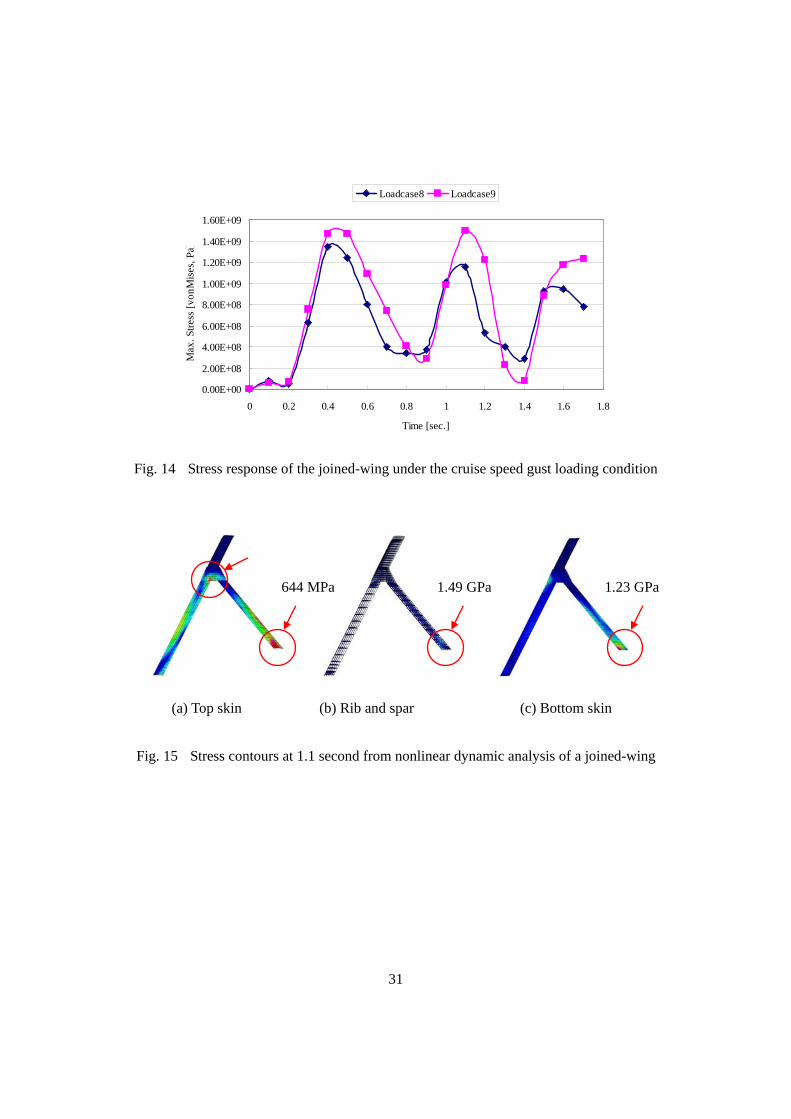
Fig. 14 Stress response of the joined-wing under the cruise speed gust loading condition
Fig. 15 Stress contours at 1.1 second from nonlinear dynamic analysis of a joined-wing
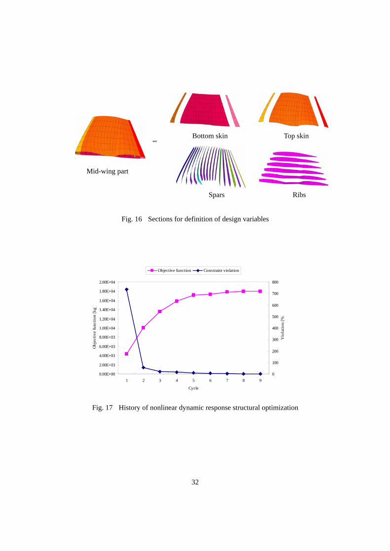
Fig. 16 Sections for definition of design variables
Fig. 17 History of nonlinear dynamic response structural optimization
Fig. 18 Stress response of the optimum design under the cruise speed gust loading condition
Fig. 19 Stress contours of the optimum design at 1.4 second
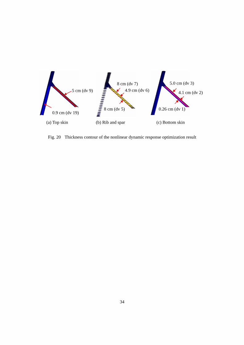
Fig. 20 Thickness contour of the nonlinear dynamic response optimization result

iii
LIST OF TABLES
Table 1 Optimum results for the cantilever plate problem
Table 2 Load data of the joined-wing
Table 3 Aerodynamic data for the joined-wing
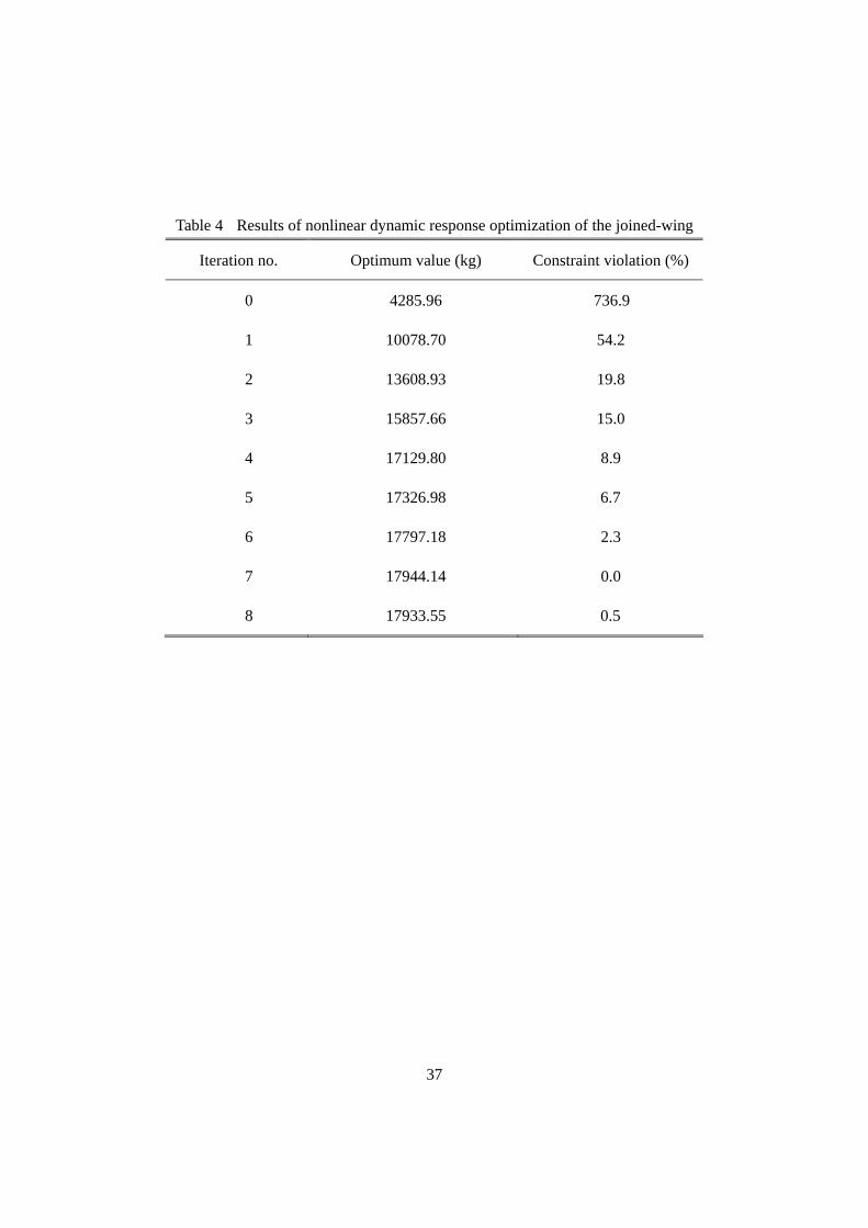
Table 4 Results of nonlinear dynamic response optimization of the joined-wing
Table 5 Optimum thicknesses from nonlinear response optimization using ESL
1
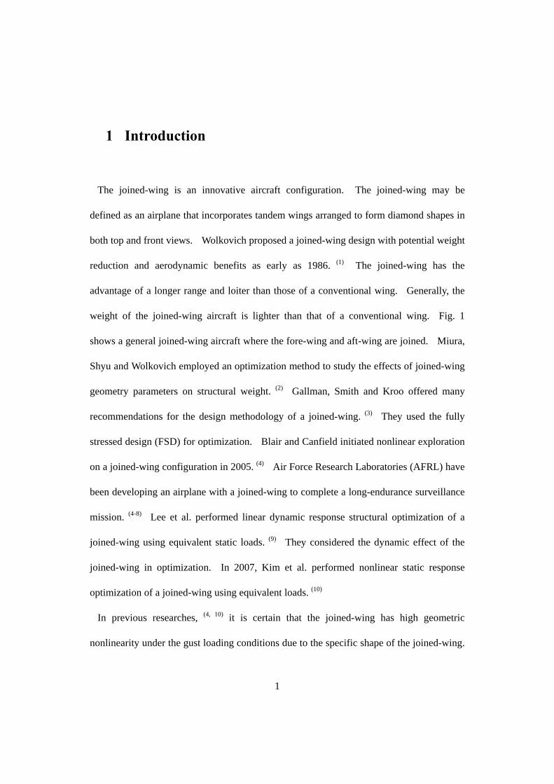
1 Introduction
The joined-wing is an innovative aircraft configuration. The joined-wing may be
defined as an airplane that incorporates tandem wings arranged to form diamond shapes in
both top and front views. Wolkovich proposed a joined-wing design with potential weight
reduction and aerodynamic benefits as early as 1986. (1) The joined-wing has the
advantage of a longer range and loiter than those of a conventional wing. Generally, the
weight of the joined-wing aircraft is lighter than that of a conventional wing. Fig. 1
shows a general joined-wing aircraft where the fore-wing and aft-wing are joined. Miura,
Shyu and Wolkovich employed an optimization method to study the effects of joined-wing
geometry parameters on structural weight. (2) Gallman, Smith and Kroo offered many
recommendations for the design methodology of a joined-wing. (3) They used the fully
stressed design (FSD) for optimization. Blair and Canfield initiated nonlinear exploration
on a joined-wing configuration in 2005. (4) Air Force Research Laboratories (AFRL) have
been developing an airplane with a joined-wing to complete a long-endurance surveillance
mission. (4-8) Lee et al. performed linear dynamic response structural optimization of a
joined-wing using equivalent static loads. (9) They considered the dynamic effect of the
joined-wing in optimization. In 2007, Kim et al. performed nonlinear static response
optimization of a joined-wing using equivalent loads. (10)
In previous researches, (4, 10) it is certain that the joined-wing has high geometric
nonlinearity under the gust loading conditions due to the specific shape of the joined-wing.
2
And structural optimization of the joined-wing has been performed from the viewpoint of
nonlinear static response. However, real forces act dynamically. Especially, the gust
loads are the most important loading conditions when an airplane wing is designed. The
gust is the movement of the air in turbulence and the gust load has a large impact on the
airplane. (11-12) The gust loads generate various dynamic effects on the aircraft wing.
Therefore, the nonlinear dynamic effect of the joined-wing should be considered in the
optimization process. However, it is very difficult to optimize a joined-wing considering
the nonlinear dynamic effect. The reason is because the conventional optimization
method is not efficient for nonlinear dynamic response structural optimization.
The calculation of the sensitivity from nonlinear dynamic analysis is fairly difficult.
This is due to the great number of nonlinear dynamic analyses required for the calculation
of the sensitivity. Therefore, the conventional gradient based optimization method is not
useful for nonlinear dynamic response optimization. (13-15) The non-gradient based
optimization method such as the response surface method can be used for nonlinear
dynamic response optimization. However, the method has several disadvantages such as
the limit of the number of design variables and inaccuracy of the solution. (16) In this
research, the equivalent static loads (ESL) method is introduced for nonlinear dynamic
response optimization. Until now, the equivalent static loads method has been used for
linear dynamic response optimization and nonlinear static response optimization. (16-21)
The concept of ESL is expanded to nonlinear dynamic response optimization.
Equivalent static loads are defined as the linear static load sets which generate the same

3
response field in linear static analysis as that from nonlinear dynamic analysis. Therefore,
if equivalent static loads are used as applied loads, the same responses from nonlinear
dynamic analysis can be considered throughout linear static response optimization. It is
well known that nonlinear dynamic analysis is quite expensive. On the other hand, linear
static analysis is not costly and the linear static response optimization theory is well
established. Equivalent static loads are made to reduce the number of nonlinear dynamic
analyses. Moreover, because the method is gradient based optimization, the solution is
exact. A detailed explanation will be introduced in Section 2.
As a small example, a cantilever plate is optimized under equivalent static loads
transformed from a dynamic load. The results are compared with those of a conventional
method where the finite difference method is employed for sensitivity calculation. A
joined-wing is optimized under dynamic gust loads. The gust loads are considered as
external loads in nonlinear dynamic response optimization. The gust loads for a joined-
wing have been calculated by the researchers of the AFRL. (4) Static loads for the gust can
be generated from an aeroelastic model which uses the Panel method. (11-12) It is difficult
to identify the exact dynamic gust load profile. Therefore, the static gust loads from
AFRL are transformed to dynamic loads using the 1-cosine function. (11) ABAQUS 6.7 (24)
is employed for nonlinear dynamic analysis and GENESIS 9.0 (25) is used for linear static
optimization.

4
2 Nonlinear dynamic structural optimization using
equivalent static loads (NDROESL)
As mentioned earlier, nonlinear dynamic response structural optimization is quite
difficult even with the modern computer system. Nonlinear analysis considering time is a
lot more expensive than nonlinear static analysis. This disadvantage is fatal for structural
optimization using the gradient based optimization method because the calculation of
sensitivity needs a large number of nonlinear dynamic analyses. On the other hand, the
approximation methods such as the response surface method (RSM) are easy to use;
however, they have a limit on the number of design variables and the solutions are not
exact. (16) The equivalent static loads method is a new and efficient method that
overcomes those weaknesses. In this section, the concept and the calculation of the
NDROESL method are explained.
2.1 Problem formulation of nonlinear dynamic response structural
optimization
The formulation for the nonlinear dynamic response optimization can be expressed as
follows:
Find mR∈b (1a)
to minimize )(bf (1b)

5
subject to 0)()())(,( =−+ tttt NNNN fzzbK)(zM(b) && (1c)
nt ,...,1=
ljtg Nj ,,1,0))(,( L=≤zb (1d)
mibbb iUiiL ,,1, L=≤≤ (1e)
M is the mass matrix which is the function of the design variable vector b . K is the
stiffness matrix which is the function of the design variable vector b and the nodal
displacement vector z , and z&& is the acceleration vector. The subscript N means that
the response is obtained from nonlinear analysis. Eq. (1c) is the governing equation of
nonlinear dynamic analysis using the finite element method. (22, 23) The constant n is the
total number of the time steps. The constant l and m are the total number of the
constraints and design variables, respectively. )(tf is the external load vector at the t th
time step. iLb and iUb are the lower bound and upper bound of the i th design variable,
respectively.
As mentioned earlier, dynamic response optimization has many time dependent
constraints. As shown in Eq. (1d), the total number of time dependent constraints is ln× .
Moreover, the calculation of the sensitivity considering the incremental step is extremely
difficult. Therefore, it is rare to perform nonlinear dynamic response structural
optimization for large scale problems.
2.2 Calculation of the equivalent static loads
The equivalent static loads (ESL) are defined as the static loads which generate the same
6
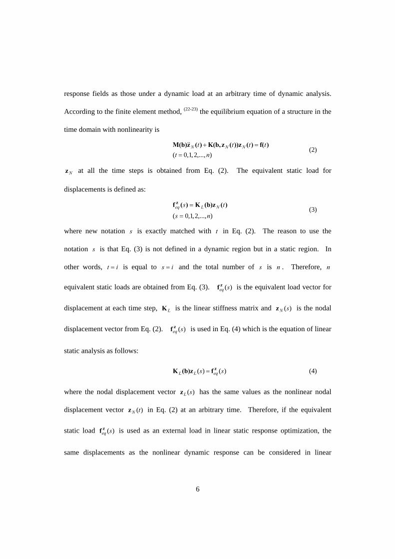
response fields as those under a dynamic load at an arbitrary time of dynamic analysis.
According to the finite element method, (22-23) the equilibrium equation of a structure in the
time domain with nonlinearity is
),...,2,1,0( nt
tttt NΝN
==+ )f()())z(zK(b,)(zM(b) &&
(2)
Nz at all the time steps is obtained from Eq. (2). The equivalent static load for
displacements is defined as:
),...,2,1,0( ns
ts NLeq
=
= )((b)zK)(f z
(3)
where new notation s is exactly matched with t in Eq. (2). The reason to use the
notation s is that Eq. (3) is not defined in a dynamic region but in a static region. In
other words, it = is equal to is = and the total number of s is n . Therefore, n
equivalent static loads are obtained from Eq. (3). )(seqzf is the equivalent load vector for
displacement at each time step, LK is the linear stiffness matrix and )(sNz is the nodal
displacement vector from Eq. (2). )(seqzf is used in Eq. (4) which is the equation of linear
static analysis as follows:
)()( ss eqLLzf(b)zK = (4)
where the nodal displacement vector )(sLz has the same values as the nonlinear nodal
displacement vector )(tNz in Eq. (2) at an arbitrary time. Therefore, if the equivalent
static load )(seqzf is used as an external load in linear static response optimization, the
same displacements as the nonlinear dynamic response can be considered in linear

7
response optimization. The equivalent static loads are used as multiple loading conditions
for linear static response optimization and Fig. 2 presents this process.
Although the load )(seqzf can generate the same displacements as the nonlinear
displacements at all the time steps, it does not generate the same stress responses because
the relationships between the strain and displacement as well as the strain and stress have
nonlinearity. Thus, the equivalent static loads for the stresses are separately calculated.
The stress response )(tNσ is obtained from Eq. (2) of nonlinear dynamic analysis. The
obtained stresses are used as initial stresses of linear static analysis. The equivalent static
loads for stresses are calculated as follows:
))(()( ts NILL σf(b)zK σ −= (5)
)()( ss LLeqσσ (b)zKf = (6)
where )(seqσf is the equivalent static load vector for the stress response, LK is the linear
stiffness matrix, )(tNσ from Eq. (2) is utilized as the initial stress effect ))(( tNI σf− in Eq.
(5) for linear static analysis. )(sLσz is the displacement vector from Eq. (5) and )(seq
σf is
calculated by multiplying LK and )(sLσz as shown in Eq. (6).
)(seqσf is used as follows:
)()( ss eqLLσf(b)zK = (7)
The stress response )(sLσ is obtained from Eq. (7) of linear analysis. However, this
stress response may not be exactly the same as that from nonlinear analysis because the
8
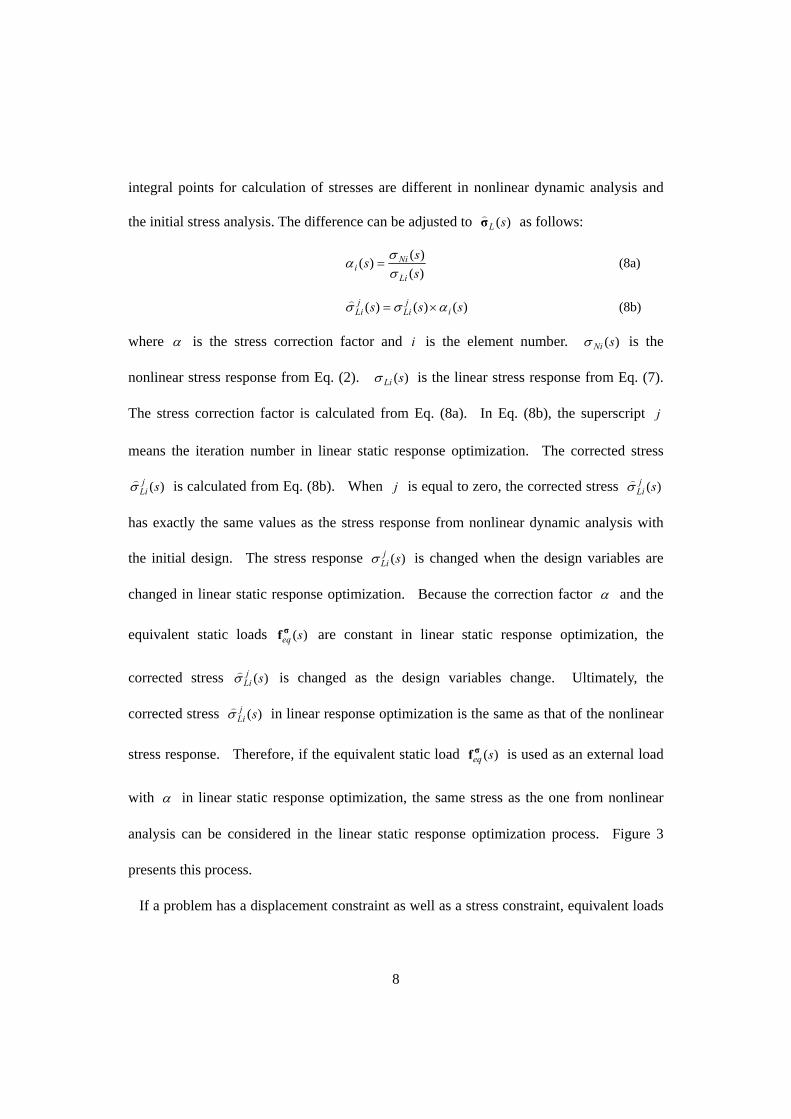
integral points for calculation of stresses are different in nonlinear dynamic analysis and
the initial stress analysis. The difference can be adjusted to )(sLσ) as follows:
)()()(
sss
Li
Nii σ
σα = (8a)
)()()( sss ij
Lij
Li ασσ ×=) (8b)
where α is the stress correction factor and i is the element number. )(sNiσ is the
nonlinear stress response from Eq. (2). )(sLiσ is the linear stress response from Eq. (7).
The stress correction factor is calculated from Eq. (8a). In Eq. (8b), the superscript j
means the iteration number in linear static response optimization. The corrected stress
)(sjLiσ) is calculated from Eq. (8b). When j is equal to zero, the corrected stress )(sj
Liσ)
has exactly the same values as the stress response from nonlinear dynamic analysis with
the initial design. The stress response )(sjLiσ is changed when the design variables are
changed in linear static response optimization. Because the correction factor α and the
equivalent static loads )(seqσf are constant in linear static response optimization, the
corrected stress )(sjLiσ) is changed as the design variables change. Ultimately, the
corrected stress )(sjLiσ) in linear response optimization is the same as that of the nonlinear
stress response. Therefore, if the equivalent static load )(seqσf is used as an external load
with α in linear static response optimization, the same stress as the one from nonlinear
analysis can be considered in the linear static response optimization process. Figure 3
presents this process.
If a problem has a displacement constraint as well as a stress constraint, equivalent loads

9
should be calculated with respect to each response, and the sets of the equivalent static
loads are utilized in linear static response optimization as multiple loading conditions.
2.3 The steps for nonlinear dynamic response structural optimization
using equivalent static loads (NDROESL)
The overall process of the NDROESL algorithm is illustrated in Fig. 4. The steps of the
algorithm are as follows:
Step 1. Set initial design variables and parameters (design variables: )0()( bb =k , cycle
number: 0=k , convergence parameter: a small number ε ).
Step 2. Perform nonlinear dynamic analysis with )(kb . Hence the linear stiffness matrix
and nonlinear responses are obtained.
Step 3. When k = 0, go to Step 4. When k > 0, if
ε≤− − )1()( kk bb (9a)
),,1;,,1(
0))(),(,( )1(
ntlj
ttg NNk
j
LL ==
≤+ σzb (9b)
then terminate the process. Otherwise, go to Step 4. If Eq (9a) is satisfied and
Eq (9b) is not satisfied, reduce the convergence parameter ε to have a smaller
value and go to Step 4.
Step 4. Calculate the equivalent static load sets as follows:
)()()(, ts NLk
eq (b)zKf z = and )()()(, ts LLk
eqσσ (b)zKf = (10)
Step 5. Solve the following linear static response optimization problem:

10
Find )1( +kb (11a)
to minimize )( )1( +kf b (11b)
subject to 0)()()( )(,)1( =−+ ss keq
kL
zfzbK (11c)
0)()()( )(,)1( =−+ ss keq
kL
σfzbK (11d)
ns ,...,1=
ljssg kj ,,1,0))(),(,( )1( L
) =≤+ σzb (11e)
mikiU
ki
kiL ,,1,)1()1()1( L=≤≤ +++ bbb (11f)
The external load )(seqf is the equivalent static load vector and n2 equivalent
static load sets are used as multiple loading conditions during the linear static
response optimization process.
Step 6. Update the design results, set 1+= kk and go to Step 2.
2.4 A small scale example: nonlinear dynamic structural optimization
of a cantilever plate
A small scale problem is solved by using the NDROESL method to validate the method.
The model is a cantilever plate with 120 shell elements. The loading and boundary
conditions are illustrated in Fig. 5. Figure 6(a) presents the dynamic load profile. The
duration time is 0.01 second and the total analysis time is 0.1 second. ABAQUS 6.7 (24) is
used for the nonlinear dynamic analysis. The implicit method is used with a constant
incremental size of 0.0002. The total number of time steps is five hundred and the total

11
number of equivalent static loads is the same. Figure 6(b) shows the strain-stress curve of
the used material for this problem. The material has bilinear elastoplastic strain-stress
curve. The Young’s modulus is 68.9 GPa and the tangent modulus is 34.5 GPa. The
yield strength is 172 MPa. The Poisson ratio is 0.35 and the density is 2710 kg/m3. Both
geometric and material nonlinearities are considered in this problem.
Figure 7 illustrates the maximum displacement responses from nonlinear dynamic
analysis and linear static analysis with ESL for the initial model. As shown, the responses
are exactly the same. The maximum difference is 4x10⁻⁸ m. Therefore, the
transformation is validated. The optimization formulation is as follows:
Find )29,,1( L=ibi (12a)
to minimize Mass (12b)
subject to )500,,1(mm0.20tip L=≤ ppδ (12b)
mm0.10mm0.3 ≤≤ ib (12c)
The design variables are the thicknesses. The cantilever plate is divided into twenty
nine sections with respect to the x direction and the total number of design variables is
twenty nine. The objective function is the mass. The constraint is that the magnitude of
maximum displacement should be less than the allowable displacement of 20 mm at all the
time steps.
This problem is solved by NDROESL as well as by a conventional method. The
modified method of feasible directions algorithm in a commercial optimization code DOT
5.7 is used for the conventional method. (26) The finite difference method (FDM) is

12
employed for sensitivity analysis. The results of both methods are compared.
Figures 8 and 9 illustrate the history of the objective function and constraint violation for
NDROESL and FDM, respectively. Table 1 shows the optimization results for the
cantilever plate problem. As shown in the table, the optimum mass is almost the same.
The displacement constraint is active at the optima of both methods. Figure 10 presents
the maximum displacements from nonlinear dynamic analyses at the optima of both
methods. They are almost the same. Since the solution from the conventional method
can be considered as a mathematical optimum, the quality of the solution from NDROESL
is excellent.
The efficiency of the two methods is quite different. Only eight nonlinear dynamic
analyses are required in NDROESL while three hundred and sixty five analyses are
required in the conventional method using FDM. The same computer, Intel Pentium Dual
CPU 3.20 GHz, 3.25 GB RAM, (27) is used for the analysis and optimization. In total
CPU time, NDROESL requires 22 minutes while FDM requires 486 minutes. Figure 11
illustrates the thickness distribution of the optimum models from both methods. The
thickness of the root is thick and that of the tip is thin in both methods; however, the
profiles are different. The difference of sensitivity causes the difference of the optimum
profile. The linear response is used for the calculation of sensitivity in NDROESL. On
the other hand, the nonlinear response is directly used for the calculation of sensitivity in
the conventional method using FDM. The difference of sensitivity is reduced as the cycle
is repeated. The results of NDROESL are almost the same as those of the conventional
13
method using FDM. However, NDROESL is more efficient than the conventional method.
Conceptually, it seems that the joined-wing structure is a cantilever type structure. The
root of the wing is fixed at the fuselage. Several thousand shell elements are used for the
finite element method of the structure. From the next section, the analysis and
optimization of the joined-wing structure will be explained. Since it is a very large scale
problem, the conventional method is almost impossible to use. Therefore, only the
NDROESL method is used for nonlinear dynamic structural optimization of the joined-
wing.
3 Analysis of the joined-wing
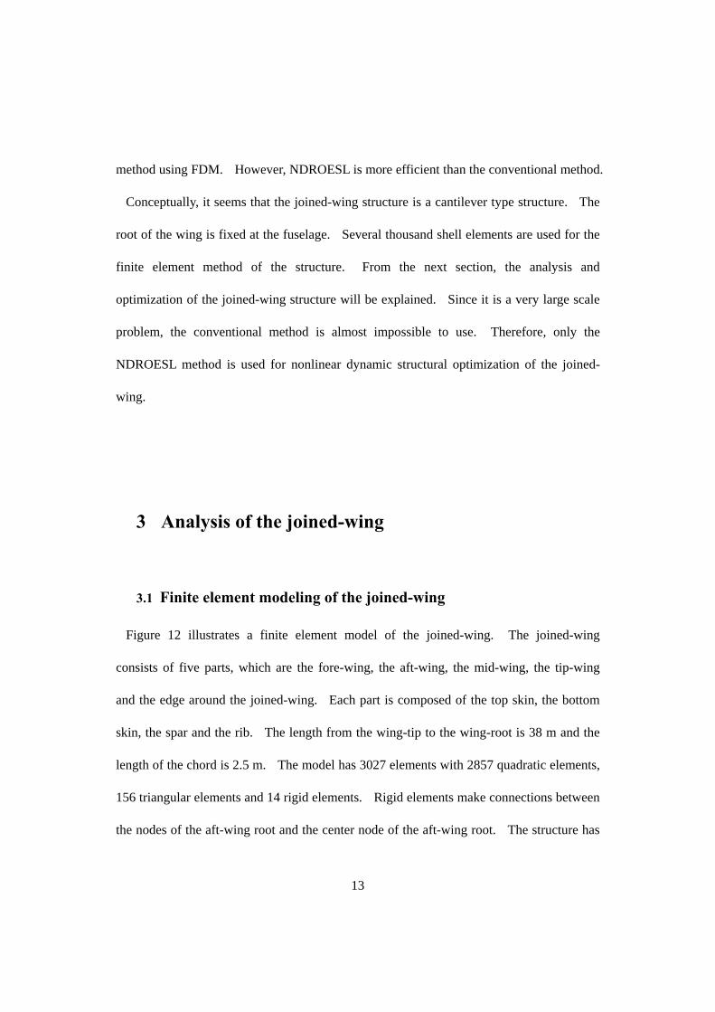
3.1 Finite element modeling of the joined-wing
Figure 12 illustrates a finite element model of the joined-wing. The joined-wing
consists of five parts, which are the fore-wing, the aft-wing, the mid-wing, the tip-wing
and the edge around the joined-wing. Each part is composed of the top skin, the bottom
skin, the spar and the rib. The length from the wing-tip to the wing-root is 38 m and the
length of the chord is 2.5 m. The model has 3027 elements with 2857 quadratic elements,
156 triangular elements and 14 rigid elements. Rigid elements make connections between
the nodes of the aft-wing root and the center node of the aft-wing root. The structure has

14
two kinds of aluminum materials. One has the Young’s modulus of 72.4 GPa, the shear
modulus of 27.6 GPa and the density of 2770 kg/m3. The other has 36.2 GPa, 13.8 GPa
and 2770 kg/m3, respectively. The former material is used for the entire elements except
for the edge part. The latter material is only used for the elements of the edge part.
3.2 Loading conditions of the joined-wing
Eleven static loading conditions for structural optimization have been defined by the
AFRL. (4) These loading conditions are composed of seven maneuver loads, two gust
loads, one take-off load and one landing load as shown in Table 2. Each loading
condition has a different loading direction and magnitude. The gust loading conditions
are especially important in these loading conditions. Gust is the movement of the air in
turbulence and the gust load has a large impact on the airplane. Static loads for the gust
can be generated from an aeroelastic model which uses the Panel method. (12) The Panel
method is used to calculate the velocity distribution along the surface of the airfoil. Panel
methods have been developed to analyze the flow field around arbitrary bodies in two and
three dimensions. The surface of the airfoil is divided into trapezoid panels.
Mathematically, each panel generates the velocity on it. This velocity can be expressed
by relatively simple equations which contain geometric relations, such as distances and
angles between the panels. The Panel method is referred to as the boundary element
method in some publications. (12) Detailed explanation of the Panel method is out of
scope of this work.

15
The real gust load acts dynamically on the airplane. Also, dynamic loads are required
for optimization with equivalent static loads. However, the generation of exact dynamic
loads which consider the nonlinear dynamic behavior of the airplane is very difficult.
Therefore, the static gust loads of Reference 4 are transformed to dynamic loads.
Generally, there are several methods for generating dynamic gust loads. (11) Here, the
approximated dynamic load is evaluated by multiplying the static load by the 1-cosine
function.
The duration time of the dynamic gust load is calculated from the following equation. (11)
⎟⎠⎞
⎜⎝⎛ −=
CsUU de
252cos1
2π (13)
where U is the velocity of the gust load, deU is the maximum velocity of the gust load, s
is the distance penetrated into the gust and C is the geometric mean chord of the wing.
The conditions for the coefficients are shown in Table 3. From Table 3 and Eq. (13), the
duration time is 0.374 seconds. The airplane stays in the gust for 0.374 seconds.
The dynamic gust load is calculated as follows:
⎟⎠⎞
⎜⎝⎛ −×= tFF
374.02cos1staticdynamicπ (14)
where staticF is the static gust load which is the eighth or ninth load in Table 2. It is noted
that the period of the gust load is 0.374 second and the duration time of the dynamic load is
0.374 second. The dynamic load becomes zero after 0.374 second.
3.3 Boundary conditions of the joined-wing
The roots of the fore-wing and the aft-wing are joined to the fuselage. That is, the entire

16
part of the fore-wing root is attached to the fuselage. Therefore, all the degrees of
freedom in six directions are fixed. On the other hand, the aft-wing root can be rotated
with respect to the y-axis in Fig. 13. The boundary nodes of the aft-wing root are rigidly
connected to the center node. The center node has an enforced rotation with respect to the
y-axis. The boundary nodes are set free in the x and z translational directions. Other
degrees of freedom are fixed. The enforced rotation generates torsion on the aft-wing and
has quite an important aerodynamic effect. The amounts of the enforced rotation are from
-0.0897 radian to 0.0 radian. These rotational values are different in each mission leg.
The boundary conditions are illustrated in Fig. 13.
3.4 Nonlinear dynamic analysis of the joined-wing
Nonlinear dynamic analysis is performed under the gust loading conditions. Geometric
nonlinearity is considered in nonlinear dynamic analysis. The dynamic loads are
generated by Eq. (14). ABAQUS 6.7 (24) is used for nonlinear dynamic analysis. HP-UX
Itanium II computer is used for nonlinear dynamic analysis (28) As mentioned before, the
duration time of the dynamic gust load is 0.374 second and the total analysis time is 1.8
seconds. The size of the time step is 0.1 second. Then, the stress response is recorded
every 0.1 second. Therefore, each loading condition has 18 time steps. Then, the total
number of time steps is thirty six for the two gust loading conditions. In the linear static
response optimization process using the equivalent static loads, thirty six static loading
conditions are utilized as multiple loading conditions.

17
Figure 14 illustrates the von Mises stresses from nonlinear dynamic analysis. The stress
fluctuates and the maximum stress occurs after 0.374 second which is the duration time of
the dynamic load. Moreover, the maximum stress occurs within 1.8 seconds. Generally,
the maximum stress occurs at the wing root. Figure 15 presents the stress contour of the
joined-wing at 1.1 second and the maximum stress occurs under the gust loading condition
9.
4 Structural optimization of the joined-wing
4.1 Definition of design variables
As mentioned earlier, the FEM model of the joined-wing has 3027 finite elements. It is
not reasonable to select the properties of all the elements as design variables for
optimization. Thus, the design variable linking technology is utilized. The wing
structure is divided into forty eight sections and each section has the same thickness. The
finite element model is adopted from Reference 4. The joined-wing is divided into five
parts as illustrated in Fig. 12. Each part is composed of the top skin, the bottom skin, the
spar and the rib. Fig. 16 presents the division of the mid-wing. The top and bottom
skins are divided into three sections. The sections are the wing-skin-front, the wing-skin-
middle and the wing-skin-rear. The spars of the mid-wing are divided into seven sections.
18
The spars of other wings are divided into three sections. Other parts such as the fore-wing,
the aft-wing, the wing tip and the edge are divided in the same manner. The wing tip and
the edge parts are not used as design variables. Therefore, only thirty four sections among
the forty eight sections are used as design variables. Design variables are defined based
on Reference 9.
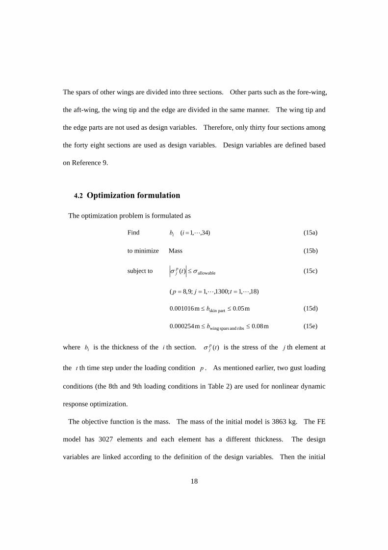
4.2 Optimization formulation
The optimization problem is formulated as
Find )34,,1( L=ibi (15a)
to minimize Mass (15b)
subject to allowable)( σσ ≤tpj (15c)
)18,,1;1300,,1;9,8( LL === tjp
m05.0m001016.0 partskin ≤≤ b (15d)
m08.0m000254.0 ribsandsparswing ≤≤ b (15e)
where ib is the thickness of the i th section. )(tpjσ is the stress of the j th element at
the t th time step under the loading condition p . As mentioned earlier, two gust loading
conditions (the 8th and 9th loading conditions in Table 2) are used for nonlinear dynamic
response optimization.
The objective function is the mass. The mass of the initial model is 3863 kg. The FE
model has 3027 elements and each element has a different thickness. The design
variables are linked according to the definition of the design variables. Then the initial

19
mass is 4285 kg. The upper and lower bounds are defined for each part. 0.001016 m
and 0.000254 m are used as the lower bounds of the skin part and wing spars, and that of
rib parts, respectively. 0.05 m is used as the upper bound of the skin part and 0.08 m is
used as the upper bounds of the spars and rib parts.
The material of the joined-wing is aluminum. (4) The allowable von Mises stress for
aluminum is set by 269MPa. Since the safety factor 1.5 is used, the allowable stress is
reduced to 179 MPa. Stresses of all the elements except for the edge part and the wing tip
part should be less than the allowable stress 179 MPa.
5 Discussion
5.1 The results of nonlinear dynamic response optimization
Nonlinear dynamic response structural optimization of the joined-wing is carried out
using equivalent static loads. Two gust loading conditions are used as external dynamic
loads. Each loading condition is divided into eighteen time steps from 0.0 second to 1.8
second. According to the equivalent static loads concept, thirty six static loading
conditions are defined for the two gust loads.
Table 4 and Fig. 17 show the history of the optimization process. The objective
function is increased by 318.4 percent from 4285.96 kg to 17933.55 kg. It is noted that
the constraints are satisfied when nonlinear dynamic analysis is performed with the
20
optimum solution. The stress response of the optimum is illustrated in Fig. 18. The
critical stresses occur at 0.2 second, 0.4 second, 0.9 second and 1.4 second. Figure 19
illustrates the stress contours of the optimum at 1.4 second. The maximum stress of
optimum occurs at element 1407 which is located in the top skin of the aft-wing root. The
magnitude of the maximum stress is 179.9 MPa at the time of 1.4 second. Generally, the
effect of loading condition 9 (cruise speed gust load) is more severe than that of loading
condition 8 (maneuver speed gust).
The violation of the stress constraint of cycle 7 is smaller than that of cycle 8. However,
the mass of cycle 8 is smaller than that of cycle 7. The process is considered as
converged when the difference between the design variables of the current cycle and those
of the previous cycle is smaller than a given small number. The convergence criteria are
satisfied in cycle 8. Both results of cycle 7 and 8 may be selected as the optimum design.
5.2 Discussion about the optimum design
As mentioned earlier, the mass is increased by 318.4 percent from 4285.96 kg to
17933.55 kg. Overall, the optimum thickness from nonlinear dynamic response structural
optimization is larger than that of the initial model. In Reference 9, where linear dynamic
response optimization of a joined-wing is performed, the optimum mass is 12725.52 kg.
The optimum mass of nonlinear dynamic response optimization is larger than that of linear
dynamic response optimization. It is reasonable because the geometric nonlinearity is
added in this research. The stress constraint violation of the initial model is 344.21% in
21
Reference 9. However, the stress constraint violation of the initial model is 736.9% in
this research. The mass of the initial design and the definition of the design variables are
not exactly the same between Reference 9 and this research. However, the FEM model,
the boundary conditions and the critical loading conditions are the same. Therefore, it
seems that this comparison is useful for the design of a joined-wing.
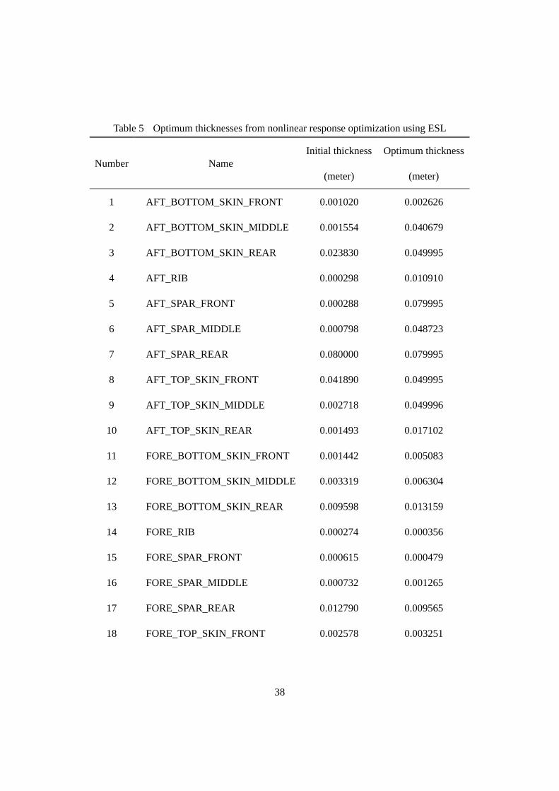
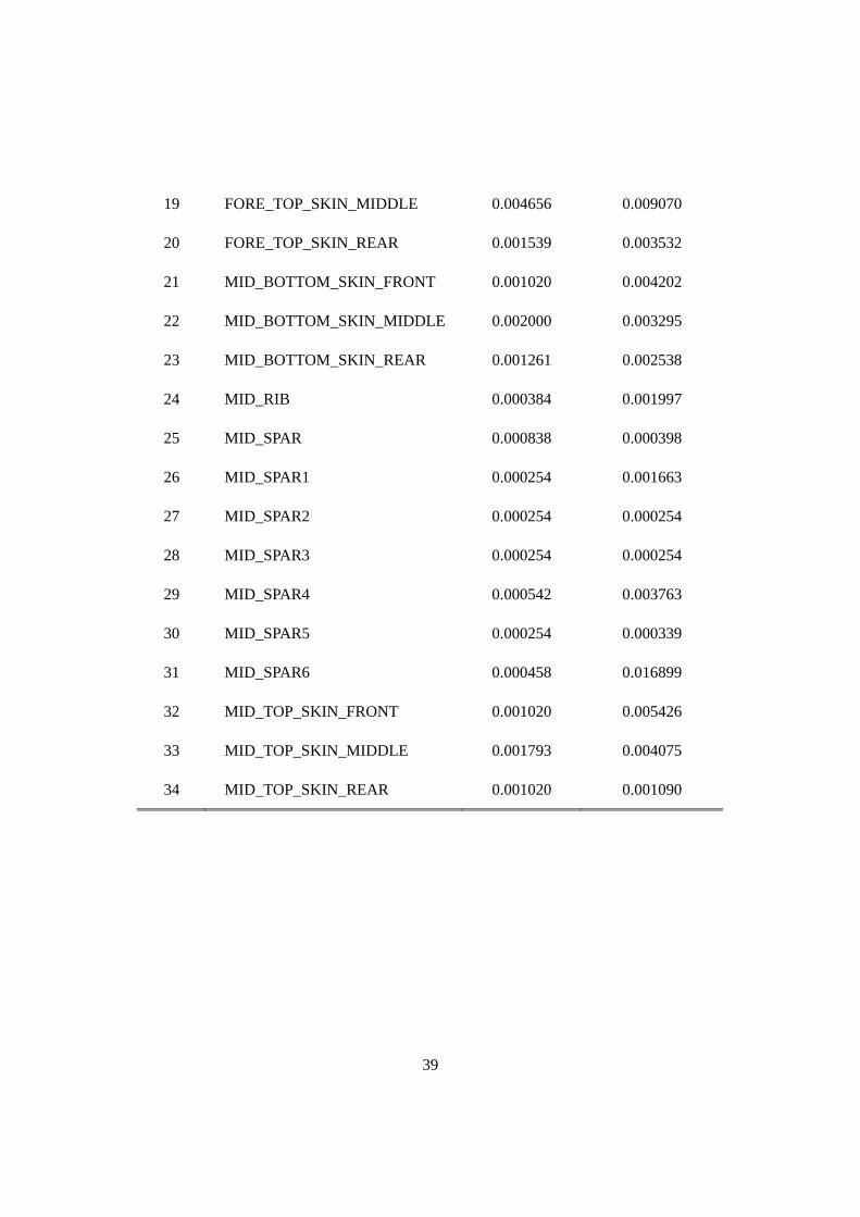
Table 5 and Fig. 20 show the optimum thickness. The thicknesses of the parts in the aft-
wing are quite large. The leading edge and middle part of the top skin, the trailing edge
part of the bottom skin and the leading and trailing spars of the aft-wing are as thick as the
upper bounds. In Fig. 20, dv i means the design variable number. In the top skin of the
aft-wing, the thicknesses of the leading edge and middle section are larger than that of the
trailing edge. On the other hand, in the bottom skin of the aft-wing, the thickness of the
trailing edge is larger than that of the leading edge. This means that a large torsion force
occurs at the aft-wing root position. This torsion effect is observed in Fig. 19. In the top
skin of the aft-wing root, a large stress occurs at the leading edge. At the bottom skin of
the aft-wing root, a large stress occurs at the trailing edge. It seems that the optimum
thicknesses of the aft-wing are influenced by the torsion effect.
6 Conclusions

22
The joined-wing is defined as an airplane that incorporates tandem wings arranged to
form diamond shapes in both top and front views. The joined-wing configuration has
many advantages from the viewpoint of aerodynamic performance and weight reduction.
However, due to the specific shape of the joined-wing, it has large geometric nonlinearity
under the gust loading conditions. The real gust acts dynamically. Therefore, the
nonlinear dynamic behavior should be considered in structural optimization of a joined-
wing. The dynamic gust load profile is calculated by multiplying the static gust loads by
the 1-cosine function.
The equivalent static loads are used for nonlinear dynamic response structural
optimization of a joined-wing. The existing concepts of the equivalent static loads are
expanded for nonlinear dynamic response optimization. This is called nonlinear dynamic
response optimization using equivalent static loads. (NDROESL) The equivalent static
loads are defined as the linear static load sets which generate the same response field in
linear static analysis as that from nonlinear dynamic analysis. Therefore, if equivalent
static loads are used as applied loads, the same responses from nonlinear dynamic analysis
can be considered in linear static response optimization. Equivalent static loads are made
to reduce the number of nonlinear dynamic analyses. Also, because the method is
gradient based optimization, the solution is exact. An example of the cantilever plate is
solved by NDROESL as well as the conventional method using the finite difference
method. By comparing results, NDROESL is more efficient than the conventional
method. And the objective function values of the two methods are almost the same.
23
The optimum design considering the nonlinear dynamic effect of the joined-wing
satisfies all the stress constraints. The joined-wing is divided into forty eight sections and
the thicknesses of thirty four sections are used as design variables for nonlinear dynamic
response optimization. The mass is increased by 318.4 percent. It is because the
constraint violation of the initial model is quite large and the thicknesses of almost all the
sections are increased. It is noted that the optimum thicknesses of the leading edge of the
top skin and those of the trailing edge of the bottom skin in the aft-wing are 5 cm, which is
the upper bound. Only eight nonlinear dynamic analyses are required for nonlinear
dynamic response structural optimization of the joined-wing. Nonlinear dynamic
response optimization of a joined-wing using the proposed method is very successful and
efficient although the problem is fairly large scale.
24
Fig. 1 Configuration of the joined-wing
Fig. 2 Generation of equivalent static loads for displacement constraints
)()()()()( tttt NNNN f)zz(b,KzbM =+&&
)()( ts NLz
eq zKf =
)stepstimeofno.,...,1()(
)()()(tosubject)(minimizeto
find
allowable
=≤−
=
ss
ssF
L
zeq
0zz
fzbKzb,
b
)(tNz
Nonlinear dynamic analysis
Transformation to equivalent static loads
Linear static analysis with ESLs
Linear static response optimization
)()( ss zeqLL f(b)zK =
25
Fig. 3 Generation of equivalent static loads for stress constraints

26
Fig. 4 Optimization process using the equivalent static loads
Fig. 5 Cantilever plate structure
x y
x z
60 N
0.03 m
0.3 m
Start
Perform nonlinear dynamic analysis
Calculate equivalent static loads
Satisfy termination criteria?
End
Solve linear static response optimization
Update design variables
27
Fig. 6 Dynamic load profile and strain-stress curve of the cantilever plate structure.
Fig. 7 Displacement response from nonlinear dynamic analysis and linear static analysis with ESL for the initial model
0
100
200
300
400
500
600
0 0.002 0.004 0.006 0.008 0.01 0.012
Strain
Stre
ss [M
Pa]
(a) Dynamic load profile of the cantilever plate structure
0
0.2
0.4
0.6
0.8
1
1.2
0 0.002 0.004 0.006 0.008 0.01 0.012
Time [sec.]
Scal
e fa
ctor
0
0.2
0.4
0.6
0.8
1
1.2
0 0.002 0.004 0.006 0.008 0.01 0.012
Time [sec.]
Scal
e fa
ctor
(b) Bilinear elastoplastic strain-stress curve
28
Fig. 8 Objective function and constraint violation history of the cantilever plate structure using NDROESL
Fig. 9 Objective function and constraint violation history of the cantilever plate structure using FDM
-8.00E+01
-6.00E+01
-4.00E+01
-2.00E+01
0.00E+00
2.00E+01
4.00E+01
6.00E+01
0 0.1 0.2 0.3 0.4 0.5 0.6 0.7 0.8 0.9 1
Time (Load case)
Dis
plac
emen
t [m
m
Real displacement ESL displacement
0.00
0.02
0.04
0.06
0.08
0.10
0.12
0.14
0.16
1 2 3 4 5 6 7 8
Cycle
Mas
s [kg
]
0
50
100
150
200
250
Vio
latio
n [%
]
Objective value Constraint violation
29
Fig. 10 Displacement response from nonlinear dynamic analysis with optimum design of NDROESL and FDM
Fig. 11 Thickness distribution of the optimum models from NDROESL and FDM
0.0
1.0
2.0
3.0
4.0
5.0
6.0
7.0
8.0
9.0
1 3 5 7 9 11 13 15 17 19 21 23 25 27 29
Design variable
Thic
knes
s [m
m]
0.0
1.0
2.0
3.0
4.0
5.0
6.0
7.0
8.0
9.0
1 3 5 7 9 11 13 15 17 19 21 23 25 27 29
Design varialbe
Thic
knes
s [m
m]
(a)NDROESL result (b) FDM result
Root Tip Root Tip
0
0.02
0.04
0.06
0.08
0.1
0.12
0.14
0.16
1 2 3 4 5 6 7 8 9
Iteration
Mas
s [kg
]
-50
0
50
100
150
200
250
Vio
latio
n [%
]
Objective value Constraint violation

30
Fig. 12 Finite element modeling of the joined-wing
Fig. 13 Boundary conditions of the joined-wing
Boundary nodes: all degrees of freedom
Boundary nodes: x and z translational direction - free Center node:
y-axis rotational direction
- free
x y
z
Top skin
Bottom skin
Spar Rib
Edge part Whole model
Mid-wing
Fore-wing
Aft-wing
Tip-wing
31
0.00E+00
2.00E+08
4.00E+08
6.00E+08
8.00E+08
1.00E+09
1.20E+09
1.40E+09
1.60E+09
0 0.2 0.4 0.6 0.8 1 1.2 1.4 1.6 1.8
Time [sec.]
Max
. Stre
ss [v
onM
ises
, Pa]
Loadcase8 Loadcase9
Fig. 14 Stress response of the joined-wing under the cruise speed gust loading condition
(a) Top skin (b) Rib and spar (c) Bottom skin
Fig. 15 Stress contours at 1.1 second from nonlinear dynamic analysis of a joined-wing
1.49 GPa 1.23 GPa 644 MPa
32
Fig. 16 Sections for definition of design variables
0.00E+00
2.00E+03
4.00E+03
6.00E+03
8.00E+03
1.00E+04
1.20E+04
1.40E+04
1.60E+04
1.80E+04
2.00E+04
1 2 3 4 5 6 7 8 9
Cycle
Obj
ectiv
e fu
nctio
n [k
g]
0
100
200
300
400
500
600
700
800V
iola
tion
[%]
Objective function Constraint violation
Fig. 17 History of nonlinear dynamic response structural optimization
=Bottom skin Top skin
Spars Ribs
Mid-wing part

33
0.00E+00
3.00E+07
6.00E+07
9.00E+07
1.20E+08
1.50E+08
1.80E+08
2.10E+08
0 0.2 0.4 0.6 0.8 1 1.2 1.4 1.6 1.8
Time [sec.]
Max
. Stre
ss [v
onM
ises
, Pa]
Loadcase8 Loadcase9
Fig. 18 Stress response of the optimum design under the cruise speed gust loading condition
(a) Top skin (b) Rib and spar (c) Bottom skin
Fig. 19 Stress contours of the optimum design at 1.4 second
179 9 MPa123 MPa
179 MPa
34
(a) Top skin (b) Rib and spar (c) Bottom skin
Fig. 20 Thickness contour of the nonlinear dynamic response optimization result
5 cm (dv 9)
0.9 cm (dv 19) 8 cm (dv 5)
8 cm (dv 7) 4.9 cm (dv 6)
5.0 cm (dv 3)
0.26 cm (dv 1)
4.1 cm (dv 2)

35
Table 1 Optimum results for the cantilever plate problem
Initial Optimum of
NDROESL
Optimum of
FDM
Mass 0.09756 kg 0.13353 kg 0.13314 kg
Maximum displacement 59.6 mm 20.00 mm 20.06 mm
Number of iterations (cycles) 8 9
Number of nonlinear transient
analyses 8 365
Number of nonlinear transient
analyses except for gradient call 104
Total number of iterations for linear
response optimization 24
Total CPU time 22 minutes 486 minutes

36
Table 2 Load data of the joined-wing
Number of loading condition Load type Mission leg
1 2.5 g PullUp Ingress
2 2.5 g PullUp Ingress
3 2.5 g PullUp Loiter
4 2.5 g PullUp Loiter
5 2.5 g PullUp Egress
6 2.5 g PullUp Egress
7 2.5 g PullUp Egress
8 Gust (Maneuver) Descent
9 Gust (Cruise) Descent
10 Taxi (1.75 g impact) Take-off
11 Impact (3.0 g landing) Landing
Table 3 Aerodynamic data for the joined-wing
Gust maximum velocity 18.2 m/s
Flight velocity 167 m/s
Geometric mean chord of wing 2.5 m
Distance penetrated into gust 62.5 m
37
Table 4 Results of nonlinear dynamic response optimization of the joined-wing
Iteration no. Optimum value (kg) Constraint violation (%)
0 4285.96 736.9
1 10078.70 54.2
2 13608.93 19.8
3 15857.66 15.0
4 17129.80 8.9
5 17326.98 6.7
6 17797.18 2.3
7 17944.14 0.0
8 17933.55 0.5
38
Table 5 Optimum thicknesses from nonlinear response optimization using ESL
Number Name Initial thickness
(meter)
Optimum thickness
(meter)
1 AFT_BOTTOM_SKIN_FRONT 0.001020 0.002626
2 AFT_BOTTOM_SKIN_MIDDLE 0.001554 0.040679
3 AFT_BOTTOM_SKIN_REAR 0.023830 0.049995
4 AFT_RIB 0.000298 0.010910
5 AFT_SPAR_FRONT 0.000288 0.079995
6 AFT_SPAR_MIDDLE 0.000798 0.048723
7 AFT_SPAR_REAR 0.080000 0.079995
8 AFT_TOP_SKIN_FRONT 0.041890 0.049995
9 AFT_TOP_SKIN_MIDDLE 0.002718 0.049996
10 AFT_TOP_SKIN_REAR 0.001493 0.017102
11 FORE_BOTTOM_SKIN_FRONT 0.001442 0.005083
12 FORE_BOTTOM_SKIN_MIDDLE 0.003319 0.006304
13 FORE_BOTTOM_SKIN_REAR 0.009598 0.013159
14 FORE_RIB 0.000274 0.000356
15 FORE_SPAR_FRONT 0.000615 0.000479
16 FORE_SPAR_MIDDLE 0.000732 0.001265
17 FORE_SPAR_REAR 0.012790 0.009565
18 FORE_TOP_SKIN_FRONT 0.002578 0.003251
39
19 FORE_TOP_SKIN_MIDDLE 0.004656 0.009070
20 FORE_TOP_SKIN_REAR 0.001539 0.003532
21 MID_BOTTOM_SKIN_FRONT 0.001020 0.004202
22 MID_BOTTOM_SKIN_MIDDLE 0.002000 0.003295
23 MID_BOTTOM_SKIN_REAR 0.001261 0.002538
24 MID_RIB 0.000384 0.001997
25 MID_SPAR 0.000838 0.000398
26 MID_SPAR1 0.000254 0.001663
27 MID_SPAR2 0.000254 0.000254
28 MID_SPAR3 0.000254 0.000254
29 MID_SPAR4 0.000542 0.003763
30 MID_SPAR5 0.000254 0.000339
31 MID_SPAR6 0.000458 0.016899
32 MID_TOP_SKIN_FRONT 0.001020 0.005426
33 MID_TOP_SKIN_MIDDLE 0.001793 0.004075
34 MID_TOP_SKIN_REAR 0.001020 0.001090
40
References
1. Wolkovich, J., “The Joined-Wing: An Overview,” Journal of Aircraft, Vol. 23, No. 3, 1986, pp. 161-178.
2. Miura, H., Shyu, A. T. and Wolkovich, J., “Parametric Weight Evaluation of Joined Wings by Structural Optimization,” Journal of Aircraft, Vol. 25, No. 12, 1988, pp. 1142-1149.
3. Gallman, J. W., and Kroo, I. M., “Structural Optimization of Joined-Wing Synthesis,” Journal of Aircraft, Vol. 33, No. 1, 1996, pp. 214-223.
4. Blair, M., Canfield, R. A., and Roberts, R. W., “Joined-Wing Aeroelastic Design with Geometric Nonlinearity,” Journal of Aircraft, Vol. 42, No. 4, 2005, pp. 832-848.
5. Blair, M., and Canfield, R. A., “A Joined-Wing Structural Weight Modeling Study,”
AIAA/ASME/ASCE/AHS/ASC Structures, Structural Dynamics, and Materials Conference, AIAA, Denver, CO, 2002.
6. Roberts, R. W., Canfield, R. A., and Blair, M., “Sensor-Craft Structural Optimization and Analytical Certification,” AIAA/ASME/ASCE/AHS/ASC Structures, Structural Dynamics, and Materials Conference, AIAA, Norfolk, VA, 2003.
7. Rasmussen, C. C., Canfield, R. A., and Blair, M., “Joined-Wing Sensor-Craft Configuration Design,” AIAA/ASME/ASCE/AHS/ASC Structures, Structural Dynamics, and Materials Conference, AIAA, Palm Springs, CA, 2004.
8. Rasmussen, C. C., Canfield, R. A., and Blair, M., “Optimization Process for Configuration of Flexible Joined-Wing,” AIAA/ISSMO Multidisciplinary Analysis and Optimization Conference, AIAA, Albany, NY, 2004.
9. Lee, H. A., Kim, Y. I., Park, G. J., Kolonay, R. M., Blair, M. and Canfield, R. A., “Structural Optimization of a Joined-Wing Using Equivalent Static Loads,” Journal of Aircraft, Vol. 44, No. 4, 2007, pp. 1302-1308.
10. Kim, Y. I., Park, G. J., Kolonay, R. M., Blair, M. and Canfield, R. A., “Nonlinear Response Structural Optimization of a Joined-Wing Using Equivalent Loads,” 7th World Congress on Structural and Multidisciplinary Optimization, WCSMO7, Seoul, Korea, 2007.
11. Hoblit, F. M., Gust Loads on Aircraft: Concepts and Applications, American Institute of Aeronautics and Astronautics, Inc., Washington, DC, 1988, Chaps. 2, 3.

41
12. Katz, J., Plotkin, A., Low-Speed Aerodynamics, McGraw-Hill, NY, 1991. 13. Haftka, R. T. and Gürdal, Z. Elements of Structural Optimization, Kluwer
Academic Publishers, Netherlands, 1992. 14. Arora, J. S., Introduction to Optimum Design, International edition, McGraw-Hill
Book Co., Singapore, 2001. 15. Kim, N. H. and Choi, K., K., “Design Sensitivity Analysis and Optimization of
Nonlinear Transient Dynamics,” Mechanics Based Design of Structures and Machines, Vol. 29, No. 3, 2001, pp. 351-371.
16. Park, G. J., Analytical Methods in Design Practice, Springer, Germany, 2007. 17. Choi, W. S., and Park, G. J., “Structural Optimization Using Equivalent Static
Loads at All the Time Intervals,” Computer Methods in Applied Mechanics and Engineering, Vol. 191, No. 19, 2002, pp. 2077-2094.
18. Kang, B. S., Choi, W. S., and Park, G. J., “Structural Optimization Under Equivalent Static Loads Transformed from Dynamic Loads Based on Displacement,” Computers and Structures, Vol. 79, No. 2, 2001, pp. 145-154.
19. Park, G. J., and Kang, B. S., “Validation of a Structural Optimization Algorithm Transforming Dynamic Loads into Equivalent Static Loads,” Journal of Optimization Theory and Applications, Vol. 118, No. 1, 2003, pp. 191-200.
20. Shin, M. K., Park, K. J. and Park, G. J., “Optimization of Structures with Nonlinear Behavior using Equivalent Loads,” Computer Methods in Applied Mechanics and Engineering, Vol. 196, 2007, pp. 1154-1167.
21. Kim, Y. I., Lee, H. A. and Park, G. J, “Case Studies of Nonlinear Response Structural Optimization using Equivalent Loads,” The Fourth China-Japan-Korea Joint Symposium on Optimization of Structural and Mechanical Systems, CJKOSM4, Kunming, China, 2006.
22. Cook, R. D., Malkus, D. S., Plesha, M. E. and Witt, R. J., Concepts and Applications of Finite Element Analysis, fourth edition, John Wiley and Sons. Inc., NY, 2001.
23. Bathe, K. J., Finite Element Procedures, Prentice-Hall, Inc., New Jersey, 1996. 24. ABAQUS/Standard Version 6.7, User’s Manual, Hibbitt, Karlsson and Sorensen,
Inc. Pawtucket, RI, USA, 2004. 25. GENESIS User’s Manual, Version 9.0, Vanderplaats Research and Development,

42
Inc., Colorado Springs, CO, 2005. 26. DOT User’s Manual, Version 5.7, Vanderplaats Research and Development, Inc.,
Colorado Springs, CO, 2001. 27. Intel Corporation, http://www.intel.com/products/chipsets/index.htm [cited 14
December 2007] 28. Hewlett-Packard Development Company, L. P., URL:
http://www.testdrive.hp.com/current.shtml [cited 20 March 2007]


