
© Fraunhofer ITWM1
Dr. Sabrina Herkt, Dr. Klaus Dreßler
Fraunhofer Institut für Techno- und Wirtschaftsmathematik Kaiserslautern
Prof. Rene Pinnau
Universität Kaiserslautern
Modred2010, Berlin, 02.12.2010
Nonlinear Model Reduction for Rubber Components in Vehicle Engineering
© Fraunhofer ITWM2
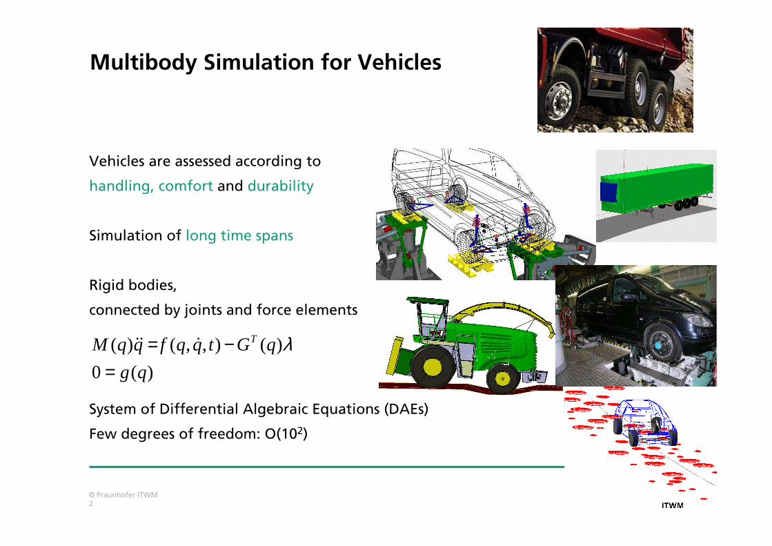
Multibody Simulation for Vehicles
Vehicles are assessed according to
handling, comfort and durability
Simulation of long time spans
Rigid bodies,
connected by joints and force elements
System of Differential Algebraic Equations (DAEs)
Few degrees of freedom: O(102)
( ) ( , , ) ( )
0 ( )
TM q q f q q t G q
g q
λ= −=ɺɺ ɺ
© Fraunhofer ITWM3
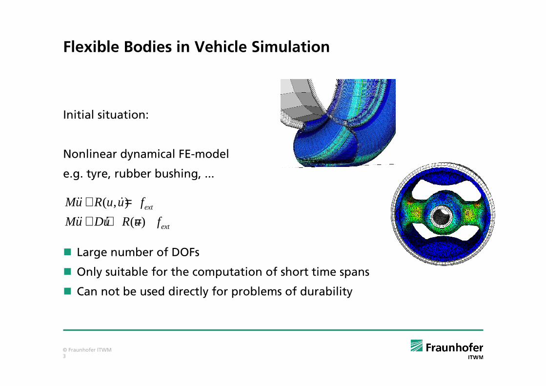
Flexible Bodies in Vehicle Simulation
Initial situation:
Nonlinear dynamical FE-model
e.g. tyre, rubber bushing, ...
� Large number of DOFs
� Only suitable for the computation of short time spans
� Can not be used directly for problems of durability
( , )
( )ext
ext
Mu R u u f
Mu Du R u f
+ =+ + =ɺɺ ɺ
ɺɺ ɺ
© Fraunhofer ITWM4
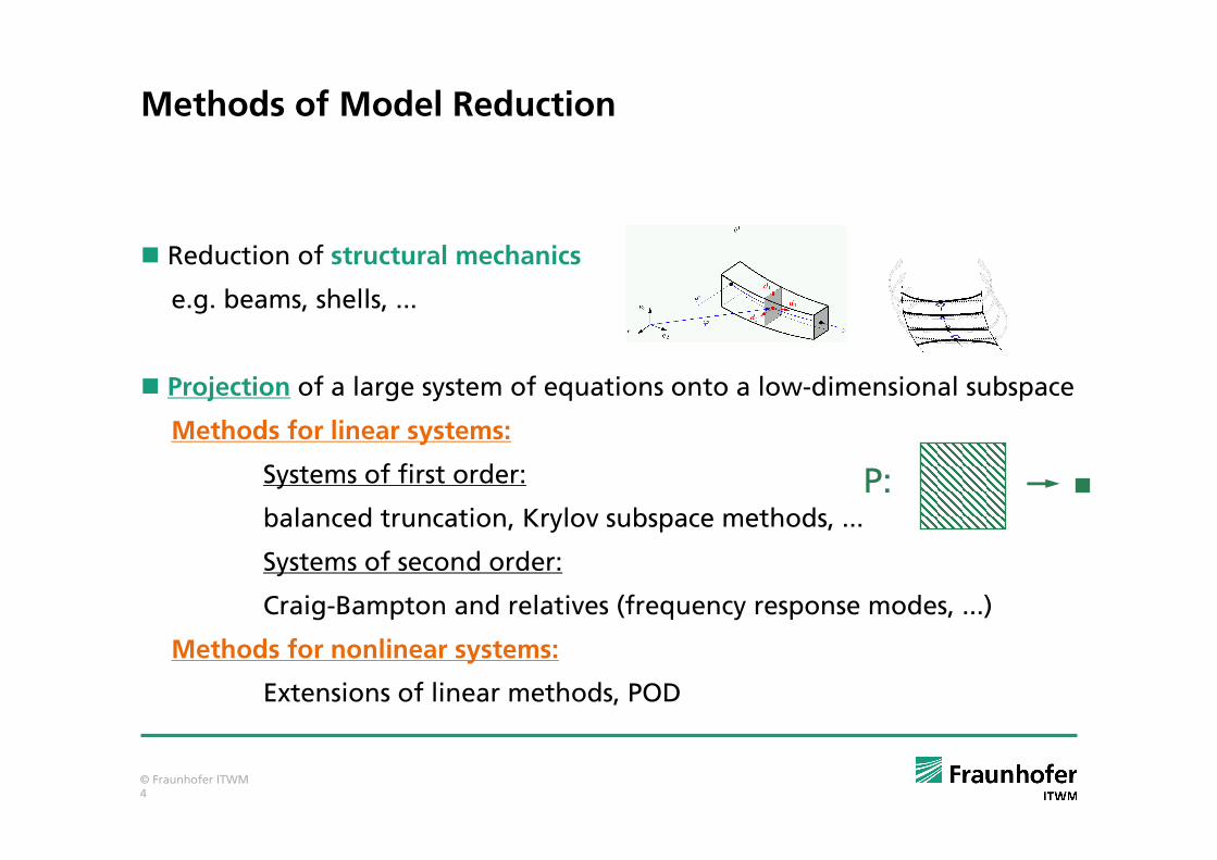
Methods of Model Reduction
� Reduction of structural mechanics
e.g. beams, shells, ...
� Projection of a large system of equations onto a low-dimensional subspace
Methods for linear systems:
Systems of first order:
balanced truncation, Krylov subspace methods, ...
Systems of second order:
Craig-Bampton and relatives (frequency response modes, ...)
Methods for nonlinear systems:
Extensions of linear methods, POD
P:

© Fraunhofer ITWM5
Linear Model Reduction – Craig-Bampton Method
“Classical” approach:
� Assume small deformations
� ODE system of flexible body can be linearised:
constant matrices!
Modal representation:
Reduction: Use only modes in relevant frequency range!
( )Mu Ku f t+ =ɺɺ
( ) ( ) ( )2
1
( , ) 0
ˆˆ ˆ ( )
ˆˆ ˆ, , ( ) ( )
M
k k k kk
T T T
u x t p t x with K M
Mp Kp f t
with M M diag K K diag f t f t
ϕ λ ϕ=
= ⋅ − ⋅ =
⇒ + =
= Φ Φ = = Φ Φ = = Φ
∑
ɺɺ
© Fraunhofer ITWM6
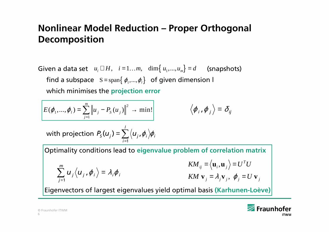
Nonlinear Model Reduction – Proper Orthogonal Decomposition
Given a data set (snapshots)
find a subspace of given dimension l
which minimises the projection error
with projection
{ }1, 1 , dim ,...,i mu H i m u u d∈ = =…
{ }1S span ,..., lϕ ϕ=
2
11
( ,..., ) ( ) min!m
l j S jj
E u P uϕ ϕ=
= − →∑ ijji δϕϕ =,
i
l
iijjS uuP ϕϕ∑
=
=1
,)(
Optimality conditions lead to eigenvalue problem of correlation matrix
Eigenvectors of largest eigenvalues yield optimal basis (Karhunen-Loève)
ii
m
jijj uu ϕλϕ =∑
=1
,
,
,
Tij i j
j j j j j
KM U U
KM Uλ ϕ
= =
= =
u u
v v v
© Fraunhofer ITWM7
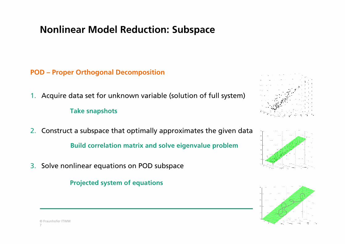
Nonlinear Model Reduction: Subspace
POD – Proper Orthogonal Decomposition
1. Acquire data set for unknown variable (solution of full system)
2. Construct a subspace that optimally approximates the given data
3. Solve nonlinear equations on POD subspace
Take snapshots
Build correlation matrix and solve eigenvalue problem
Projected system of equations
© Fraunhofer ITWM8
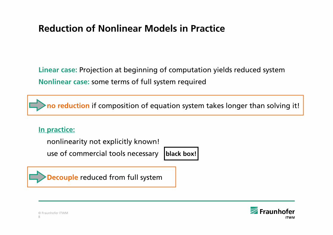
Reduction of Nonlinear Models in Practice
Linear case: Projection at beginning of computation yields reduced system
Nonlinear case: some terms of full system required
no reduction if composition of equation system takes longer than solving it!
In practice:
nonlinearity not explicitly known!
use of commercial tools necessary
Decouple reduced from full system
black box!
© Fraunhofer ITWM9
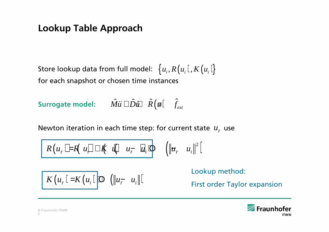
Lookup Table Approach
Store lookup data from full model:
for each snapshot or chosen time instances
Surrogate model:
Newton iteration in each time step: for current state use
( ) ˆˆ ˆ ˆextMu Du R u f+ + =ɺɺ ɺ
uτ
( ) ( ){ }, ,i i iu R u K u
( ) ( ) ( ) ( ) ( )2
i i i iR u R u K u u u u uτ τ τ= + − + Ο −
( ) ( ) ( )i iK u K u u uτ τ= + Ο −Lookup method:
First order Taylor expansion

© Fraunhofer ITWM10
Nonlinear Example Using Abaqus:Model Setup
2880 Degrees of freedom
Nonlinear material (Neo-Hooke)
Geometrical nonlinearities
( ) extMu Du R u f
D Mα+ + =
=
ɺɺ ɺ
© Fraunhofer ITWM11
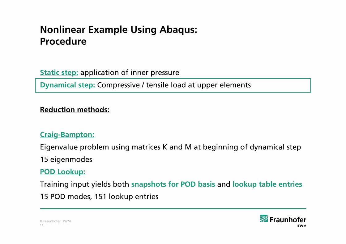
Nonlinear Example Using Abaqus:Procedure
Static step: application of inner pressure
Dynamical step: Compressive / tensile load at upper elements
Reduction methods:
Craig-Bampton:
Eigenvalue problem using matrices K and M at beginning of dynamical step
15 eigenmodes
POD Lookup:
Training input yields both snapshots for POD basis and lookup table entries
15 POD modes, 151 lookup entries
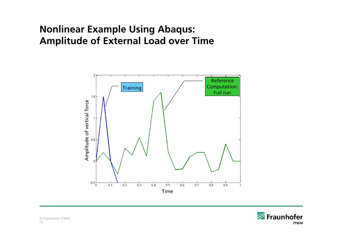
© Fraunhofer ITWM12
Training
Reference
Computation:
Full run
Am
plitu
de o
f vert
icalfo
rce
Time
Nonlinear Example Using Abaqus:Amplitude of External Load over Time

© Fraunhofer ITWM13
Nonlinear Example Using Abaqus:Training and Full Run – Deformations
Training Full run
© Fraunhofer ITWM14
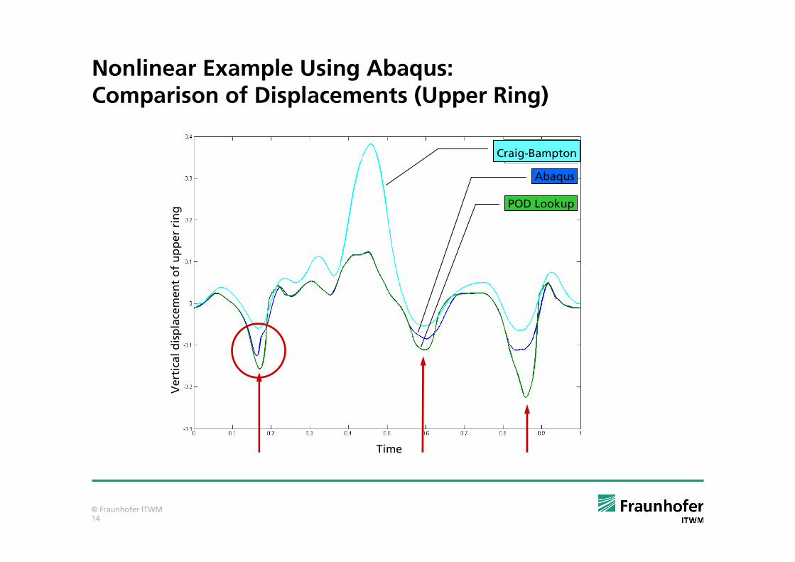
Nonlinear Example Using Abaqus:Comparison of Displacements (Upper Ring)
Vert
icaldis
pla
cem
entof
upper
ring
Time
Craig-Bampton
Abaqus
POD Lookup
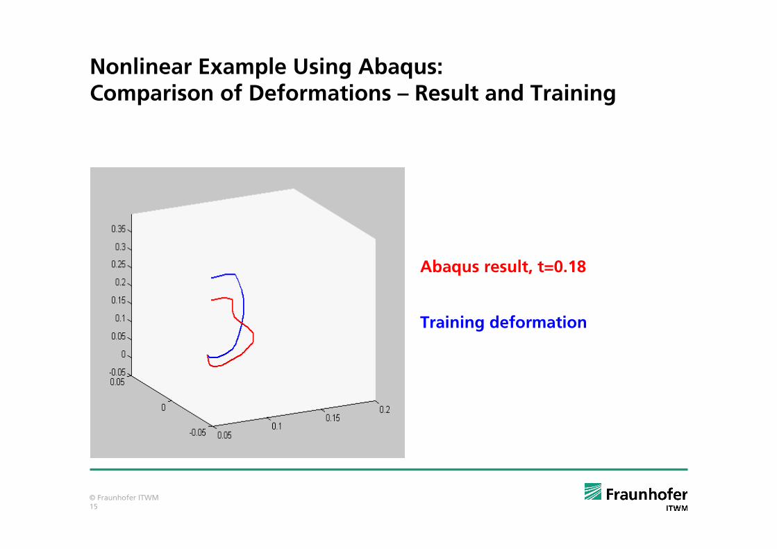
© Fraunhofer ITWM15
Nonlinear Example Using Abaqus:Comparison of Deformations – Result and Training
Abaqus result, t=0.18
Training deformation

© Fraunhofer ITWM16
Nonlinear Example Using Abaqus :Additional Training
Am
plitu
de o
f vert
icalfo
rce
Time
© Fraunhofer ITWM17
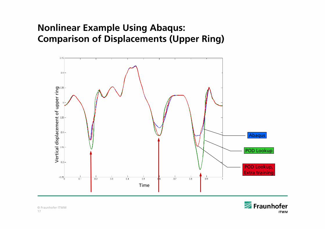
Nonlinear Example Using Abaqus:Comparison of Displacements (Upper Ring)
Vert
icaldis
pla
cem
entof
upper
ring
Time
Abaqus
POD Lookup
POD Lookup,
Extra training
© Fraunhofer ITWM18
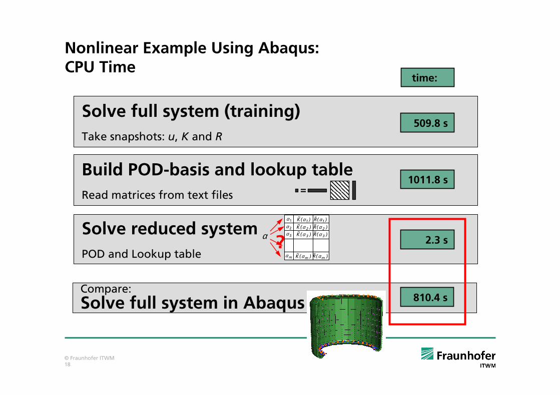
Nonlinear Example Using Abaqus:CPU Time
Solve full system (training)
Take snapshots: u, K and R
Build POD-basis and lookup table
Read matrices from text files
Solve reduced system
POD and Lookup table
=
509.8 s
2.3 s
1011.8 s
time:
)(R~
1α)(R
~2α
)(R~
mα
)(R~
3α
)(K~
1α)(K
~2α
)(K~
mα
)(K~
3α
1α
2α
mα
3αα?
Compare:
Solve full system in Abaqus 810.4 s

© Fraunhofer ITWM19
The BMBF Research Project SNiMoRed
Fraunhofer ITWM Dr. K. Dreßler, Dr. S. Herkt, U. Becker
Technische Universität Kaiserslautern Prof. Dr. B. Simeon, Prof. Dr. R. Pinnau
Martin-Luther-Universität Halle-Wittenberg Prof. Dr. M. Arnold
Universität der Bundeswehr München Prof. Dr. M. Gerdts
John Deere Werke Mannheim Dr. C. von Holst
AUDI AG Dr. O. Schlicht
Multidisziplinäre Simulation, nichtlineare Modellreduktion und
proaktive Regelung in der Fahrzeugdynamik
Funded by BMBF
© Fraunhofer ITWM20
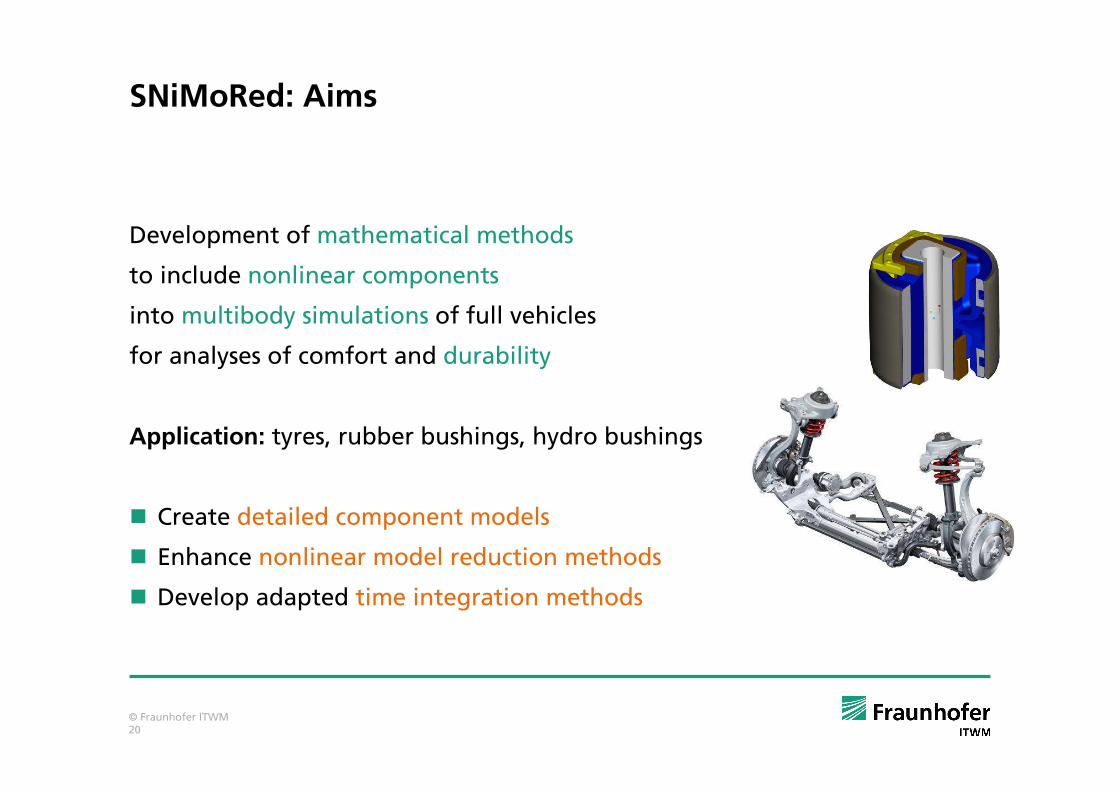
SNiMoRed: Aims
Development of mathematical methods
to include nonlinear components
into multibody simulations of full vehicles
for analyses of comfort and durability
Application: tyres, rubber bushings, hydro bushings
� Create detailed component models
� Enhance nonlinear model reduction methods
� Develop adapted time integration methods
© Fraunhofer ITWM21
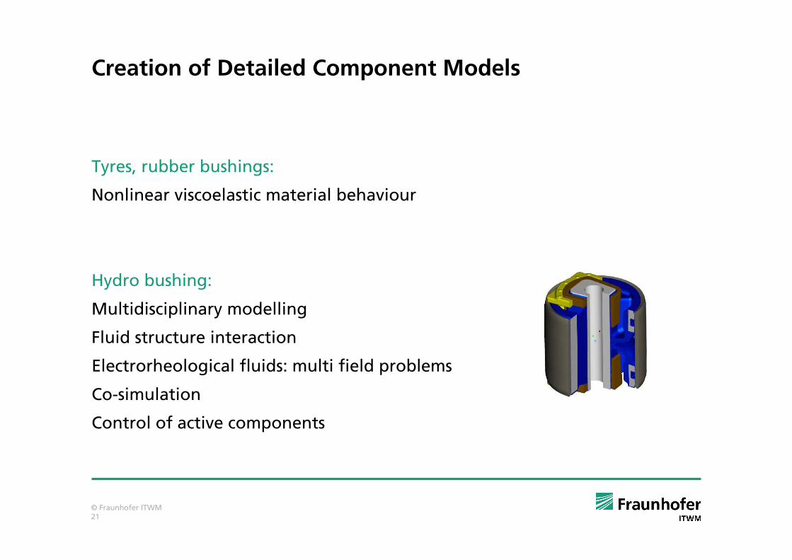
Creation of Detailed Component Models
Tyres, rubber bushings:
Nonlinear viscoelastic material behaviour
Hydro bushing:
Multidisciplinary modelling
Fluid structure interaction
Electrorheological fluids: multi field problems
Co-simulation
Control of active components

© Fraunhofer ITWM22
0 10 20 30 40−0.05
0
0.05
0.1
0.15
0.2
Zeit t [s]
F(t
) ,
x(t)
0 0.2 0.4 0.6 0.8 10
0.2
0.4
0.6
0.8
1
x(t) normiertF
(t)
norm
iert
0 10 20 30 40−0.5
0
0.5
1
1.5
2
Zeit t [s]
F(t
) ,
x(t)
Nonlinear Viscoelastic Material Behaviour
� Relaxation of stresses under given strain
� Description of material behaviour yields memory integral
R = Relaxation function with amplitude dependent coefficients
� Approach following Pipkin & Rodgers:
( ) ( )( )0
,td
F t R x t t s dsdt
= −∫
( )( ) ( ) ( )1 3 310 1 30 3, i i
t t
i ii i
R x t t C C e x t C C e x tτ τ− −
= + + +
∑ ∑
xa =0.2 xa = 2x(t)
F(t) F(t)
x(t)F(xa = 0.1)F(xa = 1)F(xa = 2)
© Fraunhofer ITWM23
Nonlinear Model Reduction and Inclusion into MBS
� Automatisation of the method: Optimal training excitation
� Enhancement of existing nonlinear model reduction methods:
� Contact
� Viscoelasticity, fluid-structure, …
� Adaptive meshing
� Error definition and estimate concerning durability
� Adaptation of time integration methods


