Numerical Continuation of Symmetric Periodic Orbits

Claudia Wulff

Department of Mathematics & Statistics

University of Surrey

Guildford GU2 7XH, United Kingdom

email: c.wulff@surrey.ac.uk

and

Andreas Schebesch

Fachbereich Mathematik und Informatik

Freie Universitat Berlin

14195 Berlin, Germany

email: schebesc@inf.fu-berlin.de

Dedicated to the memory of our dear friend and colleague Karin Gatermann

Abstract

The bifurcation theory and numerics of periodic orbits of general dynamical systems iswell developed, and in recent years there has been rapid progress in the development of abifurcation theory for symmetric dynamical systems. But there are hardly any results onthe numerical computation of those bifurcations yet. In this paper we show how spatio-temporal symmetries of periodic orbits can be exploited numerically. We describe methodsfor the computation of symmetry breaking bifurcations of periodic orbits for free groupactions and show how bifurcations increasing the spatiotemporal symmetry of periodic orbits(including period halving bifurcations and equivariant Hopf bifurcations) can be detectedand computed numerically. Our pathfollowing algorithm is based on a multiple shootingalgorithm for the numerical computation of periodic orbits via an adaptive Poincare sectionand a a tangential continuation method with implicit reparametrization.

AMS subject classification. 37G15, 37G40, 37M20, 65P30

Keywords. Numerical continuation, symmetry breaking bifurcations, symmetric periodic orbits

1

Contents

1 Introduction 3

2 Continuation of symmetric periodic orbits 4

2.1 Computation of single periodic orbits - single shooting method . . . . . . . . . . 42.2 Symmetries of periodic orbits and how to exploit them . . . . . . . . . . . . . . . 62.3 Multiple shooting approach . . . . . . . . . . . . . . . . . . . . . . . . . . . . . . 82.4 Continuation of nondegenerate periodic orbits . . . . . . . . . . . . . . . . . . . . 10

2.4.1 Single shooting method . . . . . . . . . . . . . . . . . . . . . . . . . . . . 102.4.2 Multiple shooting ansatz . . . . . . . . . . . . . . . . . . . . . . . . . . . . 11

2.5 Turning points . . . . . . . . . . . . . . . . . . . . . . . . . . . . . . . . . . . . . 12

3 Computation of flip down and flip up bifurcations 12

3.1 Detection and computation of period doubling bifurcations . . . . . . . . . . . . 133.1.1 Numerical detection of period doubling bifurcations . . . . . . . . . . . . 143.1.2 Computation of period doubling bifurcation points . . . . . . . . . . . . . 143.1.3 Computation of start off directions for the bifurcating branch . . . . . . . 15

3.2 Detection and computation of period halving bifurcations . . . . . . . . . . . . . 163.2.1 Detection of period halving bifurcations . . . . . . . . . . . . . . . . . . . 163.2.2 Computation of period halving bifurcation points and start off directions 17

3.3 Bifurcations of periodic orbits with Zp-symmetry . . . . . . . . . . . . . . . . . . 183.3.1 Flip pitchfork bifurcation . . . . . . . . . . . . . . . . . . . . . . . . . . . 183.3.2 Flip doubling bifurcation . . . . . . . . . . . . . . . . . . . . . . . . . . . 19

3.4 Numerical computation of symmetry breaking bifurcations . . . . . . . . . . . . . 193.4.1 Detection and computation of flip down bifurcations . . . . . . . . . . . . 193.4.2 Initialization of the bifurcating branch . . . . . . . . . . . . . . . . . . . . 19

3.5 Numerical computation of symmetry increasing bifurcations . . . . . . . . . . . . 203.5.1 Detection of flip up bifurcations . . . . . . . . . . . . . . . . . . . . . . . . 203.5.2 Computation of flip up points and start off tangents . . . . . . . . . . . . 21

4 Computation of equivariant Hopf points 21

4.1 Hopf bifurcations for non-symmetric systems . . . . . . . . . . . . . . . . . . . . 214.1.1 Detection of Hopf points along branches of periodic orbits . . . . . . . . . 224.1.2 Computation of Hopf bifurcations of non-symmetric systems . . . . . . . 22

4.2 Detection and computation of equivariant Hopf points . . . . . . . . . . . . . . . 244.2.1 Equivariant Hopf points . . . . . . . . . . . . . . . . . . . . . . . . . . . . 244.2.2 Detection of equivariant Hopf points . . . . . . . . . . . . . . . . . . . . . 254.2.3 Computation of equivariant Hopf bifurcations . . . . . . . . . . . . . . . . 25

5 Applications 31

5.1 The Lorenz model - comparison with AUTO and CONTENT . . . . . . . . . . . 315.2 Symmetry breaking bifurcations in coupled cells . . . . . . . . . . . . . . . . . . . 335.3 Electronic ring oscillator . . . . . . . . . . . . . . . . . . . . . . . . . . . . . . . . 35

Conclusion 39

2

1 Introduction

The bifurcation theory and numerics of periodic orbits of general dynamical systems is welldeveloped, see e.g. [1, 8, 13, 16, 17]. Frequently the considered problems possess certain sym-metries. Symmetries change the generic behaviour of a dynamical system dramatically, and inrecent years there has been rapid progress in the development of a bifurcation theory for periodicorbits of symmetric dynamical systems, see eg [9, 11, 18, 19, 24]. But there are hardly any resultson the numerical computation of those bifurcations yet. Gatermann and Hohmann [10] devel-oped numerical methods for the exploitation of symmetry and the computation of symmetrybreaking and symmetry increasing bifurcations of stationary solutions and implemented thosemethods in the mixed symbolic numerical code SYMCON. They treat finite symmetry groups.Cliffe et al [2] developed numerical methods for the computation of bifurcations of stationarysolutions in the case of continuous rotational symmetries.

In this paper we start a systematic theory on numerical bifurcation of symmetric periodicorbits by extending the methods of Gatermann and Hohmann [10] to periodic solutions. Weconsider a parameter dependent dynamical system

x = f(x, λ), f : Rn × R → R

n, (1.1)

which is equivariant with respect to a finite symmetry group Γ ⊂ GL(n), i.e.,

γf(x, λ) = f(γx, λ) ∀ γ ∈ Γ, x ∈ Rn, λ ∈ R.

In most parts of this paper we assume that Γ acts freely, i.e., γx 6= x for all γ 6= id andx ∈ Rn. We numerically continue periodic solutions with respect to the parameter λ exploitingpossible symmetries and computing symmetry breaking and symmetry increasing bifurcationsof those periodic orbits. For the computation of periodic orbits we employ the multiple shootingalgorithm presented by Deuflhard [5], which we briefly recall in Section 2.1. Section 2.2 isconcerned with the exploitation of spatial and spatio-temporal symmetries of periodic orbitsin the multiple shooting context. In Section 2.4 the aspect of continuation is added and thepathfollowing method of Deuflhard, Fiedler and Kunkel [7] is used for the continuation of periodicsolutions in the single and multiple shooting approach. A different method for the numericalcontinuation of periodic solutions with symmetry based on Fourier expansions has been presentedby Dellnitz [4].

In Sections 3 and 4 bifurcations of symmetric periodic orbits are treated. First symmetrybreaking and symmetry increasing bifurcations of periodic orbits are considered (Section 3) andthen equivariant Hopf bifurcations along periodic orbits (Section 4). In these sections numericaltechniques of Gatermann and Hohmann [10] are extended from stationary solutions to periodicsolutions.

Generic symmetry breaking bifurcations of periodic orbits of free group actions correspondto period doubling bifurcations in the space of group orbits, or equivalently, to period doublingbifurcations of the symmetry reduced Poincare map [18]. In Section 3.4 we show how suchsymmetry breaking bifurcations can be detected and computed numerically by extending thecorresponding methods for non-symmetric systems, c.f. Section 3.1.

We have also developed methods for the computation of bifurcations which increase thespatio-temporal symmetry of the periodic solution, in particular an algorithm for the compu-tation of period halving points which is based on the methods for computing period doublingbifurcation points, see Sections 3.2 and 3.5.

In Section 4 we derive methods for the detection of equivariant Hopf points along branchesof symmetric periodic orbits and present an extended system for the computation of equivariant

3

Hopf points. The main problem is how to deal with multiple Hopf eigenvalues forced by sym-metry. The issue of numerically dealing with multiple critical eigenvalues was treated by Cliffeet al [2] in the case of continuation of stationary solutions with continuous rotation symmetry.

The numerical methods we present have been implemented in the C code SYMPERCON [20].In Section 5, examples are presented to illustrate the performance of the developed algorithmictools. In Subsection 5.1 we use both SYMPERCON, AUTO [8] and CONTENT [17] for thecomputation of the period doubling cascade of the Lorenz equations to demonstrate the betterperformance of SYMPERCON. In Section 5.2 we compute symmetry breaking bifurcations ofperiodic orbits of four coupled cells. In Section 5.3 we show how oscillations of an electric circuitcan be computed efficiently by exploiting their spatio-temporal symmetry.

We partly follow the unpublished manuscripts [20, 22, 23]. For a description of the programSYMPERCON see [22, 20].

Acknowledgements

This paper is dedicated to the memory of Karin Gatermann who died on New Year’s Day 2005.She pioneered the use of symmetry methods in numerical bifurcation theory and introduced oneof us (CW) to this topic back in 1991. Karin gave us lots of valuable advice and encouragementand was a dear friend.

CW was partially supported by the Nuffield Foundation and by a European Union MarieCurie fellowship under contract number HPMF-CT-2000-00542, AS acknowledges funding bya European Union Marie Curie studentship at the Marie-Curie Training Site “University ofWarwick” during the academic year 2001/2002. CW thanks the Freie Universitat Berlin, inparticular the research group of Bernold Fiedler, for their hospitality during visits when partsof this paper were written. We both thank Mark Roberts for many helpful discussions and forinviting us to the Warwick Symposium on Geometric Mechanics and Symmetry in 2001/2002during which this project was started. Finally we acknowledge the EU-TMR network MASIEfor funding our participation in various summer schools, workshops and conferences.

2 Continuation of symmetric periodic orbits

In this section we review the multiple shooting method of Deuflhard [5] for the computation ofperiodic orbits, show how symmetries of periodic orbits can be exploited within the multipleshooting approach and present a continuation method for symmetric periodic orbits based onthe Gauss-Newton method.

2.1 Computation of single periodic orbits - single shooting method

In this subsection we briefly recollect the algorithm for the computation of periodic orbits of anautonomous ordinary differential equation (ODE)

x = f(x), f : Rn → R

n, (2.1)

which has been introduced in [5].Let Φt(·) be the flow of (2.1) and let x(t) = Φt(x

∗) be a periodic solution of (2.1) of periodT ∗, i.e., x(T ∗) = x∗. Then any time shifted solution x(t+ t0), t0 ∈ R, is also a periodic solution,because the system (2.1) is autonomous. All these solutions determine the same periodic orbit

P = Px(·) = {x(t), t ∈ R}.

4

In order to avoid this non-uniqueness a well known analytical technique is to fix a Poincaresection S = Sx∗ which is an (n − 1)-dimensional affine hyperplane transversal to the periodicorbit P at the point x∗, see e.g. [16]. Let us use the Poincare section orthogonal to the orbit

S = Sx∗ = x∗ + S′x∗ where S′

x∗ = span(f(x∗))⊥.

Then x∗ is a fixed point of the Poincare map (first return map) Π : S → S.

Definition 2.1 We say that a periodic orbit P with period T ∗ is non-degenerate if

DxΠ(x)|x=x∗ − id

is regular for x∗ ∈ P.

In this case x∗ is a locally unique fixed point of the Poincare map Π and a locally unique rootof the equation

F(x) := Π(x) − x = 0, where F : S → S.

Numerically one can either fix the phase by an additional phase condition, as described eg in[1, 16], or solve an underdetermined equation, as in [5]. We follow the latter approach andcompute a point x = x∗ on the periodic solution together with its period T = T ∗ by solving theunderdetermined equation F (y) = 0. Here F : Rn × R → Rn is given by

F (x, T ) = ΦT (x) − x = 0, where y = (x, T ). (2.2)

We solve (2.2) by an underdetermined Gauss-Newton method:

∆yk = −DF (yk)+F (yk),

yk+1 = yk + ∆yk,(2.3)

where DF (yk)+ denotes the Moore-Penrose pseudo-inverse of DF (yk). Remember that forA ∈ Mat(m, n), m ≤ n, rank A = m, x ∈ Rn, b ∈ Rm, x = A+b is defined by

Ax = b, x⊥ ker(A),

where ker(A) is the kernel of A. So x = A+b is the smallest in norm solution of Ax = b andhence the Newton correction ∆yk is the smallest solution of the underdetermined linear systemin (2.3).

The Jacobian DF (x, T ) of (2.2) in the solution (x∗, T ∗) is given by

DF (x∗, T ∗) = [− id +DxΦT∗(x∗), f(ΦT∗(x∗))] = [− id+DxΦT∗(x∗), f(x∗)]. (2.4)

Therefore a kernel vector tf of DF (y∗) at the solution point y∗ = (x∗, T ∗) is the tangenttf = (f(x∗), 0) to the trajectory.

Remark 2.2 This approach can be interpreted as computing periodic orbits in an adaptivePoincare section, which is approximately orthogonal to the periodic orbit: Since for the kernelvectors tk = (tkx, tkT ) of DF (yk) we have tk → tf as k → ∞, the Gauss-Newton iterate xk+1 =xk + ∆xk lies in the adaptive Poincare section Sxk = xk + span(tkx)⊥ ≈ x∗ + span(f(x∗))⊥.

If x∗ lies on a non-degenerate periodic orbit, i.e., if DxΠ(x∗) − id is regular, then by (2.4)the Jacobian DF (x∗, T ∗) is regular. Since this condition does not depend on the chosen pointx∗ on P we get the following convergence result:

Proposition 2.3 If the periodic orbit P through x∗ = ΦT∗(x∗) is non-degenerate then there isa tubular neighbourhood U of the periodic orbit P where there is no other periodic solution withperiod near T ∗ and which is such that the Gauss-Newton method (2.3) applied to (2.2) convergesfor initial data x ∈ U and T ≈ T ∗.

Before we review the extension of this basic shooting method to the multiple shooting contextwe show how symmetries of periodic orbits can be exploited numerically.

5

2.2 Symmetries of periodic orbits and how to exploit them

Let Γ ⊆ GL(n) be a finite group and let f be Γ-equivariant [11], ie:

f(γx) = γf(x) ∀ x ∈ Rn, γ ∈ Γ. (2.5)

This condition on the vectorfield (2.1) implies that if x(t) is a solution of the dynamical system(2.1) then also γ x(t) is a solution. Hence the flow Φt(·) of (2.1) is also Γ-equivariant: γΦt(x0) =Φt(γx0) for every γ ∈ Γ, x0 ∈ Rn.

For any x ∈ Rn the element γ x is called conjugate to x [11]. An element γ ∈ Γ is called asymmetry of x ∈ Rn if γx = x; the set of all symmetries of x (isotropy subgroup of x) is givenby K = Γx = {γ ∈ Γ | γx = x}. It can be seen easily that the vectorfield f of (2.1) maps thefixed point space of K

Fix(K) = {x ∈ Rn | γx = x ∀ γ ∈ K}

into itself. Thus we can restrict the ODE (2.1) to the fixed point space Fix(K) ' Rnred which hasa lower dimension nred ≤ n. In this way we obtain a symmetry reduced system fred : Rnred →Rnred which can be computed symbolically (see Gatermann, Hohmann [10]). The symmetrygroup acting on Fix(K) is N(K)/K where N(K) is the normalizer of K.

Remark 2.4 [11] If a finite group (or, more generally, a compact group) Γ acts linearly on thephase space X = Rn, i.e., if

γx := ϑ(γ)x, γ ∈ Γ, x ∈ X,

where ϑ : Γ → GL(n) is a homomorphism, then the phase space X = Rn can be decomposedinto a sum Rn = X1 ⊕X2 ⊕ . . .⊕Xl where the Xi are Γ-invariant vector spaces and can not bedecomposed into smaller Γ-invariant subspaces. Such vectorspaces Xi are called Γ-irreducibleand their corresponding reduced group actions ϑi := ϑ|Xi

are called irreducible representationsof the action of Γ on R

n. If a Γ-irreducible subspace X is also irreducible as a vectorspace overC, then its irreducible representation ϑ|X is called an absolutely irreducible representation. Ifit is reducible over C it is called a complex irreducible representation. We will encounter theconcept of irreducible representations in the computation of bifurcations, c.f. Section 4.2.

The spatial symmetries K of periodic solutions x(t) are those group elements γ ∈ Γ which leaveeach point on the periodic orbit invariant:

K := Γx(t) = {γ ∈ Γ | γx(t) = x(t) ∀ t}.

Since the flow Φt is Γ-equivariant the set of spatial symmetries K of a periodic solution x(t)does not depend on the time t. In addition to spatial symmetries there are also spatio-temporalsymmetries which leave the periodic orbit P := Px(·) invariant as a whole but not pointwise,i.e., the spatio-temporal symmetries of a periodic orbit P are given by

L := {γ ∈ Γ | γP = P}.

Each γ ∈ L corresponds to a phase shift Θ(γ) T ∗ of the T ∗-periodic solution x(t):

γ ∈ L ⇒ x(t) = γx(t + Θ(γ) T ∗), where Θ(γ) ∈ S1 ' R/Z. (2.6)

So spatio-temporal symmetries come in pairs (γ, Θ(γ)) ∈ Γ × S1. We define an action of thespatio-temporal symmetry group Γ×S1, where S1 = R/Z, on T ∗-periodic solutions x(t) of (2.1)as follows:

((γ, θ)x)(t) := γx(t + θT ∗), (γ, θ) ∈ Γ × S1. (2.7)

6

Note that Θ : L → R/Z is a group homomorphism with the spatial symmetries K as kernel andthat

L/K ≡ Z`, ` ∈ N, (2.8)

see [11]. The spatial symmetries of periodic solutions can be exploited by restriction onto thefixed point space Fix(K), i.e., by using a symmetry reduced system fred : Fix(K) → Fix(K).

From now on we assume that the spatial symmetry K of the periodic orbit is trivial. Thenthe spatio-temporal symmetries of the periodic orbit form a finite cyclic group L = Z`. Inbifurcation theory the spatio-temporal symmetries of periodic orbits are taken into account bystudying the reduced Poincare map. It was first introduced by Fiedler [9] and later used byLamb, Melbourne and Wulff [18, 19] in order to classify symmetry breaking bifurcations ofperiodic orbits, see also Section 3. Let α ∈ L = Z` be that element in L that corresponds to thesmallest possible non-zero phase shift T ∗/`:

α x(t +T ∗

`) = x(t) ∀ t. (2.9)

We call this spatio-temporal symmmetry the drift symmetry of the periodic orbit [25]. Forx∗ ∈ P define the Poincare section as usual by S = x∗ + span(f(x∗))⊥. Then the reducedPoincare map is defined as

Πred = αΠ, Π : S → α−1 S, (2.10)

where α is the drift symmetry of the periodic orbit, i.e., satisfies (2.9), and Π maps x ∈ S intothe point where the positive semi-flow through x first hits α−1 S [9]. The fixed point equationΠred(x) = x or, equivalently, the equation

F(x) = Πred(x) − x = 0, where F : S → S,

then determines periodic orbits with spatio-temporal symmetry L. Note that in the case oftrivial symmetry ` = 1, α = id, the reduced Poincare map Πred becomes the standard Poincaremap Π introduced in Section 2.1. In order to numerically exploit spatio-temporal symmetrieswe proceed as in Section 2.1: Each point x on a T -periodic orbit with drift symmetry α satisfiesthe underdetermined equation

F : Rn × R → R

n, F (x, T ) = αΦT`(x) − x = 0. (2.11)

This system is analogous to the corresponding underdetermined system (2.2) in the case of trivialsymmetry and reduces to it in the case α = id, ` = 1. It can also be solved by a Gauss-Newtonmethod. Note that it suffices to compute the flow Φt(·) and the Wronskian matrix DxΦt(·) onlyup to time T

` instead of T , which is a remarkable reduction of the computational cost in thecase of high spatio-temporal symmetry. In a solution point (x∗, T ∗) we have

DF (x∗, T ∗) = [αDxΦT∗

`(x∗) − id,

1

`f(αΦT∗

`(x∗))] = [αDxΦT∗

`(x∗) − id,

1

`f(x∗)], (2.12)

analogous to the case of trivial symmetry, c.f. (2.4). In particular DF (x∗, T ∗) is closely relatedto DxF(x∗) = DxΠred(x)|x=x∗ − id. We extend the definition of non-degeneracy to symmetricperiodic orbits as follows:

Definition 2.5 We say that a symmetric periodic orbit P with drift symmetry α is non-degenerateif DΠred(x∗) − id is regular for x∗ ∈ P where Πred is from (2.10).

From (2.12) we conclude that DF (x∗, T ∗) in the periodic orbit is regular if and only if theperiodic orbit is non-degenerate, and so we get the following proposition which is analogous toProposition 2.3:

7

Proposition 2.6 If the symmetric periodic orbit through x∗ = αΦT∗

`(x∗) is non-degenerate in

the sense of Definition 2.5 then there is a tubular neighbourhood U about the periodic orbit Pthrough x∗ with the property that there is no other periodic orbit with symmetry L and periodnear T ∗ in U and which is such that the Gauss-Newton method (2.3) applied to (2.11) convergesfor initial values x ∈ U , T ≈ T ∗.

2.3 Multiple shooting approach

In order to numerically compute unstable symmetric periodic solutions we use the just describedalgorithm in the multiple shooting context (c.f. [5]): we compute k points on a periodic orbitwith spatio-temporal symmetry L = Z`, trivial isotropy and drift symmetry α by solving theunderdetermined equation

F (x1, . . . , xk, T ) = 0, F : RN → R

M , (2.13)

where N = M + 1 = kn + 1, 0 = s1 < . . . < sk+1 = 1 is a partition of the unit interval,∆si = si+1 − si for i = 1, . . . k, and

Fi(x1, . . . , xk, T ) =

{Φ∆siT

`

(xi) − xi+1 for i = 1, . . . , k − 1,

αΦ∆skT

`

(xk) − x1 for i = k.(2.14)

The linear systems which arise in the Gauss-Newton method are of the form Jy = b, wherey = (x, T ) ∈ Rnk+1, x = (x1, . . . , xk), b = (b1, . . . , bk),

J = DF (x, T ) =

G1 − id g1

G2 − id g2

. . .. . .

...Gk−1 − id gk−1

− id Gk gk

= [G, g], (2.15)

where G is an (nk, nk)-matrix, g an nk-vector, and

Gi = DxΦ∆siT

`

(xi), i = 1, 2, . . . , k − 1,

Gk = αDxΦ∆skT

`

(xk),

gi = DT Fi(x, T ) = DT Φ∆siT

`

(xi) = ∆si

` f(Φ∆siT

`

(xi)), i = 1, . . . , k − 1,

gk = ∆sk

` αf(Φ∆skT

`

(xk)).

We have

Jy = b ⇔ [G, g]

(x

T

)= b ⇔ Gx = b − gT,

so we can apply Gaussian block elimination to G to solve these linear systems. This yields thefollowing algorithm:

1.) Compute the condensed right hand side

bc := C(G, b, k) = bk + Gkbk−1 + · · · + Gk · · ·G2b1.

2.) Compute the condensed matrix [Gc, gc] with

Gc := Gk · · ·G1, gc := C(G, g, k). (2.16)

8

3.) Compute a solution of the condensed system [Gc − id, gc](x1

T

)= bc, e.g.

(x1

T

)= [Gc − id, gc]

+ bc,

using QR-decomposition.

4.) Compute x via the explicit recursion

xi = Gi−1xi−1 − bi−1 + gi−1T for i = 2, . . . , k. (2.17)

We have now obtained a solution y = J−b where y = (x, T ) and J− is an outer inverse of J . Inorder to compute the solution J+b where J+ is the Moore-Penrose pseudo-inverse of J we haveto add one more step:

5.) Compute the kernel vector t = (tx, tT ) of J , where tx = (t1, t2, . . . , tk). Starting from atangent of the condensed system

(t1tT

)

[Gc − id, gc]

(t1tT

)= 0

we obtain a tangent t of the whole system by

ti = Gi−1ti−1 + gi−1tT for i = 2, . . . , k.

In the end we project y → y − 〈y,t〉〈t,t〉 t.

An easy computation shows that in a solution point y∗ = (x∗, T ∗) we have

[Gc − id, gc] = [αDxΦT∗

`(x∗

1) − id,1

`f(x∗

1)], (2.18)

so the condensed matrix Ec := [Gc − id, gc] equals the Jacobian (2.12) of the single shootingapproach in the point x∗

1. The Jacobian J is regular iff [Gc − id, gc] is regular. Hence we get thefollowing result which is analogous to Proposition 2.6:

Theorem 2.7 The Jacobian J of the multiple shooting system (2.13) is regular at the symmetricperiodic orbit if and only if the periodic orbit is non-degenerate in the sense of Definition 2.5. Inthis case the Gauss-Newton method (2.3) applied to (2.13) converges for sufficiently good initialdata.

Remarks 2.8

a) The approach for symmetry exploitation in the multiple shooting approach can be trans-ferred to collocation methods (used in AUTO and CONTENT [8, 17]) since collocation canbe viewed as a special case of a multiple shooting method where the number of grid pointscorresponds to the number of multiple shooting points k and the initial value problemsolver consists of only one integration step of a collocation method. The advantage of themultiple shooting approach is that it allows the use of adaptive order and stepsize initialvalue problem solvers for the computation of the flow Φt(x) and the Wronskians DxΦt(x)which we use for the evaluation of F rsp. DF , like the extrapolation codes of Deufhard [6].These techniques have been implemented in the code SYMPERCON [22, 20], see Section5.1 for a comparison with AUTO and CONTENT.

9

b) Note that in the program packages AUTO and CONTENT [8, 17] a phase condition is usedto obtain a unique periodic orbit, whereas we solve an underdetermined equation for theperiodic orbit. Since we use the Moore-Penrose pseudo-inverse to compute the correctionsof the Gauss-Newton method ∆yk = −DF (yk)+F (yk), we have ∆yk⊥ ker(DF (yk)). Here

ker(DF (yk)) ≈ ker(DF (y∗)) = span(tf ),

wheretf = (f(x∗

1), . . . , f(x∗k), 0, 0). (2.19)

The condition ∆yk⊥ ker(DF (yk)) is therefore an ”adaptive phase condition” which is suchthat the correction ∆yk is the smallest solution of the equation for the Newton correctionsDF (yk)∆yk = −F (yk), c.f. Remark 2.2.

c) Dellnitz [3, 4] computes symmetric periodic orbits by a Galerkin ansatz based on Fouriermodes. This method is effective near Hopf bifurcations since in this situation periodicorbits can be approximated by few Fourier modes.

2.4 Continuation of nondegenerate periodic orbits

In this section we show how the pathfollowing method for stationary solutions described in [7] canbe extended to the case of symmetric periodic solutions. We consider the parameter dependentΓ-equivariant dynamical system x = f(x, λ) from (1.1) again and first look at stationary solutionsof (1.1),

f(y) = 0, f : Rn+1 → R

n, y = (x, λ). (2.20)

If y∗ = (x∗, λ∗) is a stationary solution and Dyf(y) is regular at y∗ then (2.20) locally defines asolution branch. We apply the tangential continuation method based on implicit reparametriza-tion presented in [7] to compute this solution branch. By writing y = (x, λ) we want to expressthat the parameter λ does not play any extraordinary role so that turning points can be treatedeasily. The pathfollowing algorithm works as follows: if a solution y∗ is given a new guess y iscomputed by setting y = y∗ + ε t(y∗) where t(y) is the normalized kernel vector of Dyf(y), andhence the continuation tangent, and ε is a suitably chosen stepsize. Then an underdeterminedGauss-Newton method as in (2.3) is used for the iteration from the guess y back to the solutionpath. The stepsize control is described in [7]. We now show how to apply this continuationmethod to symmetric periodic orbits.

2.4.1 Single shooting method

In the case of symmetric periodic solutions we want to compute fixed points of the parameterdependent reduced Poincare map Πred : S × R → S

Πred(x, λ) = x ⇔ F(x, λ) := Πred(x, λ) − x = 0, (2.21)

or, equivalently, solutions of the parameter dependent nonlinear equation

F(x, λ) = 0, F : S × R → S.

We can in principle apply the above described continuation method to this equation. Thecontinuation tangent in a solution point (x∗, λ∗) is simply the kernel vector t∗F of DF(x∗, λ∗).But in the numerical realization of this idea we want to use the method of adaptive Poincaresections of Sections 2.1, 2.2, c.f. Remark 2.2. So we again introduce the period as a new variableand solve (in the single shooting approach) the underdetermined equation

F : Rn+2 → R

n, F (x, T, λ) = αΦT`(x, λ) − x = 0, (2.22)

10

by a Gauss-Newton procedure. Now the kernel ker(DF ) of DF is two-dimensional. In a solutionpoint (x∗, λ∗) one kernel vector of DF is the tangent to the periodic orbit

tf = (f(x∗, λ∗), 0, 0) ∈ ker(DF (x∗, T ∗, λ∗)).

We want to determine the continuation tangent t∗ in such a way that it corresponds to thetheoretical tangent vector t∗F . First the continuation tangent has to be in the kernel of DF ,and second the continuation tangent should lie in the Poincare section S. Since we choose thePoincare section orthogonal to the orbit, this leads to the conditions

t∗ ∈ ker(DF ), t∗ ⊥ tf . (2.23)

The Jacobian in the solution point (x∗, T ∗, λ∗) is given by

DF (x∗, T ∗, λ∗) = [αDxΦT∗

`(x∗, λ∗) − id,

1

`f(x∗, λ∗), αDλΦT∗

`(x∗, λ∗)], (2.24)

and therefore we get the following proposition, analogous to Proposition 2.6:

Proposition 2.9 Let x∗ lie on a T ∗-periodic orbit P of (1.1) with symmetry L = Z` and driftsymmetry α. Then the Jacobian DF (x∗, T ∗, λ∗) is regular if and only if

DF(x∗, λ∗) = [DxF(x∗, λ∗), DλF(x∗, λ∗)] = [DxΠred(x∗) − id, DλΠred(x∗)] (2.25)

is regular. In this case the path of periodic solutions given by (2.21) is locally unique in thefollowing sense: there is a tubular neighbourhood U of the periodic orbit P such that everyperiodic solution x(t) in this neighbourhood with period T close to T ∗, parameter λ close to λ∗

and drift symmetry α lies on the path of periodic solutions defined by (2.21). Moreover theGauss-Newton method (2.3) applied to (2.22) converges to a periodic solution on this path for

initial data x ∈ U , T ≈ T ∗, λ ≈ λ∗.

Note that for non-degenerate periodic orbits the condition of Proposition 2.9 is always satisfied,but it also holds in a turning point bifurcation, see Section 2.5.

2.4.2 Multiple shooting ansatz

In the multiple shooting approach we solve the parameter dependent equation

F (x1, . . . , xk, T, λ) = 0, F : Rnk × R × R → R

nk, (2.26)

where F is as in (2.14). Nearly everything carries over from Section 2.3, we just have one morecolumn in the Jacobian consisting of the parameter derivatives

Pi = DλΦ∆siT

`

(xi, λ), i = 1, . . . , k − 1, Pk = αDλΦ∆skT

`

(xk , λ).

Therefore, to solve the linear equations Jy = b, y = (x1, . . . , xk, T, λ), we have to compute anadditional condensed vector (step 1 in the Gaussian block elimination algorithm), namely

pc := C(P ) = Pk + GkPk−1 + · · · + Gk · · ·G2P1.

The condensed matrix in steps 2 and 3 is of the form [Gc − id, gc, pc], the recursion (step 4) hasto be modified to

xi = Gi−1xi−1 − bi−1 + gi−1T + Pi−1λ for i = 2, . . . , k,

11

and in step 5 we compute an orthonormal basis of the 2-dimensional kernel of J and project thepreliminary solutions y = J−b onto the orthogonal complement of this kernel.

As can be seen from the Gaussian block elimination, J has full rank if the condensed matrixEc := [Gc − id, gc, pc] has full rank. A simple computation shows that the matrix Ec equals theJacobian of the single shooting approach (2.24). Thus the Gauss-Newton method (2.3) appliedto the multiple shooting system of equations (2.26) converges under the same conditions to asolution as the Gauss-Newton method of the single shooting method, namely if the assumptionsof Proposition 2.9 are satisfied.

As in the case of the single shooting method, we choose the continuation tangent t∗ as thekernel vector of DF (y∗) (with F from (2.26)) which is orthogonal to tf from (2.19).

2.5 Turning points

Before we come to the detection and computation of bifurcations of symmetric periodic orbitsin Sections 3 and 4 we first consider turning points of symmetric periodic orbits. We saw thatperiodic orbits are solutions of the equation F(x, λ) = 0 where F is as in (2.21). Turning pointsare characterized by the condition that DxF(x∗, λ∗) from (2.25) is singular, but that DF(x∗, λ∗)has full rank. In this case the solution path (x(s), λ(s)), of (2.21), s ∈ R, x(0) = x∗, λ(0) = λ∗,satisfies λ′(0) = 0. Generically λ′′(0) 6= 0 so that the solution path has a turning point in λ.Turning points can be detected by a change of sign of the λ-component t∗λ of the continuationtangent t∗ of the periodic solution provided this test is done after the tests of other bifurcations.This ordering of the monitoring tests for bifurcations is important, because, as we will see inSections 3.2, 3.5 and 4, a change of sign of the λ-component t∗λ of the continuation tangent t∗

also occurs at flip up bifurcations and Hopf points along periodic orbits.A turning point between two points y(0) = (x(0), T (0), λ(0)) and y(1) = (x(1), T (1), λ(1)) with

continuation tangents t(0), t(1) respectively is detected if

t(0)λ t

(1)λ < 0.

The λ-component of the turning point is then computed by Hermite interpolation exactly inthe same way as in the case of stationary solutions, see [7]: We construct a cubic polynomialy(τ) = (x(τ), T (τ), λ(τ)), where y : [0, 1] → RN , over the line y(0) + τ(y(1) − y(0)), τ ∈ [0, 1],such that

y(0) = y(0), y′(0) = ‖y(1)−y(0)‖2

〈y(1)−y(0),t(0)〉t(0),

y(1) = y(1), y′(1) = ‖y(1)−y(0)‖2

〈y(1)−y(0),t(1)〉t(1),

(2.27)

and solve the quadratic equation dλdτ (τ) = 0 for its unique root τ ∈ [0, 1]. We then take the value

y = y(τ ) of the Hermite polynomial at τ as initial guess for a Gauss-Newton iteration. Theperiodic solution y∗ obtained in this way is accepted as turning point if

|t∗λ| < tol

where t∗ is the continuation tangent at y∗ and tol is the required accuracy of the computation.

Otherwise we replace y(0) or y(1) by y∗ so that t(0)λ t

(1)λ < 0 and repeat the procedure.

3 Computation of flip down and flip up bifurcations

In this section we show how generic bifurcations of symmetric periodic orbits to other periodicorbits can be computed numerically. This involves the detection and numerical computation ofbifurcation points and the computation of the start off directions for the bifurcating branches.

12

We only have to follow non-conjugate branches and distinguish between two types of symmetrychanging bifurcations: there are symmetry increasing bifurcations which lead to a super groupof the symmetry group of the original solution, i.e., the bifurcating solutions possess more sym-metry, and we have symmetry breaking bifurcations which lead to a subgroup of the symmetrygroup of the original solution.

In this section we only treat bifurcations from periodic orbits to periodic orbits, not Hopfbifurcations (from periodic orbits to stationary solutions) - we will treat these in the nextsection. Such bifurcations have been classified by Fiedler [9] in the case of cyclic symmetrygroups. Bifurcations of periodic orbits in systems with arbitrary finite symmetry group wereclassified by Lamb and Melbourne [18], see also [19].

In this paper we assume that the symmetry group of the dynamical system is discrete andthat the isotropy K of the periodic orbit is trivial, i.e., we restrict the dynamical system to thecorresponding fixed point space Fix(K). In other words, we do not treat bifurcations to periodicorbits with smaller or bigger isotropy group K. The methods we present extend the techniques ofGatermann and Hohmann [10] for the numerical computation of symmetry changing bifurcationsof stationary solutions to the case of periodic solutions. In particular, the symmetry monitoringfunctions which are used for the detection of symmetry changing bifurcations are related tothose used in [10].

Generic bifurcations of periodic orbits with trivial isotropy to other periodic orbits are causedby a period doubling (flip down) or period halving (flip up) bifurcation of the reduced Poincaremap [18, 19]. We start with generic bifurcations without symmetry where the ODE (1.1) is notassumed to be equivariant.

3.1 Detection and computation of period doubling bifurcations

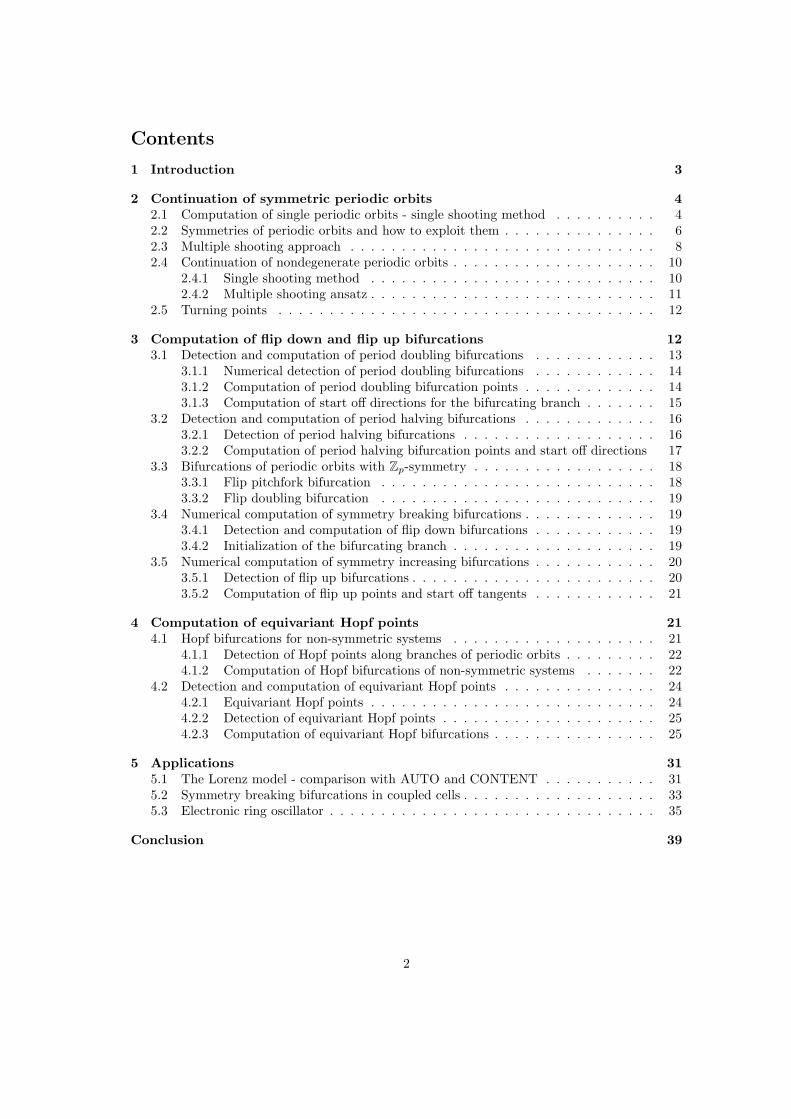
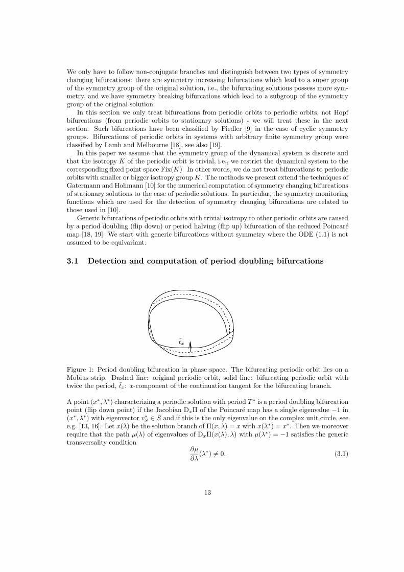
tx

Figure 1: Period doubling bifurcation in phase space. The bifurcating periodic orbit lies on aMobius strip. Dashed line: original periodic orbit, solid line: bifurcating periodic orbit withtwice the period, tx: x-component of the continuation tangent for the bifurcating branch.

A point (x∗, λ∗) characterizing a periodic solution with period T ∗ is a period doubling bifurcationpoint (flip down point) if the Jacobian DxΠ of the Poincare map has a single eigenvalue −1 in(x∗, λ∗) with eigenvector v∗

S ∈ S and if this is the only eigenvalue on the complex unit circle, seee.g. [13, 16]. Let x(λ) be the solution branch of Π(x, λ) = x with x(λ∗) = x∗. Then we moreoverrequire that the path µ(λ) of eigenvalues of DxΠ(x(λ), λ) with µ(λ∗) = −1 satisfies the generictransversality condition

∂µ

∂λ(λ∗) 6= 0. (3.1)

13

Under these assumptions (x∗, λ∗) is a pitchfork bifurcation point of the map

F(x, λ) = Π(Π(x, λ), λ) − x = 0, (3.2)

see [13, 16]. The normal form of this bifurcation is

f(z, λ) = z3 − λz. (3.3)

By a Lyapounov-Schmidt reduction (3.2) can be reduced to a scalar equation in z = 〈x−x∗, v∗S〉.After a suitable change of coordinates this scalar equation takes the form (3.3), up to order 3,see [13, 16]. The vector tF = (v∗S , 0) is the tangent vector of the bifurcating branch in (x∗, λ∗).The bifurcating periodic orbits correspond to fixed points of Π2 and hence have approximatelytwice the period of the original periodic solution. They lie on a Mobius strip around the originalperiodic orbit, see Figure 1. The map F is Z2-equivariant where the nonlinear Z2-action is givenby the Poincare map (x, λ) → (Π(x), λ) (in the normal form (3.3) this Z2-symmetry becomesz → −z). So a period doubling bifurcation is a Z2-symmetry breaking bifurcation of equilibria of

F . If we consider the T -periodic solutions on the original branch as T -periodic, where T := 2T ,the original branch has temporal Z2-symmetry for the action of the spatio-temporal symmetrygroup Γ × R given by (2.7):

(id, θ)x(t) = x(t + θT ) = x(t) for θ = 1/2,

and the branching solutions are not Z2-symmetric. So we see that even in the case of a triv-ial symmetry group Γ = {id} the period doubling bifurcation corresponds to a Z2-symmetrybreaking bifurcation as the phase shift symmetry (temporal symmetry) of the periodic orbit isbroken.

In the following we briefly describe how to numerically detect and compute period doublingbifurcations in non-symmetric systems. We adapt standard techniques used in the context ofcollocation methods [1, 8, 17] to our approach for the computation of periodic orbits as solutionsof underdetermined systems, as described in Section 2. In Section 3.5 we show how to adaptthese methods to the numerical computation of symmetry breaking bifurcations of symmetricperiodic orbits.

3.1.1 Numerical detection of period doubling bifurcations

Period doublings can be detected by a change of sign of

d(λ) := det(DxΦT∗(x∗, λ∗) + id)

which occurs due to the transversality condition (3.1). The matrix DxΦT∗(x∗, λ∗) is computedin the single shooting approach to obtain DF (x∗, T ∗, λ∗), see (2.4), and also in the multipleshooting approach in the computation of the condensed matrix Gc, see (2.18) with ` = 1 andα = id.

3.1.2 Computation of period doubling bifurcation points

If a period doubling point has been detected it can be computed by use of linear interpolationand a Gauss-Newton procedure to iterate back to the solution path: If there is a period doublingpoint between two consecutively computed periodic solutions y(0) and y(1) then

d(λ(0))d(λ(1)) < 0.

14

By linear interpolation of the two points (λ(0), d(λ(0))) and (λ(1), d(λ(1))) we obtain a point (λ, 0)

which gives us an approximation for the parameter value λ of the bifurcation point. Linearinterpolation between the points y(0) and y(1) provides a first guess y with parameter λ for theperiod doubling point. This guess is then iterated back to a point y∗ on the solution path by aGauss-Newton procedure. If

‖y∗ − y‖ ≤ tol,

y∗ is accepted as period doubling point. If not, then either y(0) or y(1) is replaced by y∗, suchthat the condition d(λ(0))d(λ(1)) < 0 is satisfied, and the procedure is repeated.

Doubling the number of multiple shooting points for the bifurcating branch If wefix the number of multiple shooting points on the bifurcating branch of 2T -periodic solutions,then after some period doubling bifurcations the multiple shooting method is likely to divergebecause the initial number of multiple shooting points will not be appropriate for a periodicsolution with a much higher period than the original period. Therefore it is preferable tocompute the bifurcating branch of periodic orbits with twice as many multiple shooting points,i.e., to set k = 2k as the number of multiple shooting points of the bifurcating branch. Thebifurcation point y = (x1, . . . , xk , T , λ) on the bifurcating branch is given by

xi = x∗i , xi+k = x∗

i for i = 1, . . . , k, T = 2T ∗, λ = λ∗,

and the multiple shooting nodes si, i = 0, 1, . . . , k, of the bifurcating branch are set to

si =si

2, si+k =

1 + si

2, i = 1, . . . , k.

3.1.3 Computation of start off directions for the bifurcating branch

After a period doubling bifurcation point has been found the start off direction for the bifurcatingbranch has to be computed. The continuation tangent of the original periodic branch is just theusual continuation tangent. The start off direction for the bifurcating branch is computed asfollows:

Single shooting ansatz We first consider the single shooting approach: we want the startoff direction for the bifurcating branch of periodic orbits to be orthogonal to the T ∗-periodicorbit, so that it lies in the Poincare section S. In S ×R the tangent of the bifurcating branch inthe bifurcation point should be the vector tF = (v∗S , 0) where v∗

S is the eigenvector of DxΠ(x∗)to the eigenvalue −1, see above. It can be computed by projecting the kernel vector v∗ ofDxΦT (x∗, λ∗) + id onto the orthogonal complement of the tangent f(x∗) to the periodic orbitthrough x∗: Let

tx = v∗ −〈v∗, f(x∗)〉

〈f(x∗), f(x∗)〉f(x∗). (3.4)

Then we taket = (tx, tT , tλ) = (tx, 0, 0)

as the start off direction for the bifurcating periodic solutions. In phase space the bifurcatingperiodic solutions lie on a Moebius band in the middle of which is the original T ∗-periodicsolution. The start off direction is tangential to the Moebius band and orthogonal to the originalsolution (see Figure 1).

15

Multiple shooting ansatz As preliminary tangent vector v∗1 of the bifurcating branch for the

first multiple shooting point we choose the eigenvector of Gc + id to −1 where Gc ≈ DxΦT∗(x∗)is the condensed matrix, see (2.16, 2.18). As preliminary tangent start off directions at themultiple shooting points x∗

2,. . . , x∗k we take

v∗j = Gjv∗j−1, j = 2, . . . , k.

The first nk components of the start off tangent t of the bifurcating branch in the multiple shoot-ing approach are then obtained by projecting v∗ = (v∗1 , . . . , v∗k) to the orthogonal complementof the vector tf = (f(x∗

1), . . . , f(x∗k)).

Since the number of multiple shooting points is doubled on the bifurcating branch (see Section3.1.2), this gives us only the first half of the x-component

tx = (t1, t2, . . . , tk, tk+1, . . . , t2k)

of the start off tangent t = (tx, 0, 0) of the bifurcating branch. The whole x-component of t isobtained by copying the first half into the second half and multiplying it with −1, i.e.,

tk+i = −ti, i = 1, . . . k. (3.5)

As in the single shooting approach we have tT = tλ = 0.

3.2 Detection and computation of period halving bifurcations

In this section we describe an algorithm for the detection and computation of period halvingbifurcations (flip up points) along branches of periodic orbits. Again, we assume that the sym-metry group Γ of the dynamical system (1.1) is trivial.

3.2.1 Detection of period halving bifurcations

Period halvings can be detected as follows: for a solution point y = (x1, . . . , xk, T, λ) of (2.26)we compute

u(y) := ΦT2(x1, λ) − x1 = xj − x1.

Here one multiple shooting node sj is set to sj = 1/2 so that no additional initial value problemhas to be solved.

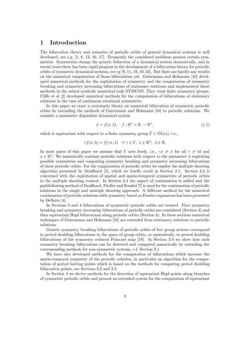
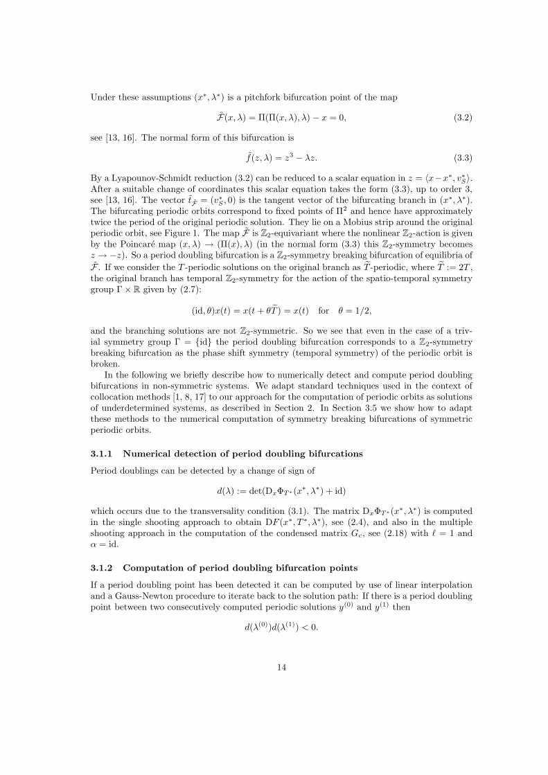
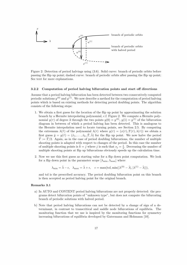
If there is a period halving point y∗ = (x∗, T ∗, λ∗) between two consecutively computedperiodic solutions y(0) and y(1) the vector u goes through zero. As we saw before, a flip bifurcationcorresponds to a pitchfork bifurcation of (3.2). Figure 2 shows the normal form (3.3) of thepitchfork bifurcation and points x(0) and x(1) corresponding to periodic orbits before and afterpassing the bifurcation. For each parameter value λ, the corresponding point on the solid anddashed curve belong to the same periodic orbit, and are conjugate points with respect to theZ2-symmetry action which, for (3.2), is given by x → Π(x, λ), see above. For the points x(0) andx(1) we denote the difference vectors by u(ν) = Π(x(ν), λ(ν))−x(ν), ν = 0, 1. From Figure 2 we seethat the vectors u(0) and u(1) are approximately parallel with opposite sign. At the numericallycomputed solutions y(0) and y(1) the vectors u(y(0)) and u(y(1)) are good approximations foru(0) and u(1). Therefore a period halving point can be detected by the following condition onthe angle between u(y(0)) and u(y(1)):

〈u(y(0)), u(y(1))〉

‖u(y(0))‖‖u(y(1))‖< 0. (3.6)

16

λ

x

branch of periodic orbits

branch of periodic orbits

with halved periodu

(0)

x(0)

u(1)

x(1)

Figure 2: Detection of period halvings using (3.6). Solid curve: branch of periodic orbits beforepassing the flip up point; dashed curve: branch of periodic orbits after passing the flip up point;See text for more explanations.

3.2.2 Computation of period halving bifurcation points and start off directions

Assume that a period halving bifurcation has been detected between two consecutively computedperiodic solutions y(0) and y(1). We now describe a method for the computation of period halvingpoints which is based on existing methods for detecting period doubling points. The algorithmconsists of the following steps:

1. We obtain a first guess for the location of the flip up point by approximating the solutionbranch by a Hermite interpolating polynomial, c.f. Figure 2. We compute a Hermite poly-nomial y(τ) of degree 3 through the two points y(0) = y(0), y(1) = y(1) of the bifurcationdiagram in between of which a period halving has been detected. This is analogous tothe Hermite interpolation used to locate turning points, see Section 2.5. By computingthe extremum λ(τ ) of the polynomial λ(τ) where y(τ) = (x(τ), T (τ), λ(τ)) we obtain a

first guess y = y(τ ) = (x1, . . . , xk , T , λ) for the flip up point. We now halve the periodT := T /2. Again, as in the case of period doubling bifurcations, the number of multipleshooting points is adapted with respect to changes of the period. In this case the numberof multiple shooting points is k = j where j is such that sj = 1

2 . Decreasing the number ofmultiple shooting points at flip up bifurcations obviously speeds up the calculation time.

2. Now we use this first guess as starting value for a flip down point computation. We lookfor a flip down point in the parameter scope [λmin, λmax] where

λmin = λ − ε, λmax = λ + ε, ε = max(tol, min(|λ(0) − λ|, |λ(1) − λ|)),

and tol is the prescribed accuracy. The period doubling bifurcation point on this branchis then accepted as period halving point for the original branch.

Remarks 3.1

a) In AUTO and CONTENT period halving bifurcations are not properly detected: the pro-grams detect bifurcation points of ”unknown type”, but does not compute the bifurcatingbranch of periodic solutions with halved period.

b) Note that period halving bifurcations can not be detected by a change of sign of a de-terminant, in contrast to transcritical and saddle node bifurcations of equilibria. Themonitoring function that we use is inspired by the monitoring functions for symmetryincreasing bifurcations of equilibria developed by Gatermann and Hohmann [10].

17

c) In the computation of bifurcations of equilibria numerical methods based on extendedsystems are frequently employed (see e.g. [1, 16]). One could of course also use such amethod to locate period halving bifurcations. A period halving point could for examplebe computed by solving the system

0 = F (x, T, λ, v) :=

ΦT/2(x; λ) − xDxΦT/2(x; λ)v + v‖v‖2 − 1

using a Newton type method. But since this requires the approximation of the secondderivative of the flow map it would be more expensive than the method that we suggest.

3.3 Bifurcations of periodic orbits with Zp-symmetry

In this section we deal with generic symmetry changing but isotropy preserving secondary bi-furcations of symmetric periodic orbits. The right hand side f of the ODE (1.1) is assumedto be Γ-equivariant under a finite group Γ ⊂ GL(n), as in Section 2.2. We assume that thespatial symmetry K of the periodic orbit is trivial (or restrict the dynamics to Fix(K)). Thisimplies that the spatio-temporal symmetry of the periodic orbits is cyclic: L ' Z`. We can then,without loss of generality, restrict to the case Γ ' Zp for p a multiple of `, see [18]. We describehow the generic secondary bifurcations of periodic orbits with Zp-symmetry, which have beenclassified by Fiedler [9], can be treated numerically. In this section we only deal with bifurcationsof periodic orbits into other periodic orbits (not Hopf bifurcations along branches of periodicorbits).

So let x∗ lie on a periodic orbit P with period T ∗, trivial isotropy K, spatio-temporalsymmetry L = Z` and drift symmetry α. Define the Poincare section as usual by S = x∗ +span(f(x∗))⊥. To examine bifurcations of symmetric periodic orbits the reduced Poincare map

Πred = αΠ, Π : S → α−1S,

from (2.10) is used where Π maps points of S into the points where the positive semi-flow throughx first hits α−1 S. In the case of trivial isotropy K the relationship between the full Poincaremap Π and the reduced Poincare map Πred is given by

Π = α−`Π`red = Π`

red. (3.7)

Here we used that α` = id. Generic bifurcations of symmetric periodic orbits are bifurcations ofthe reduced Poincare map Πred which arise from an eigenvalue ±1 of the Jacobian DxΠred, see[9, 18].

Generic bifurcations of Πred without breaking of the spatial symmetry are turning pointsand period doublings/halvings (flip down and flip up bifurcations); turning points of Πred leadto turning points of the full Poincare map Π. They can be detected and computed in the sameway as in the case of no symmetry, see Section 2.5.

Flip down bifurcations of the reduced Poincare map Πred lead to pitchfork bifurcations re-spectively period doubling bifurcations of Π depending on whether ` is odd or even, see [9]. If` is odd, in particular if the symmetry is trivial (i.e. ` = 1), we have a flip doubling (perioddoubling) bifurcation. If ` is even then a flip pitchfork bifurcation takes place where the periodis preserved, but the spatio-temporal symmetry halved.

3.3.1 Flip pitchfork bifurcation

First we consider the flip pitchfork bifurcation. Let ` be even. Assume that the reduced Poincaremap Πred undergoes a flip down bifurcation. Then the bifurcating solutions x(s), s ∈ R, x(0) =

18

x∗, are fixed points of Π2red. By (3.7),

Π(x(s)) =(Π2

red

)`/2(x(s)) = x(s),

and so the Poincare map Π undergoes a pitchfork bifurcation. Hence the branching solutionshave approximately the same period but their spatio-temporal symmetry L = Z`/2, ˜= `/2 hasbeen halved. The drift symmetry of the bifurcating periodic orbits is α = α2.

3.3.2 Flip doubling bifurcation

Next we consider the flip doubling bifurcation, ie, let ` be odd. Since Π2red(x(s)) = x(s) and ` is

odd the following can be concluded:

Π2(x(s)) = Π2`red(x(s)) = x(s) and Π(x(s)) = Π`

red(x(s)) = Πred(x(s)) 6= x(s).

So the Poincare map Π undergoes a period doubling bifurcation without breaking the symmetryZ`: the spatio-temporal symmetry group of the bifurcating branch is L = Z˜ where ˜ = ` andis generated by the order ` element α = α. Note that the flip doubling bifurcation reduces tothe period doubling bifurcation of non-symmetric systems, see Section 3.1, with ` = 1, α = idwhereas the flip pitchfork bifurcation does not occur for non-symmetric systems.

3.4 Numerical computation of symmetry breaking bifurcations

Since the generic bifurcations of periodic orbits with underlying symmetry group Zp describedabove are generated by periodic doubling bifurcations of the reduced Poincare map they can betreated numerically with the methods for the period doubling bifurcation described in Section3.1.

3.4.1 Detection and computation of flip down bifurcations

Flip down bifurcations are detected by the a sign change of

d(λ) = det(αDxΦT∗

`(x∗) + id), where αDxΦT∗

`(x∗) = Gc,

analogously to the case of no symmetry, see Section 3.1.1. Once a flip down bifurcation has beendetected it can be computed analogously as in the case of non-symmetric systems, see Section3.1.2.

3.4.2 Initialization of the bifurcating branch

Once a flip down point (x∗, T ∗, λ∗) on the original branch has been found, the starting pointy = (x, T , λ) for the bifurcating branch has to be computed. We set T = T ∗ for a flip pitchforkbifurcation and T = 2T ∗ otherwise, and λ = λ∗. Since the number of multiple shooting points isdoubled the second half of x = (x1, . . . , x2k) will be computed by applying the symmetry matrixto the first points:

xi = x∗i for i = 1, . . . , k,

xi+k = α−1x∗i for i = 1, . . . , k.

The tangent vector t = (tx, 0, 0) of the bifurcating branch is computed in a similar way: Thefirst nk components (t1, . . . , tk) of the x-component tx of the tangent t of the bifurcating branchare computed as in Section 3.1.3, with DxΦT∗(x∗) replaced by αDxΦT∗

`(x∗). Then the second

half of tx = (t1, . . . , t2k) is computed by applying the symmetry matrix to the first half andmultiplying it with −1:

ti+k = −α−1ti for i = 1, . . . , k. (3.8)

19

3.5 Numerical computation of symmetry increasing bifurcations

In this section we extend the algorithms for the detection and computation of period halvingpoints for non-symmetric systems (Section 3.2) to systems with symmetry. The main issue hereis the identification of the possible spatio-temporal symmetries of the bifurcating solutions whichare needed for both, the detection of bifurcations and the computation of the bifurcating branch.

3.5.1 Detection of flip up bifurcations

Similarly as in the non-symmetric case, see Section 3.2, flip up points on a branch of periodicorbits with spatio-temporal symmetry L = Z`, trivial isotropy and drift symmetry α are detectedby the angle condition (3.6)

〈u(y(0)), u(y(1))〉

‖u(y(1))‖‖u(y(1))‖< 0

where y(0) and y(1) are two consecutive points on a branch of periodic solutions and

u(x) := αΦ T2`

(x1, λ) − x1 = αxj − x1.

Here the multiple shooting node sj is set to sj = 12 and α is a group element α which satisfies

α2 = α. (3.9)

We now need to classify the possible choices of α and decide whether a flip up doubling or a flipup pitchfork bifurcation occurs.

Theorem 3.2 Let i be such that α = γip where γp generates the symmetry group Γ = Zp of

(1.1). Similarly, write α = γ ip. Then we have:

a) Either i = i2 or i = i+p

2 . Both these values for i are possible if p and i are even, i = i2 is

a possible solution for p odd, i even, and i = i+p2 for p and i odd.

b) (i) If`i = 0 mod p

then a flip up doubling bifurcation takes place. The order ˜ of the drift symmetry αof the bifurcating branch and its period T in the bifurcation point then satisfy

˜= `, T =T ∗

2,

where T ∗ is the period of the original periodic orbit at the bifurcation point.

(ii) If`i 6= 0 mod p

then a flip up pitchfork bifurcation takes place. The order ˜ of the drift symmetry αof the bifurcating branch and its period T in the bifurcation point then satisfy

˜= 2`, T = T ∗.

Proof. From (3.9) we get2i = i mod p,

and soi = (i + jp)/2, j ∈ N. (3.10)

20

Possible solutions to (3.10) which are different modulo p are

i = i/2, i = (i + p)/2.

This proves part a) of the theorem. The rest follows from the definitions of flip pitchfork andflip doubling bifurcations, see Sections 3.3.1 and 3.3.2.

Remark 3.3 Consider a periodic orbit with trivial spatio-temporal symmetry, i.e., α = id,i = 0. Then, if the order p of the symmetry group Γ = Zp is odd and the Γ-action is free, everyflip up bifurcation is a period halving bifurcation. If p is even then a flip up bifurcation of Πred

can be a period halving bifurcation or a flip up pitchfork bifurcation with α = γp2p .

3.5.2 Computation of flip up points and start off tangents

Once the spatio-temporal symmetry of the bifurcating periodic orbit is identified the flip uppoint and the start off directions for the bifurcating branch can be computed in the same wayas for non-symmetric systems, see Section 3.2.

4 Computation of equivariant Hopf points

In this section we show how equivariant Hopf points along branches of periodic orbits can bedetected and computed. For sake of simplicity, we first consider the case of a trivial symmetrygroup Γ = {id}.

4.1 Hopf bifurcations for non-symmetric systems

x2

x1

λ

x∗

f (0)

t(1)f (1)

x(1)

f (0) = f(x(0))

f (1) = f(x(1))

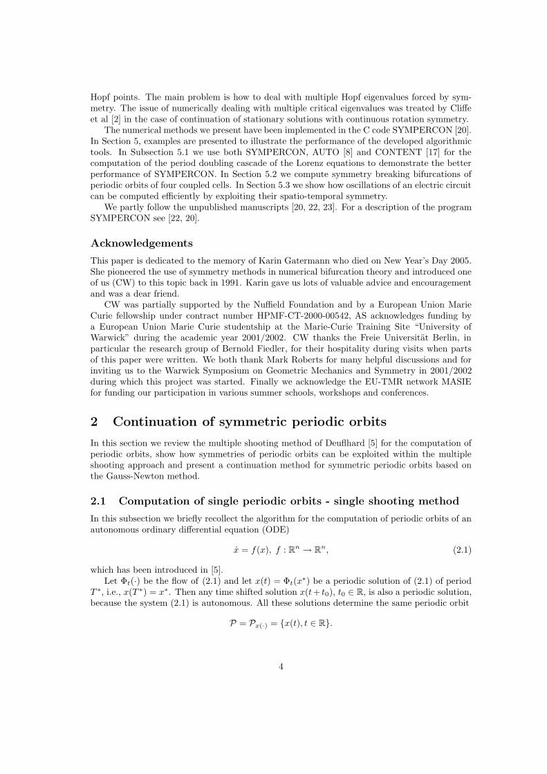
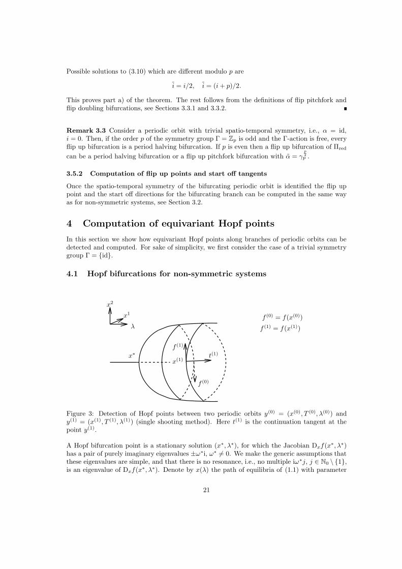
Figure 3: Detection of Hopf points between two periodic orbits y(0) = (x(0), T (0), λ(0)) andy(1) = (x(1), T (1), λ(1)) (single shooting method). Here t(1) is the continuation tangent at thepoint y(1).

A Hopf bifurcation point is a stationary solution (x∗, λ∗), for which the Jacobian Dxf(x∗, λ∗)has a pair of purely imaginary eigenvalues ±ω∗i, ω∗ 6= 0. We make the generic assumptions thatthese eigenvalues are simple, and that there is no resonance, i.e., no multiple iω∗j, j ∈ N0 \ {1},is an eigenvalue of Dxf(x∗, λ∗). Denote by x(λ) the path of equilibria of (1.1) with parameter

21

λ, so that in particular x(λ∗) = x∗. Let µ(λ) be the path of eigenvalues of Dxf(x(λ), λ) suchthat µ(λ∗) = iω∗ and assume that the generic transversality condition

Re

(∂µ

∂λ(λ∗)

)6= 0 (4.1)

is satisfied. Then (see e.g. [13, 16]) a unique branch x(t; ε) of periodic solutions emanates fromthe stationary solution with small amplitude O(ε) and period T (ε) ≈ T (0) = 2π/ω∗. Thissurface of periodic solutions is tangential to the real eigenspace Nω∗ of ±ω∗i, ie Dεx(t; 0) ∈ Nω∗ ,and generically agrees (after a smooth coordinate change) to second order with a paraboloidλ−λ∗ = C(z2

1 +z22), see e.g. [13, 16]. We can consider the Hopf point (x∗, λ∗) as an S1-invariant

2π/ω∗-periodic solution with respect to the action (2.7) of the temporal symmetry group on theperiodic solutions x(t) of (1.1):

x∗(t) ≡ x∗ ∀ t =⇒ (id, θ) x∗(t) = x∗(t) ∀ t.

Hence the Hopf bifurcation is an S1-symmetry breaking bifurcation.

4.1.1 Detection of Hopf points along branches of periodic orbits

If a pathfollowing algorithm for periodic solutions runs through a Hopf point the continuationdirection changes its sign and the same path of periodic orbits is computed again. ThereforeHopf points which occur during the pathfollowing of periodic orbits should be detected so thatthe pathfollowing routine can be stopped at the Hopf point. If there is a Hopf point between twoconsecutively computed periodic orbits y(0) and y(1), where y = (x, T, λ), x = (x1, . . . , xk), thenthe vectors f(xi), which are the infinitesimal generators of the S1-symmetry in the point xi, gothrough zero. Thus f(xi) is a symmetry monitoring function in this case. If the angle betweenthe vectors f(xi) of two consecutively computed periodic orbits is greater than 90 degree, i.e.,if for some i ∈ {1, . . . , k},

〈f(x(0)i ), f(x

(1)i )〉

‖f(x(0)i )‖‖f(x

(1)i )‖

< 0

then there is a Hopf point on the branch of periodic orbits between the y(0) and y(1), c.f. Figure3.

Remark 4.1 Note that in the program packages AUTO [8] and CONTENT [17] the numericalpart of which is based on AUTO Hopf points along periodic orbits are not detected properly.They are detected as general cycle branching points, but when switching to the bifurcatingbranch of stationary solutions an error occurs.

4.1.2 Computation of Hopf bifurcations of non-symmetric systems

If a Hopf point along a path of periodic orbits is detected, it can be computed by an extendedsystem [12, 14], see also the review in [1]. We use a slightly different form of extended systemwhich is underdetermined and does not fix the phase of the Hopf eigenvector to be computed.We present this extended system briefly in this subsection.

Let x∗ be Hopf point, i.e., an equilibrium f(x∗, λ∗) = 0, the Jacobian Dxf(x∗, λ∗) of whichhas a pair of purely imaginary eigenvalues ±iω∗. Hence

Dxf(x∗, λ∗)(v∗ + iw∗) = iω∗(v∗ + iw∗).

So we get

Dxf(x∗, λ∗)v∗ = −ω∗w∗, Dxf(x∗, λ∗)w∗ = ω∗v∗, ‖w∗‖2 + ‖v∗‖2 = 1.

22

Define F : R3n+2 → R3n+1 where

F (x, λ, v, w, ω) =

f(x, λ)Dxf(x, λ)v + ωwDxf(x, λ)w − ωv〈v, v〉 + 〈w, w〉 − 1

. (4.2)

Then F = 0 yields the Hopf point and its imaginary eigenvalue and corresponding eigenvector.Moreover we have:

Theorem 4.2 If the eigenvalue ±iω∗ is simple, if Dxf(x∗, λ∗) is invertible and if the transver-sality condition (4.1) holds, then the Gauss-Newton method applied to (4.2) converges for suffi-ciently good initial data.

The proof of this theorem is basically contained in [1, 12, 14]. As shown there the transversalitycondition Re µ′(λ∗) 6= 0 implies that any kernel vector t = (tx, tλ, tv , tw, tω) of the derivativeDF (x∗, λ∗, v∗, w∗, ω∗) of F in the Hopf point satisfies tω = 0, tλ = 0 and tx = 0 and hence(tv , tw) satisfies the equations

0 = Dxf(x∗, λ∗)tv + ω∗tw (4.3)

0 = Dxf(x∗, λ∗)tw − ω∗tv (4.4)

0 = 2〈v∗, tv〉 + 2〈w∗, tw〉. (4.5)

Therefore tv + itw is a Hopf eigenvector. Equation (4.5) and the fact that the Hopf eigenvalueiω∗ is a simple eigenvalue of Dxf(x∗, λ∗) imply that the kernel of DF in the Hopf point is one-dimensional. Hence DF has full rank in the Hopf point and the Gauss-Newton method appliedto (4.2) converges for sufficiently good initial data. As we will see later (see Sections 4.2.1 and5.2), symmetry often inforces multiple Hopf eigenvalues, so that the extended system (4.2) hasto be modified in the case of equivariant Hopf points.

Initial guess for the Gauss-Newton iteration An initial guess for a Hopf point detectedbetween two periodic orbits y(0) = (x(0), T (0), λ(0)) and y(1) = (x(1), T (1), λ(1)), where x =(x1, . . . , xk), can be obtained by Hermite interpolation y(τ) between those points over the liney(0) + τ(y(1) − y(0)), τ ∈ [0, 1], such that y(0) = y(0), y(1) = y(1), and by computing the pointy = y(τ ) = (x(τ ), T (τ), λ(τ )) such that λ′(τ ) = 0, analogously to the computation of initialguesses for a turning point, see Section 2.5. We then set

x := x1(τ ),

define an approximation for the Hopf frequency ω as

ω =2π

T, where T = T (τ),

and an approximation for the parameter value of the Hopf point as

λ = λ(τ ).

We moreover define initial guesses v + iw for the Hopf eigenvector as

v = cd

dτx1(τ ), w = −

1

ωDxf(x, λ)v

with c such that‖v‖2 + ‖w‖2 = 1.

The point (x, λ, v, w, ω) is then used as initial guess for the Newton iteration applied to (4.2).

23

4.2 Detection and computation of equivariant Hopf points

In this section we extend the methods for the computation of Hopf points of non-symmetricsystems from Section 4.1 to systems with symmetry. The main issue here is how to deal withmultiple Hopf eigenvalues forced by symmetry which lead to convergence failure of the extendedsystem (4.2) for the computation of Hopf points of non-symmetric systems.

4.2.1 Equivariant Hopf points

We are starting from a Γ-invariant stationary solution (x∗, λ∗), i.e., Γx∗ = Γ. We assume thatthe Jacobian Dxf(x∗, λ∗) has a pair ±ω∗i of purely imaginary eigenvalues, ω∗ 6= 0, and thatthere are no resonances, i.e., ±jiω∗, j = 0, 2, 3, 4, . . ., is not an eigenvalue of Dxf(∗, λ∗). Asbefore let Nω∗ be the real eigenspace of Dxf(x∗, λ∗).

Lemma 4.3 [11] If γ ∈ Γx then γDxf(x, λ) = Dxf(x, λ)γ. Moreover, every eigenspace ofDxf(x, λ) is Γx-invariant.

Proof. The first statement follows from the Γ-equivariance of f and the γ-invariance of x. Forthe second statement let u be a complex eigenvector of A = Dxf(x, λ) to the eigenvalue µ. SinceγA = Aγ we have Aγu = γAu = γµu so that γu is an eigenvector of A to the eigenvalue µ aswell.

As a consequence, Dxf(x∗, λ∗) is Γ-equivariant and Nω∗ is Γ-invariant. Hence Nω∗ can bedecomposed into irreducible Γ-invariant subspaces, see Remark 2.4.

Definition 4.4 [11] We call an eigenvalue µ of a Γ-equivariant matrix A a Γ-simple eigenvalueof A if the real eigenspace N of A to the eigenvalue µ is irreducible.

We make the generic assumption that iω∗ is a Γ-simple eigenvalue of Dxf(x∗, λ∗). This meansthat iω∗ has the lowest multiplicity allowed by the symmetry group Γ.

Since Dxf(x∗, λ∗) is invertible, by the implicit function theorem applied to Fix(Γ) = Rnred

there is a path x(λ) of Γ-invariant equilibria of (1.1) with x(λ∗) = x∗. As in the case of thestandard Hopf bifurcation we assume that the transversality condition (4.1) holds for the pathµ(λ) of the pair of eigenvalues of Dxf(x(λ), λ) with µ(λ∗) = iω∗.

We define the operation of Γ × S1 on a T -periodic solution x(t) as in (2.7)

(γ, θ)x(t) = γx(t + θ T ) for (γ, θ) ∈ Γ × S1,

and the operation of Γ × S1 on the real eigenspace Nω∗ of ±ω∗i of Dxf(x∗, λ∗) by

(γ, θ)u = γeθDxf(x∗,λ∗)T∗

u, (γ, θ) ∈ Γ × S1, u ∈ Nω∗ , (4.6)

where T ∗ = 2πω∗

.

Theorem 4.5 [11] (Equivariant Hopf Theorem) Let the above conditions be satisfied. If thenfor a subgroup L ⊂ Γ × S1 the fixed point space

NLω∗ := {u ∈ Nω∗ : (γ, θ)u = u ∀ (γ, θ) ∈ L} (4.7)

satisfies the conditiondim NL

ω∗ = 2, (4.8)

then there is a unique branch x(t; ε) of periodic solutions with amplitude O(ε) bifurcating from(x∗, λ∗) with Dεx(t; 0) ∈ NL

ω∗, with parameter λ(ε), such that λ(0) = λ∗, with minimal periodsT (ε), such that T (0) = 2π/ω∗, and with L as spatio-temporal symmetry group.

24

As in the non-symmetric case the bifurcating periodic orbits generically lie on a paraboloid, seeFigure 3.

Remark 4.6 The equivariant Hopf theorem provides the spatio-temporal symmetries L of thebifurcating periodic orbits and the planes NL

ω∗ from which the start off directions for the em-anating periodic orbits can be chosen: We define the phase space for the bifurcating periodicorbit with symmetry L as Fix(K) where K, the group of spatial symmetries of the periodicorbit, is the kernel of the homomorphism Θ of the periodic orbit, see (2.6), and thus

K = {γ ∈ Γ, (γ, 0) ∈ L}.

We compute the integer ` such that L/K ' Z`, see (2.8), and the drift symmetry α of theperiodic orbit by determining the element (α, θ∗) in L with the smallest non-zero phase shiftθ∗ = 1

` , c.f. (2.9). We identify the Hopf point (x∗, λ∗) with a periodic orbit which has periodT ∗ = 2π

ω∗, multiple shooting points x∗

i = x∗ for i = 1, . . . k and the parameter λ∗. Similarly asin the non-symmetric case (c.f. [1]) we then define the continuation tangent t∗ = (t∗x, t∗T , t∗λ) atthis Hopf periodic orbit as follows:

t∗T = 0, t∗λ = 0, t∗x = (t∗1, . . . , t∗k),

wheret∗i = cos(siT

∗/`)v∗ + sin(siT∗/`)w∗, i = 1, . . . , k.

Here v∗ + iw∗ is the eigenvector to the purely imaginary eigenvalue ω∗i of Dxf(x∗, λ∗) which isdetermined by the condition v∗, w∗ ∈ NL

ω∗ . See Sections 5.2 and 5.3 for applications.

4.2.2 Detection of equivariant Hopf points

Equivariant Hopf points along branches of periodic orbits are detected in the same way as Hopfpoints of non-symmetric systems, see Section 4.1.1.

4.2.3 Computation of equivariant Hopf bifurcations

As mentioned in Section 4.1.2 the extended system (4.2) for the computation of Hopf pointsof non-symmetric systems only converges if the Hopf eigenvalue iω∗ is simple. In the caseof symmetric dynamical systems this assumption can only be satisfied if the correspondingirreducible representation is one-dimensional. In general the symmetry might enforce multipleeigenvalues (see Section 5.2 for an example). Therefore the numerical method for computingHopf points from Section 4.1.2 has to be modified in the case of symmetric dynamical systems.In this section we present an efficient algorithm for computing equivariant Hopf points whichapplies to Hopf points which satisfy the conditions of the equivariant Hopf theorem.

Assume that an equivariant Hopf point (x∗, λ∗) with Hopf eigenvalue ±iω∗, ω∗ > 0, has beendetected numerically along a branch of periodic orbits of the Γ-equivariant ODE (1.1) with driftsymmetry α of order ` and, for simplicity, trivial isotropy K (restrict the dynamics to Fix(K)and replace Γ by N(K)/K otherwise). As before we denote by L ' Z` the spatio-temporalsymmetry of the branch of periodic orbits. Then the Hopf point x∗ is L-invariant: L ⊆ Γx∗ . Wemake the assumptions of the equivariant Hopf Theorem 4.5 replacing Γ by Γx∗ and denote theplane tangent to the branch of periodic orbits at the Hopf point by NL

ω∗ , as in (4.7).We will now formulate an algorithm for the computation of the equivariant Hopf point (x∗, λ∗)

along with the Hopf frequency ω∗ and the corresponding Hopf eigenvector v∗ + iw∗ satisfyingv∗, w∗ ∈ NL

ω∗ .

25

Note that the condition of the equivariant Hopf Theorem 4.5 that NLω∗ is 2-dimensional is

equivalent to requiring that there is only one eigenvector v∗+iw∗ of Dxf(x∗, λ∗) to the eigenvalue±iω∗ satisfying

v∗ + iw∗ = αe2π

ω∗`Dxf(x∗,λ∗)(v∗ + iw∗). (4.9)

Solving the nonlinear equation (4.9) numerically using an extended system would involve thecomputation of the exponential exp( 2π

ω`Dxf(x∗, λ∗)) of Dxf(x∗, λ∗) which is in general expensive.An extended system involving Dxf(x∗, λ∗) rather than its exponential, like the system (4.2) inthe case of non-symmetric systems, is therefore preferable. To derive such a system we use thefollowing approach: Note that

Dxf(x∗, λ∗)(v∗ + iw∗) = iω∗(v∗ + iw∗)

and so

exp

(2π

ω∗`Dxf(x∗, λ∗)

)(v∗ + iw∗) = e

2πi` (v∗ + iw∗)

and henceα(v∗ + iw∗) = e−

2πi` (v∗ + iw∗). (4.10)

So v∗ +iw∗ lies in the the complex eigenspace of α to the eigenvalue e−2πi/` which we denote byXc

` ⊂ Xc = Cn, and v∗ and w∗ lie in the real eigenspace of α to the eigenvalue e−2πi/` which wedenote by X`. So X` is the L-invariant subspace of X = Rn where α, the generator of L ' Z`,acts as a rotation by −2π/`.

The following lemma is crucial for the numerical computation of equivariant Hopf points.

Lemma 4.7 Let the assumptions of the equivariant Hopf theorem 4.5 hold. If then v +iw ∈ X c`

is an eigenvector of Dxf(x∗, λ∗) to the eigenvalue iω∗ then v + iw = c(v∗ + iw∗) for some c ∈ C

where v∗ + iw∗ is a Hopf eigenvector with v∗, w∗ ∈ NLω∗ .

Proof. The vector v +iw satisfies (4.9) and by the assumption of the equivariant Hopf theorem4.5 there is only one such eigenvector (over C), namely v∗ + iw∗. This proves the lemma.

Due to this lemma, we can solve (4.9) as follows: We first compute the space X `c . Then we

compute the L-invariant Hopf point together with a Hopf eigenvector which lies in X` by anextended system.

First step of the algorithm. We compute an orthonormal basis of X c` and store it as row

vectors of a matrix E`. We assume that ` > 1, i.e., that the branch of periodic orbits alongwhich a Hopf bifurcation has been detected has non-trivial spatio-temporal symmetry L = Z`.We consider two cases:

Case 1: ` = 2. We compute the kernel X2 = ker(B2) of B2 = α + idn and store an orthonormalbasis of it in the row vectors of the (d, n)-matrix E2. Here d = dim X2 and X2 is the L-invariantsubspace of Rn where the action of the symmetry group L = Z2 generated by α is given byα|X2 = −1. Hence,

ET2 E2 = id |X2 . (4.11)

Case 2: ` > 2. In this case we compute the null space of the (2n, 2n)-matrix

B` :=

(α − cos(2π/`) idn − sin(2π/`) idn

sin(2π/`) idn α − cos(2π/`) idn

). (4.12)

We store an orthonormal basis of ker(B`) in the row vectors of the matrix E` = [EV , EW ] ∈Mat(d, 2n) where EV , EW ∈ Mat(d, n).

Before we continue with the description of the algorithm we present the following lemma:

26

Lemma 4.8 Let ` > 2. Then the following holds true:

a) If (v, w) ∈ kerB`, v, w ∈ Rn, we have v + iw ∈ Xc` .

b) If (v, w) ∈ kerB`, then so is (−w, v). In particular, kerB` has even dimension d = 2d,

d ∈ N, the eigenvalue e−2πi/` of α has geometric multiplicity d , and d = dim X`.

c) For any x ∈ Rd we have ETV x + iET

W x ∈ Xc` .

d) Both ETV and ET

W have X` as range.

Proof.

a) By Definition, v +iw ∈ Xc` if and only if v +iw satisfies (4.10). Taking real and imaginary

parts of the left and right hand side of (4.10) we see that v + iw satisfies (4.10) iff (v, w) ∈kerB`.

b) follows from a) and the fact that (v, w) ' v + iw and i(v + iw) ∼ (−w, v) are linearlyindependent over R.

c) follows from the definition of E`.

d) follows from a) and b).

Second step of the algorithm. Again we consider two cases: ` = 2, ` > 2.

Case 1: ` = 2. We solve an extended system

F (xred, λ, vred, wred, ω) = 0,

similarly to (4.2), where now

vred, wred ∈ X` ' Rd, xred ∈ Fix(L) ' R

nred

andF : R

nred+2d+2 → Rnred+2d+1.

Let fred := f |Fix(L) and let Q : Rn → Rnred be the matrix which contains an orthonormal basisof Fix(L), dim Fix(L) = nred, as row vectors. Then we define F as

F (xred, λ, vred, wred, ω) =

fred(xred, λ)E2Dxf(x, λ)|x=QT xred

ET2 vred + ωwred

−ωvred + E2Dxf(x, λ)|x=QT xredET

2 wred

〈vred, vred〉 + 〈wred, wred〉 − 1

. (4.13)

Case 2: ` > 2. In this case the real part v∗ of the Hopf eigenvector v∗ + iw∗ and the knowledgeof the drift symmetry α of the branch of periodic orbits along which a Hopf bifurcation wasdetected determines the Hopf eigenvector uniquely since v∗ + iw∗ satisfies (4.10) and so

w∗ =1

sin(2π/`)(αv∗ − cos(2π/`)v∗) .

27

Therefore only the real part of the Hopf eigenvector, the Hopf point, its parameter and the Hopffrequency need to be computed by an extended system. We define F : Rnred+d+2 → Rnred+d+1

by

F (xred, λ, vred, ω) =

fred(xred, λ)EV (Dxf(x, λ)|x=QT xred

ETV vred + ωET

W vred)〈vred, vred〉 − 1

. (4.14)

Proposition 4.9

a) If ` = 2 and (x∗red, λ∗, v∗red, w∗

red, ω∗) is a solution to F = 0 as defined in (4.13) then

x∗ = QT x∗red is an equivariant Hopf point with Hopf frequency ω∗. Moreover a Hopf

eigenvector v∗ + iw∗ with v∗, w∗ ∈ NLω∗ is given by v∗ = ET

2 v∗red, w∗ = ET2 w∗

red.

b) Similarly, if ` > 2, and (x∗red, λ∗, v∗red, ω

∗) is a solution to F = 0 as defined in (4.14)then x∗ = QT x∗

red is an equivariant Hopf point with Hopf frequency ω∗. Moreover a Hopfeigenvector v∗ + iw∗ with v∗, w∗ ∈ NL

ω∗ is given by v∗ = ETV v∗red, w∗ = ET

W v∗red.

For the proof we need the following lemma:

Lemma 4.10 Let A be an (n, n)-matrix which is equivariant with respect to a linear Z`-actionon Rn. Let α generate Z` and define X` as before. Then X` is A-invariant.

Proof. Let v ∈ X`. Then there is some w ∈ X` such that v + iw is an eigenvector of α to theeigenvalue exp(−2πi/`). By Z`-equivariance of A also A(v + iw) is an eigenvector of α to theeigenvalue exp(−2πi/`) and so both Av and Aw lie in X`.

Note that X` is an isotypic component of the Z` action on Rn, and that generally isotypic com-ponents for a linear action of a group Γ are invariant under Γ-equivariant matrices [11].

Proof of Proposition 4.9.

a) Case ` = 2. The first equation fred(x, λ) = 0 of F = 0 implies that x∗red is an equilibrium

of fred(·, λ∗). Hence x∗ = QT x∗

red is an L-invariant equilibrium of f(·, λ∗). From the otherequations in F = 0 we conclude that v∗

red + iw∗red is an eigenvector of E2Dxf(x∗, λ∗)ET

2

to the eigenvalue iω∗. Since x∗ ∈ Fix(L) the derivative Dxf(x∗, λ∗) is L-equivariantby Lemma 4.3 and therefore, by Lemma 4.10, maps X2 into itself. Let v∗ = ET

2 v∗red,w∗ = ET

2 w∗red. Because of (4.11), v∗ + iw∗ ∈ Xc

2 is an eigenvector of Dxf(x∗, λ∗) to theeigenvalue iω∗. Hence (x∗ = QT x∗

red, λ∗) is a Hopf point. Lemma 4.7 now implies thatv∗, w∗ ∈ NL

ω∗ .

b) Case ` > 2. As in the case ` = 2 the first equation of F = 0 implies that x∗ = QT x∗red is an

L-invariant equilibrium of f(·, λ∗). Let v∗ = ETV v∗red and w∗ = ET

W w∗red. From Lemma 4.8

c) we conclude that v∗ + iw∗ ∈ Xc` . Since Dxf(QT xred(λ), λ) is L-equivariant by Lemma

4.3 and hence maps X` into itself by Lemma 4.10 and since EV |X`is an isomorphism by

Lemma 4.8 d), the other equations in F = 0 imply that

Dxf(x∗, λ∗)v∗ + ω∗w∗ = 0 (4.15)

and soRe(Dxf(x∗, λ∗)(v∗ + iw∗) − iω∗(v∗ + iw∗)) = 0.

Multiplying (4.15) by α and using the L-equivariance of Dxf(x∗, λ∗) we obtain

Dxf(x∗, λ∗)αv∗ + ω∗αw∗ = 0.

28

From the fact that v∗ + iw∗ ∈ Xc` we conclude

Re(e−2πi/`(Dxf(x∗, λ∗)(v∗ + iw∗) − iω∗(v∗ + iw∗))

)= 0.

Since e2πi/` /∈ R this implies that

Dxf(x∗, λ∗)(v∗ + iw∗) = iω∗(v∗ + iw∗)

and therefore (x∗, λ∗) is a Hopf point and v∗ + iw∗ ∈ Xc` a Hopf eigenvector. By Lemma

4.7 we then get v∗, w∗ ∈ NLω∗ .

Analogously to Theorem 4.2 we have:

Theorem 4.11 If the assumptions of the equivariant Hopf Theorem 4.5 hold and if the initialguess is good enough then the Gauss-Newton method applied to (4.13) for ` = 2 and applied to(4.14) for ` > 2 converges.

Proof. Similarly as in the non-symmetric case (Theorem 4.2, see [1, 12, 14]) we show that DF ,with F from (4.13) for ` = 2 and from (4.14) for ` > 2, has full rank in the Hopf point. Asbefore we consider the cases ` = 2 and ` > 2 separately.

Case ` = 2. The assumptions of the equivariant Hopf theorem imply that iω∗ is a simple eigen-value of Dxf(x∗, λ∗)|X2 and hence, due to (4.11), also of E2Dxf(x∗, λ∗)ET

2 . The proof that DFhas full rank in the Hopf point is therefore very similar to the non-symmetric case: the onlydifference is that we require v, w ∈ X2 and x ∈ Fix(L). We omit the details.

Case ` > 2. In this case we have

D(xred,λ,vred,ω)F (xred, λ, vred, ω) =

Dxredfred(xred, λ) Dλfred(xred, λ) 0 0

EV D2xfET

V vredQT EV DxDλfET

V vred EV (DxfETV + ωET

W ) EV ETW vred

0 0 2vTred 0

,

where f is short for f(QT xred, λ). Let t = (txred, tλ, tvred

, tω) be a kernel vector of DF in theequivariant Hopf point:

0 = Dxredfred(x

∗red, λ∗)txred

+ Dλfred(x∗red, λ∗)tλ,

0 = EV D2xfET

V v∗redQT txred+ EV DxDλfET

V v∗redtλ

+EV (DxfETV + ω∗ET

W )tvred+ EV ET

W v∗redtω ,

0 = 2〈v∗red, tvred

〉.

(4.16)

We need to show that ker(DF ) is one-dimensional. Similarly, as in the proof of convergence forthe non-symmetric case, Theorem 4.2, see e.g. [1, 12, 14], we conclude from the first equation of(4.16) that

(txred, tλ) = tλ(x′

red(λ∗), 1).

Since

D2xf(x∗, λ∗)x′(λ∗) + DxDλf(x∗, λ∗) =

d

dλDxf(x(λ), λ)|λ=λ∗ ,

29

where x(λ) = QT xred(λ), we deduce from the second equation of (4.16) that

EV

(tλ

d

dλDxf(x(λ), λ)|λ=λ∗ET

V v∗red + (Dxf(x∗, λ∗)ETV + ω∗ET

W )tvred+ tωET

W v∗red

)= 0.

(4.17)Since ET

V v∗red, ETV tv, E

TW v∗red, E

TW tv ∈ X` and EV |X`

is an isomorphism by Lemma 4.8 d) andsince Dxf(x(λ), λ) maps X` into itself by Lemmata 4.3 and 4.10, (4.17) implies that

tλd

dλDxf(x(λ), λ)|λ=λ∗ET

V v∗red + Dxf(x∗, λ∗)ETV tv + ω∗ET

W tv + tωETW v∗red = 0.

Let tv = ETV tvred

and tw = ETW tvred

. By Lemma 4.8 c) we have tv +itw ∈ Xc` which we will need

later on. Denote v∗ = ETV v∗red, w∗ = ET

W v∗red such that, by Proposition 4.9 b), v∗ +iw∗ is a Hopfeigenvector. Then we get

0 = tλd

dλDxf(x(λ), λ)|λ=λ∗v∗ + Dxf(x∗, λ∗)tv + ω∗tw + tωw∗

= Re

(tλ

d

dλDxf(x(λ), λ)|λ=λ∗ (v∗ + iw∗) + Dxf(x∗, λ∗)(tv + itw)

)

−Re (iω∗(tv + itw) + itω(v∗ + iw∗)) .

By Lemma 4.8 c), v∗ + iw∗ ∈ Xc` . Therefore

0 = αtλddλ Dxf(x(λ), λ)|λ=λ∗v∗ + αDxf(x∗, λ∗)tv + ω∗αtw + tωαw∗

= tλddλ Dxf(x(λ), λ)|λ=λ∗αv∗ + Dxf(x∗, λ∗)αtv + ω∗αtw + tωαw∗

= Re(e−2πi/`(tλ

ddλ Dxf(x(λ), λ)|λ=λ∗ (v∗ + iw∗) + Dxf(x∗, λ∗)(tv + itw))

)

−Re(e−2πi/`(iω∗(tv + itw) − itω(v∗ + iw∗))

),

where we used the L-equivariance of Dxf(x(λ), λ) (Lemma 4.3) in the second line. Since e−2πi/` /∈R for ` > 2 these last two equations imply that

0 = tλddλ Dxf(x(λ), λ)|λ=λ∗ (v∗ + iw∗)

+Dxf(x∗, λ∗)(tv + itw) − iω∗(tv + itw) − itω(v∗ + iw∗).(4.18)

Let v(λ) + iw(λ), v(λ∗) = v∗, w(λ∗) = w∗, v(λ), w(λ) ∈ X`, be the path of eigenvectors ofDxf(x(λ), λ) to the eigenvalues µ(λ) with ‖v(λ)‖ = 1. Let u∗ = v∗ + iw∗ and let u∗

L ∈ Xc` be

the uniquely determined left eigenvector of Dxf(x∗, λ∗) to the eigenvalue iω∗ with 〈u∗L, u∗〉 = 1.

As in the non-symmetric case, see [1, 14, 12], (4.18) then implies that

tλu∗L

d

dλDxf(x(λ), λ)λ=λ∗u∗ = itω .

This combined with

〈u∗L,

d

dλDxf(x(λ), λ)λ=λ∗u∗〉 = µ′(λ∗)

and the assumption that Re µ′(λ∗) 6= 0 gives tλ = 0. Hence tx = 0 and tω = 0. As in the proofof Theorem 4.2, (4.18) reduces to

Dxf(x∗, λ∗)(tv + itw) − iω∗(tv + itw) = 0

30

so that tv + itw is a Hopf eigenvector. Since tv + itw ∈ Xc` we deduce from Lemma 4.7 that

tv + itw = c(v∗ + iw∗) for some c ∈ C. By the definition of v∗, w∗ and tv, tw this is equivalent to

ETV tvred

+ iETW tvred

= c(ETV v∗red + iET

W v∗red). (4.19)

By Lemma 4.8 the map EV ETV ∈ Mat(d) is invertible. Therefore we conclude from (4.19) that

tvred∈ span(v∗red, w∗

red), where w∗red := (EV ET

V )−1EV ETW v∗red. From the last row of DF we get

the additional condition 〈v∗red, tvred

〉 = 0 on tvred. Hence the kernel of DF is one-dimensional and

DF has full rank in the Hopf point.

Initial guess for the Gauss-Newton iteration As in the non-symmetric case, see Section4.1.2, we use Hermite interpolation between two consecutive periodic orbits y(0) and y(1) be-tween of which a Hopf bifurcation was detected and determine the point τ on the interpolatingpolynomial y(τ) = (x(τ), T (τ), λ(τ)) with λ′(τ ) = 0. This way we obtain an initial approxima-

tion x = x(τ ) for the Hopf point, an initial approximation λ = λ(τ ) for its parameter, and aninitial approximation ω = 2π

Tfor its frequency, where T = T (τ). If ` = 2 we let

v = c E2d

dτx1(τ ), w = −c

1

ωDxf(x, λ)

d

dτx1(τ )

where c is such that 〈v, v〉+ 〈w, w〉 = 1 and take the point (xred = Qx, λ, v, w, ω) as initial guessfor the Gauss-Newton iteration applied to (4.13). If ` > 2 we define

v = cEVd

dτx1(τ )

with c ∈ R such that 〈v, v〉 = 1 and use (xred, λ, v, ω) as initial guess for the Gauss-Newtoniteration applied to (4.14).

5 Applications

In this section we illustrate the numerical methods for the continuation of symmetric periodicorbits which we presented in the preceding sections and implemented in the code SYMPERCON[20] with some examples.

5.1 The Lorenz model - comparison with AUTO and CONTENT

There are many programs for the numerical continuation of periodic orbits of non-symmetricsystems. Two of the most well known and widely used programs are AUTO [8] and CONTENT[17] the numerical part of which is based on AUTO. In both programs collocation is used tofind periodic solutions. This approach is equivalent to the multiple shooting ansatz with themultiple shooting points being the grid points and the IVP solver having only one step.

One of the key new features of SYMPERCON compared to those program packages is theexploitation of symmetries of periodic orbits and the computation of symmetry breaking andsymmetry increasing bifurcations, and we present some applications of these methods in the nextsections. In this section we give numerical evidence that the program package SYMPERCONis also competitive when applied to continuation of non-symmetric periodic orbits. We comparethe programs AUTO, CONTENT and SYMPERCON using an example which is taken from

31

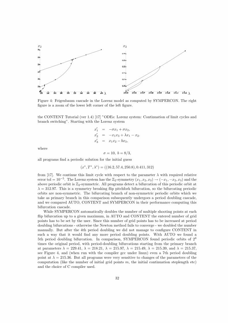
λ

x2

λ

x2

Figure 4: Feigenbaum cascade in the Lorenz model as computed by SYMPERCON. The rightfigure is a zoom of the lower left corner of the left figure.

the CONTENT Tutorial (ver 1.4) [17] ”ODEs: Lorenz system: Continuation of limit cycles andbranch switching”. Starting with the Lorenz system

x′1 = −σx1 + σx2,

x′2 = −x1x3 + λx1 − x2.

x′3 = x1x2 − bx3,

whereσ = 10, b = 8/3,

all programs find a periodic solution for the initial guess

(x∗, T ∗, λ∗) = ((16.2, 57.4, 250.8), 0.411, 312)

from [17]. We continue this limit cycle with respect to the parameter λ with required relativeerror tol = 10−5. The Lorenz system has the Z2-symmetry (x1, x2, x3) → (−x1,−x2, x3) and theabove periodic orbit is Z2-symmetric. All programs detect a bifurcation of this periodic orbit atλ = 312.97. This is a symmetry breaking flip pitchfork bifurcation, so the bifurcating periodicorbits are non-symmetric. The bifurcating branch of non-symmetric periodic orbits which wetake as primary branch in this comparison subsequently undergoes a period doubling cascade,and we compared AUTO, CONTENT and SYMPERCON in their performance computing thisbifurcation cascade.

While SYMPERCON automatically doubles the number of multiple shooting points at eachflip bifurcation up to a given maximum, in AUTO and CONTENT the entered number of gridpoints has to be set by the user. Since this number of grid points has to be increased at perioddoubling bifurcations - otherwise the Newton method fails to converge - we doubled the numbermanually. But after the 4th period doubling we did not manage to configure CONTENT insuch a way that it would find any more period doubling points. With AUTO we found a5th period doubling bifurcation. In comparison, SYMPERCON found periodic orbits of 26

times the original period, with period-doubling bifurcations starting from the primary branchat parameters λ = 229.41, λ = 218.21, λ = 215.97, λ = 215.49, λ = 215.39, and λ = 215.37,see Figure 4, and (when run with the compiler gcc under linux) even a 7th period doublingpoint at λ = 215.36. But all programs were very sensitive to changes of the parameters of thecomputation (like the number of initial grid points m, the initial continuation steplength etc)and the choice of C compiler used.

32

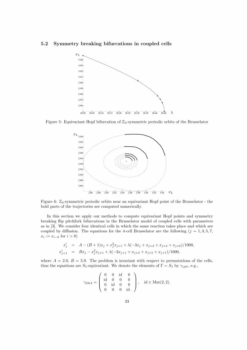
5.2 Symmetry breaking bifurcations in coupled cells

++

+

+

+

+

20.00 20.05 20.10 20.15 20.20 20.25 20.30 20.35 20.40 20.45

2.96

2.97

2.98

2.99

3.00

3.01

3.02

3.03

3.04

+ + + + + + + + + +

+

+

+

+

+

+

+

+

+

x4

λ

Figure 5: Equivariant Hopf bifurcation of Z4-symmetric periodic orbits of the Brusselator

++

+

+

+

+

2.86 2.88 2.90 2.92 2.94 2.96 2.98 3.00 3.02 3.04

2.86

2.88

2.90

2.92

2.94

2.96

2.98

3.00

3.02

3.04

+ + + + + + + + + +

+

+

+

+

+

+

+

+

+

+x4

x2

Figure 6: Z4-symmetric periodic orbits near an equivariant Hopf point of the Brusselator - thebold parts of the trajectories are computed numerically.

In this section we apply our methods to compute equivariant Hopf points and symmetrybreaking flip pitchfork bifurcations in the Brusselator model of coupled cells with parametersas in [3]. We consider four identical cells in which the same reaction takes place and which arecoupled by diffusion. The equations for the 4-cell Brusselator are the following (j = 1, 3, 5, 7,xi := xi−8 for i > 8)

x′j = A − (B + 1)xj + x2

jxj+1 + λ(−3xj + xj+2 + xj+4 + xj+6)/1000,

x′j+1 = Bxj − x2

jxj+1 + λ(−3xj+1 + xj+3 + xj+5 + xj+7)/1000,

where A = 2.0, B = 5.9. The problem is invariant with respect to permutations of the cells,thus the equations are S4-equivariant. We denote the elements of Γ = S4 by γijkl , e.g.,

γ2314 =

0 0 id 0id 0 0 00 id 0 00 0 0 id .

, id ∈ Mat(2, 2).

33

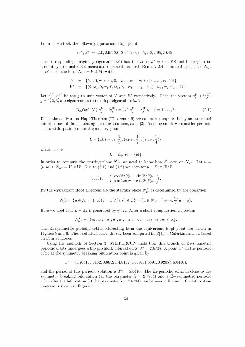
From [3] we took the following equivariant Hopf point

(x∗, λ∗) = (2.0, 2.95, 2.0, 2.95, 2.0, 2.95, 2.0, 2.95, 20.45).

The corresponding imaginary eigenvalue ω∗i has the value ω∗ = 0.62058 and belongs to anabsolutely irreducible 3-dimensional representation, c.f. Remark 2.4. The real eigenspace Nω∗

of ω∗i is of the form Nω∗ = V ⊕ W with

V = {(v1, 0, v2, 0, v3, 0,−v1 − v2 − v3, 0) | v1, v2, v3 ∈ R},

W = {(0, w1, 0, w2, 0, w3, 0,−w1 − w2 − w3) | w1, w2, w3 ∈ R}.

Let eVj , eW

j be the j-th unit vector of V and W respectively. Then the vectors eVj + ieW

j ,j = 1, 2, 3, are eigenvectors to the Hopf eigenvalues iω∗:

Dxf(x∗, λ∗)(eVj + ieW

j ) = iω∗(eVj + ieW

j ), j = 1, . . . , 3. (5.1)

Using the equivariant Hopf Theorem (Theorem 4.5) we can now compute the symmetries andinitial planes of the emanating periodic solutions, as in [3]. As an example we consider periodicorbits with spatio-temporal symmetry group

L = {id, (γ3142,3

4), (γ4321,

1

2), (γ2413,

1

4)},

which meansL = Z4, K = {id}.

In order to compute the starting plane NLω∗ we need to know how S1 acts on Nω∗ . Let u =

(v, w) ∈ Nω∗ = V ⊕ W . Due to (5.1) and (4.6) we have for θ ∈ S1 ' R/Z

(id, θ)u =

(cos(2πθ)v − sin(2πθ)wsin(2πθ)v + cos(2πθ)w

).

By the equivariant Hopf Theorem 4.5 the starting plane NLω∗ is determined by the condition

NLω∗ = {u ∈ Nω∗ | (γ, θ)u = u ∀ (γ, θ) ∈ L} = {u ∈ Nω∗ | (γ2413,

π

2)u = u}.

Here we used that L = Z4 is generated by γ2413. After a short computation we obtain

NLω∗ = {(u1, u2,−u2, u1, u2,−u1,−u1,−u2) | u1, u2 ∈ R}.

The Z4-symmetric periodic orbits bifurcating from the equivariant Hopf point are shown inFigures 5 and 6. These solutions have already been computed in [3] by a Galerkin method basedon Fourier modes.

Using the methods of Section 3, SYMPERCON finds that this branch of Z4-symmetricperiodic orbits undergoes a flip pitchfork bifurcation at λ∗ = 2.6738. A point x∗ on the periodicorbit at the symmetry breaking bifurcation point is given by

x∗ = (1.7041, 3.0132, 0.86523, 4.8152, 3.6590, 1.5591, 0.92057, 6.0440),

and the period of this periodic solution is T ∗ = 5.0410. The Z4-periodic solution close to thesymmetry breaking bifurcation (at the parameter λ = 2.7904) and a Z2-symmetric periodicorbit after the bifurcation (at the parameter λ = 2.6734) can be seen in Figure 8, the bifurcationdiagram is shown in Figure 7.

34

+++

+

+

+++

+

+

++++

+

+

++

+

++

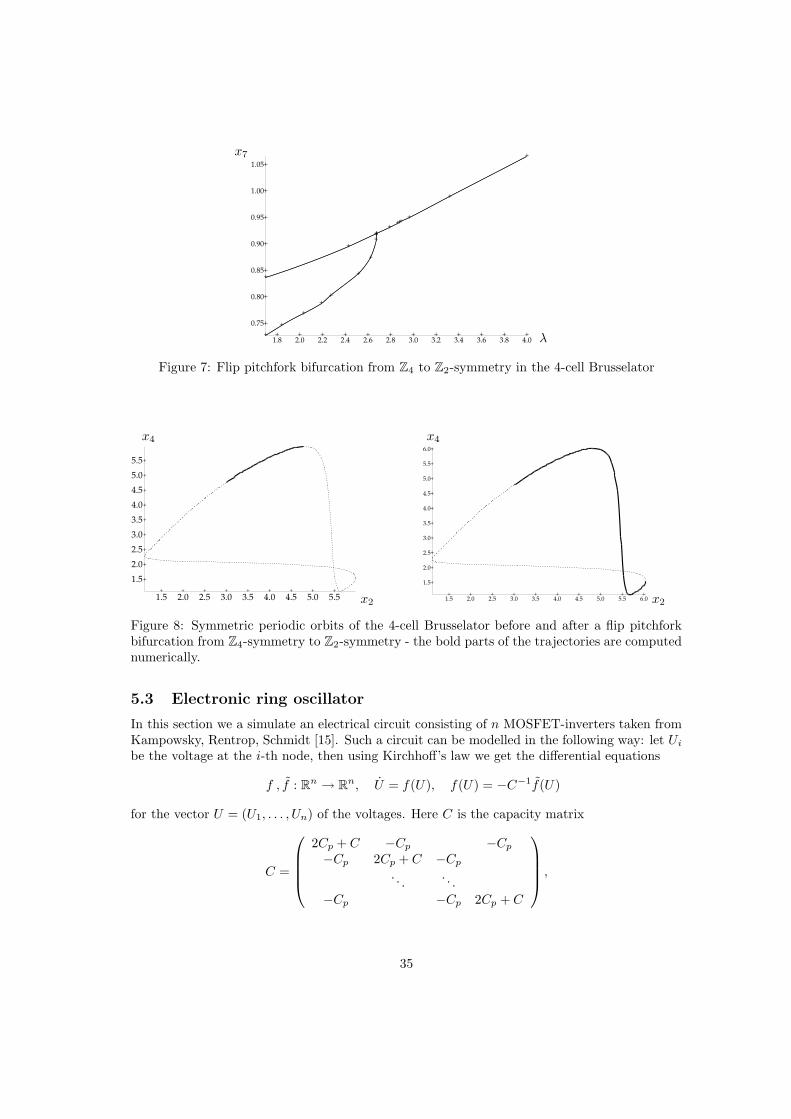
1.8 2.0 2.2 2.4 2.6 2.8 3.0 3.2 3.4 3.6 3.8 4.0

0.75

0.80

0.85

0.90

0.95

1.00

1.05

+ + + + + + + + + + + +

+

+

+

+

+

+

+

x7

λ

Figure 7: Flip pitchfork bifurcation from Z4 to Z2-symmetry in the 4-cell Brusselator

1.5 2.0 2.5 3.0 3.5 4.0 4.5 5.0 5.5

1.5

2.0

2.5

3.0

3.5

4.0

4.5

5.0

5.5

+ + + + + + + + +

+

+

+

+

+

+

+

+

+

1.5 2.0 2.5 3.0 3.5 4.0 4.5 5.0 5.5 6.0

1.5

2.0

2.5

3.0

3.5

4.0

4.5

5.0

5.5

6.0

+ + + + + + + + + +

+

+

+

+

+

+

+

+

+

+

x2

x4

x2

x4

Figure 8: Symmetric periodic orbits of the 4-cell Brusselator before and after a flip pitchforkbifurcation from Z4-symmetry to Z2-symmetry - the bold parts of the trajectories are computednumerically.

5.3 Electronic ring oscillator

In this section we a simulate an electrical circuit consisting of n MOSFET-inverters taken fromKampowsky, Rentrop, Schmidt [15]. Such a circuit can be modelled in the following way: let Ui

be the voltage at the i-th node, then using Kirchhoff’s law we get the differential equations

f , f : Rn → R

n, U = f(U), f(U) = −C−1f(U)

for the vector U = (U1, . . . , Un) of the voltages. Here C is the capacity matrix

C =

2Cp + C −Cp −Cp

−Cp 2Cp + C −Cp

. . .. . .

−Cp −Cp 2Cp + C

,

35

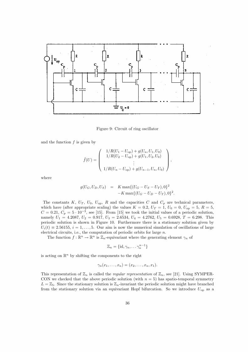
Figure 9: Circuit of ring oscillator

and the function f is given by

f(U) =

1/R(U1 − Uop) + g(Un, U1, U0)1/R(U2 − Uop) + g(U1, U2, U0)

...1/R(Un − Uop) + g(Un−1, Un, U0)

,

where

g(UG, UD, US) = K max{(UG − US − UT ), 0}2

−K max{(UG − UD − UT ), 0}2.

The constants K, UT , U0, Uop, R and the capacities C and Cp are technical parameters,which have (after appropriate scaling) the values K = 0.2, UT = 1, U0 = 0, Uop = 5, R = 5,C = 0.21, Cp = 5 · 10−3, see [15]. From [15] we took the initial values of a periodic solution,namely U1 = 4.2087, U2 = 0.917, U3 = 2.6534, U4 = 4.2762, U5 = 0.6928, T = 6.298. Thisperiodic solution is shown in Figure 10. Furthermore there is a stationary solution given byUi(t) ≡ 2.56155, i = 1, . . . , 5. Our aim is now the numerical simulation of oscillations of largeelectrical circuits, i.e., the computation of periodic orbits for large n.

The function f : Rn → Rn is Zn-equivariant where the generating element γn of

Zn = {id, γn, . . . γn−1n }

is acting on Rn by shifting the components to the right

γn(x1, . . . , xn) = (x2, . . . , xn, x1).

This representation of Zn is called the regular representation of Zn, see [21]. Using SYMPER-CON we checked that the above periodic solution (with n = 5) has spatio-temporal symmetryL = Z5. Since the stationary solution is Zn-invariant the periodic solution might have branchedfrom the stationary solution via an equivariant Hopf bifurcation. So we introduce Uop as a

36

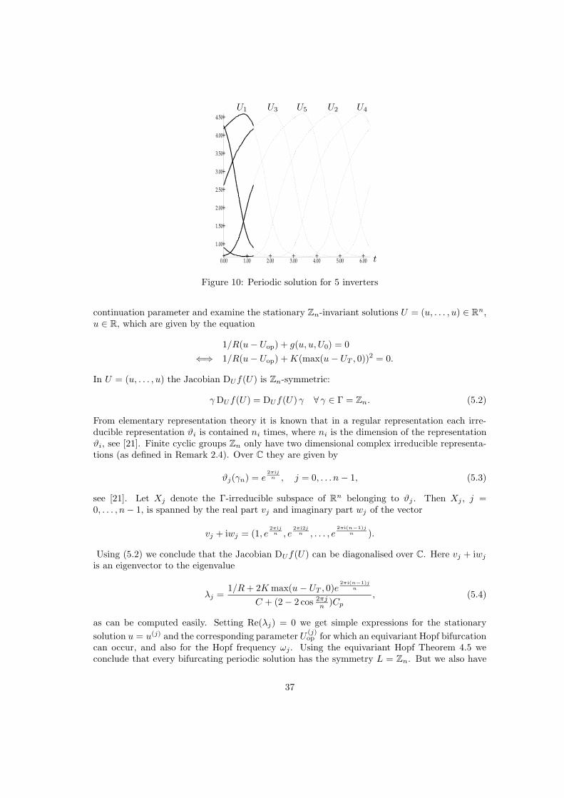
0.00 1.00 2.00 3.00 4.00 5.00 6.00

1.00

1.50

2.00

2.50

3.00

3.50

4.00

4.50

+ + + + + + ++

+

+

+

+

+

+

+

t

U1 U3 U5 U2 U4

Figure 10: Periodic solution for 5 inverters

continuation parameter and examine the stationary Zn-invariant solutions U = (u, . . . , u) ∈ Rn,u ∈ R, which are given by the equation

1/R(u− Uop) + g(u, u, U0) = 0

⇐⇒ 1/R(u− Uop) + K(max(u − UT , 0))2 = 0.

In U = (u, . . . , u) the Jacobian DUf(U) is Zn-symmetric:

γ DU f(U) = DUf(U) γ ∀ γ ∈ Γ = Zn. (5.2)

From elementary representation theory it is known that in a regular representation each irre-ducible representation ϑi is contained ni times, where ni is the dimension of the representationϑi, see [21]. Finite cyclic groups Zn only have two dimensional complex irreducible representa-tions (as defined in Remark 2.4). Over C they are given by

ϑj(γn) = e2πij

n , j = 0, . . . n − 1, (5.3)

see [21]. Let Xj denote the Γ-irreducible subspace of Rn belonging to ϑj . Then Xj , j =0, . . . , n − 1, is spanned by the real part vj and imaginary part wj of the vector

vj + iwj = (1, e2πij

n , e2πi2j

n , . . . , e2πi(n−1)j

n ).

Using (5.2) we conclude that the Jacobian DUf(U) can be diagonalised over C. Here vj + iwj

is an eigenvector to the eigenvalue

λj =1/R + 2K max(u − UT , 0)e

2πi(n−1)jn

C + (2 − 2 cos 2πjn )Cp

, (5.4)

as can be computed easily. Setting Re(λj) = 0 we get simple expressions for the stationary

solution u = u(j) and the corresponding parameter U(j)op for which an equivariant Hopf bifurcation

can occur, and also for the Hopf frequency ωj . Using the equivariant Hopf Theorem 4.5 weconclude that every bifurcating periodic solution has the symmetry L = Zn. But we also have

37

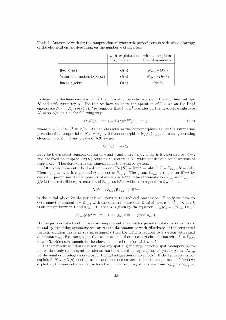
Table 1: Amount of work for the computation of symmetric periodic orbits with trivial isotropyof the electrical circuit depending on the number n of inverters

with exploitationof symmetry

without exploita-tion of symmetry

flow Φt(x) O(n) Nstep ∗ O(n)

Wronskian matrix DxΦt(x) O(n) Nstep ∗ O(n2)

linear algebra O(n) O(n3)

to determine the homomorphism Θ of the bifurcating periodic orbits and thereby their isotropyK and drift symmetry α. For this we have to know the operation of Γ × S1 on the Hopfeigenspace Nω∗ = Xj , see (4.6). We compute that Γ × S1 operates on the irreducible subspaceXj = span(vj , wj) in the following way

(γ, θ)(vj + iwj) = ϑj(γ)e2πiθ(vj + iwj), (5.5)

where γ ∈ Γ, θ ∈ S1 ≡ R/Z. We can characterize the homomorphism Θj of the bifurcatingperiodic orbits tangential to Nω∗ = Xj by the homomorphism Θj(γn) applied to the generatingelement γn of Zn. From (5.5) and (5.3) we get

Θj(γn) = −j/n.

Let r be the greatest common divisor of n and j and nred := n/r. Then K is generated by γnredn ,

and the fixed point space Fix(K) contains all vectors in Rn which consist of r equal sections oflength nred. Therefore nred is the dimension of the reduced system.

After restriction onto the fixed point space Fix(K) = Rnred we obtain L = Znred, K = {id}.

Then γnred≡ γnK is a generating element of Znred

. The group Znredalso acts on Rnred by

cyclically permuting the components of every x ∈ Rnred . The representation ϑjred with jred :=

j/r is the irreducible representation of Znredon Rnred which corresponds to ϑj . Thus,

N redω∗ = 〈Vjred , Wjred 〉 ⊂ R

nred

is the initial plane for the periodic solutions in the reduced coordinates. Finally we have todetermine the element α ∈ Znred

with the smallest phase shift Θred(α). Let α = γknred

, where kis an integer between 1 and nred − 1. Then α is given by the equation Θred(α) = 1/nred, i.e.,

ϑjred (α)e2πi/nred = 1 ⇔ jred k ≡ 1 (mod nred).

By the just described method we can compute initial values for periodic solutions for arbitraryn, and by exploiting symmetry we can reduce the amount of work effectively: if the consideredperiodic solution has large spatial symmetry then the ODE is reduced to a system with smalldimension nred. For example, in the case n = 1000, there is a periodic solution with K = Z200,nred = 5, which corresponds to the above computed solution with n = 5.

If the periodic solution does not have any spatial symmetry, but only spatio-temporal sym-metry then only the integration interval can be reduced by exploitation of symmetry. Let Nstep

be the number of integration steps for the full integration interval [0, T ]. If the symmetry is notexploited, Nstep ∗O(n) multiplications and divisions are needed for the computation of the flow;exploiting the symmetry we can reduce the number of integration steps from Nstep to Nstep/n,

38

since the integration interval is only [0, T/n]. Hence for large n the number of time steps is O(1),and so the number of multiplications and divisions for the computation of the flow is O(n) whensymmetry is exploited. Since the derivatives Dxf(x) are tridiagonal matrices and hence containonly O(n) non-zero components, Nstep ∗ O(n2) multiplications are needed for the computationof the Wronskian matrices DxΦt(x) by integration of the variational equation if the symmetryis not exploited; if the symmetry is exploited then for large n only few steps of integration arenecessary for the computation of the Wronskian matrices. Therefore the Wronskian matricesare sparse, and only contain non-zero entries close to the diagonal. Hence by exploitation ofsymmetry the amount of work for the computation of the Wronskian reduces to O(n). For the so-lution of the linear equations which arise in the Gauss-Newton method O(n3) multiplications areneeded if the symmetry is not exploited, and the amount of work for the linear algebra reducesto O(n) due to the sparse structure of the Wronskians if the symmetry is exploited. Altogetherwe obtain a remarkable reduction of the computational cost by exploitation of symmetry, c.f.Table 1.

Conclusion and future directions

In this paper we have presented efficient algorithms for the computation of generic symmetrychanging but isotropy preserving bifurcations of periodic orbits in systems where the symmetrygroup is discrete. These bifurcations were analyzed by Golubitsky et al (equivariant Hopf bifur-cation, see eg [11]) and Fiedler (flip doubling and flip pitchfork bifurcations, see [9]). Generalsymmety breaking bifurcations of periodic orbits in systems with discrete symmetry group wereclassified by Lamb and Melbourne [18], see also [19] and [24] for the case of continuous symme-try groups. In future work we will extend our numerical results to compute symmetry changingbifurcations of periodic orbits of arbitrary Lie group actions. In the paper [26] we extend themethods presented here to Hamiltonian systems with continuous symmetries building on thepersistence results of [25].

References

[1] W.-J. Beyn, A. Champneys, E. Doedel, W. Govaerts, Y. A. Kuznetsov, B. Sandstede.Numerical continuation, and computation of normal forms. Chapter 4 of Handbook ofDynamical Systems, vol. 2, B. Fiedler ed., pp. 149–219, 2002.

[2] K. A. Cliffe, A. Spence, and S. J. Tavener. O(2)-symmetry breaking bifurcation: withapplication to the flow past a sphere in a pipe. Internat. J. Numer. Methods Fluids 32(2):175–200, 2000.

[3] M. Dellnitz. A computational method and pathfollowing for periodic solutions with sym-metry. In D. Roose, B. de Dier, A.Spence, ed., Continuation and Bifurcations: NumericalTechniques and Applications, NATO ASI SERIES C, vol. 313, pp. 153–167, 1990.

[4] M. Dellnitz. Computational bifurcation of periodic solutions in systems with symmetry.IMA Journal of Numerical Analysis, 12: 429–455, 1992.

[5] P. Deuflhard. Computation of periodic solutions of nonlinear ODE’s. BIT 24: 456–466,1984.

[6] P. Deuflhard. Recent progress in extrapolation methods for ordinary differential esquations.SIAM Review 27: 505-535, 1985.

39

[7] P. Deuflhard, B. Fiedler, P. Kunkel. Efficient numerical pathfollowing beyond critical points.SIAM J. Numer. Anal., 18: 949–987, 1987.

[8] E.J. Doedel, R.C. Paffenroth, A.R. Champneys, T.F. Fairgrieve, Y.A. Kuznetsov, B.E.Oldeman, B. Sandstede and X.-J. Wang. AUTO2000: Continuation and bifurcation softwarefor ordinary differential equations. Technical Report, Concordia University 2000, availablefrom http://www.cs.concordia.ca.

[9] B. Fiedler. Global Bifurcation of Periodic Solutions with Symmetry. Lecture Notes inMathematics. Springer Verlag, Berlin, Heidelberg, New York, 1988.

[10] K. Gatermann, A. Hohmann. Symbolic exploitation of symmetry in numerical pathfollow-ing. IMPACT Comput. Sci. Engrg. 3: 330–365, 1991.

[11] M. Golubitzky, I. Stewart, D. Schaeffer. Singularities and Groups in Bifurcation Theory,volume 2. Springer-Verlag, Berlin, Heidelberg, New York, 1988.

[12] A. Griewank and G. W. Reddien. The calculation of Hopf points by a direct method. IMAJ. Numer. Anal. 3: 295–303, 1983.

[13] J. Guckenheimer and P. Holmes. Nonlinear Oscillations, Dynamical Systems, and Bifurca-tions of Vector Fields, Applied Mathematical Sciences, vol. 42. Springer-Verlag, New York,Heidelberg, Berlin, 1990.

[14] A. D. Jepson. Numerical Hopf Bifurcation. PhD thesis, California Institute of Technology,1981.

[15] W. Kampowsky, P. Rentrop, W. Schmidt. Classification and numerical simulation of electriccircuits. Surveys on Mathematics for Industry, 2(1): 23–65, 1992.

[16] Y. Kuznetsov. Elements of Applied Bifurcation Theory. Applied Mathematical Sciences,vol. 112. Springer, New York, 1995.

[17] Y.A. Kuznetsov and V.V. Levitin. CONTENT: A multiplatform environment for continua-tion and bifurcation analysis of dynamical systems. Centrum voor Wiskunde en Informatica1997, available from ftp://ftp.cwi.nl/pub/CONTENT.

[18] J. S. W. Lamb and I. Melbourne. Bifurcation from discrete rotating waves. ArchiveRat. Mech. Anal. 149: 229–270, 1999.

[19] J. Lamb, I. Melbourne, C. Wulff. General bifurcations from periodic solutions with spa-tiotemporal symmetry, including mode interactions and resonances. J. Differential Equa-tions, 191(2): 377–407, 2003.

[20] A. Schebesch. SYMPERCON - a package for the numerical continuation of symmetricperiodic orbits. Diplomarbeit, Freie Universitat Berlin, 2004. The current version of SYM-PERCON can be obtained from http://www.maths.surrey.ac.uk/personal/st/C.Wulff/.

[21] J.-P. Serre. Linear Representations of Finite Groups. Springer-Verlag, New York, Heidel-berg, Berlin, 1977.

[22] C. Wulff. Numerische Pfadverfolgung von periodischen Losungen mit Symmetrie. Di-plomarbeit, Freie Universitat Berlin, 1993.

[23] C. Wulff, A. Hohmann, P. Deuflhard. Numerical continuation of periodic orbits with sym-metry. Technical report, Konrad-Zuse-Zentrum, Berlin, 1994.

40

[24] C. Wulff, J. Lamb, I. Melbourne. Bifurcation from relative periodic solutions. Er-godic Th. Dyn. Syst. 21: 605–635, 2001.

[25] C. Wulff. Persistence of Hamiltonian relative periodic orbits. J. Geom. Phys. 48: 309-338,2003.

[26] C. Wulff and A. Schebesch. Numerical continuation of Hamiltonian relative periodic orbits.Preprint.

41