

Numerical experiments with
an interior-exterior point method
for nonlinear programming
Igor Griva ∗
April 12, 2004
Abstract
The paper presents an algorithm for solving nonlinear program-ming problems. The algorithm is based on the combination of interiorand exterior point methods. The latter is also known as the primal-dual nonlinear rescaling method. The paper shows that in certaincases when the interior point method (ipm) fails to achieve the so-lution with the high level of accuracy, the use of the exterior pointmethod (epm) can remedy this situation. The result is demonstratedby solving problems from cops and cute problem sets using nonlin-ear programming solver loqo that is modified to include the exteriorpoint method subroutine.
Keywords. Interior point method, exterior point method, primal-dual, nonlinear rescaling.
1 Introduction.
This paper considers a method for solving the following optimization problem
min f(x),
s.t. h(x) ≥ 0,(1)
∗Princeton University, Department of ORFE, Princeton NJ 08544, Email:[email protected]
1

where h(x) = (h1(x), . . . , hm(x)) is a vector function. We assume that
f : IRn → IR1 and all hi : IRn → IR1, i = 1, . . . , m are twice continuously
differentiable functions.
To solve this problem we use a method based on the combination of inte-
rior and exterior point methods. We describe these methods in the following
sections. This section explains both interior and exterior point methods in
the context of their development. It illustrates how the two methods are re-
lated and why their integration is a reasonable approach for solving nonlinear
programming problems.
In the past two decades interior point methods have proven to be efficient
and are widely used for solving linear and nonlinear programming problems.
The interior point methods are closely related to the sequential uncon-
strained minimization technique (sumt) developed by Fiacco and McCormick
[4] for solving constrained optimization problem with inequality constraints.
The sequential unconstrained minimization technique is based on a sequence
of unconstrained minimizations of the classical log-barrier function followed
by the barrier parameter update.
Among all variations of interior point methods related to sumt, the
primal-dual interior point method is the most efficient. At each step it solves
the primal-dual system equivalent to the optimality criteria for the minimiza-
tion of the classical log-barrier function. Since the late 1980s the primal-dual
interior point method has become the most popular algorithm for large scale
linear programming. It has solid a theoretical foundation and is computa-
tionally efficient. The developed theory and numerical experiments revealed
that the primal-dual interior point method shows excellent performance for
large scale practical problems [9, 22]. The performance of the primal-dual
interior point method on nonlinear programming problems is robust. The
2

algorithm shows solid global convergence properties.
The primal-dual interior point method overcame well-known difficulties
associated with the sequential unconstrained minimization technique. Of
particular importance is that the efficiency of sumt is compromised by the
singularity of the classical barrier function and its derivatives at the solution,
which makes it difficult to use methods of unconstrained minimization effec-
tively. The primal-dual interior point method suffers the least of any other
variation of the interior point methods from the ill-conditioning. Neverthe-
less, for certain problems even the primal-dual interior point method fails to
achieve the desired level of accuracy.
The problems associated with the sequential unconstrained minimization
technique encouraged the optimization community to look for alternatives.
Thus in the early 1980s Polyak [12] suggested a different approach for solving
constrained optimization problems with inequality constraints. He developed
the theory of modified barrier functions (mbf) and the corresponding modi-
fied barrier function methods . Independently, in 1970s Kort and Bertsekas
[8] introduced the exponential multipliers method. Both modified barrier
function and exponential multipliers methods are particular cases of the non-
linear rescaling principle [13, 15].
The nonlinear rescaling principle consists of a sequence of unconstrained
minimizations of the Lagrangian for the equivalent problem followed by the
Lagrange multipliers update. Later, keeping in mind the theoretical and nu-
merical success related to the primal-dual interior point methods, there was
motivation to develop the primal-dual method based on the nonlinear rescal-
ing theory, which is an exterior point method (epm). Instead of performing
a sequence of unconstrained minimizations, the exterior point method solves
the primal-dual system by Newton’s method [7, 14, 16]. In general, the
3

trajectory of the exterior point method approaches the solution outside the
feasible set.
The exterior point method allows for simultaneous computation of the
primal and the dual approximations. Furthermore, the epm has interesting
local convergence properties. Under the standard second order optimality
conditions the exterior point method converges with a linear rate under the
fixed barrier parameter [16]. If the barrier parameter decreases at each step,
the rate of convergence of the exterior point method is superlinear [7]. Locally
the exterior point method has a trajectory similar to that of Newton’s method
applied to the Lagrange system of equations that correspond to the active
constraints [7].
Taking into account the robustness and the global convergence properties
of the interior point method and the fast local convergence properties of the
exterior point method, these two methods can potentially augment each other
and result in a more robust combination: an interior-exterior point method
(iepm). The main idea of this paper is to develop an algorithm based on
such a combination and test it on a variety of problems. We incorporated
the exterior point method into the general nonconvex nonlinear programming
solver loqo, which is based on the primal-dual interior point method.
The interior point algorithm for nonconvex nonlinear programs, imple-
mented in loqo, has been described and studied in [1, 19, 20, 21]. The
appropriate choice of a filter or a merit function together with regularization
of a Hessian of the Lagrangian [19] contributes to the global convergence
of the interior point algorithm. In some cases, however, the interior point
method experiences numerical problems when approaching the solution. In
this paper we propose to switch to the exterior point method, which has fast
local convergence properties [7, 16], when the numerical problems occur.
4

The structure of the matrices for the Newton directions in the interior
and exterior point methods are identical. Therefore the sparse linear algebra
developed by Vanderbei [18] for loqo, can be used in both methods.
The paper is organized as follows. In the next section we describe briefly
the interior point algorithm implemented in loqo and its connection to the
sequential unconstrained minimization technique. In section 3 we discuss
the exterior point method in connection to the nonlinear rescaling principle.
Section 4 describes the interior-exterior point method (iepm) and presents
the numerical results for testing iepm on cops [2] and cute [3] problem
sets. Section 5 contains the discussion of numerical results and concluding
remarks.
2 The interior point method.
We will focus on the minimization problem with inequality constraints (1).
Equality constraints can be included in the formulation, but we ignore them
to simplify the presentation. Let us consider the following optimization prob-
lem. Applying the classical log-barrier function to problem (1) we obtain
B(x, µ) = f(x) − µm
∑
i=1
lnhi(x),
where µ > 0 is a barrier parameter.
Sequential unconstrained minimization technique replaces a constrained
optimization problem with a sequence of unconstrained optimization prob-
lems. Assuming that log t = −∞, t ≤ 0 we obtain
x(µ) = argmin{B(x, µ)|x ∈ IRn} (2)
Solving problem (2) sequentially for a monotoneously decreasing sequence
{µk} such that limk→∞ µk = 0 gives a sequence {x(µk)} yielding h(x(µk)) > 0
and limk→∞ f(x(µk)) = f(x∗), where x∗ is the solution of the problem (1).
5

To find the minimum of B(x, µ) in x is equivalent to solving the system
∇xB(x, µ) = ∇f(x) − µm
∑
i=1
∇hi(x)
hi(x)= 0 (3)
Let x(µ) : ∇B(x(µ), µ) = 0 and yi(µ) = µ/hi(x(µ)), i = 1, . . . , m. Therefore
the pair (x(µ), y(µ)) is the solution of the following primal-dual system of
equations
∇L(x, y) = ∇f(x) −m
∑
i=1
yi∇hi(x) = 0, (4)
yihi(x) = µ, i = 1, . . . , m, (5)
where L(x, y) = f(x) −∑m
i=1 yihi(x) is the Lagrangian of the problem (1).
The primal or primal-dual interior point methods perform one Newton
step towards the solution of systems (3) or (4)-(5) respectively followed by
changing the barrier parameter µ. Therefore there are similarities and dif-
ferences between the sequential unconstrained minimization technique and
interior point methods. The methods are related to each other because they
both rely on the primal-dual central path (x(µ), y(µ)) introduced by Fiacco
and McCormick in the 1960s. In the late 1980s and early 1990s, when interior
point methods emerged as popular methods in optimization it became evi-
dent that the central path is also the main component of IPM developments
[10]. The key difference between interior point methods and the sequential
unconstrained minimization technique is in the role Newton’s method plays
in their frameworks. In the sequential unconstrained minimization technique
Newton’s method is used for the unconstrained minimizations, which result
in approximations of the central path. After each minimization the bar-
rier parameter is decreased. Interior point methods usually perform just
one Newton step for the system similar to (4)-(5) toward the central path
followed by the barrier parameter update. For efficiency of interior point
methods it is critical to keep their trajectory in the intersection of an interior
6

of the feasible set and the Newton area, the area where Newton’s method
is well defined [17]. The size of this intersection generally depends on the
value of the barrier parameter. Whereas for the sequential unconstrained
minimization technique the rate of change of the barrier parameter is not a
key issue, an uncontrolled change of the barrier parameter could compromise
the efficiency of interior point methods.
The interest in the central path, the classical barrier function and the cor-
responding methods has been revived in the course of linear programming
development [9, 22], especially after the recognition of the role that New-
ton’s method plays in interior point methods [6]. IPMs have proven to be
efficient and widely used for LP. The success of interior point methods in lin-
ear programming sparked the interest to applying the methods for nonlinear
programming.
Let us briefly describe the interior point method implemented in loqo.
By introducing nonnegative slack variables w = (w1, . . . , wm), the problem
(2) can be replaced by the following problem
min f(x) − µm∑
i=1logwi,
s.t. h(x) − w = 0,
(6)
where µ > 0 is a barrier parameter. The solution of this problem satisfies
the following primal-dual system
∇f(x) −∇h(x)Ty = 0,−µe+WY e = 0,
h(x) − w = 0,(7)
where y = (y1, . . . , ym) is a vector of the Lagrange multipliers or dual vari-
ables for problem (6), ∇h(x) is the Jacobian of vector function h(x), Y
and W are diagonal matrices with elements yi and wi respectively and e =
(1, . . . , 1) ∈ IRm.
7

Applying Newton’s method to the system (7) leads to the following linear
system for the Newton directions
∇2xxL(x, y) 0 −∇h(x)T
0 Y W∇h(x) −I 0
∆x∆w∆y
=
−∇f(x) + ∇h(x)Tyµe−WY e−h(x) + w
,
where ∇2xxL(x, y) = ∇2f(x)−
∑mi=1 yi∇
2hi(x) is the Hessian of the Lagrangian
of problem (1). After eliminating ∆w from this system we obtain the follow-
ing reduced system
[
−∇2xxL(x, y) ∇h(x)T
∇h(x) WY −1
] [
∆x∆y
]
=
[
σρ+WY −1γ
]
, (8)
where
σ = ∇f(x) −∇h(x)T y,
γ = µW−1e− y,
ρ = w − h(x).
Then we can find ∆w by the following formula
∆w = WY −1(γ − ∆y).
One step of the IPM algorithm (x, w, y) → (x, w, y) is as follows
x = x+ α∆x,
w = w + α∆w,
y = y + α∆y,
where α is a steplength chosen according to a merit function [19] or a filter
method [1, 5] and to keep the slacks wi and Lagrange multipliers yi positive.
8

If the Hessian ∇2xxL(x, y) is not positive definite the algorithm replaces
it with the regularized Hessian
Rλ(x, y) = ∇2xxL(x, y) + λI, λ ≥ 0,
where I is the identity matrix in IRn,n. The regularization prevents conver-
gence to a local maximum. Parameter λ is chosen big enough to guarantee
that the regularized Hessian H(x, y) is positive definite. The interior point
method generates a sequence {xk, wk, yk} as described above for a sequence
of positive barrier parameters {µk} converging to zero.
The detailed description of the algorithm can be found in [1, 19, 20, 21].
We draw the reader’s attention, however, to the fact that the sequence of
slack variables {wk} is required to stay positive throughout the computa-
tion. Starting with a strictly positive vector w0, the interior point algorithm
chooses the steplength small enough to keep the slack variables and Lagrange
multipliers positive and, thus, prevents the trajectory of the method from hit-
ting the boundary of the feasible set. When there is a risk for the slacks to
become zero, the algorithm reduces the steplength.
Sometimes, however, the steplength becomes too small, which compro-
mises the convergence of the algorithm. When this happens, we switch to
the exterior point method. The trajectory of the exterior point method is
allowed to leave the feasible set. Therefore it is not necessary to keep the
slack variables positive. Usually, the trajectory of the exterior point method
approaches solution outside of the feasible set.
3 The exterior point method.
The exterior point methods are related to the nonlinear rescaling principle
the same way as the interior point methods are related to the sequential
9

unconstrained minimization technique. The exterior point method is also
known as the primal-dual nonlinear rescaling method and described in [7, 16].
Here we just review its basic principles.
Let −∞ ≤ t0 < 0 < t1 ≤ ∞. We consider a class Ψ of twice continuously
differential functions ψ : (t0, t1) → IR that satisfy the following properties
10. ψ(0) = 0.
20. ψ′(t) > 0.
30. ψ′(0) = 1.
40. ψ′′(t) < 0.
50. there is a > 0 such that ψ(t) ≤ −at2, t ≤ 0.
60. a) ψ′(t) ≤ bt−1, b) −ψ′′(t) ≤ ct−2, t > 0, b > 0, c > 0.
Let us consider a few transformations ψ ∈ Ψ.
1. Exponential transformation [8]
ψ1(t) = 1 − e−t.
2. Logarithmic modified barrier function [12]
ψ2(t) = log(t+ 1).
3. Hyperbolic modified barrier function [12]
ψ3(t) =t
1 + t.
The exponential transformation ψ1(t) leads to the exponential multipliers
method while the logarithmic and hyperbolic transformations lead to the
modified barrier function method. In this paper we use the logarithmic
modified barrier function ψ(t) = ψ2(t) = log(t + 1) to conduct numerical
experiments.
We transform the constraints of problem (1) into an equivalent set of
constraints using functions ψ ∈ Ψ.
10

For any given transformation ψ ∈ Ψ and any barrier parameter µ > 0
due to 10 − 30 the following problem is equivalent to problem (1)
min f(x),
s.t. µψ (µ−1hi(x)) ≥ 0, i = 1, . . . , m.
(9)
The classical Lagrangian L : IRn×IRm+×IR1
++ → IR1 for the equivalent problem
(9) that is given by formula
L(x, y, µ) = f(x) − µm
∑
i=1
yiψ(µ−1hi(x)).
is the main tool for the nonlinear rescaling method. One step of the nonlinear
rescaling method maps the given approximation (x, y) to the next (x, y) by
the following formulas
x = argmin {L(x, y, µ) | x ∈ IRn} , (10)
yi = ψ′(
µ−1hi(x))
yi, i = 1, . . . , m. (11)
The Lagrangian for the equivalent problem L(x, y, µ) plays in nonlinear
rescaling theory a similar role to that the classical barrier function B(x, µ)
plays in the sequential unconstrained minimization technique. But unlike
the classical barrier function, the Lagrangian for the equivalent problem
L(x, y, µ) in addition to the barrier parameter also depends on the Lagrange
multipliers associated with each constraint. When based on the logarithmic
modified barrier function ψ2(t), the Lagrangian for the equivalent problem
retains the most important properties of the classical barrier function, e.g.
self-concordance [11]. This gives similar complexity results for the method
with the fixed Lagrange multipliers and decreasing barrier parameter [12]. At
the same time, the nonlinear rescaling principle eliminates the main problems
of the sequential unconstrained minimization technique associated with the
11

singularity of the classical barrier function B(x, µ) and its derivatives at the
solution. In particular, the nonlinear rescaling method keeps stable the New-
ton area for unconstrained minimization and exhibits the “hot start” phe-
nomenon [12] under the standard second order optimality conditions: from
some point along the trajectory the primal approximation remains in the
area where Newton’s method is well defined after each Lagrange multipliers
update.
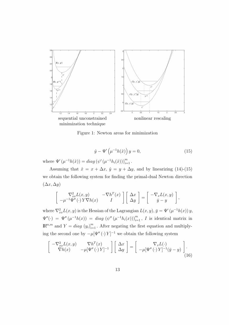
Figure 1 demonstrates the sequential unconstrained minimization tech-
nique and the nonlinear rescaling principle for the following problem
min x2,
s.t.
x ≥ 1, x ≥ 0.
The solution of this problem is x∗ = 1. The area where Newton’s method is
well defined for minimization of the classical log-barrier function shrinks to
a point near the solution while the Newton area for the minimization of the
Lagrangian L(x, y, µ) for the equivalent problem stays stable.
The exterior point method was developed to avoid unconstrained mini-
mization at each step. One step of the nonlinear rescaling method (10)-(11)
is equivalent to solving the for (x, y) the following primal-dual system
∇xL(x, y, µ) = ∇f(x) −m
∑
i=1
ψ′(
µ−1hi(x))
yi∇hi(x) = 0, (12)
yi = ψ′(
µ−1hi(x))
yi, i = 1, . . . , m. (13)
After replacing the terms ψ′ (µ−1hi(x)) yi in (12) by yi, i = 1, . . . , m, we
obtain another equivalent nonlinear system
∇xL(x, y) = ∇f(x) −m
∑
i=1
yi∇hi(x) = 0, (14)
12
1.2 1.4 1.6 1.8 2 2.2 2.4
1
1.2
1.4
1.6
1.8
2
2.2
2.4
2.6
2.8
0 0.5 1 1.5 2 2.5 3-0.5
0
0.5
1
1.5
2
2.5
3
*
xs
sequential unconstrained nonlinear rescalingminimization technique
Figure 1: Newton areas for minimization
y − Ψ′(
µ−1h(x))
y = 0, (15)
where Ψ′ (µ−1h(x)) = diag (ψ′ (µ−1hi(x)))m
i=1 .
Assuming that x = x + ∆x, y = y + ∆y, and by linearizing (14)-(15)
we obtain the following system for finding the primal-dual Newton direction
(∆x,∆y)
[
∇2xxL(x, y) −∇hT (x)
−µ−1Ψ′′ (·) Y∇h(x) I
] [
∆x∆y
]
=
[
−∇xL(x, y)y − y
]
,
where ∇2xxL(x, y) is the Hessian of the Lagrangian L(x, y), y = Ψ′ (µ−1h(x)) y,
Ψ′′(·) = Ψ′′ (µ−1h(x)) = diag (ψ′′ (µ−1hi(x)))m
i=1 , I is identical matrix in
IRm,m and Y = diag (yi)m
i=1 . After negating the first equation and multiply-
ing the second one by −µ[Ψ′′ (·)Y ]−1 we obtain the following system
[
−∇2xxL(x, y) ∇hT (x)∇h(x) −µ[Ψ′′ (·)Y ]−1
] [
∆x∆y
]
=
[
∇xL(·)−µ[Ψ′′ (·)Y ]−1(y − y)
]
.
(16)
13

In particular, for the transformation ψ(t) = log(t+1) used for the numerical
experiments in this paper, system (16) becomes[
−∇2xxL(x, y) ∇hT (x)∇h(x) µ−1[H(x) + µI]2Y −1
] [
∆x∆y
]
=
[
∇xL(·)µ−1[H(x) + µI]2Y −1(y − y)
]
,
where H(x) = diag (hi(x))mi=1.
One step of the exterior point method updates the current primal-dual
approximation as follows
x = x+ ∆x, (17)
y = y + ∆y. (18)
To avoid convergence to a local maximum we regularize the Hessian
∇2xxL(x, y) as before
Rλ(x, y) = ∇2xxL(x, y) + λI, λ ≥ 0.
The matrix in system (16) has the same structure and sparsity pattern as
those in system (8). Therefore we can use the sparse numerical linear algebra
technology developed in [18] for loqo.
Being efficient in the neighborhood of the primal-dual solution, method
(16)-(18) may not converge globally. To control the convergence we chose a
priori a factor 0 < q < 1 and introduce the merit function
ν(x, y) = max
{
‖∇xL(x, y)‖, − min1≤i≤m
hi(x), − min1≤i≤m
yi,m
∑
i=1
|yihi(x)|
}
, (19)
measuring the violation of the KKT conditions. It is shown in [16] that under
the standard second order optimality conditions for any a priori chosen factor
0 < q < 1 there is a neighborhood of the solution where the method (16)-
(18) converges linearly with this factor 0 < q < 1. Also, it is shown in [7]
that if functions f(x) and hi(x) are smooth enough then the merit function
converges to zero with the same rate.
14

We design the exterior point algorithm as follows. If one step of method
(16)-(18) does not reduce the value of the merit function ν(x, y) by the de-
sired factor 0 < q < 1, we assume that the switch from the interior point
method to method (16)-(18) is premature. In this case the trajectory of the
exterior point method is beyond the area of the linear convergence with this
factor 0 < q < 1. When it happens, the algorithm follows the trajectory of
the nonlinear rescaling method (10)-(11). We use the primal direction ∆x
obtained from system (16) for the first step of the minimizations (10). It is
shown in [7] that this direction is descending for the Lagrangian L(x, y, µ),
therefore the algorithm does not lose the computational work involved in
solving the system (16). Newton’s method with a steplength and the regu-
larized Hessian is used for the unconstrained minimization of the Lagrangian
(10) followed by the Lagrange multipliers update (11). The detailed descrip-
tion of this algorithm one can find in [7, 16]. Here we mention only that such
exterior point method is a globally convergent algorithm to a local minimum
for a wide class of problems [16]. Therefore, if the switch to the exterior
point method occurs while the trajectory of the algorithm is outside of the
area of linear convergence of epm with given factor 0 < q < 1, the nonlinear
rescaling method (10)-(11) will bring the trajectory to this area.
4 The interior-exterior point method: Nu-
merical results.
The main difference between the interior and exterior point methods is their
“driving force” of convergence. The former requires the decrease to zero of
the barrier parameter µ > 0. The latter converges due to the information car-
ried by the vector of the Lagrange multipliers y. The interior point method,
which has global convergence properties, exhibits robust behavior bringing
15

its trajectory to the neighborhood of the solution. Under the standard sec-
ond order optimality conditions the exterior point method converges in the
neighborhood of the solution with a linear rate under the fixed barrier pa-
rameter [16]. If the barrier parameter is decreased, the exterior point method
converges locally with the superlinear rate [7]. Therefore, the robustness of
the interior point method and the local convergence properties of the exte-
rior point method encourage us to consider the combination of the methods.
The methods can augment each other. Indeed, the interior point method can
bring the trajectory to the area of a superlinear convergence of the exterior
point method, while the exterior point method can improve the convergence
in case the interior point method experiences numerical problems.
It is important to properly define the switching rule between the interior
and exterior point methods. The ideal approach would be to characterize
the area of convergence of the exterior point method and to find a way to
verify whether the primal-dual trajectory is in this convergence area. This is
the subject of future research. Currently, we are using the following simple
consideration for the switching criteria.
The interior point method implemented in loqo produced strong results
on cops [2] and cute [3] problem sets. It solved 86.8% of the cops problems
and 85.1% of the cute problems with a default accuracy setting of 8 digits
of agreement between primal and dual objective functions and a primal-dual
infeasibility measure of 1e-6. So we decided to switch to the exterior point
method only if the interior point method stops making progress.
Although there is a chance of a false detection that the interior point
method is not making progress, the switching rule is still attractive due to its
simplicity. It allows us to test the hypothesis that the exterior point method
is capable of solving the problems that the interior point method cannot solve
16

alone and thus the combination of these two methods, the interior-exterior
point method (iepm) can solve more problems than the interior or exterior
point methods can individually.
To define the switching rule formally we use the merit function ν(x, y)
(19) that controls convergence of the algorithm. The switching rule from the
interior point method to the exterior point method is conservative. If for
seven consecutive iterations the interior point method does not reduce the
value of merit function ν(x, y) and the steplength α becomes less than the
requested accuracy of the solution, then the algorithm switches to the exterior
point method. In other words, we detect the “stalling” situations when
the algorithm fails to evolve. Also, the algorithm switches to the exterior
point method if for one third of the iteration limit the interior point method
does not reduce the best achieved value of the merit function ν(x, y), even
if the steplength is bigger than the requested accuracy. In other words,
the algorithm detects if there is no overall progress for a large number of
iterations. The interior-exterior point algorithm and the switching rule are
formally described in Figure 2.
Testing the interior-exterior point method on the cops set has resulted in
an increase of the number of solved problems from 59 to 64 out of 68. It means
reducing by more than half the number of unsolved problems. The additional
problems that the interior-exterior point method solved are Hanging chain
for nh = 200, Minimal surface with obstacle for ny = 100, linear tangent
particle steering for nh = 100, nh = 200 and nh = 400. The statistics for the
solutions of these problems are shown in Table 1. We show the solution time
in seconds, values of both primal and dual functions, both primal and dual
infeasibility and a number of iterations. If the iteration number exceeds 500,
we call the problem not solved.
17

Step 1: Initialization:
An initial primal approximation x0 ∈ IRn is given.Initial slacks w0 ∈ IRn
++ and Lagrange multipliers y0 ∈ IRm++ are given.
An accuracy parameter ε > 0 is given.Set (x,w, y) := (x0, w0, y0), rec := ν(x, y), it := 0, cnt1 := 0, cnt2 := 0.
Step 2: If r ≤ ε, Stop, Output: x, y.
Step 3: Find new (x, w, y) = IPMSTEP (x,w, y), it := it + 1.Step 4: If ν(x, y) ≤ ε, Stop, Output: x, y.
Step 5: If it = itlim, Stop, Output: Solution is not found.Step 6: If ν(x, y) ≤ 0.99ν(x, y) or steplength ≥ ε, Set cnt1 := 0, Goto Step 8.Step 7: Set cnt1 := cnt1 + 1.Step 8: If ν(x, y) ≤ 0.99rec, Set rec := ν(x, y), cnt2 := 0, Goto Step 10.Step 9: Set cnt2 := cnt2 + 1.Step 10: If cnt1 < 7 and 3 ∗ cnt2 < itlim, Set (x,w, y) := (x, w, y), Goto Step 3.Step 11: Find new (x, w, y) = EPMSTEP (x,w, y), it := it + 1.Step 12: If ν(x, w, y) ≤ ε, Stop, Output: x, y.
Step 13: If it = itlim, Stop, Output: Solution is not found.Step 14: Goto Step 11.
Figure 2: IEPM
Testing the method on the cute set increased the number of the solved
problems from 967 to 1003 out of 1135. If we increase the level of accuracy of
the solution to 12 digits of agreement between primal and dual functions and
infeasibility measure 1e-12, the interior point method solves 879 problems
and the interior-exterior point method solves 936, an improvement of 57
additional solved problems. It is appropriate to mention that the interior-
exterior point method actually solved 60 problems that have not been solved
by the interior point method. On the other hand the interior-exterior point
method did not solve 3 problems that the interior point method solved alone.
Tables 2-9 present the behavior of the algorithms. The tables show the
statistics of the problem, the primal and dual objective values, the primal
and dual infeasibility and the number of digits of agreement between the
primal and the dual functions, which characterizes the primal-dual gap.
18

chain Min surface linear tangent particle steeringnh = 200 ny = 100 nh = 100 nh = 200 nh = 400
time (sec) 44.01 90.81 7.89 11.29 24.07
pr. val = 5.068917340 2.506949256 0.554595401 0.554577016 0.554572413
dual val = 5.068917342 2.506949256 0.554595401 0.554577016 0.554572413
pr. inf = 3.5e-10 4.9e-09 5.7e-09 3.3e-11 1.3e-11
dual inf = 5.7e-11 4.1e-12 5.6e-10 1.4e-10 1.2e-10
steps 218 171 278 157 163
Table 1: COPS
Tables 2-4 demonstrate the superiority of the interior-exterior point method
over individual performance of the interior and exterior point methods. It
took 150 iterations of the interior point method to solve the problem trigger
(Table 2). The exterior point method by itself reached the iterations limit
due to its slow progress towards the solution (Table 3). However, the interior-
exterior point method solves the problem trigger in 55 iterations (Table 4).
Tables 5-8 show the behavior of the interior-exterior point method for
some problems. Table 5 shows the performance of the interior-exterior point
method for problem hager1. The interior point method had numerical dif-
ficulties reducing the dual infeasibility below 1e-4 while the exterior point
method achieved the desired level of accuracy in one iteration. Table 6
shows the performance of the interior-exterior point method for problem
spanhyd. The interior point method could not obtain the desired primal-
dual gap before the exterior point method attained it. The behavior of the
interior-exterior point method for problem ubh1 is shown in Table 7. Again,
the interior point method failed to improve the dual infeasibility beyond the
level of 1e-4, the exterior point method passed this threshold. Table 8 shows
the ability of the exterior point method to achieve very accurate solutions. To
demonstrate this we set the accuracy level to 12 digits of agreement between
the primal and dual functions and 1e-12 infeasibility tolerance.
It is common for the interior-exterior point method to exhibit higher pri-
19

mal infeasibility after switching to the exterior point method. It reflects the
effect of “open boundaries,” when the trajectory of the algorithm goes outside
of the feasible set to overcome the numerical problems in the neighborhood
of the solution. Afterwards, however, the primal and dual infeasibility, as
well as the duality gap, decrease with, at least, a linear rate.
Tables 5-8 show that the interior point method performs several steps
without any improvement before the exterior point method is used. These
“stalling” situations are simple to detect, however, in some cases the interior
point method does not make progress without exhibiting “stalling”. Such
a behavior of the interior point method occurs for the difficult nonconvex
nonlinear problems. The interior point method struggles to approach the
local minima and eventually succeeds in many cases. Using the exterior
point method prematurely can worsen the behavior of the algorithm. The
trajectory of the algorithm at this point can be far from the area of fast
convergence of the exterior point method therefore the algorithm exceeds the
limit of iterations. This is why the interior-exterior point method did not
solve several problems from the cute set, which the interior point method
could solve by itself. Nevertheless, using the exterior point method in loqo
has demonstrated an improvement.
Table 9 shows the performance of the interior-exterior point method for
the steering problem from the cops set with nh = 400. This problem ap-
peared to be difficult for the interior point method, while for the exterior
point method it took 8 iterations to obtain the solution with high accuracy.
This particular problem could be solved by the exterior point method alone
in 8 iterations. However, we used the same “conservative” switching rule for
all the tested problems. The interior point method implemented in loqo
is the robust algorithm and we advocate the strategy of giving the interior
20

point method the chance to converge by itself.
5 Concluding remarks.
The extensive numerical testing of the interior-exterior point method has
shown that the interior point method and the exterior point method are
capable of augmenting each other. Their combined performance is better
than either method can achieve individually.
One reason for the appearing of numerical problems that the interior
point method experience near the solution is related to the essential need
of the algorithm to keep slack variables positive and the ill-condition of the
system for finding the Newton directions. At the solution the values of slack
variables, corresponding to the active constraints are zero. Therefore, when
the trajectory of the interior point method approaches the solution the New-
ton directions must be computed very precisely to avoid premature annulling
of the slacks. However, the closer the trajectory of the interior point method
gets to the solution, the greater are the numerical errors. These errors occur
because of the ill-condition of the system for Newton directions (8). As a re-
sult, the steplength, which keeps the slacks positive, becomes very small and
numerical problems occur. On the other hand, the exterior point method is
less likely to exhibit such behavior. There is no need for the exterior point
method to keep slacks positive. The method allows the trajectory to leave the
interior of the feasible set. Also, the system for Newton directions is better
conditioned under the standard second order optimality conditions [7, 16].
The interior and exterior point methods stem from different ideologies.
The interior point method is closely related to the sequential unconstrained
minimization technique with the classical log-barrier function, while the exte-
rior point method is based on the nonlinear rescaling theory. However, both
21

variables: non-neg 0, free 6, bdd 0, total 6
constraints: eq 6, ineq 0, ranged 0, total 6
primal dual Sig
Iter Obj Value Infeas Obj Value Infeas Fig
interior point method...
1 0.000000e+00 1.1e+01 0.000000e+00 1.1e+01 60
2 0.000000e+00 1.4e-01 1.403131e+00 6.2e-02
3 0.000000e+00 1.2e-01 5.146799e-01 5.4e-02
4 0.000000e+00 4.0e-02 2.080966e-01 5.0e-02 1
..................................
24 0.000000e+00 1.4e-04 2.105166e-09 7.6e-05 9
..................................
44 0.000000e+00 4.9e-08 2.984260e-09 1.9e-04 9
..................................
64 0.000000e+00 5.3e-09 5.966625e-10 2.9e-05 9
..................................
84 0.000000e+00 7.9e-10 9.923364e-11 1.1e-05 10
..................................
104 0.000000e+00 8.3e-11 3.319541e-11 1.2e-06 10
..................................
124 0.000000e+00 8.1e-11 3.317923e-11 1.2e-06 10
..................................
148 0.000000e+00 7.9e-11 3.315807e-11 1.1e-06 10
149 0.000000e+00 7.9e-11 3.315777e-11 1.1e-06 10
150 0.000000e+00 6.2e-12 3.334547e-11 8.8e-07 10
Solution time: 0.36 sec
Table 2: trigger
variables: non-neg 0, free 6, bdd 0, total 6
constraints: eq 6, ineq 0, ranged 0, total 6
primal dual Sig
Iter Obj Value Infeas Obj Value Infeas Fig
exterior point method...
1 0.000000e+00 4.9e+01 0.000000e+00 0.0e+00 60
2 0.000000e+00 4.7e-01 4.060030e-12 1.4e-10 11
3 0.000000e+00 4.6e-01 9.338127e+02 4.3e+00
..................................
50 0.000000e+00 9.9e-04 6.527877e-03 1.9e+00 2
..................................
100 0.000000e+00 6.4e-04 2.725498e-03 1.5e+00 3
..................................
200 0.000000e+00 3.6e-04 8.279044e-04 1.2e+00 3
..................................
300 0.000000e+00 2.4e-04 3.829583e-04 1.0e+00 3
..................................
400 0.000000e+00 1.8e-04 2.185300e-04 9.2e-01 4
..................................
500 0.000000e+00 1.5e-04 1.382180e-04 8.6e-01 4
ITERATIONS LIMIT
Table 3: trigger
22

variables: non-neg 0, free 6, bdd 0, total 6
constraints: eq 6, ineq 0, ranged 0, total 6
primal dual Sig
Iter Obj Value Infeas Obj Value Infeas Fig
interior point method...
1 0.000000e+00 1.1e+01 0.000000e+00 1.1e+01 60
2 0.000000e+00 1.4e-01 1.403131e+00 6.2e-02
3 0.000000e+00 1.2e-01 5.146799e-01 5.4e-02
4 0.000000e+00 4.0e-02 2.080966e-01 5.0e-02 1
..................................
24 0.000000e+00 1.4e-04 2.105166e-09 7.6e-05 9
..................................
51 0.000000e+00 3.8e-08 1.490365e-09 9.0e-05 9
52 0.000000e+00 3.7e-08 1.263796e-09 8.5e-05 9
53 0.000000e+00 3.7e-08 1.209599e-09 8.5e-05 9
exterior point method...
54 0.000000e+00 1.9e-05 2.875654e-11 3.3e-07 11
55 0.000000e+00 4.7e-10 2.877929e-11 5.2e-13 11
Solution time: 0.08 sec
Table 4: trigger
the interior and exterior point methods are more efficient than their “par-
ent” methods, which are based on sequential unconstrained minimization.
Both the interior and exterior point methods solve the primal-dual systems
by Newton’s method. The systems for finding Newton directions have the
same sparsity pattern but different properties. In particular, the system in
the exterior point method is well-conditioned under the standard second or-
der optimality conditions. This fact contributes to better local convergence
properties of the exterior point method. Moreover, in the neighborhood of
the solution the exterior point method is equivalent to Newton’s method for
solving the Lagrange system of equations that corresponds to the active con-
straints [7]. The latter system does not have complementarity constraints.
Therefore one can expect robust and efficient behavior of the exterior point
method as it approaches the solution. On the other hand, the interior point
method is more efficient on early stages of the computations when it brings
the trajectory to the neighborhood of the primal-dual solution.
23

variables: non-neg 0, free 10000, bdd 0, total 10000
constraints: eq 5000, ineq 0, ranged 0, total 5000
primal dual Sig
Iter Obj Value Infeas Obj Value Infeas Fig
interior point method...
1 0.000000e+00 1.0e+00 0.000000e+00 1.0e+02 60
2 2.539833e-01 4.6e-01 2.053126e+03 4.6e+01
3 4.681954e-01 3.2e-01 1.566904e+03 3.2e+01
4 5.135067e-01 3.0e-01 1.405465e+03 3.0e+01
5 1.502854e+00 1.5e-01 -5.364568e+02 1.5e+01
6 1.706352e+00 1.1e-02 -1.165211e+01 1.1e+00
7 1.577373e+00 4.7e-03 -4.258698e+00 4.7e-01
8 1.442700e+00 3.3e-03 -2.323425e+00 3.3e-01
9 1.021528e+00 1.8e-03 3.351165e+00 1.8e-01
10 9.198403e-01 4.3e-04 1.496132e+00 4.3e-02 1
11 8.823541e-01 6.7e-05 9.673408e-01 6.7e-03 1
12 8.807931e-01 4.0e-06 8.808010e-01 4.0e-04 5
13 8.807978e-01 2.1e-07 8.807982e-01 1.7e-03 7
14 8.807975e-01 1.0e-08 8.807975e-01 8.1e-03 8
15 8.807975e-01 5.2e-10 8.807975e-01 6.2e-04 9
16 8.807975e-01 2.6e-11 8.807975e-01 5.2e-04 11
17 8.807975e-01 1.3e-12 8.807975e-01 5.0e-04 12
18 8.807975e-01 6.5e-14 8.807975e-01 5.0e-04 13
19 8.807975e-01 7.5e-15 8.807975e-01 5.0e-04 15
20 8.807975e-01 6.8e-15 8.807975e-01 5.1e-04 15
21 8.807975e-01 6.9e-15 8.807975e-01 5.1e-04 15
22 8.807975e-01 6.8e-15 8.807975e-01 5.0e-04 15
23 8.807975e-01 6.9e-15 8.807975e-01 5.0e-04 15
24 8.807975e-01 6.9e-15 8.807975e-01 5.0e-04 14
25 8.807975e-01 6.9e-15 8.807975e-01 5.0e-04 14
26 8.807975e-01 6.9e-15 8.807975e-01 5.0e-04 15
exterior point method...
27 8.807971e-01 6.1e-10 8.807971e-01 1.3e-10 10
Solution time: 9.17 sec
Table 5: hager1
The numerical results obtained for the interior-exterior point method con-
firm that the exterior point method, if used in the final stage of the computa-
tions, allowed us to obtain solutions with high level of accuracy for 21% and
55% of unsolved cute and cops problems respectively. The obtained re-
sults show that the interior and the exterior point methods can complement
and augment each other and their combination can overcome some difficulties
faced by these methods individually.
Important issues remain for future research. First, it is interesting to
24

variables: non-neg 0, free 0, bdd 72, total 72
constraints: eq 32, ineq 0, ranged 0, total 32
primal dual Sig
Iter Obj Value Infeas Obj Value Infeas Fig
interior point method...
1 1.559264e+09 2.8e-03 -6.315201e+08 1.6e+00
2 1.558885e+09 2.8e-03 -6.327803e+08 1.6e+00
3 1.558993e+09 2.8e-03 -6.454882e+08 1.6e+00
4 1.557228e+09 2.8e-03 -6.723412e+08 1.6e+00
5 1.554499e+09 2.8e-03 -7.093762e+08 1.6e+00
6 1.545694e+09 2.8e-03 -7.906524e+08 1.6e+00
7 1.526434e+09 2.7e-03 -9.122066e+08 1.6e+00
8 1.450789e+09 2.7e-03 -1.283512e+09 1.7e+00
9 1.280181e+09 2.5e-03 -1.918232e+09 1.7e+00
10 6.522237e+08 1.8e-03 -2.609382e+09 1.7e+00
11 1.857241e+08 9.4e-04 -1.427218e+09 1.2e+00
12 5.991890e+06 1.6e-04 -2.968070e+08 2.4e-01
13 6.007828e+04 1.6e-05 -5.676497e+07 2.4e-02
14 5.914511e+03 5.0e-06 -1.810637e+07 7.4e-03
15 1.634570e+03 2.2e-06 -1.481901e+07 4.4e-03
16 2.524663e+02 2.7e-07 -1.788272e+06 4.2e-04
17 2.397756e+02 2.1e-08 -9.697436e+04 2.3e-05
18 2.397381e+02 1.1e-09 -4.695920e+03 1.2e-06
19 2.397380e+02 5.5e-11 -8.151921e+00 5.8e-08
20 2.397380e+02 2.8e-12 2.273012e+02 3.5e-09 1
21 2.397380e+02 1.4e-13 2.391289e+02 8.9e-10 3
22 2.397380e+02 7.6e-15 2.397205e+02 6.8e-10 4
23 2.397380e+02 5.8e-16 2.397360e+02 1.2e-09 5
24 2.397380e+02 7.0e-16 2.397360e+02 1.2e-09 5
25 2.397380e+02 6.8e-16 2.397360e+02 1.2e-09 5
26 2.397380e+02 7.4e-16 2.397360e+02 1.2e-09 5
27 2.397380e+02 7.3e-16 2.397360e+02 1.2e-09 5
28 2.397380e+02 7.4e-16 2.397360e+02 1.2e-09 5
29 2.397380e+02 7.6e-16 2.397360e+02 1.2e-09 5
30 2.397380e+02 7.8e-16 2.397360e+02 1.2e-09 5
31 2.397380e+02 7.8e-16 2.397360e+02 1.2e-09 5
exterior point method...
32 2.397380e+02 4.6e-09 2.397379e+02 2.1e-10 7
33 2.397380e+02 1.0e-12 2.397380e+02 5.2e-13 8
Solution time: 0.23 sec
Table 6: spanhyd
25

variables: non-neg 0, free 11994, bdd 6003, total 17997
constraints: eq 12000, ineq 0, ranged 0, total 12000
primal dual Sig
Iter Obj Value Infeas Obj Value Infeas Fig
interior point method...
1 0.000000e+00 1.0e+00 -1.200600e+04 1.1e+02
2 8.822437e-03 1.0e+00 -6.424551e+03 1.1e+02
3 3.481630e-02 1.0e+00 -3.026802e+03 1.1e+02
4 1.300931e-01 1.0e+00 6.367401e+02 1.1e+02
5 3.761932e-01 1.0e+00 3.436357e+03 1.1e+02
6 8.771693e-01 9.9e-01 5.995151e+03 1.1e+02
7 1.585928e+00 9.9e-01 8.197131e+03 1.1e+02
8 2.495221e+00 9.8e-01 1.032752e+04 1.1e+02
9 3.419941e+00 9.8e-01 1.218742e+04 1.1e+02
10 4.666799e+00 9.7e-01 1.437898e+04 1.1e+02
..................................
40 3.196855e+01 8.2e-01 4.206661e+04 8.9e+01
..................................
90 8.017669e+01 4.8e-01 4.759204e+04 5.2e+01
..................................
140 1.493845e+02 9.6e-02 1.294405e+04 1.0e+01
..................................
190 2.668066e+00 3.3e-06 3.310610e+00 3.6e-04 1
..................................
240 1.550585e+00 4.1e-15 1.550585e+00 1.2e-03 9
..................................
290 1.541456e+00 4.0e-15 1.541456e+00 7.5e-04 11
..................................
340 1.533541e+00 4.1e-15 1.533541e+00 8.4e-04 13
341 1.533396e+00 4.1e-15 1.533396e+00 8.2e-04 13
342 1.533237e+00 4.0e-15 1.533237e+00 8.1e-04 13
343 1.533092e+00 4.1e-15 1.533092e+00 8.1e-04 13
344 1.532933e+00 4.0e-15 1.532933e+00 8.0e-04 13
345 1.532789e+00 4.1e-15 1.532789e+00 7.9e-04 13
346 1.532630e+00 4.0e-15 1.532630e+00 8.0e-04 13
347 1.532486e+00 4.1e-15 1.532486e+00 8.0e-04 13
348 1.532328e+00 4.1e-15 1.532328e+00 8.5e-04 13
349 1.532185e+00 4.2e-15 1.532185e+00 8.2e-04 13
350 1.532027e+00 4.1e-15 1.532027e+00 8.6e-04 13
351 1.531884e+00 4.1e-15 1.531884e+00 8.3e-04 13
352 1.531726e+00 4.0e-15 1.531726e+00 8.4e-04 13
exterior point method...
353 1.116001e+00 2.2e-04 1.116000e+00 2.7e-09 6
354 1.116001e+00 1.8e-08 1.116001e+00 1.1e-09 11
Solution time: 279.90 sec
Table 7: ubh1
26

variables: non-neg 198, free 20002, bdd 0, total 20200
constraints: eq 9996, ineq 0, ranged 0, total 9996
primal dual Sig
Iter Obj Value Infeas Obj Value Infeas Fig
interior point method...
1 1.010000e+04 2.8e+00 1.029800e+04 2.0e+00 2
2 4.682848e+03 1.5e+00 1.823216e+04 1.0e+00
3 4.369838e+03 1.4e+00 2.879688e+04 1.0e+00
4 4.412801e+03 1.4e+00 5.728435e+04 9.9e-01
5 6.319269e+03 1.4e+00 1.720124e+05 9.6e-01
6 1.794380e+04 1.3e+00 3.801494e+05 9.0e-01
7 5.442827e+04 1.2e+00 6.399589e+05 8.2e-01
8 2.830191e+05 8.6e-01 1.209450e+06 6.0e-01
9 7.138364e+05 5.2e-01 1.606252e+06 3.7e-01
10 1.506710e+06 1.3e-01 1.813354e+06 8.9e-02 1
11 1.774080e+06 1.7e-02 1.819506e+06 1.2e-02 2
12 1.815949e+06 9.4e-04 1.818467e+06 6.7e-04 3
13 1.818270e+06 4.8e-05 1.818393e+06 3.4e-05 4
14 1.818386e+06 2.4e-06 1.818393e+06 1.7e-06 5
15 1.818392e+06 1.2e-07 1.818393e+06 8.6e-08 7
16 1.818393e+06 6.7e-09 1.818393e+06 4.7e-09 8
17 1.818393e+06 4.1e-10 1.818393e+06 2.9e-10 9
18 1.818393e+06 3.7e-11 1.818393e+06 2.6e-11 10
19 1.818393e+06 3.7e-11 1.818393e+06 2.6e-11 10
20 1.818393e+06 3.7e-11 1.818393e+06 2.6e-11 10
21 1.818393e+06 3.7e-11 1.818393e+06 2.6e-11 10
22 1.818393e+06 3.7e-11 1.818393e+06 2.6e-11 10
23 1.818393e+06 3.7e-11 1.818393e+06 2.6e-11 10
24 1.818393e+06 3.7e-11 1.818393e+06 2.6e-11 10
25 1.818393e+06 3.7e-11 1.818393e+06 2.6e-11 10
26 1.818393e+06 3.7e-11 1.818393e+06 2.6e-11 10
exterior point method...
27 1.818393e+06 7.8e-03 1.818393e+06 1.0e-12 10
28 1.818393e+06 1.3e-06 1.818393e+06 1.4e-12 13
29 1.818393e+06 7.1e-11 1.818393e+06 3.6e-14 16
30 1.818393e+06 4.8e-13 1.818393e+06 2.9e-14 17
Solution time: 64.05 sec
Table 8: aug2dc
27

variables: non-neg 1, free 1598, bdd 401, total 2000
constraints: eq 1601, ineq 0, ranged 0, total 1601
primal dual Sig
Iter Obj Value Infeas Obj Value Infeas Fig
1 0.000000e+00 2.0e+00 -1.259779e+03 2.7e+02
2 -1.339301e-03 1.8e+00 -2.946247e+03 9.8e+00
3 9.256311e-02 1.7e+00 -6.361842e+03 8.4e-01
4 1.218290e-01 1.6e+00 -1.108174e+04 1.1e+00
5 3.033407e-01 6.8e-01 -5.094542e+03 1.1e+00
6 3.878316e-01 3.3e-01 -2.158297e+03 3.6e-01
7 4.059846e-01 2.5e-01 1.096162e+03 3.4e-01
8 4.139702e-01 2.4e-01 9.871021e+03 3.5e-01
9 4.282002e-01 2.3e-01 2.872757e+04 2.5e-01
10 4.388559e-01 2.2e-01 5.131689e+04 2.2e-01
11 4.513439e-01 2.2e-01 7.843205e+04 1.9e-01
12 4.563174e-01 2.1e-01 9.806644e+04 1.6e-01
..................................
22 4.949472e-01 1.9e-01 5.858241e+05 5.0e-02
..................................
42 5.082092e-01 1.7e-01 4.364400e+06 1.5e-02
..................................
62 5.115278e-01 1.7e-01 1.542371e+07 8.2e-03
..................................
82 5.134261e-01 1.6e-01 3.275524e+07 6.9e-03
..................................
102 5.154642e-01 1.5e-01 5.452473e+07 5.9e-03
..................................
122 5.200465e-01 1.5e-01 7.754123e+07 5.4e-03
..................................
142 5.244719e-01 1.5e-01 1.140656e+08 4.6e-03
..................................
152 5.274492e-01 1.4e-01 1.299771e+08 4.4e-03
153 5.283641e-01 1.4e-01 1.343009e+08 4.4e-03
154 5.287349e-01 1.4e-01 1.359851e+08 4.4e-03
155 5.288309e-01 1.4e-01 1.364162e+08 4.4e-03
156 5.290971e-01 1.4e-01 1.375800e+08 4.3e-03
157 5.301784e-01 1.4e-01 1.422321e+08 4.5e-03
exterior point method...
158 4.468802e-01 4.2e-02 -1.884222e+00 1.4e+00
159 5.060117e-01 6.7e-02 5.607121e-01 8.3e-01 1
160 5.460477e-01 9.0e-03 5.546379e-01 3.1e-01 2
161 5.543196e-01 2.2e-04 5.545523e-01 3.0e-03 4
162 5.545707e-01 1.4e-06 5.545720e-01 2.0e-06 6
163 5.545724e-01 1.3e-11 5.545724e-01 1.2e-10 10
164 5.545724e-01 7.1e-15 5.545724e-01 6.2e-15 16
Solution time: 24.61 sec
Table 9: steering
28

characterize the area of linear and superlinear convergence of the exterior
point method. Such analysis would contribute to better characterization
of the switching rule between the two methods. Second, it is important
to understand better the global convergence properties of the interior point
method. It would validate that the interior point method brings its trajec-
tory in the neighborhood of the primal-dual solution. Finally, there are still
problems that the interior-exterior point method could not solve. So further
improvement of the method is essential.
Acknowledgement. The author thanks the anonymous referees for their
valuable comments, which helped to improve the manuscript. He is grateful
to Robert Vanderbei, David Shanno and Hande Benson for their detailed
explanations of loqo algorithm and many useful suggestions. Also, he is
thankful to Michael Libman, Michael Lulis and Gary Koyfman for careful
reading the manuscript and fruitful discussions.
References
[1] H. Benson, D. Shanno and R. Vanderbei, “Interior point methods for
nonconvex nonlinear programming: filter methods and merit functions,”
Technical Report ORFE-00-6, Dept. of ORFE, Princeton University, to
appear in COAP.
[2] A.S. Bondarenko, D.M. Bortz, J.J. More, “COPS: Constrained opti-
mization problems,” Mathematics and Computer Science Division, Ar-
gonne National Laboratory, http://www-unix.mcs.anl.gov/more/cops
[3] I. Bongartz, A. Conn, N. Gould, P. Toint, “CUTE: Constrained and un-
constrained testing environment”, ACM Transactions on Mathematical
Software, v. 21(1), pp.123-160, 1993.
29

[4] A. Fiacco, G. McCormick, Nonlinear programming. sequential uncon-
strained minimization techniques, SIAM Classic in Applied Mathemat-
ics, SIAM Philadelphia, PA, 1990.
[5] R. Fletcher and S. Leyfer, “Nonlinear programming without a penalty
function,” Mathematical programming, vol. 91(2), pp. 239-269, 2002.
[6] P.E. Gill, W. Murray, M.A. Saunders, J.A. Tomlin and M.H. Wright,
“On projected Newton barrier method for linear programming and
equivalence to Karmarkar’s projective method,” Mathematical program-
ming vol. 36, pp. 183-209, 1986.
[7] I. Griva, R. Polyak, “Primal-dual nonlinear rescaling method with dy-
namic scaling parameter update,” to appear in Mathematical Program-
ming.
[8] B.W. Kort, D.P. Bertsekas, “Multiplier methods for convex program-
ming,” in Proceedings IEEE Conference on Decision and Control, San
Diego, California, 1973, pp.428-432.
[9] I. Lustig, R. Marsten, D. Shanno, “Interior point methods for linear
programming; computational state of the art,” ORSA Journal on Com-
puting, vol 6, pp. 1-14, 1994.
[10] N. Megiddo, “Pathways to the optimal set in linear programming”, in
N. Megiddo ed., Interior point and Related methods, Springer-Verlag,
New York 1989, Ch. 8, pp. 131–158.
[11] Ju.E. Nesterov and A.S. Nemirovsky, Self-concordant functions and
Polynomial-Time methods in Convex programming, CEMI Academi of
Sciences, Moscow 1989.
30
[12] R. Polyak, “Modified barrier functions,” Mathematical programming,
vol. 54, pp. 177-222, 1992.
[13] R. Polyak, M. Teboulle, “Nonlinear rescaling and Proximal-like methods
in convex optimization,” Mathematical programming, vol. 76, pp. 265-
284, 1997.
[14] R. Polyak, I. Griva, J. Sobieski, The Newton log-Sigmoid method
in Constrained Optimization, A Collection of Technical Papers, 7th
AIAA/USAF/NASA/ISSMO Symposium on Multidisciplinary Analy-
sis and Optimization 3, 1998, 2193-2201.
[15] R. Polyak, “Nonlinear rescaling vs. smoothing technique in convex op-
timization”, Mathematical programming, ser. A, vol. 92, pp. 197-235,
2002.
[16] R. Polyak, I. Griva, “Primal-dual nonlinear rescaling method
for Convex Optimization,” SEOR Technical report SEOR-02-05,
http://www.princeton.edu/ igriva/papers.html to appear in JOTA.
[17] J. Renegar and M Shub, “Unified complexity analysis for Newton LP
methods,” Technical Report No. 807, School of Operations Research
and Industrial Engineering, College of Engineering, Cornell University,
Ithaca, NY, 1988.
[18] R. Vanderbei, “Symmetric Quasidefinite Matrices”, SIAM Journal on
Optimization, vol. 5(1), pp. 100-113, 1995.
[19] R. J. Vanderbei, D.F. Shanno, “An interior-point algorithm for noncon-
vex nonlinear programming,” COAP, vol. 13, pp. 231-252, 1999.
31

[20] R. J. Vanderbei, “LOQO: An interior point code for quadratic program-
ming,” Optimization methods and Software, vol. 12, pp. 451-484, 1999.
[21] R. J. Vanderbei, “LOQO user’s manual - version 3.10,” Optimization
methods and software, vol. 12, pp. 485-514, 1999.
[22] S. Wright, Primal-dual interior points methods, SIAM, 1997.
32


