
Acta Numerica (1999), pp. 1–44
Numerical Relativity: Challenges forComputational Science
Gregory B. Cook and Saul A. Teukolskya
Center for Radiophysics and Space Research, Cornell University, Ithaca, NY 14853
a also Departments of Physics and Astronomy, Cornell University, Ithaca, NY 14853
We describe the burgeoning field of numerical relativity, which aims to solveEinstein’s equations of general relativity numerically. The field presents manyquestions that may interest numerical analysts, especially problems related tononlinear partial differential equations: elliptic systems, hyperbolic systems,and mixed systems. There are many novel features, such as dealing withboundaries when black holes are excised from the computational domain, orhow to even pose the problem computationally when the coordinates mustbe determined during the evolution from initial data. The most importantunsolved problem is that there is no known general 3-dimensional algorithmthat can evolve Einstein’s equations with black holes that is stable. Thisreview is meant to be an introduction that will enable numerical analysts andother computational scientists to enter the field. No previous knowledge ofspecial or general relativity is assumed.
CONTENTS
1 Introduction 12 Initial Data 143 Evolution 254 Related Literature 375 Conclusions 38References 39
1. Introduction
Much of numerical analysis has been inspired by problems arising from thestudy of the physical world. The flow of ideas has often been two-way, withthe original discipline flourishing under the attention of professional numer-ical analysis. In this review we will describe the burgeoning field of numer-ical relativity, which aims to solve Einstein’s equations of general relativity
2 Cook and Teukolsky
numerically. The field contains many novel questions that may interest nu-merical analysts, and yet is essentially untouched except by physicists withtraining in general relativity.
The subject presents a wealth of interesting problems related to nonlin-ear partial differential equations: elliptic systems, hyperbolic systems, andmixed systems. There are many novel features, such as dealing with bound-aries when black holes are excised from the computational domain, or howto even pose the problem computationally when the coordinates must bedetermined during the evolution from initial data. Perhaps the most im-portant unsolved problem is that, at the time of writing, there is no knowngeneral 3-dimensional algorithm that can evolve Einstein’s equations withblack holes that is stable. What red-blooded computational scientist couldfail to rise to such a challenge? This review is meant to be an introductionthat will enable numerical analysts and other computational scientists to en-ter the field—a field that has a reputation for requiring arcane knowledge.We hope to persuade you that this reputation is undeserved.
Our review will not assume any previous knowledge of special or generalrelativity, but some elementary knowledge of tensors will be helpful. We willgive a brief introduction to these topics. This should be sufficient to followthe main part of the review, which describes the formulation of general rel-ativity as a computational problem. We then describe various methods thathave been proposed for attacking the problem numerically, and outline thesuccesses and failures. We conclude with a summary of several outstandingproblems. While numerical relativity encompasses a broad range of topics,we will only be able to cover a portion of them here.
The style of this review is more informal than those usually found in thisjournal. There are two reasons for this. First, numerical relativity itselfis largely untouched by rigorous investigation, and few results have beenformalized as theorems. Second, the authors are physicists, for which webeg your indulgence.
1.1. Resources
A somewhat terse introduction to the partial differential equations of generalrelativity aimed at mathematicians can be found in Taylor (1996, §18). Amore leisurely and complete exposition of the subject is given by Sachs andWu (1977). Standard textbooks aimed at physicists include Misner, Thorneand Wheeler (1973) and Wald (1984).
Several collaborations are working on problems in numerical relativity. In-formation is available at the web sites http://www.npac.syr.edu/projects/bhand http://jean-luc.ncsa.uiuc.edu. These sites also include links toDAGH (Parashar and Brown 1995), a package supporting adaptive meshrefinement for elliptic and hyperbolic equations on parallel supercomputers.
Numerical Relativity 3
1.2. Special Relativity
Physical phenomena require four coordinates for their specification: threefor the spatial location and one for the time. The mathematical descriptionof special relativity unifies the disparate concepts of space and time intospacetime, a 4-dimensional manifold that is the arena for physics. Points onthe manifold correspond to physical events in spacetime. The geometry ofspacetime is described by a pseudo-Euclidean metric,
ds2 = −dt2 + dx2 + dy2 + dz2, (1.1)
which describes the infinitesimal interval, or distance, between neighboringevents.∗ All of physics takes place in this fixed background geometry, whichis also called Minkowski space.
We label the coordinates by Greek indices α, β, . . . , taking on values from0 to 3 according to the prescription
x0 = t, x1 = x, x2 = y, x3 = z. (1.2)
Then if we introduce the metric tensor
ηαβ = diag(−1, 1, 1, 1), (1.3)
we can write equation (1.1) as
ds2 = ηαβ dxα dxβ. (1.4)
Here and throughout we use the Einstein summation convention: wheneverindices are repeated in an equation, there is an implied summation from 0to 3.
A special role is played by null intervals, for which ds2 = 0. Eventsconnected by such an interval can be joined by a light ray. More generally,a curve in spacetime along which ds2 = 0 is a possible trajectory of a lightray, and is called a null worldline. Similarly, we talk of timelike intervals andtimelike worldlines ( ds2 < 0) and spacelike intervals and spacelike worldlines( ds2 > 0). For a timelike worldline, the velocity
v2 =(
dxdt
)2
+(
dydt
)2
+(
dzdt
)2
(1.5)
is everywhere less than 1; this corresponds to the trajectory of a materialparticle. A spacelike worldline would correspond to a particle traveling fasterthan the speed of light, which is impossible.
Just as rotations form a symmetry group for the Euclidean metric, the setof Lorentz transformations forms the symmetry group of the metric (1.4). A
∗ We always use the same units of measurement for time and space. It is convenientto choose these units such that the speed of light is one. Thus 1 second of time isequivalent to 3× 1010 cm of time.
4 Cook and Teukolsky
Lorentz transformation is defined by a constant matrix Λα′α that transforms
the coordinates according to
xα → xα′
= Λα′αx
α. (1.6)
It must preserve the interval ds2 between events. Substituting the transfor-mation (1.6) into (1.4) and requiring invariance gives the matrix equation
η = ΛTηΛ. (1.7)
This equation is the generalization of the relation δ = RTR for the rotationgroup, where δ is the Kronecker delta (identity matrix), the Euclidean metrictensor, and R is a 3 × 3 rotation matrix. The Lorentz group turns outto be six dimensional. It contains the 3-dimensional rotation group as asubgroup. The other three degrees of freedom are associated with boosts,transformations from one coordinate system to another moving with uniformvelocity in a straight line with respect to the first.
Note that in special relativity we select out a preferred set of coordinatesystems for describing spacetime, those in which the interval can be writtenin the form (1.1). These are called inertial coordinate systems, or Lorentzreference frames.
An observer in spacetime makes measurements—that is, assigns coordi-nates to events. Thus an observer corresponds to some choice of coordinateson the manifold. Corresponding to the inertial or Lorentz coordinates, wealso use the terms inertial observers or Lorentz observers. The relation (1.6)is phrased in physical terms as: all inertial observers are related by Lorentztransformations.
Physically, an inertial observer is one for whom a free particle moves withuniform velocity in a straight line. Note that the worldline in spacetime(curve on the manifold) traced out by a free particle is simply a geodesic ofthe metric.
Requiring invariance of the interval under Lorentz transformations buildsin one of the physical postulates of special relativity, that the speed of lightis the same when measured in any inertial reference frame. For ds2 = 0is equivalent to v = 1, and a Lorentz transformation preserves ds2. Thesecond far reaching postulate of Einstein was that one cannot perform aphysical experiment that distinguishes one inertial frame from another. Inother words, suppose we write down an equation for some purported law ofnature in one inertial coordinate system. Then we transform each quantityto another coordinate system moving with uniform velocity. When we aredone, all quantities related to the velocity of the new frame must drop outof the equation, otherwise we could find a preferred frame with no velocityterms. This requirement turns out to restrict the possible laws of naturequite severely, and has been an important guiding principle in discoveringthe form of the laws.
Numerical Relativity 5
Mathematically, we implement the second postulate by writing all thelaws of physics as tensor equations. We can always write such an equationin the form: tensor = 0. Since the tensor transformation law under Lorentztransformations is linear, if such an equation is valid in one inertial frame itwill be valid in any other in the same form.
One could use non-Lorentzian coordinates to describe spacetime. Forexample, one could use polar coordinates for the spatial part of the metric,or one could use the coordinates of an accelerated observer. However, theinterpretation of these coordinates would still be done by referring back to aninertial coordinate system. The underlying geometry is still Minkowskian.
Special relativity turns out to be entirely adequate for dealing with allthe laws of physics, as far as we know, except for gravity. Einstein’s greatinsight was that gravity could be described by giving up the flat metric ofMinkowski geometry, and introducing curvature.
1.3. General Relativity
In general relativity, spacetime is still a 4-dimensional manifold of events,but it is endowed with a pseudo-Riemannian metric:
ds2 = gαβ dxα dxβ. (1.8)
No choice of coordinates can reduce the metric to the form (1.4) everywhere:spacetime is curved. The metric tensor gαβ and its derivatives play the roleof the “gravitational field”, as we shall see. The coordinates xα can be anysmooth labeling of events in spacetime, and we are free to make arbitrarytransformations between coordinate systems,
xα → xα′
= xα′(xα). (1.9)
This is the origin of the “general” in general relativity (general coordinatetransformations).
If the coordinates can be completely arbitrary, not necessarily relateddirectly to physical measurements, how are measurements carried out inthe theory? The answer depends on the following theorem: At any pointin a manifold with a pseudo-Riemannian metric, there exists a coordinatetransformation such that
gαβ = ηαβ , ∂γgαβ = 0. (1.10)
In other words,
ds2 =[ηαβ +O
(|x|2
)]dxα dxβ. (1.11)
The proof follows from counting the degrees of freedom in the Taylor ex-pansion of the transformation (1.9) about the chosen point. In fact, there isa whole 6-parameter family of such transformations, all related by Lorentz
6 Cook and Teukolsky
transformations that preserve ηαβ . We call one of these coordinate systems alocal Lorentz frame. It is the best approximation to the global Lorentz framesof special relativity that can be found in a general pseudo-Riemannian met-ric. To first order in |x|, the geometry is the same as that of special relativ-ity. The observer can make measurements as in special relativity, providedthey are local. In particular, ds2 itself is a physically measurable invariant.Departures from special relativity will be noticed on the scale set by the sec-ond derivatives of gαβ : the stronger the gravitational field, the more curvedspacetime is, the smaller is this scale.
Not only are measurements in a local inertial frame carried out as inspecial relativity. General relativity asserts that all the nongravitationallaws of physics are the same in a local inertial frame as in special relativity.This is the Principle of Equivalence, a generalization from Einstein’s famousthought experiment about an observer inside a closed elevator. Physics in-side a uniformly accelerated elevator is indistinguishable from physics insidea stationary elevator in a uniform gravitational field. Conversely, inside anelevator freely falling in a uniform gravitational field there are no observablegravitational effects. A local inertial frame is just the reference frame of afreely falling observer.
The mathematical implementation of the Principle of Equivalence is verysimilar to the mathematical implementation of the special relativity principlefor uniform velocity, namely to write the laws of physics as tensor equations.Now, however, the tensors must be covariant under arbitrary coordinatetransformations, not just under Lorentz transformations between inertialcoordinate systems. A (nonunique) way of doing this is to start with anylaw valid in special relativity and replace all derivative operators by covariantderivative operators. In a general coordinate system, this introduces extraterms, the connection coefficients (Christoffel symbols). They are assumedto represent the effects of the gravitational field. Contrast this with specialrelativity. There transforming from one inertial frame to another introducesterms from the velocity of the transformation. Covariance requires thatthese terms cancel out, restricting the form of the laws. Here covarianceintroduces terms involving derivatives of the metric that are interpreted asgravitational effects. Thus no purported law of physics that is valid in specialrelativity can be ruled out a priori; the real world has to be consulted viaexperiment.
An example of a generalization of a law from special to general relativityis the law of motion of a test particle: we postulate that the worldline is ageodesic of spacetime.
In Newton’s theory of gravity the gravitational field is measured simply bythe gravitational acceleration of a test particle released at a point. In generalrelativity, gravitational effects can always be removed locally by going to afreely falling frame. So what is the meaning of a “true” gravitational field at
Numerical Relativity 7
a point? The answer is that the true gravitational field is a measure of thedifference between the gravitational accelerations of two nearby test bodies.This is often called the tidal gravitational field, since the difference betweenthe Moon’s pull on different parts of the Earth is responsible for the tidesin Newtonian gravity. Differential geometers will recognize that the tidalgravitational field is encoded in the Riemann tensor, since we are describingthe separation of neighboring geodesics.
1.4. Some Differential Geometry
We summarize here some basic formulas of differential geometry. Our pur-pose is mainly to establish notation and sign conventions, which unfortu-nately are not standardized in the literature.
A vector ~V at any point in the manifold can be expressed in terms of itscomponents in some basis:
~V = V α~eα. (1.12)
In this paper we will restrict ourselves to coordinate basis vectors for sim-plicity. These are tangent to the coordinate lines, so we can write them asthe differential operators
~eα =∂
∂xα. (1.13)
The dot product of the basis vectors is given by the metric tensor:
~eα · ~eβ = gαβ . (1.14)
1-forms comprise the dual space to the space of vectors, i.e., for every vector~V and 1-form A, 〈A, ~V 〉 defines a linear mapping to the real numbers. Sincewe are in a metric space, we set up a correspondence between vectors and1-forms: V corresponds to ~V iff 〈V , ~W 〉 = ~V · ~W for all ~W . If we introducebasis 1-forms to write the components Vα of V , then the correspondence canbe written
Vα = gαβVβ. (1.15)
This is called “lowering an index”. In physical applications, we treat a vectorand its corresponding 1-form as describing the same physical quantity, justwith different representations. In the older literature, vectors and 1-formsare called contravariant vectors and covariant vectors. We still refer to thecomponents as contravariant (up) or covariant (down). This use of the term“covariant” should not be confused with the generic usage that denotescorrect transformation properties under coordinate transformations.
Tensors are multilinear maps from product spaces of 1-forms and vectorsto real numbers. For example,
TαβγAαB
βCγ = number. (1.16)
8 Cook and Teukolsky
Again, we do not distinguish between tensors where a 1-form is replaced byits corresponding vector or vice versa:
TαβγAαB
βCγ = TαβγAαBβCγ . (1.17)
This leads to “index gymnastics”, where components of a tensor can beraised and lowered with gαβ or the inverse metric tensor gαβ ,
Tαβγ = gαµTµβ
γ . (1.18)
The covariant (coordinate invariant) derivative operator is represented bythe operator ∇α which denotes the αth component of the covariant deriva-tive, or the covariant derivative in the α direction. The covariant derivativeof a scalar is simply the usual partial derivative: If f(xµ) is a scalar functionover the manifold, then its covariant derivative is
∇αf =∂f
∂xα≡ ∂αf. (1.19)
The covariant derivative of a vector field with components V µ is a second-rank tensor with components defined by
∇αV µ = ∂αVµ + V σΓµσα. (1.20)
Here, Γµσν is the connection coefficient, which is not a tensor. The corre-sponding formula for a 1-form follows from linearity and the fact that 〈A, ~V 〉is a scalar:
∇αAµ = ∂αAµ −AσΓσµα. (1.21)
Similarly, for a general tensor the covariant derivative is the partial deriva-tive with one “correction term” with a plus sign for each up-index, and onecorrection term with a minus sign for each down-index.
The values of the connection coefficients are
Γµσα = 12gµν(∂αgνσ + ∂σgνα − ∂νgσα). (1.22)
This formula follows from the requirement that the connection be compatiblewith the metric, that is, the covariant derivative of the metric vanishes,
∇αgµν = ∂αgµν − gσνΓσµα − gµσΓσνα = 0. (1.23)
Covariant derivatives do not commute in general. The noncommutationdefines the Riemann curvature tensor:
∇α∇βV µ −∇β∇αV µ = RµναβVν . (1.24)
Its components can be written in terms of the connection and its derivatives(in a coordinate basis) as
Rµναβ = ∂αΓµνβ − ∂βΓµνα + ΓµσαΓσνβ − ΓµσβΓσνα. (1.25)
Note that the Riemann tensor depends linearly on second derivatives of
Numerical Relativity 9
the metric and quadratically on first derivatives of the metric. Varioussymmetries reduce the number of independent components of the Riemanntensor in four dimensions from 44 to 20. It is a theorem that the Riemanntensor vanishes iff the geometry is flat, i.e., there exist coordinates such thatgαβ = ηαβ everywhere.
A contraction of a tensor produces another tensor of rank lower by two.For example,
Aαβ = gµνAµαβν = Aµαβµ. (1.26)
Contractions of the Riemann tensor are very important in general relativity.They are called the Ricci tensor,
Rµν ≡ Rσµσν , (1.27)
and the Ricci scalar,R ≡ Rσσ. (1.28)
The Einstein tensor is the trace-reversed Ricci tensor:
Gµν ≡ Rµν − 12gµνR. (1.29)
The covariant derivatives of the Riemann tensor satisfy certain identities,the Bianchi identities. Contracting these identities shows that the Einsteintensor satisfies four identities, also called the Bianchi identities:
∇νGµν ≡ 0. (1.30)
These identities play a crucial role in the formulation of general relativity.
1.5. Einstein’s Field Equations
We have discussed how gravitation affects all the other phenomena of physics.To complete the picture we need to describe how the distribution of massand energy determines the geometry, gαβ .
Newtonian gravitation can be described as a field theory for a scalar fieldΦ satisfying Poisson’s equation,
∇2Φ = 4πGρ. (1.31)
Here ρ is the mass density and G is Newton’s gravitational constant, whichdepends on the units of measurement. The gravitational acceleration of anyobject in the field is given by −∇Φ.
Because Newtonian gravity is governed by an elliptic equation, changes inthe distribution of matter instantaneously change the gravitational potentialeverywhere. Propagation of effects at speeds greater than the speed of lightleads to causality violation, and Newtonian gravity is not consistent withspecial relativity. General relativity is a dynamical theory in which changesin the gravitational field propagate causally, at the speed of light.
10 Cook and Teukolsky
Einstein’s field equations are written as
Gµν = 8πGTµν , (1.32)
where Gµν is the Einstein tensor (1.29) and Tµν is the stress-energy tensor ofmatter and fields in the spacetime. In essence, (1.32) says that matter andenergy dictate how spacetime is curved. The Bianchi identities (1.30) ap-plied to Einstein’s equations (1.32) imply that ∇νTµν = 0, which expressesconservation of the total stress-energy of the system, and is a fundamen-tal property of all descriptions of matter. Thus (1.32) also says that thecurvature of spacetime dictates how matter and energy flow through it.
To solve Einstein’s equations, we must find a metric that satisfies (1.32)at all spatial locations for all time. The metric we are looking for existson a 4-dimensional manifold but, interestingly enough, Einstein’s equationsdo not specify the topology of that manifold. Furthermore, the coordinateslabeling points on the manifold are also freely specifiable. Coordinate free-dom (e.g. using spherical or cylindrical coordinates) is common in solvingfield equations such as those of hydrodynamics, but there is a fundamentaldifference in the case of general relativity. With hydrodynamics, one solvesfor the density and velocity of matter within some specified geometry. Theexact form of, say, the divergence of a vector field may vary depending on thecoordinate system used, but the value of that divergence does not change.In general relativity, we are solving for the geometry that defines what thedivergence operator means.
In addition to changing the spatial coordinate system, we are also freeto redefine the temporal coordinate. We can redefine the time coordinateso that the shape and embedding of 3-dimensional constant-time slices varythroughout the 4-dimensional manifold. This is a freedom that is not ex-ploited in Newtonian hydrodynamics, but is very important in general rel-ativity. Given a solution of Einstein’s equations gµν , we may find that onechoice of coordinates will lead to singularities in the metric, while anotherchoice may be perfectly regular. How to determine a good choice of coordi-nates is one of the major open questions in numerical relativity.
As with most complex theories, the majority of solutions to Einstein’sequations have been obtained in the case of special symmetries, or in certainlimits where perturbation theory can be applied. The more general and moreinteresting solutions can only be obtained via numerical techniques. Giventhat general relativity is a 4-dimensional theory, a natural approach forsolving the equations might be to discretize the full 4-dimensional domaininto a collection of simplexes and solve the equations somehow on this lattice.A discrete form of Einstein’s equations based on this idea was developed byRegge (1961) (see also Williams and Tuckey (1992)). While considerableefforts have been made to implement numerical schemes based upon this
Numerical Relativity 11
Regge calculus approach, they have not yet moved beyond test codes (cf.Barrett et al. (1997); Gentle and Miller (1998)).
1.6. Einstein’s Equations as a Cauchy Problem
Gµν and Tµν are symmetric in their indices, so (1.32) represents ten inde-pendent equations. From the definition of the Einstein tensor (1.29), we seethat these ten equations are linear in the second derivatives, and quadraticin the first derivatives, of the metric. Since there are ten components ofgµν , it seems that we have the same number of equations as unknowns. Butrecall that there are four degrees of freedom to make coordinate transforma-tions that leave ds2 invariant, according to equation (1.9). The problem isstill well-posed, however, because of the four Bianchi identities (1.30). Wetherefore expect the ten equations (1.32) to decompose into four constraintor initial value equations, and only six evolution or dynamical equations. Ifthe four initial value equations are satisfied at t = 0, the Bianchi identitiesguarantee that the evolution equations preserve them—at least analytically,if not numerically! (An analogous situation occurs for the initial value prob-lem in Maxwell’s equations of electromagnetism.) Another way of seeingthat there are only six dynamical Einstein equations is that when they arewritten out, only six involve second time derivatives of the metric.
Let us now consider the initial value formulation more carefully. Foliatethe 4-dimensional manifold with a set of spacelike, 3-dimensional hypersur-faces (or slices) Σ. Label the slices by a parameter t, i.e., the slices aret = constant. Let xi be spatial coordinates in the slices. (Latin indices rangefrom 1 to 3 in this so-called 3 + 1 formulation of Einstein’s equations.) Let~n be the unit normal at some point on a slice, i.e.,
~n = −α∇t. (1.33)
Choose the scalar function α to set the spacing of the slices by
ds|along ~n = α dt. (1.34)
α is called the lapse function (sometimes denoted N in the literature), sinceit relates how much physical time elapses ( ds) for a given coordinate timechange ( dt). Equation (1.34) is equivalent to
α~n =∂
∂t
∣∣∣∣along ~n, fixed xi
, (1.35)
since then
α~n · α~n = −α2 =∂
∂t· ∂∂t
= gtt, (1.36)
which is the coefficient of dt2 in ds2 when xi = constant, as required by(1.34).
12 Cook and Teukolsky
α~n
~β
~t
Σt0
Σt0+dt
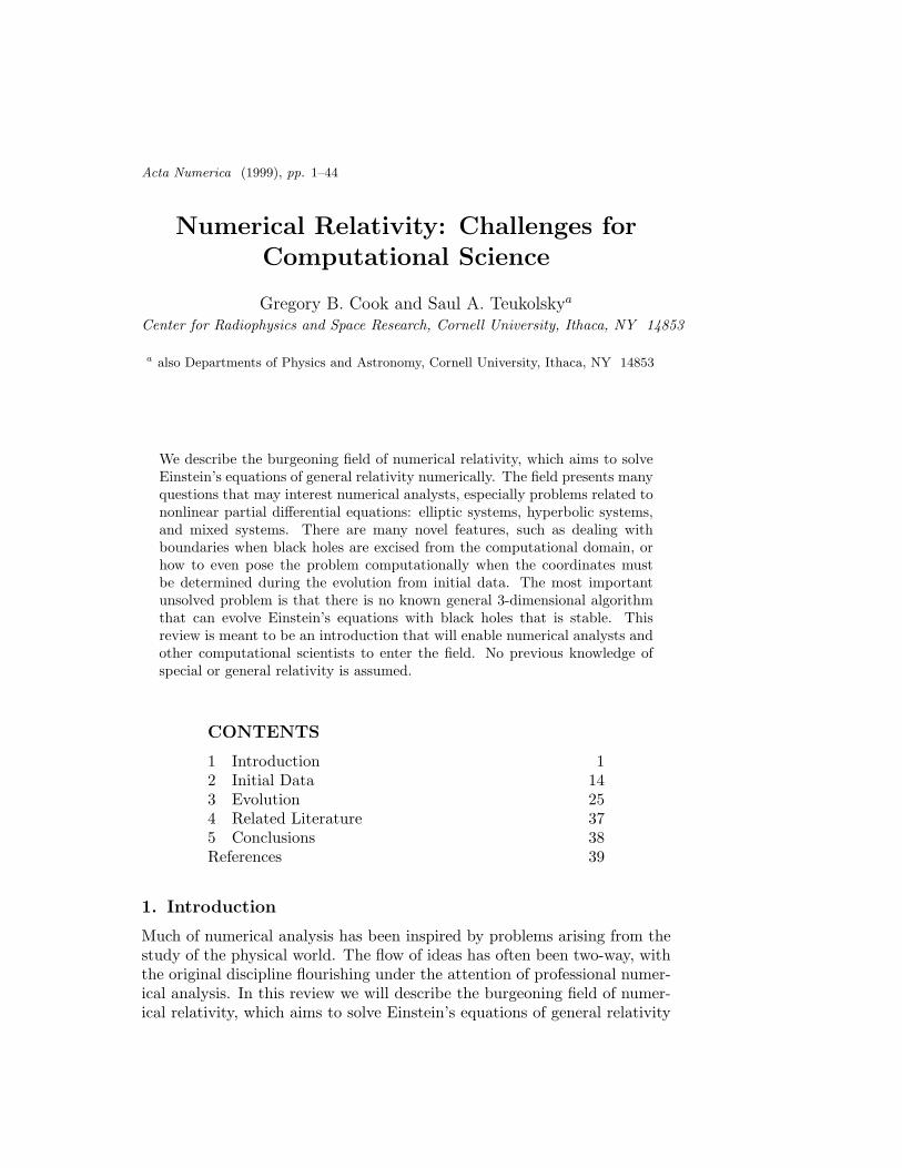
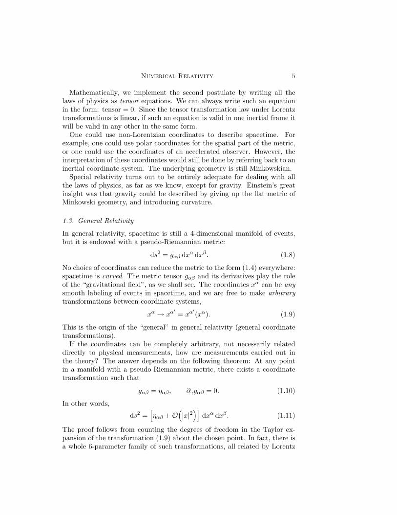
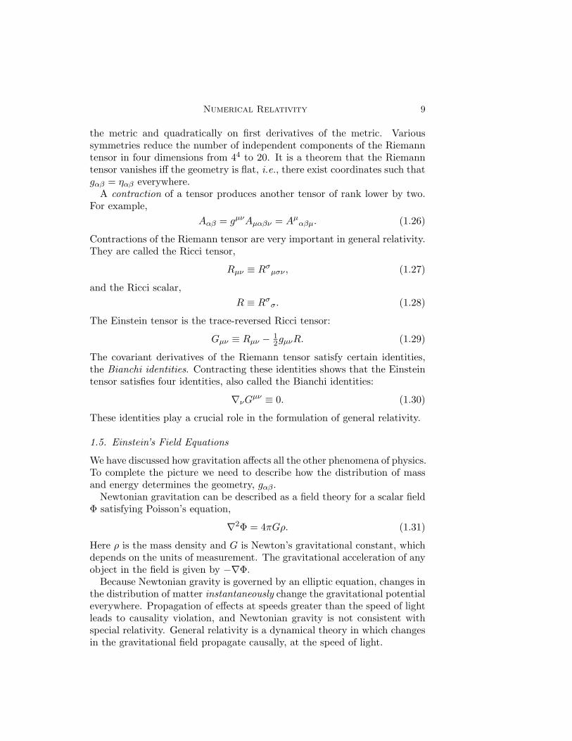
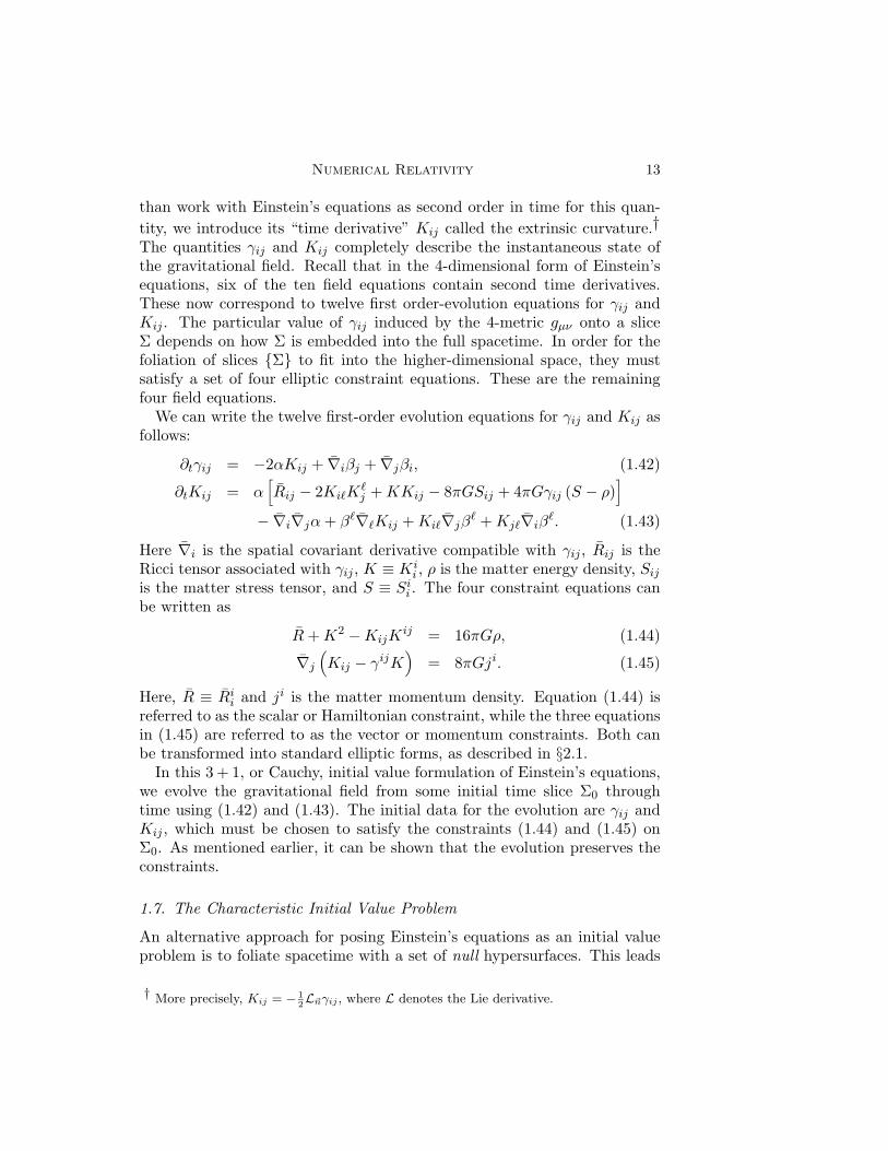
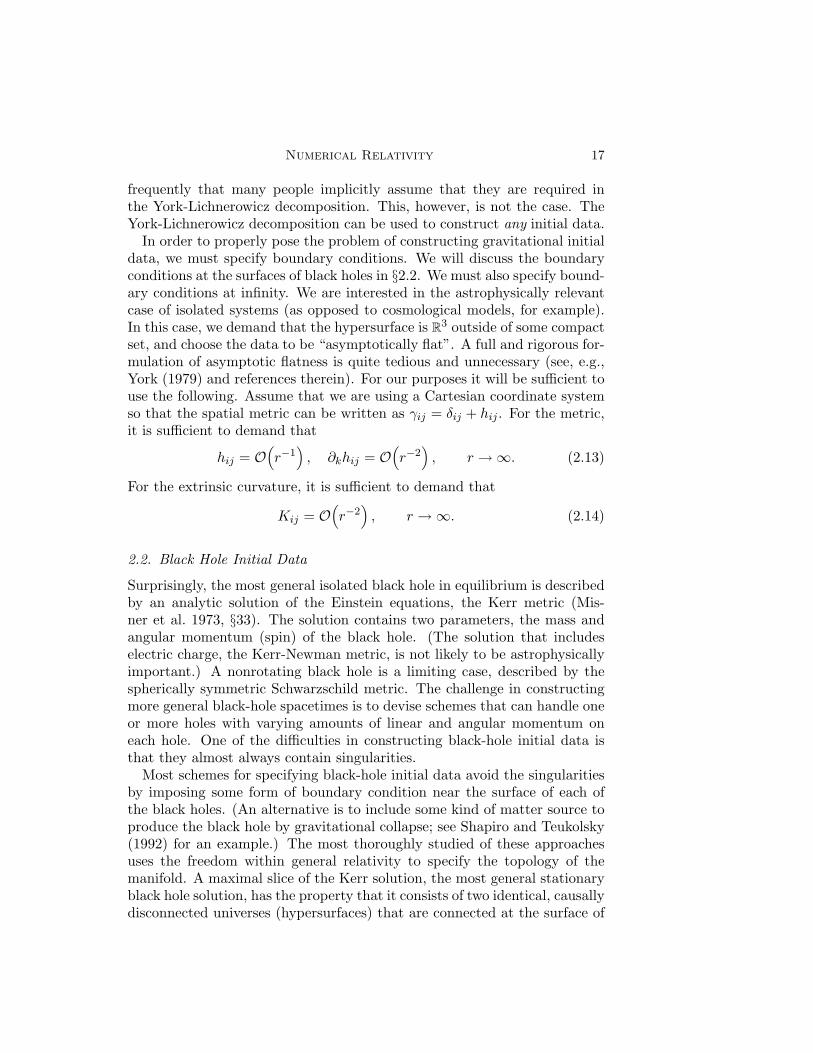
Fig. 1. The 3 + 1 decomposition of spacetime. Neighboring slices of the foliationare labeled by the value of the time coordinate on that slice. Spatial coordinatesremain constant along the ~t direction as they evolve from Σt0 to Σt0+dt. ~n is the
unit normal vector to the slice Σt0 .
Now in general one is not required to evolve initial data off the t = 0 slicealong the normal congruence. Consider a non-normal congruence threadingthe family of spacelike hypersurfaces. Let
~t =∂
∂t(1.37)
be the tangent vector to the congruence, i.e., ~t connects points with thesame spatial coordinates xi.
Then we can write (see Fig. 1)
~t = α~n+ ~β, ~β · ~n = 0. (1.38)
The spatial vector βi is called the shift vector (sometimes denoted N i in theliterature). In terms of the metric components, equation (1.38) is equivalentto
gtt =∂
∂t· ∂∂t
= −α2 + βiβi, (1.39)
gti =∂
∂t· ∂∂xi
= βi. (1.40)
Denote the spatial part of the metric gij by γij . The quantity γij describesthe intrinsic geometry on a 3-dimensional slice Σ. Then in light of equa-tions (1.39) and (1.40), the general pseudo-Riemannian metric (1.8) can berewritten as
ds2 = −α2 dt2 + γij( dxi + βi dt)( dxj + βj dt). (1.41)
This is the standard starting point of most numerical attempts to solveEinstein’s equations.
We have seen that the four coordinate degrees of freedom in the theoryare parametrized by α and βi. (This is also called the gauge freedom of thetheory.) We regard γij as a “fundamental” variable of the theory. Rather
Numerical Relativity 13
than work with Einstein’s equations as second order in time for this quan-tity, we introduce its “time derivative” Kij called the extrinsic curvature.†The quantities γij and Kij completely describe the instantaneous state ofthe gravitational field. Recall that in the 4-dimensional form of Einstein’sequations, six of the ten field equations contain second time derivatives.These now correspond to twelve first order-evolution equations for γij andKij . The particular value of γij induced by the 4-metric gµν onto a sliceΣ depends on how Σ is embedded into the full spacetime. In order for thefoliation of slices Σ to fit into the higher-dimensional space, they mustsatisfy a set of four elliptic constraint equations. These are the remainingfour field equations.
We can write the twelve first-order evolution equations for γij and Kij asfollows:
∂tγij = −2αKij + ∇iβj + ∇jβi, (1.42)
∂tKij = α[Rij − 2Ki`K
`j +KKij − 8πGSij + 4πGγij (S − ρ)
]− ∇i∇jα+ β`∇`Kij +Ki`∇jβ` +Kj`∇iβ`. (1.43)
Here ∇i is the spatial covariant derivative compatible with γij , Rij is theRicci tensor associated with γij , K ≡ Ki
i , ρ is the matter energy density, Sijis the matter stress tensor, and S ≡ Sii . The four constraint equations canbe written as
R+K2 −KijKij = 16πGρ, (1.44)
∇j(Kij − γijK
)= 8πGji. (1.45)
Here, R ≡ Rii and ji is the matter momentum density. Equation (1.44) isreferred to as the scalar or Hamiltonian constraint, while the three equationsin (1.45) are referred to as the vector or momentum constraints. Both canbe transformed into standard elliptic forms, as described in §2.1.
In this 3 + 1, or Cauchy, initial value formulation of Einstein’s equations,we evolve the gravitational field from some initial time slice Σ0 throughtime using (1.42) and (1.43). The initial data for the evolution are γij andKij , which must be chosen to satisfy the constraints (1.44) and (1.45) onΣ0. As mentioned earlier, it can be shown that the evolution preserves theconstraints.
1.7. The Characteristic Initial Value Problem
An alternative approach for posing Einstein’s equations as an initial valueproblem is to foliate spacetime with a set of null hypersurfaces. This leads
† More precisely, Kij = − 12L~nγij , where L denotes the Lie derivative.
14 Cook and Teukolsky
to the 2 + 2, or characteristic, initial value formulation of general relativity(see Bishop, Gomez, Lehner, Maharaj and Winicour (1997b) and referencestherein). The characteristic formulation of Einstein’s equations is particu-larly adept at following gravitational waves propagating through the space-time, but has difficulty in highly dynamic, strong field regions where thenull surfaces tend to form caustics. Because of this problem, and the lim-ited scope of this review, we will focus entirely on the Cauchy initial valueformulation of general relativity.
2. Initial Data
The initial data for the Cauchy formulation of general relativity are themetric γij and extrinsic curvature Kij . These each have six componentsthat must be fixed, a total of twelve. As discussed in §1.6, general rela-tivity has a 4-dimensional coordinate invariance or gauge freedom that canbe parametrized by the lapse and shift functions. These functions can bechosen to specify four of the twelve quantities (or relations among them).The four constraint equations fix four more quantities. The remaining fourquantities describe the two “dynamical degrees of freedom” of general rel-ativity, four quantities satisfying first-order dynamical equations, or equiv-alently two quantities satisfying second-order wave-like equations. Thesefour quantities are freely specifiable initial data, corresponding roughly tothe initial gravitational wave content of the spacetime.
In the weak field limit where the equations of general relativity can belinearized, there are clear ways to determine which components are dynamic,which are constrained, and which are gauge. However, in the full nonlineartheory, there is no unique decomposition. The approach one follows fordecomposing the metric and extrinsic curvature determines the final formof the elliptic equations that constrain the initial data.
2.1. York-Lichnerowicz conformal decomposition
The most widely used approach for separating out the freely specifiableinitial data from the constrained initial data is the York-Lichnerowicz con-formal decomposition. Here we give a brief summary. For a more completediscussion, with references to the original literature, see York (1979).
First the metric is decomposed into a conformal factor multiplying a 3-metric:
γij ≡ ψ4γij . (2.1)
The auxiliary 3-metric γij is called the conformal 3-metric. Its determinantcan be normalized to some convenient value, leaving five degrees of freedom.Using (2.1), we can rewrite the Hamiltonian constraint (1.44) as
∇2ψ − 18ψR−
18ψ
5K2 + 18ψ
5KijKij = −2πGψ5ρ, (2.2)
Numerical Relativity 15
where ∇2 and R are the scalar Laplace operator and the Ricci scalar asso-ciated with γij . Equation (2.2) shows that ψ is constrained by the ellipticHamiltonian constraint. The five components of γij contain two freely speci-fiable degrees of freedom together with three pieces of information related tothe 3-dimensional spatial gauge freedom. These three pieces of informationare essentially the initial choice of the spatial coordinate system which arethen propagated by the shift vector.
The extrinsic curvature is decomposed into its trace K and trace-free partsAij via
Kij ≡ Aij + 13γ
ijK. (2.3)
The embedding of the initial data hypersurface within the full spacetimefixes the initial time coordinate, the choice then being propagated by thelapse. Thus one piece of Kij is used to specify the time coordinate, and it istaken to be the trace K for geometric and physical reasons (O Murchadhaand York 1974). K is thus freely specifiable in the initial data. The fivecomponents of Aij can be further decomposed using a transverse-tracelessdecomposition. In order to write the full set of constraints in terms ofoperators on the conformal 3-geometry, it is necessary to also conformallydecompose Aij . The conformal and transverse-traceless decompositions ofAij do not commute, leading to two different formulations of the full set ofconstraint equations. Historically, the most widely used decomposition hasapplied the transverse-traceless decomposition to the conformally rescaledversion of Aij . While somewhat less physically motivated, under certain sim-plifying assumptions this approach decouples the vector constraint equation(1.45) from the Hamiltonian constraint. This was an important simplifica-tion when computational power was limited. This is not so much of a con-cern any more and we present the alternative decomposition here. Readerswishing to skip the details can proceed to equation (2.9).
We first decompose Aij as
Aij ≡ (LW )ij +Qij , (2.4)
where
(LW )ij ≡ γi`∇`W j + γj`∇`W i − 23γ
ij∇`W ` (2.5)
and Qij is a symmetric transverse-traceless tensor (i.e., it satisfies ∇jQij =Qii = 0). The remainder of Aij , constructed from (LW )ij , is referred to asthe trace-free longitudinal part of the extrinsic curvature.
In general, one would construct Qij from a general symmetric, trace-freetensor M ij by subtracting off its longitudinal part. However, since the vectorconstraint is linear in Kij , we can rewrite (2.4) as
Aij ≡ ψ−4(LV )ij + ψ−10M ij , (2.6)
16 Cook and Teukolsky
where (LV )ij is defined as in (2.5) but with ∇i → ∇i and γij → γij . Notethat the longitudinal part of Aij is constructed from a new vector V i, notW i (see below), and M ij ≡ ψ10M ij . We can now rewrite the vector, ormomentum constraint (1.45) as
∆LVi + 6(LV )ij∇j lnψ = 2
3 γij∇jK − ψ−6∇jM ij + 8πGψ4ji. (2.7)
This is a vector elliptic equation for V i, where
∆LVi ≡ ∇j(LV )ij = γj`∇j∇`V i + 1
3 γi`∇`(∇jV j) + γi`R`jV
j , (2.8)
and Rij is the Ricci tensor associated with the conformal 3-geometry γij .The vector V i is a linear combination of both the three constrained lon-gitudinal components of Aij represented by W i in (2.4) and the longitu-dinal components of M ij . Since Aij is traceless, this means that Qij , thetransverse-traceless part of M ij , contains two freely specifiable quantitiesthat are taken as the two gravitational degrees of freedom.
Finally, given (2.6), we can rewrite the Hamiltonian constraint (2.2) as
∇2ψ − 18ψR−
112ψ
5K2 + 18ψ
5γij γ`m(LV )i`(LV )jm (2.9)
+14ψ−1γij γ`m(LV )i`M jm + 1
8ψ−7γij γ`mM
i`M jm = −2πGψ5ρ.
Equations (2.9) and (2.7) form the coupled set of four elliptic equations thatmust be solved with appropriate boundary conditions in order to properlyspecify gravitational data on a given constant-time slice.
In the historically more widely used decomposition, the trace-free extrinsiccurvature is expressed as
Aij = ψ−10Aij ≡ ψ−10[(LV )ij + M ij
], (2.10)
and the Hamiltonian and momentum constraints reduce to
∇2ψ − 18ψR−
112ψ
5K2 + 18ψ−7γij γ`mA
i`Ajm = −2πGψ5ρ, (2.11)
∆LVi = 2
3ψ6γij∇jK − ∇jM ij + 8πGψ10ji. (2.12)
For more on this version of the decomposition, see York (1979).Two simplifying (but restrictive) choices are frequently made with the
York-Lichnerowicz decomposition. First, the conformal 3-metric γij is takento be flat (i.e, δij in Cartesian coordinates) and the full 3-geometry is saidto be conformally flat. This is a reasonable choice, since it is true in thelimit of weak gravity. This assumption simplifies the elliptic equations be-cause now Rij = R = 0 and the derivative operators become the familiarflat-space operators. The second assumption usually made is that K = 0.This says that the initial data slice Σ0 is maximally embedded in the fullspacetime. This is a physically reasonable assumption and, for the case ofthe decomposition (2.10), decouples the Hamiltonian and momentum con-straint equations (2.11) and (2.12). These simplifying choices are used so
Numerical Relativity 17
frequently that many people implicitly assume that they are required inthe York-Lichnerowicz decomposition. This, however, is not the case. TheYork-Lichnerowicz decomposition can be used to construct any initial data.
In order to properly pose the problem of constructing gravitational initialdata, we must specify boundary conditions. We will discuss the boundaryconditions at the surfaces of black holes in §2.2. We must also specify bound-ary conditions at infinity. We are interested in the astrophysically relevantcase of isolated systems (as opposed to cosmological models, for example).In this case, we demand that the hypersurface is R3 outside of some compactset, and choose the data to be “asymptotically flat”. A full and rigorous for-mulation of asymptotic flatness is quite tedious and unnecessary (see, e.g.,York (1979) and references therein). For our purposes it will be sufficient touse the following. Assume that we are using a Cartesian coordinate systemso that the spatial metric can be written as γij = δij + hij . For the metric,it is sufficient to demand that
hij = O(r−1
), ∂khij = O
(r−2
), r →∞. (2.13)
For the extrinsic curvature, it is sufficient to demand that
Kij = O(r−2
), r →∞. (2.14)
2.2. Black Hole Initial Data
Surprisingly, the most general isolated black hole in equilibrium is describedby an analytic solution of the Einstein equations, the Kerr metric (Mis-ner et al. 1973, §33). The solution contains two parameters, the mass andangular momentum (spin) of the black hole. (The solution that includeselectric charge, the Kerr-Newman metric, is not likely to be astrophysicallyimportant.) A nonrotating black hole is a limiting case, described by thespherically symmetric Schwarzschild metric. The challenge in constructingmore general black-hole spacetimes is to devise schemes that can handle oneor more holes with varying amounts of linear and angular momentum oneach hole. One of the difficulties in constructing black-hole initial data isthat they almost always contain singularities.
Most schemes for specifying black-hole initial data avoid the singularitiesby imposing some form of boundary condition near the surface of each ofthe black holes. (An alternative is to include some kind of matter source toproduce the black hole by gravitational collapse; see Shapiro and Teukolsky(1992) for an example.) The most thoroughly studied of these approachesuses the freedom within general relativity to specify the topology of themanifold. A maximal slice of the Kerr solution, the most general stationaryblack hole solution, has the property that it consists of two identical, causallydisconnected universes (hypersurfaces) that are connected at the surface of
18 Cook and Teukolsky
the black hole by an “Einstein-Rosen bridge” (Einstein and Rosen 1935,Misner et al. 1973, Brandt and Seidel 1995). We are free to demand thatmore general black-hole initial data be constructed in a similar way from twoidentical hypersurfaces joined at the black hole “throats” (Misner 1963). Amethod of images applicable to tensors can be used to enforce the isometrybetween the solutions on the two hypersurfaces and the isometry inducesboundary conditions on the topologically S2 fixed point sets that form theboundaries where the two hypersurfaces are joined (Bowen 1979, Bowen andYork 1980, Kulkarni, Shepley and York 1983, Kulkarni 1984).
A second approach completely bypasses the issue of the topology of theinitial data hypersurface by imposing a boundary condition at the “apparenthorizon” associated with each black hole (Thornburg 1987). We will comeback to apparent horizons in §3.3.
Yet another approach is based on factoring out the singular behavior of theinitial data (Brandt and Brugmann 1997). This approach uses an alternativetopology for the initial data hypersurface in which each black hole in “our”universe is connected to a black hole in a separate universe, producing asolution with NBH + 1 causally disconnected universes joined at the throatsof NBH black holes. This approach has the advantage of not requiring thatboundary conditions be imposed on a spherical surface at each hole, makingit easier to use a Cartesian coordinate system.
All three of these approaches for constructing black-hole initial data aresimplified by being constructed on a conformally flat, maximally embed-ded hypersurface. Because they all use the alternative transverse-tracelessdecomposition of the extrinsic curvature, the Hamiltonian and momentumconstraint equations are decoupled. In vacuum, there exists an analytic solu-tion for the background extrinsic curvature Aij that satisfies the momentumconstraint (1.45) for any ψ (Bowen and York 1980). For a single black hole,this solution is
Aij =3G2r2
[P inj + P jni − (f ij − ninj)P `n`
]+
3Gr3
[εki`S`nkn
j + εkj`S`nkni]. (2.15)
Here P i and Si are the linear and angular momenta of the black hole, r isthe Cartesian coordinate radius from the center of the black hole locatedat Ci, and ni ≡ (xi − Ci)/r in Cartesian coordinates. fij is the flat metricin whatever coordinate system is used, and εijk is the totally antisymmetrictensor. For a general spatial metric γij , it is defined as εijk ≡
√γ[ijk], where
[ijk] is the totally antisymmetric permutation symbol with [123] = 1, andγ = det γij . The solution (2.15) is constructed as in (2.10) with M ij = 0and can be verified easily by noting that the momentum constraint (2.12)reduces under the assumptions above to ∇jAij = 0. Solutions for multiple
Numerical Relativity 19
black holes, each with a different center, can be constructed as a linearsuperposition. As given, (2.15) will not satisfy the isometry condition whenthe topology is chosen to be two identical hypersurfaces. However, this canbe corrected by adding an infinite series of correction terms; see Cook (1991)for references and an explicit algorithm for computing the series.‡
With an analytic solution for Aij , only a single, quasi-linear elliptic equa-tion for ψ needs to be solved to obtain the complete initial data. Equation(2.11) reduces to
∇2ψ +18ψ−7γij γ`mA
i`Ajm = 0, (2.16)
The boundary condition on ψ at large distances from the collection of blackholes can be obtained from its asymptotic behavior, ψ → 1 +C/r+O
(r−2
)where C is a constant. When the choice of topology is that of two isometrichypersurfaces, the isometry induces a boundary condition on the sphericalsurface where the two hypersurfaces connect,
ni∇iψ = − ψ2r. (2.17)
When the inner boundary is constructed to be an apparent horizon insteadof using two isometric hypersurfaces, (2.17) is modified with a nonlinearcorrection; see Thornburg (1987) for details.
The limitation of all three of the solution schemes described above is thatthe simplifying choice of a conformally flat 3-geometry and the analytic so-lution for the background extrinsic curvature represent a very limited choicefor the unconstrained, dynamical portion of the gravitational fields. Also, amaximal slice (K = 0) may not always be a good choice for numerical evo-lutions. Moving beyond these limitations is the major challenge to be facedin constructing black-hole initial data. This will certainly require solvingthe full coupled system of equations, (2.9) and (2.7) (or alternatively (2.11)and (2.12)).
2.3. Equilibrium Stars
An equilibrium or stationary solution of Einstein’s equations has no timedependence. In coordinate-invariant language, the solution admits a Killingvector that is timelike at infinity. The metric is specified by a solution ofthe initial value equations that also satisfies the dynamical equations withtime derivatives set to zero. An important class of such solutions describesrotating equilibrium stars, which are axisymmetric. In axisymmetry thereare just three nontrivial initial value equations. There is only one furtherequation to be satisfied from among the dynamical equations, and it is also
‡ In equation (B7) of Cook (1991), “1 for n = 1” should read “α−1 for n = 1”.
20 Cook and Teukolsky
elliptic because the time derivatives have been set to zero. It is simpler inthis case just to choose an appropriate form for the metric and solve theresulting four equations directly, without going through something like theYork-Lichnerowicz decomposition. There are many numerical approachesfor solving these equations to high accuracy (see Butterworth and Ipser(1976) and Friedman, Ipser and Parker (1986) and references therein for adescription of a pseudo-spectral method; Komatsu, Eriguchi and Hachisu(1989) and Cook, Shapiro and Teukolsky (1994) and references therein foran iterative method based on a Green’s function; Bonazzola, Gourgoulhon,Salgado and Marck (1993) and references therein for a spectral method).
2.4. Binary Black Holes
The most important computations confronting numerical relativity involvebinary systems containing black holes or neutron stars. Large experimentalfacilities are being built around the world in an effort to detect gravitationalwaves directly from astrophysical sources in the next few years (Abramoviciet al. 1992). These binary systems are prime candidates as sources: as theyemit gravitational waves they lose energy and slowly spiral inwards, untilthey finally plunge together emitting a burst of radiation.
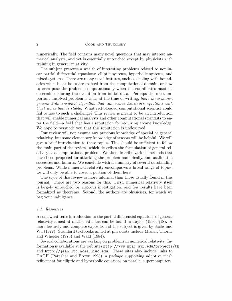
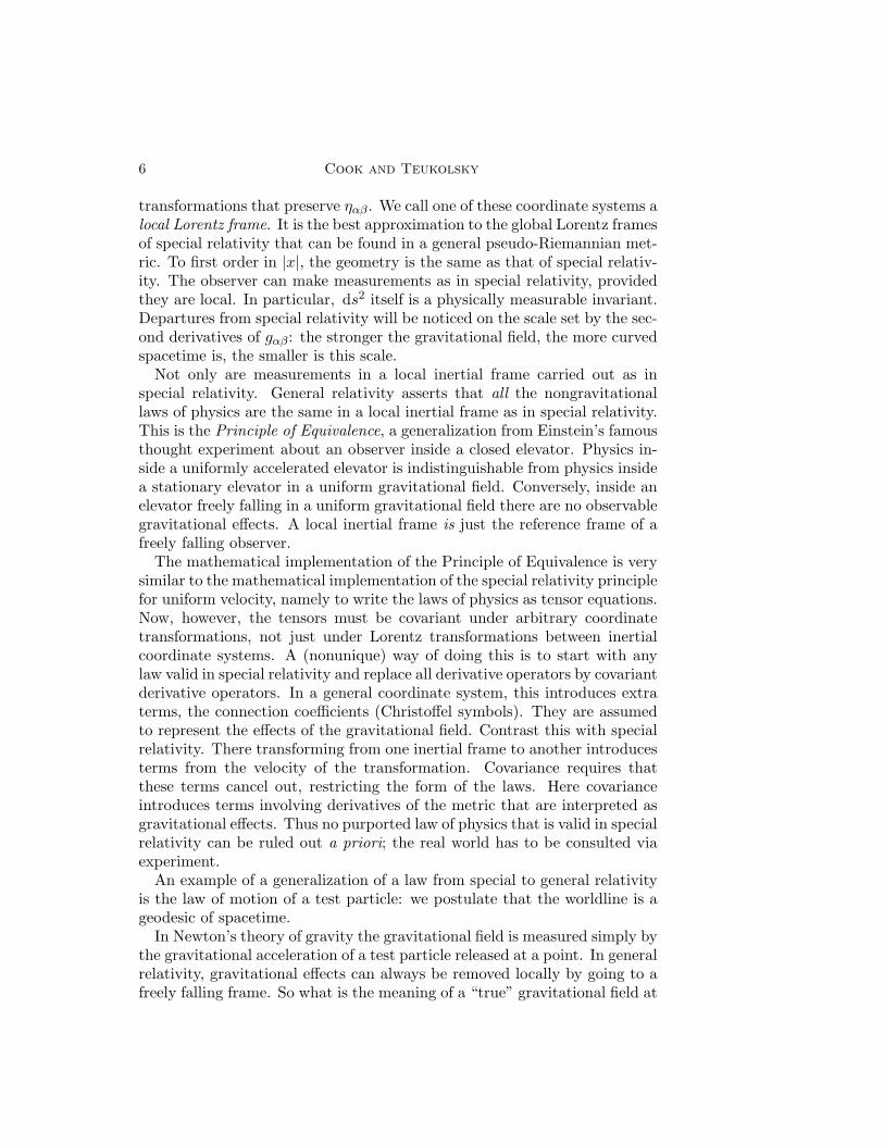
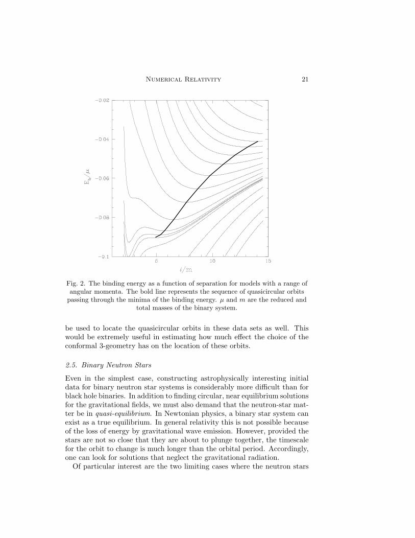
Since emission of gravitational radiation tends to circularize elliptical or-bits, one is interested in initial data corresponding to quasicircular orbits.For the case of a binary black hole system, a very high accuracy survey hasbeen performed to locate these orbits (Cook 1994). In this work, quasicircu-lar orbits were found by locating binding energy minima§ along sequencesof models with constant angular momentum (see Fig. 2). Locating theseminima required extremely high accuracy, which was achieved using a com-bination of techniques. First, the Hamiltonian constraint (2.16) was dis-cretized on a numerically generated coordinate system specifically adaptedto the problem, then solved using a FAS/block-multigrid algorithm (Cooket al. 1993). Then the results of several runs at different resolutions werecombined using Richardson extrapolation to obtain results accurate to onepart in 105.
There are efforts under way to produce binary black hole initial data thatmay be more astrophysically realistic by using a linear combination of singlespinning black hole solutions to provide a conformal 3-geometry γij thatis not flat (Matzner, Huq and Shoemaker 1998). If the constraints can besuccessfully solved on this non-flat background, then a similar procedure can
§ The equations for equilibrium stars can be derived from an energy variational principle.Thus the stability of such stars can be analyzed by examining turning points along one-parameter sequences of equilibrium solutions (Sorkin 1982). The extension of this ideato quasi-equilibrium sequences is plausible, but has not been rigorously demonstrated.
Numerical Relativity 21
Fig. 2. The binding energy as a function of separation for models with a range ofangular momenta. The bold line represents the sequence of quasicircular orbits
passing through the minima of the binding energy. µ and m are the reduced andtotal masses of the binary system.
be used to locate the quasicircular orbits in these data sets as well. Thiswould be extremely useful in estimating how much effect the choice of theconformal 3-geometry has on the location of these orbits.
2.5. Binary Neutron Stars
Even in the simplest case, constructing astrophysically interesting initialdata for binary neutron star systems is considerably more difficult than forblack hole binaries. In addition to finding circular, near equilibrium solutionsfor the gravitational fields, we must also demand that the neutron-star mat-ter be in quasi-equilibrium. In Newtonian physics, a binary star system canexist as a true equilibrium. In general relativity this is not possible becauseof the loss of energy by gravitational wave emission. However, provided thestars are not so close that they are about to plunge together, the timescalefor the orbit to change is much longer than the orbital period. Accordingly,one can look for solutions that neglect the gravitational radiation.
Of particular interest are the two limiting cases where the neutron stars
22 Cook and Teukolsky
are co-rotating (no rotation in the frame co-rotating with the binary system)and counter-rotating (no rotation in the rest frame of the center of mass).Several schemes have been devised to construct initial data for a neutron-star binary in quasi-equilibrium (Wilson, Mathews and Marronetti 1996,Bonazzola, Gourgoulhon and Marck 1997, Baumgarte, Cook, Scheel, Shapiroand Teukolsky 1998). All of these schemes are based on the simplifyingassumptions of conformal flatness and maximal slicing, differing primarilyin how the neutron star matter is handled. We give here one particularexample of the system of equations to be solved. First, the gravitationalfield equations are (Wilson et al. 1996)
Aij =ψ−4
2α(Lω)ij , (2.18)
∇2ωi +13f i`∇`∇jωj = 2ψ10Aij∇j
(αψ−6
)+ 16πGαψ4ji, (2.19)
∇2ψ = −18ψ
5fijf`m(ψ4Ai`)(ψ4Ajm)− 2πGψ5ρ, (2.20)
∇2(αψ) = (αψ)[
78ψ
4fijf`m(ψ4Ai`)(ψ4Ajm)
+ 2πGψ4(ρ+ 2S)]. (2.21)
The spatial metric is decomposed as in (2.1) and is taken to be conformallyflat γij = fij (i.e., fij = δij in Cartesian coordinates). We assume maximalslicing (K = 0), and get the equation for the trace-free extrinsic curvature(2.18) from physical arguments for quasi-equilibrium. Note that (2.18) isvery similar to the (2.6) except that M ij is not present and we divide by2α. We obtain equation (2.19) by substituting (2.18) into the momentumconstraint (1.45). Note that the principal part of the operator for (2.19) isthe same as in (2.7). The conformal factor ψ is fixed via the Hamiltonianconstraint which now takes the form in (2.20). Finally, the lapse α is fixedvia (2.21) which enforces the maximal slicing condition on neighboring slices.
For the counter-rotating case, the fluid velocity is irrotational (curl-free),and can be derived from a scalar velocity potential even in general relativity(Teukolsky 1998, Shibata 1998). The matter equations are
1ψ2√f
∂
∂xi
(f ijψ2
√f∂ϕ
∂xj
)= βi∇i
(λ
α2
)(2.22)
−(ψ−4f ij∇jϕ−
λ
α2βi)∇i ln
(αnB
h
),
λ ≡ C+ βi∇iϕ = α[h2 + ψ−4f ij(∇iϕ)∇jϕ
]1/2, (2.23)
h2 ≡ −ψ−4f ij(∇iϕ)∇jϕ+1α2
(C + βi∇iϕ
)2, (2.24)
βi ≡ ωi + Ωξi, (2.25)
Numerical Relativity 23
where ϕ is the velocity potential and C is an integration constant. Ω is aconstant specifying the angular velocity of the rotating binary system andξi is a circular rotation vector ( ξi = (−y, x, 0) in Cartesian coordinates forrotation about the z axis). nB is the baryon number density (see (2.31)below). The domain of solution for (2.22) is the volume covered by matterand the solution must satisfy(
ψ−4f ij∇jϕ−λ
α2βi)∇inB
∣∣∣∣surf
= 0 (2.26)
at the boundary of the matter where nB goes to zero.Finally, the matter equations couple back into the gravitational field equa-
tions through the source terms on the right-hand-sides of (2.19), (2.20), and(2.21), defined by
ρ = (ρ0 + ρi + P )1
α2h2
(C + βi∇iϕ
)2− P, (2.27)
S = (ρ0 + ρi + P )ψ−4
h2f ij(∇iϕ)∇jϕ+ 3P, (2.28)
ji = (ρ0 + ρi + P )ψ−4
αh2
(C + β`∇`ϕ
)f ij∇jϕ, (2.29)
h ≡ ρ0 + ρi + P
ρ0, (2.30)
ρ0 ≡ mBnB, (2.31)
where ρ0, ρi, and P are, respectively, the rest mass density, internal energydensity, and pressure of the matter in the matter’s rest frame. These areall determined from the enthalpy h via (2.30) given nB, the baryon massdensity mB, and an equation of state for the matter.
We find then, that solving for an irrotational neutron-star binary systemin quasi-equilibrium requires the solution of a set of six coupled, nonlinearelliptic equations given by (2.19), (2.20), (2.21), and (2.22). The solutiondepends on two free parameters, C and Ω, which must be chosen to allowa self-consistent solution. A scheme for doing this could be based on thealgorithm described by Baumgarte et al. (1998) for the slightly simpler caseof a synchronous (co-rotating) binary system. A stable iterative schemeis obtained by rescaling the equations so that the outermost point on thesurface of each neutron star, where it crosses the axis connecting the twostars, is at a fixed coordinate location. The innermost point on the surfaceof each star is taken as an input parameter for a particular solution androughly corresponds to the free parameter Ω. Next, the maximum value ofthe density ρ0 is taken as another input parameter, roughly correspondingto C. The exact values of Ω and C are obtained at each step of the iterationby solving a set of nonlinear algebraic equations that follow from equation(2.24). What complicates the solution of these six equations is that, while
24 Cook and Teukolsky
five of them are solved on a domain extending out to radial infinity, (2.22)must be solved on the limited domain consisting of the volume containingmatter. The boundary of this volume is not prescribed, but is determinedby the solution. The first set of successful solutions to the equations for irro-tational binaries has been obtained by Bonazzola, Gourgoulhon and Marck(1999) using spectral methods.
2.6. Summary
Common to all of these current efforts at constructing initial data is theneed to solve a large set of coupled nonlinear elliptic equations with com-plicated boundaries over a large range of length scales. The classic problemof constructing axisymmetric rotating neutron-star models has been studiedextensively, and highly sophisticated and efficient computational techniquesare now commonly used. The situation is not nearly so well in hand forthe other examples described above. These problems are ripe for new ideasand algorithms. They have been attacked principally using finite differencetechniques, although Bonazzola, Gourgoulhon and Marck (1998) are explor-ing spectral techniques for neutron-star binaries, and Arnold, Mukherjeeand Pouly (1998) have applied finite element techniques to the problem ofsolving the Hamiltonian constraint. Which numerical schemes will work thebest is still an open question. A good scheme must balance efficiency andspeed against accuracy. It must be able to resolve the different length scalesof the problem, even though the fields vary on characteristic length scalescomparable to the radius of the star when near to the star, while the outerboundary conditions must be imposed at large distances from the stars.
There is a great need for both efficiency and accuracy. Physicists areinterested in performing extensive parameter space surveys in order to un-derstand the physical content of the initial data. With sufficient accuracy,such surveys can also provide great insight into dynamical, but slowly evolv-ing configurations (the quasi-equilibrium approximation). The accuracy ofsolutions is limited not only by the truncation error of the numerical schemeand the grid resolutions used, but also by the approximations made. Ideally,the outer boundary should extend to infinity, but this often poses problemsnumerically. In practice, the outer boundary is usually approximated via afalloff condition at large radius (cf. equations (2.13) and (2.14)). How farout this radius can be pushed while still maintaining accuracy near the starsdepends on the numerical scheme and gridding choices.
There are many other issues that must be addressed. Perhaps the mostimportant, besides efficiency and accuracy, are: How does the nonlinearityof the coupled system affect the choice of the solution scheme? And williterative schemes for solving the coupled system remain stable when thenonlinear couplings become strong?
Numerical Relativity 25
3. Evolution
3.1. Standard ADM Form
In its simplest form, evolving Einstein’s equations as a Cauchy problem in-volves updating the metric γij and extrinsic curvature Kij using the evolu-tion equations (1.42) and (1.43). A pure evolution scheme solves only suchtime evolution equations. It relies on the evolution equations to preservethe validity of the constraints computationally as well as analytically. It isalso possible to determine some of the dynamical quantities from evolutionequations and others from the constraint equations at each time step. Suchalgorithms are expected to be less efficient than pure evolution schemes,since they require the solution of elliptic equations for the constraints ateach time step. These mixed strategies have been the preferred algorithmsin 1- and 2-dimensional problems, because of difficulties in designing stable,accurate pure evolution schemes. Moreover, as mentioned earlier, there isno known general 3-dimensional algorithm that can evolve Einstein’s equa-tions with black holes that is stable. While we will emphasize pure evolutionschemes in this review, one should bear in mind the possibility that some ex-plicit enforcement of the constraints may be necessary to guarantee a stablealgorithm.
As discussed in §1.6, when solving equations (1.42) and (1.43), we mustseparately specify exactly how far along we are evolving each point in propertime (physical time) by specifying the lapse function α. We must also choosehow the spatial coordinates labeling a particular point on the hypersurfacewill change by specifying the shift vector βi. Assume that we have fixedthese four kinematical quantities somehow, and that we are in vacuum sothat the matter terms vanish. Then, if we express the tensors in terms ofa coordinate basis, we can write the evolution equations (1.42) and (1.43)explicitly as
∂tγij − β`∂`γij = γ`j∂iβ` + γi`∂jβ
` − 2αKij , (3.1)
∂tKij − β`∂`Kij = Ki`∂jβ` +Kj`∂iβ
` − 2αKi`K`j + αKKij
− 12αγ
`m∂`∂mγij + ∂i∂jγ`m − ∂i∂`γmj − ∂j∂`γmi
+ γnp[(∂iγjn + ∂jγin − ∂nγij)∂`γmp
+ (∂`γin)∂pγjm − (∂`γin)∂mγjp]
− 12γ
np[(∂iγjn + ∂jγin − ∂nγij)∂pγ`m + (∂iγ`n)∂jγmp
]− ∂i∂jα+ 1
2γ`m (∂iγjm + ∂jγim − ∂mγij) ∂`α. (3.2)
Notice that (3.1) and (3.2) do not form a simple wave equation. In fact,(3.1) contains no derivatives of Kij at all, while (3.2) contains both linear
26 Cook and Teukolsky
combinations of second derivatives of γij and quadratic combinations offirst derivatives of γij . We call the set of evolution equations given by (3.1)and (3.2) the “standard ADM form”.¶ The “non-Laplacian” like secondderivatives in equation (3.2) can be removed by certain modifications to thestandard ADM equations (see Baumgarte and Shapiro (1999) and referencewithin), resulting in a system that seems to be better behaved.
In general, the ADM equations are not of any known mathematical type.In particular, they do not satisfy any of the standard definitions of hyper-bolicity. While physical effects propagate at the speed of light in generalrelativity, γij and Kij are not simple physical quantities. Rather, they aregauge-dependent quantities whose values depend on the choice of the lapseα and shift βi. These can be chosen to allow for propagation of waves in γijand Kij at arbitrary speeds.
3.2. Hyperbolic Forms
There is a long history of analytic studies of hyperbolic formulations of gen-eral relativity (Foures-Bruhat 1952, Fischer and Marsden 1972, Friedrich1985); see also (Taylor 1996, §18.8). The earliest approaches made specialgauge choices to rewrite (3.1) and (3.2) in the form of a manifestly sym-metric hyperbolic system (Foures-Bruhat 1952, Fischer and Marsden 1972).Interest in using such formulations in numerical studies has been relativelyrecent (Bona and Masso 1992). The initial motivation for exploring thesetechniques was to put Einstein’s equations into a form that could makemore direct use of the vast repertoire of numerical techniques for handlingfirst-order symmetric hyperbolic systems such as the equations of fluid me-chanics. It was soon realized, however, that a clear understanding of thecharacteristic speeds of propagation of the evolving variables was also quiteuseful. This is especially true for the problem of evolving spacetimes thatcontain black holes, as discussed below. It is also hoped that having theequations in a form that can be more readily analyzed will aid, for exam-ple, in properly posing boundary conditions or in treating the propagationof errors in the constraints (Frittelli 1997, Brodbeck, Frittelli, Hubner andRuela 1998). In particular, it is hoped that stable evolution schemes can bedeveloped that do not require that elliptic constraint equations be solved oneach time step (Scheel, Baumgarte, Cook, Shapiro and Teukolsky 1998).
A potential problem with using the gauge freedom to achieve explicitly hy-perbolic forms is that it is widely believed that successful numerical schemeswill need to exploit the gauge freedom for other purposes. Thus there has
¶ ADM = Arnowitt, Deser, and Misner, who introduced the 3+1 decomposition used innumerical relativity earlier for other purposes.
Numerical Relativity 27
been a considerable effort recently to find formulations of general relativ-ity that are explicitly hyperbolic while retaining all or most of the gaugefreedom of the standard ADM formulation (Bona, Masso, Seidel and Stela1995b, Choquet-Bruhat and York 1995, van Putten and Eardley 1996, Frit-telli and Reula 1996, Friedrich 1996, Anderson, Choquet-Bruhat and York1997). Common to all of these approaches is to expand the set of funda-mental variables. All of the approaches include fundamental variables thatare essentially first spatial derivatives of the metric. Some also include vari-ables that directly encode the curvature of spacetime. Consider one of thesehyperbolic systems, the “Einstein-Bianchi” formulation of general relativity(Anderson et al. 1997). In vacuum, the equations are:
∂tγij − β`∂`γij = γ`j∂iβ` + γi`∂jβ
` − 2αKij , (3.3)
∂tKij − β`∂`Kij + α∂kΓkij = Ki`∂jβ` +Kj`∂iβ
` + α[ΓmikΓkjm
− (Γkik + ∂i ln α)(Γhjh + ∂j ln α)
− (∂i∂j ln α− Γkij∂k ln α)
−KKij − Eij − Eji], (3.4)
∂tΓkij − β`∂`Γkij + αγk`∂`Kij = Γk`j∂iβ`+ Γki`∂jβ`− Γ`ij∂`βk+ ∂i∂jβk
+ α[Kijγ
`k(Γm`m + ∂` ln α)
−Kki(Γ`j` + ∂j ln α)
−Kkj(Γ`i` + ∂i ln α)
+ 12(H`iεj
`k +H`jεi`k
+Bi`εj`k +Bj`εi
`k)
+ γk`KmjΓmi` + γk`KimΓmj`], (3.5)
∂tEij − β`∂`Eij − αεik`∂kH`j = Ei`∂jβ` + Ej`∂iβ
`
+ α[KEij − 2Kki Ekj −Kk
j Eik
− εik`εjmnKkmD`n − εik`H`mΓmjk]
− (εik`Hkj + εjk`Bik)∂`α, (3.6)
∂tDij − β`∂`Dij − αεik`∂kB`j = Di`∂jβ` +Dj`∂iβ
` + α[KDij
− 2Kki Dkj −Kk
jDik
− εik`εjmnKkmE`n − εik`B`mΓmjk]
− (εik`Bkj + εjk`Hik)∂`α, (3.7)
∂tHij − β`∂`Hij + αεik`∂kE`j = Hi`∂jβ
` +Hj`∂iβ` + α[KHij
− 2Kki Hkj −Kk
jHik
28 Cook and Teukolsky
− εik`εjmnKkmB`n + εik`E`mΓmjk]
+ (εik`Ekj + εjk`Dik)∂`α, (3.8)
∂tBij − β`∂`Bij + αεik`∂kD`j = Bi`∂jβ
` +Bj`∂iβ` + α[KBij
− 2Kki Bkj −Kk
jBik
− εik`εjmnKkmH`n + εik`D`mΓmjk]
+ (εik`Dkj + εjk`Eik)∂`α, (3.9)
α ≡ α√γ. (3.10)
See §2.2 for the definition of εijk and γ.This formulation of general relativity differs significantly from the straight-
forward ADM formulation presented in equations (3.1) and (3.2) above.First, note that derivatives of the metric are replaced by the spatial con-nection Γijk, which is now treated as a fundamental variable. The systemalso includes four new variables, Eij , Dij , Hij , and Bij , which encode theinformation in the 4-dimensional Riemann tensor (1.25). If the shift β` iszero and the nonlinear terms are dropped, note the resemblance of equa-tions (3.6) – (3.9) to Maxwell’s equations. An interesting feature of thisformulation of general relativity is that the nine components each of Eij ,Dij , Hij , and Bij are treated as independent in order to yield a hyperbolicsystem with physical characteristic velocities (zero or the speed of light). Ifthe symmetries and constraints of general relativity are imposed explicitlyto reduce the number of variables from 36 to the 20 independent compo-nents of the Riemann tensor, then additional characteristic speeds of halfthe speed of light are added to the system (Friedrich 1996). Also, in order toformulate the evolution equation for the extrinsic curvature Kij as part ofthe hyperbolic system, it is necessary to consider the new quantity α (3.10)as the freely specifiable kinematical gauge quantity instead of the usual lapsevariable α. Finally, note that in vacuum, Dij = Eij and Bij = Hij bothanalytically and computationally if they are equal in the initial data. Matterterms appear as additional source terms on the right-hand sides of equations(3.6) – (3.9).
The Einstein-Bianchi formulation is an example of a hyperbolic formula-tion of Einstein’s equations that is so new that there is as yet no publishedreport of how well it works in practice.
3.3. Black Hole Evolutions
Dealing with black holes when evolving a spacetime numerically introducesnew problems that must be dealt with. Inside a black hole is a physicalsingularity that cannot be finessed away by some clever coordinate trans-formation: the singularity must be avoided somehow. The first approaches
Numerical Relativity 29
to avoiding the singularity were to impose special time-slicing conditionsthat would slow down the evolution in the vicinity of the singularity. Themost widely used condition was maximal slicing (Smarr and York 1978),but all such slicings lead to a generic phenomenon known as the “collapseof the lapse”. When this happens, the lapse very rapidly approaches zero inthe spatial region near the singularity to “hold back” the advance of timethere. Because the lapse stays large far away from the singularity, the spatialslice has to stretch, leading to steep gradients in the various fields. Thesegradients ultimately grow exponentially with time and there is no way to re-solve these gradients numerically for very long. These “singularity avoiding”schemes can be made to work in spherical symmetry, and, with consider-able effort, in axisymmetry (Evans 1984, Stark and Piran 1987, Abrahams,Shapiro and Teukolsky 1994b, Bernstein, Hobill, Seidel, Smarr and Towns1994). The trick is to adjust the parameters of the calculation to extractthe useful results before the code crashes. Such efforts appear doomed ingeneral 3-dimensional calculations.
A newer approach for avoiding the singularity is based on the fundamentaldefining feature of a black hole: that its interior has no causal influence onits exterior. We can, in principle, simply excise the interior of the black holefrom the computational domain. Then there is no chance of the evolutionencountering the singularity. This class of methods is generically known as“apparent-horizon boundary conditions” for reasons that will become clearbelow.
Before we can excise the interior of a black hole from the computationaldomain, we must first know where the black hole is. The surface of a blackhole is the event horizon, a null surface that bounds the set of all nullgeodesics that can never escape to infinity. Unfortunately this is not auseful definition for dynamical computations—at any instant you need tohave already computed the solution arbitrarily far into the future to checkif a given light ray escapes to infinity, falls into the black hole, or remainsmarginally trapped on the black hole surface. Computationally, the usefulsurface associated with a black hole is its apparent horizon, the boundary ofthe region of null geodesics that are “instantaneously trapped”. The appar-ent horizon is guaranteed to lie within the event horizon under reasonableassumptions (Hawking and Ellis 1973, §9.2), and when the black hole settlesdown to equilibrium the apparent and event horizons coincide.
More precisely, the apparent horizon is defined as the outermost surfaceon which the expansion of outgoing null geodesics vanishes. Such a surfaceis called a marginally outer-trapped surface (Wald 1984) and satisfies
Θ ≡ ∇isi +Kijsisj −K = 0 (3.11)
everywhere on a closed 2-surface of topology S2. Here, si is the outward-pointing unit normal to the closed 2-surface and Θ is the expansion (diver-
30 Cook and Teukolsky
gence) of null rays moving in the direction si. Since the solution of equation(3.11) must be a closed 2-surface, it can be expressed as the level surfaceτ = 0 of some scalar function τ(xi), and the unit normals can be written assi ≡ ∇iτ/|∇τ |. This reduces the equation to a scalar elliptic equation. Thekey feature of apparent horizons, as seen from (3.11) is that they are definedsolely in terms of information on a single spacelike hypersurface. A numberof different approaches for solving equation (3.11) have been proposed (seeCook and York (1990), Baumgarte, Cook, Scheel, Shapiro and Teukolsky(1996), Gundlach (1998b) and references therein). Since black hole exci-sion requires locating the apparent horizon at every time step, there is apremium on finding efficient and robust methods. It is important that thecurrent methods be improved.
The details of how apparent-horizon boundary conditions are implementedcan vary greatly, and it is not yet clear which methods are preferred, if any.The first tests of apparent horizon boundary conditions were made on spher-ically symmetric configurations (Seidel and Suen 1992, Scheel, Shapiro andTeukolsky 1995a, Anninos, Daues, Masso, Seidel and Suen 1995b, Marsa andChoptuik 1996). In these tests, the location of the horizon was either fixedat a particular coordinate radius, or allowed to move outward as matterfell into the black hole, increasing its physical size. Trial implementationsof apparent horizon boundary conditions in 3-dimensional codes evolvingspherically symmetric configurations have been reported by Anninos et al.(1995a) and Brugmann (1996). Tests of a more general 3-dimensional imple-mentation of apparent horizon boundary conditions were reported in Cooket al. (1998). The details of this scheme were reported in Scheel, Baumgarte,Cook, Shapiro and Teukolsky (1997). For concreteness, we will describe theapparent horizon boundary condition scheme used in Cook et al. (1998) andreferred to as “causal differencing”.‖
The key feature of the causal differencing scheme described in Cook etal. (1998) is that it accommodates excised regions that move through thecomputational grid. When an excised region moves, grid points that hadbeen excised from the domain can return to the computational domain andmust be filled with correct data. This is accomplished by working in twodifferent coordinate systems during each time step. The “physical” coordi-nates, denoted as the (t, xi) coordinate system, are defined as having spatialcoordinates that remain constant when dragged along the ~t direction (see(1.37)). “Computational” coordinates, denoted (t, xi), are then defined ashaving spatial coordinates that remain constant when dragged along the
‖ The term “causal differencing” has been applied to several similar schemes, but was firstcoined by Seidel and Suen (1992). An alternative scheme called “causal reconnection”was developed by Alcubierre and Schutz (1994).
Numerical Relativity 31
direction normal to the spatial hypersurface. A time derivative in this di-rection is defined by
∂
∂t=
∂
∂t− βi ∂
∂xi, (3.12)
and the coordinate transformation by
t = t, (3.13)xi = xi(xj , t). (3.14)
A time step begins by setting the two coordinate systems equal, xi|t=t0 =xi|t=t0 . The evolution equations are then used to evolve the data forwardin time along the normal direction using equation (3.12) to a new time slicewhere t = t0 + ∆t. All that remains is to transform the data from thecomputational coordinates back to the physical coordinates. If we begin att = t0 with data located at grid points that are uniformly distributed in thexi coordinates, then we end the first phase of the evolution with data locatedat grid points that are uniformly distributed in the xi coordinates. We cantherefore perform the required transformation back to the physical coordi-nates via interpolation (or extrapolation) from the computational grid. Todetermine the location of the physical grid points within the computationalgrid, we evolve the xi coordinates along the ~t direction. Using
∂xi
∂t= 0 (3.15)
and (3.12), we find that∂xi
∂t= βj
∂xi
∂xj. (3.16)
Equation (3.16) is evolved to t = t0 + ∆t with the initial conditions thatxi|t=t0 = xi|t=t0+∆t for each grid point in the physical coordinates at t =t0 + ∆t that is not excised from the domain. If the black hole has movedduring the time step, the set of non-excised points xi|t=t0+∆t 6= xi|t=t0 .
Special care must be given to computing spatial derivatives during thetime step. During the first phase of the evolution, the data are in thecomputational coordinate system so that terms in the evolution equationsthat involve ∂/∂xi must be transformed to
∂
∂xi=∂xj
∂xi∂
∂xj. (3.17)
The Jacobians ∂xi/∂xj in the computational coordinate system can be ob-tained by integrating
∂
∂t
[∂xi
∂xj
]=∂xi
∂x`∂β`
∂xj(3.18)
32 Cook and Teukolsky
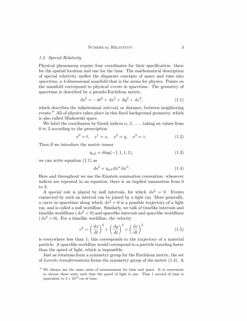
(a)
(b)
t0
t0 + ∆t
t0
t0 + ∆t
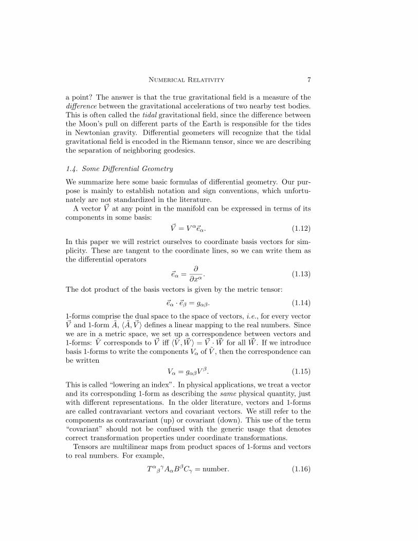
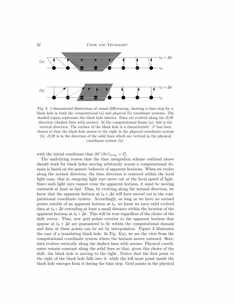
Fig. 3. 1-dimensional illustration of causal differencing, showing a time step for ablack hole in both the computational (a) and physical (b) coordinate systems. Theshaded region represents the black hole interior. Data are evolved along the ∂/∂tdirection (dashed lines with arrows). In the computational frame (a), this is thevertical direction. The surface of the black hole is a characteristic. βi has been
chosen so that the black hole moves to the right in the physical coordinate system(b). ∂/∂t is in the direction of the solid lines which are vertical in the physical
coordinate system (b).
with the initial conditions that ∂xi/∂xj |t=t0 = δij .The underlying reason that the time integration scheme outlined above
should work for black holes moving arbitrarily across a computational do-main is based on the generic behavior of apparent horizons. When we evolvealong the normal direction, the time direction is centered within the locallight cone, that is, outgoing light rays move out at the local speed of light.Since such light rays cannot cross the apparent horizon, it must be movingoutwards at least as fast. Thus, by evolving along the normal direction, weknow that the apparent horizon at t0 + ∆t will have moved out in the com-putational coordinate system. Accordingly, as long as we have no excisedpoints outside of an apparent horizon at t0, we know we have valid evolveddata at t0 +∆t extending at least a small distance within the location of theapparent horizon at t0 + ∆t. This will be true regardless of the choice of theshift vector. Thus, new grid points exterior to the apparent horizon thatappear at t0 + ∆t are guaranteed to lie within the computational domainand data at these points can be set by interpolation. Figure 3 illustratesthe case of a translating black hole. In Fig. 3(a), we see the view from thecomputational coordinate system where the horizon moves outward. Here,data evolves vertically along the dashed lines with arrows. Physical coordi-nates remain constant along the solid lines so that, given this choice of theshift, the black hole is moving to the right. Notice that the first point tothe right of the black hole falls into it, while the left-most point inside theblack hole emerges from it during the time step. Grid points in the physical
Numerical Relativity 33
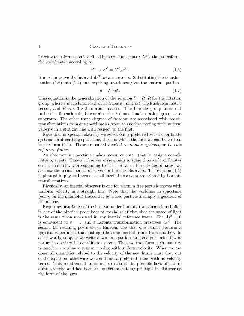
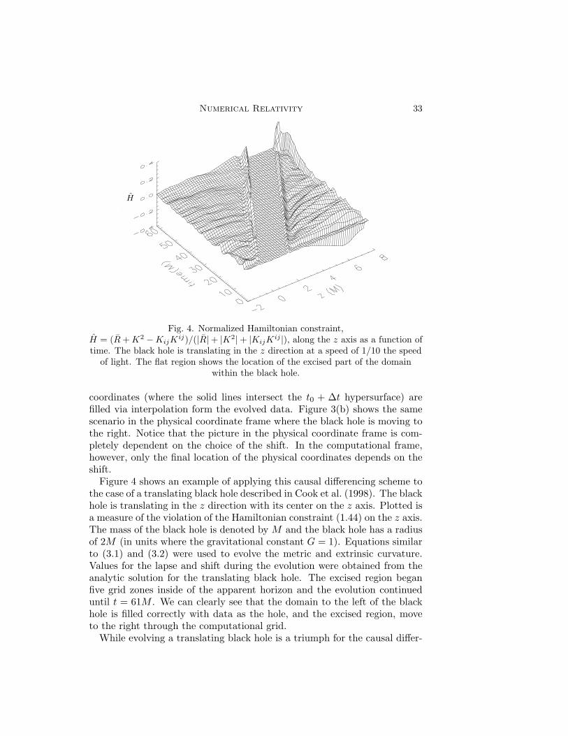
H
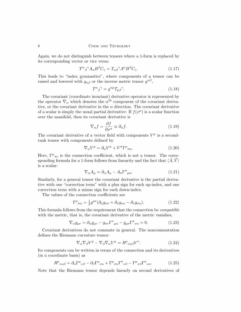
Fig. 4. Normalized Hamiltonian constraint,H = (R+K2 −KijK
ij)/(|R|+ |K2|+ |KijKij |), along the z axis as a function of
time. The black hole is translating in the z direction at a speed of 1/10 the speedof light. The flat region shows the location of the excised part of the domain
within the black hole.
coordinates (where the solid lines intersect the t0 + ∆t hypersurface) arefilled via interpolation form the evolved data. Figure 3(b) shows the samescenario in the physical coordinate frame where the black hole is moving tothe right. Notice that the picture in the physical coordinate frame is com-pletely dependent on the choice of the shift. In the computational frame,however, only the final location of the physical coordinates depends on theshift.
Figure 4 shows an example of applying this causal differencing scheme tothe case of a translating black hole described in Cook et al. (1998). The blackhole is translating in the z direction with its center on the z axis. Plotted isa measure of the violation of the Hamiltonian constraint (1.44) on the z axis.The mass of the black hole is denoted by M and the black hole has a radiusof 2M (in units where the gravitational constant G = 1). Equations similarto (3.1) and (3.2) were used to evolve the metric and extrinsic curvature.Values for the lapse and shift during the evolution were obtained from theanalytic solution for the translating black hole. The excised region beganfive grid zones inside of the apparent horizon and the evolution continueduntil t = 61M . We can clearly see that the domain to the left of the blackhole is filled correctly with data as the hole, and the excised region, moveto the right through the computational grid.
While evolving a translating black hole is a triumph for the causal differ-
34 Cook and Teukolsky
encing method, we are still a long way from generic 3-dimensional evolutions.The black hole in the above example is constructed from a spherically sym-metric solution using a simple coordinate transformation (a boost). Thisseverely limits the generality of the test, since spherically symmetric solu-tions to Einstein’s equations contain no true gravitational dynamics. Whilethe discrete nature of the numerics breaks the exact spherical symmetry,this is only at the level of a small perturbation. At present, there have beenno successful fully dynamical tests of apparent horizon boundary conditions.
To evolve truly dynamical black hole spacetimes one will need to considermore general shift vector choices than those considered so far. For example,to evolve a black hole binary system one may want to introduce the analog ofcorotating coordinates but without “twisting up” the coordinates around theindividual black holes, which will not in general rotate about their own axeswith the orbital angular velocity. A concern is that these general shift choicesmay introduce characteristic speeds into the system that exceed the speed oflight. This could be potentially disastrous when applying apparent horizonboundary conditions to the standard ADM evolution schemes, since “gaugewaves” could propagate out through the apparent horizon. One reason thathyperbolic formulations of general relativity are currently receiving so muchattention is that it is easy to compute the characteristic speeds and to besure that they are all physical.
3.4. Instabilities and Other Problems
Perhaps the most serious problem that has plagued the development ofschemes for evolving Einstein’s equations is the pervasiveness of instabil-ities. As we have mentioned before, there are currently no known generalevolution schemes that can evolve Einstein’s equations in three dimensionsfor an indefinite period of time. The possible sources of instability in anygeneral relativistic evolution scheme are many and varied.
First, the usual sorts of numerical instabilities such as the Courant-Friedrichs-Lewy instability for explicit evolution schemes can be handled trivially witha Courant condition. We might be concerned about the possible formationof shocks, given the nonlinear nature of Einstein’s equations. However, un-like Euler’s equations of fluid dynamics, the gravitational field equationsdo not develop shocks from smooth initial data (Choquet-Bruhat and York1980, Christodoulou and O Murchadha 1981). It is unknown whether thisanalytic result guarantees that shocks cannot form in a numerical solution.Moreover, if there are matter sources with shocks on the right-hand sidesof the gravitational equations, there will certainly be numerical difficulties.Hyperbolic formulations like the Einstein-Bianchi system have derivativesof the matter density, pressure, etc. as source terms, presumably makingthings worse. These problems have not been investigated yet. The situation
Numerical Relativity 35
is further complicated because a poor choice of the lapse or shift vector canintroduce steep gradients in the solution that look like shocks but are reallyjust coordinate singularities.
This problem with the choice of the shift is one aspect of a general classof problems that can occur in numerical evolutions of Einstein’s equations.As mentioned in §3.3, a particular choice of time slicing condition can leadto “grid stretching” in the vicinity of a black hole. This is again a coordi-nate (gauge) effect that ultimately leads to exponentially growing featuresin the solution. These coordinate effects are not really instabilities in thetraditional sense because they represent valid solutions of the equations.However, a poor choice of the gauge functions, the lapse and the shift, canlead to solutions with exponentially growing features that are difficult, butnot impossible, to distinguish from real instabilities. The way to diagnosethe presence of these “gauge instabilities” is to examine the growth of phys-ical, gauge independent quantities, or of violations of the constraints, whichare also gauge independent. Such quantities will not exhibit unstable growthif the instability is simply due to gauge effects. The problem with this ideais that without sufficient resolution, inaccuracies caused by growing gaugemodes will contaminate these indicators, making it difficult in practice todiagnose why a calculation is blowing up.
Also complicating the problem is the fact that the gauge freedom of gen-eral relativity yields a constrained evolution system. If the constraints arenot explicitly enforced during an evolution, then numerical errors will neces-sarily drive solutions away from the constraint surface. Not all formulationsof Einstein’s equations are stable when the constraints are violated. It isknown that the gauge-independent constraints do form a stable, symmetrichyperbolic system when γij and Kij are evolved via (3.1) and (3.2) (Frittelli1997). Unfortunately, the mathematically rigorous definition of stable evolu-tion used in this and other proofs may not be sufficient for numerical needs,since it guarantees only that perturbations do not grow faster than exponen-tially. Rapid power-law growth is often seen and quickly spoils numericalevolutions. This sort of constraint-violating instability can be diagnosed bythe unstable growth of gauge independent quantities. An example where aconstraint-violating instability was diagnosed and corrected in a simple 1-dimensional system can be found in Scheel et al. (1998). An interesting areaof investigation is whether a system of evolution equations can be writtenthat is attracted to the constraint surface (Brodbeck et al. 1998).
Certain choices of boundary conditions can also turn a stable evolutionscheme unstable. Of particular concern in this regard is the effect of ap-parent horizon boundary conditions on the overall stability of an evolutionscheme. Currently, there appears to be no good way to analyze the stabilityof various apparent horizon boundary conditions. Furthermore, there seemto be very few good tools for analyzing and diagnosing instabilities in gen-
36 Cook and Teukolsky
eral. The whole area of instabilities in evolution schemes is the outstandingcomputational problem in the field, and is urgently in need of further work.
3.5. Outer Boundary Conditions
Another issue that must be addressed is how to accurately and stably poseoutgoing wave boundary conditions in general relativity. The dynamicalsimulations of greatest interest are those that generate strong gravitationalwaves that will propagate towards infinity. The nonlinearity of Einstein’sequations couples ingoing and outgoing modes, implying that simple out-going wave boundary conditions must be applied at large radii where thecoupling is weak. The quadrupole nature of the dominant modes is a fur-ther complication when the outer boundary is not an S2 constant coordinatesurface.
Consider the apparently easy problem of setting Sommerfeld radiationconditions at the faces of a Cartesian grid for a simple scalar wave Φ(r, t).Assume that the solution is a purely outgoing wave given by
Φ(t, r) =f(t− r)
r. (3.19)
We can construct a boundary condition from the usual Sommerfeld relation
∂Φ∂r
= −1r
Φ− ∂Φ∂t, (3.20)
and the relations between Cartesian and spherical coordinates
∂
∂x=∂r
∂x
∂
∂r+∂θ
∂x
∂
∂θ+∂φ
∂x
∂
∂φ. (3.21)
Using the fact that f has no angular dependence, we get(∂r
∂x
)−1 ∂Φ∂x
= −1r
Φ− ∂Φ∂t, (3.22)
which can be applied easily at a constant x boundary.This works well for the simple monopole form given in (3.19). It even
works well at large radii if f(t − r)/r is just the leading order term in anexpansion for Φ(t, r, θ, φ) where the higher-order terms have angular depen-dence. But, if the leading-order term in the expansion has angular depen-dence, as is the case for the dominantly quadrupole gravitational radiation,(3.22) will not work, and straightforward Cartesian generalizations haveproven to be unstable for general relativistic problems. An approach thatwe term “interpolated-Sommerfeld” has proven to be a dramatic improve-ment. The idea is to apply (3.20) directly at the boundaries of a Cartesiangrid by using interpolation to provide data at points that are on radial linesassociated with the boundary points. This allows the radial derivative to be
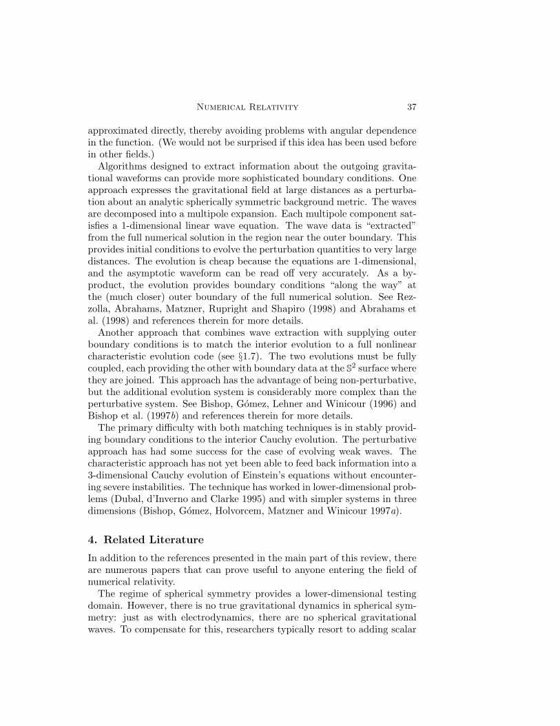
Numerical Relativity 37
approximated directly, thereby avoiding problems with angular dependencein the function. (We would not be surprised if this idea has been used beforein other fields.)
Algorithms designed to extract information about the outgoing gravita-tional waveforms can provide more sophisticated boundary conditions. Oneapproach expresses the gravitational field at large distances as a perturba-tion about an analytic spherically symmetric background metric. The wavesare decomposed into a multipole expansion. Each multipole component sat-isfies a 1-dimensional linear wave equation. The wave data is “extracted”from the full numerical solution in the region near the outer boundary. Thisprovides initial conditions to evolve the perturbation quantities to very largedistances. The evolution is cheap because the equations are 1-dimensional,and the asymptotic waveform can be read off very accurately. As a by-product, the evolution provides boundary conditions “along the way” atthe (much closer) outer boundary of the full numerical solution. See Rez-zolla, Abrahams, Matzner, Rupright and Shapiro (1998) and Abrahams etal. (1998) and references therein for more details.
Another approach that combines wave extraction with supplying outerboundary conditions is to match the interior evolution to a full nonlinearcharacteristic evolution code (see §1.7). The two evolutions must be fullycoupled, each providing the other with boundary data at the S2 surface wherethey are joined. This approach has the advantage of being non-perturbative,but the additional evolution system is considerably more complex than theperturbative system. See Bishop, Gomez, Lehner and Winicour (1996) andBishop et al. (1997b) and references therein for more details.
The primary difficulty with both matching techniques is in stably provid-ing boundary conditions to the interior Cauchy evolution. The perturbativeapproach has had some success for the case of evolving weak waves. Thecharacteristic approach has not yet been able to feed back information into a3-dimensional Cauchy evolution of Einstein’s equations without encounter-ing severe instabilities. The technique has worked in lower-dimensional prob-lems (Dubal, d’Inverno and Clarke 1995) and with simpler systems in threedimensions (Bishop, Gomez, Holvorcem, Matzner and Winicour 1997a).
4. Related Literature
In addition to the references presented in the main part of this review, thereare numerous papers that can prove useful to anyone entering the field ofnumerical relativity.
The regime of spherical symmetry provides a lower-dimensional testingdomain. However, there is no true gravitational dynamics in spherical sym-metry: just as with electrodynamics, there are no spherical gravitationalwaves. To compensate for this, researchers typically resort to adding scalar
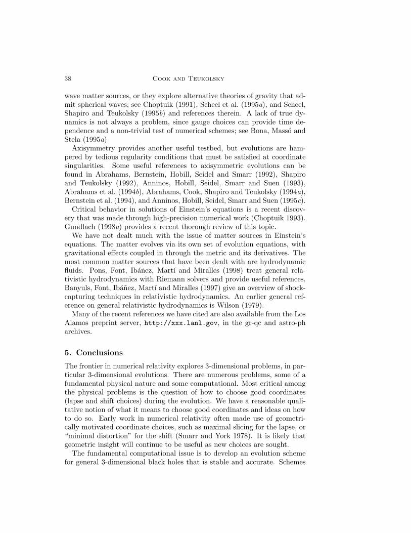
38 Cook and Teukolsky
wave matter sources, or they explore alternative theories of gravity that ad-mit spherical waves; see Choptuik (1991), Scheel et al. (1995a), and Scheel,Shapiro and Teukolsky (1995b) and references therein. A lack of true dy-namics is not always a problem, since gauge choices can provide time de-pendence and a non-trivial test of numerical schemes; see Bona, Masso andStela (1995a)
Axisymmetry provides another useful testbed, but evolutions are ham-pered by tedious regularity conditions that must be satisfied at coordinatesingularities. Some useful references to axisymmetric evolutions can befound in Abrahams, Bernstein, Hobill, Seidel and Smarr (1992), Shapiroand Teukolsky (1992), Anninos, Hobill, Seidel, Smarr and Suen (1993),Abrahams et al. (1994b), Abrahams, Cook, Shapiro and Teukolsky (1994a),Bernstein et al. (1994), and Anninos, Hobill, Seidel, Smarr and Suen (1995c).
Critical behavior in solutions of Einstein’s equations is a recent discov-ery that was made through high-precision numerical work (Choptuik 1993).Gundlach (1998a) provides a recent thorough review of this topic.
We have not dealt much with the issue of matter sources in Einstein’sequations. The matter evolves via its own set of evolution equations, withgravitational effects coupled in through the metric and its derivatives. Themost common matter sources that have been dealt with are hydrodynamicfluids. Pons, Font, Ibanez, Martı and Miralles (1998) treat general rela-tivistic hydrodynamics with Riemann solvers and provide useful references.Banyuls, Font, Ibanez, Martı and Miralles (1997) give an overview of shock-capturing techniques in relativistic hydrodynamics. An earlier general ref-erence on general relativistic hydrodynamics is Wilson (1979).
Many of the recent references we have cited are also available from the LosAlamos preprint server, http://xxx.lanl.gov, in the gr-qc and astro-pharchives.
5. Conclusions
The frontier in numerical relativity explores 3-dimensional problems, in par-ticular 3-dimensional evolutions. There are numerous problems, some of afundamental physical nature and some computational. Most critical amongthe physical problems is the question of how to choose good coordinates(lapse and shift choices) during the evolution. We have a reasonable quali-tative notion of what it means to choose good coordinates and ideas on howto do so. Early work in numerical relativity often made use of geometri-cally motivated coordinate choices, such as maximal slicing for the lapse, or“minimal distortion” for the shift (Smarr and York 1978). It is likely thatgeometric insight will continue to be useful as new choices are sought.
The fundamental computational issue is to develop an evolution schemefor general 3-dimensional black holes that is stable and accurate. Schemes
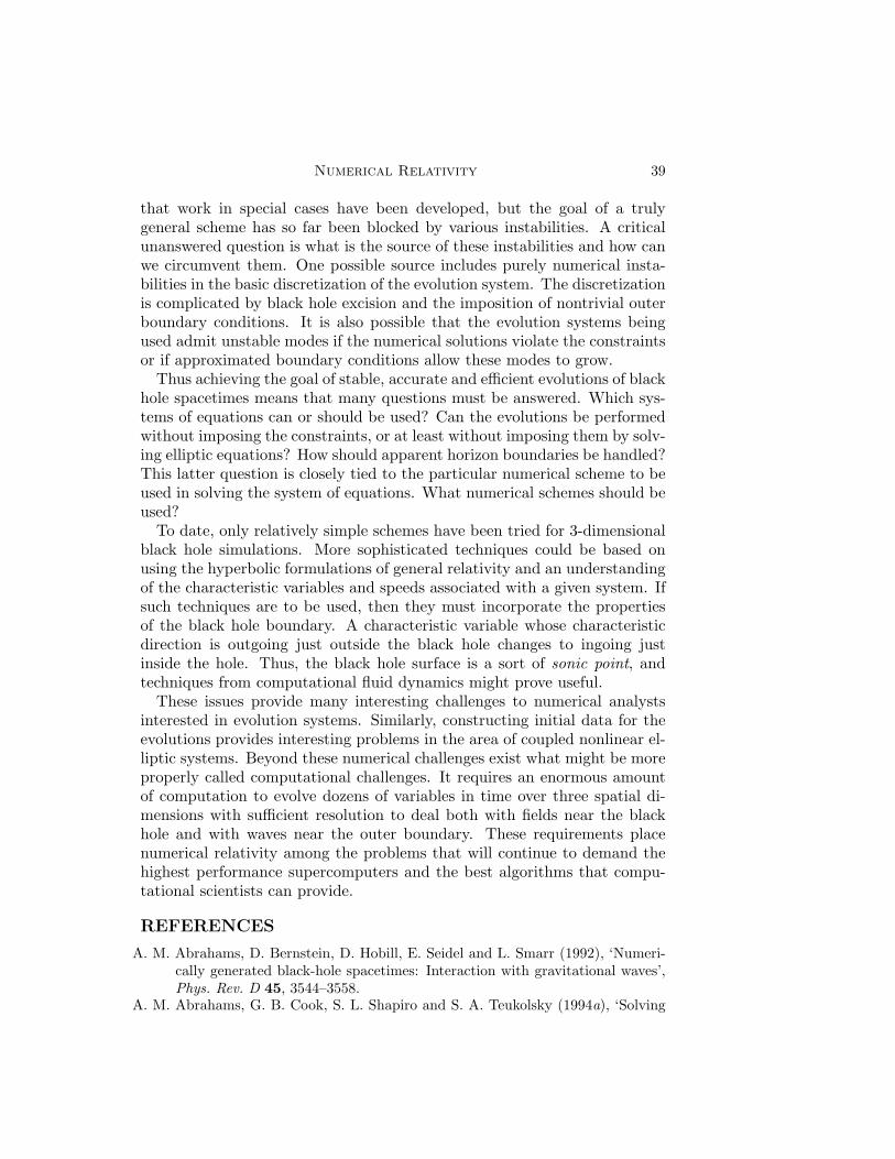
Numerical Relativity 39
that work in special cases have been developed, but the goal of a trulygeneral scheme has so far been blocked by various instabilities. A criticalunanswered question is what is the source of these instabilities and how canwe circumvent them. One possible source includes purely numerical insta-bilities in the basic discretization of the evolution system. The discretizationis complicated by black hole excision and the imposition of nontrivial outerboundary conditions. It is also possible that the evolution systems beingused admit unstable modes if the numerical solutions violate the constraintsor if approximated boundary conditions allow these modes to grow.
Thus achieving the goal of stable, accurate and efficient evolutions of blackhole spacetimes means that many questions must be answered. Which sys-tems of equations can or should be used? Can the evolutions be performedwithout imposing the constraints, or at least without imposing them by solv-ing elliptic equations? How should apparent horizon boundaries be handled?This latter question is closely tied to the particular numerical scheme to beused in solving the system of equations. What numerical schemes should beused?
To date, only relatively simple schemes have been tried for 3-dimensionalblack hole simulations. More sophisticated techniques could be based onusing the hyperbolic formulations of general relativity and an understandingof the characteristic variables and speeds associated with a given system. Ifsuch techniques are to be used, then they must incorporate the propertiesof the black hole boundary. A characteristic variable whose characteristicdirection is outgoing just outside the black hole changes to ingoing justinside the hole. Thus, the black hole surface is a sort of sonic point, andtechniques from computational fluid dynamics might prove useful.
These issues provide many interesting challenges to numerical analystsinterested in evolution systems. Similarly, constructing initial data for theevolutions provides interesting problems in the area of coupled nonlinear el-liptic systems. Beyond these numerical challenges exist what might be moreproperly called computational challenges. It requires an enormous amountof computation to evolve dozens of variables in time over three spatial di-mensions with sufficient resolution to deal both with fields near the blackhole and with waves near the outer boundary. These requirements placenumerical relativity among the problems that will continue to demand thehighest performance supercomputers and the best algorithms that compu-tational scientists can provide.
REFERENCES
A. M. Abrahams, D. Bernstein, D. Hobill, E. Seidel and L. Smarr (1992), ‘Numeri-cally generated black-hole spacetimes: Interaction with gravitational waves’,Phys. Rev. D 45, 3544–3558.
A. M. Abrahams, G. B. Cook, S. L. Shapiro and S. A. Teukolsky (1994a), ‘Solving
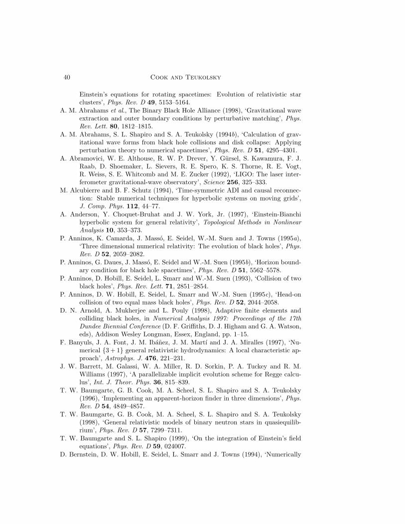
40 Cook and Teukolsky
Einstein’s equations for rotating spacetimes: Evolution of relativistic starclusters’, Phys. Rev. D 49, 5153–5164.
A. M. Abrahams et al., The Binary Black Hole Alliance (1998), ‘Gravitational waveextraction and outer boundary conditions by perturbative matching’, Phys.Rev. Lett. 80, 1812–1815.
A. M. Abrahams, S. L. Shapiro and S. A. Teukolsky (1994b), ‘Calculation of grav-itational wave forms from black hole collisions and disk collapse: Applyingperturbation theory to numerical spacetimes’, Phys. Rev. D 51, 4295–4301.
A. Abramovici, W. E. Althouse, R. W. P. Drever, Y. Gursel, S. Kawamura, F. J.Raab, D. Shoemaker, L. Sievers, R. E. Spero, K. S. Thorne, R. E. Vogt,R. Weiss, S. E. Whitcomb and M. E. Zucker (1992), ‘LIGO: The laser inter-ferometer gravitational-wave observatory’, Science 256, 325–333.
M. Alcubierre and B. F. Schutz (1994), ‘Time-symmetric ADI and causal reconnec-tion: Stable numerical techniques for hyperbolic systems on moving grids’,J. Comp. Phys. 112, 44–77.
A. Anderson, Y. Choquet-Bruhat and J. W. York, Jr. (1997), ‘Einstein-Bianchihyperbolic system for general relativity’, Topological Methods in NonlinearAnalysis 10, 353–373.
P. Anninos, K. Camarda, J. Masso, E. Seidel, W.-M. Suen and J. Towns (1995a),‘Three dimensional numerical relativity: The evolution of black holes’, Phys.Rev. D 52, 2059–2082.
P. Anninos, G. Daues, J. Masso, E. Seidel and W.-M. Suen (1995b), ‘Horizon bound-ary condition for black hole spacetimes’, Phys. Rev. D 51, 5562–5578.
P. Anninos, D. Hobill, E. Seidel, L. Smarr and W.-M. Suen (1993), ‘Collision of twoblack holes’, Phys. Rev. Lett. 71, 2851–2854.
P. Anninos, D. W. Hobill, E. Seidel, L. Smarr and W.-M. Suen (1995c), ‘Head-oncollision of two equal mass black holes’, Phys. Rev. D 52, 2044–2058.
D. N. Arnold, A. Mukherjee and L. Pouly (1998), Adaptive finite elements andcolliding black holes, in Numerical Analysis 1997: Proceedings of the 17thDundee Biennial Conference (D. F. Griffiths, D. J. Higham and G. A. Watson,eds), Addison Wesley Longman, Essex, England, pp. 1–15.
F. Banyuls, J. A. Font, J. M. Ibanez, J. M. Martı and J. A. Miralles (1997), ‘Nu-merical 3 + 1 general relativistic hydrodynamics: A local characteristic ap-proach’, Astrophys. J. 476, 221–231.
J. W. Barrett, M. Galassi, W. A. Miller, R. D. Sorkin, P. A. Tuckey and R. M.Williams (1997), ‘A parallelizable implicit evolution scheme for Regge calcu-lus’, Int. J. Theor. Phys. 36, 815–839.
T. W. Baumgarte, G. B. Cook, M. A. Scheel, S. L. Shapiro and S. A. Teukolsky(1996), ‘Implementing an apparent-horizon finder in three dimensions’, Phys.Rev. D 54, 4849–4857.
T. W. Baumgarte, G. B. Cook, M. A. Scheel, S. L. Shapiro and S. A. Teukolsky(1998), ‘General relativistic models of binary neutron stars in quasiequilib-rium’, Phys. Rev. D 57, 7299–7311.
T. W. Baumgarte and S. L. Shapiro (1999), ‘On the integration of Einstein’s fieldequations’, Phys. Rev. D 59, 024007.
D. Bernstein, D. W. Hobill, E. Seidel, L. Smarr and J. Towns (1994), ‘Numerically
Numerical Relativity 41
generated axisymmetric black hole spacetimes: Numerical methods and codetests’, Phys. Rev. D 50, 5000–5024.
N. T. Bishop, R. Gomez, P. R. Holvorcem, R. A. Matzner and P. P. J. Winicour(1997a), ‘Cauchy-characteristic evolution and waveforms’, J. Comp. Phys.136, 140–167.
N. T. Bishop, R. Gomez, L. Lehner and J. Winicour (1996), ‘Cauchy-characteristicextraction in numerical relativity’, Phys. Rev. D 54, 6153–6165.
N. T. Bishop, R. Gomez, L. Lehner, M. Maharaj and J. Winicour (1997b), ‘High-powered gravitational news’, Phys. Rev. D 56, 6298–6309.
C. Bona and J. Masso (1992), ‘A hyperbolic evolution system for numerical relativ-ity’, Phys. Rev. Lett. 68, 1097–1099.
C. Bona, J. Masso and J. Stela (1995a), ‘Numerical black holes: A moving gridapproach’, Phys. Rev. D 51, 1639–1639.
C. Bona, J. Masso, E. Seidel and J. Stela (1995b), ‘New formalism for numericalrelativity’, Phys. Rev. Lett. 75, 600–603.
S. Bonazzola, E. Gourgoulhon and J.-A. Marck (1997), ‘A relativistic formalism tocompute quasi-equilibrium configurations of non-synchronized neutron starbinaries’, Phys. Rev. D 56, 7740–7749.
S. Bonazzola, E. Gourgoulhon and J.-A. Marck (1998), ‘Numerical approach for highprecision 3-d relativistic star models’, Phys. Rev. D 58, 104020.
S. Bonazzola, E. Gourgoulhon and J.-A. Marck (1999), ‘Numerical models of irrota-tional binary neutron stars in general relativity’, Phys. Rev. Lett. submitted,LANL preprint archive, (astro-ph/9810072).
S. Bonazzola, E. Gourgoulhon, M. Salgado and J.-A. Marck (1993), ‘Axisymmetricrotating relativistic bodies: A new numerical approach for “exact” solutions’,Astron. Astrophys. 278, 421–443.
J. M. Bowen (1979), ‘General form for the longitudinal momentum of a sphericallysymmetric source’, Gen. Relativ. Gravit. 11, 227–231.
J. M. Bowen and J. W. York, Jr. (1980), ‘Time-asymmetric initial data for blackholes and black-hole collisions’, Phys. Rev. D 21, 2047–2056.
S. Brandt and B. Brugmann (1997), ‘A simple construction of initial data for multipleblack holes’, Phys. Rev. Lett. 78, 3606–3609.
S. R. Brandt and E. Seidel (1995), ‘The evolution of distorted rotating black holesI: Methods and tests’, Phys. Rev. D 52, 856–869.
O. Brodbeck, S. Frittelli, P. Hubner and O. A. Ruela (1998), ‘Einstein’s equationswith asymptotically stable constraint propagation’, J. Math. Phys. submitted,LANL preprint archive, (gr-qc/9809023).
B. Brugmann (1996), ‘Adaptive mesh and geodesically sliced Schwarzschild space-time in 3+1 dimensions’, Phys. Rev. D 54, 7361–7372.
E. M. Butterworth and J. R. Ipser (1976), ‘On the structure and stability of rapidlyrotating fluid bodies in general relativity. I. The numerical method for comput-ing structure and its application to uniformly rotating homogeneous bodies’,Astrophys. J. 204, 200–233.
M. W. Choptuik (1991), ‘Consistency of finite-difference solutions of Einstein’s equa-tions’, Phys. Rev. D 44, 3124–3135.
M. W. Choptuik (1993), ‘Universality and scaling in gravitational collapse of a mass-less scalar field’, Phys. Rev. Lett. 70, 9–12.
42 Cook and Teukolsky
Y. Choquet-Bruhat and J. W. York, Jr. (1980), The Cauchy problem, in Generalrelativity and gravitation. One hundred years after the birth of Albert Einstein(A. Held, ed.), Vol. 1, Plenum, New York, pp. 99–172.
Y. Choquet-Bruhat and J. W. York, Jr. (1995), ‘Geometrical well posed systems forthe Einstein equations’, C. R. Acad. Sci. Paris A321, 1089–1095.
D. Christodoulou and N. O Murchadha (1981), ‘The boost problem in general rela-tivity’, Commun. Math. Phys. 80, 271–300.
G. B. Cook (1991), ‘Initial data for axisymmetric black-hole collisions’, Phys. Rev.D 44, 2983–3000.
G. B. Cook (1994), ‘Three-dimensional initial data for the collision of two black holesII: Quasicircular orbits for equal mass black holes’, Phys. Rev. D 50, 5025–5032.
G. B. Cook and J. W. York, Jr. (1990), ‘Apparent horizons for boosted or spinningblack holes’, Phys. Rev. D 41, 1077–1085.
G. B. Cook, M. W. Choptuik, M. R. Dubal, S. Klasky, R. A. Matzner and S. R.Oliveira (1993), ‘Three-dimensional initial data for the collision of two blackholes’, Phys. Rev. D 47, 1471–1490.
G. B. Cook et al., The Binary Black Hole Alliance (1998), ‘Boosted three-dimensionalblack-hole evolutions with singularity excision’, Phys. Rev. Lett. 80, 2512–2516.
G. B. Cook, S. L. Shapiro and S. A. Teukolsky (1994), ‘Rapidly rotating neutron starsin general relativity: Realistic equations of state’, Astrophys. J. 424, 823–845.
M. R. Dubal, R. A. d’Inverno and C. J. S. Clarke (1995), ‘Combining Cauchy andcharacteristic codes II: The interface problem for vacuum cylindrical symme-try’, Phys. Rev. D 52, 6868–6881.
A. Einstein and N. Rosen (1935), ‘The particle problem in the general theory ofrelativity’, Phys. Rev. 48, 73–77.
C. R. Evans (1984), A Method for Numerical Relativity: Simulation of AxisymmetricGravitational Collapse and Gravitational Radiation Generation, PhD thesis,University of Texas at Austin.
A. E. Fischer and J. E. Marsden (1972), ‘The Einstein evolution equations as a first-order quasi-linear symmetric hyperbolic system, I’, Commun. Math. Phys.28, 1–38.
Y. Foures-Bruhat (1952), ‘Theorem d’existence pour certain systems d‘equations auxderivees partielles non lineaires’, Acta. Math. 88, 141–225.
J. L. Friedman, J. R. Ipser and L. Parker (1986), ‘Rapidly rotating neutron starmodels’, Astrophys. J. 304, 115–139.
H. Friedrich (1985), ‘On the hyperbolicity of Einstein’s and other gauge field equa-tions’, Commun. Math. Phys. 100, 525–543.
H. Friedrich (1996), ‘Hyperbolic reductions for Einstein’s equations’, Class. QuantumGravit. 13, 1451–1469.
S. Frittelli (1997), ‘Note on the propagation of the constraints in standard 3 + 1general relativity’, Phys. Rev. D 55, 5992–5996.
S. Frittelli and O. A. Reula (1996), ‘First-order symmetric hyperbolic Einstein equa-tions with arbitrary fixed gauge’, Phys. Rev. Lett. 76, 4667–4670.
A. P. Gentle and W. A. Miller (1998), ‘A fully (3+1)-d Regge calculus model of theKasner cosmology’, Class. Quantum Gravit. 15, 389–405.
Numerical Relativity 43
C. Gundlach (1998a), ‘Critical phenomena in gravitational collapse’, Adv. Theor.Math. Phys. 2, 1–49.
C. Gundlach (1998b), ‘Pseudo-spectral apparent horizon finders: An efficient newalgorithm’, Phys. Rev. D 57, 863–875.
S. W. Hawking and G. F. R. Ellis (1973), The Large Scale Structure of Spacetime,Cambridge University Press, Cambridge, England.
H. Komatsu, Y. Eriguchi and I. Hachisu (1989), ‘Rapidly rotating general relativisticstars – I. Numerical method and its application to uniformly rotating poly-tropes’, Mon. Not. R. astr. Soc. 237, 355–379.
A. D. Kulkarni (1984), ‘Time-asymmetric initial data for the N black hole problemin general relativity’, J. Math. Phys. 25, 1028–1034.
A. D. Kulkarni, L. C. Shepley and J. W. York, Jr. (1983), ‘Initial data for N blackholes’, Phys. Lett. 96A, 228–230.
R. L. Marsa and M. W. Choptuik (1996), ‘Black-hole-scalar-field interactions inspherical symmetry’, Phys. Rev. D 54, 4929–4943.
R. A. Matzner, M. F. Huq and D. Shoemaker (1998), ‘Initial data and coordinates formultiple black hole systems’, Phys. Rev. D. in press. LANL preprint archive,(gr-qc/9805023).
C. W. Misner (1963), ‘The method of images in geometrostatics’, Ann. Phys. 24, 102–117.
C. W. Misner, K. S. Thorne and J. A. Wheeler (1973), Gravitation, W. H. Freemanand Company, New York, New York.
N. O Murchadha and J. W. York, Jr. (1974), ‘Initial-value problem of general relativ-ity. I. General formulation and physical interpretation’, Phys. Rev. D 10, 428–436.
M. Parashar and J. C. Brown (1995), Distributed dynamical data-structures forparallel adaptive mesh-refinement, in Proceedings of the International Con-ference for High Performance Computing (S. Sahni, V. K. Prasanna andV. P. Bhatkar, eds), Tata McGraw-Hill, New Delhi, India. See alsowww.ticam.utexas.edu/∼parashar/public html/DAGH.
J. A. Pons, J. A. Font, J. M. Ibanez, J. M. Martı and J. A. Miralles (1998), ‘Generalrelativistic hydrodynamics with special relativistic Riemann solvers’, Astro.and Astroph. 339, 638–642.
T. Regge (1961), ‘General relativity without coordinates’, Nuovo Cimento 19, 558–571.
L. Rezzolla, A. M. Abrahams, R. A. Matzner, M. E. Rupright and S. L. Shapiro(1998), ‘Cauchy-perturbative matching and outer boundary conditions: Com-putational studies’, Phys. Rev. D. in press. LANL preprint archive, (gr-qc/9807047).
R. K. Sachs and H. Wu (1977), General Relativity for Mathematicians, Springer-Verlag, New York.
M. A. Scheel, T. W. Baumgarte, G. B. Cook, S. L. Shapiro and S. A. Teukolsky(1997), ‘Numerical evolution of black holes with a hyperbolic formulation ofgeneral relativity’, Phys. Rev. D 56, 6320–6335.
M. A. Scheel, T. W. Baumgarte, G. B. Cook, S. L. Shapiro and S. A. Teukolsky(1998), ‘Treating instabilities in a hyperbolic formulation of Einstein’s equa-tions’, Phys. Rev. D 58, 044020.

44 Cook and Teukolsky
M. A. Scheel, S. L. Shapiro and S. A. Teukolsky (1995a), ‘Collapse to black holesin Brans-Dicke theory. I. Horizon boundary conditions for dynamical space-times’, Phys. Rev. D 51, 4208–4235.
M. A. Scheel, S. L. Shapiro and S. A. Teukolsky (1995b), ‘Collapse to black holesin Brans-Dicke theory. II. Comparison with general relativity’, Phys. Rev. D51, 4236–4249.
E. Seidel and W.-M. Suen (1992), ‘Towards a singularity-proof scheme in numericalrelativity’, Phys. Rev. Lett. 69, 1845–1848.
S. L. Shapiro and S. A. Teukolsky (1992), ‘Collisions of relativistic clusters and theformation of black holes’, Phys. Rev. D 45, 2739–2750.
M. Shibata (1998), ‘A relativistic formalism for computation of irrotational binarystars in quasi-equilibrium states’, Phys. Rev. D 58, 024012/1–5.
L. L. Smarr and J. W. York, Jr. (1978), ‘Kinematical conditions in the constructionof spacetime’, Phys. Rev. D 17, 2529–2551.
R. D. Sorkin (1982), ‘A stability criterion for many-parameter equilibrium families’,Astrophys. J. 257, 847–854.
R. F. Stark and T. Piran (1987), ‘A general relativistic code for rotating axisymmetricconfigurations and gravitational radiation: Numerical methods and tests’,Computer Physics Reports 5, 221–264.
M. E. Taylor (1996), Partial Differential Equations III Nonlinear Equations,Springer-Verlag, New York.
S. A. Teukolsky (1998), ‘Irrotational binary neutron stars in quasiequilibrium ingeneral relativity’, Astrophys. J. 504, 442–449.
J. Thornburg (1987), ‘Coordinate and boundary conditions for the general relativisticinitial data problem’, Class. Quantum Gravit. 4, 1119–1131.
M. H. P. M. van Putten and D. M. Eardley (1996), ‘Hyperbolic reductions for Ein-stein’s equations’, Phys. Rev. D 53, 3056–3063.
R. M. Wald (1984), General Relativity, The University of Chicago Press, Chicago.R. M. Williams and P. A. Tuckey (1992), ‘Regge calculus: A brief review and bibli-
ography’, Class. Quantum Gravit. 9, 1409–1422.J. R. Wilson (1979), A numerical method for relativistic hydrodynamics, in Sources
of Gravitational Radiation (L. L. Smarr, ed.), Cambridge University Press,Cambridge, England, pp. 423–445.
J. R. Wilson, G. J. Mathews and P. Marronetti (1996), ‘Relativistic numericalmethod for close neutron star binaries’, Phys. Rev. D 54, 1317–1331.
J. W. York, Jr. (1979), Kinematics and dynamics of general relativity, in Sourcesof Gravitational Radiation (L. L. Smarr, ed.), Cambridge University Press,Cambridge, England, pp. 83–126.


