INSTITUTE OF PHYSICS PUBLISHING CLASSICAL AND QUANTUM GRAVITY

Class. Quantum Grav. 22 (2005) 425–451 doi:10.1088/0264-9381/22/2/014

Numerical relativity using a generalized harmonicdecomposition

Frans Pretorius

Theoretical Astrophysics, California Institute of Technology, Pasadena, CA 91125, USA

Received 30 July 2004, in final form 6 December 2004Published 3 January 2005Online at stacks.iop.org/CQG/22/425

AbstractA new numerical scheme to solve the Einstein field equations based upon thegeneralized harmonic decomposition of the Ricci tensor is introduced. Thesource functions driving the wave equations that define generalized harmoniccoordinates are treated as independent functions, and encode the coordinatefreedom of solutions. Techniques are discussed to impose particular gaugeconditions through a specification of the source functions. A 3D, free evolution,finite difference code implementing this system of equations with a scalarfield matter source is described. The second-order-in-space-and-time partialdifferential equations are discretized directly without the use of first-orderauxiliary terms, limiting the number of independent functions to 15—ten metricquantities, four source functions and the scalar field. This also limits the numberof constraint equations, which can only be enforced to within truncation errorin a numerical free evolution, to four. The coordinate system is compactified tospatial infinity in order to impose physically motivated, constraint-preservingouter boundary conditions. A variant of the cartoon method for efficientlysimulating axisymmetric spacetimes with a Cartesian code is described thatdoes not use interpolation, and is easier to incorporate into existing adaptivemesh refinement packages. Preliminary test simulations of vacuum black-hole evolution and black-hole formation via scalar field collapse are described,suggesting that this method may be useful for studying many spacetimes ofinterest.

PACS numbers: 04.25.Dm, 04.40.−b, 04.70.Bw

1. Introduction

One of the primary goals of numerical relativity today is to solve for astrophysical spacetimesthat are expected to be strong sources of gravitational wave emission in the frequency bandsrelevant to current and planned gravitational wave detectors. Expected sources include the

0264-9381/05/020425+27$30.00 © 2005 IOP Publishing Ltd Printed in the UK 425

426 F Pretorius

inspiral and merger of compact objects, supernovae, pulsars and the big bang. An importanttool for extracting physics from detector signals is the technique of matched filtering, whichrequires an accurate waveform of a model of the expected source. For binary black-holemergers (in particular) it is thought that numerical relativity is the only method that will beable to provide such waveforms close to and during the plunge phase of the merger. Despitesignificant progress made over the past decade, a full solution to this problem still eludesresearches. One reason for the difficulty is the complexity of the field equations. Thistranslates into significant computer resources being needed to solve the equations, whichlimits the turn-around time for testing new ideas. However, perhaps the largest obstacle sofar has been finding a formalism to write the field equations in that is amenable to long-term, stable numerical evolution. Some of the promising techniques used today includesymmetric hyperbolic formalisms [1, 2], the BSSN formalism (sometimes referred to as theNOK formalism) [3–6] and characteristic evolution (for black-hole/neutron-star systems) [7].Several groups are also beginning to examine the possibility of constrained evolution forthe 3D binary black-hole problem [8–10], and other promising directions make use oftetrad formulations of the field equations [12–14], and solution of the conformal fieldequations [15–18].

A method of writing the field equations that has proven very useful in analytic studiesis arrived at by imposing the harmonic coordinate condition, where the four spacetimecoordinates xµ are chosen to individually satisfy wave equations: �xµ = 0. The Einsteinequations, when written with this condition imposed, take on a mathematically appealing formwhere the principal part of each partial differential equation satisfied by a metric componentgαβ becomes the scalar wave operator �gαβ . This allowed for (among other things) thefirst existence and uniqueness proof of solutions to the field equations [19]. In numericalrelativity, a solution scheme based directly upon this formulation of the field equations hasrecently been suggested by Garfinkle [20] (see also related work by Szilagyi and Winicour[21], and the so-called Z4 system [22], which seems to be quite similar to generalized harmonicevolution in many respects). Garfinkle considered a generalization of the harmonic coordinatecondition of the form � xµ = Hµ, where Hµ are now arbitrary source functions, and foundthat the technique was successful in simulations of the approach to the singularity in certaincosmological spacetimes.

One purpose of this paper is to begin to investigate the use of the generalized harmonicdecomposition in asymptotically flat spacetimes. The formalism is described in section 2. Ifthis method is to be useful for a large class of spacetimes, one issue that needs to be addressedis how to choose gauge conditions via specification of the source functions Hµ; this topic isdiscussed in section 3. A second goal of this paper is to investigate direct discretization ofthe second-order-in-space-and-time partial differential equations1 (in other words, the systemis not converted into a system of first-order equations before discretization). One reason fordoing so is to have a free evolution scheme where the only constraints amongst the variables arethe four constraint equations imposed by the Einstein equations (see also [24, 21]). The hopethen is that even if this system suffers from ‘constraint violating modes’2, it may be easier toanalyse and cure them using (for instance) ideas suggested in research of symmetric hyperbolic

1 Recent analytic investigations by Calabrese [23] have suggested that such a scheme may suffer from high-frequencyinstabilities in situations where the coefficients in front of mixed time–space derivatives are greater than the localcharacteristic speed. We have not yet noticed such an instability, probably because of the numerical dissipation weuse, which was one of the suggested cures for the problem in [23].2 By constraint violating mode we mean a solution to the continuum evolution equations that is not a solution of thefull Einstein equations, and furthermore exhibits exponential growth from initial data with arbitrarily small deviationsfrom putative initial data that does satisfy the constraints.

Numerical relativity using a generalized harmonic decomposition 427

versions of the field equations [25–29]3. The numerical code is described in section 4,along with related topics such as apparent horizon finding, excision, boundary conditions,initial conditions and the current scalar field matter source. Also described in section 4 isa variant of the cartoon method [32] to efficiently simulate axisymmetric spacetimes with aCartesian code. The advantages of the method presented here are that no interpolation is used,and the axisymmetric simulation is performed on a two-dimensional slice of the Cartesiangrid. In section 5 test simulations of black-hole evolution and gravitational collapse areshown, suggesting that this solution method holds promise for simulating asymptotically flatspacetimes. Concluding remarks are given in section 6, in particular, a discussion of someof the work that still needs to be done before the code could provide new physical results insituations of interest.

2. The Einstein field equations in the generalized harmonic decomposition

Consider the Einstein field equations in the form

Rαβ = 4π(2Tαβ − gαβT ), (1)

where Rαβ is the Ricci tensor, gαβ is the metric tensor, Tαβ is the stress–energy tensor withtrace T, and units have been chosen so that Newton’s constant G and the speed of light c areequal to 1. The Ricci tensor is defined in terms of the Christoffel symbols �

γ

αβ by

Rαβ = �δαβ,δ − �δ

δβ,α + �εαβ�δ

εδ − �εδβ�δ

εα (2)

where �γ

αβ is

�γ

αβ = 12gγ ε[gαε,β + gβε,α − gαβ,ε]. (3)

The notation f,α and ∂αf is used interchangeably to denote ordinary differentiation of somequantity f with respect to the coordinate xα .

Introduce a set of four source functions Hµ via

Hµ ≡ �xµ (4)

= 1√−g∂α

(√−ggαβxµ,β

)(5)

= 1√−g∂α(

√−ggαµ), (6)

or, equivalently, defining Hµ = gµνHν , we have

Hµ = (ln√−g),µ − gανgνµ,α. (7)

The symmetrized gradient of Hµ is thus

H(µ,ν) = (ln√−g),µν − gαβ

(,νgµ)β,α − gαβgβ(µ,ν)α. (8)

The generalized harmonic decomposition involves replacing particular combinations of firstand second derivatives of the metric in the Ricci tensor (2) by the equivalent quantities in(7), (8), and then promoting the source functions Hµ to the status of independent quantities.Specifically, one can rewrite the field equations (1) as

gδγ gαβ,γ δ + gγ δ,βgαδ,γ + gγ δ

,αgβδ,γ + 2H(α,β) − 2Hδ�δαβ + 2�

γ

δβ�δγα = −8π(2Tαβ − gαβT ).

(9)

3 For it appears that it may not be possible to construct a constrained–transport-type numerical evolution scheme thatsatisfies all of the Einstein equations to machine precision [30, 31].

428 F Pretorius

As Hµ are now four independent functions, one needs to provide four additional, independentdifferential equations to solve for them, which we write schematically as

LµHµ = 0 (no summation). (10)

Lµ is a differential operator that in general can depend upon the spacetime coordinates, themetric and its derivatives, and the source functions and their derivatives. Note however thatthe principal part of (9) is now the simple wave operator gδγ ∂γ ∂δ acting upon each metriccomponent gαβ ; this subsystem of equations is manifestly hyperbolic given certain reasonableconditions on the metric4 and as long as the coupling between (9), (10) and any matter evolutionequations that may be needed do not the affect the characteristic structure of (9). We will notdiscuss the well-posedness of this system of equations here, though this is certainly a topicworth pursuing.

The Einstein field equations are thus equivalent to the system of equations (9) and (10),provided that the harmonic ‘constraints’ (7) are satisfied for all time t ≡ x0. The claim thenis that, at the analytical level, if (9) is used to that evolve gαβ , and (10) is used to evolve Hµ,then (7) will be satisfied for all time provided that initial conditions are specified so that (7)and (8) are satisfied then. For the special case where Hµ are given as a priori functions of thecoordinates xµ, the preceding statement has been proven before [33] (the case Hµ = 0 wasfirst shown in [19]). The idea behind the proof is as follows. Define the harmonic constraintfunction Cµ as

Cµ ≡ Hµ − � xµ. (11)

For any solution to the Einstein equations (1), Cµ is identically zero. Using the contractedBianchi identity and conservation of stress energy, one can show that Cµ satisfies the followinghomogeneous wave equation:

�Cµ = −RµνC

ν. (12)

Therefore, given any gµν that satisfies (9) for all time together with some Hµ that satisfiesboth Cµ = 0 and ∂tC

µ = 0 at t = 0, (12) guarantees that gµν will also solve the Einsteinequations (1) for all time. We cannot prove such a result for a general evolution system whereHµ is specified via some arbitrary set of differential equations. Rather, we will take themore pragmatic approach in the numerical code of demonstrating convergence to a solution ofthe Einstein equations for any particular evolution system we use. In fact, such a convergencetest is the only measure of the validity of the numerical solution, regardless of any analyticproperties of the underlying continuum problem.

Equivalent to enforcing (8) at t = 0 is to make sure that the usual constraint equations,namely

(3)R + K2 − KabKab = 16πρ, (13)

K ba |b − K|a = 8πJa (14)

are satisfied then, which from a practical standpoint is easier to solve than (8) using existing,well-established techniques [2, 42]. In the above, Kab is the extrinsic curvature tensor of thet = const hypersurface with the induced metric hab,K is the trace of Kab, (3)R is the Ricciscalar of hab, | denotes the covariant derivative operator compatible with hab, and ρ and Ja arethe projected matter energy and momentum densities respectively. Note that we use notationwhere Greek indices denote four-dimensional quantities and run from 0 to 3, and Latin indicesdenote three-dimensional spatial quantities and run from 1 to 3.

4 For example one would need a single coordinate to be timelike and the rest to be spacelike throughout the integrationvolume.

Numerical relativity using a generalized harmonic decomposition 429

At this stage the system (9), (10) is completely general in that we have not yet specifiedany time slicing or spatial coordinates. Choosing a gauge amounts to specifying a set ofsource functions through (10), and thus the source functions play a role analogous to the lapsefunction and shift vector in the traditional ADM decomposition. One disadvantage of theharmonic decomposition is that (to my knowledge) there is no simple geometric descriptionof the relationship between Hµ and the resulting spacetime coordinates. In same cases onecan appeal to the ADM lapse and shift view of coordinate freedom to motivate a particularchoice of Hµ. We will discuss these and several other classes of gauge conditions that may beuseful for numerical evolution in the following section.

3. Specifying a gauge

Within the generalized harmonic decomposition one can think of the source functions Hµ asrepresenting the four coordinate degrees of freedom available in general relativity. There aremany conceivable ways of choosing Hµ; in this section we will give a few suggestions, severalof which are used in the evolutions presented in section 5. However, the discussion here israther heuristic in that we do not consider how any of these gauge choices may affect thecharacter of the coupled Einstein-gauge evolution system. Note that gauge source functionswere discussed by Friedrich [43] in some detail, though not specifically within the context ofsupplying additional evolution equations for them.

The simplest gauge choice in this formalism is to set the source functions equal to somearbitrary functions of the spacetime coordinates:

Hµ = fµ(xα). (15)

The case fµ = 0 is standard harmonic coordinates. The next condition we consider is acoordinate system that evolves towards harmonic coordinates:

∂tHµ = −κµ(t)Hµ (no summation), (16)

where κµ are a set of four arbitrary though positive functions of time, which if non-zero willcause Hµ to evolve to zero.

A useful method to derive coordinate conditions for the harmonic decomposition is toappeal to the manner in which the coordinate system is specified in the ADM decomposition.This makes available a tremendous amount of research that has gone into gauge related issuesfor the ADM-based evolution [2]. In the ADM formalism the metric element is written as

ds2 = −α2 + hij (dxi + βi dt)(dxj + βj dt), (17)

where the lapse function α measures the rate of change of proper time with respect to coordinatetime t of hypersurface normal observers, hij is the intrinsic metric of t = const slices, and theshift vector βj describes how the spatial coordinates change for normal observers from onetime slice to the next. The normal component and spatial projection of the source function Hµ

are5

H · n ≡ Hµnµ

= −K − ∂ν(ln α)nν (18)⊥Hi ≡ Hµhµi

= −�ijkh

jk + ∂j (ln α)hij +1

α∂γ βinγ , (19)

5 Note however that Hµ does not transform as a one-form under coordinate transformations, and hence the projectionsare not covariant objects.

430 F Pretorius

where �ijk is the connection associated with hij , and nν is the hypersurface normal vector

given by

nν = −α∂νt. (20)

Note that in (18) and (19) the time derivative of α only appears in H · n, while the timederivative of βi only appears in the corresponding component of ⊥Hi . In other words, thechoice of the normal component H · n in an evolution directly affects the rate of change of α

with respect to time, and therefore H · n controls the time-slicing of the spacetime; similarly,⊥Hi controls the manner in which the spatial coordinates evolve with time (another way ofstating this is that (18), (19) are generalizations of the hyperbolic equations governing thelapse and shift within harmonic coordinates [44]). One way in which an ADM style gaugecondition can be used within the harmonic decomposition is to substitute the correspondingchoices of α and βi into (18), (19), and use the result as the source functions for the harmonicevolution. The simplest class of gauge conditions that can be implemented in this fashion arethe so-called ‘driver’ conditions [45–49], where one directly specifies the time derivatives ofα and βi to achieve, for example, approximate maximal slicing and minimal distortion gaugesrespectively.

The manner in which the ADM driver conditions are implemented suggests a similar wayin which such gauge conditions can be used in a harmonic evolution: instead of substitutingin the forms for α and βi in (18), (19) to try to satisfy the conditions exactly, choose sourcefunctions to drive the gauge towards the desired one. To see how this can be done, first rewrite(18), (19) as evolution equations for the lapse and shift:

∂tα = −α2H · n + · · · (21)

∂tβi = α2 ⊥ Hi + · · · , (22)

where the ellipses denote the rest of the terms that do not contain ∂tα, ∂tβi or Hµ. Now

suppose at some instant of time the desired value of the lapse and shift are calculated (bywhatever means) to be α0 and βi

0 respectively. Then from (21), (22) one possible set of choicesfor the source functions that will cause the lapse and shift to evolve towards the desired valuesare

H · n = κn(t)α − α0

α2(23)

⊥Hi = −κi(t)βi − βi

0

α2(no summation), (24)

where κn and κi are positive functions of time that can be used to control the rate of evolution.It many circumstances it may make more sense to implement the above style driver

conditions as evolution equations, rather than algebraic conditions. This could be, for example,if the initial conditions for Hµ are not compatible with the desired gauge choice, and soimplementing (23), (24) will result in discontinuous source functions at the initial time. Acouple of alternative possibilities include

∂H · n

∂t= κn(t)

α − α0

α2(25)

and

�(H · n) = −κn(t)α − α0

α2+ ξn(t)(H · n),µnµ, (26)

with similar expressions for the spatial parts of Hµ. ξn(t) is a positive function that can beused to add a dissipative term to (26). One advantage of using a wave operator (26) to evolve

Numerical relativity using a generalized harmonic decomposition 431

the source functions is then the principal parts of all equations in the system (9), (10) havethe same characteristic structure (as long as α0 and βi

0 depend at most on first derivativesof the fundamental variables). This may be important to establish well-posedness of thecoupled system of equations [50].

It is beyond the scope of this paper to investigate how well any of these suggestedgauge conditions performs in situations of interest; however in section 5 we will show somepreliminary results indicating that these ideas can be implemented in a stable fashion.

4. Numerical code

In this section we describe a 3D numerical code based upon the generalized harmonicdecomposition. This code has several features of note.

• Direct discretization of (9), (10). In other words, we do not convert the system of equationsinto the first-order form—the only variables used are the ten unique metric componentsgαβ , four source functions Hµ and matter variables.

• Spatially compactified Cartesian coordinates. The spatial coordinates are compactifiedto include i0, to simplify the imposition of physically realistic boundary conditions forasymptotically flat spacetimes.

• Black-hole excision. Black-hole excision is used to evolve spacetimes containing blackholes, whereby portions of the computational domain inside apparent horizons are‘excised’ to remove the singularities.

• Built within a parallel adaptive mesh refinement (AMR) framework. The code utilizes anew set of parallel AMR libraries which we will describe elsewhere, though the Bergerand Oliger style AMR algorithm used is very similar to the one presented in [51, 52].

• Efficient simulation of axisymmetric spacetimes using a variant of the Cartoon method[32]. The algorithm presented here does not require interpolation, and only utilizes asingle two-dimensional slice of the Cartesian grid, simplifying incorporation into existingAMR packages.

In the remainder of this section we will describe certain aspects of the code in more detail.

4.1. Discretization scheme

Here onwards we will use the coordinate names t ≡ x0 and (x, y, z) ≡ (x1, x2, x3). Also,as discussed in the next section, we use a compactified coordinate system in the code. Thisnecessitates the use of regularized variables for some of the metric and source functioncomponents; however to keep the discussion in this section simpler we ignore that aspect ofthe code here. In appendix B we present a stability analysis of this discretization methodapplied to a one-dimensional wave equation in flat space. The purpose of the analysis isto give a simple, concrete example of the numerical method, and to show that there are nofundamental instabilities in it. Of course, this cannot prove that the full, nonlinear problem incompactified coordinates will be stable—doing so is beyond the scope of this paper.

We use second-order accurate finite difference techniques to discretized (9), (10) and thescalar field evolution equation (45) presented in section 4.4. This is a set of 15 equations for 15unknown functions—the ten non-trivial metric components gαβ , the four source functions Hµ

and the scalar field . In the discretized version of (9) all Christoffel symbols, contravariantmetric elements and their gradients are replaced with the appropriate sum of covariantmetric elements and their gradients. As (9) and (45) are second-order partial differentialequations in time, second-order accurate discretization requires a three time-level scheme

432 F Pretorius

fn+1i

fni fn

i+1fni−1

fn−1i

tn

tn+1

tn−1

xi xi+1xi−1

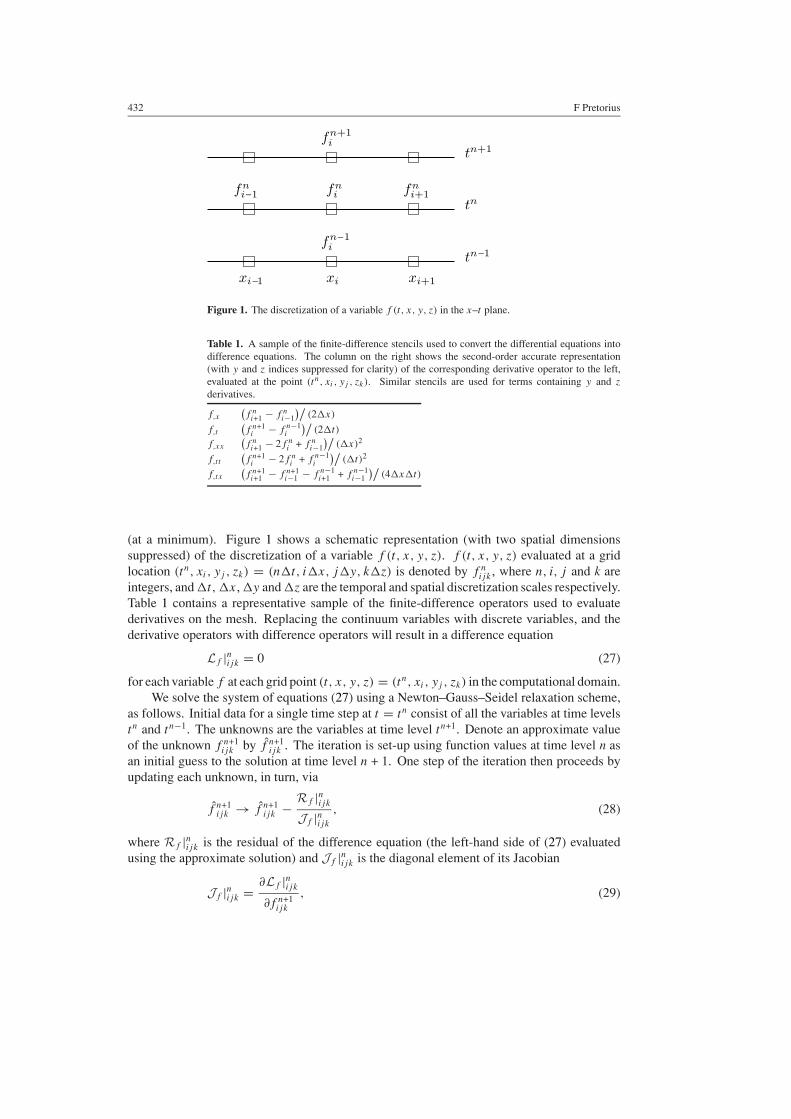
Figure 1. The discretization of a variable f (t, x, y, z) in the x–t plane.

Table 1. A sample of the finite-difference stencils used to convert the differential equations intodifference equations. The column on the right shows the second-order accurate representation(with y and z indices suppressed for clarity) of the corresponding derivative operator to the left,evaluated at the point (tn, xi , yj , zk). Similar stencils are used for terms containing y and z

derivatives.

f,x

(f n

i+1 − f ni−1

)/(2�x)

f,t

(f n+1

i − f n−1i

)/(2�t)

f,xx

(f n

i+1 − 2f ni + f n

i−1

)/(�x)2

f,tt

(f n+1

i − 2f ni + f n−1

i

)/(�t)2

f,tx

(f n+1

i+1 − f n+1i−1 − f n−1

i+1 + f n−1i−1

)/(4�x�t)

(at a minimum). Figure 1 shows a schematic representation (with two spatial dimensionssuppressed) of the discretization of a variable f (t, x, y, z). f (t, x, y, z) evaluated at a gridlocation (tn, xi, yj , zk) = (n�t, i�x, j�y, k�z) is denoted by f n

ijk , where n, i, j and k areintegers, and �t,�x, �y and �z are the temporal and spatial discretization scales respectively.Table 1 contains a representative sample of the finite-difference operators used to evaluatederivatives on the mesh. Replacing the continuum variables with discrete variables, and thederivative operators with difference operators will result in a difference equation

Lf |nijk = 0 (27)

for each variable f at each grid point (t, x, y, z) = (tn, xi, yj , zk) in the computational domain.We solve the system of equations (27) using a Newton–Gauss–Seidel relaxation scheme,

as follows. Initial data for a single time step at t = tn consist of all the variables at time levelstn and tn−1. The unknowns are the variables at time level tn+1. Denote an approximate valueof the unknown f n+1

ijk by f n+1ijk . The iteration is set-up using function values at time level n as

an initial guess to the solution at time level n + 1. One step of the iteration then proceeds byupdating each unknown, in turn, via

f n+1ijk → f n+1

ijk − Rf |nijk

Jf |nijk

, (28)

where Rf |nijk is the residual of the difference equation (the left-hand side of (27) evaluatedusing the approximate solution) and Jf |nijk is the diagonal element of its Jacobian

Jf |nijk = ∂Lf |nijk

∂f n+1ijk

, (29)

Numerical relativity using a generalized harmonic decomposition 433

again evaluated with the approximate solution. In other words, (28) is simply solving alinearized version of (27) for f n+1

ijk assuming all other unknowns are fixed. The iteration isrepeated until the residual for all variables is below some specified tolerance.

4.1.1. Numerical dissipation. Some form of numerical dissipation is necessary to stablyevolve certain spacetimes, in particular those that contain black holes. We use Kreiss–Oliger-style dissipation [53]; however, rather than modify the discrete evolution equations as istypically done (and note also that [53] considered first order in time systems), we apply thedissipation as a filter to the discrete variables, at both past time levels tn and tn−1, prior toupdating tn+1. Specifically, at a given time level we define the high-frequency component ηx

ijk

of grid function fijk , in the x direction, as

ηxijk = 1

16 (fi−2jk − 4fi−1jk + 6fijk − 4fi+1jk + fi+2jk), 2 < i < Nx − 2

= 0 elsewhere, (30)

where the local size of the mesh is Nx points in the x direction. After ηxijk has been calculated

over the entire local grid, it is subtracted from f as follows:

fijk = fijk − εηxijk, (31)

where ε is a constant, required to be in the range 0 . . . 1 for stability. In practice we use valuesof ε in the range 0.2 to 0.5. Once the high-frequency components in the x direction have beensubtracted, the procedure is repeated for the high-frequency components η

y

ijk and ηzijk of fijk

in the y and z directions respectively, which are given by expressions similar to (30).We did experiment with extending the dissipation filter to the grid boundaries as outlined

in [54]; however this did not seem to have a significant effect on the solution in mostcircumstances, and seemed to produce more error (as measured by residuals of the fieldequations) next to excision boundaries without offering improved stability. However, theexcision method proposed in [54] was for cubical excision boundaries, and for schemessatisfying summation by parts, so it is questionable how appropriate it is to apply that methodhere. Also note that applying the above filters to both past time levels at each evolution stepis essential for long-term stability. We do not know why this is so important; naively onewould think that only applying the filter to time level tn would be sufficient, as the update stepdoes not alter the variables at tn, and since tn is copied to tn−1 after each update step, bothtn and tn−1 are effectively smoothed. Also, a simple extension of the analysis in appendix Bto account for different amounts of dissipation applied to each of the past time levels showsthat the one-dimensional, flat space wave equation remains stable; hence the need to dissipateboth time levels is particular to black-hole spacetimes as far as we can tell.

4.2. Coordinate system and boundary conditions

To simplify the imposition of asymptotically flat boundary conditions we use the followingspatially compactified coordinate system. First, consider an uncompactified Cartesiancoordinate system of the form

ds2 = gtt dt2 + 2gti dxi dt + gij dxi dxj . (32)

Here (x1, x2, x3) ≡ (x, y, z) runs from −∞ to +∞, and in the limit where xi → ±∞ themetric becomes the Minkowski metric

ds2 = −dt2 + dx2 + dy2 + dz2. (33)

The following coordinate transformation

xi = tan(πxi/2) (34)

434 F Pretorius

(with t = t) will bring (32) into the form

ds2 = gtt dt2 + 2gti dxi dt + gij dxi dxj , (35)

where

gti = π

2sec2(πxi/2)gti ,

gij = π2

4sec2(πxi/2) sec2(πxj/2)gij .

(36)

Now xi runs from −1 to 1, and spacelike infinity i0 corresponds to the surfaces xi = ±1.Note that in this limit the compactified (unbarred) metric elements are singular; however theuncompactified parts are still well behaved and asymptote to their Minkowski values. In thecode we thus evolve the uncompactified components gtt , gti and gij , analytically substitutingthe values (36) into (9) prior to discretization. Furthermore, in the compactified coordinatesystem (35) we define the spatial source functions Hi to take the form

Hi = H i − π tan(πxi/2) (37)

and evolve only the regularized components H i (for note that in compactified Minkowskicoordinates Hi = π tan(πxi/2) from (7)). Therefore, the outer boundary conditions weimpose on the regularized metric and source functions are

gtt (t, i0) = −1, gti (t, i

0) = 0,

gii (t, i0) = 1, gij (t, i

0) = 0, i �= j

Ht(t, i0) = 0, H i(t, i

0) = 0,

(38)

where the notation (t, i0) refers to any one of the six boundaries x = ±1, y = ±1 and z = ±1.We conclude this section by discussing several concerns about evolving the field equations

in a coordinate system compactified to spatial infinity. It is beyond the scope of this paper toanalyse these issues in more detail; however, we are currently investigating them. However,note that a similar compactification scheme was used to model black strings in five dimensions[38], with no notable adverse effects.

First, the metric, hence equations, are formally singular at i0. The singular behaviour isdealt with using regularized variables and enforcing Minkowski space boundary conditions ati0, as described above. Nevertheless, there are terms in the equations that grow as 1/h4 atgrid locations near the outer boundary, where h is the mesh spacing there. Therefore, for theequations to remain regular near i0 during evolution requires that the leading order behaviourof the metric and scalar field variables always approach asymptotic values sufficiently fast tocancel this divergent behaviour (this is essentially the same problem one must deal with in anaxisymmetric code near the axis singularity). For the simple test results presented in section 5the evolution near i0 is well behaved; however, we cannot guarantee that this will be the casefor all classes of asymptotically flat initial data.

A second issue is the propagation of outgoing waves towards i0. The compactificationcauses the wavelengths and speeds to decrease. Thus, for any fixed resolution near i0, suchwaves will eventually be poorly resolved on the grid6. This could lead to a couple of undesirableeffects. First, numerical dissipation will significantly decrease the amplitude of the waves,making waveform extraction in the outer regions of the domain impractical. Second, someportion of the wave will get ‘reflected’ back to the interior of the domain, which is not physicaland may adversely affect the accuracy of the interior solution.

6 Keeping the waves well resolved with AMR is not a practical solution in general, as the outgoing wavetrain oneexpects from a binary inspiral, for example, is volume filling.

Numerical relativity using a generalized harmonic decomposition 435

4.3. Apparent horizon finder and excision

We use the following flow method to search for single, simply-connected apparent horizons inthe spacetime (this is the same algorithm used in [38]; see [39] for a review of most currentmethods, and [40, 41] for some recent work on fast, elliptic-solver-based apparent horizonfinders). Consider the level set function F(r, θ, φ) defined by

F(r, θ, φ) = r − R(θ, φ), (39)

where the spherical polar coordinates (r, θ, φ) are defined in terms of uncompactifiedcoordinates, relative to some centre (x0, y0, z0), via

x = x0 + r cos φ sin θ y = y0 + r sin φ sin θ z = z0 + r cos θ. (40)

We want to find the function R(θ, φ) such that the hypersurface F = 0 has zero outward nullexpansion �

� = �α;βhαβ, (41)

where hαβ is the spatial metric (17) and �α is the outward pointing null vector normal toF = const surfaces:

�α = nα +hβ

α∂βF√hδγ ∂δF∂γ F

. (42)

The flow method involves specifying some initial guess for R, then evolving the followingequation until the magnitude of the norm of � evaluated along F = 0 is as close to zero asdesired:

dR(θ, φ)

dλ= −�(r, θ, φ)|r=R, (43)

where � is evaluated along F = 0. This equation is parabolic in ‘time’ λ, hence dλ must beof order (�xi)2 for stability.

During a typical evolution where a black hole forms via scalar-field collapse we initializeR(θ, φ) = r0, where r0 is a constant close to though outside7 of where we expect the apparenthorizon (AH) to first form, and periodically (every tens to hundreds of time steps) search foran AH using this initial guess until one is found. For subsequent AH searches we use thepreviously found surface as an initial guess for R(θ, φ). If multiple black holes form wesearch for each AH independently.

Some form of excision is necessary for long-term evolution of spacetimes containingblack holes. Excision means that one places interior boundaries inside all black holes suchthat all physical singularities are removed from the computational domain. This assumesthat cosmic censorship holds, which further implies that a black hole’s event horizon will beoutside any apparent horizon, and hence one can use the apparent horizon as a guide to whereto excise. For each black hole, we excise along an ellipsoid in compactified coordinate space,where the shape of the ellipsoid is chosen to match that of the apparent horizon as closelyas possible along the ellipsoid’s principal axis (which currently are required to lie along thecoordinate axis). The size of the ellipsoid is typically a bit smaller than that of the AH, to givesome buffer zone between the excision surface and the AH. Any point on the grid inside theellipsoid is defined to be excised, hence the excised region will necessarily be a grid-basedapproximation to the smooth ellipsoidal shape (this is often referred to as ‘lego excision’ inthe literature).

7 The underlying assumption in (43) is that � > 0 implies that the surface is outside the apparent horizon, which isnot true everywhere at early times during a gravitational collapse simulation.

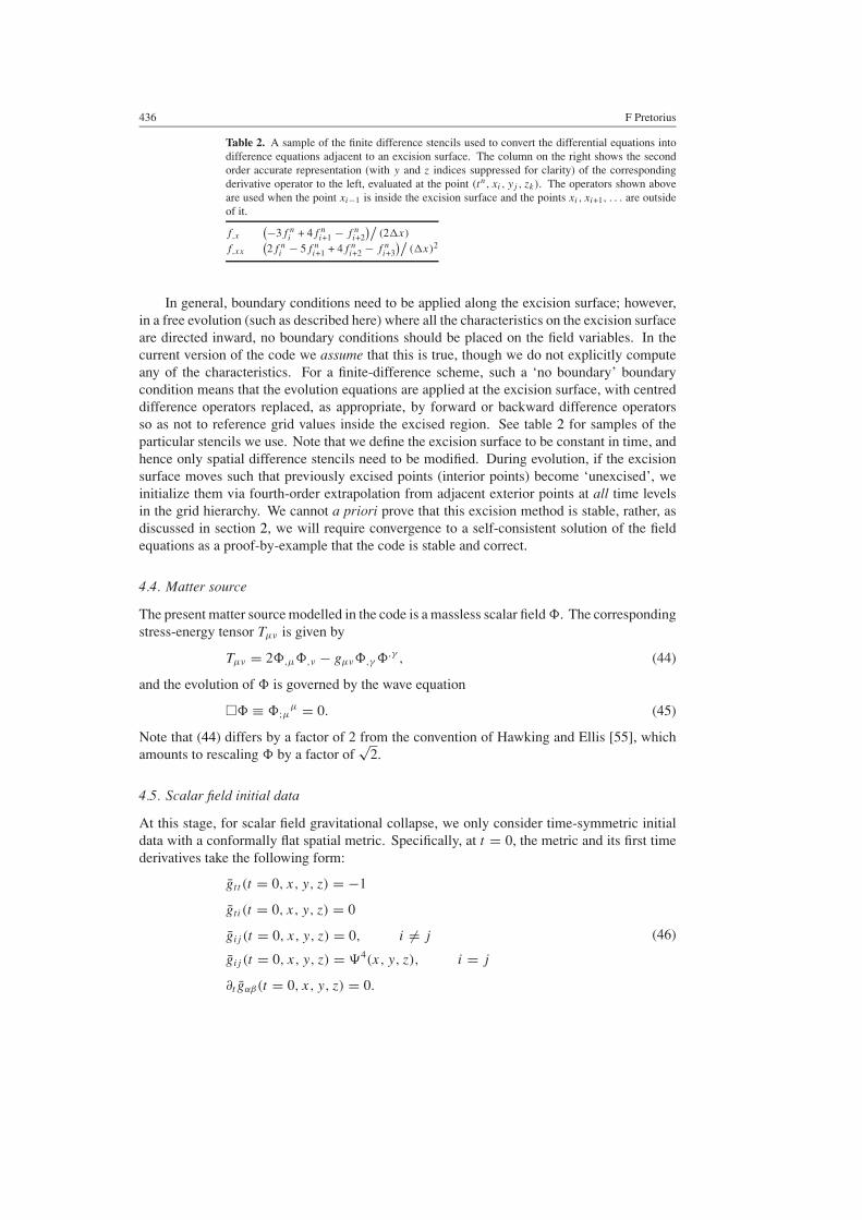
436 F Pretorius

Table 2. A sample of the finite difference stencils used to convert the differential equations intodifference equations adjacent to an excision surface. The column on the right shows the secondorder accurate representation (with y and z indices suppressed for clarity) of the correspondingderivative operator to the left, evaluated at the point (tn, xi , yj , zk). The operators shown aboveare used when the point xi−1 is inside the excision surface and the points xi , xi+1, . . . are outsideof it.

f,x

(−3f ni + 4f n

i+1 − f ni+2

)/(2�x)

f,xx

(2f n

i − 5f ni+1 + 4f n

i+2 − f ni+3

)/(�x)2

In general, boundary conditions need to be applied along the excision surface; however,in a free evolution (such as described here) where all the characteristics on the excision surfaceare directed inward, no boundary conditions should be placed on the field variables. In thecurrent version of the code we assume that this is true, though we do not explicitly computeany of the characteristics. For a finite-difference scheme, such a ‘no boundary’ boundarycondition means that the evolution equations are applied at the excision surface, with centreddifference operators replaced, as appropriate, by forward or backward difference operatorsso as not to reference grid values inside the excised region. See table 2 for samples of theparticular stencils we use. Note that we define the excision surface to be constant in time, andhence only spatial difference stencils need to be modified. During evolution, if the excisionsurface moves such that previously excised points (interior points) become ‘unexcised’, weinitialize them via fourth-order extrapolation from adjacent exterior points at all time levelsin the grid hierarchy. We cannot a priori prove that this excision method is stable, rather, asdiscussed in section 2, we will require convergence to a self-consistent solution of the fieldequations as a proof-by-example that the code is stable and correct.

4.4. Matter source

The present matter source modelled in the code is a massless scalar field . The correspondingstress-energy tensor Tµν is given by

Tµν = 2 ,µ ,ν − gµν ,γ ,γ , (44)

and the evolution of is governed by the wave equation

� ≡ ;µµ = 0. (45)

Note that (44) differs by a factor of 2 from the convention of Hawking and Ellis [55], whichamounts to rescaling by a factor of

√2.

4.5. Scalar field initial data

At this stage, for scalar field gravitational collapse, we only consider time-symmetric initialdata with a conformally flat spatial metric. Specifically, at t = 0, the metric and its first timederivatives take the following form:

gtt (t = 0, x, y, z) = −1

gti (t = 0, x, y, z) = 0

gij (t = 0, x, y, z) = 0, i �= j

gij (t = 0, x, y, z) = �4(x, y, z), i = j

∂t gαβ(t = 0, x, y, z) = 0.

(46)

Numerical relativity using a generalized harmonic decomposition 437

The scalar field is thus the source of all non-trivial geometry at t = 0, and we initialize it as asum of Gaussian-like functions of the following form:

(t = 0, x, y, z) =∑

i

f i(x, y, z), ∂t (t = 0, x, y, z) = 0, (47)

with

f i(x, y, z) = Ai exp(−[ρi(x, y, z)/�i]2),

ρi(x, y, z) = {[1 − εi

x2][x(x) − xi

0

]2+

[1 − εi

y2][y(y) − yi

0

]2+

[1 − εi

z2][z(z) − zi

0

]2}1/2,

(48)

where Ai,�i, εi

x, εiy, ε

iz, x

i0, y

i0 and zi

0 are constants, and x(x), y(y) and z(z) are given by (34).In (46), �(x, y, z) is solved for using the Hamiltonian constraint (13) equation, using an

adaptive multigrid routine as discussed in [51, 52]. Note however that some complicationsdo arise when attempting to solve an elliptic equation in compactified coordinates usingmultigrid; we will briefly discuss these issues in section 4.5.1. The momentum constraints (14)are trivially satisfied with the above initial conditions. Once the constraints have been solved,we initialize the source functions H α(t = 0, x, y, z) using (37) and (7).

With a three time level evolution scheme, the past time level at t = −�t needs to beinitialized as well. To obtain second-order accurate convergence of the solution at late times,the past time level needs to be consistent with the initial data to within �t2. In the code wehave implemented a couple of methods to achieve this; the first is to use a Taylor expansionalong with the equations of motion, the second is to evolve backward in time to t = −�t

with a smaller time step. The first method works as follows [56]. For any one of the evolvedgrid functions f n

ijk the past time level n = −1 is initialized to second-order accuracy using aTaylor expansion about t = 0

f −1ijk = f 0

ijk − f ′0ijk�t + f ′′0

ijk

�t2

2, (49)

where f ′0ijk is the first time derivative of f (t, x, y, z) at t = 0 (from the initial data), and f ′′0

ijk

is the second time derivative of f (t, x, y, z) at t = 0, evaluated by substituting the initial datainto the relevant equations of motion (9, 45) and solving for ∂t∂tf . For the second method,the past time level is only initialized to first order using f 0

ijk and f ′0ijk , however with a smaller

time step �ts ≈ �t2. These initial data are then evolved backward in time until t = −�t ,and the solution obtained there is used to initialize the past time level for the actual evolution.

4.5.1. Multigrid in a compactified coordinate system. Standard geometric multigrid (MG)methods that use pointwise relaxation as a smoother (as we do) are only efficient when thesize of the coefficient functions multiplying each of the principal parts of the elliptic operatorare of comparable size [57]. This is the not the case near i0 in our compactified coordinatesystem. To illustrate, consider the form of the spatial Laplacian ∇2 using the coordinates ofsection 4.2 in flatspace

∇2 = 4

π2

(cos4(πx/2)

∂2

∂x2+ cos4(πy/2)

∂2

∂y2+ cos4(πz/2)

∂2

∂z2

)+ · · · , (50)

where the . . . denote lower-order terms. Note that near any one of the outer boundariesxi = ±1 the corresponding coefficient of the second derivative term goes to zero. We have notsolved the issue of multigrid inefficiency in this part of the domain; however, if we use scalarfield initial data of compact support in a sufficiently small region about (x, y, z) = (0, 0, 0),then we find that the fine-grid relaxation performed within MG is adequate in obtaining a

438 F Pretorius

solution of sufficient accuracy near i0 (for � will then go as 1 + O(1/r), and the initial guessof � = 1 is close enough to the solution that relatively few relaxation sweeps are needed).

A more serious problem is that relaxation using standard centred differenceapproximations for first derivatives is unstable near i0. A partial solution to this problemis to use the following 4-way corner-averaged difference operator at the grid point (i, j, k)

(shown here for the x derivative; the other first difference operators are similarly modified)

f,x = (fi+1,j+1,k+1 − fi−1,j+1,k+1)/(8�x) + (fi+1,j+1,k−1 − fi−1,j+1,k−1)/(8�x)

+ (fi+1,j−1,k+1 − fi−1,j−1,k+1)/(8�x)

+ (fi+1,j−1,k−1 − fi−1,j−1,k−1)/(8�x) + O(�x2). (51)

In the limit where the mesh spacing goes to zero in the vicinity of xi = ±1, even thismodification exhibits relaxation instabilities for initial data that are not sufficiently compactabout r = 0. However, this is not a problem for the kinds of physical system we plan to usethe code for, as all the interesting dynamics will be confined to a small region about r = 0,and this will be part of the hierarchy with high resolution.

4.6. Exact Schwarzschild black-hole initial data

For some of the tests described here we use analytic initial data from a Schwarzschildblack-hole solution in Painleve–Gullstrand-like (PG) coordinates. The non-compactifiedcomponents of the metric are

ds2 = −(

1 − 2M

r

)dt2 + dx2 + dy2 + dz2 +

2√

2M

r3/2[x dx + y dy + z dz] dt, (52)

where r ≡√

x2 + y2 + z2 and M is the mass of the black hole. This (with appropriate spatialcompactification) gives initial data for the metric at t = 0, and is also used to evaluate (7) forthe initial values of the source functions.

4.7. Efficient simulation of axisymmetric spacetimes

In this section a variant of the ‘symmetry without symmetry’, or cartoon method [32] forefficient evolution of an axisymmetric spacetime with a Cartesian-based three-dimensionalcode is described. The advantages to the approach presented here are that no interpolation isever performed, the axisymmetric grid structure is a two-dimensional slice of the Cartesiangrid, rather than a thin three-dimensional slab, and the method is not specific to finite differencebased codes, so can readily be applied to a spectral code, for instance. Having the grid structurebe two-dimensional is helpful in that it allows easy integration of the code with standardadaptive mesh refinement (AMR) packages. The reason is as follows. In the original cartoonalgorithm, the third, thin dimension is one finite-difference stencil-width thick. However,most AMR algorithms can only refine a given volume of a grid, which would increase thewidth of the slab-dimension on finer levels, and thereby reduce the efficiency of the cartoonmethod. Of course the AMR algorithm could be modified to deal with such a situation;however by using a two-dimensional grid structure one avoids this problem altogether. Notealso that the purpose of the algorithm presented here is merely to provide an efficient wayto simulate axisymmetric spacetimes with a Cartesian code, and not to address any issues ofaxis stability in axisymmetric codes, which was one of the original motivations behind thecartoon. Some recent work [34] has suggested that the standard cartoon algorithm may not bestable. Here we deal with the axis by applying appropriate regularity conditions and numericaldissipation, which has proven to be an effective method for dealing with the axial singularity

Numerical relativity using a generalized harmonic decomposition 439

in axisymmetric codes [35, 36] (note also that in some cases stability in axisymmetric codescan be obtained by constructing schemes with a conserved discrete energy, using operatorsthat satisfy summation by parts—see for example [37]).

The idea behind our modified cartoon algorithm is as follows. In a d-dimensionalaxisymmetric spacetime we have an azimuthal Killing vector ξµ, hence the metric gµν and thescalar-field matter source satisfy

Lξ gµν = 0, Lξ = 0. (53)

What these equations imply is that all non-trivial structure of the metric and scalar field areencoded within a (d − 1)-dimensional sub-manifold S of the spacetime, as long as ξµ isnowhere tangent to S. Therefore, one only needs to solve the field equations on S, and (53)can be used to extend the solution throughout the spacetime. In a numerical evolution, itmakes most sense to have S coincide with a constant coordinate hypersurface, which we setto z = 0 for concreteness. We then choose coordinates such that ξµ has the explicit form (inuncompactified coordinates),

ξµ = y

(∂

∂z

)µ

− z

(∂

∂y

)µ

, (54)

which implies that ξµ is orthogonal to z = 0, and the axis of symmetry runs along the x

direction and is centred at y = 0.8 To solve the field equations on z = 0 requires first andsecond derivatives of metric variables both within the hypersurface z = 0, and orthogonal toit in the z direction. To calculate z derivatives the original cartoon method effectively extendsthe solution using (53) to a sufficient number of grid points above and below z = 0, so thatthe usual finite-difference stencils can be used to calculate z derivatives. The approach takenhere is to substitute the explicit form of the Killing vector (54) into the definition (53), anduse the resulting expression to evaluate the z gradients directly. In other words, the samenumerical method is used to solve equations as outlined in section 4.1; however instead ofcalculating z derivatives using finite-difference approximation, the z derivatives are replacedwith appropriate combinations of x and y gradients. In appendix A we list the results ofthis calculation for all relevant gradients of the metric in compactified coordinates; here weillustrate the technique for the simpler case of the scalar field .

Evaluating (53) for using (54), we obtain

∂

∂z= z

y

∂

∂y. (55)

Taking the z derivative of this equation, and replacing any z gradients of appearing on theright-hand side with (55), gives

∂2

∂z2= 1

y

∂

∂y+

z2

y2

(− 1

y

∂

∂y+

∂2

∂y2

). (56)

Evaluating these equations at z = 0 gives

∂

∂z

∣∣∣∣z=0

= 0,∂2

∂z2

∣∣∣∣z=0

= 1

y

∂

∂y. (57)

All other mixed second derivatives of involving z are zero.One thing to note from equation (57) is that the axis y = 0 is singular. Therefore a

regularity condition needs to be applied there, which can easily be seen from (57) to be∂ /∂y = 0 at y = 0.

8 In other words, (54) is merely the Cartesian form of (∂/∂φ)µ, where φ is a standard azimuthal coordinate with theaxis of symmetry coincident with the x axis.

440 F Pretorius

5. Preliminary results

In this section we present results from several test simulations demonstrating certain aspectsof the code. Significantly more work needs to be done before the code may be able to producenew physical results; however the current simulations suggest that the generalized harmonicdecomposition could be a viable alternative to the ADM decomposition for many problems ofinterest.

In section 5.1 we show a convergence test of scalar-field evolution in 3D, section 5.2evolves a Schwarzschild black hole in Painleve–Gullstrand coordinates, and section 5.3demonstrates gravitational collapse of scalar-field initial data to a Schwarzschild black hole.

5.1. Convergence test

For a 3D convergence test we used the following initial conditions for (47), which describesthree prolate spheroids slightly offset from one another so that there is no spatial symmetry inthe problem:

A1 = 0.034, A2 = 0.033, A3 = 0.033

�1 = 0.1, �2 = 0.1, �3 = 0.1(x1

0 , y10 , z1

0

) = (0.025, 0, 0),(x2

0 , y20 , z2

0

) = (0,−0.025,−0.025),(x3

0 , y30 , z3

0

) = (−0.025.025, 0.025)

ε1x = 0.1, ε2

y = 0.1, ε3z = 0.1

(58)

and all other initial data parameters for are zero. With these parameters the ADM mass ofthe spacetime is roughly 0.005, so the initial distribution of energy is concentrated in a radiusabout ten times larger than its effective Schwarzschild radius. For the Ht coordinate conditionwe used a slightly modified version of (26), where we eliminated the coupling (through thenormal nµ) to Hi and added an arbitrary power n of α in the denominator:

�Ht = −κt (t)α − α0

αn+ ξt (t)Ht ,µnµ, (59)

where κt (t) = κ0q(t), ξt (t) = ξ0q(t) and q(t) is given by

q(t) =(

t

t1

)3[

6

(t

t1

)2

− 15t

t1+ 10

], 0 � t � t1

= 0, elsewhere. (60)

q(t) provides a smooth (twice differentiable) transition from 0 at t = 0 to 1 at t = t1, andmakes the evolution of the source functions consistent with the choice of time-symmetricinitial data. We evolve H i to zero using a version of (16) with Hi replaced by H i , andκi(t) = κ0q(t). For this particular simulation we had κ0 = 50, ξ0 = 10, n = 3, t1 = 1/10 andα0 = 1.

A convergence test involves running a given simulation at several different resolutions,and comparing the results to ensure that the solution of the finite-difference equations isconverging to a solution of the partial differential equations. We ran three simulations ofdiffering resolution. The coarsest resolution run had a base grid size of 173, and we specifieda value for the maximum desired truncation error so that up to five additional levels of 2 : 1refinement were used, giving an effective finest resolution of 5133—see figure 2 for a depictionof the mesh structure at two times during the simulation. We used a Courant factor of 0.25

Numerical relativity using a generalized harmonic decomposition 441

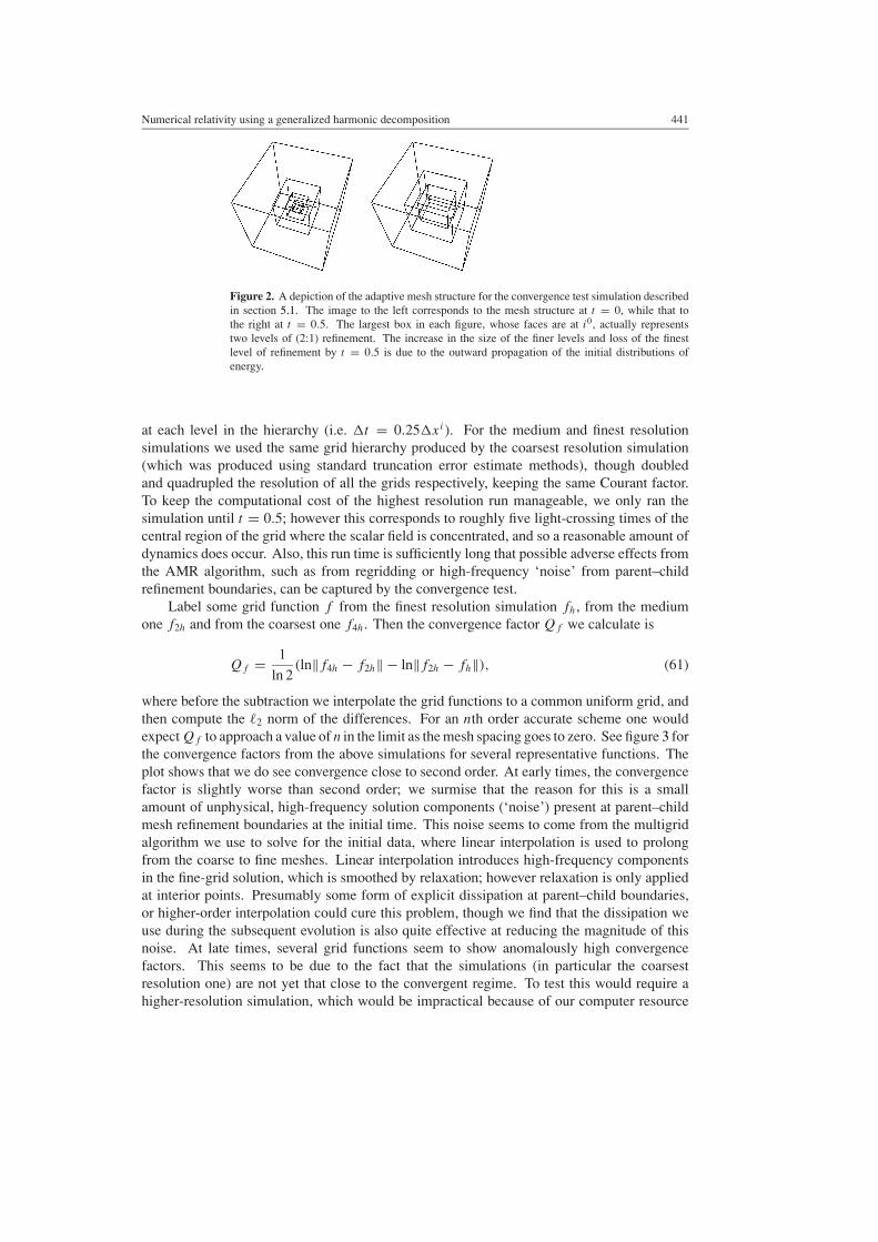
Figure 2. A depiction of the adaptive mesh structure for the convergence test simulation describedin section 5.1. The image to the left corresponds to the mesh structure at t = 0, while that tothe right at t = 0.5. The largest box in each figure, whose faces are at i0, actually representstwo levels of (2:1) refinement. The increase in the size of the finer levels and loss of the finestlevel of refinement by t = 0.5 is due to the outward propagation of the initial distributions ofenergy.

at each level in the hierarchy (i.e. �t = 0.25�xi). For the medium and finest resolutionsimulations we used the same grid hierarchy produced by the coarsest resolution simulation(which was produced using standard truncation error estimate methods), though doubledand quadrupled the resolution of all the grids respectively, keeping the same Courant factor.To keep the computational cost of the highest resolution run manageable, we only ran thesimulation until t = 0.5; however this corresponds to roughly five light-crossing times of thecentral region of the grid where the scalar field is concentrated, and so a reasonable amount ofdynamics does occur. Also, this run time is sufficiently long that possible adverse effects fromthe AMR algorithm, such as from regridding or high-frequency ‘noise’ from parent–childrefinement boundaries, can be captured by the convergence test.

Label some grid function f from the finest resolution simulation fh, from the mediumone f2h and from the coarsest one f4h. Then the convergence factor Qf we calculate is

Qf = 1

ln 2(ln‖f4h − f2h‖ − ln‖f2h − fh‖), (61)

where before the subtraction we interpolate the grid functions to a common uniform grid, andthen compute the �2 norm of the differences. For an nth order accurate scheme one wouldexpect Qf to approach a value of n in the limit as the mesh spacing goes to zero. See figure 3 forthe convergence factors from the above simulations for several representative functions. Theplot shows that we do see convergence close to second order. At early times, the convergencefactor is slightly worse than second order; we surmise that the reason for this is a smallamount of unphysical, high-frequency solution components (‘noise’) present at parent–childmesh refinement boundaries at the initial time. This noise seems to come from the multigridalgorithm we use to solve for the initial data, where linear interpolation is used to prolongfrom the coarse to fine meshes. Linear interpolation introduces high-frequency componentsin the fine-grid solution, which is smoothed by relaxation; however relaxation is only appliedat interior points. Presumably some form of explicit dissipation at parent–child boundaries,or higher-order interpolation could cure this problem, though we find that the dissipation weuse during the subsequent evolution is also quite effective at reducing the magnitude of thisnoise. At late times, several grid functions seem to show anomalously high convergencefactors. This seems to be due to the fact that the simulations (in particular the coarsestresolution one) are not yet that close to the convergent regime. To test this would require ahigher-resolution simulation, which would be impractical because of our computer resource

442 F Pretorius

Figure 3. Convergence factors (61) for representative grid functions from the simulation describedin section 5.1. The points denote the times when Q was calculated, and correspond to times whenthe entire grid hierarchy was in sync. Note that we only show Qgxx at t = 0, as all the otherfunctions are exactly known then, and hence Q is ill defined. This plot shows that the solution isclose to second-order convergent, with some caveats discussed in the text.

limitations9. However, by looking at an independent residual of the Einstein equations, asdescribed next, we can already see the trend towards second-order convergence using onlythree simulations.

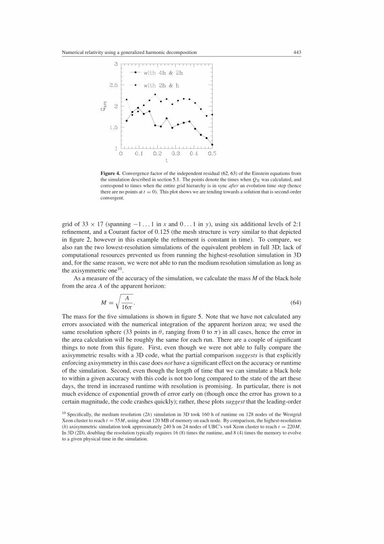
To check that we are solving the Einstein equations we compute an independent residualRαβ of (1):

Rαβ = Rαβ − 4π(2πTαβ − gαβT ). (62)

After discretizing the ten residuals Rαβ using the finite-difference stencils described in thepreceding section, we compute the residual grid function R at each grid point as the infinitynorm over the ten residuals. Note that we compute (62) without reference to the sourcefunctions, using only the compactified metric elements and scalar field. Since we know thatR should converge to zero in the limit, it is sufficient to compute its convergence factor usingtwo resolutions, for example

QR = 1

ln 2(ln‖R2h‖ − ln‖Rh‖). (63)

Figure 4 shows QR computed using both [R2h,Rh] and [R4h,R2h]. This plot shows that weare tending towards second-order convergence as the resolution is increased.

5.2. Schwarzschild black-hole evolution

In this section we briefly show how well the current code can evolve a Schwarzschild blackhole in Painleve–Gullstrand coordinates. The analytic solution is used for initial conditions asdescribed in section 4.6, with M = 0.05, and using (15) to keep the source functions frozenin during evolution. A (‘lego’) spherical excision region of radius 1.2M was used. We ranthree axisymmetric simulations, each with identical grid hierarchy, though successively higherresolution as described in the previous section. The lowest-resolution simulation had a base

9 Alternatively, we can choose initial data that are better resolved on the coarsest grid; however, the kind of resolutionwe have here is more representative of the resolution we will be able to achieve in the near future with the computerpower we have access to, and so we think this is a fair test of the code.

Numerical relativity using a generalized harmonic decomposition 443

Figure 4. Convergence factor of the independent residual (62, 63) of the Einstein equations fromthe simulation described in section 5.1. The points denote the times when QR was calculated, andcorrespond to times when the entire grid hierarchy is in sync after an evolution time step (hencethere are no points at t = 0). This plot shows we are tending towards a solution that is second-orderconvergent.

grid of 33 × 17 (spanning −1 . . . 1 in x and 0 . . . 1 in y), using six additional levels of 2:1refinement, and a Courant factor of 0.125 (the mesh structure is very similar to that depictedin figure 2, however in this example the refinement is constant in time). To compare, wealso ran the two lowest-resolution simulations of the equivalent problem in full 3D; lack ofcomputational resources prevented us from running the highest-resolution simulation in 3Dand, for the same reason, we were not able to run the medium resolution simulation as long asthe axisymmetric one10.

As a measure of the accuracy of the simulation, we calculate the mass M of the black holefrom the area A of the apparent horizon:

M =√

A

16π. (64)

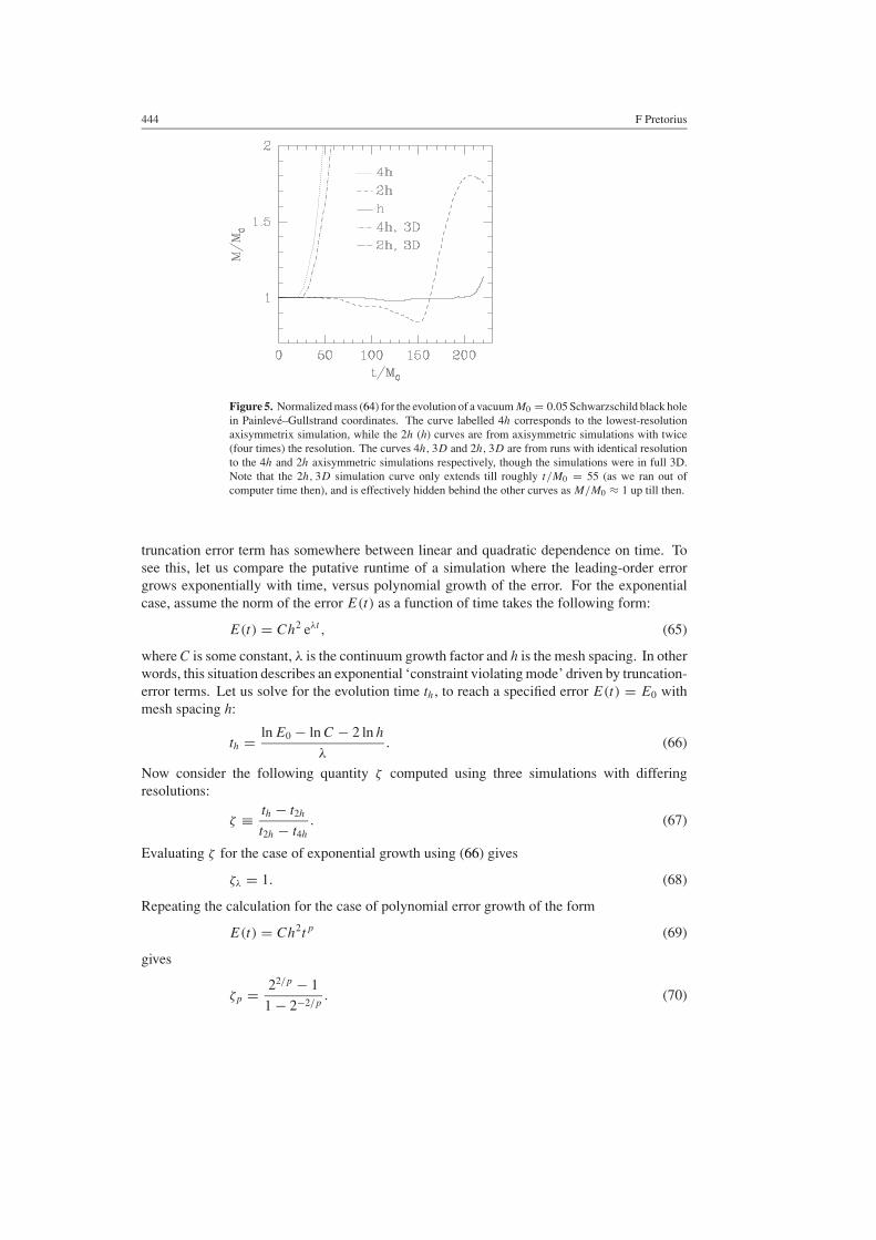
The mass for the five simulations is shown in figure 5. Note that we have not calculated anyerrors associated with the numerical integration of the apparent horizon area; we used thesame resolution sphere (33 points in θ , ranging from 0 to π ) in all cases, hence the error inthe area calculation will be roughly the same for each run. There are a couple of significantthings to note from this figure. First, even though we were not able to fully compare theaxisymmetric results with a 3D code, what the partial comparison suggests is that explicitlyenforcing axisymmetry in this case does not have a significant effect on the accuracy or runtimeof the simulation. Second, even though the length of time that we can simulate a black holeto within a given accuracy with this code is not too long compared to the state of the art thesedays, the trend in increased runtime with resolution is promising. In particular, there is notmuch evidence of exponential growth of error early on (though once the error has grown to acertain magnitude, the code crashes quickly); rather, these plots suggest that the leading-order

10 Specifically, the medium resolution (2h) simulation in 3D took 160 h of runtime on 128 nodes of the WestgridXeon cluster to reach t = 55M , using about 120 MB of memory on each node. By comparison, the highest-resolution(h) axisymmetric simulation took approximately 240 h on 24 nodes of UBC’s vn4 Xeon cluster to reach t = 220M .In 3D (2D), doubling the resolution typically requires 16 (8) times the runtime, and 8 (4) times the memory to evolveto a given physical time in the simulation.

444 F Pretorius

Figure 5. Normalized mass (64) for the evolution of a vacuum M0 = 0.05 Schwarzschild black holein Painleve–Gullstrand coordinates. The curve labelled 4h corresponds to the lowest-resolutionaxisymmetrix simulation, while the 2h (h) curves are from axisymmetric simulations with twice(four times) the resolution. The curves 4h, 3D and 2h, 3D are from runs with identical resolutionto the 4h and 2h axisymmetric simulations respectively, though the simulations were in full 3D.Note that the 2h, 3D simulation curve only extends till roughly t/M0 = 55 (as we ran out ofcomputer time then), and is effectively hidden behind the other curves as M/M0 ≈ 1 up till then.

truncation error term has somewhere between linear and quadratic dependence on time. Tosee this, let us compare the putative runtime of a simulation where the leading-order errorgrows exponentially with time, versus polynomial growth of the error. For the exponentialcase, assume the norm of the error E(t) as a function of time takes the following form:

E(t) = Ch2 eλt , (65)

where C is some constant, λ is the continuum growth factor and h is the mesh spacing. In otherwords, this situation describes an exponential ‘constraint violating mode’ driven by truncation-error terms. Let us solve for the evolution time th, to reach a specified error E(t) = E0 withmesh spacing h:

th = ln E0 − ln C − 2 ln h

λ. (66)

Now consider the following quantity ζ computed using three simulations with differingresolutions:

ζ ≡ th − t2h

t2h − t4h

. (67)

Evaluating ζ for the case of exponential growth using (66) gives

ζλ = 1. (68)

Repeating the calculation for the case of polynomial error growth of the form

E(t) = Ch2tp (69)

gives

ζp = 22/p − 1

1 − 2−2/p. (70)

Numerical relativity using a generalized harmonic decomposition 445

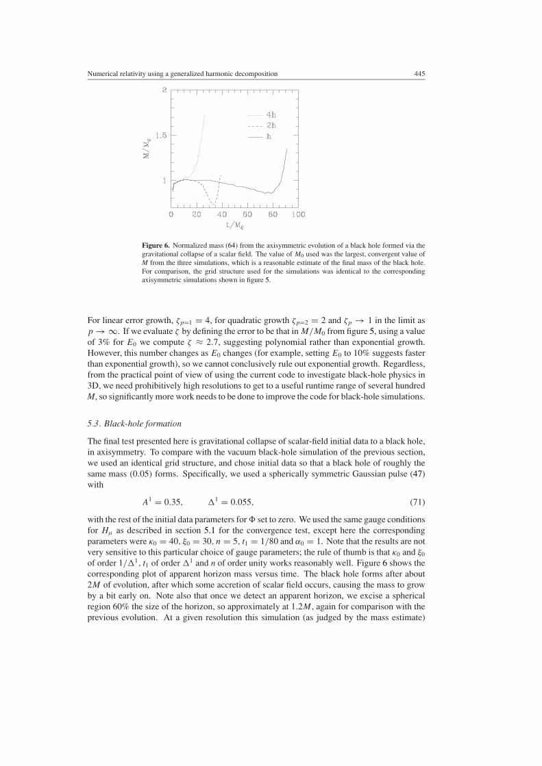
Figure 6. Normalized mass (64) from the axisymmetric evolution of a black hole formed via thegravitational collapse of a scalar field. The value of M0 used was the largest, convergent value ofM from the three simulations, which is a reasonable estimate of the final mass of the black hole.For comparison, the grid structure used for the simulations was identical to the correspondingaxisymmetric simulations shown in figure 5.

For linear error growth, ζp=1 = 4, for quadratic growth ζp=2 = 2 and ζp → 1 in the limit asp → ∞. If we evaluate ζ by defining the error to be that in M/M0 from figure 5, using a valueof 3% for E0 we compute ζ ≈ 2.7, suggesting polynomial rather than exponential growth.However, this number changes as E0 changes (for example, setting E0 to 10% suggests fasterthan exponential growth), so we cannot conclusively rule out exponential growth. Regardless,from the practical point of view of using the current code to investigate black-hole physics in3D, we need prohibitively high resolutions to get to a useful runtime range of several hundredM, so significantly more work needs to be done to improve the code for black-hole simulations.

5.3. Black-hole formation

The final test presented here is gravitational collapse of scalar-field initial data to a black hole,in axisymmetry. To compare with the vacuum black-hole simulation of the previous section,we used an identical grid structure, and chose initial data so that a black hole of roughly thesame mass (0.05) forms. Specifically, we used a spherically symmetric Gaussian pulse (47)with

A1 = 0.35, �1 = 0.055, (71)

with the rest of the initial data parameters for set to zero. We used the same gauge conditionsfor Hµ as described in section 5.1 for the convergence test, except here the correspondingparameters were κ0 = 40, ξ0 = 30, n = 5, t1 = 1/80 and α0 = 1. Note that the results are notvery sensitive to this particular choice of gauge parameters; the rule of thumb is that κ0 and ξ0

of order 1/�1, t1 of order �1 and n of order unity works reasonably well. Figure 6 shows thecorresponding plot of apparent horizon mass versus time. The black hole forms after about2M of evolution, after which some accretion of scalar field occurs, causing the mass to growby a bit early on. Note also that once we detect an apparent horizon, we excise a sphericalregion 60% the size of the horizon, so approximately at 1.2M , again for comparison with theprevious evolution. At a given resolution this simulation (as judged by the mass estimate)

446 F Pretorius

has less accuracy compared to the corresponding vacuum simulation; however the trend ofincreased accuracy with increased resolution is roughly the same.

6. Conclusion

We have described a new computational scheme for numerically solving the Einstein equationsbased upon generalized harmonic coordinates. This extends the earlier work of Garfinkle [20],and in some respects is similar to the direction pursued by Szilagyi and Winicour [21]. Someof the topics covered included suggestions for imposing dynamical gauge conditions, a newtechnique of implementing the cartoon method [32] for simulating axisymmetric spacetimeswith a Cartesian code, a direct discretization scheme for second-order-in-space-and-timepartial differential equations, and the use of a spatially compactified coordinate system. Oneattractive feature of harmonic evolution is that the principal part of the Einstein equationsreduce to wave equations for each metric element. This, together with the use of a second-order discretization scheme, keeps the number of variables and constraint equations to aminimum, and the hope is that this will make it easier to achieve stable evolution. The use ofa spatially compactified domain allows one to impose correct asymptotic boundary conditionsfor the simulation, and thus we automatically have constraint preserving boundary conditions.The advantage of our cartoon method over the original is that no interpolation is needed,and the simulation is performed on a 2D slice of the spacetime, thus simplifying the processof incorporating the code into an adaptive mesh refinement framework. Furthermore, thetechnique is not particular to finite-difference codes, and can be used with spectral methods,for instance.

Preliminary test simulations of black-hole spacetimes suggest that this scheme holdspromise for being applicable to many problems of interest, including the binary black-holeproblem, black-hole–matter interactions and critical gravitational collapse. However, a lot ofresearch still needs to be done, at both the analytical and numerical levels, before this schememay produce new physical results. In particular, it would be useful to analyse the mathematicalwell-posedness of the fully discrete system, including a variety of possible gauge evolutionequations. The majority of techniques for analysing hyperbolic systems require reduction tofirst-order form (recently similar techniques have been developed for second order in space,first order in time systems [58–60]; also, in [61] the BSSN system is analysed by convertinginto first-order form; however the constraints introduced by this reduction are shown to obey aclosed evolution system that is independent of the other constraints, implying that the originalsecond-order system is well-posed). At the numerical level, a broader class of initial conditionsneeds to be explored, such as black-hole–matter interactions and black-hole collisions. Thisis of course one of the primary long-term goals of the code; however early tests indicatethat a significant number of adjustments and improvements (to dissipation and extrapolationoperators, for example) may be needed, in addition to more sophisticated gauge conditionsthan discussed here, before such scenarios could be simulated with sufficient accuracy andlength of time for new results to be obtained.

Acknowledgments

I would like to thank Matthew Choptuik for many stimulating discussions about the workpresented here. I gratefully acknowledge research support from NSF PHY-0099568, NSFPHY-0244906 and Caltech’s Richard Chase Tolman Fund. Simulations were performed onUBC’s vn cluster, (supported by CFI and BCKDF), and the Westgrid cluster (supported byCFI, ASRI and BCKDF).

Numerical relativity using a generalized harmonic decomposition 447

Appendix A. Evolution of axisymmetric spacetimes

As described in section 4.7, we can efficiently simulate axisymmetric spacetimes along asingle z = 0 slice of the spacetime by replacing all z gradients in the field and matter evolutionequations with appropriate x and y gradients, as dictated by (53). Here we list the equationsfor gradients of the regular components of the metric gµν and scalar field with respectto the compactified coordinates (section 4.2), and give the corresponding on-axis regularityconditions.

The first z derivatives are

∂zgtt |z=0 = 0, ∂zgtx |z=0 = 0

∂zgty |z=0 = −gt z(π/2y), ∂zgt z|z=0 = gt y (π/2y)

∂zgxx |z=0 = 0, ∂zgxy |z=0 = −gxz(π/2y)

∂zgxz|z=0 = gxy (π/2y), ∂zgyy |z=0 = −gyz(π/y)

∂zgyz|z=0 = (gyy − gzz)(π/2y), ∂zgzz|z=0 = gyz(π/y)

∂z |z=0 = 0.

(A1)

Mixed z–t, z–x and z–y second derivatives are calculated by taking the appropriate derivativeof (A1). Second derivatives with respect to z are computed as follows:

∂z∂zgαβ |z=0 = π

2

(∂ygαβ

y(1 + y2)+

πCαβ

2y2

), ∂z∂z |z=0 = π∂y

2y(1 + y2)(A2)

where the coefficients Cαβ are

Ctt = 0, Ctx = 0

Cty = −gt y , Ctz = −gt z

Cxx = 0, Cxy = −gxy

Cxz = −gxz, Cyy = 2(gzz − gyy )

Cyz = −4gyz, Czz = 2(gyy − gzz).

(A3)

The on-axis regularity conditions are

∂ygtt |y=0 = 0, ∂ygtx |y=0 = 0

gt y |y=0 = 0, gt z|y=0 = 0

∂ygxx |y=0 = 0, gxy |y=0 = 0

gxz|y=0 = 0, ∂ygyy |y=0 = 0

∂ygyz|y=0 = 0, ∂ygzz|y=0 = 0

∂y |y=0 = 0, gyy |y=0 = gzz|y=0.

(A4)

To compute the z gradients and regularity conditions for the source functions in the code,we simply substitute the results from the calculation for the metric into the definition of thesource functions (7), (37).

Appendix B. Stability analysis of a second order in space and time evolution scheme

Here we give a von Neumann-like stability analysis of the one-dimensional flat space waveequation using the discretization scheme described in section 4. Second order in time schemes

448 F Pretorius

for the wave equation are not very common in the literature, so the example given here is todemonstrate that the method is inherently stable, ignoring the complications of boundaries,excision, non-constant coefficients and nonlinear lower-order terms of the full problem (theanalysis of which is beyond the scope of this paper). Even though dissipation is not needed inthis example, we add it as applied in the code to demonstrate how it works.

The model wave equation for (x, t) is

,tt − ,xx = 0. (B1)

Discretization of this equation using the stencils in table 1 gives

n+1j − 2 n

j + n−1j − λ2

( n

j+1 − 2 nj + n

j−1

) = 0, (B2)

where nj ≡ (x = j�x, t = n�t) and λ ≡ �t/�x is the Courant factor. This immediately

gives an explicit update scheme for the unknown n+1 given information at two past timelevels, n, n−1:

n+1j = 2 n

j − n−1j + λ2( n

j+1 − 2 nj + n

j−1

)(B3)

(note that the iterative relaxation method described in section 4 gives exactly the same updatescheme in this case). It is mathematically simpler to analyse this equation using an equivalenttwo time level scheme by introducing the variable

�nj ≡ n−1

j , (B4)

after which (B3) becomes

n+1j = 2 n

j − �nj + λ2

( n

j+1 − 2 nj + n

j−1

), �n+1

j = nj . (B5)

As (B5) is linear with constant coefficients, we can completely characterize its stabilityproperties by analysing the evolution of individual Fourier modes of the form c(t) eikx . To thisend, let

(x, t) ≡ a(t) eikx (B6)

�(x, t) ≡ b(t) eikx . (B7)

Substituting this into (B5) gives

an+1 = 2an − bn − 4λ2ξ 2an, bn+1 = an, (B8)

where

ξ ≡ sin(k�x/2), (B9)

and we have used the identity −4 sin2(k�x/2) = e−ik�x − 2 + eik�x . Note that the smallestwavelength that can be represented on a numerical grid is 2�x (the Nyquist limit), whichcorresponds to a largest possible wave number k = π/�x, hence ξ ranges from 0 to 1.

As described in section 4.1.1, we apply numerical dissipation to all past time levelvariables, prior to the update step, by first calculating the high-frequency component of thefunction using (30), and then subtracting it from the function via (31). For a grid functionf n

j = cn eikxj , the high-frequency component ηnj is defined as

ηnj = 1

16

(f n

j−2 − 4f nj−1 + 6f n

j − 4f nj+1 + f n

j+2

)= f n

j ξ 4, (B10)

and filtering amounts to modifying f nj as follows:

f nj → f n

j − εηnj

= f nj (1 − εξ 4)

= εf nj , (B11)

Numerical relativity using a generalized harmonic decomposition 449

where ε ≡ 1 − εξ 4. As ξ ∈ [0. . . . 1] and ε ∈ [0 . . . 1], ε ∈ [0 . . . 1]. With this form ofdissipation (which is linear, and hence fits into the Fourier analysis of the evolution scheme)applied to both n

j and �nj , (B8) becomes

an+1 = ε[2an(1 − 2λ2ξ 2) − bn], bn+1 = εan. (B12)

In matrix form, the update step can be written as[a

b

]n+1

= A[a

b

]n

, (B13)

where

A = ε

[2(1 − 2λ2ξ 2) −1

1 0

]. (B14)

The numerical evolution will be stable if the eigenvalues �± of A all lie on or within the unitcircle in the complex plain. A straightforward calculation gives

�± = ε[1 − 2ξ 2λ2 ± i2ξλ√

1 − ξ 2λ2]. (B15)

The expression within the square root of (B15) is strictly non-negative if we require thatλ ∈ [0 . . . 1]. The magnitude of the eigenvalues are

‖�±‖ = ε. (B16)

Hence, for ε � 1 the numerical scheme is stable; in fact, without dissipation (ε = 1) thescheme is inherently stable and non-dissipative.

References

[1] Reula O A 1998 Hyperbolic methods for Einstein’s equations Living Rev. Rel. 1:3[2] Lehner L 2001 Numerical relativity: a review Class. Quantum Grav. 18 R25[3] Nakamura T, Oohara K and Kojima Y 1987 Prog. Theor. Phys. Suppl. 90 1[4] Shibata M and Nakamura T 1995 Evolution of three-dimensional gravitational waves: harmonic slicing case

Phys. Rev. D 52 5428[5] Baumgarte T W and Shapiro S L 1999 Numerical integration of Einstein’s field equations Phys. Rev. D 59

024007[6] Bruegmann B, Tichy W and Jansen N 2004 Numerical simulation of orbiting black holes Phys. Rev. Lett. 92

211101[7] Bishop N T, Gomez R, Husa S, Lehner L and Winicour J 2003 A numerical relativistic model of a massive

particle in orbit near a Schwarzschild black hole Phys. Rev. D 68 084015[8] Anderson M and Matzner R A 2003 Extended lifetime in computational evolution of isolated black holes

Preprint gr-qc/0307055[9] Bonazzola S, Gourgoulhon E, Grandclement P and Novak J 2004 A constrained scheme for Einstein equations

based on Dirac gauge and spherical coordinates Phys. Rev. D 70 104007[10] Holst M, Lindblom L, Owen R, Pfeiffer H P, Scheel M A and Kidder L E 2004 Optimal constraint projection

for hyperbolic evolution systems Phys. Rev. D 70 084017[11] Buchman L T and J M 2003 A hyperbolic tetrad formulation of the Einstein equations for numerical relativity

Phys. Rev. D 67 084017[12] Estabrook F B, Robinson R S and Wahlquist H D 1997 Hyperbolic equations for vacuum gravity using special

orthonormal frames Class. Quantum Grav. 14 1237[13] Buchman L T and Bardeen J M 2003 A hyperbolic tetrad formulation of the Einstein equations for numerical

relativity Phys. Rev. D 67 084017[14] Estabrook F B 2004 Mathematical structure of tetrad equations for numerical relativity Preprint gr-qc/0411029[15] Friedrich H 1981 On the regular and the asymptotic characteristic initial value problem for Einstein’s vacuum

field equations Proc. R. Soc. A 375 169[16] Friedrich H 1981 The asymptotic characteristic initial value problem for Einstein’s vacuum field equations as

an initial value problem for a first-order quasilinear symmetric hyperbolic system Proc. R. Soc. A 378 401

450 F Pretorius

[17] Hubner P 1999 A scheme to numerically evolve data for the conformal Einstein equation Class. Quantum Grav.16 2823

[18] Husa S 2003 Numerical relativity with the conformal field equations Lect. Notes. Phys. 617 159[19] Bruhat Y 1962 The Cauchy problem Gravitation: An Introduction to Current Research ed L Witten (New York:

Wiley)[20] Garfinkle D 2002 Harmonic coordinate method for simulating generic singularities Phys. Rev. D 65 044029[21] Szilagyi B and Winicour J 2003 Well-posed initial-boundary evolution in general relativity Phys. Rev. D 68

041501[22] Bona C, Ledvinka T, Palenzuela C and Zacek M 2003 General-covariant evolution formalism for numerical

relativity Phys. Rev. D 67 104005[23] Calabrese G 2004 Finite differencing second order systems describing black hole spacetimes Preprint gr-

qc/0410062[24] Kreiss H and Ortiz O E 2002 Some mathematical and numerical questions connected with first and second order

time dependent systems of partial differential equations Lect. Notes Phys. 604 359[25] Kelly B, Laguna P, Lockitch K, Pullin J, Schnetter E, Shoemaker D and Tiglio M 2001 A cure for unstable

numerical evolutions of single black holes: adjusting the standard ADM equations Phys. Rev. D 64 084013[26] Shinkai H and Yoneda G 2002 Re-formulating the Einstein equations for stable numerical simulations:

formulation problem in numerical relativity Preprint gr-qc/0209111[27] Tiglio M 2003 Dynamical control of the constraints growth in free evolutions of Einstein’s equations Preprint

gr-qc/0304062[28] Tiglio M, Lehner L and Neilsen D 2004 3D simulations of Einstein’s equations: symmetric hyperbolicity, live

gauges and dynamic control of the constraints Phys. Rev. D 70 104018[29] Lindblom L, Scheel M A, Kidder L E, Pfeiffer H P, Shoemaker D and Teukolsky S A 2004 Controlling the

growth of constraints in hyperbolic evolution systems Phys. Rev. D 69 124025[30] Meier D L 2003 Constrained transport algorithms for numerical relativity. I. Development of a finite difference

scheme Astrophys. J. 595 980[31] Di Bartolo C, Gambini R and Pullin J 2004 Consistent and mimetic discretizations in general relativity Preprint

gr-qc/0404052[32] Alcubierre M, Brandt S, Bruegmann B, Holz D, Seidel E, Takahashi R and Thornburg J 2001 Symmetry without

symmetry: numerical simulation of axisymmetric systems using Cartesian grids Int. J. Mod. Phys. D 10 273[33] Friedrich H 1985 On the hyperbolicity of Einstein’s and other gauge field equations Commun. Math. Phys.

100 525[34] Frauendiener J 2002 On discretizations of axisymmetric systems Phys. Rev. D 66 104027[35] Garfinkle D and Duncan G C 2001 Numerical evolution of Brill waves Phys. Rev. D 63 044011[36] Choptuik M W, Hirschmann E W, Liebling S L and Pretorius F 2003 An axisymmetric gravitational collapse

code Class. Quantum Grav. 20 1857[37] Calabrese G and Neilsen D 2004 Spherical excision for moving black holes and summation by parts for

axisymmetric systems Phys. Rev. D 69 044020[38] Choptuik M W, Lehner L, Olabarrieta I, Petryk R, Pretorius F and Villegas H 2003 Towards the final fate of an

unstable black string Phys. Rev. D 68 044001[39] Thornburg J 1996 Finding apparent horizons in numerical relativity Phys. Rev. D 54 4899[40] Thornburg J 2004 A fast apparent-horizon finder for 3-dimensional Cartesian grids in numerical relativity Class.

Quantum Grav. 21 743[41] Schnetter E 2003 Finding apparent horizons and other two-surfaces of constant expansion Class. Quantum

Grav. 20 4719[42] Cook G B 2000 Initial data for numerical relativity Living Rev. Rel. 3 5[43] Friedrich H 1996 Hyperbolic reductions for Einstein’s equations Class. Quantum Grav. 13 1451[44] York J W 1978 Sources of Gravitational Radiation ed L Smarr (Seattle, WA: Cambridge University Press)[45] Bona C, Masso J, Seidel E and Stela J 1995 New formalism for numerical relativity Phys. Rev. Lett. 75 600[46] Balakrishna J, Daues G, Seidel E, Suen W, Tobias M and Wang E 1996 Coordinate conditions and their

implementation in 3D numerical relativity Class. Quantum Grav. 13 L135[47] Alcubierre M, Bruegmann B, Pollney D, Seidel E and Takahashi R 2001 Black hole excision for dynamic black

holes Phys. Rev. D 64 061501[48] Lindblom L and Scheel M A 2003 Dynamical gauge conditions for the Einstein evolution equations Phys. Rev.

D 67 124005[49] Alcubierre M, Bruegmann B, Diener P, Koppitz M, Pollney D, Seidel E and Takahashi R 2003 Gauge conditions

for long-term numerical black hole evolutions without excision Phys. Rev. D 67 084023[50] Bona C 2004 Private communication

Numerical relativity using a generalized harmonic decomposition 451

[51] Pretorius F and Choptuik M W Adaptive mesh refinement for coupled elliptic-hyperbolic systems, in preparation[52] Pretorius F 2002 Numerical simulations of gravitational collapse PhD Thesis University of British Columbia,

Canada[53] Kreiss H and Oliger J 1973 Methods for the approximate solution of time dependent problems Global

Atmospheric Research Programme (Publications Series No. 10)[54] Calabrese G, Lehner L, Reula O, Sarbach O and Tiglio M 2003 Summation by parts and dissipation for domains

with excised regions Preprint gr-qc/0308007[55] Hawking S W and Ellis G F R 1973 The Large Scale Structure of Space-Time (Cambridge: Cambridge University

Press)[56] Choptuik M W 2003 Private communication[57] Brandt A 1977 Multi-level adaptive solutions to boundary-value problems Math. Comput. 31 330[58] Nagy G, Ortiz O E and Reula O A 2004 Strongly hyperbolic second order Einstein’s evolution equations Phys.

Rev. D 70 044012[59] Gundlach C and Martin-Garcia J M 2004 Symmetric hyperbolic form of systems of second-order evolution

equations subject to constraints Phys. Rev. D 70 044031[60] Gundlach C and Martin-Garcia J M 2004 Symmetric hyperbolicity and consistent boundary conditions for

second-order Einstein equations Phys. Rev. D 70 044032[61] Beyer H and Sarbach O 2004 On the well posedness of the Baumgarte–Shapiro–Shibata–Nakamura formulation

of Einstein’s field equations Phys. Rev. D 70 104004