
LECTURES on
COMPUTATIONAL NUMERICAL
ANALYSIS
of
PARTIAL DIFFERENTIAL EQUATIONS
J. M. McDonough
Departments of Mechanical Engineering and Mathematics
University of Kentucky
c©1985, 2002

ii
Contents
1 Numerical Solution of Elliptic Equations 1
1.1 Background . . . . . . . . . . . . . . . . . . . . . . . . . . . . . . . . . . . . . . . . . 2
1.1.1 Iterative solution of linear systems—an overview . . . . . . . . . . . . . . . . 2
1.1.2 Basic theory of linear iterative methods . . . . . . . . . . . . . . . . . . . . . 5
1.2 Successive Overrelaxation . . . . . . . . . . . . . . . . . . . . . . . . . . . . . . . . . 9
1.2.1 Jacobi iteration . . . . . . . . . . . . . . . . . . . . . . . . . . . . . . . . . . . 9
1.2.2 SOR theory . . . . . . . . . . . . . . . . . . . . . . . . . . . . . . . . . . . . . 13
1.2.3 Some modifications to basic SOR . . . . . . . . . . . . . . . . . . . . . . . . . 19
1.3 Alternating Direction Implicit (ADI) Procedures . . . . . . . . . . . . . . . . . . . . 25
1.3.1 ADI with a single iteration parameter . . . . . . . . . . . . . . . . . . . . . . 26
1.3.2 ADI: the commutative case . . . . . . . . . . . . . . . . . . . . . . . . . . . . 31
1.3.3 ADI: the noncommutative case . . . . . . . . . . . . . . . . . . . . . . . . . . 35
1.4 Incomplete LU Decomposition (ILU) . . . . . . . . . . . . . . . . . . . . . . . . . . . 35
1.4.1 Basic ideas of ILU decomposition . . . . . . . . . . . . . . . . . . . . . . . . . 36
1.4.2 The strongly implicit procedure (SIP) . . . . . . . . . . . . . . . . . . . . . . 37
1.5 Preconditioning . . . . . . . . . . . . . . . . . . . . . . . . . . . . . . . . . . . . . . . 44
1.6 Conjugate Gradient Acceleration . . . . . . . . . . . . . . . . . . . . . . . . . . . . . 46
1.6.1 The method of steepest descent . . . . . . . . . . . . . . . . . . . . . . . . . . 46
1.6.2 Derivation of the conjugate gradient method . . . . . . . . . . . . . . . . . . 48
1.6.3 Relationship of CG to other methods . . . . . . . . . . . . . . . . . . . . . . . 50
1.7 Introduction to Multigrid Procedures . . . . . . . . . . . . . . . . . . . . . . . . . . . 51
1.7.1 Some basic ideas . . . . . . . . . . . . . . . . . . . . . . . . . . . . . . . . . . 51
1.7.2 The h-2h two-grid algorithm . . . . . . . . . . . . . . . . . . . . . . . . . . . 53
1.7.3 `-grid multigrid methods . . . . . . . . . . . . . . . . . . . . . . . . . . . . . 58
1.7.4 The full multigrid method . . . . . . . . . . . . . . . . . . . . . . . . . . . . . 59
1.7.5 Some concluding remarks . . . . . . . . . . . . . . . . . . . . . . . . . . . . . 62
1.8 Domain Decomposition Methods . . . . . . . . . . . . . . . . . . . . . . . . . . . . . 63
1.8.1 The alternating Schwarz procedure . . . . . . . . . . . . . . . . . . . . . . . . 65
1.8.2 The Schur complement . . . . . . . . . . . . . . . . . . . . . . . . . . . . . . . 68
1.8.3 Multiplicative and additive Schwarz methods . . . . . . . . . . . . . . . . . . 70
1.8.4 Multilevel domain decomposition methods . . . . . . . . . . . . . . . . . . . . 75
2 Time-Splitting Methods for Evolution Equations 79
2.1 Alternating Direction Implicit Methods . . . . . . . . . . . . . . . . . . . . . . . . . 80
2.1.1 Peaceman-Rachford ADI . . . . . . . . . . . . . . . . . . . . . . . . . . . . . . 80
2.1.2 Douglas-Rachford ADI . . . . . . . . . . . . . . . . . . . . . . . . . . . . . . . 83
2.1.3 Implementation of ADI schemes . . . . . . . . . . . . . . . . . . . . . . . . . 84
iii
CONTENTS i
2.2 Locally One-Dimensional Methods . . . . . . . . . . . . . . . . . . . . . . . . . . . . 872.3 General Douglas-Gunn Procedures . . . . . . . . . . . . . . . . . . . . . . . . . . . . 90
2.3.1 D-G methods for two-level difference equations . . . . . . . . . . . . . . . . . 902.3.2 D-G methods for multi-level difference equations . . . . . . . . . . . . . . . . 96
3 Various Miscellaneous Topics 1013.1 Nonlinear PDEs . . . . . . . . . . . . . . . . . . . . . . . . . . . . . . . . . . . . . . 101
3.1.1 The general nonlinear problem to be considered . . . . . . . . . . . . . . . . . 1013.1.2 Explicit integration of nonlinear terms . . . . . . . . . . . . . . . . . . . . . . 1013.1.3 Picard iteration . . . . . . . . . . . . . . . . . . . . . . . . . . . . . . . . . . . 1023.1.4 The Newton-Kantorovich Procedure . . . . . . . . . . . . . . . . . . . . . . . 102
3.2 Systems of PDEs . . . . . . . . . . . . . . . . . . . . . . . . . . . . . . . . . . . . . . 1073.2.1 Example problem—a generalized transport equation . . . . . . . . . . . . . . 1073.2.2 Quasilinearization of systems of PDEs . . . . . . . . . . . . . . . . . . . . . . 108
3.3 Numerical Solution of Block-Banded Algebraic Systems . . . . . . . . . . . . . . . . 1113.3.1 Block-banded LU decomposition—how it is applied . . . . . . . . . . . . . . . 1113.3.2 Block-banded LU decomposition details . . . . . . . . . . . . . . . . . . . . . 1123.3.3 Arithmetic operation counts . . . . . . . . . . . . . . . . . . . . . . . . . . . . 114
References 116

ii CONTENTS

List of Figures
1.1 Nx×Ny–point grid and mesh star for discretizations of Eq. (1.1). . . . . . . . . . . . 21.2 Sparse, banded matrices arising from finite-difference discretizations of elliptic oper-
ators: (a) 5-point discrete Laplacian; (b) 9-point general discrete elliptic operator. . 31.3 Qualitative comparison of required arithmetic for various iterative methods. . . . . . 41.4 Qualitative representation of error reduction during linear fixed-point iterations. . . 71.5 Discretization of the Laplace/Poisson equation on a rectangular grid of Nx×Ny points. 101.6 Band structure of Jacobi iteration matrix for Laplace/Poisson equation. . . . . . . . 111.7 Geometric test of consistent ordering. (a) consistent ordering, (b) nonconsistent
ordering. . . . . . . . . . . . . . . . . . . . . . . . . . . . . . . . . . . . . . . . . . . . 151.8 Spectral radius of SOR iteration matrix vs. ω. . . . . . . . . . . . . . . . . . . . . . . 181.9 Red-black ordering for discrete Laplacian. . . . . . . . . . . . . . . . . . . . . . . . . 201.10 Comparison of computations for point and line SOR showing grid stencils and red-
black ordered lines. . . . . . . . . . . . . . . . . . . . . . . . . . . . . . . . . . . . . . 221.11 Matrices arising from decomposition of A: (a) H matrix, (b) V matrix, (c) S matrix. 271.12 (a) 7-band finite-difference matrix; (b) corresponding mesh star. . . . . . . . . . . . 381.13 Finite-difference grid for demonstrating structure of SIP matrices. . . . . . . . . . . 381.14 Level set contours and steepest descent trajectory of 2-D quadratic form. . . . . . . 471.15 Level set contours, steepest descent trajectory and conjugate gradient trajectory of
2-D quadratic form. . . . . . . . . . . . . . . . . . . . . . . . . . . . . . . . . . . . . 481.16 Comparison of h and 2h grids for multigrid implementations. . . . . . . . . . . . . . 551.17 Multigrid V-cycles; (a) ` = 2, and (b) ` = 3. . . . . . . . . . . . . . . . . . . . . . . . 581.18 Multigrid V-cycles with ` = 3 and different values of γ; (a) γ = 1, (b) γ = 2 and (c)
γ = 3. . . . . . . . . . . . . . . . . . . . . . . . . . . . . . . . . . . . . . . . . . . . . 591.19 Four-Level, V-cycle full multigrid schematic. . . . . . . . . . . . . . . . . . . . . . . . 601.20 L-shaped grid depicting basic domain decomposition approach. . . . . . . . . . . . . 641.21 Keyhole-shaped domain Ω1 ∪ Ω2 considered by Schwarz [35]. . . . . . . . . . . . . . . 651.22 Simple two subdomain problem to demonstrate Schur complement. . . . . . . . . . . 681.23 Simple two subdomain problem to demonstrate Schur complement. . . . . . . . . . . 691.24 Domain decomposition with two overlapping subdomains; (a) domain geometry, (b)
matrix structure. . . . . . . . . . . . . . . . . . . . . . . . . . . . . . . . . . . . . . . 701.25 Schematic depicting two-level domain decomposition and approximate Schur com-
plement. . . . . . . . . . . . . . . . . . . . . . . . . . . . . . . . . . . . . . . . . . . . 76
2.1 Implementation of line-by-line solves for time splitting of time-dependent problems. . 852.2 Numerical Dirichlet-Neumann problem; points on dashed lines are “image” points
needed for implementation of centered discretizations. . . . . . . . . . . . . . . . . . 86
1
Chapter 1
Numerical Solution of Elliptic Equations
In this chapter we will study the solution of linear elliptic partial differential equations (PDEs) vianumerical techniques. These equations typically represent steady-state physical situations, and intwo space dimensions (2D) assume the general form
(a1(x, y)ux)x + (a2(x, y)uy)y + (a3(x, y)ux)y + (a4(x, y)uy)x
+ (a5(x, y)u)x + (a6(x, y)u)y + a7u(x, y) = f(x, y) (1.1)
on a domain Ω ⊆ R2 with appropriate boundary conditions, e.g., combinations of Dirichlet,
Neumann and Robin) prescribed on ∂Ω. Here, subscripts denote partial differentiation; e.g.,ux = ∂u/∂x. It will be assumed that the coefficients of (1.1) are such as to render the PDEelliptic, uniformly in Ω.
Throughout these lectures we will employ straightforward second-order centered finite-differenceapproximations of derivatives (with an occasional exception), primarily for simplicity and ease ofpresentation. Applying such discretization to Eq. (1.1) results in a system of algebraic equations,
A(1)i,j ui−1,j−1 + A
(2)i,j ui−1,j + A
(3)i,j ui−1,j+1 + A
(4)i,j ui,j−1 + A
(5)i,j ui,j
+ A(6)i,j ui,j+1 + A
(7)i,j ui+1,j−1 + A
(8)i,j ui+1,j + A
(9)i,j ui+1,j+1 = fi,j , (1.2)
i = 1, . . . , Nx , j = 1, . . . , Ny .
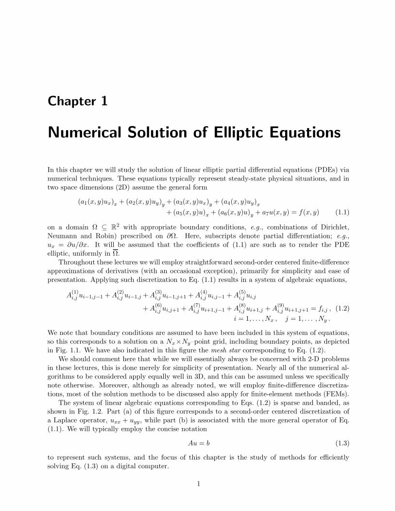
We note that boundary conditions are assumed to have been included in this system of equations,so this corresponds to a solution on a Nx×Ny–point grid, including boundary points, as depictedin Fig. 1.1. We have also indicated in this figure the mesh star corresponding to Eq. (1.2).
We should comment here that while we will essentially always be concerned with 2-D problemsin these lectures, this is done merely for simplicity of presentation. Nearly all of the numerical al-gorithms to be considered apply equally well in 3D, and this can be assumed unless we specificallynote otherwise. Moreover, although as already noted, we will employ finite-difference discretiza-tions, most of the solution methods to be discussed also apply for finite-element methods (FEMs).
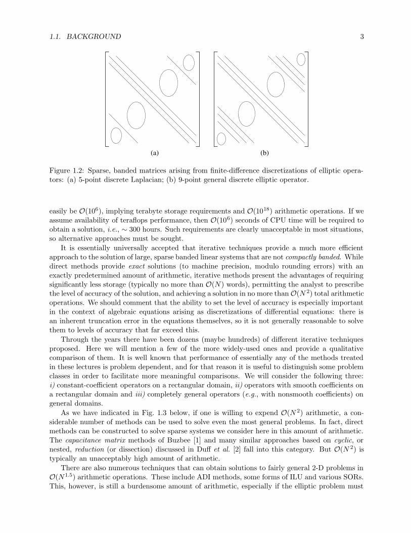
The system of linear algebraic equations corresponding to Eqs. (1.2) is sparse and banded, asshown in Fig. 1.2. Part (a) of this figure corresponds to a second-order centered discretization ofa Laplace operator, uxx + uyy, while part (b) is associated with the more general operator of Eq.(1.1). We will typically employ the concise notation
Au = b (1.3)
to represent such systems, and the focus of this chapter is the study of methods for efficientlysolving Eq. (1.3) on a digital computer.
1

2 CHAPTER 1. NUMERICAL SOLUTION OF ELLIPTIC EQUATIONS
i , j
i =1 i +1i −1 i Nx
j =1
j +1
j
j −1
yN
Figure 1.1: Nx×Ny–point grid and mesh star for discretizations of Eq. (1.1).
In the following sections we will first provide a brief background discussion to motivate study ofthe class of methods to be considered here, namely, iterative techniques, and a short review of thetheory of linear fixed-point iteration. This will be followed by a section devoted to the classical,but still widely-used approach known as successive overrelaxation (SOR). We will then present asummary treatment of a once very popular method known as alternating direction implicit (ADI).In Sec. 1.4 we will consider incomplete LU decomposition (ILU) schemes, and we follow this in Sec.1.5 with a brief discussion of what is termed preconditioning; Sec. 1.6 contains an introduction to theconjugate gradient (CG) method. This will complete our description of older, classical techniques.The two final sections of the chapter will contain introductions to the two modern and extremelypopular approaches for solving sparse linear systems—multigrid (MG) and domain decompositionmethods (DDMs).
1.1 Background
In this section we will first provide an overview of methods available for solving Eq. (1.3) and,in particular, give estimates of the total arithmetic required for each approach. We will concludefrom this that now, and in the immediate future, iterative (as opposed to direct) methods are to bepreferred. We will then present a short theoretical background related to such methods, in general.This will provide a natural introduction to terminology and notation to be used throughout thechapter, and it will give some key theoretical results.
1.1.1 Iterative solution of linear systems—an overview
Linear systems of the form (1.3), with A a nonsingular matrix, can be solved in a great variety ofways. When A is not sparse, direct Gaussian elimination is usually the preferred approach. Butthis requires O(N 2) words of storage and O(N 3) floating-point arithmetic operations for a N×Nmatrix A and N -vectors b and u with N ≡ NxNy. To put this in perspective we note that forsystems arising in the manner of concern in these lectures (viz., as discretizations of PDEs) N can
1.1. BACKGROUND 3
(a) (b)
Figure 1.2: Sparse, banded matrices arising from finite-difference discretizations of elliptic opera-tors: (a) 5-point discrete Laplacian; (b) 9-point general discrete elliptic operator.
easily be O(106), implying terabyte storage requirements and O(1018) arithmetic operations. If weassume availability of teraflops performance, then O(106) seconds of CPU time will be required toobtain a solution, i.e., ∼ 300 hours. Such requirements are clearly unacceptable in most situations,so alternative approaches must be sought.
It is essentially universally accepted that iterative techniques provide a much more efficientapproach to the solution of large, sparse banded linear systems that are not compactly banded. Whiledirect methods provide exact solutions (to machine precision, modulo rounding errors) with anexactly predetermined amount of arithmetic, iterative methods present the advantages of requiringsignificantly less storage (typically no more than O(N) words), permitting the analyst to prescribethe level of accuracy of the solution, and achieving a solution in no more than O(N 2) total arithmeticoperations. We should comment that the ability to set the level of accuracy is especially importantin the context of algebraic equations arising as discretizations of differential equations: there isan inherent truncation error in the equations themselves, so it is not generally reasonable to solvethem to levels of accuracy that far exceed this.
Through the years there have been dozens (maybe hundreds) of different iterative techniquesproposed. Here we will mention a few of the more widely-used ones and provide a qualitativecomparison of them. It is well known that performance of essentially any of the methods treatedin these lectures is problem dependent, and for that reason it is useful to distinguish some problemclasses in order to facilitate more meaningful comparisons. We will consider the following three:i) constant-coefficient operators on a rectangular domain, ii) operators with smooth coefficients ona rectangular domain and iii) completely general operators (e.g., with nonsmooth coefficients) ongeneral domains.
As we have indicated in Fig. 1.3 below, if one is willing to expend O(N 2) arithmetic, a con-siderable number of methods can be used to solve even the most general problems. In fact, directmethods can be constructed to solve sparse systems we consider here in this amount of arithmetic.The capacitance matrix methods of Buzbee [1] and many similar approaches based on cyclic, ornested, reduction (or dissection) discussed in Duff et al. [2] fall into this category. But O(N 2) istypically an unacceptably high amount of arithmetic.
There are also numerous techniques that can obtain solutions to fairly general 2-D problems inO(N1.5) arithmetic operations. These include ADI methods, some forms of ILU and various SORs.This, however, is still a burdensome amount of arithmetic, especially if the elliptic problem must

4 CHAPTER 1. NUMERICAL SOLUTION OF ELLIPTIC EQUATIONS
rectangular domain & smooth coeffs
smooth coeffs
general domains & coefficients
Problem Type
Tot
al A
rithm
etic
N
N log N
N1.25
N1.5
N2 Direct Methods,
Gauss-Seidel, Jacobi
ADI, ILU,optimal SOR
SSOR+CG, ILU+CG
FMG, DDMFMG, DDM
Cyclic ADIfast Poisson solver2-grid MG
Figure 1.3: Qualitative comparison of required arithmetic for various iterative methods.
be solved frequently in the course of solving a more involved overall problem, as often happens incomputational fluid dynamics (CFD) and computational electromagnetics (see, e.g., Fletcher [3],Umashankar and Taflove [4], respectively).
If one restricts attention to problems whose differential operators possess smooth coefficientsthen it is possible to employ combinations of methods to reduce the required arithmetic to O(N 1.25).Examples of this include use of symmetric SOR (SSOR) or ILU as preconditioners for a conjugategradient method, or some form of Krylov-subspace based approach (see Saad [5]). In fact, it ispossible to construct multigrid and domain decomposition techniques that can reduce requiredarithmetic to nearly the optimal O(N) in this case although, as will be evident in the sequel, theseapproaches are quite elaborate.
Finally, for the simple case of a rectangular domain and constant coefficients in the differentialoperators, cyclic ADI, fast Poisson solvers (which are not iterative, but of very limited applica-bility), and two-grid MG methods can produce solutions in O(N log N) total arithmetic, and fullmultigrid (FMG) and DDMs can, of course, lead to solutions in O(N) arithmetic. But we mustcomment that the two conditions, rectangular domain and constant coefficients, are all but mu-tually exclusive in practical problems. Thus, this summary figure, similar to one first presentedby Axelsson [6], indicates that much is involved in selecting a suitable solution method for anyspecific elliptic boundary value problem. But we can expect that an iterative method of some typewill usually be the best choice. In the following sections we will provide details of analyzing andimplementing many of the abovementioned techniques.
1.1. BACKGROUND 5
1.1.2 Basic theory of linear iterative methods
In this section we will present a brief overview of fixed-point iteration as applied to the solutionof linear systems. This will provide an opportunity to introduce terminology and notation to beused throughout the lectures of Chap. 1, and in addition to introduce some theoretical tools thatare not only useful for analysis but also adaptable to numerical calculation. We begin by recallingEq. (1.3),
Au = b ,
and note that iterative methods for solving this system of linear equations can essentially alwaysbe expressed in the form
u(n+1) = Gu(n) + k . (1.4)
In this expression (n) denotes an iteration counter, and G is the iteration matrix; it is related tothe system matrix A by
G = I − Q−1A , (1.5)
where I is the identity matrix, and Q is generally called the splitting matrix.It is worthwhile to consider a well-known concrete example to motivate this terminology. Recall
from elementary numerical analysis (see, e.g., Stoer and Bulirsch [7]) that Jacobi iteration can beconstructed as follows. First, decompose the matrix A as
A = D − L − U , (1.6)
where D is the diagonal of A, and L and U are negatives of the lower and upper, respectively,triangles of A. Now substitute (1.6) into (1.3) to obtain
(D − L − U)u = b ,
or
Du = (L + U)u + b . (1.7)
In deriving Eq. (1.7) we have “split” the matrix A to isolate the trivially invertible diagonalmatrix on the left-hand side. We now introduce iteration counters and write (1.7) as
u(n+1) = D−1(L + U)u(n) + D−1b . (1.8)
Now observe from (1.6) that
L + U = D − A ,
soD−1(L + U) = I − D−1A .
Thus, D is the splitting matrix, and Eq. (1.8) is in the form (1.4) with
G ≡ D−1(L + U) = I − D−1A , and k ≡ D−1b . (1.9)
We see from this that the splitting matrix can be readily identified as the inverse of the matrixmultiplying the original right-hand side vector of the system in the definition of k.
We should next recall that convergence of fixed-point iterations generally requires somethingof the nature of guaranteeing existence of a Lipschitz condition with Lipschitz constant less thanunity. The following theorem provides the version of this basic notion that is of use for the studyof linear iterative methods.
6 CHAPTER 1. NUMERICAL SOLUTION OF ELLIPTIC EQUATIONS
Theorem 1.1 A necessary and sufficient condition for convergence of the iterations (1.4) to thesolution of Eq. (1.3) from any initial guess is
ρ(G) < 1 , (1.10)
whereρ(G) ≡ max
1≤i≤N|λi| , λi ∈ σ(G) , (1.11)
is the spectral radius of the iteration matrix G, and σ(G) is notation for the spectrum (set of alleigenvalues) of G.
We remark (without proof) that this basically follows from the contraction mapping principleand the fact that
ρ(G) ≤ ‖G‖ (1.12)
for all norms, ‖ · ‖. We also note that convergence may occur even when ρ(G) ≤ 1 holds, but onlyfor a restricted set of initial guesses. It should be clear that ρ(G) corresponds to the Lipschitzconstant mentioned above.
We next present some definitions that will be of use throughout these lectures. We first considerseveral definitions of error associated with the iterations (1.4), and then we define convergence rateto quantify how rapidly error is reduced.
Definition 1.1 The residual after n iterations is
rn = b − Au(n) . (1.13)
Definition 1.2 The exact error after n iterations is
en = u − u(n) . (1.14)
Definition 1.3 The iteration error after n iterations is
dn = u(n+1) − u(n) . (1.15)
We note that it is easy to show that rn and en are related by
Aen = rn . (1.16)
Also, it follows from the general linear iteration formula (1.4) and the definition (1.14) that
en = Gen−1 = G2en−2 = · · · = Gne0 , (1.17)
and similarly for dn. This leads to the following.
Definition 1.4 The average convergence rate (over n iterations) for iterations of Eq. (1.4) is givenby
Rn(G) ≡ − 1
nlog ‖Gn‖ . (1.18)
This definition is motivated by the fact that from (1.17)
log ‖en‖ − log ‖e0‖ ≤ log ‖Gn‖
for compatible matrix and vector norms, and thus Rn(G) is a measure of the average (logarithmic)error reduction over n iterations.
A second important definition associated with convergence rate is the following.
1.1. BACKGROUND 7
Definition 1.5 The asymptotic convergence rate for the iterations (1.4) is defined as
R∞(G) ≡ − log ρ(G) . (1.19)
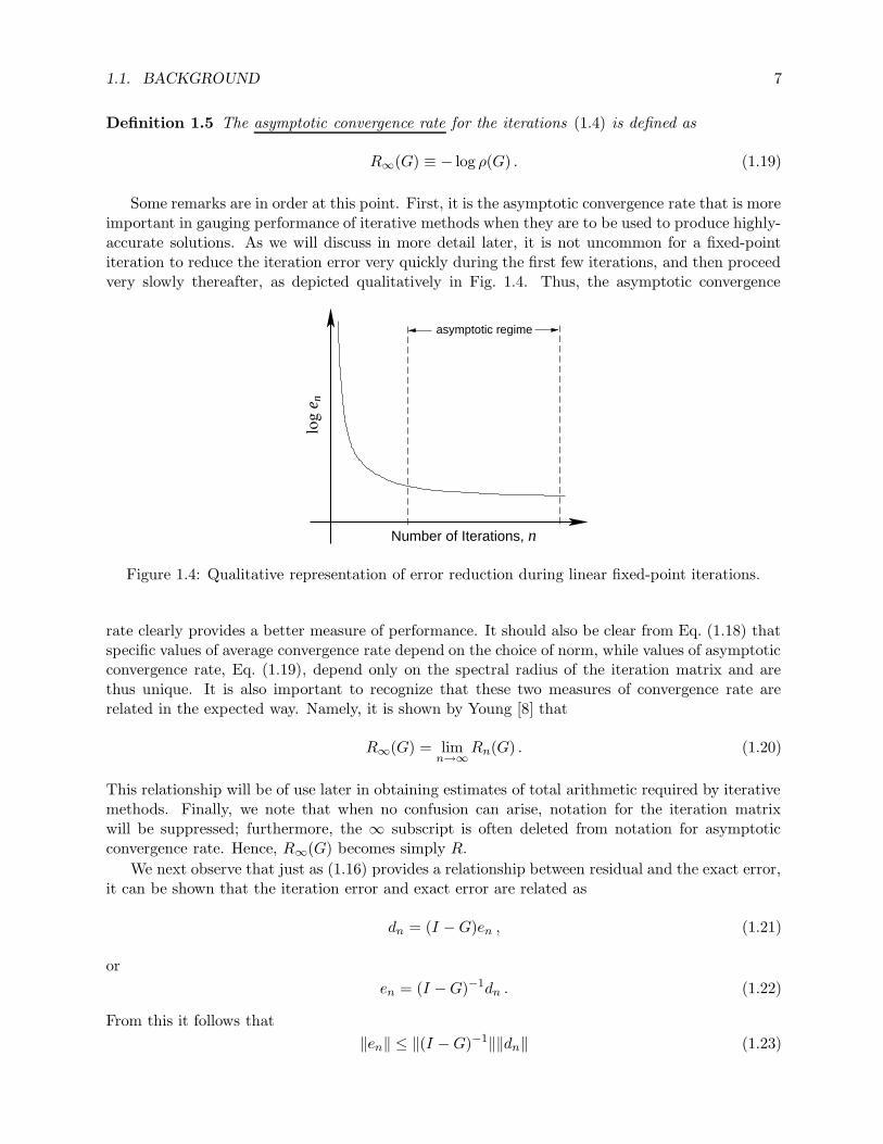
Some remarks are in order at this point. First, it is the asymptotic convergence rate that is moreimportant in gauging performance of iterative methods when they are to be used to produce highly-accurate solutions. As we will discuss in more detail later, it is not uncommon for a fixed-pointiteration to reduce the iteration error very quickly during the first few iterations, and then proceedvery slowly thereafter, as depicted qualitatively in Fig. 1.4. Thus, the asymptotic convergence
Number of Iterations, n
log
e nasymptotic regime
Figure 1.4: Qualitative representation of error reduction during linear fixed-point iterations.
rate clearly provides a better measure of performance. It should also be clear from Eq. (1.18) thatspecific values of average convergence rate depend on the choice of norm, while values of asymptoticconvergence rate, Eq. (1.19), depend only on the spectral radius of the iteration matrix and arethus unique. It is also important to recognize that these two measures of convergence rate arerelated in the expected way. Namely, it is shown by Young [8] that
R∞(G) = limn→∞
Rn(G) . (1.20)
This relationship will be of use later in obtaining estimates of total arithmetic required by iterativemethods. Finally, we note that when no confusion can arise, notation for the iteration matrixwill be suppressed; furthermore, the ∞ subscript is often deleted from notation for asymptoticconvergence rate. Hence, R∞(G) becomes simply R.
We next observe that just as (1.16) provides a relationship between residual and the exact error,it can be shown that the iteration error and exact error are related as
dn = (I − G)en , (1.21)
or
en = (I − G)−1dn . (1.22)
From this it follows that
‖en‖ ≤ ‖(I − G)−1‖‖dn‖ (1.23)
8 CHAPTER 1. NUMERICAL SOLUTION OF ELLIPTIC EQUATIONS
for compatible matrix and vector norms. Moreover, if we take the matrix norm to be the spectralnorm and the vector norm the 2-norm, then if G is diagonalizable it follows that
‖en‖ ≤ 1
1 − ρ(G)‖dn‖ (1.24)
for ρ(G) < 1.The importance of this result should be clear. The exact error is what we would like to know,
but to actually compute it requires as much work as computing the exact solution, as is clear from(1.16). On the other hand, dn is easily computed. At the same time, ρ(G) can often be estimatedquite accurately (and inexpensively), either theoretically or numerically, as we will see below. It isalso important to observe that Eq. (1.24) implies that ‖en‖ can be very much greater than ‖dn‖. Inparticular, as ρ(G) → 1, the coefficient of ‖dn‖ on the right-hand side of (1.24) grows unboundedly.Thus, the inexpensively computed ‖dn‖ may not provide a good measure of solution accuracy. Thismakes estimation of ρ(G) quite important. The following theorem provides a very effective mannerin which this can be done.
Theorem 1.2 Let en and dn be as defined in Eqs. (1.14) and (1.15), respectively, and supposeρ(G) < 1 holds. Then for any norm, ‖ · ‖,
limn→∞
‖dn‖‖dn−1‖
= ρ(G) , (1.25)
and
limn→∞
‖en‖‖dn‖
=1
1 − ρ(G). (1.26)
Proof. We will prove these only for the 2-norm. For a complete proof the reader is referred to [8].To prove the first of these we again recall that
dn = Gdn−1 ,
which implies‖dn‖ ≤ ‖G‖‖dn−1‖
for compatible norms. In particular, if we take the vector norm to be the 2-norm we may use thespectral norm as the matrix norm. Then if G is diagonalizable we have
‖G‖ = ρ(G) .
Thus,‖dn‖‖dn−1‖
≤ ρ(G) .
Next, we employ the Rayleigh quotient to arrive at the reverse inequality. Namely, we havesince dn is an eigenvector of G for n → ∞ (this is clear from a formula for dn analogous to (1.17),and the form of the power method for finding eigenvalues),
ρ(G) =〈dn−1, Gdn−1〉
‖dn−1‖2=
〈dn−1, dn〉‖dn−1‖2
.
But by the Cauchy-Schwarz inequality it follows that
ρ(G) ≤ ‖dn−1‖‖dn‖‖dn−1‖2
=‖dn‖‖dn−1‖
,

1.2. SUCCESSIVE OVERRELAXATION 9
thus completing the proof of (1.25) for the case of the 2-norm.To prove (1.26) we first note that we have already shown in (1.24) that
‖en‖‖dn‖
≤ 1
1 − ρ(G).
Now from (1.21) we also have(I − G)en = dn ,
and‖(I − G)en‖ = ‖dn‖ .
This implies‖dn‖ ≤ ‖(I − G)‖‖en‖ ,
again, for compatible matrix and vector norms. So using the matrix spectral norm and the vector2-norm, respectively, gives
‖en‖‖dn‖
≥ 1
1 − ρ(G),
completing the proof.This concludes our introduction to basic linear fixed-point iteration.
1.2 Successive Overrelaxation
In this section we will provide a fairly complete description of one of the historically most-usediterative methods for solution of sparse linear systems, viz., successive overrelaxation (SOR). As iswell known, SOR can be developed as the last step in a sequence of methods beginning with Jacobiiteration, proceeding through Gauss-Seidel iteration, and arriving, finally, at SOR. It is also the casethat much of the rigorous theory of SOR (see Young [8]) relies on the theory of Jacobi iteration.Thus, we will begin our treatment of SOR with some basic elements of Jacobi iteration theory.We will then continue with the theory of SOR, itself, culminating in the main theorem regardingoptimal SOR iteration parameters. We then consider several modifications to basic “point” SORthat are widely used in implementations, devoting a section to each of red-black ordered SOR,symmetric SOR (SSOR) and finally successive line overrelaxation (SLOR).
1.2.1 Jacobi iteration
Throughout most of our discussions we will usually be concerned with the basic mathematical prob-lem of Laplace’s (or Poisson’s) equation with Dirichlet boundary conditions on a 2-D rectangulardomain Ω; that is,
uxx + uyy = f(x, y) , (x, y) ∈ Ω ⊆ R2 , (1.27a)
withu(x, y) = g(x, y) , (x, y) ∈ ∂Ω . (1.27b)
Here, Ω ≡ [ax, bx]× [ay, by], and f and g are given functions assumed to be in C(Ω), or C(∂Ω),respectively.

10 CHAPTER 1. NUMERICAL SOLUTION OF ELLIPTIC EQUATIONS
We will employ a standard second-order centered discretization,
ui−1,j − 2ui,j + ui+1,j
h2x
+ui,j−1 − 2ui,j + ui,j+1
h2y
= fi,j , i, j = 2, 3, . . . , Nx−1(Ny−1) , (1.28a)
with
ui,j = gi,j , i = 1 or Nx with j = 1, . . . , Ny (1.28b)
j = 1 or Ny with i = 1, . . . , Nx .
We will assume uniform grid spacing in each of the separate directions. This problem setup isshown in Fig. 1.5, a modification of Fig. 1.1 for the special case of the Laplacian considered here.We calculate hx and hy from
ax
ya
bx
i = Nx
by
j = Ny
i
j
Figure 1.5: Discretization of the Laplace/Poisson equation on a rectangular grid of Nx×Ny points.
hx =bx − ax
Nx − 1, hy =
by − ay
Ny − 1,
respectively. But we will typically set hx = hy = h for most analyses, and in this case Eqs. (1.28)collapse to
ui−1,j + ui,j−1 − 4ui,j + ui,j+1 + ui+1,j = h2fi,j , i, j = 2, 3, . . . , Nx(Ny) (1.29)
with boundary conditions as before. If we now “solve” (1.29) for ui,j, we obtain the Jacobi iterationformula
u(n+1)i,j =
1
4
[u
(n)i−1,j + u
(n)i,j−1 + u
(n)i,j+1 + u
(n)i+1,j − h2fi,j
](1.30)
∀ i, j in the index set of Eq. (1.29). This set of equations is clearly in fixed-point form and thuscan be expressed as
u(n+1) = Bu(n) + k , (1.31)
1.2. SUCCESSIVE OVERRELAXATION 11
. . .
0
0
0
0
0
0
0
0
. . .
. . .. . .
. . .. . .
. . .
Figure 1.6: Band structure of Jacobi iteration matrix for Laplace/Poisson equation.
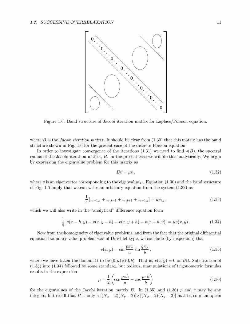
where B is the Jacobi iteration matrix. It should be clear from (1.30) that this matrix has the bandstructure shown in Fig. 1.6 for the present case of the discrete Poisson equation.
In order to investigate convergence of the iterations (1.31) we need to find ρ(B), the spectralradius of the Jacobi iteration matrix, B. In the present case we will do this analytically. We beginby expressing the eigenvalue problem for this matrix as
Bv = µv , (1.32)
where v is an eigenvector corresponding to the eigenvalue µ. Equation (1.30) and the band structureof Fig. 1.6 imply that we can write an arbitrary equation from the system (1.32) as
1
4[vi−1,j + vi,j−1 + vi,j+1 + vi+1,j] = µvi,j , (1.33)
which we will also write in the “analytical” difference equation form
1
4[v(x − h, y) + v(x, y − h) + v(x, y + h) + v(x + h, y)] = µv(x, y) . (1.34)
Now from the homogeneity of eigenvalue problems, and from the fact that the original differentialequation boundary value problem was of Dirichlet type, we conclude (by inspection) that
v(x, y) = sinpπx
asin
qπy
b, (1.35)
where we have taken the domain Ω to be (0, a)×(0, b). That is, v(x, y) = 0 on ∂Ω. Substitution of(1.35) into (1.34) followed by some standard, but tedious, manipulations of trigonometric formulasresults in the expression
µ =1
2
(cos
pπh
a+ cos
pπh
b
)(1.36)
for the eigenvalues of the Jacobi iteration matrix B. In (1.35) and (1.36) p and q may be anyintegers; but recall that B is only a [(Nx − 2)(Ny − 2)]×[(Nx − 2)(Ny − 2)] matrix, so p and q can

12 CHAPTER 1. NUMERICAL SOLUTION OF ELLIPTIC EQUATIONS
take on values only between 1 and Nx − 2 and 1 and Ny − 2, respectively, before repetitions beginto occur in the values of µ calculated from (1.36).
Our task now is to find ρ(B), i.e., to find the maximum value of µ for p and q in the aboveranges. It is easy to check by inspection that this maximum occurs for p = q = 1, yielding theresult
ρ(B) =1
2
(cos
πh
a+ cos
πh
b
). (1.37)
This is the exact spectral radius of the Jacobi iteration matrix for a second-order centered-differenceapproximation to a Dirichlet problem for Laplace’s (Poisson’s) equation on a Nx×Ny gridding ofthe rectangular domain Ω = (0, a)×(0, b). Clearly, it follows that the corresponding result for Ωthe unit square is
ρ(B) = cos πh . (1.38)
To obtain further analytical results it is convenient to expand (1.37) in a Taylor series as
ρ(B) = 1 − 1
4
[(π
a
)2+(π
b
)2]
h2 + O(h4) , (1.39)
from which it follows (after yet another Taylor expansion) that the asymptotic convergence ratefor Jacobi iterations is
R∞(B) = − log ρ(B) =1
4
[(π
a
)2+(π
b
)2]
h2 + O(h4) . (1.40)
Again, for the special case of the unit square, this is
R∞(B) =1
2π2h2 + O(h4) . (1.41)
It is important to recognize that R∞(B) ∼ h2, so as the grid spacing of a discrete method isdecreased to obtain better accuracy the convergence rate decreases as the square of h. This ulti-mately leads to large expenditures of floating-point arithmetic in applications of Jacobi’s method,as we will now demonstrate in a more quantitative way.
We can use the preceding analysis to estimate the total arithmetic required by a Jacobi iterationprocedure to reduce the error in a computed solution by a factor r. To begin we recall that theaverage convergence rate given in Eq. (1.18) provides a formula for the number of iterations, n:
n = − 1
Rnlog ‖Gn‖ .
Also, from (1.17) we have‖en‖‖e0‖
≤ ‖Gn‖ .
Now note that ‖en‖/‖e0‖ is an error reduction ratio that might be prescribed by a user of an ellipticequation solving program; we denote this by r:
r ≡ ‖en‖‖e0‖
.
Then
n = − 1
Rnlog r ,

1.2. SUCCESSIVE OVERRELAXATION 13
with log r ∼ O(1) to O(10) being typical.
At this point we recall that Rn → R∞ as n → ∞, and assume n is sufficiently large thatRn ' R∞. It then follows that the required number of Jacobi iterations to reduce the error by afactor r below the initial error is
n ≤ − 112π2h2
log r , (1.42)
and since h ∼ 1/Nx this implies that n ∼ O(N). Finally, at each iteration O(N) arithmeticoperations will be required, so the total arithmetic for Jacobi iteration is O(N 2).
1.2.2 SOR theory
We recall from elementary numerical analysis that SOR is obtained as an extrapolated version ofGauss-Seidel iteration (which, itself, is derived from the preceding Jacobi iterations), and neitherGauss-Seidel nor SOR appear as fixed-point iterations in their computational forms. We havealready seen the value of the analysis that is available for fixed-point iterations, so it is naturalto convert SOR to this form in order to attempt prediction of its optimal iteration parameterand its required total arithmetic. We begin this section by deriving this fixed-point form. Thenwe introduce a series of definitions and theorems associated with convergence of Jacobi and SORiterations, culminating in a theorem containing an explicit formula for the optimal SOR iterationparameter, ωb, expressed in terms of the spectral radius of the Jacobi iteration matrix.
Fixed-point form of SOR
We again consider the linear system
Au = b , (1.43)
where A is a sparse, nonsingular N×N matrix, and decompose A as
A = D − L − U , (1.44)
as was done earlier in Eq. (1.6). Substitution of this into (1.43) followed by some rearrangementleads to
(D − L)u(n+1) = Uu(n) + b , (1.45)
or
D(I − D−1L)u(n+1) = Uu(n) + b ,
and
u(n+1) = (I − D−1L)−1D−1Uu(n) + (I − D−1L)−1D−1b . (1.46)
This is the fixed-point form of Gauss-Seidel iteration, and it is clearly in the usual linear fixed-pointform
u(n+1) = Gu(n) + k .
In the present case we define
L ≡ (I − D−1L)−1D−1U , (1.47a)
k ≡ (I − D−1L)−1D−1b , (1.47b)
and write
u(n+1) = Lu(n) + k . (1.48)

14 CHAPTER 1. NUMERICAL SOLUTION OF ELLIPTIC EQUATIONS
We now recall that successive overrelaxation is obtained from Gauss-Seidel iteration by intro-ducing the relaxation parameter ω via the extrapolation
u(n+1) = (1 − ω)u(n) + ωu(n+1)∗ , (1.49)
where u(n+1)∗ has been obtained from (1.48). This leads us to the fixed-point formula for SORiterations:
u(n+1) = (1 − ω)u(n) + ω[D−1Lu(n+1) + D−1Uu(n) + D−1b
],
oru(n+1) = (I − ωD−1L)−1
[ωD−1U + (1 − ω)I
]u(n) + ω(I − ωD−1L)−1D−1b . (1.50)
We note that the equation preceding (1.50) is easily obtained from the “computational” form ofGauss-Seidel iterations,
u(n+1)∗ = D−1Lu(n+1) + D−1Uu(n) + D−1b , (1.51)
a rearrangement of Eq. (1.45). If we now define
Lω ≡ (I − ωD−1L)−1[ωD−1U + (1 − ω)I
], (1.52a)
kω ≡ ω(I − ωD−1L)−1D−1b , (1.52b)
we can write Eq. (1.50) asu(n+1) = Lωu(n) + kω , (1.53)
the fixed-point form of SOR. It is important to note that although this form is crucial for analysisof SOR, it is not efficient for numerical calculations. For this purpose the combination of (1.51)and (1.49) should always be used.
Consistent ordering and property A
We now introduce some important definitions and theorems leading to the principal theoremin SOR theory containing formulas for the optimal SOR parameter and the spectral radius of Lω.There are two crucial notions that ultimately serve as necessary hypotheses in the majority oftheorems associated with SOR: consistently ordered and property A. To motivate the need for thefirst of these we recall that in contrast to Jacobi iterations, in SOR the order in which individualequations of the system are evaluated influences the convergence rate, and even whether convergenceoccurs. This is easily recognized by recalling the computational formulas for SOR, written here fora second-order centered finite-difference approximation of the Poisson equation:
u(n+1)∗
i,j =1
4
[u
(n+1)i−1,j + u
(n+1)i,j−1 + u
(n)i,j+1 + u
(n)i+1,j − h2fi,j
], (1.54a)
u(n+1)i,j = ωu
(n+1)∗
i,j + (1 − ω)u(n)i,j , (1.54b)
for grid point (i, j). Obviously, reordering the sequence of evaluation of the ui,js will change whichof the values are known at the advanced iteration level on the right-hand side of Eq. (1.54a). Inturn, this will have an effect on the matrix representation of the fixed-point form of this procedure,and thus also on the spectral radius. In particular, there are problems for which it is possiblefor some orderings to be convergent and others divergent. In order to make precise statementsregarding convergence of SOR we will need the notion of a consistently-ordered matrix given in thefollowing definition.Definition 1.6 The N×N matrix A is consistently ordered if for some K ∃ disjoint subsets S1, S2,
. . . , SK ⊂ W = 1, 2, . . . , N 3 ∪Kk=1Sk = W , and for i ∈ Sk with either ai,j 6= 0 or aj,i 6= 0, then
j ∈ Sk+1 for j > i, and j ∈ Sk−1 for j < i.
1.2. SUCCESSIVE OVERRELAXATION 15
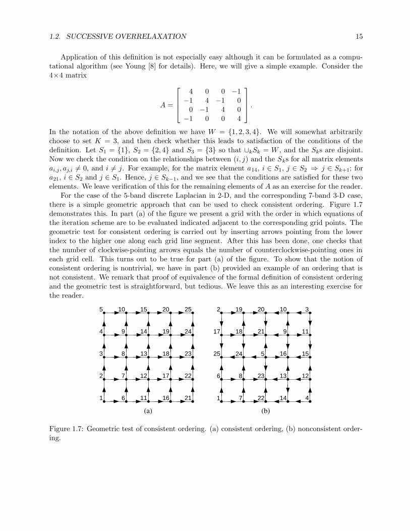
Application of this definition is not especially easy although it can be formulated as a compu-tational algorithm (see Young [8] for details). Here, we will give a simple example. Consider the4×4 matrix
A =
4 0 0 −1−1 4 −1 0
0 −1 4 0−1 0 0 4
.
In the notation of the above definition we have W = 1, 2, 3, 4. We will somewhat arbitrarilychoose to set K = 3, and then check whether this leads to satisfaction of the conditions of thedefinition. Let S1 = 1, S2 = 2, 4 and S3 = 3 so that ∪kSk = W , and the Sks are disjoint.Now we check the condition on the relationships between (i, j) and the Sks for all matrix elementsai,j, aj,i 6= 0, and i 6= j. For example, for the matrix element a14, i ∈ S1, j ∈ S2 ⇒ j ∈ Sk+1; fora21, i ∈ S2 and j ∈ S1. Hence, j ∈ Sk−1, and we see that the conditions are satisfied for these twoelements. We leave verification of this for the remaining elements of A as an exercise for the reader.
For the case of the 5-band discrete Laplacian in 2-D, and the corresponding 7-band 3-D case,there is a simple geometric approach that can be used to check consistent ordering. Figure 1.7demonstrates this. In part (a) of the figure we present a grid with the order in which equations ofthe iteration scheme are to be evaluated indicated adjacent to the corresponding grid points. Thegeometric test for consistent ordering is carried out by inserting arrows pointing from the lowerindex to the higher one along each grid line segment. After this has been done, one checks thatthe number of clockwise-pointing arrows equals the number of counterclockwise-pointing ones ineach grid cell. This turns out to be true for part (a) of the figure. To show that the notion ofconsistent ordering is nontrivial, we have in part (b) provided an example of an ordering that isnot consistent. We remark that proof of equivalence of the formal definition of consistent orderingand the geometric test is straightforward, but tedious. We leave this as an interesting exercise forthe reader.
1
2
3
4
5
6
7
8
9
10
11
12
13
14
15
16
17
18
19
20
21
22
23
24
25
1
2 3
4
5
6
7
8
9
10
11
1213
14
1516
17 18
19 20
21
22
23
2425
(a) (b)
Figure 1.7: Geometric test of consistent ordering. (a) consistent ordering, (b) nonconsistent order-ing.
16 CHAPTER 1. NUMERICAL SOLUTION OF ELLIPTIC EQUATIONS
We also remark that the ordering in part (a) of the figure is one of two natural orderings, theother one corresponding to increasing the index first in the horizontal direction. Both orderingsare widely used in practice.
The consistent-ordering property has numerous characterizations. Here, we present an addi-tional one that is widely quoted, and sometimes used as the definition of consistently ordered.
Theorem 1.3 If the matrix A is consistently ordered, then det(αL + 1αU − κD) is independent of
α (α 6= 0) ∀ κ.
Our first result to make use of the consistent-ordering property is contained in the following.
Theorem 1.4 Let A be a symmetric, consistently-ordered matrix with positive diagonal elements.Then ρ(B) < 1 iff A is positive definite.
This theorem provides a very strong result concerning convergence of Jacobi iterations.The definition of consistently ordered given above is clearly quite tedious to apply, as is high-
lighted by the simple example. We have seen that in some cases it is possible to employ a fairlyeasy geometric test, but this cannot be applied to the general 9-point discrete operator consideredin Eq. (1.2) and Fig. 1.1. This motivates the search for at least a nearly equivalent property thatis easier to test, leading us to consider the characterization known as property A.
Definition 1.7 A N×N matrix A has property A if ∃ two disjoint subsets S1, S2⊂W ≡1, 2, . . . , N3 S1∪S2 = W , and if i 6=j and either ai,j 6=0 or aj,i 6=0, then i ∈ S1 ⇒ j ∈ S2, or i ∈ S2 ⇒ j ∈ S1.
The importance of property A is that it slightly widens the class of matrices to which SOR theorymay be applied, and at the same time it provides a more readily checkable characterization of thesematrices. In particular, not every matrix having property A is consistently ordered. However, wehave the following theorem, which we state without proof (see [8] for a proof) that connects thesetwo matrix properties.
Theorem 1.5 Let the matrix A have property A. Then ∃ a permutation matrix P 3 A ′ = P−1APis consistently ordered.
It is clear that the matrix P generates a similarity transformation, and hence A ′ which isconsistently ordered has the same spectrum as A, which has only property A. Thus, any spectralproperties (the spectral radius, in particular) that hold for a consistently-ordered matrix also holdfor a matrix having property A. But the similarity transformation of the theorem does not lead toconsistent ordering for all permutation matrices P , so analyses involving these ideas must includefinding an appropriate matrix P .
Optimal SOR parameter
In this subsection we will present a formula for the optimal SOR relaxation parameter, denotedωb. Our treatment will rely on the preceding results, and follows that found in [8]. But we notethat similar results can be obtained from basically geometric arguments, as also given in [8] andelsewhere, e.g., Mitchell and Griffiths [9] and Varga [10]. We begin by stating a pair of theorems thatare needed in the proof of the main theorem concerning the value of the optimal SOR parameter.
For consistently-ordered matrices it can be shown (see e.g., [9]) that the eigenvalues of the SORiteration matrix are related to those of the Jacobi iteration matrix (which can often be calculatedexactly) by the formula given in the following theorem.
1.2. SUCCESSIVE OVERRELAXATION 17
Theorem 1.6 Suppose the matrix A is consistently ordered, and let B and Lω be the Jacobi andSOR, respectively, iteration matrices associated with A. Let µ ∈ σ(B) and λ ∈ σ(Lω), ω being theSOR iteration parameter. Then
λ − ωµλ1/2 + ω − 1 = 0 . (1.55)
Our first result regarding the SOR parameter ω is the following.
Theorem 1.7 Suppose A is consistently ordered with nonvanishing diagonal elements, and suchthat the Jacobi iteration matrix B has real eigenvalues. Then ρ(Lω) < 1 iff 0 < ω < 2, andρ(B) < 1.
Proof. The proof follows directly from the following lemma applied to (1.55).
Lemma If b, c ∈ R, then both roots of
x2 − bx + c = 0
have modulus less than unity iff |b| < 1 + c and |c| < 1.Proof of the lemma follows from a direct calculation, which we omit. (It can be found in [8],
pg. 172.)
Now take b = ωµ, and c = ω − 1, viewing (1.55) as a quadratic in λ1/2. Since µ ∈ σ(B), proofof the theorem is immediate.
We now state without proof the main result regarding the optimal SOR parameter, ωb.
Theorem 1.8 (Optimal SOR parameter) Suppose A is a consistently-ordered matrix, and theJacobi iteration matrix has σ(B)∈R with µ ≡ ρ(B) < 1. Then the optimal SOR iteration parameteris given by
ωb =2
1 + (1 − µ2)1/2. (1.56)
Moreover, ∀ ω ∈ (0, 2)
ρ(Lω) =
[ωµ+(ω2µ2−4(ω−1))1/2
2
]20 < ω < ωb
ω − 1 ωb < ω < 2 .(1.57)
Furthermore, ρ(Lω) is a strictly decreasing function of ω for ω ∈ (0, ωb), and ρ(Lω) > ρ(Lωb) for
ω 6= ωb .
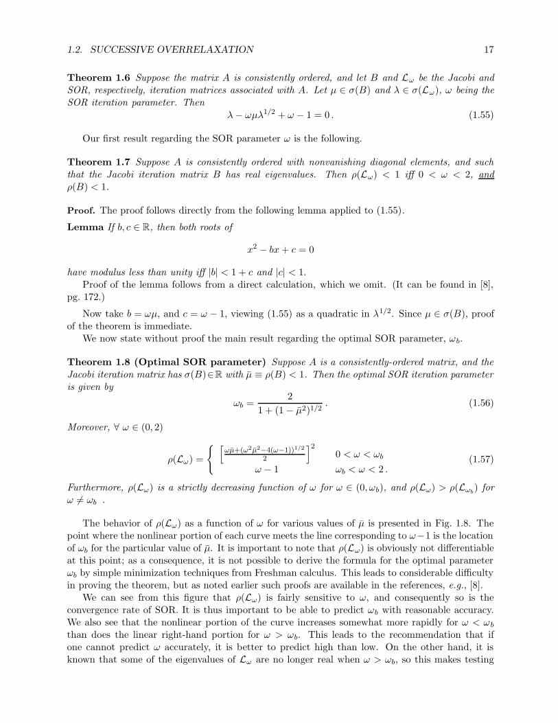
The behavior of ρ(Lω) as a function of ω for various values of µ is presented in Fig. 1.8. Thepoint where the nonlinear portion of each curve meets the line corresponding to ω−1 is the locationof ωb for the particular value of µ. It is important to note that ρ(Lω) is obviously not differentiableat this point; as a consequence, it is not possible to derive the formula for the optimal parameterωb by simple minimization techniques from Freshman calculus. This leads to considerable difficultyin proving the theorem, but as noted earlier such proofs are available in the references, e.g., [8].
We can see from this figure that ρ(Lω) is fairly sensitive to ω, and consequently so is theconvergence rate of SOR. It is thus important to be able to predict ωb with reasonable accuracy.We also see that the nonlinear portion of the curve increases somewhat more rapidly for ω < ωb
than does the linear right-hand portion for ω > ωb. This leads to the recommendation that ifone cannot predict ω accurately, it is better to predict high than low. On the other hand, it isknown that some of the eigenvalues of Lω are no longer real when ω > ωb, so this makes testing

18 CHAPTER 1. NUMERICAL SOLUTION OF ELLIPTIC EQUATIONS
0.0 0.5 1.0 1.5 2.00.4
0.6
0.8
1.0
ω
µ = 0.9
ρ(L
) ω µ = 0.95
µ = 0.99
µ = 0.999
ω −1
Figure 1.8: Spectral radius of SOR iteration matrix vs. ω.
convergence of a solution more difficult due to oscillations in the iteration error induced by thecomplex eigenvalues. Finally, we observe from the figure that ωb increases monotonically with µ(= ρ(B)), which itself increases monotonically with decreasing grid spacing h, as is clear from Eqs.(1.37) and (1.39).
SOR convergence rate
In this subsection we will provide an estimate of the convergence rate for optimal SOR and usethis to predict total floating-point arithmetic requirements, just as we were able to do earlier forJacobi iterations. The key result needed for this is the following theorem which is proved in [8].Theorem 1.9 Let A be a consistently-ordered matrix with nonvanishing diagonal elements 3 σ(B) ∈R and 3 µ ≡ ρ(B) < 1. Then
2µ[R(L)]1/2 ≤ R(Lωb) ≤ R(L) + 2[R(L)]1/2 ,
with the right-hand inequality holding when R(L) ≤ 3. Furthermore,
limµ→1−
[R(Lωb)/2(R(L))1/2] = 1 . (1.58)
We will use this result to calculate the asymptotic convergence rate for optimal SOR for aLaplace-Dirichlet problem posed on the unit square. Recall from Eq. (1.38) that the spectral radiusof the Jacobi iteration matrix is cos πh for this case, with h being the uniform finite-difference gridspacing. Furthermore, Eq. (1.41) gives R(B) = 1
2π2h2 + O(h4). Now it is easy to show thatGauss-Seidel iterations converge exactly twice as fast as do Jacobi iterations for this case; i.e.,R(L) = 2R(B). To see this recall Eq. (1.55) in Theorem 1.6, and set ω = 1 in that formula. Itfollows that λ = µ2, and from this we would intuitively expect that
ρ(L) = µ2 ,
from which the result follows. We note however, that there are some missing technical details thatwe will mention, but not attempt to prove. In particular, although the correspondence λ = µ2
1.2. SUCCESSIVE OVERRELAXATION 19
follows easily, providing a relationship between eigenvalues of the Gauss-Seidel and Jacobi iterationmatrices, this alone does not imply that their spectral radii are similarly related—in a sense, this isa “counting” (or ordering) problem: the eigenvalue that corresponds to the spectral radius of B isnot necessarily related by the above formula to the eigenvalue corresponding to the spectral radiusof L. We comment that this is one of the questions that must be dealt with in proving the mainSOR theorem. Hence, the desired result may be presumed to be true.
Now from (1.58), as h → 0 (µ → 1−) we have
R(Lωb) → 2[R(L)]1/2 ' 2πh . (1.59)
It is of interest to consider the practical consequences of this result. Using the above togetherwith R(L) = 2R(B) = π2h2 yields
R(Lωb)
R(L)' 2
πh,
which implies that for even relatively coarse gridding, say h = 1/20, this ratio is greater than 12.This indicates that the convergence rate of optimal SOR is more than an order of magnitude greaterthan that of Gauss-Seidel, even on a coarse grid. The above formula clearly shows that as h → 0the ratio of improvement obtained from using optimal ω becomes very large.
Related to this is the fact (from Eq. (1.59)) that R(Lωb) ∼ O(h); that is, the convergence rate
decreases only linear with Nx (or Ny) when ω = ωb, in contrast to a rate of decrease proportionalto N (= NxNy) found for Jacobi and Gauss-Seidel iterations. This immediately implies that therequired total arithmetic on a Nx×Ny finite-difference grid is O(N 1.5) for SOR with the optimalrelaxation parameter. We leave as an exercise for the reader demonstration that in 3D the totalarithmetic for optimal SOR is O(N 1.33...).
1.2.3 Some modifications to basic SOR
In this section we will briefly describe some modifications that can be made to the basic SORprocedure considered to this point. There are many such modifications, and various of these aretreated in detail in, e.g., Hageman and Young [11] and elsewhere. Here we will study only thefollowing three: i) red-black ordering, ii) symmetric SOR and iii) line SOR. Each of these providesspecific advantages not found in basic point SOR; but, in general, it is not always clear thatthese advantages are sufficient to offset the attendant increased algorithmic complexities of theseapproaches.
Red-black ordering
Red-black ordering, so named because of the “checkerboard” patterning of indexing of the un-knowns, offers the advantage that the resultant coeeficient matrix is (for the discrete Laplacian)automatically consistently ordered. Numerical experiments indicate somewhat higher convergencerates than are achieved with natural orderings, although this seems to be problem dependent.
For a solution vector
u = (u1,1, u1,2, . . . , u1,Ny , u2,1, . . . , . . . , uNx,Ny)T ,
which is ordered in one of the two natural orderings, the red-black ordering is obtained as follows.We decompose this solution vector into two subvectors, a “red” one and a “black” one defined suchthat the sums of their (i, j) indices are, respectively even and odd. That is, for the red vector i + jis even, and for the black vector it is odd.
20 CHAPTER 1. NUMERICAL SOLUTION OF ELLIPTIC EQUATIONS
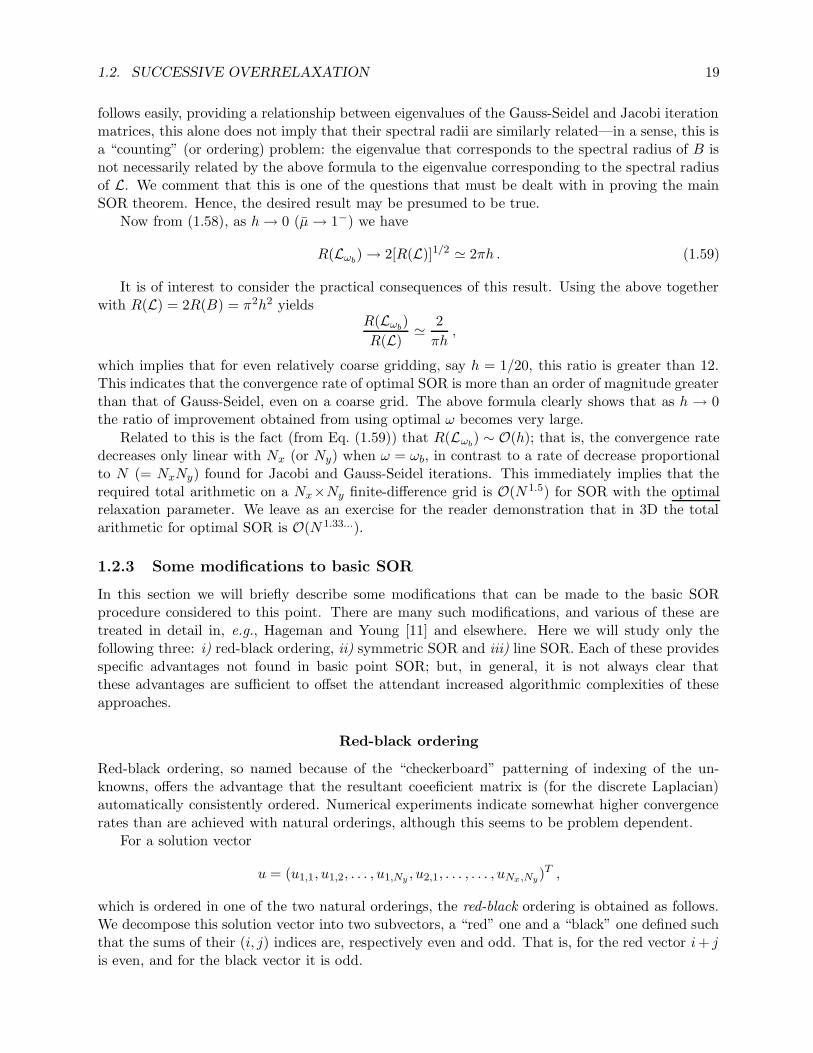
It is of value to consider a simple example to more clearly demonstrate this decomposition.The mesh shown in Fig. 1.9 includes the interior grid points corresponding to a Laplace-Dirichletproblem on the unit square for which a 5-point centered discretization with uniform grid spacingh = hx = hy = 1/6 has been constructed, and boundary-point indexing has been omitted. Hence,all equations will be of the form (1.54).
1,1
1,2
1,3
1,4
1,5
2,1
2,2
2,3
2,4
2,5
3,1
3,2
3,3
3,4
3,5
4,1
4,2
4,3
4,4
4,5
5,1
5,2
5,3
5,4
5,5
R
B
R R
RRR
R R R
B B
BBB
B B
B B
BB
R R
R R
1
2
3
4
5
6
7
8
9
10
11
12
13
14
15
16
17
18
19
20
21
22
23
24
25
Figure 1.9: Red-black ordering for discrete Laplacian.
In this figure, the usual indexing is shown below and to the right of each grid point; whetherthe grid point is red or black is indicated above and to the left of the point, and the single-indexordering of evaluation is provided above and to the right of each point. The natural ordering inthis case is
u = (u1,1, . . . , u1,5, u2,1, . . . , u2,5, . . . , . . . , u4,1, . . . , u4,5, u5,1, . . . , u5,5)T ,
and the corresponding red-black ordering is
u = (u1,1, u1,3, u1,5, u2,2, u2,4, u3,1, . . . , u5,1, . . . , u5,5︸ ︷︷ ︸red
,
black︷ ︸︸ ︷u1,2, u1,4, u2,1, u2,3, u2,5, . . . , . . . , u5,4)
T .
We leave as an exercise to the reader the geometric test of consistent ordering of the matrixcorresponding to this red-black vector. We also note that the programming changes to convert astandard SOR code to red-black ordering are relatively minor.
Symmetric SOR
We next briefly describe a modification to the basic SOR point iteration procedure known assymmetric SOR (SSOR). It is easily checked that the SOR iteration matrix Lω is not symmetric,even when the system matrix A is symmetric. Moreover, from the fact that the eigenvector of alinearly convergent iteration scheme corresponding to the dominant eigenvalue (the spectral radius,up to a sign) is precisely en, we expect convergence to be more rapid when the iteration matrix issymmetric in light of properties of the power method iteration procedure for finding the dominanteigenvector (see Isaacson and Keller [12]). The SOR procedure can be easily symmetrized bymerely reversing the order in which the equations are evaluated on each successive iteration. Morespecifically, the symmetric SOR matrix Sω which we will construct below can be shown to besimilar to a symmetric matrix (see [11]), and hence it will have the same eigenstructure.
1.2. SUCCESSIVE OVERRELAXATION 21
We develop the SSOR procedure as follows. First, recall that the fixed-point form of the usualSOR iteration procedure is Eq. (1.50):
u(n+1) = (I − ωD−1L)−1[ωD−1U + (1 − ω)I
]u(n) + ω(I − ωD−1L)−1D−1b .
We can define the backward procedure by interchanging the L and U triangular matrices. Thus,with Lω defined as
Lω ≡ (I − ωD−1L)−1[ωD−1U + (1 − ω)I
],
we can define the backward SOR matrix as
Uω ≡ (I − ωD−1U)−1[ωD−1L + (1 − ω)I
].
Then SSOR can be viewed as a two-step procedure carried out as follows. First calculate
u(n+ 12) = Lωu(n) + kω,F ,
wherekω,F = ω(I − ωD−1L)−1D−1b .
Then calculateu(n+1) = Uωu(n+ 1
2) + kω,B ,
withkω,B = ω(I − ωD−1U)−1D−1b .
Substitution of the first of these into the second yields
u(n+1) = Uω
(Lωu(n) + kω,F
)+ kω,B
= UωLωu(n) + Uωkω,F + kω,B
= Sωu(n) + kω , (1.60)
with Sω and kω having obvious definitions.These constructions are important for analysis of the method; but, as noted previously, efficient
implementations do not employ the SOR matrix. Hence, to implement SSOR we need only be ableto run the usual Do-loops both forward and backward.
It is interesting that point SSOR can be shown theoretically to converge twice as fast as does theusual point SOR. However, twice as much arithmetic is performed per iteration in SSOR, so thereis no advantage in this regard. It is thus argued that the main thing to be gained is symmetry ofthe iteration matrix, which can be of value when SSOR is used in conjunction with other iterativemethods such as conjugate gradient acceleration to be treated later.
Line SOR
From the standpoint of wide applicability, successive line overrelaxation (SLOR) is probably themust robust and often-used form of SOR. Its robustness stems from the “more implicit” constructionused for SLOR. All of the forms of SOR discussed to this point were implemented so as to obtainan updated solution value at a single point with each application of the iteration formula—hence,the terminology point SOR. In SLOR, as the name suggests, a complete grid line of solution valuesis computed, simultaneously, with each application of the iteration formula. Figure 1.10 depictsthis situation.
There are several features to note regarding the SLOR procedure. The first is that the meshstar for any individual grid point is the same as in the SOR case, as the figure indicates, since
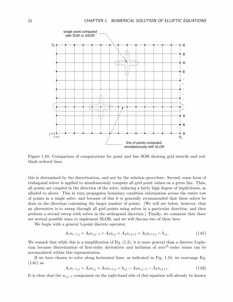
22 CHAPTER 1. NUMERICAL SOLUTION OF ELLIPTIC EQUATIONS
line of points computedsimultaneously with SLOR
single point computed with SOR or SSOR
i = 1j = 1
Nx
yN
R
B
R
.
.
.
.
.
.
.
B
R
B
R
Figure 1.10: Comparison of computations for point and line SOR showing grid stencils and red-black ordered lines.
this is determined by the discretization, and not by the solution procedure. Second, some form oftridiagonal solver is applied to simultaneously compute all grid point values on a given line. Thus,all points are coupled in the direction of the solve, inducing a fairly high degree of implicitness, asalluded to above. This in turn propagates boundary condition information across the entire rowof points in a single solve, and because of this it is generally recommended that these solves bedone in the direction containing the larger number of points. (We will see below, however, thatan alternative is to sweep through all grid points using solves in a particular direction, and thenperform a second sweep with solves in the orthogonal direction.) Finally, we comment that thereare several possible ways to implement SLOR, and we will discuss two of these here.
We begin with a general 5-point discrete operator,
A1ui−1,j + A2ui,j−1 + A3ui,j + A4ui,j+1 + A5ui+1,j = bi,j . (1.61)
We remark that while this is a simplification of Eq. (1.2), it is more general than a discrete Lapla-cian because discretization of first-order derivatives and inclusion of zeroth-order terms can beaccomodated within this representation.
If we have chosen to solve along horizontal lines, as indicated in Fig. 1.10, we rearrange Eq.(1.61) as
A1ui−1,j + A3ui,j + A5ui+1,j = bi,j − A2ui,j−1 − A4ui,j+1 . (1.62)
It is clear that the ui,j−1 component on the right-hand side of this equation will already be known

1.2. SUCCESSIVE OVERRELAXATION 23
at the current iteration level if we are traversing the lines in the direction of increasing j index. (Ifnot, then ui,j+1 will be known.) Thus, we can write the above as
A1u(n+1)i−1,j + A3u
(n+1)i,j + A5u
(n+1)i+1,j = bi,j − A2u
(n+1)i,j−1 − A4u
(n)i,j+1 , (1.63)
for each fixed j and i = 1, 2, . . . , Nx. For each such fixed j this is clearly a tridiagonal linear systemwhich can be solved by efficient sparse LU decompositions, or by cyclic reduction methods (seee.g., Birkhoff and Lynch [13]). In either case, O(Nx) arithmetic operations are needed for eachline, so O(N) total arithmetic is required for each iteration, just as in point SOR. As is fairly easyto determine, the arithmetic per line for SLOR is somewhat higher than for the usual point SORexcept when A is symmetric. For this special case (which arises, e.g., for Laplace-Dirichlet problems)Cuthill and Varga [14] have provided a numerically stable tridiagonal elimination requiring exactlythe same arithmetic per line as used in point SOR.
Before giving details of the implementation of SLOR we will first provide a brief discussionof further generalizations of SOR, usually termed “block” SOR, because SLOR is a special case.Extensive discussions can be found in Young [8] and Hageman and Young [11]. A brief descriptionsimilar to the treatment to be given here can be found in Birkhoff and Lynch [13].
Rather than consider a single line at a time, as we have done above, we might instead si-multaneously treat multiple lines (thus gaining even further implicitness) by defining subvectorsu1, u2, . . . , um of the solution vector u and writing the original system as
Au =
A11 A12 · · · A1m
A21 A22 · · · ......
. . ....
Am1 · · · · · · Amm
u1
u2...
um
=
b1
b2...
bm
. (1.64)
Here each Aii is a square nonsingular submatrix of A of size Ni×Ni such that∑m
i=1 Ni = N . IfNi = Nx or if Ni = Ny, then we obtain SLOR.
As noted in [13] it is possible to define block consistently-ordered and block property A analogousto our earlier definitions for point SOR. It is further noted in that reference that Parter [15] hasshown for k-line SOR applied to discrete equations corresponding to a Poisson equation on the unitsquare that the spectral radius of the SLOR iteration matrix is
ρ(L(k−line)ωb
) ' 1 − 2π√
2kh , (1.65)
and correspondingly, the asymptotic convergence rate is given by
R(L(k−line)ωb
) ' 2π√
2kh . (1.66)
Thus, typical single-line SLOR (k = 1) has a convergence rate that is a factor√
2 larger than thatof ordinary point SOR. We should also comment that because the block formalism is constructedin the same manner as is point SOR, and in addition because the block structure has no influenceon the Jacobi iteration matrix, the optimal parameter for such methods is expected to be the sameas for point SOR.
We are now prepared to consider two specific implementations of SLOR. The first is a directline-by-line application of Eq. (1.63). This is embodied in the following pseudo-language algorithm.
24 CHAPTER 1. NUMERICAL SOLUTION OF ELLIPTIC EQUATIONS
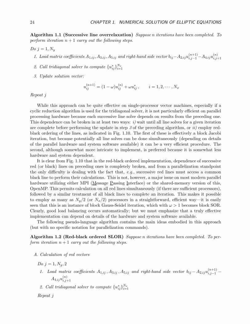
Algorithm 1.1 (Successive line overrelaxation) Suppose n iterations have been completed. Toperform iteration n + 1 carry out the following steps.
Do j = 1, Ny
1. Load matrix coefficients A1,ij , A3,ij , A5,ij and right-hand side vector bij−A2,iju(n+1)i,j−1 −A4,iju
(n)i,j+1
2. Call tridiagonal solver to compute u∗ijNx
i=1
3. Update solution vector:
u(n+1)ij = (1 − ω)u
(n)ij + ωu∗
ij , i = 1, 2, · · · , Nx
Repeat j
While this approach can be quite effective on single-processor vector machines, especially if acyclic reduction algorithm is used for the tridiagonal solver, it is not particularly efficient on parallelprocessing hardware because each successive line solve depends on results from the preceding one.This dependence can be broken in at least two ways: i) wait until all line solves for a given iterationare complete before performing the update in step 3 of the preceding algorithm, or ii) employ red-black ordering of the lines, as indicated in Fig. 1.10. The first of these is effectively a block Jacobiiteration, but because potentially all line solves can be done simultaneously (depending on detailsof the parallel hardware and system software available) it can be a very efficient procedure. Thesecond, although somewhat more intricate to implement, is preferred because it is somewhat lesshardware and system dependent.
It is clear from Fig. 1.10 that in the red-black ordered implementation, dependence of successivered (or black) lines on preceding ones is completely broken, and from a parallelization standpointthe only difficulty is dealing with the fact that, e.g., successive red lines must access a commonblack line to perform their calculations. This is not, however, a major issue on most modern parallelhardware utilizing either MPI (Message Passing Interface) or the shared-memory version of this,OpenMP. This permits calculation on all red lines simultaneously (if there are sufficient processors),followed by a similar treatment of all black lines to complete an iteration. This makes it possibleto employ as many as Ny/2 (or Nx/2) processors in a straightforward, efficient way—it is easilyseen that this is an instance of block Gauss-Seidel iteration, which with ω > 1 becomes block SOR.Clearly, good load balancing occurs automatically; but we must emphasize that a truly effectiveimplementation can depend on details of the hardware and system software available.
The following pseudo-language algorithm contains the main ideas embodied in this approach(but with no specific notation for parallelization commands).
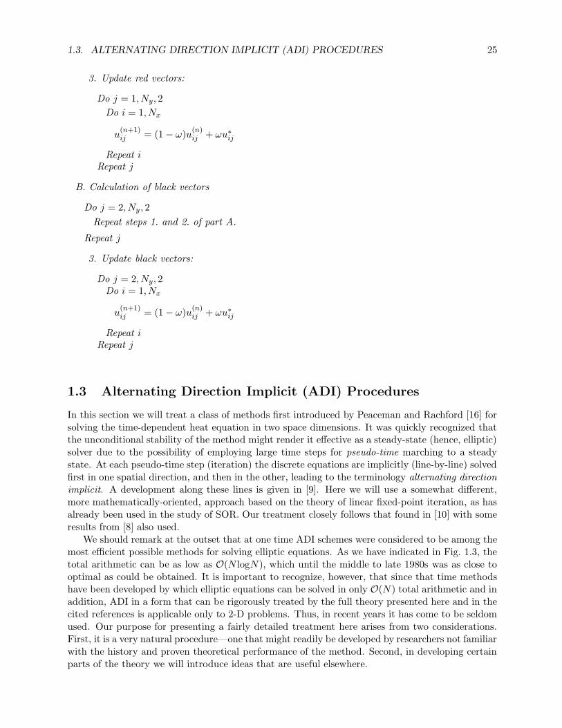
Algorithm 1.2 (Red-black ordered SLOR) Suppose n iterations have been completed. To per-form iteration n + 1 carry out the following steps.
A. Calculation of red vectors
Do j = 1, Ny , 2
1. Load matrix coefficients A1,ij , A3,ij , A5,ij and right-hand side vector bij −A2,iju(n+1)i,j−1 −
A4,iju(n)i,j+1
2. Call tridiagonal solver to compute u∗ijNx
i=1
Repeat j
1.3. ALTERNATING DIRECTION IMPLICIT (ADI) PROCEDURES 25
3. Update red vectors:
Do j = 1, Ny, 2
Do i = 1, Nx
u(n+1)ij = (1 − ω)u
(n)ij + ωu∗
ij
Repeat iRepeat j
B. Calculation of black vectors
Do j = 2, Ny , 2
Repeat steps 1. and 2. of part A.
Repeat j
3. Update black vectors:
Do j = 2, Ny, 2Do i = 1, Nx
u(n+1)ij = (1 − ω)u
(n)ij + ωu∗
ij
Repeat iRepeat j
1.3 Alternating Direction Implicit (ADI) Procedures
In this section we will treat a class of methods first introduced by Peaceman and Rachford [16] forsolving the time-dependent heat equation in two space dimensions. It was quickly recognized thatthe unconditional stability of the method might render it effective as a steady-state (hence, elliptic)solver due to the possibility of employing large time steps for pseudo-time marching to a steadystate. At each pseudo-time step (iteration) the discrete equations are implicitly (line-by-line) solvedfirst in one spatial direction, and then in the other, leading to the terminology alternating directionimplicit. A development along these lines is given in [9]. Here we will use a somewhat different,more mathematically-oriented, approach based on the theory of linear fixed-point iteration, as hasalready been used in the study of SOR. Our treatment closely follows that found in [10] with someresults from [8] also used.
We should remark at the outset that at one time ADI schemes were considered to be among themost efficient possible methods for solving elliptic equations. As we have indicated in Fig. 1.3, thetotal arithmetic can be as low as O(N logN), which until the middle to late 1980s was as close tooptimal as could be obtained. It is important to recognize, however, that since that time methodshave been developed by which elliptic equations can be solved in only O(N) total arithmetic and inaddition, ADI in a form that can be rigorously treated by the full theory presented here and in thecited references is applicable only to 2-D problems. Thus, in recent years it has come to be seldomused. Our purpose for presenting a fairly detailed treatment here arises from two considerations.First, it is a very natural procedure—one that might readily be developed by researchers not familiarwith the history and proven theoretical performance of the method. Second, in developing certainparts of the theory we will introduce ideas that are useful elsewhere.
26 CHAPTER 1. NUMERICAL SOLUTION OF ELLIPTIC EQUATIONS
There are three main topics associated with study of ADI in a mathematical context, and whichwe will treat in subsequent subsections. The first is convergence (and convergence rate) in the caseof using a constant iteration parameter (analogous to a pseudo-time step size), and selection ofan optimal parameter. Second is convergence for the case of variable iteration parameters (so-called cyclic ADI) and prediction of (nearly) optimal sequences of such parameters. Finally, wewill consider the “commutative” and “noncommutative” cases of ADI. This is important becausethe former occurs only in separable problems which can be solved analytically, or at least with afast Poisson solver. The noncommutative case, which therefore is more important for applications,unfortunately does not have the rigorous theoretical foundation of the commutative case. Never-theless, ADI tends to perform rather well, even for the more practical noncommutative problemsin two space dimensions.
1.3.1 ADI with a single iteration parameter
In this subsection we will begin by presenting the form of problem to be considered throughout thistreatment of ADI. We will see that it is slightly more restrictive than was the case for SOR, butrecall that our theory for SOR held rigorously only for 5-point (7-point in 3D) discrete operators.Following this we will derive the basic fixed-point iteration formula for single-parameter ADI, andthen state and prove a theorem regarding convergence of the iterations. We will then derive the op-timal parameter value for this iteration scheme and from this compute the asymptotic convergencerate for the method.
The form of the PDE to be studied in this section is
− (aux)x − (auy)y + su = f , (x, y) ∈ Ω , (1.67)
where Ω ⊂ R2 is a bounded rectangle. We will also assume that Dirichlet boundary conditions
are applied on all of ∂Ω, although we observe that the theory can be developed for other typicalboundary conditions. Also note that a, s and f may all be functions of (x, y).
When Eq. (1.67) is discretized in the usual way (see Chap. 3 for methods to discretize the self-adjoint form operators in this expression) with centered difference approximations the resultingsystem of linear algebraic equations takes the form
Au = b , (1.68)
which is again just Eq. (1.3). Thus, A has the structure of a discrete Laplacian, but it is notnecessarily constant coefficient.
ADI as a fixed-point iteration
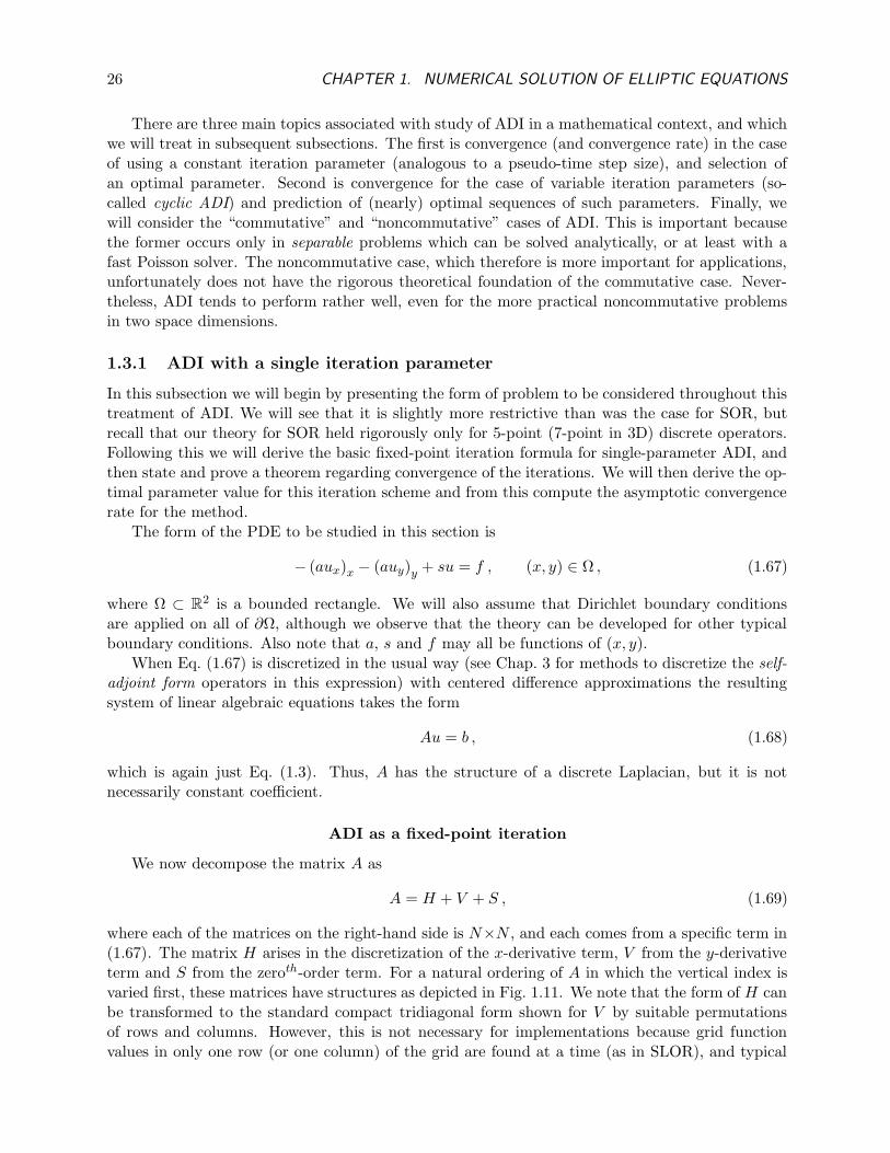
We now decompose the matrix A as
A = H + V + S , (1.69)
where each of the matrices on the right-hand side is N×N , and each comes from a specific term in(1.67). The matrix H arises in the discretization of the x-derivative term, V from the y-derivativeterm and S from the zeroth-order term. For a natural ordering of A in which the vertical index isvaried first, these matrices have structures as depicted in Fig. 1.11. We note that the form of H canbe transformed to the standard compact tridiagonal form shown for V by suitable permutationsof rows and columns. However, this is not necessary for implementations because grid functionvalues in only one row (or one column) of the grid are found at a time (as in SLOR), and typical
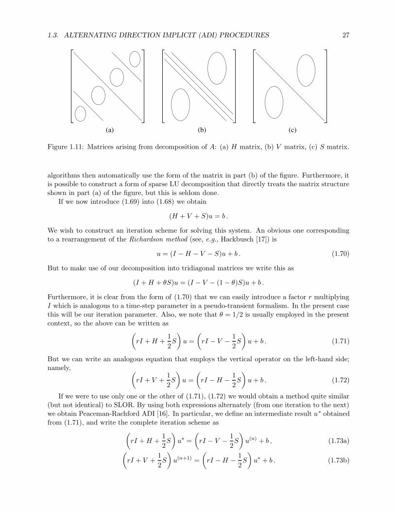
1.3. ALTERNATING DIRECTION IMPLICIT (ADI) PROCEDURES 27
(a) (b) (c)
Figure 1.11: Matrices arising from decomposition of A: (a) H matrix, (b) V matrix, (c) S matrix.
algorithms then automatically use the form of the matrix in part (b) of the figure. Furthermore, itis possible to construct a form of sparse LU decomposition that directly treats the matrix structureshown in part (a) of the figure, but this is seldom done.
If we now introduce (1.69) into (1.68) we obtain
(H + V + S)u = b .
We wish to construct an iteration scheme for solving this system. An obvious one correspondingto a rearrangement of the Richardson method (see, e.g., Hackbusch [17]) is
u = (I − H − V − S)u + b . (1.70)
But to make use of our decomposition into tridiagonal matrices we write this as
(I + H + θS)u = (I − V − (1 − θ)S)u + b .
Furthermore, it is clear from the form of (1.70) that we can easily introduce a factor r multiplyingI which is analogous to a time-step parameter in a pseudo-transient formalism. In the present casethis will be our iteration parameter. Also, we note that θ = 1/2 is usually employed in the presentcontext, so the above can be written as
(rI + H +
1
2S
)u =
(rI − V − 1
2S
)u + b . (1.71)
But we can write an analogous equation that employs the vertical operator on the left-hand side;namely, (
rI + V +1
2S
)u =
(rI − H − 1
2S
)u + b . (1.72)
If we were to use only one or the other of (1.71), (1.72) we would obtain a method quite similar(but not identical) to SLOR. By using both expressions alternately (from one iteration to the next)we obtain Peaceman-Rachford ADI [16]. In particular, we define an intermediate result u∗ obtainedfrom (1.71), and write the complete iteration scheme as
(rI + H +
1
2S
)u∗ =
(rI − V − 1
2S
)u(n) + b , (1.73a)
(rI + V +
1
2S
)u(n+1) =
(rI − H − 1
2S
)u∗ + b . (1.73b)

28 CHAPTER 1. NUMERICAL SOLUTION OF ELLIPTIC EQUATIONS
It can readily be seen from the pseudo-transient viewpoint that this scheme is convergent forand r > 0 due to the unconditional stability of the Crank-Nicolson method to which it is equivalent.We will prove this here in a different manner, making use of the theory of linear fixed-point iterationas we have done for SOR, because this will lead us to a formula for optimal r. This is not availablefrom analysis of the pseudo-transient formalism. We also note that consistency of Eqs. (1.73) withthe original PDE follows directly from the construction of Eq. (1.70). This too is more difficult toobtain from a pseudo-transient analysis.
Convergence of ADI iterations
We begin study of convergence of ADI by defining matrices to simplify notation:
H1 ≡ H +1
2S , V1 ≡ V +
1
2S ,
and write Eqs. (1.73) as
(rI + H1)u∗ = (rI − V1)u
(n) + b ,
(rI + V1)u(n+1) = (rI − H1)u
∗ + b .
Formal solution of these equations followed by substitution of the former into the latter yields
u(n+1) = (rI + V1)−1(rI − H1)
(rI + H1)
−1[(rI − V1)u
(n) + b]
+ (rI + V1)−1b ,
oru(n+1) = Tru
(n) + kr , (1.74)
whereTr ≡ (rI + V1)
−1(rI − H1)(rI + H1)−1(rI − V1) (1.75)
is the Peaceman-Rachford iteration matrix, and
kr ≡ (rI + V1)−1[(rI − H1)(rI + H1)
−1 + I]b . (1.76)
We see that (1.74) is of exactly the same form as all of the basic iteration schemes considered sofar, now with G = Tr.
Thus, we would expect that to study convergence of the iterations of (1.74) we need to estimateρ(Tr). To do this we first use a similarity transformation to define
Tr ≡ (rI + V1)Tr(rI + V1)−1
= (rI − H1)(rI + H1)−1(rI − V1)(rI + V1)
−1 ,
which is similar to Tr and thus has the same spectral radius. Hence, we have
ρ(Tr) = ρ(Tr) ≤ ‖Tr‖≤ ‖(rI − H1)(rI + H1)
−1‖‖(rI − V1)(rI + V1)−1‖ .
We can now state the basic theorem associated with single-parameter ADI iterations.
1.3. ALTERNATING DIRECTION IMPLICIT (ADI) PROCEDURES 29
Theorem 1.10 Let H1 and V1 be N ×N Hermitian non-negative definite matrices with at leastone being positive definite. Then ρ(Tr) < 1 ∀ r > 0.
Proof. Since H1 is Hermitian its eigenvalues are real, and H1 is diagonalizable. The same is truefor rI − H1 and rI + H1. Moreover, since H1 is non-negative definite, λj ≥ 0 holds ∀ λj ∈ σ(H1).Now if λj ∈ σ(H1) it follows that r−λj ∈ σ(rI −H1), and r +λj ∈ σ(rI +H1). Furthermore, sincerI + H1 is diagonalizable, (r + λj)
−1 ∈ σ((rI + H1)
−1). Finally, it follows from this and a direct
calculation that the eigenvalues of (rI − H1)(rI + H1)−1 are (r − λj)/(r + λj). Thus, taking ‖ · ‖
to be the spectral norm leads to
‖(rI − H1)(rI + H1)−1‖ = max
1≤j≤N
∣∣∣∣r − λj
r + λj
∣∣∣∣ .
Clearly, the quantity on the right is less than unity for any λj > 0 and ∀ r > 0. The same argumentsand conclusions apply for ‖(rI − V1)(rI + V1)
−1‖, completing the proof.
ADI optimal parameter
We now consider the problem of choosing an optimal parameter value r for the ADI iterations.In the context of a pseudo-transient formalism, and in light of the manner in which r enters theiteration formulas, e.g., (1.73), we would expect r to be rather small since it is roughly the reciprocalof the pseudo-time step. In principle this would seem to produce the fastest convergence to steadystate.
To permit a direct comparison of convergence rate (to be obtained as part of the optimalparameter analysis) with results obtained earlier for SOR, we restrict attention to the Laplace-Dirichlet problem. But we emphasize, as remarked above, that the analyses presented here can beconducted for somewhat more general problems; we leave this as an exercise for the reader.
We will employ a uniform grid in both directions on the unit square so that Nx = Ny, leading tohx = hy = h = 1/(Nx − 1). We will also assume that the Dirichlet conditions have been eliminatedfrom the discrete equations resulting in only Nx − 2 points in each direction at which solutions aresought. This implies that the system matrix A will be of size (Nx − 2)2, and correspondingly thisnumber of eigenvectors will be needed to span the space on which this matrix acts.
Now suppose that α(k,`) is one such eigenvector, and that its (i, j)th component can be repre-sented as
α(k,`)i,j = γk,` sin
((k − 1)(i − 1)π
Nx − 1
)sin
((` − 1)(j − 1)π
Nx − 1
), (1.77)
2 ≤ i, j ≤ Nx − 1 , 2 ≤ k, ` ≤ Nx − 1 .
Here, γk,` is a constant that can ultimately be determined via normalization, but in analyses suchas presented here, it actually cancels.
If we form the eigenvalue problems for H1 and V1 and substitute α(k,`)i,j for the eigenvector, we
can easily show that the eigenvalues of H1 (= H in this case) are
λk = 2 − 2 cos
((k − 1)π
Nx − 1
)k = 2, 3, . . . , Nx − 1 , (1.78)
and those of V1 are
λ` = 2 − 2 cos
((` − 1)π
Nx − 1
)` = 2, 3, . . . , Nx − 1 . (1.79)
30 CHAPTER 1. NUMERICAL SOLUTION OF ELLIPTIC EQUATIONS
We note here that the choice of Eq. (1.77) for the form of the eigenvector component is motivatedin the same way is in the Jacobi iteration analysis done earlier.
We can use a trigonometric identity to express these as, for example,
λk = 4 sin2
((k − 1)π
2(Nx − 1)
).
It then follows that the eigenvalues of the Peaceman-Rachford iteration matrix Tr are
λk,` =
r − 4 sin2(
(k−1)π2(Nx−1)
)
r + 4 sin2(
(k−1)π2(Nx−1)
)
r − 4 sin2(
(`−1)π2(Nx−1)
)
r + 4 sin2(
(`−1)π2(Nx−1)
)
, (1.80)
and from this we see (for our special case of Nx = Ny and uniform h) that
ρ(Tr) =
max
2≤k≤Nx−1
∣∣∣∣∣∣
r − 4 sin2(
(k−1)π2(Nx−1)
)
r + 4 sin2(
(k−1)π2(Nx−1)
)
∣∣∣∣∣∣
2
. (1.81)
We leave as an exercise to the reader derivation of the analogous formula for the more general cases.We now want to choose r so as to minmize ρ(Tr). To do this we consider the function
g(ξ, r) =r − ξ
r + ξ, r > 0 , ξ ∈ [ξ1, ξ2] ,
for ξ1 > 0. For the given r and ξ intervals, a direct calculation (left as an exercise for the reader)shows that ∂g/∂ξ < 0, strictly; so g is monotone decreasing. Thus, max |g| occurs at one of theendpoints of the ξ interval. That is
maxξ∈[ξ1,ξ2]
|g(ξ, r)| = max
[∣∣∣∣r − ξ1
r + ξ1
∣∣∣∣ ,∣∣∣∣r − ξ2
r + ξ2
∣∣∣∣]
(1.82)
for each fixed r. Using this, it is easily checked that
maxξ∈[ξ1,ξ2]
|g(ξ, r)| =
ξ2−rξ2+r 0 < r ≤ √
ξ1ξ2
r−ξ1r+ξ1
r ≥ √ξ1ξ2 .
(1.83)
This provides an expression for ρ(Tr) as a function only of r, and a direct calculation shows that
minr>0
maxξ∈[ξ1,ξ2]
|g(ξ, r)| =1 −
√ξ1/ξ2
1 +√
ξ1/ξ2
, (1.84)
which implies (upon multiplying the numerator and the denominator by ξ2) that
ropt =√
ξ1ξ2 . (1.85)
Now recall from the definition of g(ξ, r) and the form of ρ(Tr) that [ξ1, ξ2] is the spectral intervalfor the eigenvalues in each direction for the given problem. Thus, in the present case we have
ξ1 = 4 sin2
(π
2(Nx − 1)
)= 4 sin2
(π
2h)
(1.86)
1.3. ALTERNATING DIRECTION IMPLICIT (ADI) PROCEDURES 31
and
ξ2 = 4 sin2
((Nx − 2)π
2(Nx − 1)
)= 4 cos2
(π
2(Nx − 1)
)= 4 cos2
(π
2h)
(1.87)
We can now substitute these into Eq. (1.85) to obtain an explicit expression for the optimaliteration parameter value in terms of the spatial step size:
ropt = 4 sin(π
2h)
cos(π
2h)
. (1.88)
In the limit h → 0 this is approximately 2πh, which is small; so our intuition regarding the size ofpseudo-time steps is roughly correct.
We can also use the above values of the ξs in (1.84) to find that
minr>0
ρ(Tr) =
[1 − tan
(π2 h)
1 + tan(
π2 h)]2
,
which can be rearranged to yield
ρ(Tr) =1 − 2 sin π
2 h cos π2 h
1 + 2 sin π2 h cos π
2 h(1.89)
for optimal iteration parameter r. One can check that for small h (neglecting O(h3) terms) we have
ρ(Tr) '1 − πh
1 + πh' 1 − 2πh + O(h2) . (1.90)
But since log(1 − 2πh) ∼= −2πh for sufficiently small h, it follows from the definition of asymptoticconvergence rate that R(Tr) ∼= 2πh for optimal r; this is precisely the same result obtained foroptimal SOR. But one must recognize that the amount of work per iteration is greater by morethan a factor of two for ADI; indeed, it is almost exactly a factor of two greater than that requiredby SLOR—which has a higher convergence rate, and can be extended to the 3-D case in a naturalway. We see from this why Peaceman-Rachford ADI is no longer widely used, despite its ratherinuitively appealing traits.
1.3.2 ADI: the commutative case
In this section we will outline the analysis of Peaceman-Rachford ADI for the special case whenH1V1 = V1H1. We will see that under this assumption (and not otherwise, in general) it is possi-ble to generate (nearly) optimal sequences of iteration parameters whose use embodies the cyclicADI procedures. We will see that these nonstationary iteration methods (ones whose iterationparameters change from one iteration to the next) are significantly more efficient than is the single-parameter version discussed in the preceding section. We will begin the treatment with the basiciteration formula construction followed by a major theorem associated with such procedures. Wewill then sketch the process of determining the optimal parameter sequences and give two widely-used specific examples of these.
Cyclic ADI iteration formula
We begin by noting that since ρ(Tr) < 1 ∀ r > 0 in our single-parameter formulation of ADI, thereis no reason to use a single parameter in Eqs. (1.73). Thus, in place of these equations we here
32 CHAPTER 1. NUMERICAL SOLUTION OF ELLIPTIC EQUATIONS
consider
(rn+1I + H1)u∗ = (rn+1I − V1)u
(n) + b , (1.91a)
(rn+1I + V1)u(n+1) = (rn+1I − H1)u
∗ + b . (1.91b)
In fact, we could even use different values of r in the individual steps of these equations, as mightalso have been done in the stationary iteration procedure of the previous section (see, e.g., Axelsson[18] for an example of this).
After n iterations of this procedure the corresponding representation of the iteration matrix is
n∏
k=1
Trk,
rather than simply T nr as would be the case for the stationary single-parameter case. Intuitively,
we would expect
ρ
(n∏
k=1
Trk
)< 1 ∀ n ≥ 1
since we have shown that ρ(Tr) < 1 ∀ r > 0. But this is a naive expectation, and there are subtletiesthat prevent proving such a result. In fact, counterexamples for which convergence does not occurcan be found when the matrices H1 and V1 do not commute (see [8]). To guarantee convergence itis necessary that the same orthonormal basis of eigenvectors spans the eigenspace of both H1 andV1. In this case, the following theorem can be proven (see Varga [10]).
Theorem 1.11 Let H1 and V1 be N×N Hermitian positive definite matrices with H1V1 = V1H1.Then for any set rkn
k=1 of positive real numbers we have
∥∥∥∥∥
n∏
k=1
Trk
∥∥∥∥∥ = ρ
(n∏
k=1
Trk
)= max
1<i,j≤N
n∏
k=1
∣∣∣∣rk − σi
rk + σi
∣∣∣∣∣∣∣∣rk − τj
rk + τj
∣∣∣∣ < 1 , (1.92)
where σi ∈ σ(H1), τj ∈ σ(V1). Moreover, if rn+1 > 0, then
∥∥∥∥∥
n+1∏
k=1
Trk
∥∥∥∥∥ <
∥∥∥∥∥
n∏
k=1
Trk
∥∥∥∥∥ .
The norm in (1.92) and following is the spectral norm.
The last inequality above implies that the error is decreased by increasing amounts for eachsucceeding iteration within a parameter sequence. In fact, if σ(H1) and σ(V1) were completelyknown, it would be possible to construct a direct (non-iterative) solution procedure by choosingan appropriate sequence rkn
k=1. We remark that this also occurs for Chebychev acceleration (nottreated herein, but see e.g., [18]), and it is our first indication that cyclic ADI represents a significantimprovement over the single-parameter version.
In general, we seldom have available the complete spectra for H1 and V1. There are, howevertechniques whereby we can obtain bounds on the eigenvalues, leading to useful approximations ofthe parameter sets rkn
k=1. In particular, it is often possible to estimate α and β such that
0 < α ≤ σi, τj ≤ β , i, j = 1, 2, . . . , N .
1.3. ALTERNATING DIRECTION IMPLICIT (ADI) PROCEDURES 33
Then we have
max1≤i,j≤N
n∏
k=1
∣∣∣∣rk − σi
rk + σi
∣∣∣∣∣∣∣∣rk − τj
rk + τj
∣∣∣∣ ≤[
max1≤i≤N
n∏
k=1
∣∣∣∣rk − σi
rk + σi
∣∣∣∣
]·[
max1≤j≤N
n∏
k=1
∣∣∣∣rk − τj
rk + τj
∣∣∣∣
]
≤
max
ξ∈[α,β]
n∏
j=1
∣∣∣∣rj − ξ
rj + ξ
∣∣∣∣
2
.
From this it follows that ∥∥∥∥∥∥
n∏
j=1
Trj
∥∥∥∥∥∥≤[
maxξ∈[α,β]
|gn(ξ, r)|]2
,
where
gn(ξ, r) ≡n∏
j=1
(rj − ξ
rj + ξ
).
It is clear that this is now in the same form as that treated earlier in the single-parameter case,and analogous to what was done there, we now seek a set of rjs that will minimize the maximum of|gn| with respect to ξ ∈ [α, β]. We remark that the exact solution to this min-max problem is notknown in general; however, when n = 2k for any k ≥ 0, Wachspress [19] has provided an elegantexact result, as described in [10]. Here, we will present results from an approximate solution tothis problem in the form of “nearly” optimal rjs as well as the required number of them—all as afunction of α, β and the mesh size h.
To begin, we divide the spectral interval [α, β] into n subintervals (noting that n has not as yetbeen prescribed) such that
α = ξ0 < ξ1 < ξ2 < · · · < ξn = β .
Then on each of these subintervals we consider the one-parameter min-max problem
minrj
[max
ξ∈[ξj−1,ξj ]
∣∣∣∣rj − ξ
rj + ξ
∣∣∣∣]
,
which is identical to the single-parameter problem of the preceding section, except that it is posedon only a subset of the spectral interval. Hence, we already know the solution to this problem isrj =
√ξj−1ξj for each jth subinterval. Our task now is to find the ξjs and n, the number of rjs.
First, analogous to Eq. (1.84) we have
minrj
[max
ξ∈[ξj−1,ξj ]
∣∣∣∣rj − ξ
rj + ξ
∣∣∣∣]
=1 −
√ξj−1/ξj
1 −√
ξj−1/ξj
≡ δ (1.93)
Now define
γ ≡(
β
α
) 12n
, (1.94)
and set
δ =γ − 1
γ + 1. (1.95)
The last of these arises naturally by factoring√
ξj−1/ξj from both numerator and denominator of(1.93), and then with n = 1 setting ξj−1 = α and ξj = β.
34 CHAPTER 1. NUMERICAL SOLUTION OF ELLIPTIC EQUATIONS
We can now use these formulas recursively to find the ξjs and then the rjs. In particular, fromeq93:ch1, if n 6= 1 but is known and the spectral interval bounds are known, then we can calculateδ and starting with j = 1 (for which ξj−i = ξ0 = α is known), we can solve for ξ1. Then werecursively apply this procedure to find the remaining ξjs. It is is possible to derive a very simpleformula that accomplishes this directly:
ξj = αγ2j . (1.96)
We leave this derivation as an exercise for the reader.
The only remaining unknown associated with the sequence of iteration parameters is the numberof them, n. This is derived in [10], and here we will only give the result; but we note that the basicidea underlying the derivation is to choose n so as to maximize the average convergence rate overa cycle of length n. This leads to the formula
n ≥ 1
2
ln(
βα
)
ln(
1√2−1
) . (1.97)
We can now find the (nearly) optimal parameter sequence using the formula
rj = αγ2j−1 , j = 1, 2, . . . , n , (1.98)
which follows directly from rj =√
ξj−1/ξj . This sequence is due to Peaceman and Rachford [16].There are numerous similar sequences, derived via modifications of the technique outlined above.One of the more successful ones is due to Wachspress [19]:
n ≥ 1 +1
2
ln(
βα
)
ln(
1√2−1
) , (1.99)
and
rj = β
(α
β
)(j−1)/(n−1)
, j = 1, 2, . . . , n , (1.100)
In both of these expressions for n, the right-hand side will obviously not produce an integer result.But Theorem 1.11 suggests that longer sequences are preferred to shorter ones; so the rule is to usethe first integer larger than the decimal number produced by the formula.
There is one final calculation that must be demonstrated before it is possible to actually producethe above iteration parameters. It is the determination of α and β. The approach is actuallyequivalent to what we did earlier in the single parameter case, but we will present it somewhatmore formally here.
Theorem 1.12 Let A be a (N − 2)×(N − 2) tridiagonal matrix arising from discretization of aLaplace-Dirichlet problem on a grid of uniform spacing h = 1/(N − 1). Let the main diagonalof A consist of the nonzero elements a and the two off-diagonals contain elements b. Then theeigenvalues of A are
λj = a + 2b cos((j − 1)πh) , j = 2, 3, . . . , N − 1 . (1.101)
1.4. INCOMPLETE LU DECOMPOSITION (ILU) 35
The proof of this is the same as the construction employed earlier for eignenvalues of the Jacobiiteration matrix.
Mitchell and Griffiths [9] state, without proof, the following result for eigenvalues of nonsym-metric matrices.
λj = a + 2√
bc cos((j − 1)πh) , (1.102)
where b and c are off-diagonal elements, and the rest of the problem statement is the same as inthe theorem above.
1.3.3 ADI: the noncommutative case
In the preceding section it was necessary to use the assumption H1V1 = V1H − 1 in order to proveconvergence of cyclic ADI, and we recall that it was mentioned that ADI may not converge withoutsatisfaction of this requirement. In this section we will briefly consider under what conditions thiscommutativity assumption can be expected to hold. All of our detailed analyses to this point haveinvolved the relatively simple Laplace-Dirichlet problem. We will now return to Eq. (1.67) whichwe here generalize slightly and write as
−(a1(x, y)ux)x − (a2(x, y)uy)y + s(x, y)u = f(x, y) , (x, y) ∈ Ω ⊂ R2 ,
with Dirichlet conditionsu(x, y) = g(x, y) , (x, y) ∈ ∂Ω .
It will be assumed that a1, a2 ∈ C1(Ω), a1, a2, s ∈ C(Ω), and a1, a2, s > 0 in Ω. The followingtheorem is the main result on commutativity with respect to ADI procedures.
Theorem 1.13 Let a1, a2 and s be as above. Then except for the case a1(x, y) = ϕ1(x), a2(x, y) =ϕ2(y), s(x, y) ≡ const. and Ω a rectangle, the matrices H1 and V1 fail to commute.
This is a well-known result; the proof can be found in [8] and [10], for example, and we will notrepeat it here. It is clear from this that the entire theory of cyclic ADI no longer holds in mostpractical cases. In particular, even if we begin with a constant-coefficient problem on a nonrectan-gular domain, by the time a coordinate transformation is performed to obtain a rectangular domain(see Chap. 4 for discussions of this), as required by the theorem, we will in general no longer havethe “separable” coefficients that are required.
This, and the fact that ADI does not have a natural extension to 3-D problems, makes itdifficult to recommend its use. As stated at the beginning of this section, our main goal herehas been to provide sufficient information on this rather natural approach to prevent its being re-invented. Indeed, even if the commutativity problem were not so severe, the O(N logN) arithmeticrequired by cyclic ADI still is more than needed for modern methods such as multigrid and domaindecomposition.
1.4 Incomplete LU Decomposition (ILU)
In this section we will treat a class of methods that at one time appeared to show great promisefor solving elliptic PDEs, especially in the context of practical engineering problems. However,as more demanding problems were attempted, especially when using highly-refined gridding, itbecame apparent that the method had no better convergence rate than either point SOR or single-parameter ADI, although it was typically more robust; but it required significantly more arithmetic

36 CHAPTER 1. NUMERICAL SOLUTION OF ELLIPTIC EQUATIONS
per iteration. With the increased understanding that has accumulated in recent years, it is evidentthat incomplete LU decompositions (ILUs) are useful mainly as preconditioners (to be discussed inthe next section) of other iterative techniques. They should generally not be used as “stand-alone”solvers.
In what follows we will begin with a basic general treatment of ILUs. Following this we will pro-vide details for the first (and probably best-known in the engineering literature) of these methods.We remark that there are many variants of what we will present. For a rather different approach,but embodying the same basic ideas, the reader is referred to Manteuffel [20] and Van der Voorst[21]; also see [17] and [18].
1.4.1 Basic ideas of ILU decomposition
We first observe that all of the methods we have considered up to this point could, in a generalway, be classified as ILUs. But as will be evident as we proceed, most would be rather trivialin this context and they are not usually included within the present framework. The basic ideasunderlying construction of ILUs are as follows.
Suppose we wish to solve the linear system Eq. (1.3) repeated here as
Au = b , (1.103)
where A is a sparse banded (but not compactly) N ×N nonsingular matrix. Because A is notcompactly banded, at least O(N 2) arithmetic operations would be required by an eliminationprocedure, and if standard methods (e.g., Gaussian elimination) are employed O(N 3) operationswould be needed. Moreover, O(N 2) words of storage would be necessary to handle the fill-inbetween bands during the elimination process.
We can avoid both the arithmetic and storage problems by replacing A with a matrix M thatis “nearly as sparse” as A, but which admits a sparse LU decomposition. In particular, we set
M = A + E , (1.104)
where E is an error (sometimes termed “defect”) matrix. Then the original system (1.103) can bewritten as
(M − E)u = b
or
Mu = Eu + b ,
which immediately suggests the fixed-point form
Mu(n+1) = Eu(n) + b . (1.105)
Now since M has a LU decomposition, we can express the above as
LUu(n+1) = Eu(n) + b ,
or
u(n+1) = U−1L−1Eu(n) + U−1L−1b . (1.106)
Clearly, this is in our standard linear fixed-point form
u(n+1) = Gu(n) + k ,
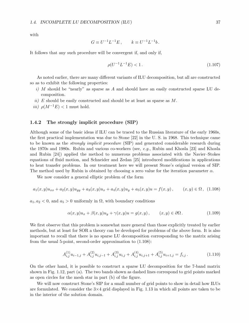
1.4. INCOMPLETE LU DECOMPOSITION (ILU) 37
with
G ≡ U−1L−1E , k ≡ U−1L−1b .
It follows that any such procedure will be convergent if, and only if,
ρ(U−1L−1E) < 1 . (1.107)
As noted earlier, there are many different variants of ILU decomposition, but all are constructedso as to exhibit the following properties:
i) M should be “nearly” as sparse as A and should have an easily constructed sparse LU de-composition.
ii) E should be easily constructed and should be at least as sparse as M .
iii) ρ(M−1E) < 1 must hold.
1.4.2 The strongly implicit procedure (SIP)
Although some of the basic ideas if ILU can be traced to the Russian literature of the early 1960s,the first practical implementation was due to Stone [22] in the U. S. in 1968. This technique cameto be known as the strongly implicit procedure (SIP) and generated considerable research duringthe 1970s and 1980s. Rubin and various co-workers (see, e.g., Rubin and Khosla [23] and Khoslaand Rubin [24]) applied the method to numerous problems associated with the Navier–Stokesequations of fluid motion, and Schneider and Zedan [25] introduced modifications in applicationsto heat transfer problems. In our treatment here we will present Stone’s original version of SIP.The method used by Rubin is obtained by choosing a zero value for the iteration parameter α.
We now consider a general elliptic problem of the form
a1(x, y)uxx + a2(x, y)uyy + a3(x, y)ux + a4(x, y)uy + a5(x, y)u = f(x, y) , (x, y) ∈ Ω , (1.108)
a1, a2 < 0, and a5 > 0 uniformly in Ω, with boundary conditions
α(x, y)ux + β(x, y)uy + γ(x, y)u = g(x, y) , (x, y) ∈ ∂Ω . (1.109)
We first observe that this problem is somewhat more general than those explicitly treated by earliermethods, but at least for SOR a theory can be developed for problems of the above form. It is alsoimportant to recall that there is no sparse LU decomposition corresponding to the matrix arisingfrom the usual 5-point, second-order approximation to (1.108):
A(1)i,j ui−1,j + A
(2)i,j ui,j−1 + A
(3)i,j ui,j + A
(4)i,j ui,j+1 + A
(5)i,j ui+1,j = fi,j . (1.110)
On the other hand, it is possible to construct a sparse LU decomposition for the 7-band matrixshown in Fig. 1.12, part (a). The two bands shown as dashed lines correspond to grid points markedas open circles for the mesh star in part (b) of the figure.
We will now construct Stone’s SIP for a small number of grid points to show in detail how ILUsare formulated. We consider the 3×4 grid displayed in Fig. 1.13 in which all points are taken to bein the interior of the solution domain.
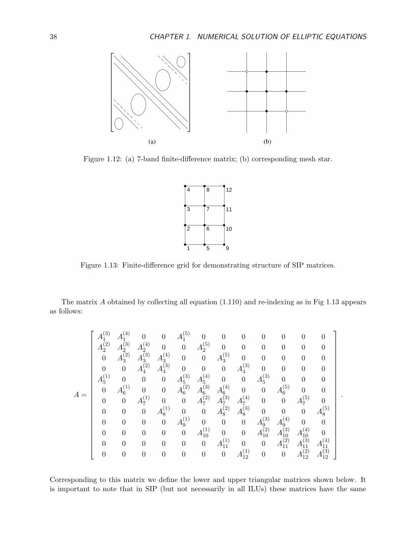
38 CHAPTER 1. NUMERICAL SOLUTION OF ELLIPTIC EQUATIONS
(a) (b)
Figure 1.12: (a) 7-band finite-difference matrix; (b) corresponding mesh star.
1
2
3
4
5
6
7
8
9
10
11
12
Figure 1.13: Finite-difference grid for demonstrating structure of SIP matrices.
The matrix A obtained by collecting all equation (1.110) and re-indexing as in Fig 1.13 appearsas follows:
A =
A(3)1 A
(4)1 0 0 A
(5)1 0 0 0 0 0 0 0
A(2)2 A
(3)2 A
(4)2 0 0 A
(5)2 0 0 0 0 0 0
0 A(2)3 A
(3)3 A
(4)3 0 0 A
(5)3 0 0 0 0 0
0 0 A(2)4 A
(3)4 0 0 0 A
(3)4 0 0 0 0
A(1)5 0 0 0 A
(3)5 A
(4)5 0 0 A
(3)5 0 0 0
0 A(1)6 0 0 A
(2)6 A
(3)6 A
(4)6 0 0 A
(5)6 0 0
0 0 A(1)7 0 0 A
(2)7 A
(3)7 A
(4)7 0 0 A
(5)7 0
0 0 0 A(1)8 0 0 A
(2)8 A
(3)8 0 0 0 A
(5)8
0 0 0 0 A(1)9 0 0 0 A
(3)9 A
(4)9 0 0
0 0 0 0 0 A(1)10 0 0 A
(2)10 A
(3)10 A
(4)10 0
0 0 0 0 0 0 A(1)11 0 0 A
(2)11 A
(3)11 A
(4)11
0 0 0 0 0 0 0 A(1)12 0 0 A
(2)12 A
(3)12
.
Corresponding to this matrix we define the lower and upper triangular matrices shown below. Itis important to note that in SIP (but not necessarily in all ILUs) these matrices have the same

1.4. INCOMPLETE LU DECOMPOSITION (ILU) 39
structure as the corresponding part of the original matrix.
L =
d1 0 0 · · · · · · · · · · · · · · · · · · · · · 0 0c2 d2 0 0 · · · · · · · · · · · · · · · · · · 0 0
0 c3 d3. . .
. . ....
...
0. . . c4 d4
. . .. . .
......
b5. . .
. . . c5 d5. . .
. . ....
...
0 b6. . .
. . . c6 d6. . .
. . ....
...... 0 b7
. . .. . . c7 d7
. . .. . .
......
......
. . . b8. . .
. . . c8 d8. . .
. . ....
......
.... . . b9
. . .. . . c9 d9
. . . 0 0...
.... . . b10
. . .. . . c10 d10 0 0
0 0 · · · · · · · · · 0 b11. . .
. . . c11 d11 00 0 · · · · · · · · · · · · 0 b12 0 0 c12 d12
,
and
U =
1 e1 0 0 f1 0 · · · · · · · · · · · · 0 00 1 e2 0 0 f2 0 · · · · · · · · · 0 0
0 0 1 e3 0 0 f3. . .
......
... 0. . . 1 e4 0 0 f4
. . ....
......
.... . .
. . . 1 e5 0 0 f5. . .
......
......
. . .. . . 1 e6 0 0 f6 0
......
.... . .
. . . 1 e7 0 0 f7 0...
.... . .
. . . 1 e8 0 0 f8...
.... . .
. . . 1 e9 0 0...
.... . . 0 1 e10 0
0 0 · · · · · · · · · · · · · · · · · · 0 0 1 e11
0 0 · · · · · · · · · · · · · · · · · · · · · 0 0 1
.
We now construct the product LU and compare its structure with that of the original matrixA. As expected, we find the two matrices have the same band structure except for two additionalbands immediately inside the outer bands in the LU product. In particular, the structure of this
40 CHAPTER 1. NUMERICAL SOLUTION OF ELLIPTIC EQUATIONS
matrix is the same as that indicated in Fig. 1.12 part (a).
LU =
d1 d1e1 0 0 d1f1 0 0 0 · · ·c2 d2 + c2e1 d2e2 0 c2f1 d2f2 0 0 · · ·0 c3 d3 + c3e2 d3e3 0 c3f2 d3f3 0 · · ·0 0 c4 d4 + c4e3 d4e4 0 c4f3 d4f4
. . .
b5 b5e1 0 c5 d5 + c5e4 + b5f1 d5e5 0 c5f4. . .
0 b6 b6e2 0 c6. . .
. . . 0. . .
... 0 b7 b7e3. . .
. . .. . .
. . .. . .
...... 0 b8 b8e4
. . .. . .
. . .. . .
......
... 0 b9 b9e5. . .
. . .. . .
.
We can now determine the elements of L and U by matching components of LU with those ofA. First, it is clear that
bi = A(1)i , ∀ i = 5, . . . , 12 ,
ci = A(2)i , ∀ i = 2, . . . , 12 .
Then
d1 = A(3)1 ,
and
e1 = A(4)1 /d1 , f1 = A
(5)1 /d1 .
Next, we find
d2 + c2e1 = A(3)2 ⇒ d2 = A
(3)2 − c2e1 .
In general, the dis are given by
di = A(3)i − ciei−1 − bifi−Ny ,
where, as usual, Ny is the number of points in the y direction. (Note that if we had used row-wisenatural ordering, rather than the column-wise ordering employed here, Ny would be replaced withNx.) The third term in this expression should be evaluated only for i > Ny. With this generalformula for di we are now able to calculate the remaining matrix elements, namely, those of thematrix U :
ei = A(4)i /di , fi = A
(5)i /di .
Once all of the elements of L and U have been evaluated, the elements of the error matrix can beconstructed. These are given by
E(1)i = biei−Ny and E
(2)i = cifi−1 .
We now observe that the difference equation (1.110) must be replaced with
A(1)i ui−Ny + E
(1)i ui−Ny+1 + A
(2)i ui−1 + A
(3)i ui + A
(4)i ui+1 + E
(2)i ui+Ny−1 + A
(5)i ui+Ny = fi . (1.111)
1.4. INCOMPLETE LU DECOMPOSITION (ILU) 41
From our above constructions it is clear that the corresponding matrix M = A + E has a sparse,easily-constructed LU decomposition, and the corresponding error matrix E has only two easily-constructed bands. However, the iterations
u(n+1) = M−1Eu(n) + M−1b
converge rather slowly. Stone [22] reasoned (heuristically) that if the effects of the error terms couldbe minimized, the convergence rate might be improved.
Thus, we now present the analysis provided in [22]. This is based on attempting to estimateui−Ny+1 and ui+Ny−1 via a crude Taylor series expansion, and using points already contained inthe mesh star of Fig. 1.12, part (b). We will carry this out using the original two-index notation;so the grid function values to be approximated are ui−1,j+1 and ui+1,j−1. Stone [22] provides thefollowing approximations:
ui−1,j+1 = −ui,j + ui,j+1 + ui−1,j , ( = −ui + ui+1 + ui−Ny)
ui+1,j−1 = −ui,j + ui+1,j + ui,j−1 , ( = −ui + ui−1 + ui+Ny) ,
which are accurate only to O(h). Because of this Stone [22] introduces the parameter α (in a sense,trying to improve the mean value theorem approximation) when inserting these into Eq. (1.111).Thus, this equation is replace by
A(1)i ui−Ny + E
(1)i
[ui−Ny+1 − α(−ui + ui+1 + ui−ny)
]+ A
(2)i ui−1 + A
(3)i ui
+ A(4)i ui+1 + E
(2)i
[ui+Ny−1 − α(−ui + ui−1 + ui+ny)
]+ A
(5)i ui+Ny = fi ,
or after rearrangement
(A
(1)i − αE
(1)i
)ui−Ny + E
(1)i ui−Ny+1 +
(A
(2)i − αE
(2)i
)ui−1 +
(A
(3)i + αE
(1)i + αE
(2)i
)ui
+(A
(4)i − αE
(1)i
)ui+1 + E
(2)i ui+Ny−1 +
(A
(5)i − αE
(2)i
)ui+Ny = fi . (1.112)
From Eq. (1.112) we see that the original matrix A has been altered in all of its bands whenα 6= 0. Hence, construction of L and U must be carried out in a manner reflecting the factthat elements of the original error matrix are now present in the matrix undergoing incompletedecomposition. In particular, we can no longer calculate all elements of L and U before calculatingthose of E; elements of E must be calculated simultaneously with those of L and U . Nevertheless,the matrix band structure is still the same as before, and there is still an explicit, well-definedprocedure by which this can be carried out.
This is done as follows. We first observe that E(2)i = 0 for i = 1, and E
(1)i = 0 ∀ i ≤ Ny. Thus,
we can calculate d1, e1 and f1 as before:
d1 = A(3)1
e1 = A(4)1 /d1
f1 = A(5)1 /d1 .
Next, we have c2 = A(2)2 − αE
(2)2 = A
(2)2 − αc2f1, with E2 being of the same form as when α = 0.
It follows that
c2 =A
(2)2
1 + αf1.

42 CHAPTER 1. NUMERICAL SOLUTION OF ELLIPTIC EQUATIONS
Hence, we can now calculate E(2)2 = c2f1, as in the previous case. This now permits evaluation of
d2:
d2 =(A
(3)2 + αE
(2)2
)− c2e1 .
With d2 thus obtained, we can calculate e2 and f2 in the usual way:
e2 = A(4)2 /d2 , f2 =
(A
(5)2 − αE
(2)2
).
We are now ready to start calculation of the next row (in each of L and U) of matrix elements. We
have c3 = A(2)3 −αE
(2)3 = A
(2)3 −αc3f2. But f2 is already known from preceding calculations; so we
can solve the above for c3:
c3 =A
(2)3
1 + αf2.
As was the case on the previous line of the matrices, we can now calculate E(2)3 = c3f2, since
E(1)3 = 0 we obtain d3, and following this e3 and f3. We can proceed in exactly this way until
i = Ny + 1. At this point we will first encounter contributions from the lowermost left band of the
matrix, and associated with this nonzero values of E(1)i . The calculations must then proceed as
follows. Sincebi = A
(1)i − αE
(1)i = A
(1)i − αbiei−Ny ,
it follows that
bi =A
(1)i
1 + αei−Ny
, (1.113a)
E(1)i = biei−Ny , (1.113b)
ci =A
(2)i
1 + αfi−1, (1.113c)
E(2)i = cifi−1 , (1.113d)
di = A(3)i + α
(E
(1)i + E
(2)i
)− ciei−1 − bifi−Ny , (1.113e)
ei =(A
(4)i − αE
(1)i
)/di , (1.113f)
fi =(A
(5)i − αE
(2)i
)/di . (1.113g)
This is continued for all i to i = NxNy. It should be noted here that for i ≤ Ny several of thefactors in the above expressions have not yet been calculated. It is best to set these equal to zerountil i > Ny.
It should be observed that the above procedure results in replacing the original system matrix Awith a matrix M of the form M = A+E where both M and E contain seven bands, compared withonly five bands in A. On the other hand, M is readily decomposable, so (assuming ρ(M −1E) < 1)the requirements set down earlier for an ILU decomposition procedure have basically been met.
The specific form of iteration procedure employed by Stone [22] is of the residual form whichwe have not previously discussed. It is a convenient and widely-used approach that is applicablerather generally, so we will develop it here. Starting with the original system of difference equations,Au = b, we replace A with A = M − E = LU − E as before to obtain
LUu = Eu + b .

1.4. INCOMPLETE LU DECOMPOSITION (ILU) 43
If we now add and subtract Au on the right-hand side of this equation, we find
LUu(n+1) = (A + E)u(n) − (Au(n) − b)
= LUu(n) + r(n) ,
orLUδ(n+1) = r(n) . (1.114)
The solution to this system is easily carried out in the manner just presented, after which wecalculate
u(n+1) = u(n) + δ(n+1) .
We now consider the choice of iteration parameter α. We have already seen several approachesby which this might be done, and in particular we need to decide whether to find a single optimalparameter, corresponding to a stationary iteration procedure, or whether we should use a sequenceof different parameters in a manner similar to what is done in ADI. It should be noted that Stone[22] indicated that using a cyclic implementation of SIP seemed to be far superior to employinga single optimal parameter. But no rigorous analysis is provided in [22], and the computationswere performed on grids containing too few points to allow an assessment of the true asymptoticconvergence rate. Nevertheless, we will follow the treatment of [22] in the current lectures, leavingas an open question whether better approaches might be found.
Stone [22] suggests that the values of α near unity tend to remove low-wavenumber error compo-nents while those near zero remove the high-wavenumber contributions. We comment that at leastthe latter seems to be confirmed by the behavior of the version of SIP used by Rubin and Khosla[23] in which α is set to zero. Thus, it appears that something might be gained by employing aparameter sequence. The following construction was introduced in [22] for equations of the form
− (a1(x, y)ux)x − (a2(x, y)uy)y = f(x, y) .
First, determine the maximum value of α (note that α ≤ 1 must hold) from
αmax = 1 − 2min
h2
x
1 + a2(x,y)a1(x,y)
h2x
h2y
,
h2
y
1 + a1(x,y)a2(x,y)
h2y
h2x
. (1.115)
The “bar” notation indicates averages taken over all grid point values, so there are only twoarguments in the minimization function. There is no theoretical method for determining the numberof iteration parameters to be included in the cycle, but once a number M is selected by whatevermeans, the parameters are chosen to satisfy
αm = 1 − (1 − αmax)m/(M−1) , m = 0, 1, . . . ,M − 1 . (1.116)
Clearly, this procedure is ad hoc, and it appears from the descriptions in [22] that the parametersequence is not necessarily used in order, with certain parameters repeated before the next one isemployed. As alluded to earlier, Stone [22] presents results that imply SIP produces solutions withnumber of iterations independent of the grid spacing h. But this was an artifact of computing onvery coarse grids, and when SIP and related ILUs were applied to larger problems it was found thatin general their asymptotic convergence rates were no better than that of optimal SOR, althoughthey have sometimes been found to be more robust. Furthermore, it must be noted that a separateLU decomposition must be performed for each value of α, as is clear from Eqs. (1.113), and thisentails a considerable amount of extra arithmetic over the single optimal α case—and this must berepeated cyclically if the corresponding Ls and Us are not stored.
44 CHAPTER 1. NUMERICAL SOLUTION OF ELLIPTIC EQUATIONS
1.5 Preconditioning
It is often noted (see, e.g., Saad [5]) that preconditioning is somewhat difficult to define, and that it isprobably best to view preconditioning as “any process that makes the system easier to solve.” Thisis basically the viewpoint we will take here. We comment before starting that one of the reasonspreconditioning is not well defined is that it is used in many different ways, for a considerablenumber of classes of problems, and implementations tend to vary with the class of problems. It isalso worth pointing out that use of the term, preconditioning is relatively modern. Little use wasmade of the term prior to the early 1980s despite the fact that the basic underlying ideas have beenknown almost from the beginning of analysis of linear iterative procedures. Associated with this,at least peripherally, is the wide use of condition number in place of spectral radius in the modernnumerical linear algebra literature. In particular, one way to look at a process of preconditioning isto require that it decrease the condition number of the matrix associated with the solution process(e.g., the iteration matrix). It is clear that condition number and spectral radius are related sincein the spectral norm
κ(A) = ‖A‖‖A−1‖ =|λ|max
|λ|min,
where λ ∈ σ(A), and κ is the condition number. Then, if A is diagonalizable we also have
ρ(A) = |λ|max ,
with ρ(A) being the spectral radius of the matrix A. In specific cases additional properties of thematrices can be used to obtain particularly useful relationships between ρ and κ. Nevertheless, thefact remains that to calculate κ generally requires more effort than is needed to calculate ρ.
We begin by observing that any system whose matrix is the identity matrix can be solvedtrivially (as, of course, is also true for any diagonal matrix). This implies that a good preconditionerfor the system given in Eq. (1.3),
Au = b ,
would be any matrix M such that M−1 is “close to” A−1 in some appropriate sense, and hencethe condition number of the resulting system is close to unity. With this in mind, we see that Mchosen in this way can be used to produce the preconditioned system
M−1Au = M−1b , (1.117)
and we would expect this to be relatively easy to solve since by construction M −1A ∼ A−1A = I.The formulation given here is known as left preconditioning.
As one might expect, there is also a right preconditioning, constructed as follows. Obtain amatrix M as above, and set
M−1v = u ; (1.118)
then substitution of this into the original system leads to
AM−1v = b , (1.119)
which is easily solved because AM−1 ∼ I. Then the desired solution is obtained by solving
Mu = v .
As noted in [5] there seems to be no clear-cut advantage between left and right preconditioningin terms of overall effectiveness, but one or the other may prove to be preferred in the context ofspecific algorithms.
1.5. PRECONDITIONING 45
All of the methods we have previously discussed in these lectures can be viewed as precondi-tioners. We will demonstrate this here with two specific examples that will, in addition, highlightfurther requirements that one must consider when constructing preconditioners. We will first revisitJacobi iteration for which the fixed-point formulation was first given in Eq. (1.8), and which wewrite here as
u(n+1) = Bu(n) + k , (1.120)
with B ≡ D−1(L + U), and k = D−1b. Recall that in this case L and U are, respectively,(negatives of) the lower and upper triangles of the original system matrix A (they do not arise fromfactorization), and
L + U = D − A .
Thus, we have
B = D−1(D − A) = I − D−1A ,
a result we have obtained previously when discussing splitting matrices. Then (1.120) can beexpressed as
u(n+1) = (I − D−1A)u(n) + D−1b , (1.121)
which is nothing more than the Richardson iteration for the left-preconditioned system
D−1Au = D−1b ,
as is easily checked. That is, the diagonal of the original system matrix A has been used as thepreconditioner. Clearly, in general, D−1 is not very close to A−1 so we would expect that thiswould not provide a very effective method. On the other hand, construction and application of thepreconditioner in this case is very inexpensive—a highly-desirable trait.
Our second example will also correspond to preconditioning of Richardson iteration, but here wewill use a more elaborate matrix M . In particular recall that incomplete LU factorization appliedto the original system Au = b results in
Mu(n+1) = Eu(n) + b , (1.122)
where M and E are related to the system matrix A via
M = A + E . (1.123)
Furthermore, M admits a sparse LU decomposition consisting of lower and upper triangular ma-trices L and U such that
M = LU . (1.124)
Now solving (1.123) for E and substituting the result into (1.122) yields
Mu(n+1) = (M − A)u(n) + b
= M(I − M−1A)u(n) + b ,
or
u(n+1) = (I − M−1A)u(n) + M−1b . (1.125)
Again, this is precisely a Richardson iteration for the system
M−1Au = M−1b ,

46 CHAPTER 1. NUMERICAL SOLUTION OF ELLIPTIC EQUATIONS
but now M−1 is obtained as the incomplete LU factorization M−1 = U−1L−1. Clearly, if M isclose to A (implying E should be “small”), then M−1 would be expected to be close to A−1, andM−1A ∼ I should hold.
As might be expected, there are numerous other examples of preconditioners and their appli-cation. Indeed, once the splitting matrix Q in Eq. (1.5) has been identified, we can consider anyof the linear fixed-point iterations treated here as a Richardson iteration of the original systempreconditioned with Q−1. We refer the reader to the cited references, especially [5], for furtherdiscussions.
1.6 Conjugate Gradient Acceleration
In this section we will present an abbreviated treatment of the conjugate gradient (CG) methodoriginally proposed by Hestenes and Stiefel [26]. It is of interest to note that when the methodwas first introduced it was presented as a direct solver for systems with symmetric, nonsingularN×N matrices A because in the absence of round-off errors it can be shown to produce an exactsolution in at most N steps. This implies O(N 2) total arithmetic for this case, which is compet-itive with non-optimal SOR—essentially the only viable alternative at that time. Unfortunately,rounding errors seriously degrade the (already marginal) performance, and little immediate usewas made of the method. In the mid to late 1960s the conjugate gradient method was beginningto see application in nonlinear optimization where it provided a reasonably effective improvementover steepest descent methods, as we will indicate below. By the 1980s, with the rise of proceduresconsisting of combinations of preconditioning and acceleration, it was found that CG could providean effective accelerator, and in this context it is closely related to the Chebyschev semi-iterativeprocedures described e.g., in [11]. Furthermore, in recent years the connection between such poly-nomial accelerators and the Krylov-subspace methods has been recognized, providing yet anotherinterpretation of the CG method.
In this section we will first follow the development presented in [11]. Thus, we begin with basicnotions associated with steepest descent minimization, and then use this to motivate and derivethe conjugate gradient method. We then demonstrate the relationship between this procedure andpolynomial acceleration, and finally indicate the connection to Krylov-subspace methods, basicallyfollowing parts of Saad [5].
1.6.1 The method of steepest descent
Following Hageman and Young [11] we will assume the system matrix A is a N ×N symmetricpositive definite matrix. We begin derivation of the steepest descent method by constructing thequadratic form
F (u) =1
2〈u,Au〉 − 〈b, u〉 , (1.126)
corresponding to the system
Au = b .
Now since A is positive definite, we know F (u) possesses a minimum. Indeed, it can be seenthat Au = b corresponds to a critical point of F (u) independent of whether A is positive definite.Namely, minimizing (or, more generally, finding the critical point of) F (u) is equivalent to solvingAu = b because the minimum (or critical point) occurs at ∇uF (u) = 0, and
∇uF (u) = Au − b .
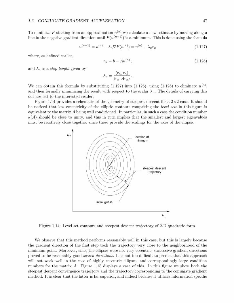
1.6. CONJUGATE GRADIENT ACCELERATION 47
To minimize F starting from an approximation u(n) we calculate a new estimate by moving along aline in the negative gradient direction until F (u(n+1)) is a minimum. This is done using the formula
u(n+1) = u(n) − λn∇F (u(n)) = u(n) + λnrn (1.127)
where, as defined earlier,rn = b − Au(n) , (1.128)
and λn is a step length given by
λn =〈rn, rn〉〈rn, Arn〉
.
We can obtain this formula by substituting (1.127) into (1.126), using (1.128) to eliminate u(n),and then formally minimizing the result with respect to the scalar λn. The details of carrying thisout are left to the interested reader.
Figure 1.14 provides a schematic of the geometry of steepest descent for a 2×2 case. It shouldbe noticed that low eccentricity of the elliptic contours comprising the level sets in this figure isequivalent to the matrix A being well conditioned. In particular, in such a case the condition numberκ(A) should be close to unity, and this in turn implies that the smallest and largest eigenvaluesmust be relatively close together since these provide the scalings for the axes of the ellipse.
initial guess
location of minimum
steepest descent trajectory
u1
u2
Figure 1.14: Level set contours and steepest descent trajectory of 2-D quadratic form.
We observe that this method performs reasonably well in this case, but this is largely becausethe gradient direction of the first step took the trajectory very close to the neighborhood of theminimum point. Moreover, since the ellipses were not very eccentric, successive gradient directionsproved to be reasonably good search directions. It is not too difficult to predict that this approachwill not work well in the case of highly eccentric ellipses, and correspondingly large conditionnumbers for the matrix A. Figure 1.15 displays a case of this. In this figure we show both thesteepest descent convergence trajectory and the trajectory corresponding to the conjugate gradientmethod. It is clear that the latter is far superior, and indeed because it utilizes information specific
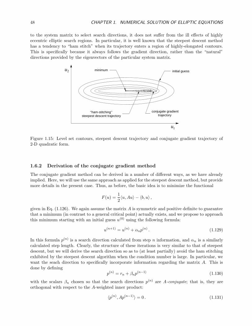
48 CHAPTER 1. NUMERICAL SOLUTION OF ELLIPTIC EQUATIONS
to the system matrix to select search directions, it does not suffer from the ill effects of highlyeccentric elliptic search regions. In particular, it is well known that the steepest descent methodhas a tendency to “ham stitch” when its trajectory enters a region of highly-elongated contours.This is specifically because it always follows the gradient direction, rather than the “natural”directions provided by the eigenvectors of the particular system matrix.
initial guessminimum
conjugate gradient trajectory
‘‘ham-stitching’’ steepest descent trajectory
u1
u2
Figure 1.15: Level set contours, steepest descent trajectory and conjugate gradient trajectory of2-D quadratic form.
1.6.2 Derivation of the conjugate gradient method
The conjugate gradient method can be derived in a number of different ways, as we have alreadyimplied. Here, we will use the same approach as applied for the steepest descent method, but providemore details in the present case. Thus, as before, the basic idea is to minimize the functional
F (u) =1
2〈u,Au〉 − 〈b, u〉 ,
given in Eq. (1.126). We again assume the matrix A is symmetric and positive definite to guaranteethat a minimum (in contrast to a general critical point) actually exists, and we propose to approachthis minimum starting with an initial guess u(0) using the following formula:
u(n+1) = u(n) + αnp(n) . (1.129)
In this formula p(n) is a search direction calculated from step n information, and αn is a similarlycalculated step length. Clearly, the structure of these iterations is very similar to that of steepestdescent, but we will derive the search direction so as to (at least partially) avoid the ham stitchingexhibited by the steepest descent algorithm when the condition number is large. In particular, wewant the seach direction to specifically incorporate information regarding the matrix A. This isdone by defining
p(n) = rn + βnp(n−1) (1.130)
with the scalars βn chosen so that the search directions p(n) are A-conjugate; that is, they areorthogonal with respect to the A-weighted inner product:
〈p(n), Ap(n−1)〉 = 0 . (1.131)
1.6. CONJUGATE GRADIENT ACCELERATION 49
Using (1.130) in this expression yields
〈rn, Ap(n−1)〉 + βn〈p(n−1), Ap(n−1)〉 = 0 ,
or
βn = − 〈rn, Ap(n−1)〉〈p(n−1), Ap(n−1)〉 . (1.132)
We observe that the form of the denominator in this expression requires positive definiteness of Ato guarantee existence of βn.
There are at least two different (but equivalent) ways to determine the αns. One is to requirethat successive residuals always be orthogonal (in the usual inner product), and the other is todirectly minimize F (u) with respect to αn. The first of these is trivial; we will apply the secondbecause this will at the same time provide some of the missing details of deriving the steepestdescent formula. Thus, we substitute Eq. (1.129) into Eq. (1.126) to obtain
F (u(n+1)) =1
2〈(u(n) + αnp(n)), A(u(n) + αnp(n))〉 − 〈b, (u(n) + αnp(n))〉
=1
2
[〈u(n), Au(n)〉 + αn〈p(n), Au(n)〉 + αn〈u(n), Ap(n)〉 + α2
n〈p(n), Ap(n)〉]
−〈b, u(n)〉 − αn〈b, p(n)〉 .
To minimize this expression with respect to αn we set
∂F (u(n+1))
∂αn= 0 ,
which leads to
1
2
[〈p(n), Au(n)〉 + 〈u(n), Ap(n)〉 + 2αn〈p(n), Ap(n)〉
]= 〈b, p(n)〉 .
But since A is symmetric this can be simplified to
〈p(n), Au(n)〉 + αn〈p(n), Ap(n)〉 = 〈b, p(n)〉 .
Now recall that Au(n) = b − rn to express the above as
αn =〈p(n), rn〉
〈p(n), Ap(n)〉 . (1.133)
The preceding formulas can be cast in a slightly different form, as shown by Saad [5]. Inparticular, from (1.129) and the form of the basic linear system being solved, it can be shown thatthe residual can be calculated from the recursion
rn+1 = rn − αnAp(n)
as an alternative to directly calculating it from the definition. Then, with this formula we can userequired orthogonality of the residuals to write
〈rn − αnAp(n), rn〉 = 0 ,
from which follows an alternative formula for αn:
αn =〈rn, rn〉
〈Ap(n), rn〉. (1.134)

50 CHAPTER 1. NUMERICAL SOLUTION OF ELLIPTIC EQUATIONS
Via analogous manipulations one can also obtain a simplified formula for βn:
βn =〈rn+1, rn+1〉〈rn, rn〉
. (1.135)
It is indicated in Hageman and Young [11] that these formulations are equivalent and are obtainedfrom the following identities proven in Hestenes and Stiefel [26]:
〈rn, rm〉 = 0 ∀ m 6= n
〈p(n), Ap(m)〉 = 0 ∀ m 6= n
〈rn, Ap(m)〉 = 0 ∀ m 6= n and m 6= n + 1 .
We can now provide a pseudo-language algorithm corresponding to the preceding equations, inthis case following the presentation in [11].
Algorithm 1.3 (CG method) Compute r0 = b − Au(0) and set p(0) = r0. Then carry out thefollowing steps:
Do n = 0,maxit
1. Calculate step length αn
αn = 〈p(n), rn〉/〈p(n), Ap(n)〉
2. Update solution valuesu(n+1) = u(n) + αnp(n)
3. Calculate residual based on updated solution
rn+1 = b − Au(n+1)
If residual is sufficiently small, stop
4. Calculate conjugate direction for next iteration
βn+1 = −〈rn+1, Ap(n)〉/〈p(n), Ap(n)〉 ,
p(n+1) = rn+1 + βn+1p(n)
Repeat j
1.6.3 Relationship of CG to other methods
We hinted in the opening paragraph of this section that there are relationships between the con-jugate gradient method and other widely-studied approaches for solving sparse linear systems. Inthis section we will briefly consider these. The first is Chebyshev acceleration, which is a so-calledpolynomial acceleration method that has been thoroughly studied. From its relation to the CGmethod we will be able to deduce the convergence rate of CG iterations. The second related classof methods is that associated with use of Krylov subspaces. These are also formally equivalent topolynomial accelerations, and thus also to the CG method. One of the currently most often usedof such methods is GMRES.
Chebyshev acceleration is often proposed as a method for accelerating other iterative proceduresbecause it is able to make use of more information than that simply from the most recent iterate.Indeed, the Chebyshev polynomials satisfy a three term recursion relation leading to a natural

1.7. INTRODUCTION TO MULTIGRID PROCEDURES 51
acceleration technique involving two iteration levels to produce a third. It turns out that the CGmethod can be recast into this form (see e.g., [5], [11] or [13]). We will not provide the details heresince we do not plan to develop this further in these lectures, but an important aspect of this isthat if bounds for the eigenvalues of the corresponding iteration matrix are known, the convergencerate can be predicted. In any case, this leads to the following result:
‖en‖A ≤ 2
[√κ − 1√κ + 1
]n
‖e0‖A , (1.136)
where en is the exact error defined earlier in (1.14), ‖ · ‖A is the norm induced by the A-weightedinner product, and κ is the condition number of the system matrix. It should be observed thatthe form of Eq. (1.136) is no different from that of any other linearly convergent procedure; onthe other hand, it depends only on the square root of the condition number, rather than on thecondition number, itself, as is often the case.
To demonstrate the connection of conjugate gradient methods to those based on use of Krylovsubspaces, we first remind the reader how a Krylov subspace is defined. As usual we considerthe system of equations Au = b to be solved iteratively starting with an initial guess u(0) andcorresponding residual r0. We then construct the sequence of vectors r0, Ar0, A
2r0, . . . , Am−1r0
and define the Krylov subspace u0 + Km by
Km(A, r0) = spanr0, Ar0, A2r0, . . . , A
m−1r0 . (1.137)
It is assumed that this set of vectors can be used to approximate the basis needed to construct thesolution u to the system whose matrix is A. Thus,
u = c0r0 + c1Ar0 + c2A2r0 + · · · + cm−1A
m−1r0 .
This represents a polynomial acceleration method of the sort we have already discussed in thecontext of Chebyshev acceleration, and it shows that all three of conjugate gradient, Chebyshevand Krylov subspace methods are related.
1.7 Introduction to Multigrid Procedures
In this section we will introduce one of the most important modern approaches to solving sparselinear systems arising from discretization of elliptic PDEs, viz., multigrid methods. We will beginwith a somewhat general overview of the procedure, and follow this with details of the two-gridmethod and finally the additional developments needed for full multigrid.
1.7.1 Some basic ideas
The basic notions underlying construction of multigrid (MG) methods have been known for a verylong time; they are the following:
i) use of relaxation-type methods as smoothing operators on fine grids;
ii) recursive application of coarse-grid (defect) corrections, and
iii) nested iteration.
52 CHAPTER 1. NUMERICAL SOLUTION OF ELLIPTIC EQUATIONS
Items i) and iii) have been used together for a wide range of problems over a long period of time,and it turns out that this is the last step in what is now known as the full multigrid (FMG) procedure.The first application of i) and ii) together is apparently due to Fedorenko [27] in 1961. In 1966Bachvalov [28] suggested combining this with iii), but he did not actually implement the scheme.It is the proper combination of all three elements that leads to the extremely good theoreticalconvergence rates for multigrid methods, as demonstrated by Brandt [29], and by Bramble et al.[30].
Of all sparse matrix techniques, only the various multigrid and domain decomposition proce-dures exhibit convergence rates that approach being independent of grid spacing h (i.e., independentof the number of equations in the system). Moreover, multigrid methods can be constructed sothat the total arithmetic required to solve a system of N equations is only O(N). Hence, as a class,these methods are optimal.
It is important to observe that convergence rate independent of h is not, alone, sufficient toguarantee efficiency. In particular, direct elimination methods require only a single “iteration,”independent of h, to obtain the exact (to machine precision) solution. But we are well awarethat such methods cannot be readily applied to large sparse systems because each such “iteration”requires O(N 3) arithmetic operations.
In this introduction we will closely follow the treatment of Stuben and Trottenberg [31] (notethat this same approach can also be found in the more recent monograph by Briggs [32]), presentingfirst a fairly detailed discussion of the two-grid case, and then a few aspects of the `-grid methods,followed by a brief discussion of the full multigrid procedure.
We begin by developing the notions corresponding to i) and ii) above. It is interesting to notethat this is analogous to use of deferred corrections or in the context of linear systems as treatedhere, iterative improvement (see Bohmer and Stetter [33] for further discussions). In particular,suppose we approximately solve the system
Ahuh = bh , (1.138)
and obtain the iterate u(n)h . We comment that while the algorithms of previous sections did not
specifically make use of the fact that the sparse systems to which they were applied arose bydiscretizing a PDE, our presentation of MG methods does reflect this. In particular, the h subscriptsappearing in the above equation indicate that this system is a discrete approximation formulatedwith a grid of spacing h.
Now observe that if we could calculate the exact error e(n)h by some means, we could add this
to u(n)h to obtain the exact solution (to within machine precision); i.e., we have
uh = u(n)h + e
(n)h .
To obtain an equation for e(n)h we rearrange this as
e(n)h = uh − u
(n)h ,
and multiplication by Ah yields
Ahe(n)h = Ahuh − Ahu
(n)h = bh − Ahu
(n)h = r
(n)h .
Hence,
Ahe(n)h = r
(n)h . (1.139)
1.7. INTRODUCTION TO MULTIGRID PROCEDURES 53
This is usually called the defect equation.
An important observation is that if e(n)h is smooth, it is not necessary to determine it exactly
in order to obtain a significant improvement in the accuracy of u(n)h . Namely, we could solve the
defect equation on a coarser grid, say of spacing 2h, and still obtain a useful improvement in the
solution u(n)h . In particular, we might solve
A2he(n)2h = r
(n)2h . (1.140)
and then form
u(n+1)h = u
(n)h + e
(n)2h . (1.141)
Equation (1.140) can be solved much more easily than can (1.139) because the solution vectorwill contain approximately a factor of four fewer components (for a 2-D problem). On the otherhand, if 2h is the coarsest grid employed (as will be the case in the next section), then Eq. (1.140)must be solved “exactly” in the sense that iteration errors should be smaller than the minimum ofthe required iteration tolerance and truncation errors on the finest (i.e., h-) grid in order to avoidintroduction of additional error.
It is clear from (1.140) and (1.141) that there are incompatibilities in vector lengths. For
example, since e(n)2h is roughly four times shorter than r
(n)h the latter must be appropriately shortened
by applying what is termed a restriction operator. If we let Sh denote the set of points in the gridof spacing h and similarly let S2h denote those of the 2h-grid, in general it will be true thatSh ∩ S2h 6= ∅. Thus, we could (and sometimes do) define the restriction operator so as to merelypick out the points lying in this intersection (this is termed injection). However, for theoreticalreasons we will discuss in more detail later, this is not always done. We will consider a morewidely-used restriction operator below.
It is also easy to see that e(n)2h is too short for use in Eq. (1.141) by a factor of about four.
This is remedied by using a prolongation operator, which merely amounts to interpolation betweenthe S2h and Sh point sets. As with restriction, there are many alternatives for constructing theprolongation operator, and we shall treat this in more detail later.
By this time we have accumulated enough information to make a first attempt at constructinga basic multigrid algorithm. This will be the topic of the next section.
1.7.2 The h-2h two-grid algorithm
In this subsection we will first present a formal algorithm corresponding to the two-grid h-2hmultigrid method. We will follow this with a fairly detailed discussion of each of the main steps ofthe procedure, and we will then derive the general fixed-point form of this method.
Algorithm 1.4 (Two-grid MG) Suppose n iterations have been completed. Compute the n+1th
iterate by carrying out the following steps.
1. Obtain an approximate solution u(n+1)∗
h to Ahuh = bh using a relaxation-like method to ac-
complish fine-grid smoothing starting from the (current) “initial guess” u(n)h , and compute the
residual,
r(n+1)h = bh − Ahu(n+1)∗
2. Test convergence: if ‖r(n+1)h ‖ < ε, then stop; else continue to step 3.
54 CHAPTER 1. NUMERICAL SOLUTION OF ELLIPTIC EQUATIONS
3. Restrict residual to coarse grid (fine-to-coarse grid transfer)
r(n+1)2h = R2h
h r(n+1)h
4. “Exactly” solve the defect equation
A2he(n+1)2h = r
(n+1)2h
5. Prolongate (interpolate) correction e(n+1)2h (coarse-to-fine grid transfer)
e(n+1)h = Ph
2he(n+1)2h
6. Compute new approximation to uh,
u(n+1)h = u
(n+1)∗
h + e(n+1)h
and go to 1.
It is important to consider each step of this algorithm in some detail; we do this in the followingsubsections.
Fine-grid smoothing
The first step requires computation of an approxinate solution on the finest grid. But the un-derlying philosophy in carrying this out is now considerably different than would be the case in asingle-grid algorithm. In particular, it is not necessary to obtain an extremely accurate approxi-mation as would normally be the case. We can argue this heuristically by noting that the residualcarried to the coarser grid, and hence the defect correction, depends (linearly) on the error in theapproximate solution. Thus, we would expect (correctly) that the defect correction should, to someextent, automatically compensate for errors in the fine-grid approximation of uh (the larger theerror, the larger the defect correction). But we must keep in mind one of our basic assumptions that
permits use of a defect correction computed on a coarser grid: e(n+1)2h is presumed to be smooth.
To guarantee this, it must be true that r(n+1)h (or, at least r
(n+1)2h ) is smooth, and this implies that
enough iterations must be performed on the fine grid to eliminate the high-wavenumber contribu-
tions to the error. These correspond to lack of smoothness in u(n+1)∗
h . At the same time, we shouldnot perform significantly more iterations than are required to accomplish this.
These ideas imply that the iteration method employed on the fine grid need not be rapidlyconvergent in the sense that its spectral radius is very much less than unity, but rather thatthe method should possess strong smoothing properties with respect to high wavenumbers. It isinteresting to note that this is precisely the behavior of the typical relaxation schemes such asJacobi and Gauss-Seidel (but not optimal SOR) iterations. All of these efficiently remove high-wavenumber errors but are very inefficient at reducing the low-wavenumber errors. (Recall thatthe spectral radius of the Jacobi iteration matrix is set by the lowest possible wavenumbers.)
In connection with these notions we can observe that the underlying reason for the effectivenessof MG procedures is that they do not attempt to eliminate low-wavenumber error during the fine-grid calculations. Rather, they carry out low-wavenumber error reduction on coarse grids wherethe low wavenumbers become “high” wavenumbers with respect to that particular grid, and arethus more easily removed.
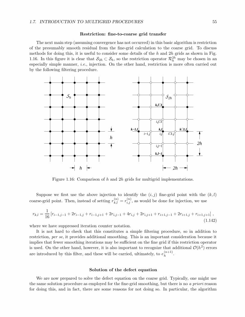
1.7. INTRODUCTION TO MULTIGRID PROCEDURES 55
Restriction: fine-to-coarse grid transfer
The next main step (assuming convergence has not occurred) in this basic algorithm is restrictionof the presumably smooth residual from the fine-grid calculation to the coarse grid. To discussmethods for doing this, it is useful to consider some details of the h and 2h grids as shown in Fig.1.16. In this figure it is clear that S2h ⊂ Sh, so the restriction operator R2h
h may be chosen in anespecially simple manner, i.e., injection. On the other hand, restriction is more often carried outby the following filtering procedure.
h
h
2h
2h
Sh S2h
i,j i+1,ji−1,j
i,j−1
i,j+1
k,l
k,l+1
k,l−1
k−1,l k+1,l
Figure 1.16: Comparison of h and 2h grids for multigrid implementations.
Suppose we first use the above injection to identify the (i, j) fine-grid point with the (k, l)
coarse-grid point. Then, instead of setting r(n)k,l = r
(n)i,j , as would be done for injection, we use
rk,l =1
16[ri−1,j−1 + 2ri−1,j + ri−1,j+1 + 2ri,j−1 + 4ri,j + 2ri,j+1 + ri+1,j−1 + 2ri+1,j + ri+1,j+1] ,
(1.142)where we have suppressed iteration counter notation.
It is not hard to check that this constitutes a simple filtering procedure, so in addition torestriction, per se, it provides additional smoothing. This is an important consideration because itimplies that fewer smoothing iterations may be sufficient on the fine grid if this restriction operatoris used. On the other hand, however, it is also important to recognize that additional O(h2) errors
are introduced by this filter, and these will be carried, ultimately, to e(n+1)h .
Solution of the defect equation
We are now prepared to solve the defect equation on the coarse grid. Typically, one might usethe same solution procedure as employed for the fine-grid smoothing, but there is no a priori reasonfor doing this, and in fact, there are some reasons for not doing so. In particular, the algorithm
56 CHAPTER 1. NUMERICAL SOLUTION OF ELLIPTIC EQUATIONS
employed for fine-grid smoothing need not be rapidly convergent, whereas it is important that theprocedure used for solving the defect equation be quite efficient since an exact solution to thisequation is required.
Prolongation: coarse-to-fine grid transfer
Just as there are many possibilities for restriction operators, there are also many ways in whichprolongation (interpolation) may be done (and as we will note later, these are closely related torestriction). Clearly, the details of prolongation will depend on the specific type of h-2h griddingused. In particular, Fig. 1.16 is not the only possibility; the interested reader may want to consultHackbusch [34] for more details on this and other aspects of multigrid methods in general. For thegrid configuration depicted above, linear interpolation described in the following algorithm is oftenused.Algorithm 1.5 (Prolongation: coarse-to-fine grid transfer of defect correction) After “ex-act” solution of defect equation, perform the following steps to interpolate results to fine grid.
1. Interpolate along horizontal lines to obtain
e(n+1)i+1,j =
1
2
(e(n+1)k,l + e
(n+1)k+1,l
)
2. Interpolate along vertical lines to obtain
e(n+1)i,j+1 =
1
2
(e(n+1)k,l + e
(n+1)k,l+1
)
3. Obtain results for interior points not appearing on the 2h-grid lines by averaging the fournearest corner neighbors:
e(n+1)i−1,j−1 =
1
4
(e(n+1)k−1,l−1 + e
(n+1)k−1,l + e
(n+1)k,l−1 + e
(n+1)k,l
)
We can now complete the current multigrid iteration by calculating
u(n+1)h = u
(n+1)∗
h + e(n+1)h . (1.143)
But it is important to note at this point that new high-wavenumber errors will have been introducedby the interpolation process, and these must be removed. This is done with a final smoothing onthe fine grid, to be performed before convergence is tested. Recall that in the h-2h algorithm, wetested convergence after an initial fine-grid smoothing operation, but in fact in this case the finalsmoothing discussed here and the initial one of the algorithm are actually the same if more thanone overall iteration is to be performed.
Fixed-point form of 2-grid multigrid procedures
It is interesting to note at this point that the above algorithm can be cast in the standard formof a linear fixed-point iteration. This can be done via the following steps. First, recall that
r(n+1)h = bh − Ahu
(n+1)∗
h ,
and thusr(n+1)2h = R2h
h
(bh − Ahu
(n+1)∗
h
).
1.7. INTRODUCTION TO MULTIGRID PROCEDURES 57
Now the formal solution to the defect equation is
e(n+1)2h = A−1
2h r(n+1)2h
= A−12h R2h
h
(b − Ahu
(n+1)∗
h
),
so it follows thate(n+1)h = Ph
2hA−12h R2h
h
(bh − Ahu
(n+1)∗
h
).
Thus, it follows that
u(n+1)h = u
(n+1)∗
h + e(n+1)h
= u(n+1)∗
h + Ph2hA−1
2h R2hh
(bh − Ahu
(n+1)∗
h
)
=(I −Ph
2hA−12h R2h
h Ah
)u
(n+1)∗
h + Ph2hA−1
2h R2hh bh .
Next recall that u(n+1)∗
h results from some number ν of smoothing operations which we willassume correspond to a linear fixed-point iteration written as
u(m+1)h = Su
(m)h + k ,
where S is a smoothing operator, e.g., Gauss-Seidel iteration, and m = 0, 1, . . . , ν, with m = 0
corresponding to u(n)h . It is easily shown that
u(n+1)∗
h = Sνu(n)h +
(I + S + · · · + Sν−1
)k
= Sνu(n)h +
(I +
ν−1∑
m=1
Sm
)k .
Next substitute these results into the above expression for u(n+1)h to obtain
u(n+1)h =
(I −Ph
2hA−12h R2h
h Ah
)[Sνu
(n)h +
(I +
ν−1∑
m=1
Sm
)k
]+ Ph
2hA−12h R2h
h bh .
Now associated with S there is a splitting matrix, say Q, such that
k = Q−1bh ,
so the above becomes
u(n+1)h =
(I −Ph
2hA−12h R2h
h Ah
)[Sνu
(n)h +
(I +
ν−1∑
m=1
Sm
)Q−1bh
]+ Ph
2hA−12h R2h
h bh
=(I −Ph
2hA−12h R2h
h Ah
)Sνu
(n)h
+
[(I −Ph
2hA−12h R2h
h Ah
)(I +
ν−1∑
m=1
Sm
)Q−1 + Ph
2hA−12h R2h
h
]bh . (1.144)
Clearly, this is in the usual linear fixed-point form with
G ≡(I −Ph
2hA−12h R2h
h Ah
)Sν ,
k ≡[(
I −Ph2hA−1
2h R2hh Ah
)(I +
ν−1∑
m=1
Sm
)Q−1 + Ph
2hA−12h R2h
h
]bh .
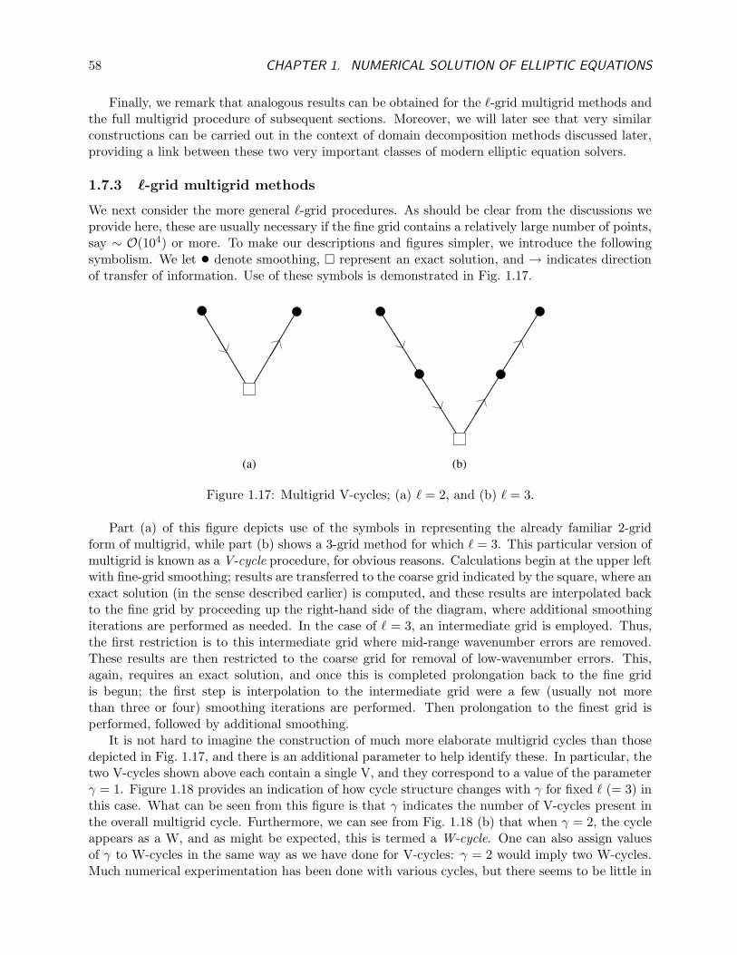
58 CHAPTER 1. NUMERICAL SOLUTION OF ELLIPTIC EQUATIONS
Finally, we remark that analogous results can be obtained for the `-grid multigrid methods andthe full multigrid procedure of subsequent sections. Moreover, we will later see that very similarconstructions can be carried out in the context of domain decomposition methods discussed later,providing a link between these two very important classes of modern elliptic equation solvers.
1.7.3 `-grid multigrid methods
We next consider the more general `-grid procedures. As should be clear from the discussions weprovide here, these are usually necessary if the fine grid contains a relatively large number of points,say ∼ O(104) or more. To make our descriptions and figures simpler, we introduce the followingsymbolism. We let • denote smoothing, represent an exact solution, and → indicates directionof transfer of information. Use of these symbols is demonstrated in Fig. 1.17.
(a) (b)
Figure 1.17: Multigrid V-cycles; (a) ` = 2, and (b) ` = 3.
Part (a) of this figure depicts use of the symbols in representing the already familiar 2-gridform of multigrid, while part (b) shows a 3-grid method for which ` = 3. This particular version ofmultigrid is known as a V-cycle procedure, for obvious reasons. Calculations begin at the upper leftwith fine-grid smoothing; results are transferred to the coarse grid indicated by the square, where anexact solution (in the sense described earlier) is computed, and these results are interpolated backto the fine grid by proceeding up the right-hand side of the diagram, where additional smoothingiterations are performed as needed. In the case of ` = 3, an intermediate grid is employed. Thus,the first restriction is to this intermediate grid where mid-range wavenumber errors are removed.These results are then restricted to the coarse grid for removal of low-wavenumber errors. This,again, requires an exact solution, and once this is completed prolongation back to the fine gridis begun; the first step is interpolation to the intermediate grid were a few (usually not morethan three or four) smoothing iterations are performed. Then prolongation to the finest grid isperformed, followed by additional smoothing.
It is not hard to imagine the construction of much more elaborate multigrid cycles than thosedepicted in Fig. 1.17, and there is an additional parameter to help identify these. In particular, thetwo V-cycles shown above each contain a single V, and they correspond to a value of the parameterγ = 1. Figure 1.18 provides an indication of how cycle structure changes with γ for fixed ` (= 3) inthis case. What can be seen from this figure is that γ indicates the number of V-cycles present inthe overall multigrid cycle. Furthermore, we can see from Fig. 1.18 (b) that when γ = 2, the cycleappears as a W, and as might be expected, this is termed a W-cycle. One can also assign valuesof γ to W-cycles in the same way as we have done for V-cycles: γ = 2 would imply two W-cycles.Much numerical experimentation has been done with various cycles, but there seems to be little in
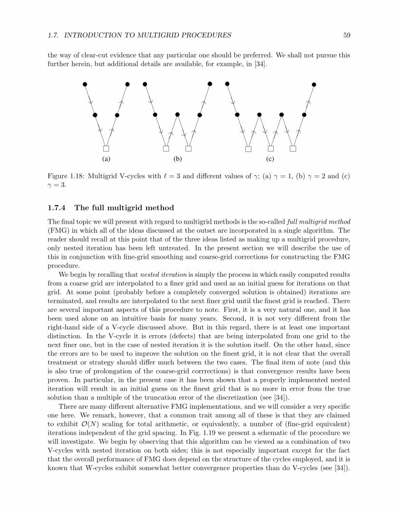
1.7. INTRODUCTION TO MULTIGRID PROCEDURES 59
the way of clear-cut evidence that any particular one should be preferred. We shall not pursue thisfurther herein, but additional details are available, for example, in [34].
(a) (b) (c)
Figure 1.18: Multigrid V-cycles with ` = 3 and different values of γ; (a) γ = 1, (b) γ = 2 and (c)γ = 3.
1.7.4 The full multigrid method
The final topic we will present with regard to multigrid methods is the so-called full multigrid method(FMG) in which all of the ideas discussed at the outset are incorporated in a single algorithm. Thereader should recall at this point that of the three ideas listed as making up a multigrid procedure,only nested iteration has been left untreated. In the present section we will describe the use ofthis in conjunction with fine-grid smoothing and coarse-grid corrections for constructing the FMGprocedure.
We begin by recalling that nested iteration is simply the process in which easily computed resultsfrom a coarse grid are interpolated to a finer grid and used as an initial guess for iterations on thatgrid. At some point (probably before a completely converged solution is obtained) iterations areterminated, and results are interpolated to the next finer grid until the finest grid is reached. Thereare several important aspects of this procedure to note. First, it is a very natural one, and it hasbeen used alone on an intuitive basis for many years. Second, it is not very different from theright-hand side of a V-cycle discussed above. But in this regard, there is at least one importantdistinction. In the V-cycle it is errors (defects) that are being interpolated from one grid to thenext finer one, but in the case of nested iteration it is the solution itself. On the other hand, sincethe errors are to be used to improve the solution on the finest grid, it is not clear that the overalltreatment or strategy should differ much between the two cases. The final item of note (and thisis also true of prolongation of the coarse-grid corrrections) is that convergence results have beenproven. In particular, in the present case it has been shown that a properly implemented nestediteration will result in an initial guess on the finest grid that is no more in error from the truesolution than a multiple of the truncation error of the discretization (see [34]).
There are many different alternative FMG implementations, and we will consider a very specificone here. We remark, however, that a common trait among all of these is that they are claimedto exhibit O(N) scaling for total arithmetic, or equivalently, a number of (fine-grid equivalent)iterations independent of the grid spacing. In Fig. 1.19 we present a schematic of the procedure wewill investigate. We begin by observing that this algorithm can be viewed as a combination of twoV-cycles with nested iteration on both sides; this is not especially important except for the factthat the overall performance of FMG does depend on the structure of the cycles employed, and it isknown that W-cycles exhibit somewhat better convergence properties than do V-cycles (see [34]).

60 CHAPTER 1. NUMERICAL SOLUTION OF ELLIPTIC EQUATIONS
nested iteration
V-cycle
V-cycle
h
2h
4h
8h
= 2
= 3
Figure 1.19: Four-Level, V-cycle full multigrid schematic.
On the other hand, the computational work required in a W-cycle exceeds that of a V-cycle by asignificant amount, so we will analyze the simple V-cycles here. It is also important to note thatthe choice of a four-level scheme is simply to provide a non-trivial example, and as we will indicatein the sequel, larger numbers of levels may be necessary in some cases.
We now describe the manner in which an algorithm corresponding to this schematic would beexecuted, and we follow this with an analysis of the required total arithmetic. Figure 1.19 indicatesthat calculations begin with an exact solution on the coarsest (8h-) grid (recall our definition ofexact). This solution is then prolongated to the 4h-grid via interpolation. In this particular case, theprocess corresponds to nested iteration because it is the solution, itself, that is prolongated, and notthe error. Then a small number of iterations is performed on the 4h-grid to accomplish smoothing,and the residual is then restricted to the 8h-grid for further removal of low-wavenumber errors.Because this is the coarsest grid, the exact solution must be found for the defect equation. Thenext step is to prolongate this error back to the 4h-grid where it is used to update the solution. Atthis point a few smoothing iterations (usually only one) may be applied before the nested iterationstep is invoked to transfer the solution from the 4h-grid to the 2h-grid. Once this transfer is made,smoothing iterations are again applied before restriction of the residual back to the 4h-grid. Then,some additional smoothing may be done before restriction back to the 8h-grid. Next, the exacterror is computed one more time, and prolongated back to the 4h-grid where it is combined withthe solution obtained by injection from the 2h-grid. Nested iteration of the solution is now appliedsuccessively between the 4h- and 2h-grids, and then after smoothing on the 2h-grid, one more timebetween the 2h- and h-grids.
As noted above, the solution on the fine h-grid thus obtained can be shown to be within anO(1) constant of the converged solution on the fine grid. Thus, it should be expected that afew additional smoothing iterations should be sufficient to complete the solution, obtained fromonly a single pass through the FMG algorithm. In practice, however, this is not always the case.If the desired tolerance has not been met, it is common practice to employ several additional V-cycles. We will, in what follows, assume that a single pass through the FMG procedure is sufficient;modifications needed to account for other situations are not difficult, and they, in general, will notstrongly influence the conclusions we will draw.
It will be convenient to refer to the (2-D) h-grid as the N -point grid, the 2h-grid as the N/4-point grid, etc. We will first estimate the number of arithmetic operations required for exact solves
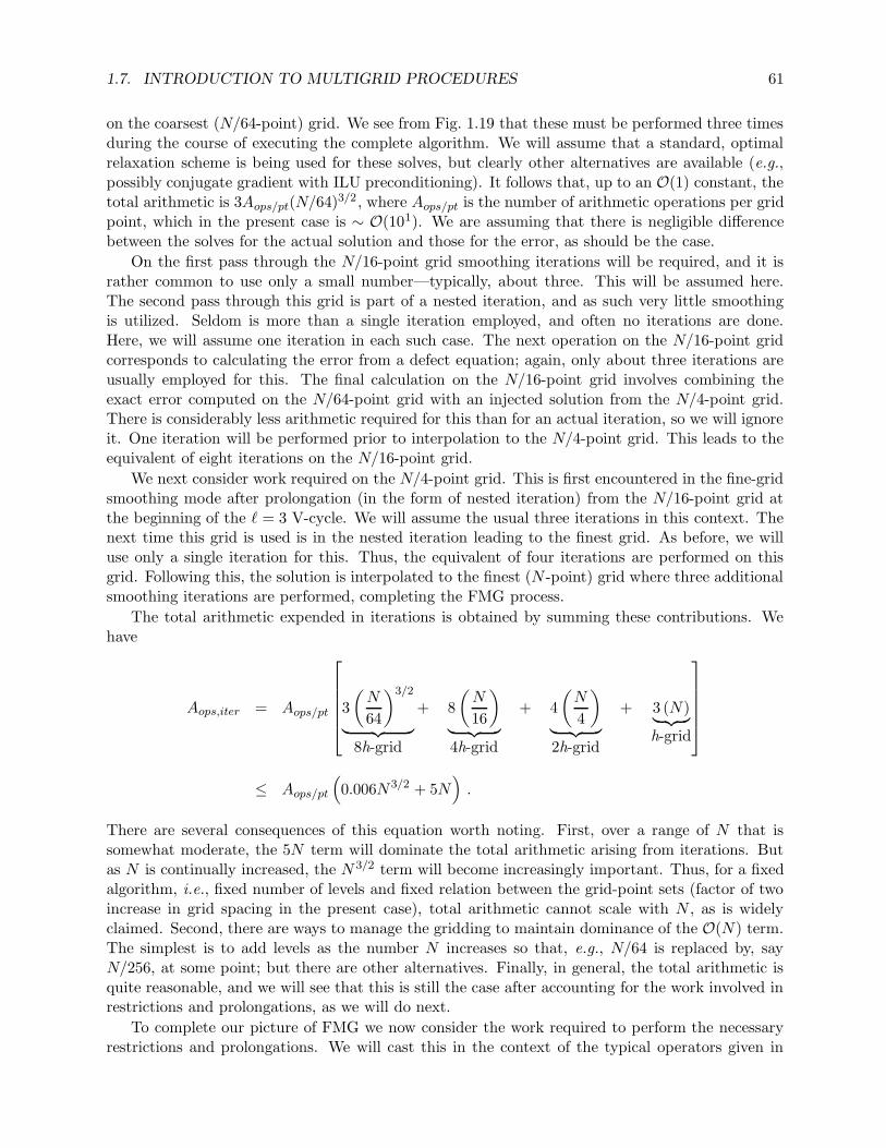
1.7. INTRODUCTION TO MULTIGRID PROCEDURES 61
on the coarsest (N/64-point) grid. We see from Fig. 1.19 that these must be performed three timesduring the course of executing the complete algorithm. We will assume that a standard, optimalrelaxation scheme is being used for these solves, but clearly other alternatives are available (e.g.,possibly conjugate gradient with ILU preconditioning). It follows that, up to an O(1) constant, thetotal arithmetic is 3Aops/pt(N/64)3/2 , where Aops/pt is the number of arithmetic operations per gridpoint, which in the present case is ∼ O(101). We are assuming that there is negligible differencebetween the solves for the actual solution and those for the error, as should be the case.
On the first pass through the N/16-point grid smoothing iterations will be required, and it israther common to use only a small number—typically, about three. This will be assumed here.The second pass through this grid is part of a nested iteration, and as such very little smoothingis utilized. Seldom is more than a single iteration employed, and often no iterations are done.Here, we will assume one iteration in each such case. The next operation on the N/16-point gridcorresponds to calculating the error from a defect equation; again, only about three iterations areusually employed for this. The final calculation on the N/16-point grid involves combining theexact error computed on the N/64-point grid with an injected solution from the N/4-point grid.There is considerably less arithmetic required for this than for an actual iteration, so we will ignoreit. One iteration will be performed prior to interpolation to the N/4-point grid. This leads to theequivalent of eight iterations on the N/16-point grid.
We next consider work required on the N/4-point grid. This is first encountered in the fine-gridsmoothing mode after prolongation (in the form of nested iteration) from the N/16-point grid atthe beginning of the ` = 3 V-cycle. We will assume the usual three iterations in this context. Thenext time this grid is used is in the nested iteration leading to the finest grid. As before, we willuse only a single iteration for this. Thus, the equivalent of four iterations are performed on thisgrid. Following this, the solution is interpolated to the finest (N -point) grid where three additionalsmoothing iterations are performed, completing the FMG process.
The total arithmetic expended in iterations is obtained by summing these contributions. Wehave
Aops,iter = Aops/pt
3
(N
64
)3/2
︸ ︷︷ ︸8h-grid
+ 8
(N
16
)
︸ ︷︷ ︸4h-grid
+ 4
(N
4
)
︸ ︷︷ ︸2h-grid
+ 3 (N)︸ ︷︷ ︸h-grid
≤ Aops/pt
(0.006N 3/2 + 5N
).
There are several consequences of this equation worth noting. First, over a range of N that issomewhat moderate, the 5N term will dominate the total arithmetic arising from iterations. Butas N is continually increased, the N 3/2 term will become increasingly important. Thus, for a fixedalgorithm, i.e., fixed number of levels and fixed relation between the grid-point sets (factor of twoincrease in grid spacing in the present case), total arithmetic cannot scale with N , as is widelyclaimed. Second, there are ways to manage the gridding to maintain dominance of the O(N) term.The simplest is to add levels as the number N increases so that, e.g., N/64 is replaced by, sayN/256, at some point; but there are other alternatives. Finally, in general, the total arithmetic isquite reasonable, and we will see that this is still the case after accounting for the work involved inrestrictions and prolongations, as we will do next.
To complete our picture of FMG we now consider the work required to perform the necessaryrestrictions and prolongations. We will cast this in the context of the typical operators given in
62 CHAPTER 1. NUMERICAL SOLUTION OF ELLIPTIC EQUATIONS
Eq. (1.142) and Algorithm 1.5. In particular, it can be seen from (1.142) that the total arithmeticrequired for restriction is approximately 50% greater than that needed per point for a typical relax-ation iteration. At the same time, the linear interpolation formulas of the prolongation algorithmshow that this step requires somewhat less than 50% of an iteration per grid point. Furthermore, inthe FMG scheme of Fig. 1.19 the number of prolongations exceeds that of restrictions, so countingeach of these as one iteration will provide an upper bound for this auxiliary arithmetic.
From the figure it is easily seen that there are two restrictions to the N/64-point grid, and thusan equivalent of 2(N/64) units of work. There is one additional restriction to the N/16-point gridwith a corresponding N/16 units of work. There are three prolongations of the N/64-point gridresults, so this adds 3(N/16) work units, and there are two prolongations from the N/16-point gridto the N/4-point grid, giving 2(N/4) units of work. Finally, the prolongation from the N/4-pointgrid to the N -point grid gives an additional N units. Thus, the total arithmetic for restriction andprolongation is
Aops,r/p =
8h︷ ︸︸ ︷2
(N
64
)+
4h︷ ︸︸ ︷(N
16
)
︸ ︷︷ ︸restriction
+
4h︷ ︸︸ ︷3
(N
16
)+
2h︷ ︸︸ ︷2
(N
4
)+
h︷︸︸︷N
︸ ︷︷ ︸prolongation
< 2N ,
which implies that for the particular FMG form we are considering, all work associated withrestrictions and prolongations accounts for less than two iterations on the finest grid. Thus, thetotal arithmetic to complete one execution of the FMG algorithm depicted in Fig. 1.19 is
Atotal < Aops/pt
(0.006N 3/2 + 7N
). (1.145)
It is also of interest to compare this total arithmetic with that which would be required bya basic (optimal) relaxation method such as SOR on a grid of N points. Clearly, this would be∼ Aops/ptN
3/2, so it is easily seen that the speed up obtained from the multigrid formulation isquite considerable even if several FMG cycles are required.
1.7.5 Some concluding remarks
In this section we have provided a basic introduction to multigrid methods, but this has been,admittedly, rather cursory. There are many good references available from which the interestedreader can obtain much additional information (see [31], [32], [34] among many others). Here, wewill provide a few clarifying remarks, some of which can be found in the literature, and some ofwhich may not. We will first comment on MG convergence rate, which has been widely studied.In particular, as noted in [34], the convergence rate of 2-grid multigrid is, in fact, theoretically thesame as for full multigrid; viz., independent of discretization step size. But in practice this is notusually observed, and the 2-grid MG rate is sometimes quoted as O(N log N). One can readilysee from our analysis of total arithmetic that if only two grids are employed, unless there is anextreme difference in grid spacing between the fine and coarse grids, the coarse-grid (required)exact solutions will ultimately dominate the arithmetic, so the convergence rate will simply be therate associated with these solves, and this will not lead to O(N) arithmetic—and in most cases,not even O(N log N).
We next need to provide a comment concerning the relationship between restriction and pro-longation. We hinted earlier that these are related: in a somewhat loose sense they are inverses of
1.8. DOMAIN DECOMPOSITION METHODS 63
one another. There are analyses showing that for these two operations to work together properlyit is necessary that their matrix representations be transposes of one another. Hence, one mightfirst select an interpolation scheme for prolongation, and then construct its transposed matrix todetermine the restriction operator. But in practice this is often not done. For example, if injectionis used for restriction, no interpolation scheme employed for prolongation will have a matrix thatis the transpose of the injection matrix. This is one of the main arguments against employinginjection. In addition is the fact that typical restriction operators such as that given in Eq. (1.142)are actually low-pass filters. Hence, they provide additional smoothing of the fine-grid residual,permitting use of fewer iterations on the fine grid.
Finally, we must comment on the overall effectiveness of removing low-wavenumber error oncourse grids where it is best removed. In principle this seems like a perfectly reasonable notion. Butconsider the situation (often encountered, e.g. in CFD) wherein solution resolution on the finest gridis at best sufficient, and possibly not even that. We perform some smoothing iterations to estimatethis solution, and then we restrict to a yet coarser grid to remove low-wavenumber errors. Supposewe use the typical restriction operator of Eq. (1.142) to guarantee that the residuals transferred tothe coarse grid are smooth. Then on this coarse grid we solve the defect equation. Since results onthe fine grid are already barely resolved, the defect produced on the coarse grid will not be properlyresolve; it will be aliased, and the associated error will be interpolated back to the fine grid to beused as a “correction” to the solution. It is rather clear that such an approach has little chancefor success and, indeed, success of multigrid in problems where production of aliased solutions islikely has not been altogether satisfactory—O(N) arithmetic is essentially never observed. As aconsequence, we must be somewhat careful in our assessment of the performance capabilities ofmultigrid methods, and correspondingly in our choice of problems to which we attempt to applythem.
1.8 Domain Decomposition Methods
The basic ideas underlying domain decomposition were first proposed by Schwarz [35] in 1870 inthe context of constructing analytical solutions to elliptic PDEs on irregularly-shaped domains.Schwarz was able to prove convergence of an iterative procedure in which the domain is dividedinto two (or more) regularly-shaped, overlapping subdomains on which exact solutions could beconstructed, but on which some of the boundary conditions required by one subdomain must bedetermined from the solution in the other subdomain.
This approach was described by Mitchell and Griffiths [9], and earlier by Mitchell [36], to aidthe implementation of ADI methods on L-shaped domains, as depicted in Fig. 1.20. It is easilyseen from this figure that ADI-like procedures would be somewhat difficult to implement for thedomain, as a whole, but they are readily implemented on either Ω1 ∪ Ω3 or Ω2 ∪ Ω3. On the otherhand, a segment of the boundary (corresponding to the sets of filled grid points) is not specifiedfor each of these subdomains. However, if initially we guess the boundary values, say on Γ13, andsolve the PDE in Ω2 ∪Ω3, then we can use the computed result to provide the necessary boundaryvalues on Γ23 for the subdomain Ω1 ∪ Ω3. Then, the PDE can be solved in this region, in turnyielding a better estimate for boundary conditions on Γ13. This process is continued iterativelyuntil a desired level of convergence for the solution on the whole domain is achieved.
We can formally summarize this as follows for Dirichlet problems for Poisson’s equation,
−∆u = f(x, y) , (x, y) ∈ Ω(≡ Ω1 ∪ Ω2 ∪ Ω3) ,
u(x, y) = g(x, y) , (x, y) ∈ ∂Ω .
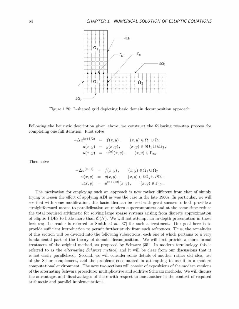
64 CHAPTER 1. NUMERICAL SOLUTION OF ELLIPTIC EQUATIONS
∂Ω3
∂Ω1
∂Ω2
Γ13Γ23
Ω1
Ω2Ω3
Figure 1.20: L-shaped grid depicting basic domain decomposition approach.
Following the heuristic description given above, we construct the following two-step process forcompleting one full iteration. First solve
−∆u(n+1/2) = f(x, y) , (x, y) ∈ Ω1 ∪ Ω3
u(x, y) = g(x, y) , (x, y) ∈ ∂Ω1 ∪ ∂Ω3 ,
u(x, y) = u(n)(x, y) , (x, y) ∈ Γ23 .
Then solve
−∆u(n+1) = f(x, y) , (x, y) ∈ Ω1 ∪ Ω2
u(x, y) = g(x, y) , (x, y) ∈ ∂Ω2 ∪ ∂Ω3 ,
u(x, y) = u(n+1/2)(x, y) , (x, y) ∈ Γ13 .
The motivation for employing such an approach is now rather different from that of simplytrying to lessen the effort of applying ADI as was the case in the late 1960s. In particular, we willsee that with some modification, this basic idea can be used with great success to both provide astraightforward means to parallelization on modern supercomputers and at the same time reducethe total required arithmetic for solving large sparse systems arising from discrete approximationof elliptic PDEs to little more than O(N). We will not attempt an in-depth presentation in theselectures; the reader is referred to Smith et al. [37] for such a treatment. Our goal here is toprovide sufficient introduction to permit further study from such references. Thus, the remainderof this section will be divided into the following subsections, each one of which pertains to a veryfundamental part of the theory of domain decomposition. We will first provide a more formaltreatment of the original method, as proposed by Schwarz [35]. In modern terminology this isreferred to as the alternating Schwarz method, and it will be clear from our discussions that itis not easily parallelized. Second, we will consider some details of another rather old idea, useof the Schur complement, and the problems encountered in attempting to use it in a moderncomputational environment. The next two sections will consist of expositions of the modern versionsof the alternating Schwarz procedure: multiplicative and additive Schwarz methods. We will discussthe advantages and disadvantages of these with respect to one another in the context of requiredarithmetic and parallel implementations.

1.8. DOMAIN DECOMPOSITION METHODS 65
Finally, we will briefly introduce the most recent development in domain decomposition andmultigrid methods, namely, the multi-level domain decomposition. This approach is quite possiblythe closest that one will be able to come in solving a wide range of elliptic problems in only O(N)arithmetic operations. It is worthwhile to recognize that these two approaches are, in a sense,complementary, and one would expect them to work well together. In particular, recall that thespectral radius of typical relaxation methods is usually similar in form to that of Jacobi iterations,given in Eq. (1.39) for Laplace-Dirichlet problems as the Taylor expansion
ρ(B) = 1 − 1
4
[(π
a
)2+(π
b
)2]
h2 + O(h4) ,
where a and b are lengths of the sides of a rectangular domain whose lower left-hand corner is atthe origin. It is important to note that there are two distinct ways in which this quantity can bemade small. First, we can make h large; this is the approach taken in multigrid methods whencarrying out coarse-grid corrections, and it can be very effective. On the other hand, we mightinstead make a and/or b small. This is equivalent to what is done in domain decomposition, and itis also very effective. But it also does not introduce the under-resolution problem inherent in thecoarse-grid corrections of multigrid methods. Thus, for many practical problems we would expectthat domain decomposition might be preferred. But we will see that the best approach seems tobe to directly exploit this complementarity of the two methods, and use them together.
1.8.1 The alternating Schwarz procedure
In this section we will cast the simple algorithm discussed earlier into a more formal arrangementto provide the background for understanding domain decomposition in general. The problemconsidered by Schwarz [35] was to solve the Dirichlet problem for the Poisson equation on the“keyhole”-shaped domain shown in Fig. 1.21. That is, we solve
−∆u = f(x, y) , (x, y) ∈ Ω1 ∪ Ω2
with
u = g(x, y) , (x, y) ∈ ∂Ω1\Γ1 ∪ ∂Ω2\Γ2 .
The corresponding numerical procedure is analogous to that described for the preceding problem,
Ω1 Γ1
Γ2 Ω2
Figure 1.21: Keyhole-shaped domain Ω1 ∪ Ω2 considered by Schwarz [35].
but with the additional complication of requiring interpolation between the two different grids (oneof which will now probably be in polar coordinates) to obtain grid function values on Γ1 aftersolving the equation in Ω2, and similarly on Γ2 after solving on Ω1. Thus, the alternating Schwarzmethod can now be written as a two-step procedure:
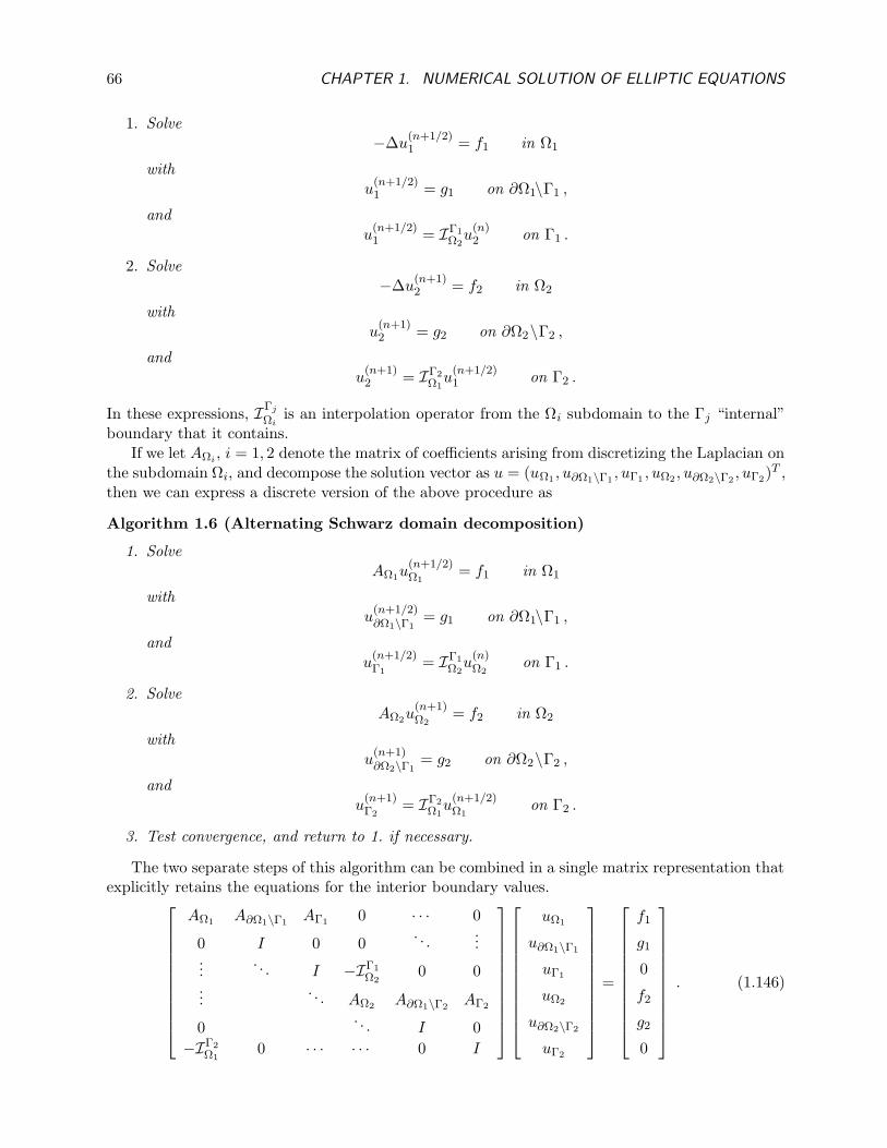
66 CHAPTER 1. NUMERICAL SOLUTION OF ELLIPTIC EQUATIONS
1. Solve−∆u
(n+1/2)1 = f1 in Ω1
withu
(n+1/2)1 = g1 on ∂Ω1\Γ1 ,
andu
(n+1/2)1 = IΓ1
Ω2u
(n)2 on Γ1 .
2. Solve−∆u
(n+1)2 = f2 in Ω2
withu
(n+1)2 = g2 on ∂Ω2\Γ2 ,
andu
(n+1)2 = IΓ2
Ω1u
(n+1/2)1 on Γ2 .
In these expressions, IΓj
Ωiis an interpolation operator from the Ωi subdomain to the Γj “internal”
boundary that it contains.If we let AΩi , i = 1, 2 denote the matrix of coefficients arising from discretizing the Laplacian on
the subdomain Ωi, and decompose the solution vector as u = (uΩ1 , u∂Ω1\Γ1, uΓ1 , uΩ2 , u∂Ω2\Γ2
, uΓ2)T ,
then we can express a discrete version of the above procedure as
Algorithm 1.6 (Alternating Schwarz domain decomposition)
1. SolveAΩ1u
(n+1/2)Ω1
= f1 in Ω1
withu
(n+1/2)∂Ω1\Γ1
= g1 on ∂Ω1\Γ1 ,
andu
(n+1/2)Γ1
= IΓ1Ω2
u(n)Ω2
on Γ1 .
2. SolveAΩ2u
(n+1)Ω2
= f2 in Ω2
withu
(n+1)∂Ω2\Γ1
= g2 on ∂Ω2\Γ2 ,
andu
(n+1)Γ2
= IΓ2Ω1
u(n+1/2)Ω1
on Γ2 .
3. Test convergence, and return to 1. if necessary.
The two separate steps of this algorithm can be combined in a single matrix representation thatexplicitly retains the equations for the interior boundary values.
AΩ1 A∂Ω1\Γ1AΓ1 0 · · · 0
0 I 0 0. . .
......
. . . I −IΓ1Ω2
0 0...
. . . AΩ2 A∂Ω1\Γ2AΓ2
0. . . I 0
−IΓ2Ω1
0 · · · · · · 0 I
uΩ1
u∂Ω1\Γ1
uΓ1
uΩ2
u∂Ω2\Γ2
uΓ2
=
f1
g1
0
f2
g2
0
. (1.146)

1.8. DOMAIN DECOMPOSITION METHODS 67
We have suppressed formal iteration indexing here for brevity, but we now multiply the rows of Eq.(1.146) times the solution vector to obtain the following systems with indexing reinserted.
AΩ1u(n+1/2)Ω1
= f1 − A∂Ω1\Γ1u
(n+1/2)∂Ω1\Γ1
− AΓ1u(n)Γ1
= f1 − A∂Ω1\Γ1g1 − AΓ1IΓ1
Ω2u
(n)Ω2
,
and similarly,
AΩ2u(n+1)Ω2
= f2 − A∂Ω2\Γ1g2 − AΓ2IΓ2
Ω1u
(n+1/2)Ω1
.
We can write these as
u(n+1/2)Ω1
= A−1Ω1
(f1 − A∂Ω1\Γ1
g1 − AΓ1IΓ1Ω2
u(n)Ω2
)
u(n+1)Ω2
= A−1Ω2
(f2 − A∂Ω2\Γ2
g2 − AΓ2IΓ2Ω1
u(n+1/2)Ω1
).
Then addition and subtraction of the appropriate u(n)Ωi
on the right-hand side of each leads to
u(n+1/2)Ω1
= u(n)Ω1
+ A−1Ω1
(f1 − AΩ1u
(n)Ω1
− A∂Ω1\Γ1g1 − AΓ1IΓ1
Ω2u
(n)Ω2
), (1.147a)
u(n+1)Ω2
= u(n)Ω2
+ A−1Ω2
(f2 − AΩ2u
(n)Ω2
− A∂Ω2\Γ2g2 − AΓ2IΓ2
Ω1u
(n+1/2)Ω1
). (1.147b)
We now observe that since the last two terms on the right-hand side of each of these equations areknown, we can define
fi ≡ fi − A∂Ωi\Γjgi − AΓiIΓi
Ωju
(n)Ωj
, i = 1, 2; j = 2, 1 ,
by replacing u(n+1/2)Ω1
with u(n)Ω1
in the second equation. This leads to
u(n+1/2)Ω1
= u(n)Ω1
+ A−1Ω1
(f1 − AΩ1u
(n)Ω1
), (1.148a)
u(n+1)Ω2
= u(n)Ω2
+ A−1Ω2
(f2 − AΩ2u
(n)Ω2
), (1.148b)
which has the formal structure of a preconditioned Richardson iteration; at the same time, it canbe seen that Eq. (1.147) is equivalent to a block Gauss-Seidel procedure. Moreover, it is clear thatresiduals appear in both of these systems, and in this sense they are closely related to the fine-gridupdates by defect equation results in multigrid methods.
An important observation to make at this point is that the grid point values in the overlapregion of Fig. 1.21 must be computed twice for each complete iteration (as was the case with simplerexample provided earlier in connection with ADI implementations) in order to generate all necessaryinternal boundary data. Obviously, this can represent a significant amount of arithmetic in somecases, and beyond this is the fact that unless the simple Richardson formulation of Eq. (1.148)is used, it is not possible to parallelize the algorithm (although the chosen solution procedure(s)within the algorithm might be parallelized)—a situation similar to that of multigrid methods.
This leads us to seek modifications that will make the overall algorithm more efficient. It isclear from Fig. 1.21 that if we did not require overlap between the two subdomains Ω1 and Ω2
beyond the interior boundary Γ1, much less calculation would be required. Moreover, if we could insome manner obtain the solution values on Γ1 independently, then parallelization of the remainingalgorithm would be easy. In the next subsection we treat a method that in principle allows us toaccomplish both of these goals, but which is itself not directly related to Schwarz methods. In alater subsection we will see modifications to Algorithm 1.6 that will achieve similar results.
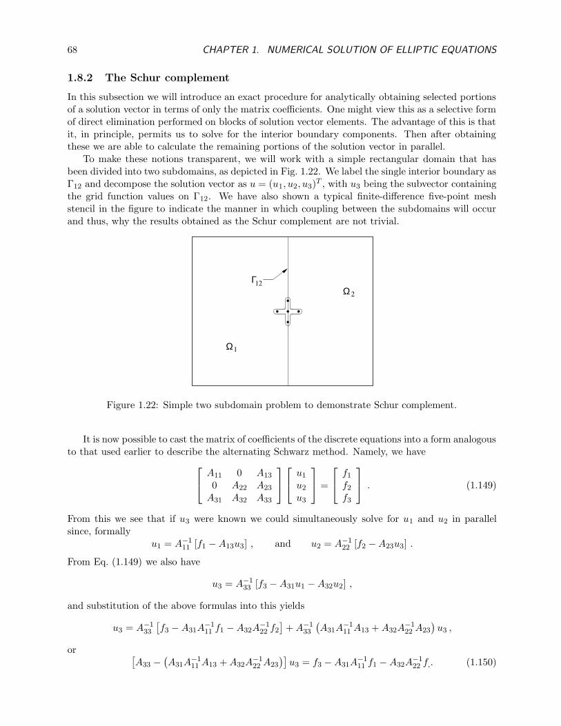
68 CHAPTER 1. NUMERICAL SOLUTION OF ELLIPTIC EQUATIONS
1.8.2 The Schur complement
In this subsection we will introduce an exact procedure for analytically obtaining selected portionsof a solution vector in terms of only the matrix coefficients. One might view this as a selective formof direct elimination performed on blocks of solution vector elements. The advantage of this is thatit, in principle, permits us to solve for the interior boundary components. Then after obtainingthese we are able to calculate the remaining portions of the solution vector in parallel.
To make these notions transparent, we will work with a simple rectangular domain that hasbeen divided into two subdomains, as depicted in Fig. 1.22. We label the single interior boundary asΓ12 and decompose the solution vector as u = (u1, u2, u3)
T , with u3 being the subvector containingthe grid function values on Γ12. We have also shown a typical finite-difference five-point meshstencil in the figure to indicate the manner in which coupling between the subdomains will occurand thus, why the results obtained as the Schur complement are not trivial.
Γ12
Ω1
Ω2
Figure 1.22: Simple two subdomain problem to demonstrate Schur complement.
It is now possible to cast the matrix of coefficients of the discrete equations into a form analogousto that used earlier to describe the alternating Schwarz method. Namely, we have
A11 0 A13
0 A22 A23
A31 A32 A33
u1
u2
u3
=
f1
f2
f3
. (1.149)
From this we see that if u3 were known we could simultaneously solve for u1 and u2 in parallelsince, formally
u1 = A−111 [f1 − A13u3] , and u2 = A−1
22 [f2 − A23u3] .
From Eq. (1.149) we also have
u3 = A−133 [f3 − A31u1 − A32u2] ,
and substitution of the above formulas into this yields
u3 = A−133
[f3 − A31A
−111 f1 − A32A
−122 f2
]+ A−1
33
(A31A
−111 A13 + A32A
−122 A23
)u3 ,
or [A33 −
(A31A
−111 A13 + A32A
−122 A23
)]u3 = f3 − A31A
−111 f1 − A32A
−122 f,. (1.150)
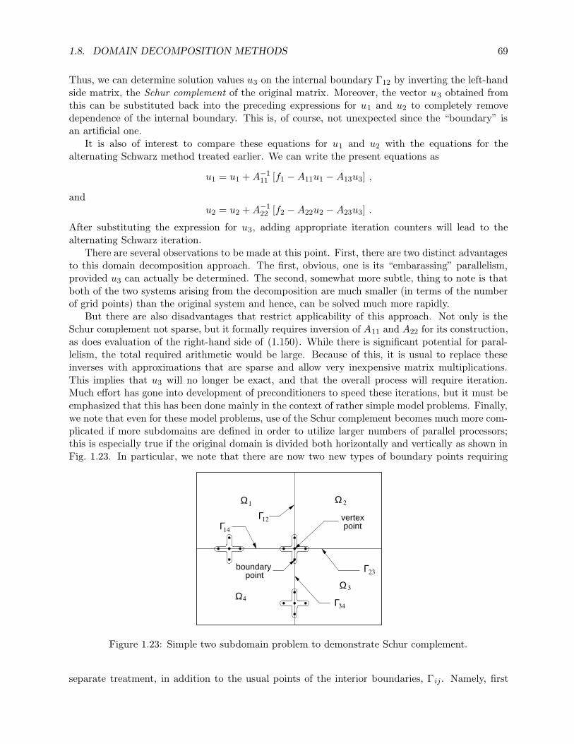
1.8. DOMAIN DECOMPOSITION METHODS 69
Thus, we can determine solution values u3 on the internal boundary Γ12 by inverting the left-handside matrix, the Schur complement of the original matrix. Moreover, the vector u3 obtained fromthis can be substituted back into the preceding expressions for u1 and u2 to completely removedependence of the internal boundary. This is, of course, not unexpected since the “boundary” isan artificial one.
It is also of interest to compare these equations for u1 and u2 with the equations for thealternating Schwarz method treated earlier. We can write the present equations as
u1 = u1 + A−111 [f1 − A11u1 − A13u3] ,
andu2 = u2 + A−1
22 [f2 − A22u2 − A23u3] .
After substituting the expression for u3, adding appropriate iteration counters will lead to thealternating Schwarz iteration.
There are several observations to be made at this point. First, there are two distinct advantagesto this domain decomposition approach. The first, obvious, one is its “embarassing” parallelism,provided u3 can actually be determined. The second, somewhat more subtle, thing to note is thatboth of the two systems arising from the decomposition are much smaller (in terms of the numberof grid points) than the original system and hence, can be solved much more rapidly.
But there are also disadvantages that restrict applicability of this approach. Not only is theSchur complement not sparse, but it formally requires inversion of A11 and A22 for its construction,as does evaluation of the right-hand side of (1.150). While there is significant potential for paral-lelism, the total required arithmetic would be large. Because of this, it is usual to replace theseinverses with approximations that are sparse and allow very inexpensive matrix multiplications.This implies that u3 will no longer be exact, and that the overall process will require iteration.Much effort has gone into development of preconditioners to speed these iterations, but it must beemphasized that this has been done mainly in the context of rather simple model problems. Finally,we note that even for these model problems, use of the Schur complement becomes much more com-plicated if more subdomains are defined in order to utilize larger numbers of parallel processors;this is especially true if the original domain is divided both horizontally and vertically as shown inFig. 1.23. In particular, we note that there are now two new types of boundary points requiring
vertex point
boundary point
Ω1 Ω 2
Ω3Ω4
Γ12Γ14
Γ23
Γ34
Figure 1.23: Simple two subdomain problem to demonstrate Schur complement.
separate treatment, in addition to the usual points of the interior boundaries, Γij. Namely, first

70 CHAPTER 1. NUMERICAL SOLUTION OF ELLIPTIC EQUATIONS
are points having the property that each occurs in the calculations of two distinct boundaries; wehave termed these simply “boundary points.” Second, in the case displayed in Fig. 1.23 there is asingle point associated with all four interior boundaries; these are called “vertex points.” Each ofthese types requires special treatment.
1.8.3 Multiplicative and additive Schwarz methods
Now that we have seen a formal procedure for expressing internal boundary values directly via theSchur complement, we will now return to the Schwarz-like methods to find what are essentiallyapproximations to the Schur complement. It is clear from the preceding that this will be necessaryfor computational efficiency. What is at question is whether good approximations can be foundthat do not destroy parallelism. As we have noted earlier, there are two main classes of Schwarz-likeprocedures by means of which the prominent overlap of the alternating Schwarz method can bereduced. These are multiplicative and additive Schwarz techniques; we will describe each of thesein what follows.
Multiplicative Schwarz method
Consider a domain such as the one depicted in Fig. 1.22 used to study the Schur complement, butnow permit some overlap, as shown in Fig. 1.24, part (a). We will assume that discretization hasresulted in matched grids so that no interpolation operators will be needed to transfer information
Ω1
Γ12Γ
2Ω
∪2ΩΩ1
Ω1A
Ω 2A
Ω1u
Ω2u
∪2ΩΩ1u
(a) (b)
Figure 1.24: Domain decomposition with two overlapping subdomains; (a) domain geometry, (b)matrix structure.
between domains.If we absorb boundary data into the fis as done previously, but now suppress the tilde notation,
we can obtain equations similar in form to those given earlier in the context of alternating Schwarz

1.8. DOMAIN DECOMPOSITION METHODS 71
methods:
u(n+1/2)Ω1
= u(n)Ω1
+ A−1Ω1
(f1 − AΩ1u
(n)Ω1
− AΓ1u(n)Γ1
),
u(n+1)Ω2
= u(n)Ω2
+ A−1Ω2
(f2 − AΩ2u
(n)Ω2
− AΓ2u(n+1/2)Γ2
).
It is clear that the overlap region is again being computed twice with each complete iteration,and that this formulation is equivalent to the block Gauss-Seidel methods. We also observe thatdependence on the interior boundaries can be formally removed by expressing these equations as
u(n+1/2)Ω1
= u(n)Ω1
+ A−1Ω1
(f1 − AΩ1u
(n)Ω1
− AΩ\Ω1u
(n)Ω\Ω1
), (1.151a)
u(n+1)Ω2
= u(n)Ω2
+ A−1Ω2
(f2 − AΩ2u
(n)Ω2
− AΩ\Ω2u
(n+1/2)Ω\Ω2
). (1.151b)
It should be emphasized, however, that interior boundary dependence is not truly removed, but
rather buried in the notation; viz., the solution on these boundaries is contained in u(n)Ω\Ω1
and
u(n)Ω\Ω2
.
To gain further insight into the workings of the multiplicative Schwarz methods (and amongother things, see whence the terminology arose) it is useful to construct the fixed-point form of thistechnique. We begin by introducing the formal representation
u(n+1/2) = u(n) +
(A−1
Ω10
0 0
)(f − Au(n)
), (1.152a)
u(n+1) = u(n+1/2) +
(0 0
0 A−1Ω2
)(f − Au(n+1/2)
). (1.152b)
It is important to recognize that, despite the notation, during each half step only that portion ofthe solution vector is updated as is indicated by the portion of the original matrix used in that step.It should also be noted that the form, while still basically a Gauss-Seidel iteration, is somewhatdifferent than that used previously; in particular, the current form is, in some sense, closer to whatwe usually call Gauss-Seidel iteration than was the previous block form.
We will now introduce some definitions and notation to aid in constructing the fixed-point formof the overall domain decomposition procedure. We first define restrictions (similar to injections inthe multigrid sense) via
uΩ1 ≡ R1u = (I, 0)
(uΩ1
uΩ\Ω1
),
and
uΩ2 ≡ R2u = (0, I)
(uΩ\Ω2
uΩ2
).
From this it is easily seen that
AΩi = RiARTi , i = 1, 2 , (1.153)
since the identity matrix appearing in each Ri is just the right size to pick out the correspondinguΩi . It is also important to note that the Ris can be defined simply in terms of an index set—nomatrix Ri is stored, and certainly we would not actually perform a multiplication to constract uΩi .
Now defineBi = RT
i
(RiART
i
)−1 Ri , i = 1, 2 . (1.154)
72 CHAPTER 1. NUMERICAL SOLUTION OF ELLIPTIC EQUATIONS
These matrices correspond to the following sequence of steps: i) restrict the residual to one subdo-main; ii) solve the problem on that subdomain to generate a correction, and then iii) prolongatethe correction back to the whole domain. (The similarities to multigrid are quite pronounced.)Again, we note that in practical calculations these matrices are never actually formed; they merelyprovide a conceptual representation for analysis of the method.
We can now use these definitions in the earlier formulas for the multiplicative Schwarz methodto obtain
u(n+1/2) = u(n) + RT1
(R1ART
1
)−1R1
(f − Au(n)
),
u(n+1) = u(n+1/2) + RT2
(R2ART
2
)−1R2
(f − Au(n+1/2)
),
or
u(n+1/2) = u(n) + B1
(f − Au(n)
), (1.155a)
u(n+1) = u(n+1/2) + B2
(f − Au(n+1/2)
). (1.155b)
Combining these two steps in the usual way yields
u(n+1) = u(n) + B1
(f − Au(n)
)+ B2
[f − A
(u(n) + B1
(f − Au(n)
))]
= u(n) + [B1 + B2 − B2AB1](f − Au(n)
).
This can be easily rearranged to obtain the usual form of a linear fixed-point iteration,
u(n+1) = Gu(n) + k ,
where now
G ≡ I − (B1 + B2 − B2AB1)A , (1.156)
k ≡ (B1 + B2 − B2AB1) f . (1.157)
It is of interest to observe that this formula for the iteration matrix G can be factored to obtain
G = (I − B1A) (I − B2A) ,
and it is from this product form that the terminology multiplicative Schwarz iteration arises.
Additive Schwarz method
As we have emphasized from the start of our discussion of multiplicative Schwarz methods, theyare basically block Gauss-Seidel iterations; as such they are not as easily parallelized as would beblock Jacobi iterations. Despite the fact that Gauss-Seidel can be expected to be more rapidlyconvergent, it is possible that improved parallelization would more than make up for this, and thishas motivated study of the so-called additive Schwarz procedures. The fixed-point form of thesemethods can be obtained as follows.
First recall Eq. (1.152) and replace all entries of u(n+1/2) on the right-hand side with u(n).Clearly, this is then a block Jacobi iteration in the same sense that (1.152) is Gauss-Seidel iteration.We can now simply write these two steps as a single equation to obtain
u(n+1) = u(n) +
[(A−1
Ω10
0 0
)+
(0 0
0 A−1Ω2
)](f − Au(n)
),
1.8. DOMAIN DECOMPOSITION METHODS 73
or upon using Eqs. (1.153) and (1.154),
u(n+1) = u(n) + (B1 + B2)(f − Au(n)
). (1.158)
This is easily rearranged to obtain the usual fixed-point form from which the definitions
G ≡ I − (B1 + B2)A , (1.159)
andk = (B1 + B2) f (1.160)
follow. It is clear that the formula for G cannot be factored as it could in the multiplicative Schwarzcase, so the present form is termed the additive Schwarz procedure.
Comparison of Schwarz methods
From the standpoint of parallelization the advantage of additive Schwarz over all of the othertechniques we have considered is quite clear. Application of the two matrices B1 and B2 (note thatthis is simply yet another case of preconditioning) can easily be performed in parallel. On the otherhand, the analogy between Gauss-Seidel (multiplicative Schwarz) and Jacobi (additive Schwarz)iterations suggests that the former should converge twice as fast as the latter. Indeed, this is borneout in the numerical experiments presented in Smith et al. [37]. These were performed with thefollowing model problem solved with two subdomains similar to what is shown in Fig. 1.22.
−∆u = xey in Ω ≡ (0, 2) × (0, 1) ,
with Dirichlet conditionsu = −xey on ∂Ω .
The results reported in [37] are repeated here in the following table.
Table 1. Comparison of alternating, multiplicative and additive Schwarz methods.
# of grid points
overlap alternating multiplicative additive
123123123
11×6
21×11
31×16
7 5 413 7 51910 7
222322332
433544554
It is easily seen from the table that the expected relationship between multiplicative and additiveSchwarz convergence rates is observed; moreover neither is very sensitive to either the amount ofoverlap or the number of points in the grid. On the other hand, it is clear that the alternatingSchwarz method is fairly sensitve to both of these—especially, the former. But it is importantto be aware of the context of these results. The computations were performed with an error
74 CHAPTER 1. NUMERICAL SOLUTION OF ELLIPTIC EQUATIONS
tolerance of only 10−2, which not only is quite large, but it was applied only to the error-reductionfactor; i.e., when the initial error had been reduced to 1% of its original amount, the iterationswere declared converged. In fact, almost any method will perform fairly well with such a coarsetolerance because the number of iterations required to achieve this is often sufficiently small thatonly high-wavenumber errors have been removed, and the method has not yet reached its asymptoticbehavior. Moreover, the grids in these cases contain so few points that the results can in no waybe considered asymptotic. Thus, the contents of Table 1. must be viewed with caution. Indeed, itis by now widely accepted that the basic domain decomposition methods discussed to this pointare not extremely effective for finely-gridded problems.
Schwarz methods in the context of many subdomains
We will now briefly describe how the preceding results can be extended to the case of p sub-domains. We will demonstrate this specifically for the case of multiplicative Schwarz methods; theadditive case is actually easier, as the reader should by now recognize.
We suppose the solution domain has been subdivided into p subdomains and write the equationsconstituting the multiplicative Schwarz procedure as
u(n+1/p) = u(n) + B1
(f − Au(n)
)
u(n+2/p) = u(n+1/p) + B2
(f − Au(n+1/p)
)
...
u(n+1) = u(n+ p−1p
) + Bp
(f − Au(n+ p−1
p))
,
where, as in Eq. (1.154), Bi = RTi
(RiART
i
)Ri.
It is worth noting here that details of the subdomain geometric structures are not important inthis representation because the Ris are constructed to account for these. It is also useful to considerthe effects of such a decomposition on the performance of any typical iterative solver employed oneach of the p subdomains. Suppose Ω =
⋃pi=1 Ωi has been discretized with uniform grid spacing h
and that each of the p subdomains is of size H with h < H < min(a, b), where Ω is the rectangle(0, a) × (0, b). Now recall the form of the spectral radius for Jacobi iterations given earlier in thissection, and also as Eq. (1.39); namely,
ρ(B) = 1 − 1
4
[(π
a
)2+(π
b
)2]
h2 .
We note that ρ(L) for Gauss-Seidel iterations is simply the square of this quantity, and thatρ(Lωb
) for optimal SOR is also closely related. We see that replacing a and b with H in thisexpression results in a significant decrease in the size of ρ(B) if H is sufficiently small, and thusin the performance of the iteration scheme. On the other hand, solutions from these individualsubdomains must be iteratively combined to construct the complete solution.
We can qualitatively characterize convergence of this iterative process, and hence that of theSchwarz procedures, as follows (see [37] and references therein for more details): let h and H be asabove, and let δ denote the width of overlap between subdomains. Then
i) the number of required iterations grows as 1/H;
ii) if δ is kept proportional to H, the number of iterations is bounded independently of h andH/h;
1.8. DOMAIN DECOMPOSITION METHODS 75
iii) the number of iterations needed for multiplicative Schwarz is approximately one half of thatrequired by additive Schwarz;
iv) convergence is poor if δ = 0 (no overlap) but improves rapidly with increasing δ.
We should note that point i) above might seem to contradict the conclusions reached in ourpreceding discussion of effects of spectral radius for solvers on the subdomains. But, in fact, it arisesdue to a different effect, alluded to above. Namely, as H decreases the number of subdomains, andhence the number of subdomain boundaries, must increase; this makes the problem of piecingtogether the subdomain solutions more difficult. We will consider this from a somewhat differentviewpoint below.
Point ii) provides a means by which domain decomposition converges at a rate independentof grid spacing, and it works in a manner rather analogous to adding levels in a FMG method asgrid spacing is refined. Point iii) is especially important, for it implies that on multiprocessors thesimpler additive Schwarz methods will generally be at least as effective as are the multiplicativeSchwarz procedures. Indeed, the latter cannot be parallelized without “coloring” the subdomains.In the absence of coloring, a two-subdomain decomposition can be calculated in roughly equaltimes by the two approaches; moreover, if p>2 the additive Schwarz methods will be more efficientprovided there are more than two processors available. Finally, point iv) should also be noted.Clearly, some overlap is extremely important, but it has been found that generally no more thantwo or three grid lines are needed for significant improvements in convergence rates, and beyondthis further increases in overlap are generally not useful.
1.8.4 Multilevel domain decomposition methods
We conclude this introduction to domain decomposition methods with a brief discussion of so-called multilevel domain decomposition which actually corresponds to a combination of multigridand domain decomposition methods, as will be evident from what follows. The motivation for thisapproach is the need to remove low-wavenumber errors, as is done in multigrid methods. But theinterpretation of this problem is now somewhat different. In particular, we have already seen thatdomain decompositions reduce the spectral radius of the iteration matrices used in each subdomainin a way that is complementary to what multigrid methods accomplish. On the other hand, becausecomputations are never done on a coarse grid in the usual single-level domain decompositions,boundary information from the actual problem geometry propagates to the interior of the domainsomewhat slowly. This can be improved with the use of a coarse grid in conjunction with the finegrid on which the accurate calculations are performed.
We begin by noting that the preconditioning matrices Bi introduced earlier have analogues inmultigrid procedures. To see this, recall that the multigrid coarse-grid correction is carried outvia the following steps: i) restriction of the fine-grid residual, ii) coarse-grid solution of the defectequation, and iii) prolongation of the coarse-grid error back to the fine grid. We also noted thattypical restriction operators are transposes of a corresponding prolongation. Thus,
BC = RT A−1C R
(where AC = RART ) provides a preconditioner embodying all the components of a coarse-gridcorrection. Clearly, this is of the same general form as the domain decomposition preconditionerdiscussed in the previous section if we appropriately interpret A−1
C and at the same time recognizethat the details of restriction (and prolongation) are rather different in the multigrid case.
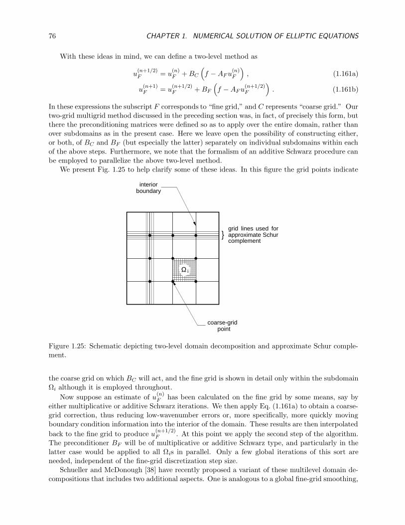
76 CHAPTER 1. NUMERICAL SOLUTION OF ELLIPTIC EQUATIONS
With these ideas in mind, we can define a two-level method as
u(n+1/2)F = u
(n)F + BC
(f − AF u
(n)F
), (1.161a)
u(n+1)F = u
(n+1/2)F + BF
(f − AF u
(n+1/2)F
). (1.161b)
In these expressions the subscript F corresponds to “fine grid,” and C represents “coarse grid.” Ourtwo-grid multigrid method discussed in the preceding section was, in fact, of precisely this form, butthere the preconditioning matrices were defined so as to apply over the entire domain, rather thanover subdomains as in the present case. Here we leave open the possibility of constructing either,or both, of BC and BF (but especially the latter) separately on individual subdomains within eachof the above steps. Furthermore, we note that the formalism of an additive Schwarz procedure canbe employed to parallelize the above two-level method.
We present Fig. 1.25 to help clarify some of these ideas. In this figure the grid points indicate
interiorboundary
coarse-grid point
grid lines used for approximate Schur complement
Ω i
Figure 1.25: Schematic depicting two-level domain decomposition and approximate Schur comple-ment.
the coarse grid on which BC will act, and the fine grid is shown in detail only within the subdomainΩi although it is employed throughout.
Now suppose an estimate of u(n)F has been calculated on the fine grid by some means, say by
either multiplicative or additive Schwarz iterations. We then apply Eq. (1.161a) to obtain a coarse-grid correction, thus reducing low-wavenumber errors or, more specifically, more quickly movingboundary condition information into the interior of the domain. These results are then interpolated
back to the fine grid to produce u(n+1/2)F . At this point we apply the second step of the algorithm.
The preconditioner BF will be of multiplicative or additive Schwarz type, and particularly in thelatter case would be applied to all Ωis in parallel. Only a few global iterations of this sort areneeded, independent of the fine-grid discretization step size.
Schueller and McDonough [38] have recently proposed a variant of these multilevel domain de-compositions that includes two additional aspects. One is analogous to a global fine-grid smoothing,
1.8. DOMAIN DECOMPOSITION METHODS 77
but is intended mainly to aid in globally coupling the subdomain solutions, and the second is anapproximate Schur complement calculation that provides much more accurate boundary data forthe interior boundaries. Otherwise, the structure of the algorithm is quite similar to what we havealready discussed.
Just as in a typical multigrid method, the fine-grid smoothing is performed as the first step ofthe current iteration. Following this, the approximate Schur complements are constructed for allinterior boundaries by applying SLOR on each such boundary and a few of the nearest-neighborgrid lines, as indicated in Fig. 1.25. Clearly, all such solves can be performed in parallel in eachseparate direction (there is a parallelization issue with vertex points if all lines in both directionsare done simultaneously). Once these boundary values have been computed, all subdomains canbe computed in parallel if the additive Schwarz procedure is employed.
These two added steps require minimal arithmetic per pass through the complete algorithm.The fine-grid smoothing is done for only a few iterations, and calculation of the approximate Shurcomplements requires less than one fine-grid smoothing operation for all boundaries combined.Moreover, the latter provides additional overlap even though the domain decomposition, per se,has only one common line of data for every pair of adjacent subdomains.
Preliminary results [38] for a model Poisson-Dirichlet problem have been very encouraging,indicating that total arithmetic scales as O(N) even for extremely large problems (up to > 2.5×10⁶
grid points). But in addition, the overall parallelizability of the method is such as to yield run timesthat are independent of problem size provided there are sufficient processors available to permitlinear increase in number of processors with the number of subdomains.

78 CHAPTER 1. NUMERICAL SOLUTION OF ELLIPTIC EQUATIONS
Chapter 2
Time-Splitting Methods for Evolution
Equations
In this chapter we will treat the numerical solution of time-dependent partial differential equations,mainly of parabolic type (but often employing techniques that apply equally well to hyperbolicequations). As was the case in Chap. 1, we will consider problems consisting of only a single, linearequation, and posed on rectangular domains of two and three spatial dimensions.
We will concentrate our efforts on so-called time-splitting methods for solving such problems,in the context of finite-difference (or finite-volume) discretizations. This is by far the most effi-cient combination for general (having not necessarily smooth solutions) problems. Time-splittingprocedures are often termed “method of fractional steps,” especially in the Russian literature, andthey are frequently referred to simply as “ADI methods.” In the present lectures we will identifythree distinct classes of time-splitting techniques based, not necessarily on their final form (whichtends to almost always be nearly the same), but rather on the manner in which they will have beenconstructed. These are: i) alternating direction implicit (ADI), ii) locally one-dimensional (LOD)and iii) general Douglas-Gunn (D-G). A section of this chapter will be devoted to treatment ofeach of these.
We will consider as a basic model for all methods, the 2-D transient heat equation on a rectangle:
ut = ∆u + f(x, y, t) (x, y) ∈ Ω ≡ (0, a) × (0, b) , t ∈ (0, tf ] , (2.1a)
with initial data
u(x, y, 0) = u0(x, y) , (2.1b)
and boundary conditions
u(x, y, t) = g(x, y, t), (x, y) ∈ ∂Ω . (2.1c)
This problem is particularly simple, and exact solutions are readily constructed. It thus providesa good reference point by means of which performance of the various classes of methods can becompared.
We emphasize at the outset that the reason for the efficiency of time-splitting is that multi-dimensional problems are decomposed into sequences of 1-D problems via this approach. These are,of course, easily solved (and easily parallelized, at least in principle). But the requirement for accom-plishing time splitting is that the system matrix corresponding to the complete multi-dimensionalsystem be sparse and banded, and with very regular band structure. It is this requirement thatleads to difficulty for finite-element methods, and even for finite-difference methods constructed onunstructured grids.
79
80 CHAPTER 2. TIME-SPLITTING METHODS FOR EVOLUTION EQUATIONS
2.1 Alternating Direction Implicit Methods
We have already discussed ADI methods for solving elliptic problems in Chap. 1 of these lectures,but the treatment there (as we had noted at that time) was rather different from the time-dependentanalysis we will now study. We note that there are three main steps in constructing an ADI methodin this context: i) discretization of the partial differential equation, ii) factorization of the discreteequation and iii) splitting of the factored equations. It is important to recognize that error will beintroduced with each one of these steps, and in order to assess the overall accuracy of any givenADI scheme it will be necessary to analyze each such error contribution. We will carry this outfor the model problem in the context of the Peaceman-Rachford method [16], and then provide asimple analysis of stability for this approach. We will then briefly consider a second widely-usedADI scheme, and then conclude the section with some implementation details.
2.1.1 Peaceman-Rachford ADI
In this section we will derive the Peaceman-Rachford alternating direction implicit scheme for 2-D parabolic equations, and in the course of doing this analyze error contributions from each ofthe individual steps. We emphasize that this method can be applied only to 2-D problems, butwe present it here because it provides a good tool for studying the ADI construction process ingeneral.
Accuracy
The discretization we employ here is the well-known Crank-Nicolson method (see, e.g., Mitchelland Griffiths [9]) which in 2D takes the form
[I − k
2
(D2
0,x + D20,y
)]un+1
`,m =
[I +
k
2
(D2
0,x + D20,y
)]un
`,m +k
2
(fn+1
`,m + fn`,m
). (2.2)
This difference equation holds for all ` = 2, 3, . . . , Nx − 1 and m = 2, 3, . . . , Ny − 1; the boundarypoint values corresponding to the indices ` = 1, Nx and m = 1, Ny are prescribed as indicated inEq. (2.1c). Also note that in these lectures the notation D0,· will be used to indicate a second-orderaccurate centered-difference approximation, and k denotes the time step value, i.e., ∆t (≡ tn+1−tn).This approximation is well-known to be second-order in both space and time, as may be easilychecked via a formal truncation error analysis, which we leave to the reader.
To simplify notation, we set A ≡ D20,x and B ≡ D2
0,y and write
[I − k
2(A + B)
]un+1 =
[I +
k
2(A + B)
]un +
k
2(fn+1 + fn) , (2.3)
where we have now suppressed spatial grid-point indices in favor of the more compact matrix-vectorrepresentations. We remark that structure of the matrix on the left-hand side of the above equationis that of a discrete Laplacian. Hence, solution of the system is expensive—and it must be donemany times in the case of time-dependent problems. We have seen in the preceding chapter thatrather complicated algorithms are needed to obtain solutions in only O(N) arithmetic; moreover,the actual total amount of arithmetic still is fairly large. This provides the motivation for techniqueswe consider in this chapter.
Our task now is to factor the matrices on both sides of Eq. (2.3). This can be done by observingthat (
I − k
2A
)(I − k
2B
)= I − k
2(A + B) +
k2
4AB .

2.1. ALTERNATING DIRECTION IMPLICIT METHODS 81
Thus, the factorization on the left-hand side agrees with the matrix on the left-hand side of (2.3) upto terms of O(k2). A similar result holds for the right-hand-side matrix of (2.3), and substitutionof these back into Eq. (2.3) yields[(
I − k
2A
)(I − k
2B
)− k2
4AB
]un+1 =
[(I +
k
2A
)(I +
k
2B
)− k2
4AB
]un +
k
2
(fn+1 + fn
),
or(
I − k
2A
)(I − k
2B
)un+1 =
(I +
k
2A
)(I +
k
2B
)un +
k
2
(fn+1 + fn
)+
k2
4AB
(un+1 − un
).
(2.4)Now recall that the original unsplit Crank-Nicolson scheme has O(k3) local temporal error, so
at first it appears that the factorization has resulted in a reduction of order of accuracy. But ifu ∈ C1, the mean value theorem implies that
un+1 − un = ut(ξ)(tn+1 − tn
)for some ξ ∈
(tn, tn+1
),
from which it follows that un+1 − un ∼ O(k). Hence, no formal accuracy has been lost in thefactorization given by (2.4). But we must also note that we have not yet gained any simplificationof the solution procedure.
To accomplish this simplification we must now carry out the splitting step. There are numerousways by which this can be done; here we will employ the Peaceman-Rachford (P-R) method [16],and write (2.4) as the system of equations
(I − k
2A
)un+1∗ =
(I +
k
2B
)un +
k
2fn , (2.5a)
(I − k
2B
)un+1 =
(I +
k
2A
)un+1∗ +
k
2fn+1 , (2.5b)
where un+1∗ corresponds to an intermediate time t∗, tn ≤ t∗ ≤ tn+1. In many presentations of theP-R method it is assumed that t∗ = tn+1/2; this is not always correct in general, despite the factthat it is necessary for maintaining consistency of the individual split equations. It is importantto note at this time that both Eqs. (2.5a) and (2.5b) correspond to tridiagonal systems, and thuscan be solved very efficiently. Hence, we have produced the desired simplification. But we mustyet determine the error caused by splitting.
To analyze the formal accuracy of P-R ADI we will attempt to recover the factored form of theCrank-Nicolson scheme (because we already know the accuracy of this method) using Eq. (2.5),and note the difference between these two results. We begin by solving Eq. (2.5a) for un+1∗ andsubstituting the result into Eq. (2.5b) to obtain(
I − k
2B
)un+1 =
(I +
k
2A
)[(I − k
2A
)−1(I +
k
2B
)un +
k
2
(I − k
2A
)−1
fn
]+
k
2fn+1
=
(I +
k
2A
)(I − k
2A
)−1[(I +
k
2B
)un +
k
2fn
]+
k
2fn+1 . (2.6)
At this point we should recognize that if we are to recover anything that resembles (2.4) we needto multiply by
(I − k
2A); this leads to
(I − k
2A
)(I − k
2B
)un+1 =
(I − k
2A
)(I +
k
2A
)(I − k
2A
)−1[(I +
k
2B
)un +
k
2fn
]
+k
2
(I − k
2A
)fn+1 .
(2.7)
82 CHAPTER 2. TIME-SPLITTING METHODS FOR EVOLUTION EQUATIONS
We now observe that I − k2A and I + k
2A commute (provided A is independent of time), so (2.7)becomes(
I − k
2A
)(I − k
2B
)un+1 =
(I +
k
2A
)(I +
k
2B
)un +
k
2
(I +
k
2A
)fn +
k
2
(I − k
2A
)fn+1
=
(I +
k
2A
)(I +
k
2B
)un +
k
2
(fn+1 + fn
)− k2
4A(fn+1 − fn
). (2.8)
From this we see that if A is independent of time, and f ∈ C 1(t0, tf ), so that
fn+1 − fn = ft(ξ)(tn+1 − tn
)∼ O(k) ,
then (2.8) is equivalent to (2.4) up to terms of O(k3).Since this is the order of the local truncation error of the unsplit Crank-Nicolson scheme, we
have shown that the formal accuracy of P-R ADI is equivalent to that of Crank-Nicolson for the2-D heat equation with C1 source term, despite the much higher solution efficiency gained fromthe time splitting.
Stability
At this time we briefly analyze stability of time-split schemes, but mainly in the context of theP-R method just presented. It is useful to note that all of the time-split methods we will considerherein are implicit (although explicit time-splitting is also widely applied), so stability (at least forlinear problems) is typically not a problem. An important property of any time-split method isthat individual steps need be neither consistent nor stable in order for the overall scheme to exhibitthese properties. In some situations this can be a significant advantage.
For the P-R method being considered here, each of the steps is basically a 1-D Crank-Nicolsonscheme, which for linear heat equations is well known to be unconditionally stable with respect toa von Neumann stability analysis (see, e.g., [9]). This implies that the amplification factor for eachindividual step is less than unity, and we then simply need to show that the amplification factorfor the complete method is the product of the amplification factors of the individual steps.
Consider Eq. (2.5) with A = B. We note that this occurs for the heat equation if the samespatial step size is used in both directions. In terms of a matrix stability analysis it is required thatthe spectral radius of
C ≡(
I − k
2A
)−1(I +
k
2B
)
be less than or equal to unity; i.e., ρ(C) ≤ 1, for the first split step to be stable. Similarly, werequire ρ(D) ≤ 1, with
D ≡(
I − k
2B
)−1(I +
k
2A
),
for the second step. Now recall that for any matrix M , ρ(M) ≤ ‖M‖ for all matrix norms ‖ · ‖.Also recall that if we define
zn ≡ vn − un ,
where vn is the exact solution to the difference equations, and un is the computed one, we havethat
zn+1 =
(I − k
2B
)−1(I +
k
2A
)(I − k
2A
)−1(I +
k
2B
)zn . (2.9)
Thus,‖zn+1‖ = ‖DCzn‖ ≤ ‖D‖‖C‖‖zn‖ .
2.1. ALTERNATING DIRECTION IMPLICIT METHODS 83
If we now take ‖ · ‖ = ρ(·), which is valid provided that C and D are diagonalizable with realeigenvalues, we have
‖zn+1‖ ≤ ρ(C) · ρ(D)‖zn‖ .
But since C and D are equivalent to matrices arising in the 1-D Crank-Nicolson method, we haveρ(C) ≤ 1 and ρ(D) ≤ 1 for all values of k and h. Hence,
‖zn+1‖ ≤ ‖zn‖ ,
and we have demonstrated (unconditional) stability for the P-R method.
It should be clear from this development that since all that really is needed is ρ(C) · ρ(D) ≤ 1,it is possible for one or the other (but not both) individual split steps to be unstable while stillmaintaining overall stability of the complete method.
2.1.2 Douglas-Rachford ADI
In this section we will briefly treat the Douglas-Rachford [39] ADI scheme. This method is basedon a backward Euler time integration, and so is only first-order accurate in time. But it is uncondi-tionally stable just as was the P-R method, and unlike that method, the Douglas-Rachford (D-R)scheme is easily generalized to three space dimensions. Furthermore, it is worth noting that in somesituations, maintaining high-order accuracy is difficult for boundary condition implementations, souse of a first-order method may be appropriate in any case.
The discretization of the heat equation using backward Euler integration in time and centereddifferencing in space results in
[I − k
(D2
0,x + D20,y
)]un+1 = un + kfn+1 , (2.10)
or in our abbreviated notation,
[I − k (A + B)]un+1 = un + kfn+1 .
The factored form of this is
(I − kA)(I − kB)un+1 = un + fn+1 , (2.11)
and the Douglas-Rachford splitting results in
(I − kA)un+1∗ = (I + kB)un + kfn+1 (2.12a)
(I − kB)un+1 = un+1∗ − kBun . (2.12b)
We leave derivation of the factorization and splitting errors for this method as an exercise for theinterested reader.
As we noted above with regard to the Peaceman-Rachford splitting, there are many possibleways in which this might be carried out once the equation has been factored. But clearly, oneshould always try to produce a splitting which when re-composed will be as close as possible tothe factored but unsplit formulation—or, better yet, as close as possible to the original unfactoreddiscrete form. It is readily seen by formally solving (2.12a) for un+1∗ and substituting this into(2.12b), followed by multiplication by (I − kA) that this has been accomplished by the Douglas-Rachford splitting. It will be seen in a later section that this splitting is the same as that employedin the Douglas-Gunn procedures.
84 CHAPTER 2. TIME-SPLITTING METHODS FOR EVOLUTION EQUATIONS
We will not present details of a stability analysis for this method. Since it is based on backwardEuler integration in time, it is expected to be unconditionally stable for linear problems; and ananalysis similar to that used above for the P-R method will confirm this for the split scheme.Moreover, we note that based on the preceding analysis, we can conclude that stability of the splitscheme is usually at least as good as for the unsplit one. In fact, explicit schemes are sometimessplit specifically to exploit this property of time splitting.
We will close this section by presenting the equations for the D-R procedure applied to a 3-Dheat equation in the homogeneous case:
(I − kD2
0,x
)un+1∗ =
[I + k
(D2
0,y + D20,z
)]un , (2.13a)
(I − kD2
0,y
)un+1∗∗ = un+1∗ − kD2
0,yun , (2.13b)
(I − kD2
0,z
)un+1 = un+1∗∗ − kD2
0,zun . (2.13c)
We leave as an exercise for the interested reader derivation of corresponding formulas in the non-homogeneous case, as well as analysis of the splitting error for this scheme.
2.1.3 Implementation of ADI schemes
In this section we will discuss some of the details that must be understood to successfully implementADI methods. In fact, most of what we will present here carries over to all time-splitting techniques.There are two main items that are of particular importance; these are: i) specific details of carryingout the line-by-line solves and ii) treatment of boundary conditions.
ADI line-by-line solves
One of the advantages of ADI methods from their earliest use was the ability to decompose theglobal solution domain into a sequence of lines, thus permitting solution of the complete PDEproblem as a collection of solutions to problems that were each no larger than ODE two-pointboundary value problems on the same line of grid points. In the modern era of extremely largeCPUs and memories, this is much less an important factor. On the other hand, in instances of smallcache sizes, and/or in the context of parallelization, this feature can still present an advantage overother approaches. In this subsection we will describe the details of implementing these line-by-linesolves, and also briefly describe an alternative.
It is of interest to consider the form of the discrete equation on any arbitrary line of the gridto gain an understanding of some subtle aspects of correct implementation. We will consider theP-R scheme here, although similar requirements arise for most other methods. We will choose anarbitrary line from the first split step, corresponding to Eq. (2.5a), and express this as
−run+1∗
`−1,m + (1 + 2r)un+1∗
`,m − run+1∗
`+1,m = run`,m−1 + (1 − 2r)un
`,m + run`,m+1 +
k
2fn
`,m , (2.14)
where r = k/2h2. An equation of this form holds for each m = 2, 3, . . . , Ny−1 and, with somemodification for boundary conditions, also for m = 1 and m = Ny.
Since the right-hand side is known, the problem is completely analogous to that of solving anODE boundary-value problem along the mth grid line. But the fact that everything on the right-hand side is to be evaluated with time-level n information presents a slight difficulty in terms ofstoring newly-computed results. The problem is indicated graphically in Fig. 2.1, and we describeit here. The important thing to observe is that the results on grid line m−1 at time level n arestill needed for the n+1 time-level calculation at grid line m. But these would typically have been
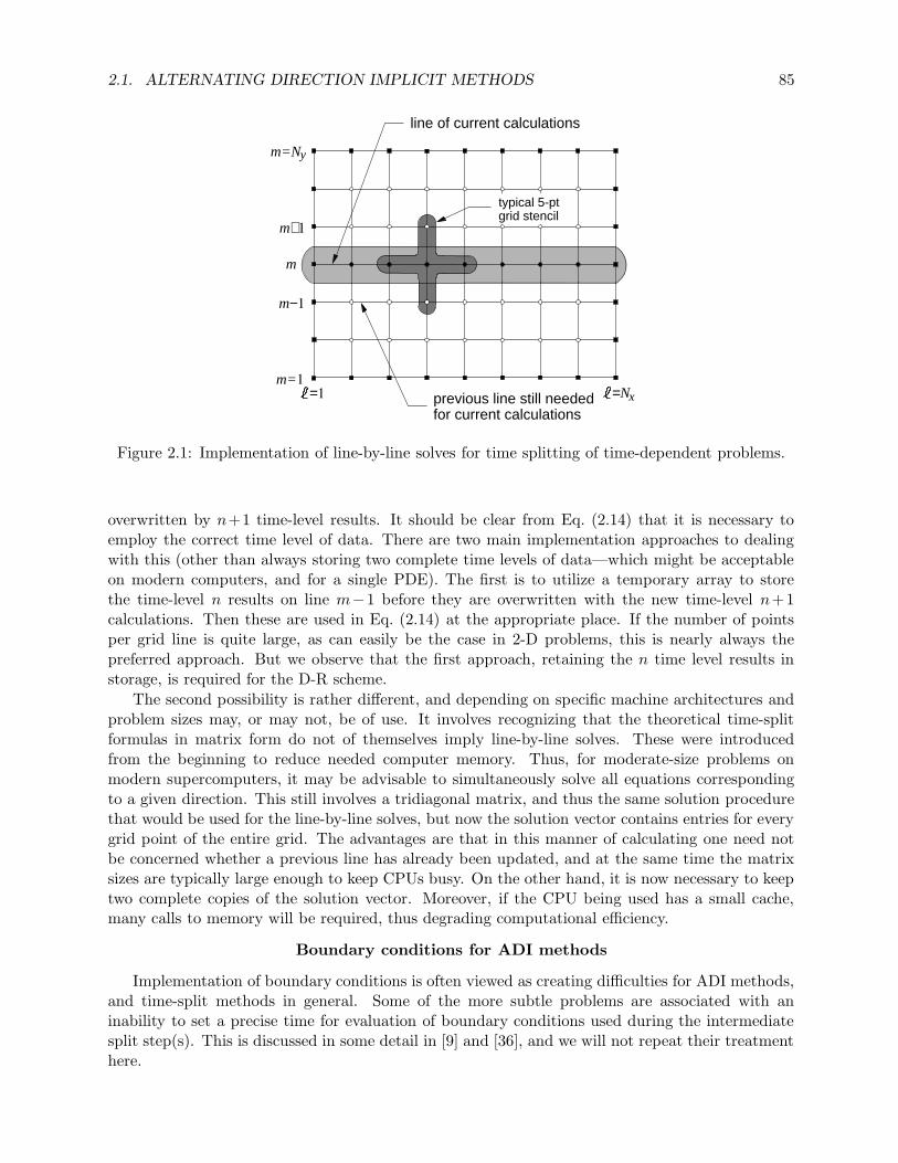
2.1. ALTERNATING DIRECTION IMPLICIT METHODS 85
previous line still neededfor current calculations
line of current calculations
typical 5-ptgrid stencil
m
m−1
m+1
m=1
m=N y
=1 =Nx
Figure 2.1: Implementation of line-by-line solves for time splitting of time-dependent problems.
overwritten by n+1 time-level results. It should be clear from Eq. (2.14) that it is necessary toemploy the correct time level of data. There are two main implementation approaches to dealingwith this (other than always storing two complete time levels of data—which might be acceptableon modern computers, and for a single PDE). The first is to utilize a temporary array to storethe time-level n results on line m−1 before they are overwritten with the new time-level n+1calculations. Then these are used in Eq. (2.14) at the appropriate place. If the number of pointsper grid line is quite large, as can easily be the case in 2-D problems, this is nearly always thepreferred approach. But we observe that the first approach, retaining the n time level results instorage, is required for the D-R scheme.
The second possibility is rather different, and depending on specific machine architectures andproblem sizes may, or may not, be of use. It involves recognizing that the theoretical time-splitformulas in matrix form do not of themselves imply line-by-line solves. These were introducedfrom the beginning to reduce needed computer memory. Thus, for moderate-size problems onmodern supercomputers, it may be advisable to simultaneously solve all equations correspondingto a given direction. This still involves a tridiagonal matrix, and thus the same solution procedurethat would be used for the line-by-line solves, but now the solution vector contains entries for everygrid point of the entire grid. The advantages are that in this manner of calculating one need notbe concerned whether a previous line has already been updated, and at the same time the matrixsizes are typically large enough to keep CPUs busy. On the other hand, it is now necessary to keeptwo complete copies of the solution vector. Moreover, if the CPU being used has a small cache,many calls to memory will be required, thus degrading computational efficiency.
Boundary conditions for ADI methods
Implementation of boundary conditions is often viewed as creating difficulties for ADI methods,and time-split methods in general. Some of the more subtle problems are associated with aninability to set a precise time for evaluation of boundary conditions used during the intermediatesplit step(s). This is discussed in some detail in [9] and [36], and we will not repeat their treatmenthere.
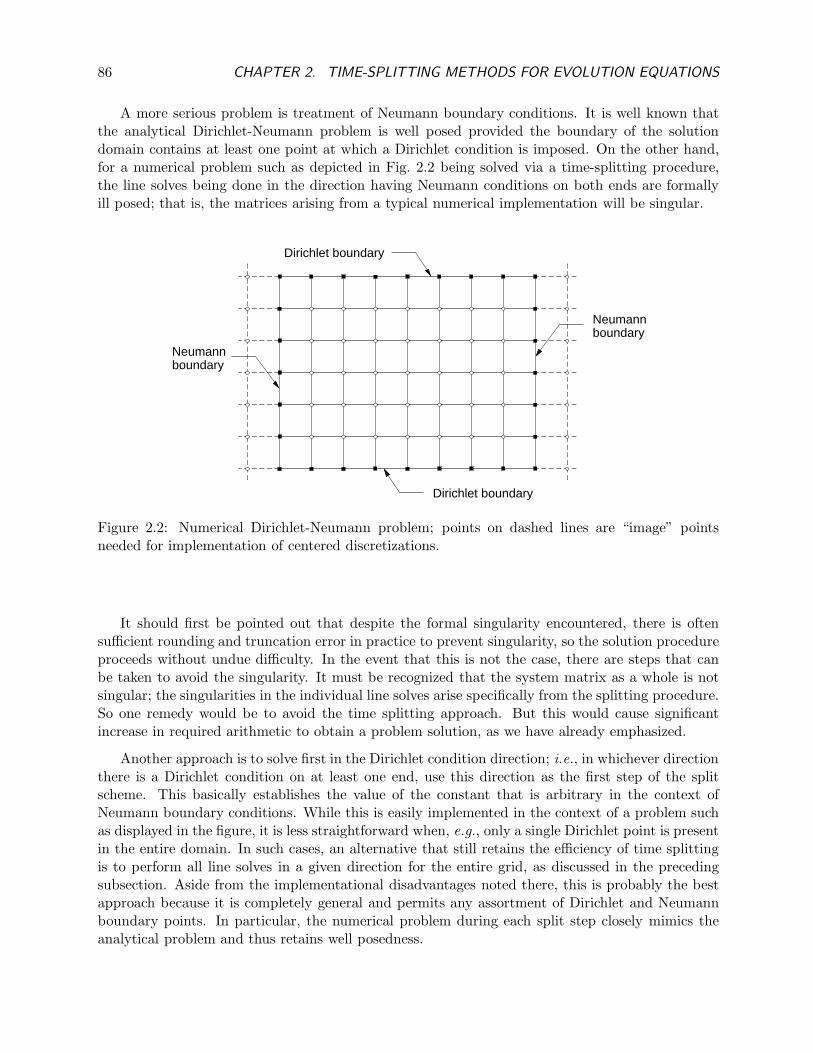
86 CHAPTER 2. TIME-SPLITTING METHODS FOR EVOLUTION EQUATIONS
A more serious problem is treatment of Neumann boundary conditions. It is well known thatthe analytical Dirichlet-Neumann problem is well posed provided the boundary of the solutiondomain contains at least one point at which a Dirichlet condition is imposed. On the other hand,for a numerical problem such as depicted in Fig. 2.2 being solved via a time-splitting procedure,the line solves being done in the direction having Neumann conditions on both ends are formallyill posed; that is, the matrices arising from a typical numerical implementation will be singular.
Dirichlet boundary
Dirichlet boundary
Neumannboundary
Neumannboundary
Figure 2.2: Numerical Dirichlet-Neumann problem; points on dashed lines are “image” pointsneeded for implementation of centered discretizations.
It should first be pointed out that despite the formal singularity encountered, there is oftensufficient rounding and truncation error in practice to prevent singularity, so the solution procedureproceeds without undue difficulty. In the event that this is not the case, there are steps that canbe taken to avoid the singularity. It must be recognized that the system matrix as a whole is notsingular; the singularities in the individual line solves arise specifically from the splitting procedure.So one remedy would be to avoid the time splitting approach. But this would cause significantincrease in required arithmetic to obtain a problem solution, as we have already emphasized.
Another approach is to solve first in the Dirichlet condition direction; i.e., in whichever directionthere is a Dirichlet condition on at least one end, use this direction as the first step of the splitscheme. This basically establishes the value of the constant that is arbitrary in the context ofNeumann boundary conditions. While this is easily implemented in the context of a problem suchas displayed in the figure, it is less straightforward when, e.g., only a single Dirichlet point is presentin the entire domain. In such cases, an alternative that still retains the efficiency of time splittingis to perform all line solves in a given direction for the entire grid, as discussed in the precedingsubsection. Aside from the implementational disadvantages noted there, this is probably the bestapproach because it is completely general and permits any assortment of Dirichlet and Neumannboundary points. In particular, the numerical problem during each split step closely mimics theanalytical problem and thus retains well posedness.
2.2. LOCALLY ONE-DIMENSIONAL METHODS 87
2.2 Locally One-Dimensional Methods
Locally one-dimensional (LOD) methods were first introduced by numerical analysts of the formerSoviet Union and are treated in detail by Yanenko [40] with the often-used terminology “method offractional steps.” A fairly complete, but condensed, treatment is provide by Mitchell and Griffiths[9], and we will to some extent follow that herein. Construction of LOD methods differs fromwhat we have just studied for ADI techniques in that the differential equations are split first(usually, but not always, directionally), and the result is then discretized by standard methods.This eliminates the factorization step altogether, so it is a simpler procedure that is more readilyanalyzed. Moreover, it is typically also somewhat easier to implement because each split step isoften completely one dimensional. (Recall that in the P-R ADI procedure, the individual solvesare 1D, but the right-hand side of the equations contains information from the opposite direction.)On the other hand, because the differential operators have been split, it is difficult to maintain thesame order of accuracy with LOD methods as achieved by the unsplit scheme unless the originalprocedure is only first-order accurate.
To demonstrate the LOD approach, we will again consider Eq. (2.1a):
ut = ∆u + f(x, y, t) .
As noted above, we begin by splitting the differential equation. In LOD methods this is done alongspatial directions, and in the present case it results in
1
2ut = uxx +
1
2f(x, y, t) , (2.15a)
1
2ut = uyy +
1
2f(x, y, t) . (2.15b)
Observe that the sum of these two equations is the original PDE, and this immediately suggeststhe approach to be applied in 3D.
We can now apply the Crank-Nicolson method (or any other desired technique) to each equationseparately. It is standard in 2D to perform each such discretization over a one-half time step; thusthe discrete formulas are
(I − k
2D2
0,x
)un+1/2 =
(I +
k
2D2
0,x
)un +
k
4
(fn+1/2 + fn
), (2.16a)
(I − k
2D2
0,y
)un+1 =
(I +
k
2D2
0,y
)un+1/2 +
k
4
(fn+1 + fn+1/2
). (2.16b)
It is important to remark here that neither (2.16a) nor (2.16b) is consistent with the original PDE.Nevertheless, as we will demonstrate in what follows, when the equations are used as indicated, theresult is consistent, and first-order accurate in time.
As usual, we write these in the simplified notation(
I − k
2A
)un+1/2 =
(I +
k
2A
)un +
k
4
(fn+1/2 + fn
), (2.17a)
(I − k
2B
)un+1 =
(I +
k
2B
)un+1/2 +
k
4
(fn+1 + fn+1/2
), (2.17b)
and then attempt to recover the unsplit discrete equations, which in the present case would bethe Crank-Nicolson method applied to the 2-D heat equation, namely Eq. (2.2). We begin bysolving Eq. (2.17a) for un+1/2 and substituting this result into Eq. (2.17b). After multiplication by(I − k
2A), this results in
88 CHAPTER 2. TIME-SPLITTING METHODS FOR EVOLUTION EQUATIONS
(I − k
2A
)(I − k
2B
)un+1 =
(I − k
2A
)(I +
k
2B
)(I − k
2A
)−1[(I +
k
2A
)un +
k
4
(fn+1/2 + fn
)]
+k
4
(I − k
2A
)(fn+1 + fn+1/2
). (2.18)
It is easy to see that if A and B commute, then we can write this as
(I − k
2A
)(I − k
2B
)un+1 =
(I +
k
2A
)(I +
k
2B
)un +
k
4
(I +
k
2B
)(fn+1/2 + fn
)
+k
4
(I − k
2A
)(fn+1 + fn+1/2
)
=
(I +
k
2A
)(I +
k
2B
)un +
k
4
(fn+1 + 2fn+1/2 + fn
)
+k2
8
[B(fn+1/2 + fn
)− A
(fn+1 + fn+1/2
)]
=
(I +
k
2A
)(I +
k
2B
)un +
k
2
(fn+1 + fn
)
+k2
8
[B(fn+1/2 + fn
)− A
(fn+1 + fn+1/2
)]+ O(k3) .
Note that the O(k3) term arises from what is essentially an O(k2)-accurate filtering of fn+1/2 inthe second step, above, and viewing this as arising from midpoint integration of the result. Inparticular, this is within O(k3) of the trapezoidal integration shown in the last step, and which isneeded to coincide with the Crank-Nicolson procedure of the unsplit scheme.
It is clear that even if A and B commute, unless f ≡ 0, the error due to splitting will be O(k2)locally. We have not considered the equivalent factorization error, which from the form of theequations is obviously still present even though no formal factorization was employed, because ifu ∈ C1 this is an O(k3) error just as was true for P-R ADI, and is thus higher order.
It is worthwhile to consider the case f ≡ 0, but for AB 6= BA to examine the nature of thesplitting error, and from this propose a way to remove it. In Eq. (2.18) we have
(I − k
2A
)(I +
k
2B
)= I − k
2(A − B) − k2
4AB ,
and (I +
k
2B
)(I − k
2A
)= I − k
2(A − B) − k2
4BA ;
hence, (I − k
2A
)(I +
k
2B
)=
(I +
k
2B
)(I − k
2A
)− k2
4(AB − BA) .
Thus, in the homogeneous case (2.18) can be written as
(I − k
2A
)(I − k
2B
)un+1 =
(I +
k
2B
)(I +
k
2A
)un − k2
4(AB − BA)
(I − k
2A
)−1(I +
k
2A
)un .

2.2. LOCALLY ONE-DIMENSIONAL METHODS 89
We also have, similar to relations found earlier,
(I +
k
2B
)(I +
k
2A
)=
(I +
k
2A
)(I +
k
2B
)− k2
4(AB − BA) ,
so the above becomes(
I − k
2A
)(I − k
2B
)un+1 =
(I +
k
2A
)(I +
k
2B
)un
−k2
4(AB − BA)
[I +
(I − k
2A
)−1(I +
k
2A
)]un, (2.19)
which clearly demonstrates the O(k2) error in the absence of commutativity of A and B.Finally, we note that (
I − k
2A
)−1
=
(I +
k
2A
)+ O(k2) ,
as is easily checked; thus, the O(k2) term can be expressed as
k2
4(AB − BA)
[I +
(I +
k
2A
)2]
un + O(k3) ,
or simplyk2
2(AB − BA)un + O(k3) .
We next observe that, at least in 2D, there is a straightforward way to recover full second-orderaccuracy with LOD methods. It is simply to perform each time step twice, switching the directionthat is done first between the two calculations, and then averaging the results. In the homogeneouscase it is easily checked that this results in cancellation of the commutator AB−BA. Moreover, onmodern parallel computers the run times are essentially the same as for doing the time step oncesince the calculations are completely independent and can be done in parallel. In principle, sucha treatment can be extended to nonhomogeneous problems, and to three space dimensions; but ineither of these cases it is not so direct, and especially in the latter becomes rather inefficient. Weleave further details of this sort to the reader, and to references such as [9].
There is one final observation we should make regarding LOD procedures. Unless first-ordertemporal accuracy is acceptable, they probably should not be used in the spatial time-splittingmode considered here. But these methods provide simple models of general operator-splittingmethods that are in very wide use in many contexts, especially in CFD, and the analysis tools wehave presented here apply in these cases as well. Indeed, one of the main approaches to solvingthe incompressible Navier–Stokes equations is a class of techniques known as projection methods.Although these differ considerably from one particular method to the next, they are all based onthe notion of operator splitting implemented (conceptually) as follows.
We can write the momentum equations of incompressible flow as
U t + U ·∇U = −∇P +1
Re∆U ,
where U ≡ (u, v, w)T is the velocity vector, and P ≡ p/ρ is “kinematic” pressure; p is the usualhydrodynamic pressure, and ρ is (constant) density. Pressure-velocity coupling is a rather difficultaspect of solving these equations together with satisfaction of the divergence-free constraint ∇·U =

90 CHAPTER 2. TIME-SPLITTING METHODS FOR EVOLUTION EQUATIONS
0. But this can be accomplished quite efficiently through an operator-splitting procedure analogousto what we have studied in this section. Namely, we first solve the momentum equations withoutthe pressure gradient term, written as
U t + U ·∇U =1
Re∆U .
This is relatively easy to accomplish because this system contains only mild nonlinearities (seeChap. 3 of these notes for efficient ways to treat these) and is otherwise just a weakly-coupledparabolic system. After this has been done, the equation
U t = −∇P
is solved. This is not usually carried out in the direct manner implied here, and we will not elaborateon the details. The main point is that an operator splitting has been employed to significantlysimplify an otherwise fairly difficult problem.
2.3 General Douglas-Gunn Procedures
We will begin presentation of the Douglas-Gunn [41] time splitting methods in the context ofthe straightforward two-level scheme that is widely used for parabolic PDEs. We will provide aquite detailed treatment of this method, including thorough analysis of truncation error and abrief indication of problems posed by the presence of mixed derivatives in the differential operator.We will then consider the more general multi-level Douglas-Gunn schemes that are applicable tosecond-order hyperbolic problems and in the development of more elaborate techniques for parabolicequations. We will close the section with some discussion concerning details of implementation,including differences from that of ADI and LOD, and especially boundary condition treatment.
One aspect of the D-G methods that will be apparent for both two-level and multi-level versionsis the basic approach to their derivation. One can think of the steps required to construct a D-Gscheme as being exactly the reverse of those employed for LOD; namely, we first discretize thePDE, and then we split the result. There is no formal factorization as found in the ADI methods,but as we have already seen for LOD (for which this is also true), there can be a factorization error.
2.3.1 D-G methods for two-level difference equations
We begin by noting that the problems to which the D-G methods can be applied are quite generaland may be expressed as
∂u
∂t− Lu = f(x, t) with x ∈ Ω ⊂ R
p , t ∈ (t0, tf ] . (2.20)
Initial conditions
u(x, t0) = u0(x) ,
and boundary conditions
BΩu = g(x, t) x ∈ ∂Ω ,
are required to formulate a well-posed initial boundary value problem. In (2.20) L is a generalsecond-order linear elliptic operator, and BΩ is any combination of (linear) boundary operatorsleading to a well-posed problem. It will be formally assumed that u(x, t) ∈ C 2(Ω)×C1((t0, tf ]),but in many situations it is sufficient to instead have u(x, t) ∈ H 2(Ω)×L1((t0, tf ]).
2.3. GENERAL DOUGLAS-GUNN PROCEDURES 91
Any two-level difference approximation of Eq. (2.20) can be cast in the form(I + An+1
)un+1 + Bnun = sn , (2.21)
where it is assumed that all discrete boundary data are contained in the matrices A and B, aswell as in sn, as appropriate. We also note that the matrices A and B may be time dependent,as indicated by the notation; in particular, the matrix A will always represent advanced time leveldifference equation coefficients and correpondingly, B will denote previous time-level information.Hence, with this understood, we will often suppress the superscripts to simplify notation. Finally,we remark that the grid function sn is taken to be known for all time, and in many cases (e.g., theCrank-Nicolson method) it will actually contain information from the advanced time level.
Construction of the basic D-G method
In the treatment of Eq. (2.21) to be provided here we will closely follow the paper by Douglasand Gunn [41], but with occasional changes in notation. We recognize that the next step afterobtaining the above discretization is splitting. To accomplish this we begin by noting that thematrix A can be written as a sum of matrices,
A =
q∑
i=1
Ai .
Typically, but not always, q = p, and each Ai is associated with a specific spatial direction. (Itis worthwhile to recall that the steady-state form of P-R ADI was formulated in an analogousfashion.) Also, let v(1), v(2), . . . , v(q−1) denote intermediate estimates of un+1, with v(q) = un+1.
The Douglas-Gunn procedure for determining each of the v(i)s, and hence un+1, is the following.For each i = 1, 2, . . . , q solve the system of equations
(I + An+1
i
)v(i) +
i−1∑
j=1
An+1j v(j) +
q∑
j=i+1
An+1j un + Bnun = sn , (2.22)
where each An+1i is a N×N matrix that is usually tridiagonal. We have here included the time-level
superscripts for emphasis.Now observe that the first summation in (2.22) contains intermediate solution vectors that all
have been calculated during previous substeps of the current time step, while the second summationcontains portions of the split matrix from beyond the current substep—but operating on resultsfrom the preceding (and thus, known) time step. (Note that this resembles the structure of Gauss-Seidel iteration; viz., use new information in succeeding substeps as soon as it is generated.)
It should be clear from (2.22) that there is a considerable amount of arithmetic needed toevaluate the q equations of this form unless extra storage is used to avoid recalculations. But thiscan be reduced significantly by the following rearrangement. If we write (2.22) for the i − 1th
substep we obtain (with time indexing suppressed)
(I + Ai−1) v(i−1) +
i−2∑
j=1
Ajv(j) +
q∑
j=i
Ajun + Bun = sn .
Then subtracting this from Eq. (2.22) yields
(I + Ai) v(i) − (I + Ai−1) v(i−1) +i−1∑
j=1
Ajv(j) −
i−2∑
j=1
Ajv(j) +
q∑
j=i+1
Ajun −
q∑
j=i
Ajun = 0 ,
92 CHAPTER 2. TIME-SPLITTING METHODS FOR EVOLUTION EQUATIONS
or(I + Ai) v(i) − v(i−1) −Aiu
n = 0 .
It is clear from this that from the standpoint of computational efficiency the v (i)s should becalculated from the following formulas:
(I + A1) v(1) +
q∑
j=2
Ajun + Bun = sn , (2.23a)
(I + Ai) v(i) − v(i−1) −Aiun = 0 i = 2, 3, . . . , q , (2.23b)
with un+1 = v(q). We observe that these equations are of precisely the same form (up to notation)as those given earlier for Douglas-Rachford ADI. Thus, we now see how such a time splitting canbe produced systematically from first principles.
In the following subsections we will demonstrate several important features of this procedure inthe context of the 2-D heat equation considered earlier for both ADI and LOD methods. We willfirst show that each of the individual split steps of D-G schemes are consistent with the PDE; wethen show that the order of accuracy of the original unsplit discretization is preserved after splitting.Finally, we will provide results concerning stability and state a general theorem associated with allof these features.
Consistency of individual split steps
It is worthwhile at this point to consider a specific example of applying the preceding formulas.For sake of comparison we will again consider the 2-D transient heat equation already treated viaboth ADI and LOD methods. Thus, in the general notation of Eq. (2.20) L = ∆, BΩ = I, andwe again have Eq. (2.1a). As before, we will apply a Crank-Nicolson discretization leading to Eq.(2.2), repeated here as:
[I − k
2
(D2
0,x + D20,y
)]un+1
`,m =
[I +
k
2
(D2
0,x + D20,y
)]un
`,m +k
2
(fn+1
`,m + fn`,m
). (2.24)
In the notation of the general two-level discrete scheme, Eq. (2.21), we see that
A ≡ −k
2
(D2
0,x + D20,y
),
B ≡[I +
k
2
(D2
0,x + D20,y
)],
sn ≡ k
2
(fn+1 + fn
).
Furthermore, it is clear that we can set
A = A1 + A2 = −k
2A1 −
k
2A2
with A1 ≡ D20,x and A2 ≡ D2
0,y. In this simple case, q = 2, and we can write Eq. (2.22) as
(I − k
2A1
)v(1) =
[I +
k
2(A1 + A2)
]un +
k
2A2u
n +k
2
(fn+1 + fn
), (2.25a)
(I − k
2A2
)v(2) =
[I +
k
2(A1 + A2)
]un +
k
2A1v
(1) +k
2
(fn+1 + fn
), (2.25b)
2.3. GENERAL DOUGLAS-GUNN PROCEDURES 93
for the two split steps.We will now show that both of these individual split steps is consistent with the PDE with the
v(i)s viewed as approximations to un+1. Note that this is in sharp contrast to the situation for LODmethods treated earlier. It should be clear that if v(1) is a consistent approximation to un+1, thenthe second split step is consistent since in this case it is analogous to the unsplit Crank-Nicolsonscheme. Hence, we need only demonstrate consistency of Eq. (2.25a).
We begin by expanding v(1) in a Taylor series under the assumption that it is an approximationto un+1, as needed. Thus,
v(1) = un + kunt +
k2
2un
tt + · · · .
Substitution of this into (2.25a) results in(
I − k
2A1
)un =
[I +
k
2(A1 + A2)
]un +
k
2A2u
n +k
2
(fn+1 + fn
)
−(
I − k
2A1
)[kun
t +k2
2un
tt + · · ·]
,
and rearrangement leads to
kunt = k (A1 + A2)un +
k
2
(fn+1 + fn
)+ O(k2) .
Also note thatfn+1 + fn = 2fn + O(k) ,
and from the definitions of the Ais, A1 + A2 = ∆ + O(h2). Thus, division by k leaves
unt = ∆un + fn + O(k + h2) .
Hence, we have shown that the first split step of the Douglas-Gunn formalism is consistent withthe original PDE, and alone it is first-order accurate in time. Moreover, we have already arguedthat consistency of the first split step implies consistency of the second in this case. A majorconsequence of this feature of the D-G schemes is that it removes the question of when in time toevaluate boundary conditions for the split-step time levels. In particular, we have demonstratedthat the the intermediate results are consistent approximations to the n + 1th time level results, soboundary conditions should be implemented accordingly.
Accuracy of the complete method
We next show that the two consistent steps of the D-G procedure, when combined, lead torecovery of full second-order accuracy of the original discretization. We begin by writing theequivalent form given in an earlier subsection, namely Eqs. (2.23), rearranged as
(I − k
2A1
)v(1) =
[I +
k
2(A1 + 2A2)
]un +
k
2
(fn+1 + fn
), (2.26a)
(I − k
2A2
)un+1 = v(1) − k
2A2u
n . (2.26b)
As we have done previously, we solve the first of these for v(1),
v(1) =
(I − k
2A1
)−1 [I +
k
2(A1 + 2A2)
]un +
k
2
(I − k
2A1
)−1 (fn+1 + fn
),

94 CHAPTER 2. TIME-SPLITTING METHODS FOR EVOLUTION EQUATIONS
and substitute this result into the second equation. This yields
(I − k
2A2
)un+1 =
(I − k
2A1
)−1[I +
k
2(A1 + 2A2)
]un +
k
2
(fn+1 + fn
)− k
2A2u
n .
Now multiply this result by(I − k
2A1
)to obtain the required form on the left-hand side:
(I − k
2A1
)(I − k
2A2
)un+1 =
[I +
k
2(A1 + 2A2)
]un +
k
2
(fn+1 + fn
)− k
2
(I − k
2A1
)A2u
n ,
or(
I − k
2A1
)(I − k
2A2
)un+1 =
[I +
k
2(A1 + A2)
]un +
k
2
(fn+1 + fn
)+
k2
4A1A2u
n .
Now recall that (I − k
2A1
)(I − k
2A2
)=
[I − k
2(A1 + A2)
]+
k2
4A1A2 ,
which leads to the desired result[I − k
2(A1 + A2)
]un+1 =
[I +
k
2(A1 + A2)
]un +
k
2
(fn+1 + fn
)− k2
4A1A2(u
n+1 − un) . (2.27)
We see from this that if u ∈ C1 we have recovered the unsplit Crank-Nicolson scheme to withinO(k3) local accuracy, and this has been done for a general nonhomogeneous problem without anyrequirement of commutativity of the matrices A1 and A2. We also note that this is still true forproblems with time-dependent coefficients (a major problem for many time-split methods), theproof of which is left as an exercise for the reader.
Stability
We now briefly consider stability of the Douglas-Gunn time-splitting procedure. To do this itis convenient to introduce the so-called δ-form of the method, as done in [41]. We also remark thatthis form is now widely used in computational algorithms and is the most efficient of the forms wehave considered.
We start by observing that Eq. (2.23b) can be written as
(I + Ai)(v(i) − un
)= v(i−1) − un
by subtracting un from both sides. Now define
δv(i) ≡ v(i) − un
so that(I + Ai) δv(i) = δv(i−1) ∀ i = 2, . . . , q . (2.28)
Similarly, by subtracting (I + A1)un from both sides of (2.23a), we obtain
(I + A1) δv(1) = sn − (I + A)un − Bun . (2.29)
We will use this to show that the split scheme, viewed in complete generality (in contrast to thespecific example problem treated above), is equivalent to the original unsplit difference equations
2.3. GENERAL DOUGLAS-GUNN PROCEDURES 95
plus a small perturbation. Then, for linear problems, if the unsplit scheme is stable so must be thesplit method.
From (2.28) we work backwards starting with i = q to obtain
δv(q−1) = (I + Aq)δv(q)
δv(q−2) = (I + Aq−1)δv(q−1) = (I + Aq−1)(I + Aq)δv
(q)
...
δv(1) = (I + A2)δv(2) = · · · =
q∏
j=2
(I + Aj)
δv(q) ,
or
v(1) − un =
q∏
j=2
(I + Aj)
(un+1 − un) .
Substitution of this into Eq. (2.29) yields
q∏
j=1
(I + Aj)
(un+1 − un) + (I + A)un + Bun = sn . (2.30)
Now let σ be the multi-index (i1, i2, . . . , im) with i1 < i2 < · · · < im, with 2 ≤ m ≤ q, and|σ| = i1 + · · · + im. Then expanding the product in Eq. (2.30) leads to
(I + A)un+1 + Bun +∑
2≤|σ|≤q
Aσ(un+1 − un) = sn , (2.31)
where
Aσ =
m∏
`=1
Ai` .
We can observe from this that, first Eq. (2.31) is the perturbation of the original difference equation,Eq. (2.21), mentioned above. Second, if u ∈ C1 the factor un+1 − un is O(k) and third, from thedefinition of the matrices Ai and Aσ, the Aσs must be no more than O(k2). Hence, the perturbationis, in general, of the same order as the splitting error demonstrated for the model heat equationproblem treated in detail above; so for a linear problem this would not grow in time if the unsplitscheme is stable.
In Douglas and Gunn [41] various results concerning consistency, accuracy and stability areproven as separate theorems. We collect that information in the following theorem. The foregoinganalyses we have presented here have not been done with sufficient rigor to constitute a proof ofthe theorem. On the other hand, they at least suggest that the theorem can be proven.
Theorem 2.1 (Douglas & Gunn Time Splitting) Suppose that a consistent and stable unsplitapproximation has been provided for Eq. (2.20), and the corresponding split scheme has been re-composed as Eq. (2.31). Then the following hold:
i) Eq. (2.31) is consistent in the norm ‖ · ‖ provided
limh,k→0
maxt0≤nk≤tf
∥∥∥∥∥∥k−1
∑
2≤|σ|≤q
Aσ(un+1 − un)
∥∥∥∥∥∥= 0 .

96 CHAPTER 2. TIME-SPLITTING METHODS FOR EVOLUTION EQUATIONS
ii) Eq. (2.31) is stable provided the operators A1,A2, . . . ,Aq and B have the following properties:
(a) Ai is nonnegative definite ∀ i = 1, . . . , q;
(b) B is Hermitian;
(c) A1,A2, . . . ,Aq, B commute.
iii) Under the above hypotheses, and in addition assuming that u ∈ C∞(Ω), the formal globalaccuracy of the split scheme is the same as that of the original unsplit scheme.
There are several things to note regarding this theorem. First, commutativity is not necessaryfor maintaining order of accuracy, as implied by the theorem statement, at least in the contextof the Crank-Nicolson scheme. The same may also be true for stability; however, it should benoted that this is somewhat less easily tested because the specific types of problems that lead tononcommutativity can also lead to instabilities of the unsplit Crank-Nicolson method—namely,time-dependent coefficients in the differential operators. Finally, with regard to accuracy, therequirement of C∞ solutions was a standard one at the time the original work by Douglas andGunn was done. It is recognized in modern numerical analysis that much less than this is needed.In particular, it is usually sufficient to have u∈Hm(Ω) where m is the order of the derivative in theleading term of the truncation error expansion; i.e., this leading term is in L2(Ω) and is thereforebounded almost everywhere, and has finite energy, in Ω.
There is one additional item associated with this two-level splitting procedure that we willconsider briefly. It is treatment of problems containing mixed derivatives. We refer the readerto Mitchell and Griffiths [9] for a thorough analysis of this problem. Here, we first point outthat it is a problem that seems to have to good solution in the context of time split schemes.Possibly the most successful attempts are embodied in the family of methods proposed by Beamand Warming [42] in the early 1980s. In the context of the splitting procedures just described, apossible alternative is to perform additional split steps to separately treat the mixed derivative,analogous to the operator splitting already treated in conjunction with LOD methods. In twospace dimensions if one considers difference operators defined along diagonal lines of the grid assuggested in [41], it is easily checked that two such operators are needed to construct the usualcentered approximation to a second mixed derivative. In this case, one can take q = 4 and proceedjust as we have already done. Of course this entails essentially double the arithmetic per timestep, and it requires much more complicated data structures for the diagonal direction solves. Thesituation is far more complcated in 3D; thus, this does not seem to be a very practical approachto this problem. We mention, in passing, that for nonlinear problems requiring iteration at eachtime step, simply lagging the mixed derivative and evaluating it with currently-known data usuallyworks quite well. It does not generally slow convergence of the nonlinear iterations, and it typicallyhas little effect on stability (which will already have been influenced by the nonlinearities).
2.3.2 D-G methods for multi-level difference equations
Following Douglas and Gunn [41] we define a (M+2)-level difference equation approximating atime-dependent partial differential equation by
(I + A)un+1 +
M∑
m=0
Bmun−m = sn , M ≤ n , (2.32)
where u0, u1, . . . , un are assumed to have been specified. Clearly, in general, such methods havethe same disadvantages as do multi-step schemes for ODEs: namely, they are not generally self
2.3. GENERAL DOUGLAS-GUNN PROCEDURES 97
starting, and they require considerably more storage, especially in the PDE case. But in addition,stability is more difficult to analyze, and subtle errors can occur due to short periods of instabilityfollowed by return of stable behavior before a numerical solution actually diverges to infinity. Onthe other hand, an advantage in the PDE case is that such methods can be used for both parabolicand higher-order hyperbolic problems (e.g., the second-order wave equation).
Basic construction
We again assume A to be decomposable as∑
i Ai. Also, we let ϕm, m = 0, 1, . . . ,M , be constantssuch that
M∑
m=0
ϕm = 1 ,
and define
un+1∗ ≡M∑
m=0
ϕmun−m .
Thus, if the ϕms are chosen properly, un+1∗ provides a prediction, via extrapolation, of un+1.We can now form the split version of Eq. (2.32) in a way that is analogous to the splitting of
two-level methods given in the preceding section:
(I + Ai)v(i) +
i−1∑
j=1
Ajv(j) +
q∑
j=i+1
Ajun+1∗ +
M∑
m=0
Bmun−m = sn , i = 1, 2, . . . , q . (2.33)
As was true for the two-level schemes treated earlier, this equation can be simplified and mademore computationally efficient, analogous to Eqs. (2.23); in fact, even a δ-form can be constructed.We leave investigation of this to the interested reader and consider the following example whilemaintaining the form given in (2.33).
Example problem: the 3-D wave equation
We, as yet, have not treated either 3-D problems, or hyperbolic problems. We will use thismulti-level scheme to remedy this omission. We consider the initial boundary value problem forthe nonhomogeneous 3-D wave equation expressed as
utt − (uxx + uyy + uzz) = f(x, y, z, t) on Ω×(t0, tf ) (2.34)
with Ω ⊂ R3assumed to be a rectangle. Initial data are given as
u(x, y, z, t0) = u0(x, y, z)
ut(x, y, z, t0) = ut,0(x, y, z) ,
and boundary conditions are prescribed as
u(x, y, z, t) = g(x, y, z, t) on ∂Ω .
If we were to formulate (2.34) as a first-order system we could directly apply the Crank-Nicolsonprocedure to obtain a two-level scheme and proceed as we have done in the preceding section. Here,we will employ a somewhat ad hoc procedure not very different from what is often done for the

98 CHAPTER 2. TIME-SPLITTING METHODS FOR EVOLUTION EQUATIONS
1-D wave equation. Namely, we will use centered-difference discretizations in both space and time,but we will average the spatial parts over all three time levels used in the temporal discretizationin order to maintain full second-order accuracy. Thus, we can express (2.34) in discrete form as
un−1−2un+un+1 =k2
3
[(D2
0,x + D20,y + D2
0,z
) (un−1 + un + un+1
)+(fn−1 + fn + fn+1
)], (2.35)
where, as often done, we have suppressed grid-point indexing. If we now make our usual identifica-tions between difference operators and their corresponding matrices of coefficients, viz., D2
0,x ≡ A1,
D20,y ≡ A2 and D2
0,z ≡ A3 we can write the above as
[I − k2
3(A1 + A2 + A3)
]un+1 −
[2I +
k2
3(A1 + A2 + A3)
]un
+
[I − k2
3(A1 + A2 + A3)
]un−1 =
k2
3
(fn−1 + fn + fn+1
). (2.36)
Clearly, M = 1 in this case, and we can identify the matrices appearing in Eq. (2.32) as
A ≡ −k2
3(A1 + A2 + A3) ,
B0 ≡ −[2I +
k2
3(A1 + A2 + A3)
],
B1 ≡[I − k2
3(A1 + A2 + A3)
],
sn ≡ k2
3
(fn−1 + fn + fn+1
).
Thus, we can express (2.36) as
(I + A)un+1 + B0un + B1u
n−1 = sn . (2.37)
We now split the matrix A in a manner analogous to what was done in the two-level case:A = A1 + A2 + A3 with obvious definitions for the Ais. Then the directionally-split equations are
(I + A1)v(1) +
0∑
j=1
Ajv(j) +
3∑
j=2
Ajun+1∗ +
1∑
m=0
Bmun−m = sn
(I + A2)v(2) +
1∑
j=1
Ajv(j) +
3∑
j=3
Ajun+1∗ +
1∑
m=0
Bmun−m = sn
(I + A3)v(3) +
2∑
j=1
Ajv(j) +
3∑
j=4
Ajun+1∗ +
1∑
m=0
Bmun−m = sn .
It is to be noted that the first sum in the first of these equations, and the second sum in the third,are vacuous. Thus, we can express these as
(I − k2
3A1
)v(1) = sn +
k2
3(A2 + A3)u
n+1∗ +
[2I +
k2
3(A1 + A2 + A3)
]un
−[I − k2
3(A1 + A2 + A3)
]un−1 ,
(2.38a)
2.3. GENERAL DOUGLAS-GUNN PROCEDURES 99
(I − k2
3A2
)v(2) = sn +
k2
3
(A1v
(1) + A3un+1∗
)+
[2I +
k2
3(A1 + A2 + A3)
]un
−[I − k2
3(A1 + A2 + A3)
]un−1 ,
(2.38b)
(I − k2
3A3
)un+1 = sn +
k2
3
(A1v
(1) + A2v(2))
+
[2I +
k2
3(A1 + A2 + A3)
]un
−[I − k2
3(A1 + A2 + A3)
]un−1 .
(2.38c)
Before proceeding further, we should make several observations regarding Eqs. (2.38). First, theimplicit part of each of these equations is tridiagonal, and is thus easily solved. Second, each stepof the split scheme is consistent with the original differential equation, implying straightforwardboundary condition implementation. Finally, stability properties of this method are not completelyknown. It is clear that a von Neumann analysis will provide only necessary conditions for stabilityin this case. The general theorems of [41] can be applied to infer stability, but these theorems aresomewhat weak.
In order to implement the above split scheme we must determine the ϕms to permit calculationof un+1∗ , and when n = 1 we must find u1. We choose the ϕms to correspond to a simple linearextrapolation in time; i.e., we set
un+1∗ = 2un − un−1.
Thus, ϕ0 = 2 and ϕ1 = −1. It is worth mentioning here that linear extrapolation is formallysecond-order accurate, so consistency of the individual steps is not harmed by this technique. Onthe other hand, extrapolation can be destabilizing, and its use must be examined for each individualcase.
In order to calculate u1 we recognize that at the first calculated level of the basic differenceequations we obtain u2, so a different formulation is needed for the first time step. We first notethat u0 and u0
t are given as initial data. We then assume that u is sufficiently smooth at the initialtime to permit expansion in a Taylor series as
u1 = u0 + k
(∂u
∂t
)0
+k2
2
(∂2u
∂t2
)0
+ O(k3) .
As already noted, the first two terms in the right-hand side of this expression are known; the thirdterm can be obtained from the differential equation. In particular,
(∂2u
∂t2
)0
= (uxx + uyy + uzz)0 + f .
Hence, u1 can be determined to within O(k3) since u0 is given throughout Ω. If u0 is prescribedin functional form, the required derivatives can be computed analytically; otherwise, they mustbe approximated using the same centered discretizations used throughout the remainder of theformulation. So the procedure is essentially self starting. This completes analysis of the waveequation example.
100 CHAPTER 2. TIME-SPLITTING METHODS FOR EVOLUTION EQUATIONS
Chapter 3
Various Miscellaneous Topics
In this chapter we will consider several topics that will allow us to generalize our preceding analyses.In previous chapters we have restricted attention to single, linear PDES with problems posed onrectangular domains. It is only the last of these restrictions that will not be treated in the presentchapter, and this will be studied in Chap. 4. Here, we will study the following topics: treatmentof nonlinear problems for PDEs, analysis of systems of differential equations and some advancedforms for discretizing special problems.
3.1 Nonlinear PDEs
There are numerous ways in which nonlinear problems can be treated, and this is despite thefact that the analytical theory is not nearly so well developed for nonlinear PDEs as it is for thelinear case. We will begin by giving the general form of the nonlinear PDEs to be studied, andwe follow this with several alternative approaches to treating them. In particular, we will brieflydiscuss the direct, explicit integration approach. We follow this with a short treatment of basicfixed-point iteration, or Picard iteration. Finally, we develop the Newton-Kantorovich procedurein considerable detail, analyzing both the basic form and the δ-form. We will describe how each ofthese approaches can be applied for either time-dependent or steady-state problems.
3.1.1 The general nonlinear problem to be considered
Here we will study fairly general nonlinear parabolic equations expressed in the form
ut = Lu + N(u, ux, uy) + f(x, y, t) (3.1)
on a domain Ω ⊂ Rd, d = 2, 3, together with appropriate boundary and initial data to comprise
a well-posed problem. Here, L is a linear operator (possibly null), and N is a general nonlinearfunctional of its arguments. We can write a general two-level discretization of this problem in theform
(I + A)un+1 + Bun = sn , (3.2)
which is identical to Eq. (2.21) except that now sn contains additional terms corresponding to N .
3.1.2 Explicit integration of nonlinear terms
The simplest approach to solving the numerical problem of (3.2) is to directly integrate the nonlin-earity N . This might be done in the context of splitting this term as in operator splitting described
101
102 CHAPTER 3. VARIOUS MISCELLANEOUS TOPICS
in the preceding chapter, or it could be done as part of the construction of (3.2). In either case, it isnot a highly-recommended approach because it can lead to instabilities in the difference equations.We will provide far more robust methods in what follows.
3.1.3 Picard iteration
The next level of complexity corresponds to basic fixed-point iteration, often termed Picard iterationespecially in the context of solving nonlinear differential equations. We begin by observing thatsince sn includes N(u), we should employ the formal notation
(I + A)un+1(m+1)+ Bun = sn(un+1(m)
) ,
or, in standard fixed-point form
un+1(m+1)= (I + A)−1
[N(un+1(m)
) − Bun − f]
. (3.3)
Clearly this is convergent only if (I + A)(−1)N(u) satisfies the Lipschitz condition
‖(I + A)−1N(u) − (I + A)−1N(v)‖ ≤ K‖u − v‖ , (3.4)
with K < 1 and u, v in a space of functions consistent with the operators L and N of Eq. (3.1). Itis generally difficult to satisfy inequality (3.4), and as a consequence it is usually preferable to usea form of Newton’s method.
3.1.4 The Newton-Kantorovich Procedure
The specific form of Newton’s method employed for solution of nonlinear PDEs varies with theinvestigator. Here, we will consider only the Newton-Kantorovich procedure (see, e.g., Kantorovichand Akilov [43]). The form of this that we shall employ herein is often termed quasilinearization(even though it is actually linearization and not quasilinearization), and some further details canbe found e.g., in Ames [44].
A basic approach
The simplest form of quasilinearization, from a conceptual standpoint is that introduced by Bellman(see Bellman and Kalaba [45]) in which each dependent variable, as well as its derivatives areviewed as independent variables in an Frechet-Taylor expansion of any nonlinear terms present inthe problem. For example, suppose N = N(u, ux, uy); then we linearize N as follows:
N(u, ux, uy) = N(u(0), u(0)x , u(0)
y ) +
(∂N
∂u
)(0)(u − u(0)
)+
(∂N
∂ux
)(0)(ux − u(0)
x
)
+
(∂N
∂uy
)(0)(uy − u(0)
y
)+ · · · , (3.5)
where the (0) superscript denotes an initial guess for u.At this point it is worthwhile to consider a specific temporal discretization so as to better see
how the Newton-Kantorovich iteration process must interact with the time-stepping algorithm. Weapply trapezoidal integration to Eq. (3.1) to obtain
un+1 = un +k
2
[L(un+1 + un
)+ N
(un+1, . . .
)+ N (un, . . .) + fn+1 + fn
]. (3.6)
3.1. NONLINEAR PDES 103
We observe that since un is already known, N(un, . . .) can be directly evaluated without using thelinearization given in Eq. (3.5). On the other hand, (3.5) must be used to approximate N(un+1, . . .).Substitution of this into Eq. (3.6) yields
un+1 = un +k
2
[L(un+1 + un
)+ N (0) +
(∂N
∂u
)(0)(u − u(0)
)+
(∂N
∂ux
)(0)(ux − u(0)
x
)
+
(∂N
∂uy
)(0)(uy − u(0)
y
)+ N(un, . . .) + fn+1 + fn
].
It should be noted that this equation is linear and can easily be cast in a form to which solutionalgorithms (such as time-splitting schemes) can be applied. In particular, we have
I − k
2
[L +
(∂N
∂u
)(0)
+
(∂N
∂ux
)(0) ∂
∂ux+
(∂N
∂uy
)(0) ∂
∂uy
]un+1 =
un +k
2
Lun + N (0) −
[(∂N
∂u
)(0)
u(0) +
(∂N
∂ux
)(0)
u(0)x +
(∂N
∂uy
)(0)
u(0)y
]+ fn+1 + fn
. (3.7)
We also note that if u(0) is set equal to un, then the first terms omitted from (3.5) are O(k2).As a consequence, Eq. (3.7) retains the formal (local) third-order accuracy of the original linearscheme—without iteration.
At this point it is worthwhile to consider some details of implementing quasilinearization. Wenote that Eq. (3.7) is 2-D and time dependent; thus, we expect to employ a splitting procedure toimprove solution efficiency. At each time step we will generally need to perform some number Mof nonlinear iterations to reduce the iteration error to below the level of the local truncation errorof the time integration procedure, or below that of the spatial discretization, which ever is larger.The important thing to recognize is that iterations are performed with respect to the completetime step results, and not for individual split steps. Hence, the ordering of the nested loops neededfor implementation is: i) time step, ii) nonlinear iterations and iii) split steps. That is, the time-splitting procedure is carried out at the inner-most level of the overall algorithm. Furthermore, weremark that this sequence is the same, regardless of details of methods used in the individual steps.
The δ-form
The preceding formulation is a very general and effective way to treat nonlinear PDEs, butthere is considerable arithmetic involved in evaluating Eq. (3.7) at each iteration. There is aneasy remedy for this, which also exhibits further favorable properties. This is often called δ-formquasilinearization, and we introduce this here. Again consider the general nonlinear functionalN(u, ux, uy) and expand this in a Frechet-Taylor series as done earlier, but now express this as
N(u, ux, uy) = N (0) +
(∂N
∂u
)(0)
δu +
(∂N
∂ux
)(0)
δux +
(∂N
∂uy
)(0)
δuy + · · · ,
where δu ≡ un+1 −u(0), and u(0) is the initial guess for iterations at time level n +1. We commentthat for typical problems this initial guess can be taken to be the result from time level n withoutany difficulty provided the time step k is not extremely large.

104 CHAPTER 3. VARIOUS MISCELLANEOUS TOPICS
We can write the above for a general mth iteration as
N(u, ux, uy) = N (m) +
(∂N
∂u
)(m)
δu +
(∂N
∂ux
)(m)
(δu)x +
(∂N
∂uy
)(m)
(δu)y + · · · , (3.8)
andδu ≡ un+1 − un+1(m)
. (3.9)
We now substitute (3.8) into Eq. (3.6) to obtain
un+1 = un +k
2
[L(un+1 + un) + N (m) +
(∂N
∂u
)(m)
δu +
(∂N
∂ux
)(m)
(δu)x +
(∂N
∂uy
)(m)
(δu)y
+N(un, . . .) + fn+1 + fn
].
We now observe that the unknown time level n + 1 solution occurs in two different ways in thisequation, namely both as un+1 and as δu. We want the equation to be expressed entirely in termsof δu so we use (3.9) to write un+1 = δu + un+1(m)
, and substitute into the above. This leads to
δu + un+1(m)= un +
k
2
[L(un+1(m)
+ un) + N (m)
+
(∂N
∂u
)(m)
δu +
(∂N
∂ux
)(m)
(δu)x +
(∂N
∂uy
)(m)
(δu)y + N(un, . . .) + fn+1 + fn
],
which can be solved for δu in the form
I − k
2
[L +
(∂N
∂u
)(m)
+
(∂N
∂ux
)(m) ∂
∂ux+
(∂N
∂uy
)(m) ∂
∂uy
]δu =
un − un+1(m)+
k
2
[L(un+1(m)
+ un)
+ N (m) + N(un, . . .) + fn+1 + fn]
. (3.10)
There are several remarks that should be made regarding Eq. (3.10). First, we should observethat the right-hand side of (3.10) is simply the residual of the original (semi-) discrete equation
(3.6). Hence, as un+1(m) → un+1 the right-hand side of (3.10) → 0. This, in turn, implies thatδu → 0 —by linearity. Thus, if the Newton-Kantorovich iterations converge, they converge to asolution of the original nonlinear problem. Second, we note that the algorithm to be implementedfor solving (3.10) is the same as that given earlier. Moreover, within the context of time splittingwithin this solution process it should be clear from (3.10) that if convergence is tested with respectto the original unsplit formula shown on the right-hand side of this expression, then splitting errorswill also be iterated out of the solution.
A third important point is that the spatial discretization need not be the same on both theleft- and right-hand sides of Eq. (3.10). This is because as noted, for example, in [7], it is notnecessary to use exact Jacobian matrices to achieve quadratic convergence with Newton methods.(It should be recognized, however, that if the approximate Jacobian matrix deviates too far fromthe actual, convergence rates can deteriorate significantly.) The advantage of this in the context ofsolving nonlinear PDEs is that it is often desirable to use relatively high-order discretizations, butthese may lead to either badly structured matrices (possibly precluding the ability to employ time-splitting techniques) or numerical instabilities—or both. With the present formulation this can beremedied by employing very robust low-order procedures to construct the approximate Jacobian
3.1. NONLINEAR PDES 105
matrix on the left-hand side (thus preserving compact tridiagonal structure of individual splitsteps) while utilizing quite sophisticated discretizations on the right-hand side (which is evaluatedexplicitly) to achieve good accuracy. One might view this as a form of preconditioning; namely,low-order methods are robust and yield tridiagonal matrices. Hence, they render the problem“easier to solve.”
Finally, we should remark on possible growth of errors if iterations are not carried to sufficientconvergence at each time step. We earlier noted that quasilinearization is formally third-orderaccurate in time, locally, without iteration. But, in fact, it is not usually used in this way. Iterationis essentially always necessary as can easily be seen by considering some details of the first termsthat are dropped from the Frechet-Taylor expansion, Eq. (3.8). For example, one of these terms isthe second derivative of the functional N with respect to the solution u. It follows that if
(∂2N
∂u2
)(m)
O(1) ,
then δu will need to be very small in order for
k
(∂2N
∂u2
)(m)
(δu)2 ∼ O(k3) ,
i.e., if the constant in O(·) is to be O(1). Obviously, one remedy is to reduce the time stepsize k; but it is best to always perform a sufficient number of iterations to guarantee that δu isless than the maximum truncation error. In particular, although it is clear from Eq. (3.10) thatiteration errors (even if large) will approximately cancel between the first two terms of the right-hand side, this is not true for the remaining terms. Hence, iterations should be performed, andwith a convergence tolerance on the order of max(εmach, k3), where εmach is the machine epsilonfor normalized floating-point numbers.
There are two remaining topics associated with δ-form quasilinearization. These are treatmentof boundary conditions and implementation in the context of δ-form time splittings such as theDouglas and Gunn [41] method treated in Chap. 2. We will begin with the boundary conditiontreatment, in part because the D-G formalism implicitly contains all boundary data.
Consider a general nonlinear boundary condition, say in 1D:
∂un+1
∂x+ S(un+1) = g(x, t) , (3.11)
where S is a nonlinear function of u. This is a nonlinear Robin condition, and its treatment beginswith a Frechet-Taylor expansion of S just as was done for the nonlinear function N of the differentialequation. Thus, we have
S(u) = S(0) +
(∂S
∂u
)(0)
δu + · · · , (3.12)
and substitution of this into (3.11) and introduction of a difference operator to discretize ∂/∂xyields
D0,xun+1 +
(∂S
∂u
)(0)
δu = g(x, t) − S(0) .
Now recal that un+1 = u(0) + δu, so the above takes the form
D0,xδu +
(∂S
∂u
)(0)
δu = g(x, t) − S(0) − D0,xu(0) ,

106 CHAPTER 3. VARIOUS MISCELLANEOUS TOPICS
or for the general mth iteration
D0,xδu +
(∂S
∂u
)(m)
δu = g(x, t) − S(m) − D0,xu(m) , (3.13)
which is precisely the discrete form of a linear Robin boundary condition applied to δu. We see thatthe right-hand side is the original discrete boundary condition residual, so the effect of iterationson the boundary conditions is the same as on the PDE itself. Clearly, this can then be combinedwith the discrete form of the differential equation on the boundary in the usual way to eliminateimage-point entries of δu. Finally, we note that even more general boundary conditions can alsobe treated in this fashion.
There is one final aspect of δ-form quasilinearization that should be given some attention. It isits use in conjunction with δ-form Douglas and Gunn time splitting. We will carry this out only forthe two-level D-G schemes; treatment of the M + 2-level methods is left to the reader. We beginby observing that the general two-level difference equation now takes the form
(I + A)δu + Bun = sn ,
where A and sn contain rather different information compared with the linear case. In particu-lar, A now contains additional terms corresponding to the Frechet-Taylor expansion N , and sn
now contains the complete nonlinear operator evaluated at the most recent iterate. Nevertheless,splitting can still be done in the usual way. In general, we have
(I + Ai)(δu)(i) +
i−1∑
j=1
Aj(δu)(j) +
q∑
j=i+1
Aj(δu)n + Bun = sn . (3.14)
But if iterations have been carried to convergence in the preceding time step, (δu)n ∼= 0. Itthen follows that
(I + A1)(δu)(1) = sn − Bun , (3.15)
and in general,
(I + Ai)(δu)(i) +
i−1∑
j=1
Aj(δu)(j) = sn − Bun . (3.16)
Similarly,
(I + Ai−1)(δu)(i−1) +
i−2∑
j=1
Aj(δu)(j) = sn − Bun ,
and subtracting this from (3.16) yields
(I + Ai)(δu)(i) − (I + Ai−1)(δu)(i−1) + Ai−1(δu)(i−1) = 0 .
Thus,
(I + Ai)(δu)(i) = (δu)(i−1) ∀ i = 2, . . . , q , (3.17)
with
δu ≡ (δu)(q) .
Then
un+1(m+1)= un+1(m)
+ δu . (3.18)
3.2. SYSTEMS OF PDES 107
This completes our basic treatment of δ-form quasilinearization. In the next section we willapply this to a nontrivial example problem.
3.2 Systems of PDEs
In this section we will treat linearization of systems of partial differential equations. We willbegin by introducing a nontrivial nonlinear system, a generalized transport equation, and conductall of our analyses in the context of problems associated with its solution. These will consist offormulating the linear semi-discrete equations for rather specific forms of nonlinearities usuallyfound in transport equations, and then considering the corresponding fully-discrete systems thatfollow from these.
3.2.1 Example problem—a generalized transport equation
To demonstrate application of the Newton-Kantorovich procedure applied to a nontrivial problemwe consider the following system of nonlinear partial differential equations:
Qt + ∇·F (Q) = ∇·G(Q, ∇Q) + S(Q) , (3.19)
with Q = (Q1(x, t), . . . , QNv (x, t))T ; Nv is the number of dependent variables. It is readily seenthat if we associate F with advective fluxes, G with diffusive fluxes and S with general nonlinearterms (possibly including spatial gradients) we obtain a form that can be viewed as a generaltransport equation of the type studied in essentially all areas of the thermal-fluid sciences.
We suppose problems assocoated with Eq. (3.19) are posed on a domain Ω ⊂ Rd, d = 2, 3, and
that appropriate boundary and initial conditions will be prescribed so as to constitute a well-posedproblem. Furthermore, for definiteness, in these lectures we will take d = 2 and Nv = 3 to providea setting that is nontrivial, and yet not overly burdensome. Within this framework, we mightassociate Q1 with the velocity component u, Q2 with v and Q3 with T , the temperature. In this2-D, three-equation setting we can formally express F and G as
F =
[F11 F12 F13
F21 F22 F23
], and G =
[G11 G12 G13
G21 G22 G23
].
We next observe that
∇ · F =
∂F11∂x + ∂F21
∂y
∂F21∂x + ∂F22
∂y
∂F13∂x + ∂F23
∂y
,
and each Fij is generally a nonlinear function of the components of Q. In typical systems involvingtransport equations, these would consist of, e.g., F11 = u2 = Q2
1, F12 = uv = Q1Q2, F13 = uT =Q1Q3, etc.
Similarly, we have
∇ · G =
∂G11∂x + ∂G21
∂y
∂G21∂x + ∂G22
∂y
∂G13∂x + ∂G23
∂y
.
For incompressible flows we might have, e.g., G11 = ν∂u/∂x where ν = ν(T ) is kinematic viscosityand is often given as a nonlinear function of temperature (e.g., via the Sutherland formula—see
108 CHAPTER 3. VARIOUS MISCELLANEOUS TOPICS
Anderson et al. [46]). Thus, we can express this in our current notation as
G11 = ν(Q3)∂Q1
∂x.
Analogous forms hold for G21, G12 and G22 with, e.g.,
G13 = κ(Q3)∂Q3
∂x,
where κ is thermal diffusivity.Finally, the nonlinear source term S(Q) can be used to represent all other physical phenomena
not specifically associated with advection and diffusion—for example, chemical reaction sourceterms, thermal radiation, buoyancy, rotation and other possible body forces, or porous mediaeffects. As a consequence, S might depend on derivatives of Q in addition to Q itself. We shallnot provide a detailed treatment of this term because it can take on so many different forms that itwould not be reasonable to attempt an all-encompassing description. With that in mind, we nowexpress Eq. (3.19) in components as
Q1,t +∂F11
∂x+
∂F21
∂x=
∂G11
∂x+
∂G21
∂y+ S1(Q) (3.20a)
Q2,t +∂F12
∂x+
∂F22
∂x=
∂G12
∂x+
∂G22
∂y+ S2(Q) (3.20b)
Q3,t +∂F13
∂x+
∂F23
∂x=
∂G13
∂x+
∂G23
∂y+ S3(Q) . (3.20c)
3.2.2 Quasilinearization of systems of PDEs
In this section we will provide details of applying quasilineariztion (only in δ-form because this isthe most efficient) only to Eq. (3.20a). The remaining two equations are treated in a completelyanalogous fashion, and carrying out the details is left to the reader.
We begin be again recalling that in general all of the Fijs, Gijs and Sjs can be nonlinearfunctionals of the solution vector Q. At the same time, we note that in the context of actualtransport equations, the Gijs and Sjs are often linear, but we will not assume this in the sequel.
We first linearize F11 in the manner given in the preceding section. Namely, we construct theFrechet-Taylor expansion of F11 in δ-form as
F11 (Q) = F11
(Q(m)
)+
3∑
j=1
(∂F11
∂Qj
)(m)
δQj + · · · ,
= Q2(m)1 + 2Q
(m)1 δQ1 + · · · . (3.21)
The analogous expression for F21 is
F21 (Q) = Q(m)1 Q
(m)2 + Q
(m)2 δQ1 + Q
(m)1 δQ2 + · · · . (3.22)
Next we consider G11. We have
G11(Q,∇Q) = ν(Q
(m)3
) ∂Q(m)1
∂x+ ν
(Q
(m)3
)(δQ1)x +
(∂ν
∂Q3
)(m) ∂Q(m)1
∂xδQ3 + · · · . (3.23)
3.2. SYSTEMS OF PDES 109
Finally, we use the somewhat generic representation of Sj(Q):
Sj(Q) = Sj
(Q(m)
)+
3∑
i=1
(∂Sj
∂Qi
)(m)
δQi + · · · . (3.24)
Clearly, the remaining Fijs, Gijs and Sjs appearing in Eqs. (3.20) can be constructed in exactlythe same manner.
Substitution of Eqs. (3.21) through (3.24), and analogous ones for the remaining nonlinearterms, into a semi-discrete form of (3.20a) leads to
δQ1 + Q(m)1 = Qn
1 +k
2
∂
∂x
[ν(Q
(m)3
)(δQ1)x + ν
(Q
(m)3
) ∂Q(m)1
∂x+
(∂ν
∂Q3
)(m) ∂Q(m)1
∂xδQ3
]
+∂
∂y
[ν(Q
(m)3
)(δQ1)y + ν
(Q
(m)3
) ∂Q(m)1
∂y+
(∂ν
∂Q3
)(m) ∂Q(m)1
∂yδQ3
]
− ∂
∂x
[Q
2(m)1 + 2Q
(m)1 δQ1
]− ∂
∂y
[Q
(m)2 δQ1 + Q
(m)1 δQ2 + Q
(m)1 Q
(m)2
]
+S1
(Q(m)
)+
3∑
i=1
(∂S1
∂Qi
)(m)
δQi
.
We next rearrange this as
I − k
2
[∂
∂x
(ν(Q
(m)3
) ∂
∂x·
)+
∂
∂y
(ν(Q
(m)3
) ∂
∂y·
)− 2
∂
∂x
(Q
(m)1 ·
)
− ∂
∂y
(Q
(m)2 ·
)+
∂S1
∂Q1
]δQ1 = Qn
1 − Q(m)1 +
k
2
∂
∂x
[ν(Q
(m)3
) ∂Q(m)1
∂x+
(∂ν
∂Q3
)(m) ∂Q(m)1
∂xδQ3
]
+∂
∂y
[ν(Q
(m)3
) ∂Q(m)1
∂y+
(∂ν
∂Q3
)(m) ∂Q(m)1
∂yδQ3
]− ∂
∂x
(Q
2(m)1
)
− ∂
∂y
(Q
(m)1 δQ2
)− ∂
∂y
(Q
(m)1 Q
(m)2
)
+S1
(Q(m)
)+
3∑
i=2
(∂S1
∂Qi
)(m)
δQi
. (3.25)
There are several observations regarding this equation. The first obvious one is that it containsthree unknowns: δQ1, δQ2, δQ3. We have arranged terms so that δQ2 and δQ3 appear only onthe right-hand side, suggesting that values from a previous iteration might be used. Indeed, onealternative is to solve Eq. (3.25) and two analogous equations for these increments in either blockJacobi or block Gauss-Seidel fashion, both of which might be viewed as forms of “diagonal” Newtonmethods. This is often the simplest approach, but as would be expected, convergence rates are nolonger quadratic. On the other hand, the rates are typically somewhat better than linear—in fact,nearly superlinear, meaning that there exist constants 0 < C < 1 and 1 < p < 2 such that
limm→∞
‖δQ(m+1)‖‖δQ(m)‖p
= C . (3.26)

110 CHAPTER 3. VARIOUS MISCELLANEOUS TOPICS
Moreover, the convergence rate depends only very weakly on the number of discrete equations (i.e.,on the number of points in the discretization) in the corresponding system, in contrast with thesituation for linearly-convergent iteration procedures.
We now note that the three semi-discrete equations of the form (3.25) can be collected at eachgrid point, say (i, j), to produce the following 3 × 3 matrix representation:
L11 L12 L13
L21 L22 L23
L31 L32 L33
(i,j)
δQ1
δQ2
δQ3
(i,j)
=
rhs1
rhs2
rhs3
(i,j)
. (3.27)
We can easily deduce from Eq. (3.25) that the matrix elements of the first row are as follows.
L11 = I − k
2
[D0,x
(ν(Q
(m)3 )D0,x·
)+ D0,y
(ν(Q
(m)3 )D0,y·
)− 2D0,x
(Q
(m)1 ·
)
−D0,y
(Q
(m)2 ·
)+
(∂S1
∂Q1
)(m)]
,
L12 =k
2
[D0,y
(∂S1
∂Q2
)(m)]
,
L13 = −k
2
[D0,x
((∂ν
∂Q3
)(m)
D0,xQ(m)1 ·
)+ D0,y
((∂ν
∂Q3
)(m)
D0,yQ(m)1 ·
)+
(∂S1
∂Q3
)(m)]
,
rhs1 = Qn1 − Q
(m)1 +
k
2
[D0,x
(ν(Q
(m)3
)D0,xQ
(m)1
)+ D0,y
(ν(Q
(m)3
)D0,yQ
(m)1
)
−D0,x
(Q
2(m)1
)− D0,y
(Q
(m)1 Q
(m)2
)+ S1
(Q(m)
)].
We again observe that the remaining entries of the matrix are of forms very similar to ones shown.We leave their derivation to the ambitious reader.
The next task is to construct the matrices corresponding to the fully-discrete representationsof these equations. We first note that if this is done in the context of a time-splitting procedure,then the left-hand-side matrices will contain information from only a single direction. Hence, inthe case of second-order centered differencing, as used herein, there will be only three grid-pointindices associated with any given point. Thus, at each grid point, say (i, j) expansion of the, e.g.,x-direction difference operators of the matrix L will lead to three matrices, each 3× 3 in this case,and the collection of these will produce a coupled system of the following form, say for j fixed.
[B]1 [C]1 0 · · · · · · · · · · · · 0
[A]2 [B]2 [C]2 0...
0. . .
. . .. . .
. . ....
.... . . [A]i [B]i [C]i
. . ....
.... . .
. . .. . .
. . .. . .
......
. . .. . .
. . .. . . 0
.... . . [A]Nx−1 [B]Nx−1 [C]Nx−1
0 · · · · · · · · · · · · 0 [A]Nx[B]Nx
δQ1
δQ2
...δQi
...
...δQNx−1
δQNx
=
RHS1
RHS2
...RHSi
...
...RHSNx−1
RHSNx
.
(3.28)
3.3. NUMERICAL SOLUTION OF BLOCK-BANDED ALGEBRAIC SYSTEMS 111
It is worthwhile to examine this equation in somewhat more detail to better understand itsstructure. If we consider a general ith row, corresponding to discretization of the equations for δQat the ith grid point of the current j line, we obtain the following detailed structure.
a11 a12 a13
a21 a22 a23
a31 a32 a33
i
δQ1
δQ2
δQ3
i−1
+
b11 b12 b13
b21 b22 b23
b31 b32 b33
i
δQ1
δQ2
δQ3
i
+
c11 c12 c13
c21 c22 c23
c31 c32 c33
i
δQ1
δQ2
δQ3
i+1
=
rhs1
rhs2
rhs3
i
. (3.29)
It should be remarked that in general each of the 3 × 3 matrices in (3.29) can be dense; moreover,it is obvious that the size of these submatrices simply depends on the number of partial differentialequations in the system being solved. Often, it is no more than a few; but, for example, inproblems involving finite-rate chemical reactions the number can easily exceed 20. It should alsobe emphasized that the overall system is block tridiagonal. That is, the structure is tridiagonal,but the entries that would have been scalars in the case of solving a single PDE problem are nowNv ×Nv matrices. Nevertheless, as we will show in the next section, the solution procedure is verysimilar to that in the scalar case. In particular, the main difference between this and the scalar caseis that wherever division was needed in the scalar tridiagonal LU decomposition, now formal matrixinversion will be needed. Since the matrices involved are generally nonsparse, as already noted, itwill be necessary to employ a Gaussian elimination routine within the sparse LU decomposition totreat such problems.
3.3 Numerical Solution of Block-Banded Algebraic Systems
In this section we will consider the details of solving block-banded systems of the form of Eq.(3.28). We will begin with a subsection containing the basic approach to employing sparse LUdecomposition in this setting, and then we will carry out details for the system of Eq. (3.28). Wewill then briefly consider the total arithmetic operation counts for such solution procedures, andcompare these with the alternatives.
3.3.1 Block-banded LU decomposition—how it is applied
We begin by posing a general block-banded problem as
A δQ = b , (3.30)
where bold notation represents matrices and vectors that have arisen in approximations to systemsof differential equations, rather than from a single equation.
We observe that in light of the LU-decomposition theorem, if A is nonsingular, then thereexists a lower triangular (block-structured) matrix L and a corresponding upper triangular matrixU such that
LU = A . (3.31)
This permits us to express the problem (3.30) as
LUδQ = b , (3.32)

112 CHAPTER 3. VARIOUS MISCELLANEOUS TOPICS
and just as in the scalar case we define r such that
U δQ = r , (3.33)
so thatLr = b . (3.34)
We will present the details of finding the solution vector δQ by this procedure in the next subsection.Here we simply note that the approach is completely analogous to that of the scalar case. Inparticular, it will be shown that L is a block bi-diagonal lower triangular matrix; hence the system(3.34) is readily solved for r. Similarly, the matrix U is a block bi-diagonal upper triangular matrixwith identity matrix blocks on the main diagonal. Hence, the system (3.33) is then easily solvedfor δQ once r has been found.
3.3.2 Block-banded LU decomposition details
From the preceding discussion it should be clear that the main remaining task is construction ofthe lower and upper triangular matrices L and U to be used in the solution process. As alreadyhinted, this is done in a manner quite analogous to that used in the scalar case, but now with anyrequired scalar divisions replaced by (formal) matrix inversion.
The first step in this process is to assume that the matrices L and U possess the same bandstructure found in the respective lower and upper triangular parts of the original matrix A. Thuswe seek the elements of
L =
[β]1 0 · · · · · · · · · · · · · · · 0
[α]2 [β]2 0...
0. . .
. . .. . .
......
. . . [α]i [β]i. . .
......
. . .. . .
. . .. . .
......
. . .. . .
. . .. . .
......
. . . [α]Nx−1 [β]Nx−1 0
0 · · · · · · · · · · · · 0 [α]Nx
[β]Nx
,
and
U =
[I ]1 [γ]1 0 · · · · · · · · · · · · 0
0 [I ]2 [γ]2 0...
.... . .
. . .. . .
. . ....
.... . . [I ]i [γ]i
. . ....
.... . .
. . .. . .
. . ....
.... . .
. . .. . . 0
.... . . [I ]
Nx−1[γ]
Nx−1
0 · · · · · · · · · · · · · · · 0 [I ]Nx
,
where in the present case
[α]i =
α11 α12 α13
α21 α22 α23
α31 α32 α33
i
, [β]i =
β11 β12 β13
β21 β22 β23
β31 β32 β33
i
and [γ]i =
γ11 γ12 γ13
γ21 γ22 γ23
γ31 γ32 γ33
i
,
3.3. NUMERICAL SOLUTION OF BLOCK-BANDED ALGEBRAIC SYSTEMS 113
with [I ] denoting the 3 × 3 identity matrix.
We now recall from Eq. (3.31) that A = LU , so if we carry out the indicated multiplicationusing the above matrices and equate the result to the matrix A, as indicated, we can expect to beable to determine the elements of the [α]i , [β]i and [γ]i . Thus, we have
LU =
[β]1 [β]1 [γ]1 0 · · · · · · · · · · · · 0
[α]2 [β]2 + [α]2 [γ]1 [β]2 [γ]2. . .
...
0. . .
. . .. . .
......
. . .. . .
. . .. . .
......
. . . [α]i [β]i + [α]i [γ]i−1 [β]i [γ]i. . .
......
. . .. . .
. . ....
.... . .
. . .. . .
. . ....
. . .. . .
. . .. . .
.
(3.35)We first note that [β]1 = [B]1 by comparing Eqs. (3.35) and (3.28). Similarly, [α]i = [A]i ∀ i =2, . . . , Nx. Next, we observe that [β]i [γ]
i= [C]i for all i = 1, . . . , Nx − 1; hence, if [β]i is known,
[γ]i
can be directly computed. Formally, this involves matrix inversion: [γ]i
= [β]−1i
[C]i ; but inpractice we simply solve a series of linear systems. For our present specific case we have
β11 β12 β13
β21 β22 β23
β31 β32 β33
i
γ11 γ12 γ13
γ21 γ22 γ23
γ31 γ32 γ33
i
=
c11 c12 c13
c21 c22 c23
c31 c32 c33
i
, (3.36)
where [β]i and [C]i are known, and the elements of [γ]i are to be found. Clearly, this can be doneone column at a time as, for example,
β11 β12 β13
β21 β22 β23
β31 β32 β33
i
γ11
γ21
γ31
i
=
c11
c21
c31
i
.
We remark that for systems as small as the present 3 × 3 one considered here, and certainly if thesystem is only a 2× 2, one would probably simply code Cramer’s rule (see, e.g., [7]) as the solutionprocedure. On the other hand, for systems larger than 3 × 3 one would almost certainly employsome form of Gaussian elimination, and particularly for the large systems that can arise in thecontext of finite-rate chemistry simulations, one would probably want to save the Gauss multipliersin order to keep the total arithmetic at O(N 3
v ) for the solves required at each grid point.
The final step in determining the elements of L and U is determination of the [β]is for i > 1.Again comparing Eqs. (3.35) and (3.28) shows that
[β]i + [α]i [γ]i−1 = [B]i ,
from which it follows that
β11 β12 β13
β21 β22 β23
β31 β32 β33
i
=
b11 b12 b13
b21 b22 b23
b31 b32 b33
i
−
α11 α12 α13
α21 α22 α23
α31 α32 α33
i
γ11 γ12 γ13
γ21 γ22 γ23
γ31 γ32 γ33
i−1
. (3.37)
114 CHAPTER 3. VARIOUS MISCELLANEOUS TOPICS
It is easily seen that all components on the right-hand side of this equation are known; hence,at the general ith grid point, the elements of [β]i can be directly computed in O(N 3
v ) arithmeticoperations (mainly a matrix-matrix multiplication).
We have by now constructed all of the elements of L and U needed to carry out the solutionprocess indicated by Eqs. (3.33) and (3.34). The second of these is solved first to obtain theintermediate vector r. The first row of (3.34) written in expanded form is
β11 β12 β13
β21 β22 β23
β31 β32 β33
1
r1
r2
r3
1
=
rhs1
rhs2
rhs3
1
. (3.38)
Here, the rhsis come from Eqs. (3.27), so it is clear that this system can be directly solved for r1
using O(N 3v ) arithmetic in the absence of any special structure in the matrix [β]1 . The second row
of (3.34) can be rearranged to the form
β11 β12 β13
β21 β22 β23
β31 β32 β33
2
r1
r2
r3
2
=
rhs1
rhs2
rhs3
2
−
α11 α12 α13
α21 α22 α23
α31 α32 α33
2
r1
r2
r3
1
, (3.39)
and it is clear from this that the entire solution vector r can be computed using O(N 3v ) per grid
point.
Once this vector has been computed we are prepared to complete the solution of Eq. (3.30) bysolving Eq. (3.33). For this equation we start with the last row, but from the form of the uppertriangular matrix U we see that only the 3 × 3 identity matrix appears in the last block. Thisimplies that δQT
Nx= rT
Nx. It can also be readily seen that for the general ith equation
δQ1
δQ2
δQ3
i
=
r1
r2
r3
i
−
γ11 γ12 γ13
γ21 γ22 γ23
γ31 γ32 γ33
i
δQ1
δQ2
δQ3
i+1
. (3.40)
We see from this that the back substitution step of this block tridiagonal procedure requires onlyO(N2
v ) arithmetic operations per grid point, and it can be carried out in a very straightforwardway.
3.3.3 Arithmetic operation counts
We conclude this section on solution of block-banded tridiagonal systems with a more detailedaccounting of arithmetic operations than we have given above, and from this we will be able todeduce in at least a qualitative way when it is better to employ block-banded coupled proceduresrather than the sequential methods described in the preceding section.
We have already seen that construction of the L and U matrices requires O(N 3v ) arithmetic
operations per grid point. We have carried this out in the context of a time-split solution methodapplied to a 2-D problem, implemented in a line-by-line solution mode. We assumed for x-directionsolves that there would be Nx points per line; there are Ny lines, so the total arithmetic needed toconstruct the L and U matrices is O(N 3
v N), where N ≡ NxNy. Most of this arithmetic is used toconstruct the matrices [β]
iand [γ]i and to perform the forward substitution step requiring formal
inversion of the [β]is. Thus, it is not unreasonable to choose the constant in O to be approximately20. This would correspond to three times O(N 3
v ) for the block solves, three iterations per timestep, and two split steps per iteration.

3.3. NUMERICAL SOLUTION OF BLOCK-BANDED ALGEBRAIC SYSTEMS 115
It is worthwhile to consider the alternative of simply applying Gaussian elimination to theentire unsplit system during each iteration. This would require O((NvN)3) total arithmetic, whichis roughly a factor N 2 more than required for the block-tridiagonal method. On the other hand,we might also consider the sequential solution technique. This requires O(NvN) arithmetic periteration with a constant of approximately three—two split steps, and then the arithmetic requiredfor scalar tridiagonal solves. This is to be compared with ∼ 6O(N 3
v N) per iteration for the blocksolves. Hence, the latter requires a factor ∼ 3O(N 2
v ) more arithmetic per iteration. At the sametime, the sequential method can be expected to require signifcantly more iterations. But what thissimple analysis indicates is that one can afford a factor of approximately 3O(N 2
v ) more iterationsin the sequential approach before its total arithmetic will exceed that of the block solves.
116 CHAPTER 3. VARIOUS MISCELLANEOUS TOPICS

References
[1] B. L. Buzbee. A Capacitance Matrix Technique. in Sparse Matrix Computations, J. R. Bunchand D. J. Rose (eds), Academic Press, Inc., New York, 1976.
[2] I. S. Duff, A. M. Erisman, and J. K. Reid. Direct Methods for Sparse Matrices, ClarendonPress, Oxford, 1986.
[3] C. A. J. Fletcher. Computational Techniques for Fluid Dynamics, Vols. I and II, Springer-Verlag, Berlin, 1988.
[4] K. Umeshankar and A. Taflove. Computational Electromagnetics, Artech House, Boston, 1993.
[5] Y. Saad. Iterative Methods for Sparse Linear Systems, PWS Pub. Co., Boston, 1996.
[6] O. Axelsson. Solution of Linear Systems of Equations: Iterative Methods, in Sparse MatrixTechniques, Lecture Notes in Mathematics 572, Springer-Verlag, Berlin, 1977.
[7] Stoer and R. Bulirsch. Introduction to Numerical Analysis, Springer-Verlag, New York, 1980.
[8] D. M. Young. Iterative Solution of Large Linear Systems, Academic Press, New York, 1971.
[9] A. R. Mitchell and D. F. Griffiths. The Finite Difference Method in Partial Differential Equa-tions, John Wiley & Sons, Inc., Chichester, 1980.
[10] R. S. Varga. Matrix Iterative Analysis, Prentice-Hall, Inc., Englewood Cliffs, NJ, 1962.
[11] L. A. Hageman and D. M. Young. Applied Iterative Methods, Academic Press, New York,1981.
[12] E. Isaacson and H. B. Keller. Analysis of Numerical Methods, John Wiley & Sons, Inc., NewYork, NY, 1966.
[13] G. Birkhoff and R. E. Lynch. Numerical Solution of Elliptic Problems. SIAM, Philadelphia,1984.
[14] E. H. Cuthill and R. S. Varga. A Method of Normalized Block Iteration, J. Assoc. Comput.Mach. 6, 236–244, 1959.
[15] S. V. Parter. Numer. Math. 1, 240–252, 1959.
[16] D. W. Peaceman and H. H. Rachford, Jr. The Numerical Solution of Parabolic and EllipticDifferential Equations, J. Soc. Indust. Appl. Math. 3, 28–41, 1955.
[17] W. Hackbusch. Iterative Solution of Large Sparse Systems of Equations, Springer-Verlag, NewYork, 1994.
117
118 REFERENCES
[18] O. Axelsson. Iterative Solution Methods, Cambridge University Press, Cambridge, 1994.
[19] E. L. Wachspress. Optimum Alternating-Direction-Implicit Iteration Parameters for a ModelProblem, J. Soc. Indust. Appl. Math. 10, 339–350, 1962.
[20] T. A. Manteuffel. The Tchebychev Iteration for Non-Symmetric Linear Systems, Numer.Math. 28, 307–327, 1977.
[21] H. A. Van der Voorst. A Preconditioned Tchebychev Iterative Solution Method for CertainLarge Sparse Linear Systems with a Non-Symmetric Matrix, in Numerical Integration ofDifferential Equations and Large Linear Systems, J. Hinze (ed), Lecture Notes in Mathematics968, Springer-Verlag, Berlin, 1982.
[22] H. L. Stone. Iterative Solution of Implicit Approximations of Multidimensional Partial Differ-ential Equations, SIAM J. Numer. Anal. 5, 530–558, 1968.
[23] S. G. Rubin and P. K. Khosla. Navier–Stokes Calculations with a Coupled Strongly ImplicitMethod—I Finite Difference Solutions, Computers and Fluids 9, 163–180, 1981.
[24] P. K. Khosla and S. G. Rubin. A Diagonally Dominant Second Order Accurate ImplicitScheme, Computers and Fluids 2, 207–209, 1974.
[25] G. E. Schneider and M. Zedan. A Modified Strongly Implicit Procedure for the NumericalSolution of Field Problems, Numer. Heat Transf. 4, 1–19, 1981.
[26] M. R. Hestenes and E. L. Stiefel. Methods of Conjugate Gradients for Solving Linear Systems,Nat. Bur. Std. J. Res. 49, 409–436, 1952.
[27] R. P. Fedorenko. A Relaxation Method for Solving Elliptic Difference Equations, USSRComput. Math. and Math. Phys. 1, 1092–1096, 1961.
[28] N. S. Bachvalov. On the Convergence of a Relaxation Method with Natural Constraints onthe Elliptic Operator, USSR Comput. Math. and Math. Phys. 6, 101–135, 1966.
[29] A. Brandt. Multi-Level Adaptive Solutions to Boundary-Value Problems, Numer. Math. 31,333–390, 1977.
[30] J. H. Bramble, J. E. Pasciak, J. Wang and J. Xu. Convergence Estimates for MultigridAlgorithms without Regularity Assumptions, Math. Comp. 57, 23–45, 1991.
[31] K. Stuben and U. Trottenberg. Multigrid Methods: Fundamental Algorithms, Model ProblemAnalysis and Applications, in Multi-Grid Methods, Hackbusch and Trottenberg (eds), LectureNotes in Mathematics 960, Springer-Verlag, Berlin, 1982.
[32] W. Briggs. A Multigrid Tutorial, SIAM, Philadelphia, 1987.
[33] K. Bohmer and H. J. Stetter. Defect Correction Methods Theory and Applications, Springer-Verlag, Wien, 1984.
[34] W. Hackbusch. Multi-Grid Methods and Applications, Springer-Verlag, Berlin, 1985.
[35] H. A. Schwarz. in Vierteljahrsschrift Naturforsch. Ges. Zurich 15, 272–286, 1870.
[36] A. R. Mitchell. Computational Methods in Partial Differential Equations, John Wiley & Sons,London, 1969.

REFERENCES 119
[37] B. Smith, P. Bjørstad and W. Gropp. Domain Decomposition, Parallel Multilevel Methods forElliptic Partial Differential Equations, Cambridge University Press, Cambridge, 1996.
[38] A. W. Schueller and J. M. McDonough. A Multilevel, Parallel, Domain Decomposition, Finite-Difference Poisson Solver, to appear in Proceedings of Parallel CFD 2001, North-HollandElsevier, Amsterdam, 2002.
[39] J. Douglas and H. H. Rachford. On the Numerical Solution of Heat Conduction Problems inTwo and Three Space Variables, Trans. Amer. Math. Soc. 82, 421–439, 1956.
[40] N. N. Yanenko. The Method of Fractional Steps, Springer-Verlag, Berlin, 1971.
[41] J. Douglas, Jr. and J. E. Gunn. A general formulation of alternating direction methods, partI. parabolic and hyperbolic problems, Numer. Math. bf 6 428–453, 1964.
[42] R. M. Beam and R. F. Warming. Alternating Direction Implicit Methods for Parabolic Equa-tions with a Mixed Derivative, SIAM J. Sci. Stat. Comput. (now SIAM J. Sci. Comput.) 1131–159, 1980.
[43] L. V. Kantorovich and G. P. Akilov. Functional Analysis Second Edition, Pergamon Press,Oxford, 1982.
[44] W. F. Ames. Numerical Methods for Partial Differential Equations Second Edition, AcademicPress, New York, 1977.
[45] R. E. Bellman and R. E. Kalaba Quasilinearization and Nonlinear Boundary-Value Problems,American Elsevier Publishing Co., Inc., New York, 1965.
[46] D. A. Anderson, J. C. Tannehill and R. H. Pletcher. Computational Fluid Mechanics and HeatTransfer, Hemisphere Publishing Co., New York, 1984.
[47] T. M. Apostol. Mathematical Analysis. Addison-Wesley Pub. Co., Reading, MA, secondedition, 1974.
[48] P. W. Berg and J. L. McGregor. Elementary Parial Differential Equations. Holden-Day, SanFrancisco, 1966.
[49] G. Dahlquist. A Special Stability Problem for Linear Multistep Methods. BIT 3, New York,1963.
[50] P. J. Davis and P. Rabinowitz. Methods of Numerical Integration. Academic Press, New York,NY, 1975.
[51] C. deBoor. A Practical Guide to Splines. V. A. Barker (ed.), Springer-Verlag, New York, NY,1978.
[52] G. Forsythe and C. B. Moler. Computer Solution of Linear Algebraic Systems. Prentice-Hall,Inc., Englewood Cliffs, NJ, 1967.
[53] C. W. Gear. Numerical Initial Value Problems in Ordinary Differential Equations. Prentice-Hall, Inc., Englewood Cliffs, NJ, 1971.
[54] P. Henrici. Elements of Numerical Analysis. John Wiley & Sons, New York, 1964.
120 REFERENCES
[55] R. W. Hornbeck. Numerical Methods. Quantum Publishers, Inc., New York, NY, 1975.
[56] C. B. Moler J. J. Dongarra, J. R. Bunch and G. W. Stewart. LINPACK User’s Guide. SIAM,Philadelphia, PA, 1979.
[57] L. W. Johnson and R. D. Riess. Numerical Analysis. Addison-Wesley Pub. Co., Reading, MA,second edition, 1982.
[58] H. B. Keller. Numerical Methods for Two-Point Boundary-Value Problems. Dover Pub., Inc.,New York, NY, 1992.
[59] H. Kreiss and J. Oliger. Methods for the Approximate Solution of Time Dependent Problems.GARP Pub, 1973.
[60] L. Lapidus and J. H. Seinfield. Numerical Solution of Ordinary Differential Equations. Aca-demic Press, New York, NY, 1971.
[61] P. D. Lax and B. Wendroff. Systems of Conservation Laws, volume 13. Can. Pure Appl.Math., 1960.
[62] A. M. Ostrowski. Solution of Equations and Systems of Equations. Academic Press, New York,second edition, 1966.
[63] R. D. Richtmyer and K. W. Morton. Difference Methods for Initial-Value Problems. JohnWiley & Sons, Inc., New York, NY, second edition, 1967.
[64] A. Ruhe. “Computation of Eigenvalues and Eigenvectors” in Sparse Matrix Techniques. V.A. Barker (ed.), Springer-Verlag, Berlin, 1977.
[65] G. Strang and G. J. Fix. An Analysis of the Finite Element Method. Prentice-Hall, Inc.,Englewood Cliffs, NJ, 1973.
[66] J. C. Strikwerda. Finite Difference Schemes and Partial Differential Equations. Wadsworth& Brooks/Cole, Pacific Groove, CA, 1989.
[67] A. H. Stroud. Approximate Calculation of Multiple Integrals. Prentice-Hall, Inc., EnglewoodCliffs, NJ, 1971.
[68] L. H. Thomas. “Elliptic Problems in Linear Difference Equations over a Network,” WatsonSci. Comput. Lab. Rept., Columbia University, NY, 1949.
[69] J. F. Thompson, Z. V. A. Warsi, and C. W. Mastin. Numerical Grid Generation: Foundationsand Applications. North-Holland, New York, NY, 1985.
[70] J. F. Traub. Iterative Methods for the Solution of Equations. Prentice-Hall, Inc., EnglewoodCliffs, NJ, 1964.
[71] J. H. Wilkinson. The Algeibraic Eigenvalue Problem. University Press, London, 1965.
[72] J. H. Wilkinson and C. Reinsch. Linear Algebra. Springer-Verlag, New York, NY, 1971.


