
Air Force Institute of TechnologyAFIT Scholar
Theses and Dissertations Student Graduate Works
3-22-2012
OFDM-Based Signal Exploitation UsingQuadrature Mirror Filter Bank (QMFB) ProcessingFelipe E. Garrido
Follow this and additional works at: https://scholar.afit.edu/etd
Part of the Signal Processing Commons
This Thesis is brought to you for free and open access by the Student Graduate Works at AFIT Scholar. It has been accepted for inclusion in Theses andDissertations by an authorized administrator of AFIT Scholar. For more information, please contact [email protected].
Recommended CitationGarrido, Felipe E., "OFDM-Based Signal Exploitation Using Quadrature Mirror Filter Bank (QMFB) Processing" (2012). Theses andDissertations. 1108.https://scholar.afit.edu/etd/1108

OFDM-BASED SIGNAL EXPLOTATION USING
QUADRATURE MIRROR FILTER BANK (QMFB) PROCESSING
THESIS
Felipe E. Garrido, Captain, Chilean Air Force
AFIT/GE/ENG/12-16
DEPARTMENT OF THE AIR FORCE AIR UNIVERSITY
AIR FORCE INSTITUTE OF TECHNOLOGY
Wright-Patterson Air Force Base, Ohio
APPROVED FOR PUBLIC RELEASE; DISTRIBUTION UNLIMITED

The views expressed in this thesis are those of the author and do not reflect the official
policy or position of the United States Air Force, U.S. Department of Defense, United
States Government, Chilean Air Force, Chilean Ministry of Defense or Chilean
Government. This material is declared a work of the U.S. Government and is not subject
to copyright protection in the United States.
AFIT/GE/ENG/12-16
OFDM-BASED SIGNAL EXPLOTATION USING QUADRATURE MIRROR FILTER BANK (QMFB) PROCESSING
THESIS
Presented to the Faculty
Department of Electrical and Computer Engineering
Graduate School of Engineering and Management
Air Force Institute of Technology
Air University
Air Education and Training Command
In Partial Fulfillment of the Requirements for the
Degree of Master of Science
Felipe E. Garrido, E.E.
Captain, Chilean Air Force
March 2012
APPROVED FOR PUBLIC RELEASE; DISTRIBUTION UNLIMITED

iv
AFIT/GE/ENG/12-16
Abstract
By performing Quadrature Mirror Filter Bank (QMFB) processing with a given
signal it is possible to obtain Frequency-Time (F-T) outputs that represent signal features
such as bandwidth (W), center frequency (fc), signal duration (Ts), modulation type (AM,
FM, BPSK, QAM, etc), frequency content and time allocation. Because of its unique
structure, two widely used signals based on Orthogonal Frequency Division Multiplexing
(OFDM) were chosen as signals of interest for demonstration. The general
implementation of the QMFB process is described along with the basic structure of
OFDM signals related to the physical layer perspective of 802.11a Wi-Fi and 802.16e
WiMAX frame structures are described.
The adopted methodology is aimed at exploiting signal of interest features
accounting for the effects of signal resampling and zero-padding. Computed simulation
results are obtained after applying the defined methodology to each signal of interest.
Initial time domain and frequency domain responses are presented for each input signal
along with the initial and computed resampled parameters for each case. Results for
selected QMFB outputs are presented using 2D F-T QMFB plots and 1D average
frequency and average time plots. These plots enable qualitative visual assessment such
as may be used by a human operator. The 1D responses are computed for the input signal
and output QMFB responses and compared using overlay plots for single burst and
multiple integrated burst inputs. Resultant time (Δt) and frequency (Δf) resolutions were
consistent and validate the usefulness of QMFB processing.

v
AFIT/GE/ENG/12-16
To my father’s memory:
I cannot think of any need in childhood as strong as the need for a father’s
protection.
Sigmund Freud

vi
Acknowledgments
First I would like to thank to my advisor Dr. Michael Temple who has supported
me during this complete process since the first quarter at AFIT. This thesis would not be
possible without his guidance, encouragement and effort.
To my girlfriend and all of my friends in Chile, I want to thank you for always
wishing me the best and because the distance has not been a barrier to remain together.
To the Chilean Air Force that trusted in me to accomplish this challenge and
especially to the liaison officers who always had a place for me in their office and more
importantly in their homes.
To all who are part of IMSO because you have been an essential support during
this experience and integration within AFIT.
To all AFIT teachers who, regardless of the language differences, always had time
to answer my many questions.
To all of my classmates and especially the guys in RAIL, because you were
always available to help me and you all have been a real inspiration to improve my work.
Finally and foremost to my family who, despite the distance, have been my daily
support and the main reason I am able to achieve my goals.
Felipe E. Garrido

vii
Table of Contents
Page
Abstract ............................................................................................................................. iv
Acknowledgments ............................................................................................................ vi
List of Figures ................................................................................................................... ix
List of Acronyms ............................................................................................................ xiii
CHAPTER 1. Introduction ................................................................................................. 1 1.1 Research Motivation ......................................................................................... 1
1.1.1 Operational Motivation ......................................................................... 1 1.1.2 Technical Motivation ............................................................................ 2
1.2 Research Objectives .......................................................................................... 3 1.3 Research Organization ...................................................................................... 3
CHAPTER 2. Background ................................................................................................. 5 2.1 Overview ........................................................................................................... 5 2.2 Quadrature Mirror Filter Bank (QMFB) Processing ........................................ 5 2.3 Orthogonal Frequency Division Multiplexing (OFDM) signals ...................... 8
2.3.1 OFDM-Based 802.11a Wi-Fi Signal .................................................. 11 2.3.2 OFDM-Based 802.16e WiMAX Signal .............................................. 12
2.4 Summary ......................................................................................................... 14
CHAPTER 3. Methodology ............................................................................................. 15 3.1 Introduction ..................................................................................................... 15 3.2 Process Overview ............................................................................................ 15 3.3 Verification and Validation (V&V) signals .................................................... 16
3.3.1 Continuous Linear FM (LFM) signal ................................................. 17 3.3.2 Discrete Multi-Tone (DMT) V&V Signal .......................................... 18
3.4 OFDM-Based Signals ..................................................................................... 19 3.4.1 802.11a Wi-Fi signal ........................................................................... 20 3.4.2 802.16e WiMAX signal ...................................................................... 20
3.5 QMFB Processing ........................................................................................... 21 3.5.1 Signal Resampling .............................................................................. 23 3.5.2 Zero Padding ....................................................................................... 24 3.5.3 Measurable outputs ............................................................................. 24 3.5.4 Presentation of QMFB Layer Outputs ................................................ 25 3.5.5 Single Burst vs. Integrated Bursts Overlay Plots ................................ 27
3.6 Summary ......................................................................................................... 28

viii
CHAPTER 4. Simulation Results and Analysis .............................................................. 29 4.1 Introduction ..................................................................................................... 29 4.2 Process V&V Signals ...................................................................................... 29
4.2.1 LFM-Based V&V Signal .................................................................... 29 4.2.2 Analytic Szmajda V&V Signal ........................................................... 32
4.3 OFDM-Based Signal Performance ................................................................. 35 4.3.1 Experimental 802.11a Wi-Fi Signal ................................................... 35
4.3.1.1 802.11a Wi-Fi Preamble .......................................................36 4.3.1.2 802.11a Wi-Fi Single Burst Response ..................................38 4.3.1.3 Wi-Fi Integrated Burst Response ..........................................41 4.3.1.4 802.11a Wi-Fi Preamble: Single vs.
Integrated Response ..............................................................44 4.3.2 Experimental 802.16e WiMAX Signal ............................................... 46
4.3.2.1 WiMAX Range-Only Burst: Single Response ...............................................................................47
4.3.2.2 WiMAX Range-Only Burst: Integrated Response ...............................................................................49
4.3.2.3 WiMAX Range-Only Burst: Single vs. Integrated Response ..............................................................51
4.3.2.4 802.16e WiMAX Data-Only Burst: Single Response ...............................................................................54
4.3.2.5 802.16e WiMAX Data-Only Burst: Integrated Response ..............................................................56
4.3.2.6 802.16e WiMAX Range-Only Burst: Single vs. Integrated Response ........................................................58
4.4 Summary ......................................................................................................... 61
CHAPTER 5. Summary, Conclusions and Recommendations ........................................ 62 5.1 Summary ......................................................................................................... 62 5.2 Conclusions ..................................................................................................... 64 5.3 Recommendations for Future Research .......................................................... 66
APPENDIX A Simulation Code.................................................................................. 69
APPENDIX B QMFB output for 802.11a Wi-Fi preamble signal .............................. 79
APPENDIX C Time (Δt) and Frequency (Δf) Resolution Tables ............................... 84
Bibliography ..................................................................................................................... 87

ix
List of Figures
Page Figure 2.1 QMFB process overview [1] ....................................................................... 6 Figure 2.2 OFDM frequency structure [12] ................................................................. 9 Figure 2.3 OFDM time structure [12] ........................................................................ 10 Figure 2.4 OFDM-Based Signal Generation Process ................................................. 10 Figure 2.5 PPDU frame format [9] ............................................................................. 11 Figure 2.6 802.11a Wi-Fi Signal preamble structure [9] ........................................... 12 Figure 2.7 OFDM frame structure with TDD [12] ..................................................... 13 Figure 2.8 OFDM frame structure with FDD [12] ..................................................... 13 Figure 3.1 Overview of Research Methodology ........................................................ 16 Figure 3.2 Analytic LFM V&V signal time domain and PSD responses. ................. 18 Figure 3.3 Analytic DMT Szmajda V&V signal time domain and frequency
responses. .................................................................................................. 19 Figure 3.4 QMFB output collection sample ............................................................... 23 Figure 3.5 Measurable process outputs ...................................................................... 25 Figure 3.6. Representative Presentation Layout for a given QMFB layer output
showing (1) 1-D Average Frequency, (2) 2-D QMFB, and 1-D Average Time responses ........................................................................... 26
Figure 3.7 Overlay Time responses showing input signal response, QMFB
output for single and integrated burst ....................................................... 27 Figure 3.8 Overlay Frequency responses showing input signal response, QMFB
output for single and integrated burst ....................................................... 28 Figure 4.1 LFM V&V signal time domain and PSD responses. ................................ 30

x
Figure 4.2. QMFB Layer #14 output for LFM V&V signal. Average PSD plot based on Layer #14 as presented and average time plot based on Layer #10. ................................................................................................. 32
Figure 4.3 Szmajda V&V signal time domain and frequency responses ................... 33 Figure 4.4. QMFB Layer #18 output for Szmajda V&V signal. Average PSD
plot based on Layer #18 as presented and average time plot based on Layer #12. ................................................................................................. 34
Figure 4.5 Time and PSD responses for 10 short symbols 802.11a Wi-Fi
preamble. ................................................................................................... 36 Figure 4.6 QMFB Layer #20 output for 10 short symbols of 802.11a Wi-Fi
preamble. Average PSD based on Layer #21 as presented and average time based on Layer #14. ............................................................. 38
Figure 4.7 Time and PSD responses for single 802.11a Wi-Fi burst. ........................ 39 Figure 4.8 QMFB Layer #16 output for single 802.11a Wi-Fi burst. Average
PSD based on Layer #20 as presented and average time based on Layer #9. ................................................................................................... 40
Figure 4.9 Time and PSD responses for NB = 500 integrated bursts 802.11a
Wi-Fi. ........................................................................................................ 42 Figure 4.10 QMFB Layer #16 output for NB = 500 integrated Wi-Fi bursts.
Average PSD plot based on Layer #19 as presented and average time plot based on Layer #12. ........................................................................... 43
Figure 4.11 Average time responses for 802.11a Wi-Fi signal. ................................... 44 Figure 4.12 Average time responses for 802.11a Wi-Fi signal expanded region
for 0 < t < 200 µs. ..................................................................................... 45 Figure 4.13 Average PSD responses for 802.11a Wi-Fi signal. ................................... 45 Figure 4.14 Average PSD responses for 802.11a Wi-Fi signal expanded region
for 0 < f < 3 MHz. ..................................................................................... 46 Figure 4.15. Time and PSD responses for single 802.16e WiMAX range-only
burst........................................................................................................... 47
xi
Figure 4.16 QMFB Layer #18 output for single 802.16e WiMAX range-only burst. Average PSD plot based on Layer #20 and average time plot based on Layer #12. .................................................................................. 49
Figure 4.17. Time and PSD responses for NB = 1400 integrated 802.16e WiMAX
range-only bursts. ...................................................................................... 50 Figure 4.18 QMFB Layer #18 output for NB = 1400 integrated 802.16e WiMAX
range-only bursts. Average PSD based on Layer #20 and average time based on Layer #12. .......................................................................... 51
Figure 4.19 Average time responses for 802.16e WiMAX range-only burst. ............. 52 Figure 4.20 Average time responses for 802.16e WiMAX range-only burst.
Expanded region for 0 < t < 200 µs. ......................................................... 53 Figure 4.21 Average PSD responses for 802.16e WiMAX range-only burst. ............. 53 Figure 4.22 Average PSD responses for 802.16e WiMAX range-only burst.
Expanded region for 0 < f < 0.5 MHz. ...................................................... 54 Figure 4.23 Time and PSD responses for single 802.16e WiMAX data-only
burst........................................................................................................... 55 Figure 4.24 QMFB Layer #16 output for single 802.16e WiMAX data-only
burst. Average PSD based on Layer #20 and average time based on Layer #12. ................................................................................................. 56
Figure 4.25 Time and PSD responses for NB = 640 integrated 802.16e WiMAX
data-only bursts. ........................................................................................ 57 Figure 4.26 QMFB Layer #16 output for NB = 640 integrated 802.16e WiMAX
data-only bursts. Average PSD based on Layer #20 and average time based on Layer #12. .......................................................................... 58
Figure 4.27 Average time responses for 802.16e WiMAX data-only burst ................. 59 Figure 4.28 Average time responses for 802.16e WiMAX data-only burst.
Expanded region for 0 < t < 200 µs (Bottom). ......................................... 59 Figure 4.29 Average PSD responses for 802.16e WiMAX data-only burst. ............... 60 Figure 4.30 Average PSD responses for 802.16e WiMAX data-only burst.
Expanded region for 0 < f < 1.0 MHz. ...................................................... 60

xii
List of Tables
Page Table 3.1 QMFB Parameters for V&V Signal Processing .............................................. 17
Table 3.2 Discrete Multi-Tone Szmajda Signal Generation Parameters ......................... 19
Table 3.3 802.11a Wi-Fi Signal Parameters .................................................................... 20
Table 3.4 802.16e WiMAX Signal Parameters ............................................................... 21
Table 3.5. Initial QMFB Configuration ............................................................................ 22
Table 4.1 LFM V&V Signal Parameters ......................................................................... 30
Table 4.2. Szmajda V&V Signal Parameters .................................................................... 33
Table 4.3. 802.11a 10 short symbols set as input to QMFB ............................................. 37
Table 4.4. 802.11a single burst signal values set as input to QMFB ................................ 39
Table 4.5. 802.11a signal values for NB = 500 integrated bursts as input to QMFB ........ 42
Table 4.6. 802.16e WiMAX range-only single burst parameters ..................................... 47
Table 4.7. 802. 16e WiMAX data-only single burst parameters ...................................... 55
Table 5.1 Average Layer Computing Time ..................................................................... 64

xiii
List of Acronyms
AGC Automatic Gain Control
AM Amplitude Modulation
BPSK Binary Phase Shift Keying
BS Base Station
CW Continuous Wave
DL Down Link
DMT Discrete Multi Tone
FDD Frequency Division Duplexing
FDM Frequency Division Multiplexing
FFT Fast Fourier Transform
FM Frequency Modulation
FMCW Frequency Modulated Continuous Wave
FSK Frequency Shift Keying
F-T Frequency-Time
G-M Gronholz-Mims
LAN Local Area Network
LFM Linear Frequency Modulation
MS Mobile Subscriber
NoNET Noise Network
NTR Noise Technology Radar
OFDM Orthogonal Frequency Modulation

xiv
PLCP Physical Layer Convergence Procedure
PPDU PLCP Protocol Data Unit
PSD Power Spectral Density
PSDU PLCP Service Data Unit
PSK Phase Shift Keying
QAM Quadrature Amplitude Modulation
QMFB Quadrature Mirror Filter Bank
QPSK Quadrature Phase Shift Keying
RF Radio Frequency
RF-DNA RF-Distinct Native Attribute
RFSICS RF-Signal Intercept and Collection System
SS Subscriber Station
TDD Time Division Multiplexing
UL Up Link
V&V Verification and Validation
W Bandwidth
Wi-Fi Wireless Fidelity
WiMAX Worldwide Interoperability for Microwave Access
WLAN Wide Local Area Network

1
OFDM-BASED SIGNAL EXPLOTATION USING
QUADRATURE MIRROR FILTER BANK (QMFB) PROCESSING
CHAPTER 1.
Introduction
This chapter presents the research motivation, research objectives and research
organization. The research motivation is divided in two subsections aimed to provide the
operational motivation (Section 1.1.1) and the technical motivation (Section 1.1.2) for the
research effort. Research objectives are defined in Section 1.2.3 with a goal of 1) finding
empirical results aimed at satisfying the research motivation, and 2) finding a graphical
representation that is useful for highlighting discriminating signal features from an
operators’ perspective. Finally, the research organization is presented in Section 1.2.4.
1.1 Research Motivation
1.1.1 Operational Motivation
Previous related work with Quadrature Mirror Filter Bank (QMFB) processing [1,
3, 4] has demonstrated some practical capability for exploiting a given signal by using
resultant frequency-time (F-T) plots to highlight some signal’s distinctive characteristics.
Other signal exploitation procedures using passive methods are given in [8], which is
based on performing wavelet-based radio frequency (RF) fingerprinting, and [0, 11]
which is based on performing Gabor-Based RF Distinct Native Attribute (DNA)
fingerprinting.
Results in previous works [1, 3, 4] are MATLAB based simulated signals [1]
using the QMFB process to evaluate frequency modulated CW (FMCW) and binary
phase shift keying (BPSK) signals. Additional work has been done with laboratory based

2
signals [4] using the QMFB process to evaluate noise technology radar (NTR) signals.
The 802.11a Wi-Fi and 802.16e WiMAX RF communication protocols [9, 12]
are continuously evolving to provide greater reliability using orthogonal frequency
division multiplexing (OFDM) techniques to better exploit available communication
channel resources. Besides the synchronization and other preset component features,
these signals present a wideband noise-like behavior. This is a result of random symbol
assignment making detection using burst integration methods more difficult. This
provides the motivation to check if QMFB processing is applicable to experimental
OFDM-based signals, like 802.11a Wi-Fi and 802.16e WiMAX, with an aim to
determining if useful information exists in QMFB output response that relates to specific
signal features.
1.1.2 Technical Motivation
The technical motivation is aimed at presenting a new approach for signal
exploitation of OFDM-based signals. These signals were chosen because of their noise-
like behavior, and specifically the 802.11a Wi-Fi and 802.16e WiMAX signals because
of the randomness within signal generation.
The QMFB process is the baseline for conducting this research and when
implemented according to its definition [1, 3, 4] has demonstrated a consistent approach
to estimating signal parameters such as bandwidth (W), center frequency (fc), signal
duration (Ts), modulation type (AM, FM, BPSK, QAM, etc), frequency content and time
allocation.
In this research the signal structure for each protocol, specifically the signals’

3
physical layer, contains details related to transmitted signal characteristics, and those
details define what the received signal structure should be. By exploiting the QMFB
process using an OFDM-based signal input, the goal is to realize the extent that signal
characteristics can be reliably extracted and how well the extracted features match the
defined structure [9, 12].
1.2 Research Objectives
The main objective for this research is to perform a qualitative visual assessment
of OFDM-based signal responses using passive QMFB detection. This objective was
divided in two parts, including: 1) reducing the required computation time used in
previous works [1, 3, 4] to perform QMFB processing, and 2) improving output results
related to frequency and time resolution for a given signal of interest. The goal is to
achieve frequency and time resolution that permits reliable visual assessment to enable
exploitation of a given signal’s characteristics from an operator’s perspective within an
reduced computation time. This empirical approach would permit exploitation of signal
characteristics such as bandwidth (W), center frequency (fc), signal duration (Ts),
frequency content and time allocation as presented in 2D QMFB F-T plots.
1.3 Research Organization
The document includes general descriptions and information for specific cases
that were used to compute the results according to the research objectives defined in
previous section.
Chapter 2 presents the necessary technical background used as a baseline during
this research effort. Description about QMFB process is presented along with an OFDM

4
overview and some basic characteristics of the signals of interest with emphasis on
physical layer characteristics [9, 12].
Chapter 3 presents the adopted methodology aimed to compute the necessary
results to achieve the defined objectives according to the technical background defined in
previous chapter. A process overview is presented and its decomposition is described.
The post-collection process is defined first, followed by verification and validation of the
QMFB process. The input signal parameters are then verified according to the standards
defined for each case [9, 12]. The QMFB process is described, including the effects of
signal resampling and zero-padding used for given input signals. Measurable process
outputs are defined, signal of interest parameters are provided, and the graphical
presentation format for QMFB results is introduced.
Chapter 4 presents computed simulation results according to the given
methodology and comparisons to initial parameters for each signal of interest are
presented. Initial conclusions for each case are also presented. The results are presented
in 2D F-T plots along with corresponding 1D plots for time domain and frequency
domain responses. Overlay plots are used for initial input signal, output signal and burst
integrated output signal comparisons.
Chapter 5 presents the research summary and conclusion. The motivation,
methodology and computed versus expected results are discussed. Recommendations for
future work are given. Finally, appendices are provided for each signal of interest along
with the implemented MATLAB code.
5
CHAPTER 2.
Background
2.1 Overview
This chapter provides the technical background established for this research
effort. This chapter is divided in two main sections aimed at defining a performance
baseline and providing basic concepts related to the topics and experimental techniques
exploited during this research. The Quadrature Mirror Filter Bank (QMFB) process is
described in Section 2.2, which provides general implementation parameters and
assumptions. Fundamentals of Orthogonal Frequency Division Multiplexing (OFDM) are
introduced in Section 2.3 which provides the general signal structure as well as key signal
features. There were two OFDM-based signals of interest for this research. The physical
layer characteristics of each are provided in Section 2.4 for the 802.11a Wi-Fi signal and
Section 2.5 for the 802.16e WiMAX signal.
2.2 Quadrature Mirror Filter Bank (QMFB) Processing
The QMFB is an orthogonal waveform decomposition technique based on
wavelet filter theory. Each layer output provides input signal frequency and time
characteristics aimed to estimate and exploit various signal’s features. Common features
of interest include signal modulation type, bandwidth, frequency component distribution,
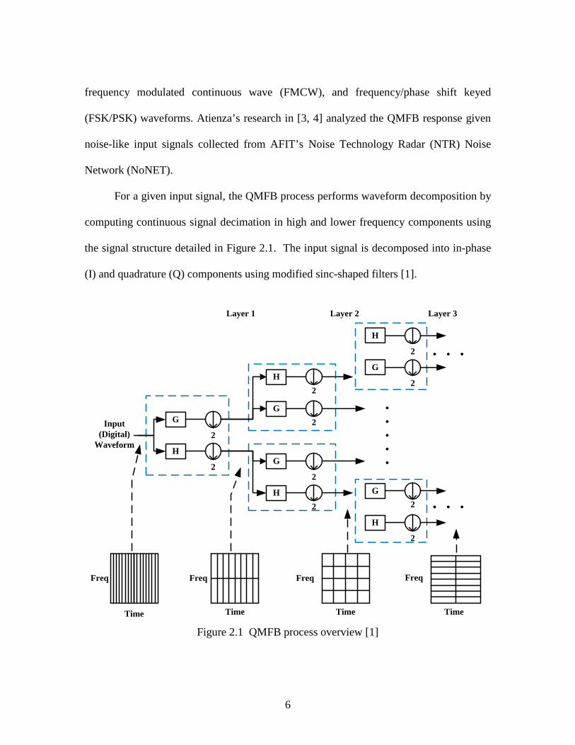
signal duration as well as time and frequency allocation. As detailed in Figure 2.1, the
process adopted here was introduced by Pace [1] and subsequently exploited in additional
related works of Jarpa and Atienza [3, 4]. Jarpa’s research in [3] was based on verifying
QMFB response given structured signal inputs, including a single tone, multiple tone,
6
frequency modulated continuous wave (FMCW), and frequency/phase shift keyed
(FSK/PSK) waveforms. Atienza’s research in [3, 4] analyzed the QMFB response given
noise-like input signals collected from AFIT’s Noise Technology Radar (NTR) Noise
Network (NoNET).
For a given input signal, the QMFB process performs waveform decomposition by
computing continuous signal decimation in high and lower frequency components using
the signal structure detailed in Figure 2.1. The input signal is decomposed into in-phase
(I) and quadrature (Q) components using modified sinc-shaped filters [1].
G
H
H
GH
G
G
H G
H
2
2
2
2
2
2
2
2
2
2
Layer 1 Layer 2 Layer 3
Input (Digital)
Waveform
Freq
Time TimeTimeTime
FreqFreqFreq
Figure 2.1 QMFB process overview [1]
7
The output of each filter “Layer” corresponds to the amplitude (real or complex)
or magnitude as a function Frequency-Time (F-T) parameters according to the input
signal. After each filtering stage, the signal is decimated so further layers can be
computed. Because of the decimation process, and the filter input signal being a function
of the previous layer, the initial time window (duration) is increased by a power of two
with every computation. On the other hand, the initial frequency window (bandwidth)
decreases according to the same power of two. This creates a tradeoff between the
different layers which could produce useful data for a given layer. Given the post-
filtering decimation, the total numbers of available layers (N) is a function of the initial
number of data samples (Ns) and given by:
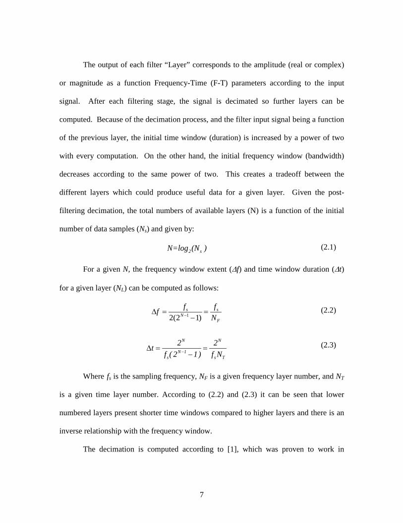
2 sN=log (N ) (2.1) For a given N, the frequency window extent (∆f) and time window duration (∆t)
for a given layer (NL) can be computed as follows:
12(2 1)s s
NF
f ffN−∆ = =
− (2.2)
N N
N 1s s T
2 2tf ( 2 1) f N−∆ = =
− (2.3)
Where fs is the sampling frequency, NF is a given frequency layer number, and NT
is a given time layer number. According to (2.2) and (2.3) it can be seen that lower
numbered layers present shorter time windows compared to higher layers and there is an
inverse relationship with the frequency window.
The decimation is computed according to [1], which was proven to work in

8
previous works [3, 4] and it consist in the implementation of a “modified sinc” finite
impulse response (FIR) given by:
S n+0.5 N (N-2)h[n]= sinc w[n], - n ,2 C 2 2
≤ ≤
(2.4)
Where S is the scaling variable, C is the compression variable, N is the number of
coefficients, and w[n] is a Hamming window weighting.
These particular filters have a flat bandpass response and pass the maximum
amount of desired signal energy at each layer. According to [1, 3] with an aim of getting
“nearly orthogonal filters with cross-correlation of less than 0.001” using N = 512, the
constant compression and scaling values in (2.4) are C=1.99375872338059 and
S=1.00618488680080. The Hamming window is use to suppress the effects of Gibb’s
phenomena resulting from sequence truncation [1, 3].
To avoid data sample loss, and because the total number of available layers is
given by (2.1), the following assumption has been made to compute, as initial
approximation, the total number of available layers for a given input signal:
2 sN=ceil[log (N )] (2.5)
Where N is the total number of available layer, Ns is the number of samples, and
the ceil[ ] operation ensures zero-padding to the next power of two.
2.3 Orthogonal Frequency Division Multiplexing (OFDM) signals
The sub-carrier frequencies in OFDM are chosen to be mutually orthogonal and
inter-carrier guard bands are not required as in basic modulation process. This simplifies
the transmitter and receiver designs; unlike conventional FDM, which requires a separate

9
filter for each sub-channel.
Considering the frequency domain, an OFDM symbol is made up multiple
subcarriers, the number of which determines the Fast Fourier Transform (FFT) size used.
As illustrated in Figure 2.2 [12] there are three distinct types of subcarriers used. The
type of subcarrier and purpose are as follows:
• Data Subcarriers: Data Transmission
• Pilot Subcarriers: Signal Estimation
• Null Carriers: No transmission; guard bands and DC subcarrier.
DC subcarrierData Subcarriers Pilot subcarriers
ChannelGuard Band Guard Band
Figure 2.2 OFDM frequency structure [12]
Considering time domain, an Inverse Fourier Transform (IFT) creates the OFDM
waveform where the signal time duration (Ts) is the result of the initial Guard Time (Tg)
plus the useful symbol time (Tb). A Tg copy of the last useful symbol is added and used
to correct for multipath. Therefore, the basic OFDM time structure is given by Figure
2.3.

10
Tg Tb
Ts
Figure 2.3 OFDM time structure [12]
The resultant transmitted signal is given by
s(t)= Re
⎝
⎛ej2πfct � ckej2πkΔf�t -Tg�
Nused2
k=-Nused2 , k≠0 ⎠
⎞ (2.6)
Where fc is the center carrier frequency, Nused is the number of used subcarriers, ck
is a complex modulation number specifying a point in the QAM signaling constellation,
Δf is the subcarrier spacing, t is the elapsed time since the beginning of the OFDM
symbol, and Tg = GxTb with defined G ∈ [1/4, 1/8, 1/16, 1/32] [12].
According to the OFDM frequency and time definitions given above, an OFDM-
based signal is generated as given by Figure 2.4
s(t)FFT -1
DAC
DAC
90°
X0
XN-1
XN-2
X1 fc
R
C
s[n]
Figure 2.4 OFDM-Based Signal Generation Process
11
2.3.1 OFDM-Based 802.11a Wi-Fi Signal
This OFDM-based signal is widely used in the implementation of wireless local
area networks (WLAN). According to [9] and related to this research effort, the OFDM
802.11a signal covers the following frequencies 5.15–5.25 GHz, 5.25–5.35 GHz, and
5.725–5.825 GHz. This provides a wireless LAN with data payload communication bit
rates of Rb ∈ [6, 9, 12, 18, 24, 36, 48, 54] Mbit/s. The system uses Ns = 52 subcarriers
that are modulated using binary phase shift keying (BPSK), quadrature phase shift keying
(QPSK) or 16-ary, 64-ary quadrature amplitude modulation (16-QAM or 64-QAM). The
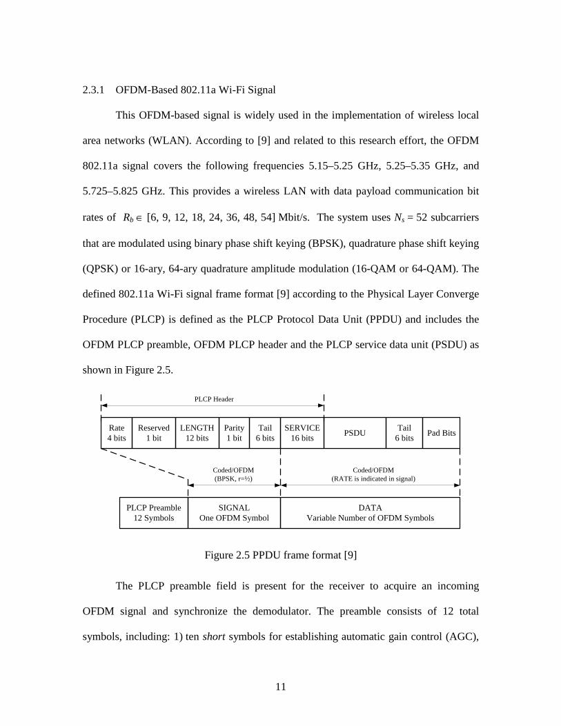
defined 802.11a Wi-Fi signal frame format [9] according to the Physical Layer Converge
Procedure (PLCP) is defined as the PLCP Protocol Data Unit (PPDU) and includes the
OFDM PLCP preamble, OFDM PLCP header and the PLCP service data unit (PSDU) as
shown in Figure 2.5.
PLCP Preamble 12 Symbols
DATAVariable Number of OFDM Symbols
SIGNALOne OFDM Symbol
Coded/OFDM(RATE is indicated in signal)
Coded/OFDM(BPSK, r=½)
SERVICE16 bits PSDU Tail
6 bits Pad BitsTail6 bits
Parity1 bit
LENGTH12 bits
Reserved1 bit
Rate4 bits
PLCP Header
Figure 2.5 PPDU frame format [9]
The PLCP preamble field is present for the receiver to acquire an incoming
OFDM signal and synchronize the demodulator. The preamble consists of 12 total
symbols, including: 1) ten short symbols for establishing automatic gain control (AGC),

12
coarse carrier frequency estimation, and 2) two long symbols for fine frequency
acquisition in the receiver. The PLCP preamble structure is shown in Figure 2.6.
t1 t10t9t8t7t6t5t4t3t2 GI*2 T1 T2 GI SIGNAL GI Data 2GI Data 1
10 x 0.8 = 8 µs 2 x 0.8 + 2 x 3.2 = 8 µs 0.8+3.2=4 µs 0.8+3.2=4 µs 0.8+3.2=4 µs
8 + 8 = 16 µs
Signal Detect, AGC, Diversity selection
Coarse Freq.Offset EstimationTiming Synchronize
Channel and Fine FrequencyOffset Estimation
RateLength
Service + Data
Figure 2.6 802.11a Wi-Fi Signal preamble structure [9]
2.3.2 OFDM-Based 802.16e WiMAX Signal
This protocol is aimed to extend wireless range of previous WLAN protocols and
provide broadband connectivity for data and telecommunications. According to [12] and
related to this research effort, the OFDM 802.16e signals cover the frequency bands
below 11GHz. In this case, each data frame is divided in two subframes, including:
1) the down link (DL) subframe aimed to transmitting data and control messages to
specific subscriber station (SS) and 2) the up link (UL) subframe that is used by the
subscriber to transmit to the Base Station (BS). Each subframe can be modulated using
BPSK, QPSK, 16-QAM or 64-QAM. The defined 802.16e WiMAX Signal frame can be
formatted using either time division duplexing (TDD) or frequency division duplexing
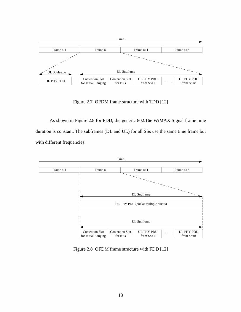
(FDD) techniques. As shown in Figure 2.7 for TDD, the generic 802.16e WiMAX Signal
frame time duration is obtained by adding each subframe (DL and UL) per SS.
13
Frame nFrame n-1 Frame n+2Frame n+1
DL PHY PDU UL PHY PDU from SS#1
Contention Slot for BRs
Contention Slot for Initial Ranging
UL PHY PDU from SS#k
Time
DL Subframe UL Subframe
Figure 2.7 OFDM frame structure with TDD [12]
As shown in Figure 2.8 for FDD, the generic 802.16e WiMAX Signal frame time
duration is constant. The subframes (DL and UL) for all SSs use the same time frame but
with different frequencies.
Frame nFrame n-1 Frame n+2Frame n+1
Time
DL PHY PDU (one or multiple bursts)
UL PHY PDU from SS#1
Contention Slot for BRs
Contention Slot for Initial Ranging
UL PHY PDU from SS#n
DL Subframe
UL Subframe
Figure 2.8 OFDM frame structure with FDD [12]

14
2.4 Summary
Technical background for the research effort has been presented, to include a
discussion of the QMBF process and characteristics. The total number of samples, sample
frequency and zero padding were described as key parameters aimed to achieve Δf and Δt
which allow reliable qualitative visual assessment according to the available generated
layers. Fundamentals of OFDM were introduced and two specific OFDM-based signals
of interest described. This included a discussion of relevant physical layer characteristics
for 802.11a Wi-Fi and 802.16e WiMAX signals.
15
CHAPTER 3.
Methodology
3.1 Introduction
This chapter discusses the adopted methodology aimed at performing the
necessary data and simulation management to satisfy defined objectives in this the
research effort. Section 3.2 provides the process overview which shows the main flow
diagram that was used as the baseline process for the research effort. Section 3.3
describes the verification and validation (V&V) signals used to ensure the QMFB process
was implemented correctly. This is followed by Section 3.4 which describes the OFDM-
based signals considered for demonstrating the exploitation capability of the QMFB
process. Implementation of the QMFB process is detailed in Section 3.5, to include the
effects of signal resampling and zero-padding for a given input signal. Finally, the
chapter concludes with Section 3.6, results presentation format, which shows how results
are presented for each case considered.
3.2 Process Overview
The flow diagram in Figure 3.1 was developed to set the sequence of steps aimed
at achieving the objectives described in Chapter 1 and based on background information
given in Chapter 2. The goal was to provide measurable results at every different stage
of the modeled problem. For each input, signal characteristics were first verified using
both time domain and frequency domain power spectral density (PSD) responses. Once
verified, the signal was input to the QMFB process and the resulting layer outputs were
used to exploit features. The exploitation assessment included two steps: 1) Seeing how

16
well resultant QMFB features match the 1-D time and PSD characteristics of the input
signal, and then 2) Using qualitative visual assessment to see if the 2-D QMFB F-T
outputs provided an additional insight on features not evident in 1-D responses.
QMFB
Resampling and/or Zero
padding
Signal Verification & Validation
Layer Plotting and Analysis
RequiredTime/Frequency
Resolution
NO
Qualitative Visual Assessment
Validation and Verification signals
802.16e signal
802.11a signal
QMFB PROCESS
COLLECTION POST-COLLECTION
RESULTSYES
Figure 3.1 Overview of Research Methodology 3.3 Verification and Validation (V&V) signals
To ensure the QMFB process was implemented correctly, QMFB output
responses were looked at using two specific input signals for V&V. The two analytic
V&V signals included a continuous LFM-modulated signal and a discrete multi-tone

17
signal used for V&V in previous work [1, 3, 4]. The signal’s characteristics presented on
each V&V signals are aimed to realize differences on the QMFB response due to
continuous modulation, discrete modulation, and single versus multiple frequencies.
Signal generation parameters for each of the V&V signal are set to establish identical
QMFB processing parameters as provided in Table 3.1
Table 3.1 QMFB Parameters for V&V Signal Processing
Bandwidth (KHz)
Samp Freq fs (Hz)
Duration (mSec)
Number of Samples
40 100 1.6 2428
3.3.1 Continuous Linear FM (LFM) signal
The LFM V&V signal was used to assess the QMFB response to a continuous
signal input having a linear frequency and amplitude change during the signal duration
[2]. The signal time and PSD response is shown in Figure 3.2 were generated using the
analytic expression in (3.1) with fL = 45 KHz , fH = 95KHz, and
f∆ = (FL − FH) = −50 KHz.
s1(t) = A1 sin�2πfHt� 0 < t < 0.6 m s2(t) = A2(t) sin�2πf∆t2� 0.6 m ≤ t < 1.0 m s3(t) = A3 sin�2πfLt� 1.0 m ≤ t < 1.6 m
sLFM(t) =� si(t)3
i=1
(3.1)

18
Figure 3.2 Analytic LFM V&V signal time domain and PSD responses.
3.3.2 Discrete Multi-Tone (DMT) V&V Signal
The DMT V&V signal was generated consistent with Szmajda’s V&V signal in
[7] and was chosen to assess the QMFB response to a discrete modulated signal having
both single and multiple frequency components across time. The signal time and PSD
responses are shown in Figure 3.3 and were generated using the analytic expressions in
(3.2) and tone parameters provided in Table 3.2
s1(t) = A1 sin�2πf1t� 0 < t < 13 s2(t) = A2 sin�2πf2t� 13 < t < 25
s3(t) = 0 25 < t < 37
s4(t) = s1(t) 37 < t < 50s5(t) = A5 sin�2πf5t� 37 < t < 50s6(t) = A6 sin�2πf6t� 37 < t < 50
sDMT(t)=� si(t)6
i=1
(3.2)

19
Table 3.2 Discrete Multi-Tone Szmajda Signal Generation Parameters
Tone s1(t) s2(t) s4(t) s5(t) s6(t)
Amplitude 230√2 2A1 A1 A1 A1
Frequency (Hz) 5 5 5 10 40
Figure 3.3 Analytic DMT Szmajda V&V signal time domain and frequency responses.
3.4 OFDM-Based Signals
The QMFB response to the V&V signals described in Section 3.2 and Section 3.3
provide a baseline for assessing QMFB exploitation potential using two OFDM-based
signals. Each signal was decomposed according to its specific characteristics in order to
find, evaluate and exploit different responses. The two signals considered include
experimentally collected 802.11a Wi-Fi [8] and 802.16e WiMAX [0, 11] signals.

20
3.4.1 802.11a Wi-Fi signal
This OFDM signal was chosen because of its well-known and structured physical
layer response as described in Chapter 2. In this case, the signal used corresponds to
experimental collections taken to support results in [8]. The signal was analyzed in three
stages using 1) an isolated preamble response, 2) a single burst response and 3) an
integrated burst response.
During the first analysis stage the 802.11a preamble response was isolated and
only the first 10 short symbols corresponding to the first half of the preamble was
considered. During the second analysis stage, the response of a single 802.11a burst was
set as input to the QMFB process. Finally, burst integration was computed considering
the mean amplitude response for NB = 500 burst collections. The 802.11a Wi-Fi signal
parameters for each analysis case are presented in Table 3.3
Table 3.3 802.11a Wi-Fi Signal Parameters
Input Bandwidth
(MHz) Samp Freq fs (MHz)
Duration (µSec)
Number of Samples
Preamble 8.0 23.75 135 3200
Burst 9.0 23.75 124 2945
3.4.2 802.16e WiMAX signal
This signal was chosen to assess the QMFB response using a more complex
structured OFDM-based signal input. In this case, the input signal corresponds to
experimental collections made in support of work in [0, 11]. The process is aimed to
exploit the physical layer parameters and structure described in Chapter 2 according to
[12]. The experimental 802.16e WiMAX signal was analyzed in two stages. First, the
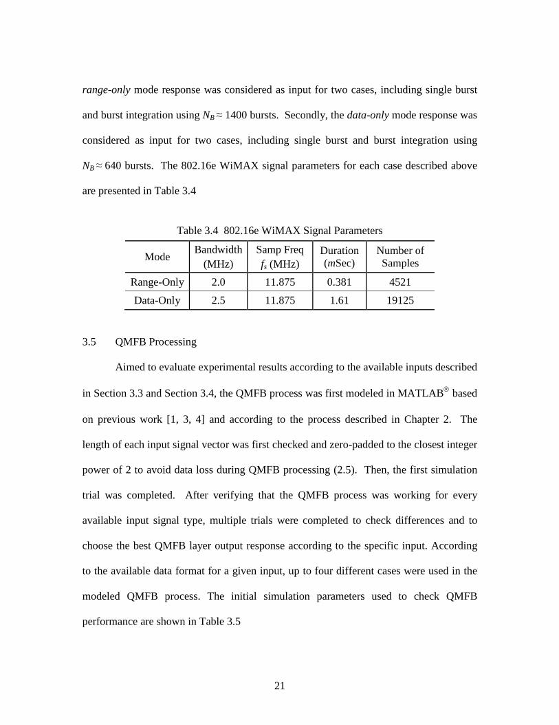
21
range-only mode response was considered as input for two cases, including single burst
and burst integration using NB ≈ 1400 bursts. Secondly, the data-only mode response was
considered as input for two cases, including single burst and burst integration using
NB ≈ 640 bursts. The 802.16e WiMAX signal parameters for each case described above
are presented in Table 3.4
Table 3.4 802.16e WiMAX Signal Parameters
Mode Bandwidth
(MHz) Samp Freq fs (MHz)
Duration (mSec)
Number of Samples
Range-Only 2.0 11.875 0.381 4521
Data-Only 2.5 11.875 1.61 19125
3.5 QMFB Processing
Aimed to evaluate experimental results according to the available inputs described
in Section 3.3 and Section 3.4, the QMFB process was first modeled in MATLAB based
on previous work [1, 3, 4] and according to the process described in Chapter 2. The
length of each input signal vector was first checked and zero-padded to the closest integer
power of 2 to avoid data loss during QMFB processing (2.5). Then, the first simulation
trial was completed. After verifying that the QMFB process was working for every
available input signal type, multiple trials were completed to check differences and to
choose the best QMFB layer output response according to the specific input. According
to the available data format for a given input, up to four different cases were used in the
modeled QMFB process. The initial simulation parameters used to check QMFB
performance are shown in Table 3.5

22
Table 3.5. Initial QMFB Configuration
Input Real (R), Complex(C), Magnitude # Filter Coefficients 512
Window Hamming fs Initial Sample Frequency
Total # QMFB Layers Ceil{log2[length(input)]} Given an input vector to the QMFB process, the first “Layer” output is computed,
decimated, stored, and passed to the next layer. This iterative process repeats and ends
after the initial vector is decimated according to:
NL=log2(Data Length)=Total # Available Layers (3.3)
Because data length is a function of both sampling frequency (fs) and total signal
duration (Ts), two pre-conditioning steps were included in the QMFB process, henceforth
referred to as resampling and zero-padding. Thus, each input signal was resampled, zero-
padded and set as input to the QMFB process to achieve the desired frequency and time
resolution in a given QMFB layer output. According to the QMFB frequency-time
tradeoff described in Chapter 2, better time resolution is achieved in lower QMFB layers,
but better frequency resolution is achieved in higher QMFB layers. So the challenge is to
find a frequency sampling rate (fs) versus signal duration (Ts) aimed to present an
accurate representation of input signal characteristics. Henceforth, this is called the “the
most representative layer” which corresponds to the layer which shows frequency and
signal time allocation that could be useful to exploit input signal features such as signal
bandwidth (W), signal duration (Ts), time resolution (Δt) and frequency resolution (Δf).
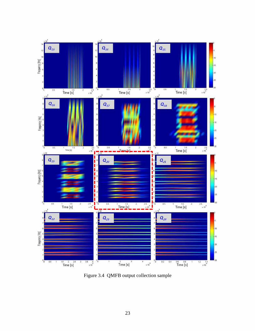
Figure 3.4 shows a collection of QMFB outputs where “the most representative layer”
corresponds to layer #20 (Q20) highlighted in the red dashed rectangle.
23
Figure 3.4 QMFB output collection sample
24
3.5.1 Signal Resampling
By resampling the input signal, the number of available input data samples
increases without changing the total signal duration Ts. This also increases the effective
sampling frequency fs and because of the F-T trade-off in QMFB processing, it is
expected that “the most representative layer” should be located in upper layers, which
increases required computing time and time resolution Δt for a given input signal.
3.5.2 Zero Padding
By zero-padding the input signal, the total effective time duration Ts is increased,
so better frequency resolution is achieved for a given signal and it is expected that the
most representative layer is now located in lower layers. But lower layers present poorer
signal frequency resolution (increased Δf), therefore by using lower layer analysis results
could be an inaccurate signal representation.
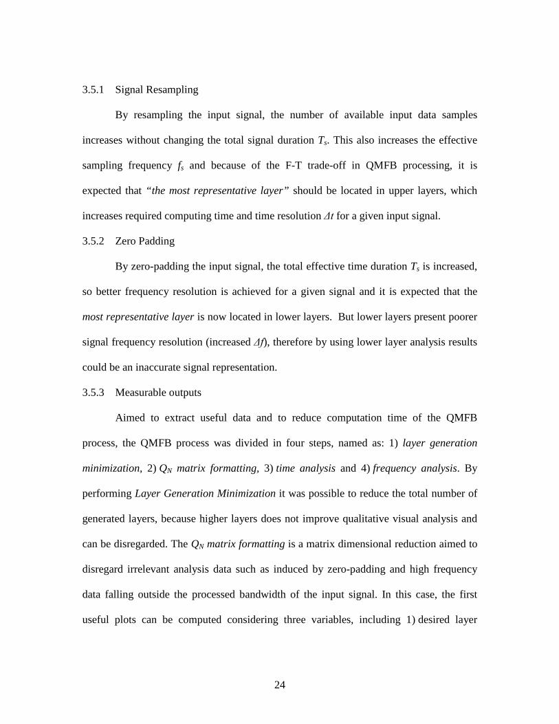
3.5.3 Measurable outputs
Aimed to extract useful data and to reduce computation time of the QMFB
process, the QMFB process was divided in four steps, named as: 1) layer generation
minimization, 2) QN matrix formatting, 3) time analysis and 4) frequency analysis. By
performing Layer Generation Minimization it was possible to reduce the total number of
generated layers, because higher layers does not improve qualitative visual analysis and
can be disregarded. The QN matrix formatting is a matrix dimensional reduction aimed to
disregard irrelevant analysis data such as induced by zero-padding and high frequency
data falling outside the processed bandwidth of the input signal. In this case, the first
useful plots can be computed considering three variables, including 1) desired layer
25
number, 2) upper frequency limit, and 3) upper time limit. The resultant output Q_n.mat
file was created (were n denotes a given layer number) considering an amplitude (real or
complex) matrix, a magnitude matrix, Δt and Δf values for a given layer, time vector,
frequency vector and fs. The time analysis and frequency analysis steps permit
comparison of input data and QMFB responses in order to realize process accuracy and
losses due to the signal processing. Figure 3.5 shows all the available measurable outputs
and their relation to the QMFB computing process.
Qualitative Visual Assessment
Input Signal Layer Generation
Layer Plotting
Q Matrix Generation
Amplitude Matrix
Magnitude Matrix
Time Analysis
Frequency Analysis
Time Response
Frequency Response
Overlaid Time
Response
Overlaid Frequency Response
Figure 3.5 Measurable process outputs
3.5.4 Presentation of QMFB Layer Outputs
Aimed to the objective of providing QMFB qualitative visual assessment, the
results are presented in frequency versus time (F-T) plots for “the most representative
layer” along with the average frequency and average time plot of the input processed

26
signal. The QMFB layer output data can be presented in many formats. For clarity and
to enable consistent comparison as the input signal varies, all results presented in
Chapter 4 use the format presented in Figure 3.6 which includes numbered responses of:
1. The normalized average frequency response computed as a row-wise average for
a given QMFB layer data.
2. “The most representative layer”, corresponds to a 2D QMFB F-T layer output
plotted using Matlab® pcolor function followed by shading interp. Appendix B
contains a complete set of 2D F-T for given signal.
3. The normalized average time response computed as a column-wise average for a
given QMFB layer data.
Figure 3.6. Representative Presentation Layout for a given QMFB layer output showing
(1) 1-D Average Frequency, (2) 2-D QMFB, and 1-D Average Time responses
Note: For Chapter 4 results, the plots correspond to three different QMFB layers identified as the most representative responses for a given domain.

27
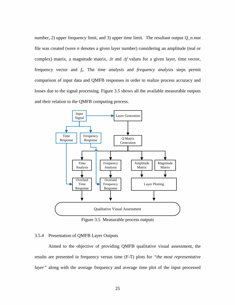
3.5.5 Single Burst vs. Integrated Bursts Overlay Plots
Aimed to check QMFB response related to a given signal input, average plots for
both time (Figure 3.7) and PSD (Figure 3.8) responses are provided to assess process
accuracy and signal processing loses. The following two plots are representative of the
presentation format used in Chapter 4.
Figure 3.7 Overlay Time responses showing input signal response, QMFB output
for single and integrated burst
28
Figure 3.8 Overlay Frequency responses showing input signal response, QMFB
output for single and integrated burst 3.6 Summary
The methodology presented in this chapter was applied to each of the described
input signals. To reduce computation time, the QMFB process was decomposed and
measurable outputs at each stage were defined. Using the designed process flow diagram
in Figure 3.5, different layers output data are generated, saved and analyzed using
qualitative visual assessment to characterize QMFB potential for exploiting unknown
signals. The effectiveness of this method is based on signal parameters such as the
resampling vector, zero-padding factor, total signal duration, time resolution Δt and
frequency resolution Δf for each computed QMFB layer.

29
CHAPTER 4.
Simulation Results and Analysis
4.1 Introduction
This chapter presents MATLAB simulation results and data analysis based on
that was obtained using the methodology discussed in Chapter 3. Baseline verification
and validation (V&V) performance of the QMFB process is first addressed in Section 4.2
using the LFM and analytic Szmajda signals described in Chapter 2. Then, OFDM based
signals described in Chapter 2 are input to the QMFB process to determine if visually
discernible features are present for estimating signal parameters. The QMFB results are
presented in frequency versus time (F-T) plots for a given layer previously defined in
chapter 3 as “the most representative layer”, along with individual average time and
frequency responses. Finally, overlaid plots are presented to compare QMFB process
outputs for single burst and integrated burst responses.
4.2 Process V&V Signals
Performance assessment is first performed with the LFM and analytic Szmajda
signals described in Chapter 2 input to the QMFB process. QMFB performance is
characterized trough qualitative visual assessment using joint 2D F-T responses as well
as independent 1D frequency and time responses.
4.2.1 LFM-Based V&V Signal
The normalized time and frequency responses for the input LFM-based signal are
presented in Figure 4.1. The signal was resampled and zero-padded prior to QMFB
processing according to the values shown in Table 4.1. The LFM signal time response

30
shows that higher frequencies are located in the first half of the signal, after those lower
frequency responses are present. Related to the PSD response, it can be seen that the
W−30dB bandwidth is located within the f = 40 KHz to f = 100 KHz range. Two
frequencies, f = 45 KHz and f = 95 KHz, are present with higher power levels of P = 0 dB
and P = -4 dB, respectively. For the rest of the frequencies between the two power peaks
it can be seen that there is an inverse relationship between the frequency and signal
power, with power decreasing from P = -16 dB to P = -19 dB.
Figure 4.1 LFM V&V signal time domain and PSD responses.
Table 4.1 LFM V&V Signal Parameters
Input Bandwidth
(Hz) Samp Freq
fs (Hz) Duration
(Sec) Number of Samples
Sample Rate
Zero Padding
Original 6.0 x 10⁴ 1.5 x 10⁸ 1.62 x 10⁻³ 2428 1 N/A Resampled 6.0 x 10⁴ 1.2 x 10¹¹ 3.50 x 10⁻³ 1942400 800 222

31
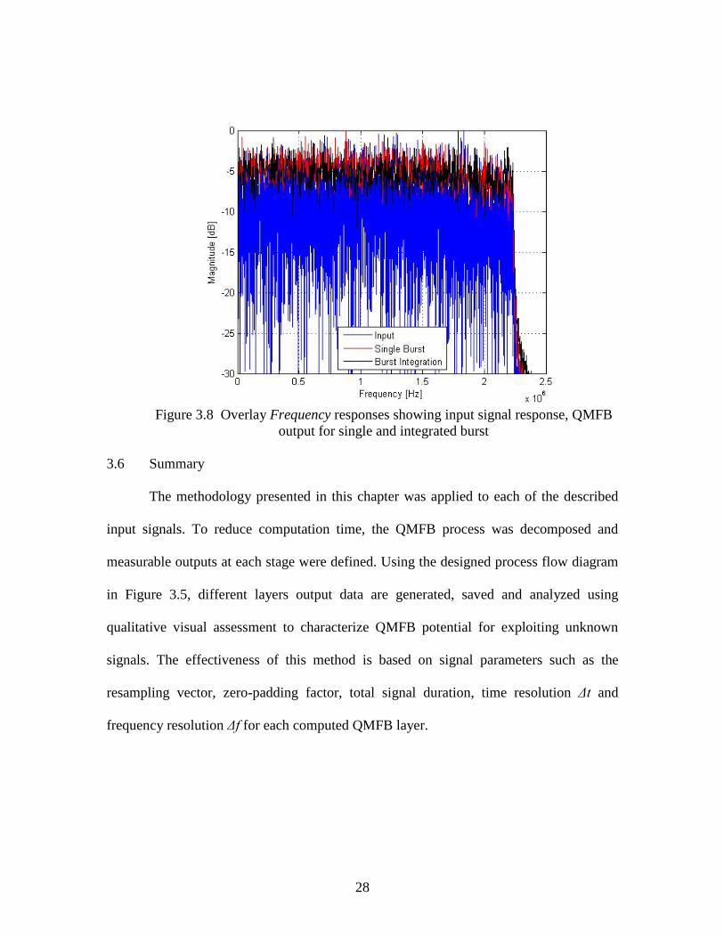
After pre-processing the LFM signal according to parameters in Table 4.1, the
signal was input to the QMFB process. Representative QMFB results for Layer #14 are
presented in Figure 4.2 with the signal’s linear frequency behavior highlighted (yellow
arrows) and power distributed according to color bar. The estimated frequency and time
resolution parameters were computed from the F-T plot in Figure 4.2 as Δf ≈ 36.62 KHz
and Δt ≈ 1.36x10⁻⁵ s. It can be seen that the signal frequency starts and remains at
f = 95 KHz until t = 0.65 ms, at which time the frequency decreases linearly to t = 1 ms.
At t = 1 ms the frequency is f = 45 KHz which remains constant until the end of the
signal. It also can be seen that the peak signal power is higher in the lower frequency of
f = 45 KHz and for f = 95 KHz the average power is approximately -3.0 dB compared to
the maximum signal power. By comparison with analytic signal responses shown in
Figure 4.1, the QMFB frequency and time averages show that the process, with some
degradation and signal processing loses due to the computing processing and the instant
changes of signal frequency, are consistent.
32
Figure 4.2. QMFB Layer #14 output for LFM V&V signal. Average PSD plot based on
Layer #14 as presented and average time plot based on Layer #10.
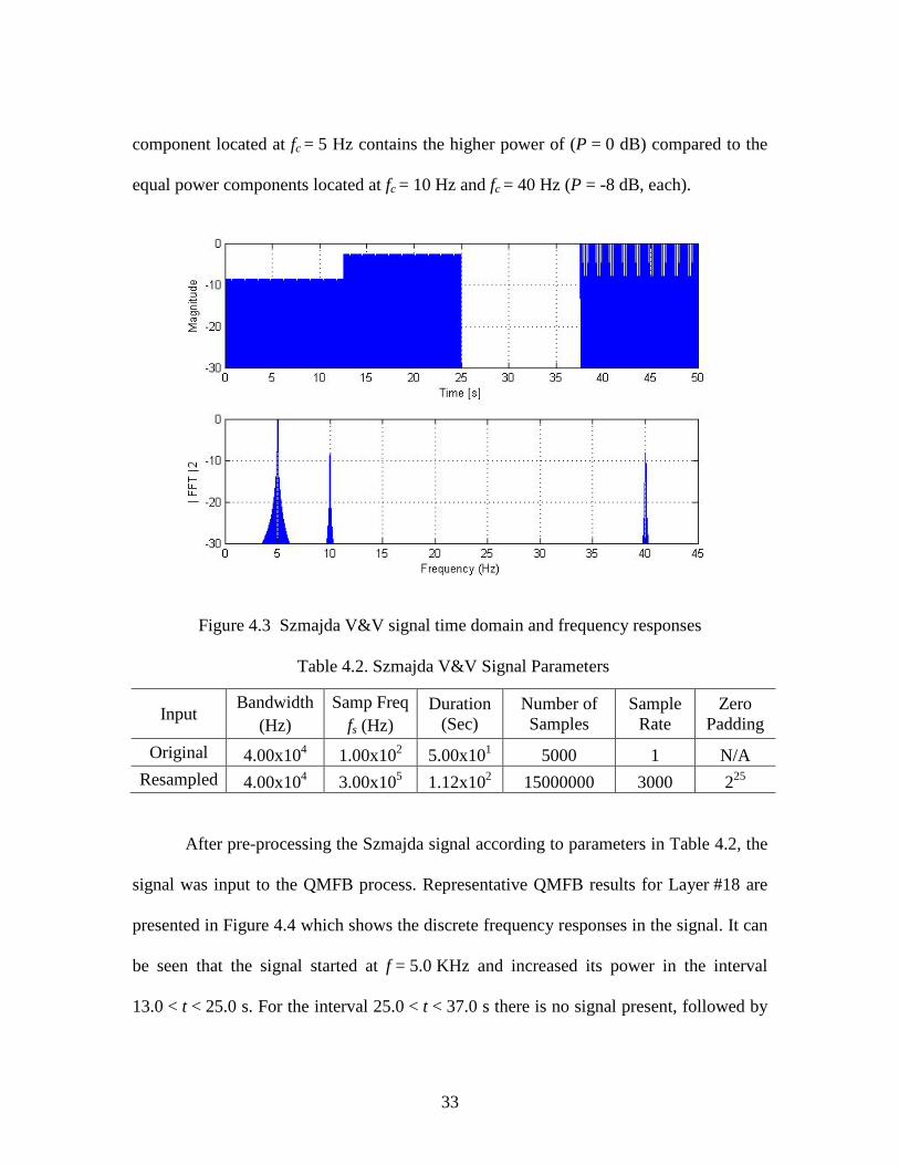
4.2.2 Analytic Szmajda V&V Signal
The normalized time and frequency responses for the analytic Szmajda signal are
presented in Figure 4.3. The signal was resampled and zero-padded prior to QMFB
processing according to the values shown in Table 4.2. Related to the time response, four
different signal magnitudes can be seen. Besides the absence of a signal response in the
t = 25 s to t = 37 s interval, no other noticeable parameters can be identified. Related to
the PSD response, it can be seen that considering the W−30dB bandwidth, three carrier
frequencies are present, including fc = 5 Hz, fc = 10 Hz and fc = 40 Hz. The signal
33
component located at fc = 5 Hz contains the higher power of (P = 0 dB) compared to the
equal power components located at fc = 10 Hz and fc = 40 Hz (P = -8 dB, each).
Figure 4.3 Szmajda V&V signal time domain and frequency responses
Table 4.2. Szmajda V&V Signal Parameters
Input Bandwidth
(Hz) Samp Freq
fs (Hz) Duration
(Sec) Number of Samples
Sample Rate
Zero Padding
Original 4.00x10⁴ 1.00x10² 5.00x101 5000 1 N/A Resampled 4.00x10⁴ 3.00x10⁵ 1.12x10² 15000000 3000 225
After pre-processing the Szmajda signal according to parameters in Table 4.2, the
signal was input to the QMFB process. Representative QMFB results for Layer #18 are
presented in Figure 4.4 which shows the discrete frequency responses in the signal. It can
be seen that the signal started at f = 5.0 KHz and increased its power in the interval
13.0 < t < 25.0 s. For the interval 25.0 < t < 37.0 s there is no signal present, followed by

34
the interval 37.0 < t < 50.0 s from 37 s to 50 s when three frequencies are present
(f = 5.0 KHz, f = 10.0 KHz, and f = 40.0 KHz). The estimated frequency and time
resolution parameters were computed from the F-T plot in Figure 4.4 as Δf ≈ 0.57 KHz
and Δt ≈ 0.88 s. For the average frequency and time plots, the parameters are
Δf ≈ 0.57 KHz and Δt ≈ 13.65 ms, respectively. By comparing analytic signal responses
in Figure 4.3, both the average frequency and time responses from the QMFB process,
with some degradation and loses due to the computing processing, was consistent.
Figure 4.4. QMFB Layer #18 output for Szmajda V&V signal. Average PSD plot based on Layer #18 as presented and average time plot based on Layer #12.

35
After processing and analyzing QMFB performance using the V&V signals, it
was concluded that the QMFB process is able to effectively process different types of
signals and produce outputs matching theoretical expected results. However, some pre-
QMFB filtering artifacts appeared due to the effects of instantaneous frequency on filter
performance. Beside the artifacts, the QMFB results presented an acceptable response in
frequency and time allocation within the middle layers.
4.3 OFDM-Based Signal Performance
The two OFDM-based signals described in Chapter 2 were used as input to the
QMFB process and simulation performed according to the methodology explained in
Chapter 3. Results for 802.11a Wi-Fi and 802.16e WiMAX OFDM-based signals are
presented and QMFB output reliability assessed relative to input signal features. Overlay
plots are computed to compare input signal and QMFB output responses for single burst
and integrated burst response cases.
4.3.1 Experimental 802.11a Wi-Fi Signal
Experimental 802.11a Wi-Fi signal assessment was performed using data
collected in support of previous work detailed in [8]. Collections were made using
AFIT’s RFSICS with the Wi-Fi devices operating in an anechoic chamber environment.
According to the structure of this signal described in Chapter 2, the 802.11a signal is
composed of two distinct regions. The preamble region is used for network
synchronization, timing, control, etc., and the payload region is used for transferring user
data. Per IEEE standards for 802.11a implementation [9], the preamble is further divided
into two distinct regions, with the first half containing 10 short OFDM symbols and the

36
second half containing 2 long OFDM symbols. The 10 short OFDM symbols region is
selected here for demonstration with a single burst sent to the QMFB process first and
then an integrated collection of bursts sent to the QMFB process.
4.3.1.1 802.11a Wi-Fi Preamble
The normalized time and PSD responses for 802.11a Wi-Fi preamble are shown
in Figure 4.5. The first ten symbols of the preamble were isolated, resampled and zero-
padded prior to QMFB processing according to the values shown in Table 4.3. Related to
the time response, the signal duration is approximate T = 8 µs and it can be seen that 10
peaks are very noticeable. Considering the W−30dB bandwidth, the PSD response shows
twelve distinct frequency components that match the 802.11a signal structure described
in Chapter 2.
Figure 4.5 Time and PSD responses for 10 short symbols 802.11a Wi-Fi preamble.
37
Table 4.3. 802.11a 10 short symbols set as input to QMFB
Input Bandwidth
(Hz) Samp Freq
fs (Hz) Duration
(Sec) Number of Samples
Sample Rate
Zero Padding
Original 8.00x10⁶ 2.38x10⁷ 1.35x10⁻⁴ 3200 1 N/A Resampled 8.00x10⁶ 2.38x10¹¹ 1.41x10⁻⁴ 32000000 10000 225
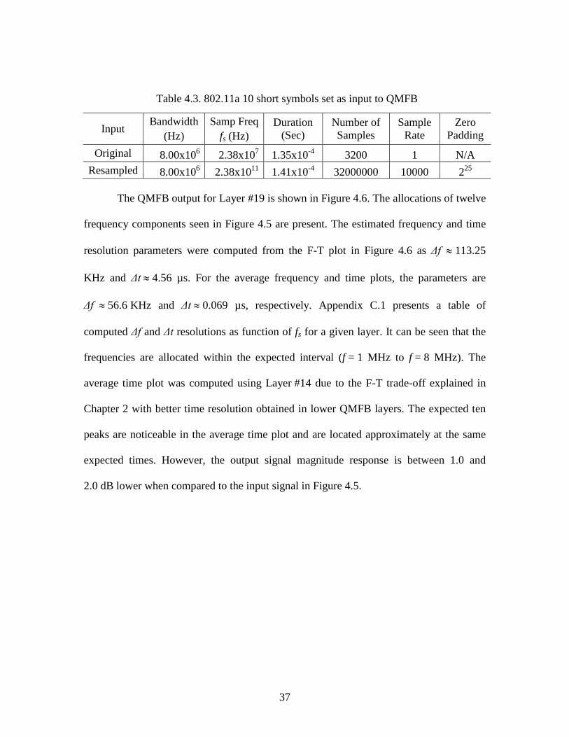
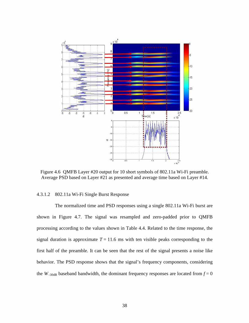
The QMFB output for Layer #19 is shown in Figure 4.6. The allocations of twelve
frequency components seen in Figure 4.5 are present. The estimated frequency and time
resolution parameters were computed from the F-T plot in Figure 4.6 as Δf ≈ 113.25
KHz and Δt ≈ 4.56 µs. For the average frequency and time plots, the parameters are
Δf ≈ 56.6 KHz and Δt ≈ 0.069 µs, respectively. Appendix C.1 presents a table of
computed Δf and Δt resolutions as function of fs for a given layer. It can be seen that the
frequencies are allocated within the expected interval (f = 1 MHz to f = 8 MHz). The
average time plot was computed using Layer #14 due to the F-T trade-off explained in
Chapter 2 with better time resolution obtained in lower QMFB layers. The expected ten
peaks are noticeable in the average time plot and are located approximately at the same
expected times. However, the output signal magnitude response is between 1.0 and
2.0 dB lower when compared to the input signal in Figure 4.5.
38
Figure 4.6 QMFB Layer #20 output for 10 short symbols of 802.11a Wi-Fi preamble. Average PSD based on Layer #21 as presented and average time based on Layer #14.
4.3.1.2 802.11a Wi-Fi Single Burst Response
The normalized time and PSD responses using a single 802.11a Wi-Fi burst are
shown in Figure 4.7. The signal was resampled and zero-padded prior to QMFB
processing according to the values shown in Table 4.4. Related to the time response, the
signal duration is approximate T = 11.6 ms with ten visible peaks corresponding to the
first half of the preamble. It can be seen that the rest of the signal presents a noise like
behavior. The PSD response shows that the signal’s frequency components, considering
the W−30dB baseband bandwidth, the dominant frequency responses are located from f = 0
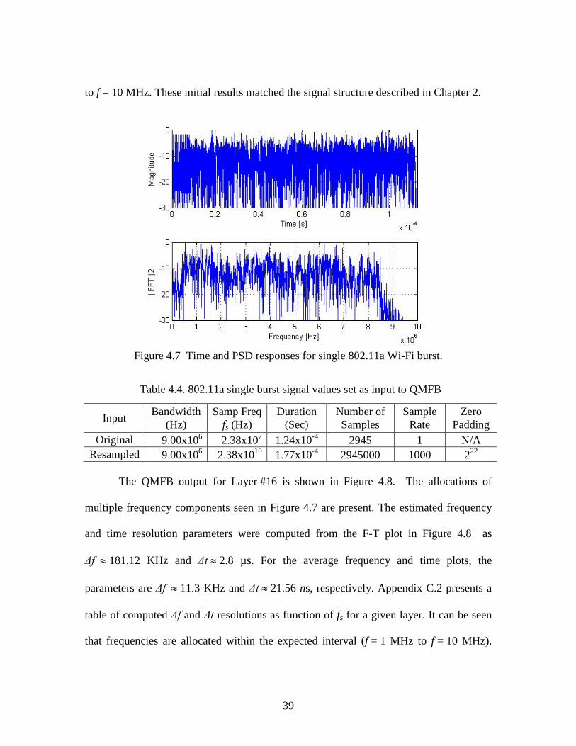
39
to f = 10 MHz. These initial results matched the signal structure described in Chapter 2.
Figure 4.7 Time and PSD responses for single 802.11a Wi-Fi burst.
Table 4.4. 802.11a single burst signal values set as input to QMFB
Input Bandwidth (Hz)
Samp Freq fs (Hz)
Duration (Sec)
Number of Samples
Sample Rate
Zero Padding
Original 9.00x10⁶ 2.38x10⁷ 1.24x10⁻⁴ 2945 1 N/A Resampled 9.00x10⁶ 2.38x10¹⁰ 1.77x10⁻⁴ 2945000 1000 222
The QMFB output for Layer #16 is shown in Figure 4.8. The allocations of
multiple frequency components seen in Figure 4.7 are present. The estimated frequency
and time resolution parameters were computed from the F-T plot in Figure 4.8 as
Δf ≈ 181.12 KHz and Δt ≈ 2.8 µs. For the average frequency and time plots, the
parameters are Δf ≈ 11.3 KHz and Δt ≈ 21.56 ns, respectively. Appendix C.2 presents a
table of computed Δf and Δt resolutions as function of fs for a given layer. It can be seen
that frequencies are allocated within the expected interval (f = 1 MHz to f = 10 MHz).

40
The first half of the preamble response is still noticeable and is located approximately at
the same expected times compared to the input shown in Figure 4.7.
According to the 802.11a signal parameters described in Chapter 2, there are
some signal features that can be extracted through qualitative visual assessment of the
QMFB output shown in Figure 4.8:
• The 10 short symbols shown in the left-hand red dashed rectangle
• The guard Interval shown in the right-hand red dashed rectangle
Figure 4.8 QMFB Layer #16 output for single 802.11a Wi-Fi burst. Average PSD based
on Layer #20 as presented and average time based on Layer #9.
41
4.3.1.3 Wi-Fi Integrated Burst Response
The normalized time and PSD responses for integrated 802.11a bursts are
shown in Figure 4.9. In this case, a total of NB = 500 802.11a burst responses were
integrated to create a new input to the QMFB process. The signal was resampled and
zero-padded prior to QMFB processing according to the values shown in Table 4.5.
Related to the time response, the signal duration is approximate T = 11.6 ms with ten
visible peaks corresponding to the first half of the preamble and the rest of the signal
presents a noise like behavior. The PSD response shows that the signal’s frequency
components, considering the W−30dB baseband bandwidth, the dominant frequency
responses are located from f = 0 to f = 10 MHz. These results match the signal structure
described in Chapter 2. It also can be seen that the first ten symbols show a uniform
magnitude, with the peak located at approximately at t = 2.4 µs corresponding to the
guard interval described in Chapter 2. The part of the signal corresponding to the payload
(user data) shows a magnitude reduction due to randomness of the symbol assignment.

42
Figure 4.9 Time and PSD responses for NB = 500 integrated bursts 802.11a Wi-Fi.
Table 4.5. 802.11a signal values for NB = 500 integrated bursts as input to QMFB
Input Bandwidth
(Hz) Samp Freq
fs (Hz) Duration
(Sec) Number of Samples
Sample Rate
Zero Padding
Original 9.00x10⁶ 2.38x10⁷ 1.24x10⁻⁴ 2945 1 N/A Resampled 9.00x10⁶ 2.38x10¹⁰ 1.77x10⁻⁴ 2945000 1000 222
The QMFB output for Layer #16 is shown in Figure 4.10for integration of
NB = 500 bursts. The allocation of multiple frequencies components seen in Figure 4.9 is
present. The estimated frequency and time resolution parameters were computed from the
F-T plot in Figure 4.10 as Δf ≈ 181.12 KHz and Δt ≈ 2.8 µs. For the average frequency
and time plots, the parameters are Δf ≈ 22.6 KHz and Δt ≈ 0.173 µs, respectively.
Appendix C.2 presents a table of computed Δf and Δt resolutions as function of fs for a
given layer. The first half of the preamble response is still noticeable and is located
approximately at the same expected times compared to the input shown in Figure 4.9.

43
According to the 802.11a signal parameters described in Chapter 2, there are
some signal features that can be extracted through qualitative visual assessment of the
QMFB output shown in Figure 4.10:
• The 10 short symbols shown in the left-hand red dashed rectangle
• Lower correlation in the payload (user data) region in the right-hand red
dashed rectangle
• Average signal power below -5.0 dB for the payload (user data) region
highlighted by a red arrow in the average time plot.
Figure 4.10 QMFB Layer #16 output for NB = 500 integrated Wi-Fi bursts. Average PSD plot based on Layer #19 as presented and average time plot based on Layer #12.

44
4.3.1.4 802.11a Wi-Fi Preamble: Single vs. Integrated Response
To assess the QMFB response relative to signal input features, average time and
frequency plots are provided in Figure 4.11 to Figure 4.14 for single burst and integrated
burst QMFP processing. Related to the overlaid time responses in Figure 4.11 and Figure
4.12, it can be seen that the QMFB output envelope matches the input time response for
both single and integrated burst cases. Therefore, the F-T plots computed during the
process are reliable for revealing 802.11a Wi-Fi signal characteristics. In the payload
(user data) region of the average time response (t > 200 µs), the power reduction for burst
integration is evident given the random signal structure in this region. Related to the
average PSD response presented in Figure 4.13 and Figure 4.14, the burst integration
resulted in gain of approximate G ≈ 3.0 dB when compared to the input signal or single
burst QMFB responses.
Figure 4.11 Average time responses for 802.11a Wi-Fi signal.

45
Figure 4.12 Average time responses for 802.11a Wi-Fi signal expanded region for
0 < t < 200 µs.
Figure 4.13 Average PSD responses for 802.11a Wi-Fi signal.

46
Figure 4.14 Average PSD responses for 802.11a Wi-Fi signal expanded region for
0 < f < 3 MHz.
4.3.2 Experimental 802.16e WiMAX Signal
Experimental 802.16e WiMAX signal assessment was performed using data
collected in support of previous work detailed in [0, 11]. The collections were obtained
using AFIT’s RFSICS with Alvarion BreezeMAX 5000 Mobile Subscriber (MS) devices
operating in a typical office environment [13]. According to the structure of this signal
described in Chapter 2, and experimental observations noted in [0, 11], the analysis was
divided in two parts. The first part only considers WiMAX range-only burst responses
and the second part considers only WiMAX data-only burst responses. For each of these
cases, QMFB processing is conducted using single burst and integrated burst responses.
47
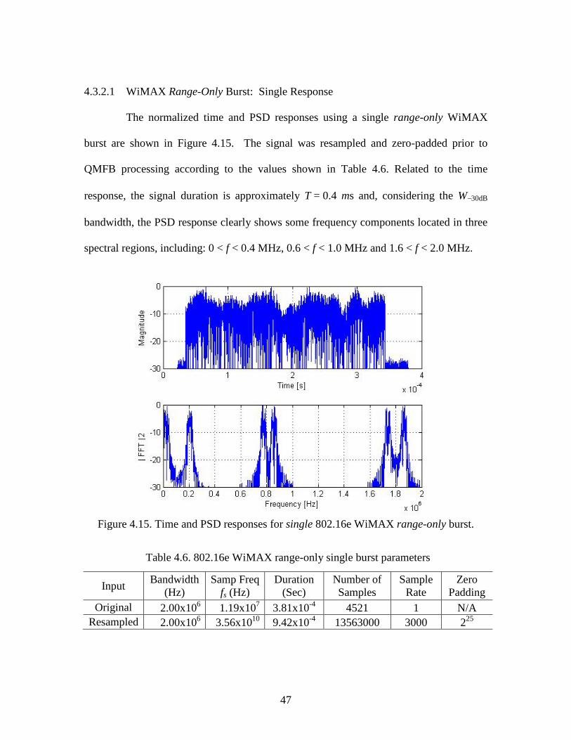
4.3.2.1 WiMAX Range-Only Burst: Single Response
The normalized time and PSD responses using a single range-only WiMAX
burst are shown in Figure 4.15. The signal was resampled and zero-padded prior to
QMFB processing according to the values shown in Table 4.6. Related to the time
response, the signal duration is approximately T = 0.4 ms and, considering the W−30dB
bandwidth, the PSD response clearly shows some frequency components located in three
spectral regions, including: 0 < f < 0.4 MHz, 0.6 < f < 1.0 MHz and 1.6 < f < 2.0 MHz.
Figure 4.15. Time and PSD responses for single 802.16e WiMAX range-only burst.
Table 4.6. 802.16e WiMAX range-only single burst parameters
Input Bandwidth (Hz)
Samp Freq fs (Hz)
Duration (Sec)
Number of Samples
Sample Rate
Zero Padding
Original 2.00x10⁶ 1.19x10⁷ 3.81x10⁻⁴ 4521 1 N/A Resampled 2.00x10⁶ 3.56x10¹⁰ 9.42x10⁻⁴ 13563000 3000 225

48
The QMFB output for Layer #18 is shown in Figure 4.16 for single 802.16e
WiMAX range-only burst. The allocation of six frequencies components seen in Figure
4.15 is present. The estimated frequency and time resolution parameters were computed
from the F-T plot in Figure 4.16 as Δf ≈ 67.9 KHz and Δt ≈ 7.4 µs. For the average
frequency and time plots, the parameters are Δf ≈ 16.9 KHz and Δt ≈ 0.115 µs,
respectively. Appendix C.3 presents a table of computed Δf and Δt resolutions as function
of fs for a given layer. It can be seen that frequencies are allocated within the three
expected intervals (0 < f < 0.4, 0.6 < f < 1.0, and 1.6 < f < 2.0 MHz), are distributed in
three pairs, and span the bandwidth shown in Figure 4.15. Within each pair of
frequencies a transition is seen between a certain numbers of transmitted symbols.

49
Figure 4.16 QMFB Layer #18 output for single 802.16e WiMAX range-only burst. Average PSD plot based on Layer #20 and average time plot based on Layer #12.
4.3.2.2 WiMAX Range-Only Burst: Integrated Response
The normalized time and PSD responses using integrated range-only WiMAX
bursts are shown in Figure 4.17. In this case, a total of NB = 1400 802.16e burst
responses were integrated to create a new input to the QMFB process. The range-only
integrated burst signal was resampled and zero-padded prior to QMFB processing
according to the same values previously shown in Table 4.6. Related to the time
response, the signal duration is approximately T = 0.4 ms and, considering the W−30dB

50
bandwidth, the PSD response contains the same frequency components as the single burst
response (0 < f < 0.4 MHz, 0.6 < f < 1.0 MHz and 1.6 < f < 2.0 MHz) plus some
additional frequency components below the P = -20 dB level.
Figure 4.17. Time and PSD responses for NB = 1400 integrated 802.16e WiMAX range-
only bursts. The QMFB output for Layer #18 is shown in Figure 4.18 for NB = 1400
integrated 802.16e WiMAX range-only bursts. The allocation of six frequencies
components seen in Figure 4.17 is present. The estimated frequency and time resolution
parameters were computed from the F-T plot in Figure 4.18 as Δf ≈ 67.9 KHz and
Δt ≈ 7.4 µs. For the average frequency and time plots, the parameters are Δf ≈ 16.9 KHz
and Δt ≈ 0.115 µs, respectively. Appendix C.3 presents a table of computed Δf and Δt
resolutions as function of fs for a given layer. It can be seen that frequencies are allocated
within the three expected intervals (0 < f < 0.4, 0.6 < f < 1.0, and 1.6 < f < 2.0 MHz), are

51
distributed in three pairs, and span the bandwidth shown in Figure 4.17. In this case, the
middle pair of frequencies presented the higher power correlation compared to the other
frequency components.
Figure 4.18 QMFB Layer #18 output for NB = 1400 integrated 802.16e WiMAX range-only bursts. Average PSD based on Layer #20 and average time based on Layer #12.
4.3.2.3 WiMAX Range-Only Burst: Single vs. Integrated Response
To assess the QMFB response relative to input signal features, average time and
frequency plots are provided in Figure 4.19 to Figure 4.22 for single burst and integrated
burst QMFP processing. Related to the overlay time response in Figure 4.19 and Figure
4.20, the integrated burst QMFB output show less energy in the time response due to

52
integration of random symbol assignment within and across every integrated burst.
Related to overlay PSD responses in Figure 4.21 and Figure 4.22, it can be seen that the
W−30dB bandwidth remains constant and that burst integration resulted in “thinner”
responses for the six frequency components.
Figure 4.19 Average time responses for 802.16e WiMAX range-only burst.

53
Figure 4.20 Average time responses for 802.16e WiMAX range-only burst. Expanded
region for 0 < t < 200 µs.
Figure 4.21 Average PSD responses for 802.16e WiMAX range-only burst.

54
Figure 4.22 Average PSD responses for 802.16e WiMAX range-only burst. Expanded region for 0 < f < 0.5 MHz.
4.3.2.4 802.16e WiMAX Data-Only Burst: Single Response
The normalized time and PSD responses using a single data-only 802.16e
WiMAX burst is shown in Figure 4.23. The signal was resampled and zero-padded prior
to QMFB processing according to the values shown in Table 4.7. Related to the time
response, the signal duration is approximate T = 1.6 ms and the noise like behavior of the
signal is seen in both time and frequency responses.

55
Figure 4.23 Time and PSD responses for single 802.16e WiMAX data-only burst.
Table 4.7. 802. 16e WiMAX data-only single burst parameters
Input Bandwidth (Hz)
Samp Freq fs (Hz)
Duration (Sec)
Number of Samples
Sample Rate
Zero Padding
Original 2.50x10⁶ 1.19x10⁷ 1.61x10⁻³ 19125 1 N/A Resampled 2.50x10⁶ 1.19x10¹⁰ 2.83x10⁻³ 19125000 1000 225
The QMFB output for Layer #16 is shown in Figure 4.24 for a single 802.16e
WiMAX range-only burst. The multiple frequency allocations shown in Figure 4.23 are
present. The estimated frequency and time resolution parameters were computed from
the F-T plot in Figure 4.24 as Δf ≈ 90.6 KHz and Δt ≈ 5.53 µs. For the average
frequency and time plots, the parameters are Δf ≈ 5.66 KHz and Δt ≈ 0.345 µs,
respectively. Appendix C.3 presents a table of computed Δf and Δt resolutions as function

56
of fs for a given layer. Other than bandwidth (W-30dB ≈ 2.25 MHz) and signal duration
(T ≈ 1.6 ms), no signal structure can be extracted from the F-T plot.
Figure 4.24 QMFB Layer #16 output for single 802.16e WiMAX data-only burst.
Average PSD based on Layer #20 and average time based on Layer #12. 4.3.2.5 802.16e WiMAX Data-Only Burst: Integrated Response
The normalized time and PSD responses for integrated data-only WiMAX
bursts are shown in Figure 4.25. The signal was resampled and zero-padded prior to
QMFB processing according to the values previously shown in Table 4.7. Related to the
time response, the signal duration is approximate 1.6 ms and it can be seen the noise like
behavior of the signal in both time and frequency responses.

57
Figure 4.25 Time and PSD responses for NB = 640 integrated 802.16e WiMAX data-
only bursts.
The QMFB output for Layer #16 is shown in Figure 4.26 for NB = 640 integrated
802.16e WiMAX data-only bursts. The allocation of multiple frequencies components
seen in Figure 4.25 is present. The estimated frequency and time resolution parameters
were computed from the F-T plot in Figure 4.26 as Δf ≈ 90.6 KHz and Δt ≈ 5.53 µs. For
the average frequency and time plots, the parameters are Δf ≈ 5.66 KHz and Δt ≈ 0.345
µs, respectively. Appendix C.3 presents a table of computed Δf and Δt resolutions as
function of fs for a given layer. Other than bandwidth (W-30dB ≈ 2.25 MHz) and signal
duration (T ≈ 1.6 ms), no signal structure can be extracted from the F-T plot.
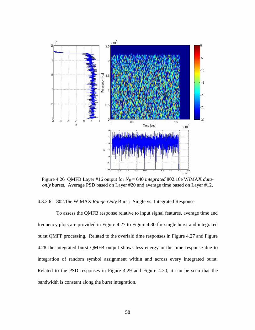
58
Figure 4.26 QMFB Layer #16 output for NB = 640 integrated 802.16e WiMAX data-only bursts. Average PSD based on Layer #20 and average time based on Layer #12.
4.3.2.6 802.16e WiMAX Range-Only Burst: Single vs. Integrated Response
To assess the QMFB response relative to input signal features, average time and
frequency plots are provided in Figure 4.27 to Figure 4.30 for single burst and integrated
burst QMFP processing. Related to the overlaid time responses in Figure 4.27 and Figure
4.28 the integrated burst QMFB output shows less energy in the time response due to
integration of random symbol assignment within and across every integrated burst.
Related to the PSD responses in Figure 4.29 and Figure 4.30, it can be seen that the
bandwidth is constant along the burst integration.
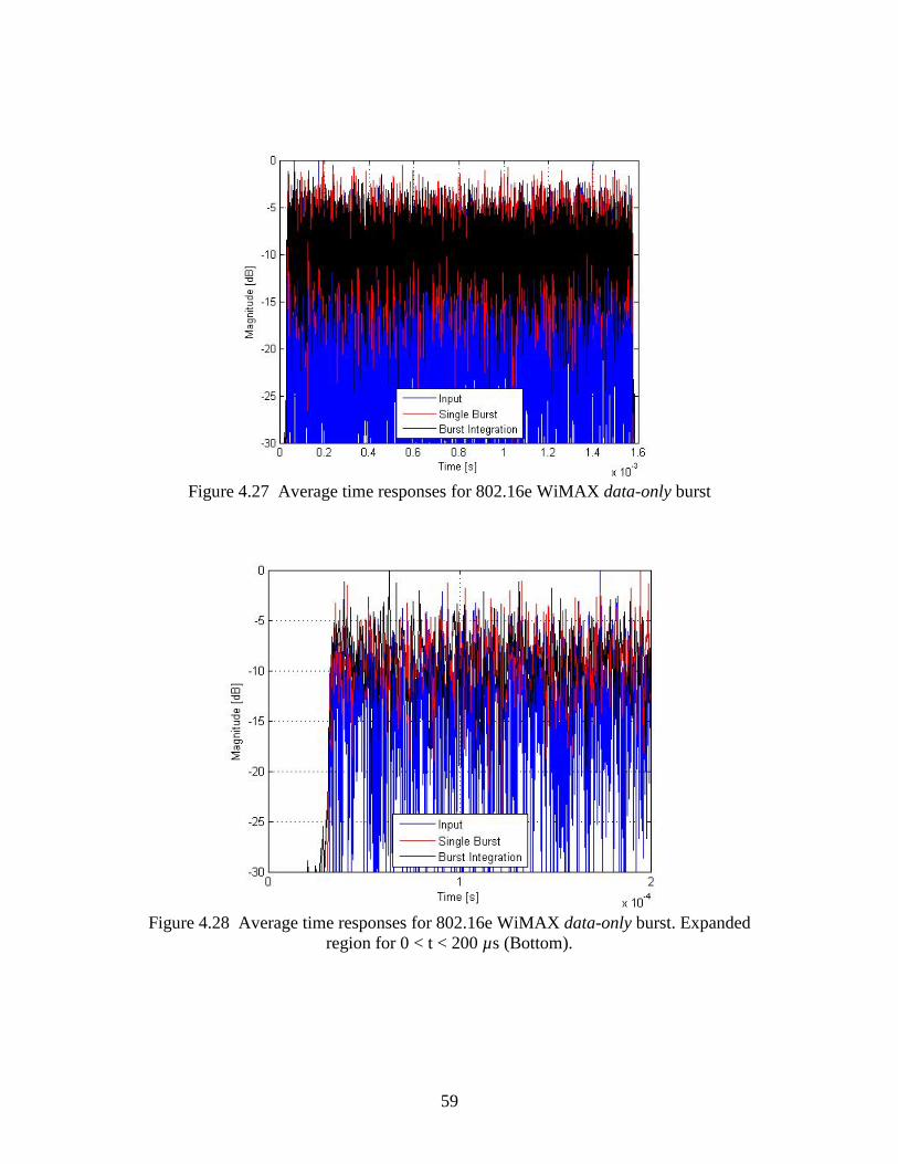
59
Figure 4.27 Average time responses for 802.16e WiMAX data-only burst
Figure 4.28 Average time responses for 802.16e WiMAX data-only burst. Expanded
region for 0 < t < 200 µs (Bottom).

60
Figure 4.29 Average PSD responses for 802.16e WiMAX data-only burst.
Figure 4.30 Average PSD responses for 802.16e WiMAX data-only burst. Expanded
region for 0 < f < 1.0 MHz.

61
4.4 Summary
The results presented in this chapter enabled qualitative visual assessment of
QMFB performance using each signal of interest. Related to the LFM and Szmajda V&V
signals, it was seen that the QMFB output offers reliable estimation of frequency and
time characteristics. Once the baseline was defined, verified and validated, experimental
OFDM-based signals were introduced and QMFB performance assessed. MATLAB
simulation results and qualitative visual analysis were sufficient for identifying some
signal features such as signal duration (TS) and bandwidth (W−30dB) while highlighting
relative signal structure.
Related to the analyzed 802.11a Wi-Fi signal, the preamble structure revealed by
QMFB processing is consistent with the theoretical description in Chapter 2. Using burst
integration, the effect of random symbol assignment during the payload (user data) region
became evident as lower magnitude responses in Figure 4.10. The average time and
average frequency plot showed that the QMFB output envelope followed the original
signal behavior, but average loses of approximate 1.0 dB for burst integration and 2.0 dB
for single burst were observed.
Related to the analyzed 802.16e WiMAX signal, the results are consistent with
the framework defined in Chapter 2 and the QMFB output for both the ranging-on and
data-only cases enabled qualitative visual assessment and provided some exploitation
benefit. Some key signal features such as bandwidth, frequency and time allocation were
extractable, and after further layer analysis approximations to symbol duration and
channel bandwidth were available.

62
CHAPTER 5.
Summary, Conclusions and Recommendations
This chapter presents a summary and conclusions of research findings along with
some recommendations for future work that have been extracted as result of this research
effort. The chapter is divided in three subsections: 1) Section 5.1 presents a summary
review related to the topics of interest covered during the research with some key
exploitation concepts highlighted relative to the overall process; 2) Section 5.2 presents
conclusions extracted from results after applying the adopted methodology in Chapter 3
and the baseline definitions given in chapter 2; and, 3) Section 5.3 is aimed at identifying
other applications for QMFB exploitation providing recommendations for future work.
5.1 Summary
Chapter 1 presented the operational and technical motivation along with the
research objectives. Related to the operational motivation, the approach was to provide a
qualitative visual assessment process for a given signal from an operator’s perspective.
By performing QMFB processing with a given signal it is possible to obtain frequency-
time (F-T) plots [1, 3, 4] having features that represent signal features such as bandwidth
(W), center frequency (fc), signal duration (Ts), modulation type (AM, FM, BPSK, QAM,
etc), frequency content and time allocation. Because of its unique structure, two widely
used signals based on Orthogonal Frequency Division Multiplexing (OFDM) were
chosen as signals of interest for demonstration. The operational motivation relies on
optimizing the QMFB process for the two signals of interest having defined structure
according to [9, 12].

63
Chapter 2 presented the necessary technical background aimed at describing the
topics of interest related to the operational and technical motivation. The general
implementation of the QMFB process was described and implementation parameters and
assumptions were made. The basic structure of OFDM signals was introduced next
related to the physical layer perspective of 802.011a Wi-Fi and 802.16e WiMAX frame
structures.
Chapter 3 presented the adopted methodology aimed at satisfying the defined
research objectives using the technical details described in Chapter 2. An overall process
overview was presented and the Verification and Validation (V&V) signals were
described [2, 7]. The 802.011a Wi-Fi and 802.16e WiMAX experimental signals
parameters were addressed [8, 0, 11, 13] and the initial QMFB configuration was
established. The effect of resampling and zero-padding was described and measurable
outputs were defined. Finally, the graphical presentation format for QMFB results was
introduced.
Chapter 4 presented computed simulation results that were obtained after applying
the defined methodology to each signal of interest. Initial time domain and frequency
domain responses were presented for each input signal along with the initial and
computed resampled parameters for each case. Results for selected QMFB outputs were
presented according to the process introduced in Chapter 3 using 2D T-F QMFB plots
and 1D average frequency and average time plots. Overlay plots of the 1D responses
were computed and the input signal and output QMFB responses compared using a single
burst and multiple integrated bursts. Time window resolution (Δt) and frequency window

64
resolution (Δf) parameters were extracted from each computed QMFB layer output.
5.2 Conclusions
Computed QMFB outputs were generated for all interest signals according to the
adopted methodology. The QMFB process was implemented and decomposed
successfully according to the defined measurable outputs. The following conclusions are
presented based on the defined measurable outputs presented in Chapter 3:
1. Layer Generation Minimization
Because higher number QMFB layers did not improve qualitative analysis,
or did not give any additional information due to coarser Δt resolution
when compared with lower numbered layers, the last three QMFB layers
were not computed. Related to complete layer processing, this reduced
overall computation time by approximate 78% when NQ = 22 total layers
were available (Ns = 222 total input signal samples) and 83% when NQ = 25
total layers were available (Ns = 225 total input signal samples).
Representative average computing times are shown in Table 5.1
Table 5.1 Average Layer Computing Time Layer
# C.T. (min)
Layer #
C.T. (min)
Layer #
C.T. (min)
Layer #
C.T. (min)
Layer #
C.T. (min)
1 6 6 21 11 36 16 54 21 138 2 9 7 24 12 39 17 59 22 213 3 12 8 27 13 42 18 66 23 360 4 15 9 30 14 46 19 78 24 655 5 18 10 33 15 49 20 99 25 1242

65
2. Output Matrix QN Formatting
After computing this measurable output data corresponding to Δt and Δf,
sample frequency, signal amplitude (real or complex) or magnitude values
were successfully save for further analysis and the results were consistent
with studied input signals. As result of a given QN matrix a 2D F-T plot
was computed which permitted to visually assess input signal
characteristics such as bandwidth (W−30dB), signal duration (Ts), time and
frequency allocation.
3. Time Resolution (Δt) Analysis
This output was used to ensure consistency between the average QMFB
time vector extracted from a given QN matrix and the input signal time
response. This was done using a 1D overlay plot of the averaged QMFB
output response and the input signal’s time response.
4. Frequency Resolution (Δf) Analysis
This output was used to ensure consistency between the average QMFB
frequency vector extracted from a given QN matrix and the input signal
frequency domain (PSD) response. This was done using a 1D overlay plot
of the averaged QMFB output response and the input signal’s PSD
response.
After evaluating the overall performance of the QMFB process with the signals of
interest, it can be concluded that it is possible to perform reliable qualitative visual
assessment of OFDM-based signals. Using this passive method some distinctive signal
66
parameters can be extracted such as bandwidth (W), center frequency (fc), signal duration
(Ts), frequency content and time allocation.
Related to the 802.11a Wi-Fi signal, the 10 short preamble symbols were
successfully computed and results of the QMFB output matched the standard definition
given in [9]. The guard interval between the preamble and the payload was also
indentified using both single and integrated burst inputs. After performing burst
integration, the QMFB output visually matched the expected results using 2D F-T plots,
with lower energy observed in the data payload region due to random symbol assignment.
Related to the 802.16e WiMAX signal, the single burst range-only and data-only
responses were successfully processed and matched the standard definition given in [12].
Even though presenting noise-like signal behavior in the 2D F-T plots, QMFB responses
for both cased were sufficient to note differences in frequency and time allocations.
Responses using integrated burst inputs were similar as those computed for the 802.11a
Wi-Fi signal. Key signal features of center frequency (fc), frequency content and time
allocation were easily extractable. With further layer analysis, approximations to symbol
duration (Ts) and bandwidth (W) were available as well.
The main research objective was met and the QMFB process presents an
acceptable response for extracting some key features from 802.011a Wi-Fi and 802.16e
WiMAX signals. This empirical approach permitted exploitation of OFDM-based signals
using qualitative visual assessment such as may benefit human analysts.
5.3 Recommendations for Future Research
Further exploitation of the passive QMFB process should be considered in future

67
work based on different QMFB modification and decompositions. Benefit may be
realized using QMFB processing aimed to accomplish automatic signal detection,
channel estimation or signal fingerprinting analysis. Some specific future research
activities could include:
1. OFDM-Based Signal Detection Using Correlation Methods
Create a signal data base according to IEEE standard definitions for specific
signals. Simulated data base features could be correlated with experimental
QMFB exploited features with a goal of finding distinctive characteristics.
2. RF Signal Fingerprinting Using QMFB Features
Assess the use of experimental 2D QMFB (complex or real) outputs to
generate features for discriminating between signals from different devices
using RF fingerprints. This process has been previously demonstrated using
2D Gabor Transform (GT) features [0, 11] and could be considered for
expanding the applicability of QMFB processing.
3. Compare 2D QMFB Outputs with Other 2D Transform Outputs
Improved signal exploitation may be possible using different 2D transforms,
e.g., Gabor-based [0, 11]. Performance and computation time could be
compared with QMFB processing as implemented here.
4. Consider G-M Transformed QMFB Processing
Detection and estimation may be improved using QMFB outputs and
transformation methods investigated previously by [4] which used the
Grohholz-Mims (G-M) 2D transformation methods for non-cooperative

68
multi-channel detection [5, 6]. These methods have not been applied to
OFDM-based signals such as done here with QMFB processing and results
in [4] suggests that G-M transformed QMFB processing may be well-suited
for additional investigation.
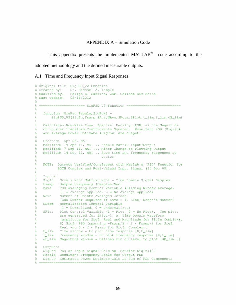
69
APPENDIX A – Simulation Code
This appendix presents the implemented MATLAB code according to the
adopted methodology and the defined measurable outputs.
A.1 Time and Frequency Input Signal Responses
% Original file: SigPSD_V2 Function % Created by: Dr. Michael A. Temple % Modified by: Felipe E. Garrido, CAP. Chilean Air Force % Last update: 02/16/2012 % % ====================== SigPSD_V3 Function ========================== % % function [SigPsd,Fscale,SigPow] = % SigPSD_V3(SigIn,Fsamp,SAve,NAve,SNorm,SPlot,t_lim,f_lim,dB_lim) % % Calculates Row-Wise Power Spectral Density (PSD) as the Magnitude % of Fourier Transform Coefficients Squared. Resultant PSD (SigPsd) % and Average Power Estimate (SigPow) are output. % % Created: Apr 06, MAT % Modified: 19 Apr 11, MAT .. Enable Matrix Input/Output % Modified: 7 Sep 11, MAT ... Minor Change to Plotting Output % Modified: 14 Dec 11, MAT .. Save time and frequency responses as % vector. % % NOTE: Outputs Verified/Consistent with Matlab's 'PSD' Function for % BOTH Complex and Real-Valued Input Signal (10 Dec 08). % % Inputs: % SigIn Nrow x NCol Matrix: NCol = Time Domain Signal Samples % Fsamp Sample Frequency (Samples/Sec) % SAve PSD Averaging Control Variable (Sliding Window Average) % (1 = Average Applied, 0 = No Average Applied) % NAve Number of Points Averaged Across % (Odd Number Required if Save = 1, Else, Doesn't Matter) % SNorm Normalization Control Variable % (1 = Normalized, 0 = UnNormalized) % SPlot Plot Control Variable (1 = Plot, 0 = No Plot). Two plots % are generated for SPlot=1: A) Time Domain Waveform % (amplitude for SigIn Real and Magnitude for SigIn Complex), % B) SigIn PSD (spanning -Fsamp/2 < f < Fsamp/2 for SigIn % Real and 0 < f < Fsamp for SigIn Complex). % t_lim Time window = to plot time response [0,t_lim] % f_lim Frequency window = to plot frequency response [0,f_lim] % dB_lim Magnitude window = Defines min dB level to plot [dB_lim,0] % % Outputs: % SigPsd PSD of Input Signal Calc as |Fourier{SigIn}|^2 % Fscale Resultant Frequency Scale for Output PSD % SigPow Estimated Power Estimate Calc as Sum of PSD Components % ====================================================================

70
function [SigPsd,Fscale,SigPow] = SigPSD_V3(SigIn,Fsamp,SAve,NAve,SNorm,SPlot,t_lim,f_lim,dB_lim) [NrowIn,NcolIn]=size(SigIn); if NcolIn==1 % Column Vector Input Transpose & Process as Row Vector SigIn=SigIn.'; [Nrow,Ncol]=size(SigIn); else Nrow=NrowIn; Ncol=NcolIn; end SigVal = isreal(SigIn(1,1)); % SigVal=1 (Real) or SigVal=0 (Complex) SigFFT=(fft(real(SigIn.')).'/Ncol); SigPsd=abs(SigFFT).^2; % Non-Shifted PSD SigPow=sum(SigPsd.'); if(SAve==1) % Apply Row-Wise Averaging/Smoothing to PSD NTest = mod(NAve,2); % Check/Adjust NAve to be an Odd Number if NTest==0 % Even NAve Input NAve=NAve+1; % Adjust NAve to be Odd end; for j=1:Nrow %TmpPsd=SigPsd(j,:); SigPsd(j,:)=smooth(SigPsd(j,:),NAve); end end PSDmax=max(SigPsd.'); PSDfloor=PSDmax/10000; % Set PSD Floor Level to -40 dB Below Max Value for j=1:Nrow % Threshold / Set PSD Floor Values for k=1:Ncol if SigPsd(j,k)<PSDfloor(j) SigPsd(j,k)=PSDfloor(j); end end end PSDmax=max(SigPsd.'); % Update PSDmax if SNorm==1 % Normalize PSD if Selected SigPsd=SigPsd./repmat(PSDmax.',1,Ncol); end if NcolIn==1 % Return Output to Column Vector SigPsd=SigPsd.'; end delf=Fsamp/(Ncol-1); % Freq Plot Step Size Fscale=0:delf:(Ncol-1)*delf; % Output PSD Freq Scale if SPlot==1 % Produce Output Plots disp(' ') disp('Generating Plot') disp(' ')

71
if (Nrow==1||Ncol==1 ) SigPlot=(abs(SigIn)).^2; SigPlot=SigPlot/max(SigPlot); PsdPlot=SigPsd; else % Use 1st Row of SigIn & SigPsd Matrix for Plot Default SigPlot=(abs(SigIn(1,:))).^2; PsdPlot=SigPsd(1,:); end figure subplot(2,1,1) % Top Time Plot tscale=linspace(0,Ncol/Fsamp,Ncol); SigPlot_dB=10*log10(SigPlot); if SigVal==1 % SigIn is Real plot(tscale,SigPlot_dB); grid; set(gca,'XLim',[0 t_lim]); set(gca,'YLim',[dB_lim 0]); xlabel('Time [s]') ylabel('Magnitude') else % SigIn is Complex ... Plot Amplitude as Abs(SigIn) plot(tscale,SigPlot_dB); grid; set(gca,'XLim',[0 t_lim]); set(gca,'YLim',[dB_lim 0]); xlabel('Time [s]') ylabel('Magnitude') end save('Time_response','SigPlot_dB','tscale'); subplot(2,1,2) % Select Middle PSD Figure if SigVal==1 % SigIn Real: Plot FFTshift{PSD} for -Fs/2 < f < Fs/2 fpos=(0:delf:delf*(ceil(Ncol/2)-1)); fneg= -fliplr( (delf:delf:delf*(Ncol-ceil(Ncol/2))) ); FrqPlot=[fneg fpos]; FrqPlot_dB=10*log10(fftshift(PsdPlot)); plot(FrqPlot,FrqPlot_dB); % PSD Shifted else % SigIn Complex: Plot PSD for 0 < f < Fsamp FrqPlot=0:delf:(Ncol-1)*delf; FrqPlot_dB=10*log10(PsdPlot); plot(FrqPlot, FrqPlot_dB); % FFT Shifted end save('PSD_signal','FrqPlot_dB','FrqPlot'); % Adjust X & Y Axis Limits set(gca,'YLim',[dB_lim 0]); set(gca,'XLim',[0 f_lim]); xlabel('Frequency [Hz]') ylabel('| FFT |^ 2') grid end % ====================== End SigPSD_V3 Function=======================

72
A.2 QMFB Process Code
% QMFB PROCESS % Original file: qmfb.m % Created by : Phillip E. Pace % Modified by : Felipe Garrido, CAP. Chilean Air Force. % Last update : 02/02/2012. % This code is used to create the layers and the neccesary output data % to processing them according to the desired time-frequency plot % This code call the function tsinc.m that creates de coefficients % according to the especified filter created for Phillip E. Pace. %%%%%%%%%%%%%%%%%%%%%%%%%%%%%%%%%%%%%%%%%%%%%%%%%%%%%%%%%%%%%%%%%%%%%%%%%%%%% clear all close all tic % Files Loading load preamble_res_10000_25.mat % -- Input data -- c0=[preamble_res_10000_25]'; % Input signal padded with zeros [d1, c1] = tsinc(c0); % Sinc Modified Filter function % -- Number of Layers to Compute -- f=c0; % Input signal n = floor(log2(length(f))); % Determine the amount of layers from the length of the signal N = n; % number of layers % -- Formatting the Signal -- (to pass the signal through the filter bank) I(1:2^n,1) = f(1:2^n); out = I; % -- Generating the Output Layers -- % Decompose the function W = waitbar(0,'Computing Layers...'); for lay = 1:N % layer %disp(lay) % Show what layer is been generated waitbar(lay/(N+1),W) flag = 1; % Flag used to set up the columns in the output matrix % Reshape the output matrix [r,c] = size(out); out = zeros(r./2, c.*2); for i = 1:2 ^(lay-1) % column of I (low to high) [G,H] = tsinc(I(:,i)); % Evaluate the filter (sinc modified) % over the signal going by columns % Setting the output matrix (Layer) by High Pass (G) and Low Pass (H) filtering output if flag out(:, i.*2-1) = H; % Low Pass Branch of QMFB Tree out(:, i.*2) = G; % High Pass Branch of QMFB Tree else out(:, i.*2-1) = G; % High Pass Branch of QMFB Tree out(:, i.*2) = H; % Low Pass Branch of QMFB Tree end; flag = ~flag; % Change in the flag value end; % Output Matrix and data to work with
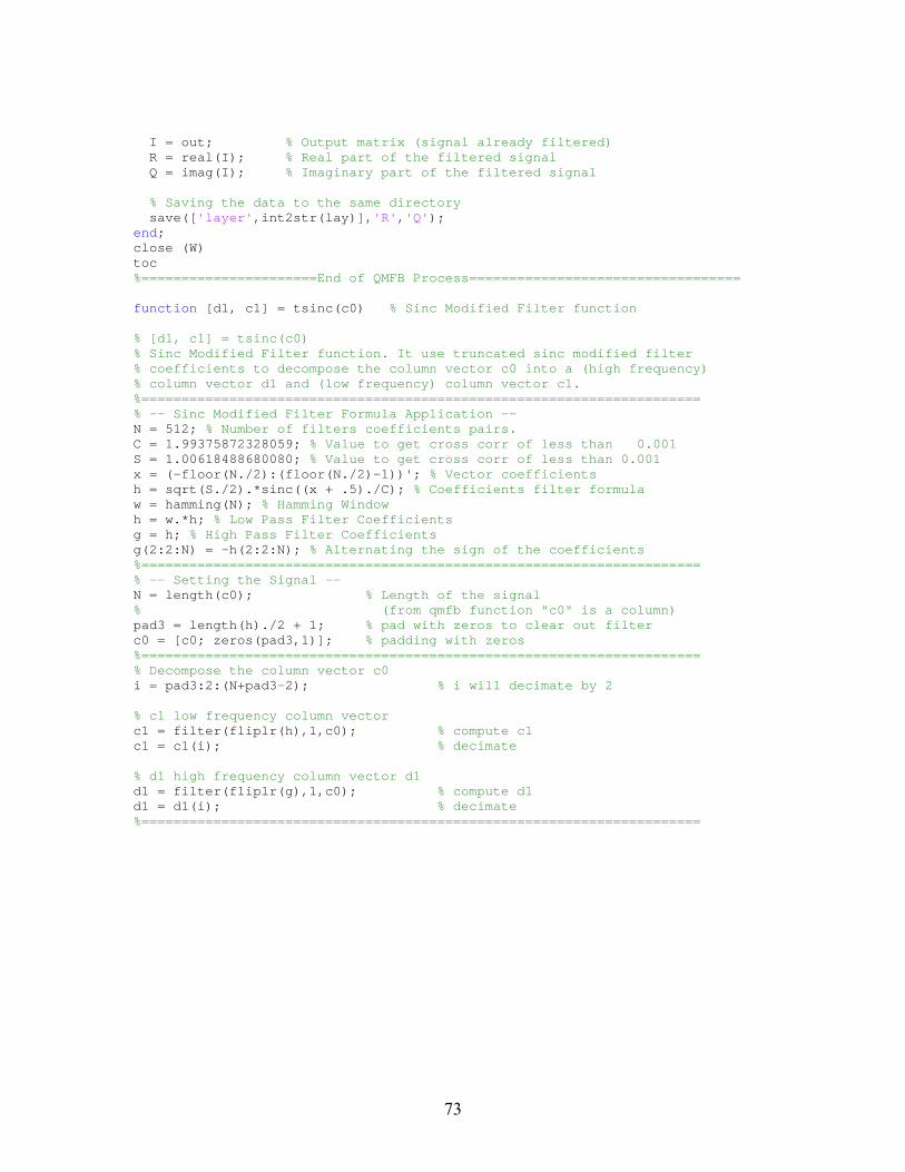
73
I = out; % Output matrix (signal already filtered) R = real(I); % Real part of the filtered signal Q = imag(I); % Imaginary part of the filtered signal % Saving the data to the same directory save(['layer',int2str(lay)],'R','Q'); end; close (W) toc %======================End of QMFB Process================================== function [d1, c1] = tsinc(c0) % Sinc Modified Filter function % [d1, c1] = tsinc(c0) % Sinc Modified Filter function. It use truncated sinc modified filter % coefficients to decompose the column vector c0 into a (high frequency) % column vector d1 and (low frequency) column vector c1. %====================================================================== % -- Sinc Modified Filter Formula Application -- N = 512; % Number of filters coefficients pairs. C = 1.99375872328059; % Value to get cross corr of less than 0.001 S = 1.00618488680080; % Value to get cross corr of less than 0.001 x = (-floor(N./2):(floor(N./2)-1))'; % Vector coefficients h = sqrt(S./2).*sinc((x + .5)./C); % Coefficients filter formula w = hamming(N); % Hamming Window h = w.*h; % Low Pass Filter Coefficients g = h; % High Pass Filter Coefficients g(2:2:N) = -h(2:2:N); % Alternating the sign of the coefficients %====================================================================== % -- Setting the Signal -- N = length(c0); % Length of the signal % (from qmfb function "c0" is a column) pad3 = length(h)./2 + 1; % pad with zeros to clear out filter c0 = [c0; zeros(pad3,1)]; % padding with zeros %====================================================================== % Decompose the column vector c0 i = pad3:2:(N+pad3-2); % i will decimate by 2 % c1 low frequency column vector c1 = filter(fliplr(h),1,c0); % compute c1 c1 = c1(i); % decimate % d1 high frequency column vector d1 d1 = filter(fliplr(g),1,c0); % compute d1 d1 = d1(i); % decimate %======================================================================

74
A.3 QN Matrix Generation Code
% Qn Matrix generation and Plotting % Original file : qmfb.m % Created by : Phillip E. Pace % modified by : Capt Felipe E. Garrido 01/04/2012 % Last update : 02/16/2012 %%%%%%%%%%%%%%%%%%%%%%%%%%%%%%%%%%%%%%%%%%%%%%%%%%%%%%%%%%%%%%%%%%% % This code allows to choose which layers do you want to plot % and save the matrix with useful data as Q_xx.mat,xx= layer number % % Input variables are the following: % L= lower layer to plot (Min layer=1) % H= higher layer to plot (Max layer= N) % fs= Sampling frequency of the input data (Fsamp_XX) % freq_limit= max frequency in window % Time_limit= max time in window %%%%%%%%%%%%%%%%%%%%%%%%%%%%%%%%%%%%%%%%%%%%%%%%%%%%%%%%%%%%%%%%%%% clear all close all %% Warning: % Check you are loading the correct data file load preamble_res_10000_25.mat; %% Set the appropiate parameters fs=Fsamp_10000; % Sample frequency according to the % resampled data L=2; % Lower layer to plot H=24; % Higher layer to plot freq_limit=9e6; % Y axis limit Time_limit=2.5e-5; % X axis limit %% Plotting for yy=L:H load (['layer',num2str(yy),'.mat']); % Formating the Layer layer = abs(R + 1i*Q); % absolute value of the layer layer = (layer/max(max(layer))).^2;% Normalizing the layer M = layer; % Set values to dB [m,n]=size(M); % Set axis sizes T=1/fs; % Sampling period f=linspace(0,fs/2,n); % Setting the frequency axis NUM_SAMPLES = m*n; % Length of the new signal time=linspace(0,NUM_SAMPLES*T,m); % Setting the time axis dt=(NUM_SAMPLES*T)/(m-1); % delta t df=(fs/(2*(n-1))); % delta f t_max=ceil(Time_limit/dt)+1; f_max=ceil(freq_limit/df)+1; new_Q=(M(1:(t_max),1:(f_max))).'; new_layer=(R(1:(t_max),1:(f_max)) + 1i*Q(1:(t_max),1:(f_max))).'; n_t=time(1:t_max); n_f=f(1:f_max); Q_dB=10*log10(new_Q.^2);

75
clear layer; % clear current layer matrix from the workspace % Color Plots figure; %pcolor(time(1:t_max),f(1:f_max),Q_dB') pcolor(n_t,n_f,Q_dB) % title(['"Time - Frequency Plane Layer ',... % num2str(yy),' with \Deltat=',num2str(dt),... % ' and \Deltaf=',num2str(df),'"']) xlabel('Time [s]'),ylabel('Frequency [Hz]') colorbar,colormap(jet) caxis([-30,0]) shading interp % figure; % %pcolor(time(1:t_max),f(1:f_max),Q_dB') % pcolor(n_t,n_f,Q_dB) % % title(['"Time - Frequency Plane Layer ',... % % num2str(yy),' with \Deltat=',num2str(dt),... % % ' and \Deltaf=',num2str(df),'"']) % xlabel('Time [sec]'),ylabel('Frequency [Hz]') % colorbar,colormap(jet) % caxis([-30,0]) % shading flat save(['Q_',int2str(yy)],'Q_dB','new_Q','time','f','dt','df',... 'fs','t_max','f_max','new_layer'); end

76
A.4 Input/Output Frequency-Time (F-T) Analysis Code
% TIME AND FREQUENCY ANALYSIS % % Created by : Felipe E. Garrido, CAP. Chilean Air Force % Last update : 02/16/2012 % % This code computes and save Normalized Average Time % and Normalized Average frequency vector for a given layer % %%%%%%%%%%%%%%%%%%%%%%%%%%%%%%%%%%%%%%%%%%%%%%%%%%%%%%%%%%%%%%%%%%%%%%% %% Warning % 1.- The file Layer_plotting, must be run before running this code to % generate a given Q_XX.mat file. % %%%%%%%%%%%%%%%%%%%%%%%%%%%%%%%%%%%%%%%%%%%%%%%%%%%%%%%%%%%%%%%%%%%%%%% %% % Input variables are the following: % layer = number of the layer you want to plot (Min layer=1) % sel = variable to choose between time or frequency % Choose: % Time plot ===> sel=1 % Frequency plot ===> sel=2 % %%%%%%%%%%%%%%%%%%%%%%%%%%%%%%%%%%%%%%%%%%%%%%%%%%%%%%%%%%%%%%%%%%%%%%% clear all close all layer=13; % Choose the layer to plot load (['Q_',num2str(layer),'.mat']); sel=1; % Time plot=1, Frequency plot=2 % n_t=time(1:t_max); % n_f=f(1:f_max); % Q_dB=10*log10(new_Q.^2); if sel==1; t=mean(new_Q,1); t2=t/max(t); t2_dB=10*log10(t2(1:t_max)); tt=time(1:t_max); figure; plot(tt,t2_dB) % title(['"Normalized Average Time plot for Layer ',... % num2str(layer),' with \Deltat=',num2str(dt),'"']) %xlabel('Time [s]') ylabel('dB') ylim([-30 0]) xlim([0 Time_limit]) grid on save(['ave_t_',int2str(layer)],'t2_dB','tt'); elseif sel==2; nf=mean(new_Q,2); f2=nf/max(nf);

77
f2_dB=10*log10(f2(1:f_max)); w=f(1:f_max); figure; plot(f2_dB,w) % title(['"Normalized Average frequency plot for Layer ',... % num2str(layer),' with \Deltaf=',num2str(df),'"']) %ylabel('Frequency [Hz]') xlabel('dB') xlim([-30 0]) ylim([0 freq_limit]) grid on save(['ave_f_',int2str(layer)],'f2_dB','w'); else disp('ERROR:') disp('Choose: 1=Plot Average Time or 2=Plot Average Frequency') end %=====================End of Time/Frequency analysis code==================== % OVERLAY FREQUENCY RESPONSE PLOT % % Created by : Felipe E. Garrido, CAP. Chilean Air Force % Last update : 02/16/2012 % % This code computes overlay frequency response according to input % signal and two chosen layers % %%%%%%%%%%%%%%%%%%%%%%%%%%%%%%%%%%%%%%%%%%%%%%%%%%%%%%%%%%%%%%%%%%%%%%% % Input variables are the following: % PSD_signal.mat = initial signal frequency response % ave_f_20.mat = single burst frequency response % ave_f_19.mat = burst integration frequency response %%%%%%%%%%%%%%%%%%%%%%%%%%%%%%%%%%%%%%%%%%%%%%%%%%%%%%%%%%%%%%%%%%%%%%% clear all close all load PSD_signal.mat figure plot (FrqPlot,FrqPlot_dB,'b') hold on load ave_f_20.mat plot(w,f2_dB,'r') hold on load ave_f_19.mat plot(w,f2_dB,'k') grid on legend('Input','Single Burst','Burst Integration','location','South') xlim([0 2e6]) ylim([-30 0]) xlabel('Frequency [Hz]') ylabel('Magnitude [dB]') %=====================End of Overlay FREQUENCY response======================

78
% OVERLAY TIME RESPONSE PLOT % % Created by : Felipe E. Garrido, CAP. Chilean Air Force % Last update : 02/16/2012 % % This code computes overlay frequency response according to input % signal and two chosen layers % %%%%%%%%%%%%%%%%%%%%%%%%%%%%%%%%%%%%%%%%%%%%%%%%%%%%%%%%%%%%%%%%%%%%%%% % Input variables are the following: % Time_response.mat = initial signal frequency response % ave_t_13.mat = single burst frequency response % ave_t_12.mat = burst integration frequency response %%%%%%%%%%%%%%%%%%%%%%%%%%%%%%%%%%%%%%%%%%%%%%%%%%%%%%%%%%%%%%%%%%%%%%% clear all close all load Time_response.mat figure plot (tscale,SigPlot_dB,'b') hold on load ave_t_13.mat plot(tt,t2_dB,'r') hold on load ave_t_12.mat plot(tt,t2_dB,'k') grid on legend('Input','Single Burst','Burst Integration','location','south') xlim([0 0.1e-3]) ylim([-30 0]) xlabel('Time [s]') ylabel('Magnitude [dB]') %=====================End of Overlay TIME response======================

79
APPENDIX B – QMFB Outputs for 802.11a Wi-Fi Preamble Signal
This appendix presents a complete set of available layer outputs (QN) for the 802.11a
signal analyzed in Section 4.2 according to computed QMFB outputs.
QMFB Layer Q3
QMFB Layer Q5
QMFB Layer Q2
QMFB Layer Q4

80
QMFB Layer Q7
QMFB Layer Q9
QMFB Layer Q11
QMFB Layer Q6
QMFB Layer Q8
QMFB Layer Q10
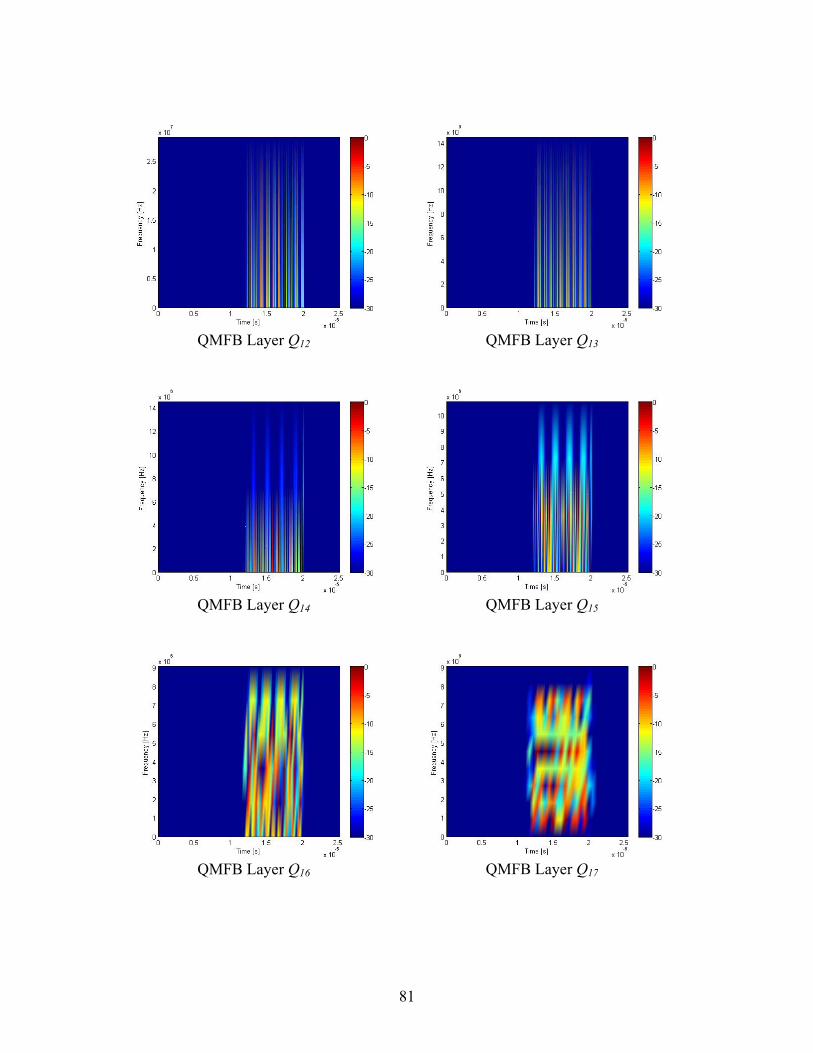
81
QMFB Layer Q13
QMFB Layer Q15
QMFB Layer Q17
QMFB Layer Q12
QMFB Layer Q14
QMFB Layer Q16

82
QMFB Layer Q19
QMFB Layer Q21
QMFB Layer Q23
QMFB Layer Q18
QMFB Layer Q20
QMFB Layer Q22
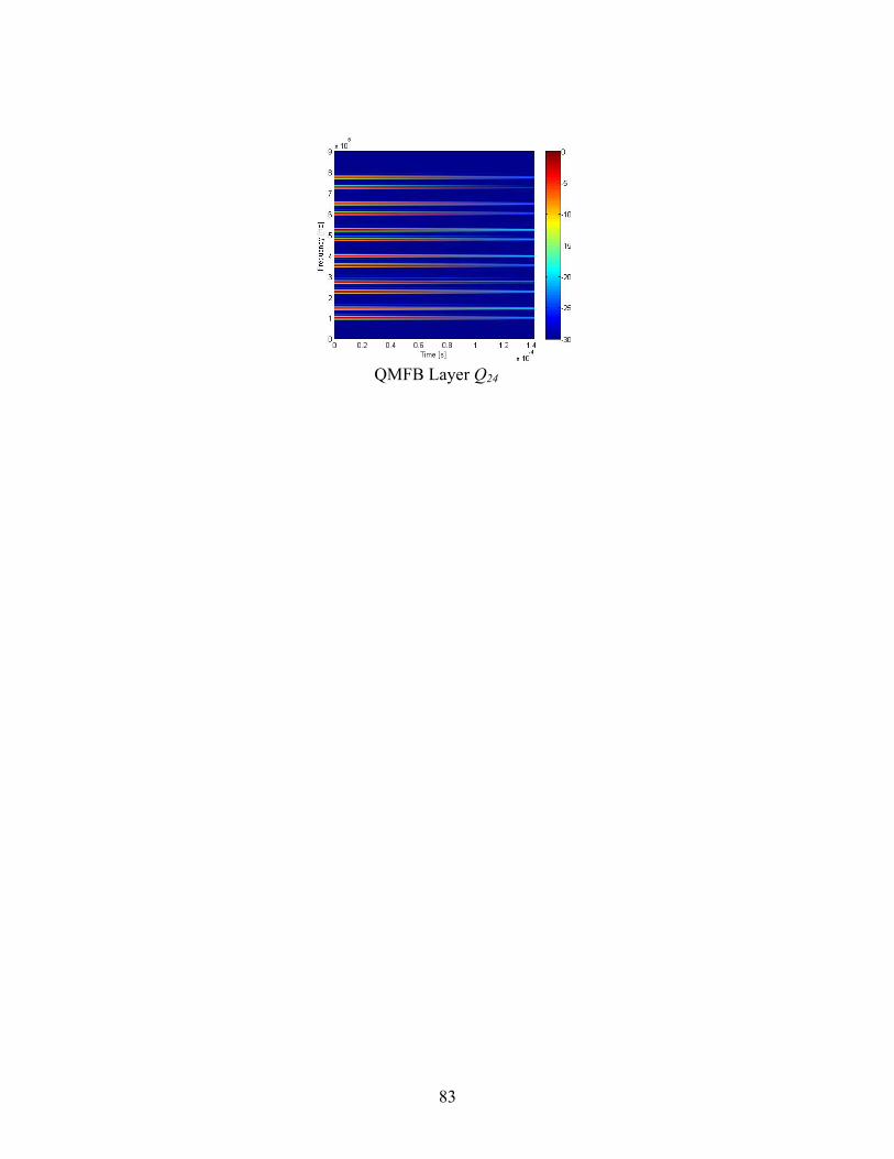
83
QMFB Layer Q24

84
APPENDIX C. Time (Δt) and Frequency (Δf) Resolution Tables
C.1 802.11a Wi-Fi Signal: Preamble Only (Section 4.2.1)
Sampling Frequency
fs [Hz] fs = 5.94x10¹⁰ fs = 1.19x10¹¹ fs = 2.38 x10¹¹
Layer
#
Δf
[Hz]
Δt
[s]
Δf
[Hz]
Δt
[s]
Δf
[Hz]
Δt
[s]
6 4.71x10⁸ 1.08x10⁻⁹ 9.43x10⁸ 5.39x10⁻¹⁰ 1.89x10⁹ 2.70x10⁻¹⁰
7 2.33x10⁸ 2.16x10⁻⁹ 4.68x10⁸ 1.08x10⁻⁹ 9.35x10⁸ 5.39x10⁻¹⁰
8 1.16x10⁸ 4.31x10⁻⁹ 2.33x10⁸ 2.16x10⁻⁹ 4.66x10⁸ 1.08x10⁻⁹
9 5.81x10⁷ 8.62x10⁻⁹ 1.16x10⁸ 4.31x10⁻⁹ 2.32x10⁸ 2.16x10⁻⁹
10 2.90x10⁷ 1.73x10⁻⁸ 5.80x10⁷ 8.62x10⁻⁹ 1.16x10⁸ 4.31x10⁻⁹
11 1.45x10⁷ 3.45x10⁻⁸ 2.90x10⁷ 1.73x10⁻⁸ 5.80x10⁷ 8.62x10⁻⁹
12 7.25x10⁶ 6.90x10⁻⁸ 1.45x10⁷ 3.45x10⁻⁸ 2.90x10⁷ 1.73x10⁻⁸
13 3.62x10⁶ 1.38x10⁻⁷ 7.25x10⁶ 6.90x10⁻⁸ 1.45x10⁷ 3.45x10⁻⁸
14 1.81x10⁶ 2.76x10⁻⁷ 3.62x10⁶ 1.38x10⁻⁷ 7.25x10⁶ 6.90x10⁻⁸
15 9.06x10⁵ 5.52x10⁻⁷ 1.81x10⁶ 2.76x10⁻⁷ 3.62x10⁶ 1.38x10⁻⁷
16 4.53x10⁵ 1.11x10⁻⁶ 9.06x10⁵ 5.53x10⁻⁷ 1.81x10⁶ 2.77x10⁻⁷
17 2.27x10⁵ 2.22x10⁻⁶ 4.53x10⁵ 1.11x10⁻⁶ 9.06x10⁵ 5.56x10⁻⁷
18 1.13x10⁵ 4.45x10⁻⁶ 2.26x10⁵ 2.23x10⁻⁶ 4.53x10⁵ 1.11x10⁻⁶
19 5.66x10⁴ 8.97x10⁻⁶ 1.13x10⁵ 4.49x10⁻⁶ 2.27x10⁵ 2.25x10⁻⁶
20 2.83x10⁴ 1.82x10⁻⁵ 5.66x10⁴ 9.12x10⁻⁶ 1.13x10⁵ 4.56x10⁻⁶
21 1.42x10⁴ 3.77x10⁻⁵ 2.83x10⁴ 1.88x10⁻⁵ 5.66x10⁴ 9.42x10⁻⁶

85
C.2 802.11a Wi-Fi Signal: Complete Burst (Section 4.2.2)
Sampling Frequency
fs [Hz] fs = 2.38x10¹⁰ fs = 5.94 x10¹⁰ fs = 1.31 x10¹¹
Layer
#
Δf
[Hz]
Δt
[s]
Δf
[Hz]
Δt
[s]
Δf
[Hz]
Δt
[s]
6 1.88x10⁸ 2.69x10⁻⁹ 4.71x10⁸ 1.08x10⁻⁹ 1.04x10⁹ 4.90x10⁻¹⁰
7 9.35x10⁷ 5.39x10⁻⁹ 2.33x10⁸ 2.16x10⁻⁹ 5.14x10⁸ 9.80x10⁻¹⁰
8 4.66x10⁷ 1.08x10⁻⁸ 1.16x10⁸ 4.31x10⁻⁹ 2.56x10⁸ 1.96x10⁻⁹
9 2.32x10⁷ 2.16x10⁻⁸ 5.81x10⁷ 8.62x10⁻⁹ 1.27x10⁸ 3.92x10⁻⁹
10 1.15x10⁷ 4.31x10⁻⁸ 2.90x10⁷ 1.73x10⁻⁸ 6.38x10⁷ 7.84x10⁻⁹
11 5.80x10⁶ 8.63x10⁻⁸ 1.45x10⁷ 3.45x10⁻⁸ 3.19x10⁷ 1.57x10⁻⁸
12 2.89x10⁶ 1.73x10⁻⁷ 7.25x10⁶ 6.90x10⁻⁸ 1.59x10⁷ 3.14x10⁻⁸
13 1.44x10⁶ 3.45x10⁻⁷ 3.62x10⁶ 1.38x10⁻⁷ 7.97x10⁶ 6.27x10⁻⁸
14 7.25x10⁵ 6.93x10⁻⁷ 1.81x10⁶ 2.76x10⁻⁷ 3.99x10⁶ 1.25x10⁻⁷
15 3.62x10⁶ 1.39x10⁻⁶ 9.06x10⁵ 5.52x10⁻⁷ 1.99x10⁶ 2.51x10⁻⁷
16 1.81x10⁵ 2.80x10⁻⁶ 4.53x10⁵ 1.11x10⁻⁶ 9.97x10⁶ 5.03x10⁻⁷
17 9.06x10⁴ 5.70x10⁻⁶ 2.27x10⁵ 2.22x10⁻⁶ 4.98x10⁵ 1.01x10⁻⁶
18 4.53x10⁴ 1.18x10⁻⁵ 1.13x10⁵ 4.45x10⁻⁶ 2.49x10⁵ 2.02x10⁻⁶
19 2.26x10⁴ 2.52x10⁻⁵ 5.66x10⁴ 8.97x10⁻⁶ 1.25x10⁵ 4.08x10⁻⁶
20 1.13x10⁴ 5.89x10⁻⁵ 2.83x10⁴ 1.82x10⁻⁵ 6.23x10⁴ 8.29x10⁻⁶
21 5.63x10³ 1.21x10⁻⁴ 1.42x10⁴ 3.77x10⁻⁵ 3.11x10⁴ 1.71x10⁻⁵

86
C.3 802.16e WiMAX Signal
Sampling Frequency
fs [Hz]
Both Modes
fs = 1.19x10⁹
Data-Only
fs = 1.18x10¹⁰
Range-Only
fs = 3.56 x10¹⁰
Layer
#
Δf
[Hz]
Δt
[s]
Δf
[Hz]
Δt
[s]
Δf
[Hz]
Δt
[s]
6 9.42x10⁶ 5.39x10⁻⁸ 9.42x10⁷ 5.39x10⁻⁹ 2.83x10⁸ 1.80x10⁻⁹
7 4.68x10⁶ 1.08x10⁻⁷ 4.68x10⁷ 1.08x10⁻⁸ 1.40x10⁸ 3.59x10⁻⁹
8 2.32x10⁶ 2.16x10⁻⁷ 3.33x10⁷ 2.16x10⁻⁸ 6.99x10⁷ 7.19x10⁻⁹
9 1.15x10⁶ 4.31x10⁻⁷ 1.16x10⁷ 4.31x10⁻⁸ 3.49x10⁷ 1.44x10⁻⁸
10 5.80x10⁵ 8.62x10⁻⁷ 5.80x10⁶ 8.62x10⁻⁸ 1.74x10⁷ 2.87x10⁻⁸
11 2.90x10⁵ 1.72x10⁻⁶ 2.90x10⁶ 1.72x10⁻⁷ 8.70x10⁶ 5.75x10⁻⁸
12 1.45x10⁵ 3.45x10⁻⁶ 1.45x10⁶ 3.45x10⁻⁷ 4.34x10⁶ 1.15x10⁻⁷
13 7.24x10⁴ 6.90x10⁻⁶ 7.25x10⁵ 6.90x10⁻⁷ 2.16x10⁶ 2.31x10⁻⁷
14 3.62x10⁴ 1.38x10⁻⁵ 3.62x10⁵ 1.38x10⁻⁶ 1.09x10⁶ 4.60x10⁻⁷
15 1.81x10⁴ 2.76x10⁻⁵ 1.81x10⁵ 2.76x10⁻⁶ 5.44x10⁵ 9.21x10⁻⁷
16 9.06x10³ 5.53x10⁻⁵ 9.06x10⁴ 5.53x10⁻⁶ 2.71x10⁵ 1.84x10⁻⁶
17 4.53x10³ 1.11x10⁻⁴ 4.53x10⁴ 1.11x10⁻⁵ 1.36x10⁵ 3.69x10⁻⁶
18 2.27x10³ 2.33x10⁻⁴ 2.27x10⁴ 2.22x10⁻⁵ 6.80x10⁴ 7.42x10⁻⁶
19 1.13x10² 4.75x10⁻⁴ 1.13x10⁴ 4.45x10⁻⁵ 3.39x10⁴ 1.50x10⁻⁵
20 5.63x101 1.02x10⁻³ 5.66x10³ 8.97x10⁻⁵ 1.69x10⁴ 3.03x10⁻⁵
21 2.84x101 2.11x10⁻³ 2.83x10³ 1.82x10⁻⁴ 8.58x10³ 6.04x10⁻⁵

87
Bibliography
1. Pace, P. E. Detecting and Classifying Low Probability of Intercept Radar. Artech House, Boston, second edition, 2008. ISBN 978-1-59693-234.
2. Skelar, B. Digital Communications Fundamentals and Applications.
Prentice Hall PTR, New Jersey, Second Edition, 2008. ISBN 0-13-084788-7.
3. Jarpa, P. Quantifying the Differences in Low Probability of
Intercept Radar Waveforms Using Quadrature Mirror Filtering. Master’s thesis, Naval Postgraduate School, Monterrey, CA, September 2002.
4. Atienza, D. V. Characterization of Noise Technology Radar (NTR) Signal Detectability Using Non-Cooperative Receiver. Master’s thesis, Air Force Institute of Technology, GE-ENG-11-01, March 2011.
5. Gronholz, B. D. Non-Cooperative Detection of Ultra Wideband
Signals. Master’s thesis, Air Force Institute of Technology, GE-ENG-04-29, March 2004.
6. Mims, W. H. Wideband Signal Detection Using a Down-Converting
Channelized Receiver. Master’s thesis, Air Force Institute of Technology, GE-ENG-06-42, March 2006.
7. Szmajda, M, K. Gorecki and J. Mroczka, “Gabor Transform,
Gabor-Wigner Transform and SPWVD as Time-Frequency Analysis of Power Quality. Int’l Conf on Harmonics and Quality of Power (ICHQP2010), Bergamo, Italy, Sep 2010.
8. Klein, R. W. ., M. A. Temple and M. J. Mendenhall, “Application
of Wavelet-Based RF Fingerprinting to enhance wireless network security”, Jour of Communications and Networks, Vol. 11, No. 6, Dec 2009.
9. IEEE 802.11-2005, Local and Metropolitan Area Networks, Part
11: Wireless LAN Medium Access Control (MAC) and Physical Layer (PHY) specifications. Inst of Electrical and Electronics Engineers, New York, New York, USA, Aug 2005.

88
10. Reising, D. R., M. A. Temple and M. E. Oxley, “Gabor-Based RF-DNA Fingerprinting for Classifying 802.16e WiMAX Mobile Subscribers”. Int’l Conf on Computing, Networking and Communications (ICNC12), Maui, Hawaii, Jan 2012.
11. Reising, D. R. and M. A. Temple, “WiMAX Mobile Subscriber
Verification Using Gabor-Based RF-DNA Fingerprints”, Int’l Communications Conference (ICC12), Ottawa, Canada, Jun 2012.
12. IEEE Std 802.16e-2005, Local and Metropolitan Area Networks,
Part 16: Air Interface for Broadband Wireless Access System. Inst of Electrical and Electronics Engineers, New York, New York, USA, Feb 2006. ISBN 0-7381-4857-1.
13. BreezeMAX Extreme 5000: WiMAX 16e Pioneer for the License-
Exempt Market, Alvarion, Edition 215373 Rev. A, 2009.

REPORT DOCUMENTATION PAGE Form Approved
OMB No. 0704-0188 Public reporting burden for this collection of information is estimated to average 1 hour per response, including the time for reviewing instructions, searching existing data sources, gathering and maintaining the data needed, and completing and reviewing this collection of information. Send comments regarding this burden estimate or any other aspect of this collection of information, including suggestions for reducing this burden to Department of Defense, Washington Headquarters Services, Directorate for Information Operations and Reports (0704-0188), 1215 Jefferson Davis Highway, Suite 1204, Arlington, VA 22202-4302. Respondents should be aware that notwithstanding any other provision of law, no person shall be subject to any penalty for failing to comply with a collection of information if it does not display a currently valid OMB control number. PLEASE DO NOT RETURN YOUR FORM TO THE ABOVE ADDRESS.
1. REPORT DATE (DD-MM-YYYY)
22/03/2012
2. REPORT TYPE
Master’s Thesis
3. DATES COVERED (From - To)
Aug 2010-Mar 2012
4. TITLE AND SUBTITLE
OFDM-BASED SIGNAL EXPLOTATION USING QUADRATURE MIRROR FILTER BANK (QMFB) PROCESSING
5a. CONTRACT NUMBER
5b. GRANT NUMBER
5c. PROGRAM ELEMENT NUMBER
6. AUTHOR(S) Garrido, Felipe E., Captain, Chilean Air Force
5d. PROJECT NUMBER
5e. TASK NUMBER
5f. WORK UNIT NUMBER
7. PERFORMING ORGANIZATION NAME(S) AND ADDRESS(ES) AND ADDRESS(ES)
Air Force Institute of Technology Graduate School of Engineering and Management (AFIT/ENG) 2950 Hobson Way WPAFB OH 45433-7765
8. PERFORMING ORGANIZATION REPORT NUMBER
AFIT/GE/ENG/12-16
9. SPONSORING / MONITORING AGENCY NAME(S) AND ADDRESS(ES) Letnic, Dalibor, Lt Col, Chilean Air Force Chilean Air Force Mission 1100 17th Street N.W., Suite 900 Washington, D.C. 20036 (202)872-1335 x201
10. SPONSOR/MONITOR’S ACRONYM(S)
11. SPONSOR/MONITOR’S REPORT NUMBER(S)
12. DISTRIBUTION / AVAILABILITY STATEMENT APPROVED FOR PUBLIC RELEASE; DISTRIBUTION UNLIMITED
13. SUPPLEMENTARY NOTES
This material is declared a work of the U.S. Government and is not subject to copyright protection in the United States. 14. ABSTRACT By performing QMFB processing with a given signal it is possible to obtain Frequency-Time (F-T) outputs that represent signal features such as bandwidth (W), center frequency (fc), signal duration (Ts), modulation type (AM, FM, BPSK, QAM, etc), frequency content and time allocation. Because of its unique structure, two widely used signals based on Orthogonal Frequency Division Multiplexing (OFDM) were chosen as signals of interest for demonstration. The general implementation of the QMFB process is described along with the basic structure of OFDM signals related to the physical layer perspective of 802.11a Wi-Fi and 802.16e WiMAX frame structures are described. The adopted methodology is aimed at exploiting signal of interest features accounting for the effects of signal resampling and zero-padding. Computed simulation results are obtained after applying the defined methodology to each signal of interest. Initial time domain and frequency domain responses are presented for each input signal along with the initial and computed resampled parameters for each case. Results for selected QMFB outputs are presented using 2D F-T QMFB plots and 1D average frequency and average time plots. These plots enable qualitative visual assessment such as may be used by a human operator. The 1D responses are computed for the input signal and output QMFB responses and compared using overlay plots for single burst and multiple integrated burst inputs. Resultant time (Δt) and frequency (Δf) resolutions were consistent and validate the usefulness of QMFB processing.
15. SUBJECT TERMS QMFB, OFDM, 802.11a Wi-Fi, 802.16e WiMAX
16. SECURITY CLASSIFICATION OF: 17. LIMITATION OF ABSTRACT
18. NUMBER OF PAGES
19a. NAME OF RESPONSIBLE PERSON Dr. Michael A. Temple
a. REPORT U
b. ABSTRACT U
c. THIS PAGE U
UU 104
19b. TELEPHONE NUMBER (include area code) 937-255-3636 x4279, [email protected]
Standard Form 298 (Rev. 8-98) Prescribed by ANSI Std. Z39.18


