

Optimal Combination of Multiple Atmospheric GCM
Ensembles for Seasonal Prediction
Andrew W. Robertson ∗, Upmanu Lall, Stephen E. Zebiak and Lisa Goddard
International Research Institute for Climate Prediction,
The Earth Institute at Columbia University, Palisades, NY
November 25, 2003
Mon. Weather Rev.,
Submitted.
∗Correspondence address: IRI - Monell 230, 61 Route 9W, Palisades, NY 10964. Phone: +1 845 680
4491, Fax: +1 845 680 4865, E-mail: [email protected].
1

Abstract
An improved Bayesian optimal weighting scheme is developed and used to combine
six atmospheric general circulation model (GCM) seasonal hindcast ensembles. The
approach is based on the prior belief that the forecast probabilities of tercile-category
precipitation and near-surface temperature are equal to the climatological ones. The six
GCMs are integrated over the 1950–97 period with observed monthly SST prescribed at
the lower boundary, with 9–24 ensemble members. The weights of the individual models
are determined by maximizing the log-likelihood of the combination by season over the
integration period. A key ingredient of the scheme is the climatological equal-odds
forecast, which is included as one of the “models” in the multi-model combination.
Hindcast skill is quantified in terms of the cross-validated Ranked Probability Skill
Score (RPSS) for the 3-category probabilistic hindcasts. We compare the individual
GCM ensembles, simple poolings of three and six models, and the optimally combined
multi-model ensemble.
The Bayesian optimal weighting scheme outperforms the pooled ensemble, which
in turn outperforms the individual models. In the extratropics, its main benefit is to
bring much of the large area of negative precipitation RPSS up to near-zero values.
The skill of the optimal combination is almost always increased (in the large spatial
averages considered) when the number of models in the combination is increased from
3 to 6, regardless of which models are included in the 3-model combination.
Refinements are made to the original Bayesian scheme of Rajagopalan, Lall and
Zebiak (2002), by reducing the dimensionality of the numerical optimization, averaging
across data sub-samples, and including spatial smoothing of the likelihood function.
2

These modifications are shown to yield increases in cross-validated RPSS skills. The
revised scheme appears to be better suited to combining larger sets of models and, in
the future, it should be possible to include statistical models into the weighted ensemble
without fundamental difficulty.
3

1 Introduction
Atmospheric general circulation models (GCMs) are now used routinely at several centers
as part of a two-tier system for making seasonal climate forecasts up to several seasons in
advance (e.g. Goddard et al. 2003). The sea surface temperatures (SST) are predicted first,
and these are then used as boundary conditions for ensembles of predictions with GCMs.
The latter simulate precipitation and temperature and other atmospheric variables, with
a resolution of about 300 km across the globe. The two-tier approach approximates the
coupled ocean-atmosphere system in which much of the seasonal predictability stems from
ocean memory. Two issues confront this system: (1) the difficulty in tier-1 of predicting the
SST boundary conditions for use in tier-2, and (2) the optimal use of atmospheric models to
make seasonal climate forecasts from predicted SST. This paper addresses the second issue.
The second tier of the two-tier approach is based on harnessing atmospheric predictability
of the “second kind” (Lorenz 1963), in which the monthly or seasonal-average atmospheric
statistical behavior is often sensitive to anomalies in the underlying sea-surface and land
conditions, with the former being much the stronger effect. In general, atmospheric chaos
prevents information in the state of the atmosphere at the initial time of the forecast from
being useful at lead times greater than about 10 days. Thus, in order to deal with the statis-
tical nature of the problem, forecasts need to be made from ensembles of GCM simulations
(typically 10–20 members), generated through small perturbations of the initial conditions.
These forecast ensembles often differ significantly between one GCM and another due to
differences in physical parameterizations between the models. Different GCMs may perform
4

better in different geographical locations, and a combination of models has been shown to
outperform a single model globally (Doblas-Reyes et al. 2000).
Several methods exist for combining together the ensemble predictions from several GCMs.
The predictions are commonly expressed in terms of 3-category probabilities: “below-normal,”
“near-normal,” and “above normal,” with the terciles computed from a climatological pe-
riod. The simplest method is to simply “pool” the ensembles of the different models together
to form a large super-ensemble, giving each member equal weight (Hagedorn 2001). To go
beyond this, each GCM ensemble member can be given a weight according to the respective
GCM’s historical skill. Rajagopalan, Lall and Zebiak (2002) (RLZ in the following) intro-
duced a Bayesian methodology to determine the optimal weights by using the equi-probable
climatological forecast probabilities as a prior. This method is based on the supposition that
seasonal climate predictability is marginal in many areas—even assuming that the SST can
be predicted in tier-1 of the forecast—so that a reasonable forecast prior is the climatologi-
cal 3-category probabilities of 1/3 for each category. To the extent that a model’s historical
skill exceeds that of this climatological forecast, its forecast is weighted preferentially in the
multi-model combination forecast. Thus, in Bayesian parlance, our prior belief that the best
seasonal forecast is the climatological one, is updated according to evidence of climate model
skill over the historical record.
The Bayesian scheme was implemented by RLZ for each of the models’ land gridboxes
independently for precipitation and two-meter temperature separately. The spatial maps
of model weights that result often exhibit small-scale variability that may not be physical.
No cross-validation was used in that study, and the weights may be sensitive to sampling
5

over the relatively short (41 year) training period. In addition, the dimensionality of the
likelihood optimization in RLZ scales linearly with the number of models. This may be
adequate for the three models combined by RLZ but becomes problematic when combining
many models together, due to an insufficient length/amount of training data. Despite the
success of RLZ’s Bayesian scheme, questions remain regarding the usefulness of combining
together many models, and whether a simple pooled ensemble might suffice for a larger
multi-model ensemble.
The aim of this paper is to use historical ensembles made with six atmospheric GCMs to
investigate the skill of multi-model precipitation and near-surface temperature simulations.
We compare a simple pooled ensemble with an improved Bayesian weighting scheme, and
examine changes in simulation skill when the number of GCMs is increased from three to six.
The GCM simulations were made with historical analyses of SSTs, and we do not address
the issue of the seasonal predictability of the latter.
The set of GCM simulations is described in Sect. 2, along with the observational data sets,
the probabilistic (3-category) forecast methodology, and the skill measure used for validation.
Section 3 describes the optimal weighting methodology and the improvements that are made
to the RLZ Bayesian scheme. The skill of the revised optimal-combination is presented in
Sect. 4, and compared against simply pooling all the GCM ensembles together, as well as
the RLZ scheme. The paper’s conclusions are presented and discussed in Sect. 5.
6
2 Preliminaries
2.1 The General Circulation Models
This study is based on six GCMs run in ensemble mode (9–24 members) over the period
1950–1997, with only the initial conditions differing between ensemble members. The same
monthly observational SST data set was prescribed globally in each case, consisting of the
Reynolds (1988) data set, up until the early 1980s, and the Reynolds and Smith (1994)
data set thereafter. A key to the six GCMs is provided in Table 1 that includes the model
resolution and ensemble size.
The results presented below focus on the January-February-March (JFM) and particularly
the July-August-September (JAS) seasonal averages of precipitation and two-meter temper-
ature, interpolated (if necessary) to a T42 Gaussian grid (approximately 2.8o in latitude and
longitude). Only gridboxes that contain land are considered, yielding 2829 in all.
The observational verification data for both precipitation and near-surface (two-meter) air
temperature comes from the New et al. (1999, 2000) 0.5o dataset, compiled by the Cli-
mate Research Unit of the University of East Anglia, UK. The observational datasets were
aggregated onto the T42 Gaussian grid of the models.
7

2.2 Probabilistic forecasts and the pooled ensemble
For simplicity, we will often refer to the model simulations as “forecasts,” keeping in mind
that the observed SSTs were prescribed. Thus we are simulating precipitation and temper-
ature over land, given knowledge of the contemporaneous global distribution of SST. The
forecasts are expressed probabilistically by counting how many of the ensemble members fall
into the “below-normal,” “near-normal,” and “above-normal” categories. The probabilistic
GCM forecast for category k at time t is thus expressed as
Pkt(y) = mkt/m (1)
where m is the total number of GCM simulations in the ensemble, mkt is the number of
ensemble members falling into category k at time t, and y stands for either seasonal-mean
precipitation or temperature.
The terciles are determined for each model (and the observations) separately using the 1968–
97 30-yr period as the climate normal. In this way, we remove any overall bias of each model,
as expressed in the respective categorical values.
The simplest multi-model ensemble is formed by pooling the ensembles from each model
together to produce one large super-ensemble (after having removed each model’s bias indi-
vidually as described in the previous paragraph). The forecast probability of an ensemble of
J models is given by
PPoolkt (y) =
1
mp
J∑j=1
mjkt, (2)
where mp =∑J
j=1 mj is the total number of ensemble members. This will be referred to as
8

the pooled ensemble in this paper.
To verify a forecast, we compare Pkt(y) for k = 1, 2, 3 against the category k∗ that was
observed to occur at time t. The ranked probability skill score (RPSS) is used to quantify
the skill of the forecasts (Epstein 1969; Wilks 1995). The RPSS is a distance-sensitive
measure of the skill of probability forecasts, defined in terms of the squared differences
between the cumulative probabilities in the forecast and observation vectors. For a single
3-category forecast:
RPS =3∑
l=1
(l∑
k=1
yk −l∑
k=1
ok
)2
, (3)
where ok = 1 if category k was observed to occur (ok = 0 otherwise), and yk are the forecast
probabilities. Jointly evaluating a set of n forecasts (e.g. averaging over time, space or both)
and expressing the result relative to the climatological probabilities yields:
RPSS = 1 −∑n
i=1 RPSi∑ni=1 RPSClim
i
. (4)
The RPSS is positive if—on average—the forecast skill exceeds that of the climatological
probabilities. The RPSS is a severe measure of skill. Random probability forecasts score
worse than climatology and can yield large negative RPSS, because confident but incorrect
forecasts are penalized acutely in (3) (e.g. Goddard et al. 2003; Mason, in preparation).
In this study, the RPSS is computed for the years 1953–95. Cross validation is used when
computing the optimal weights by withholding six contiguous years at a time, and computing
the RPSS for year 4 of the omitted set. This was done so as to leave a training set-length
divisible by 3 which is useful if the tercile values are re-computed for each cross-validation
sample.
9

3 Optimal model weights
3.1 Combining a single model with the climatological prior
The method used here is conceptually Bayesian (e.g. Gelman et al. 1995) and is described
fully in RLZ. It is based on the fact that seasonal climate predictability is often marginal,
so that a reasonable forecast prior would consist of the climatological probabilities of 13
for
each of 3 categories. Only to the extent that a particular model or a combination of models
shows skill at predicting the quantity of interest over the historical record at a particular
location (hindcast skill), do we desire our predictions to deviate from equal odds.
Using the Dirlichlet distribution as a conjugate distribution for the multi-nomial process that
is relevant to tercile-categories (or quantiles in general), the posterior distribution resulting
from the combination of two sources of information (i.e. the climatological forecast plus a
single GCM ensemble forecast), with parameters a and b is also Dirichlet with parameter
(a+b). Here, we consider a weighted combination of the climatological probabilities Pt(x) =
(13, 1
3, 1
3), and the GCM forecast probabilities Pt(y) with components Pkt(y) = mkt/m. The
distribution of the posterior probabilistic forecasts for year t can thus be expressed as the
sum
f(Qt|Pt(y)) = D(a + b), (5)
where Qt is a vector of posterior probabilities for each of the categories for year t. To proceed,
we consider only the first moment of the two Dirichlet distributions (i.e. the means), whose
10
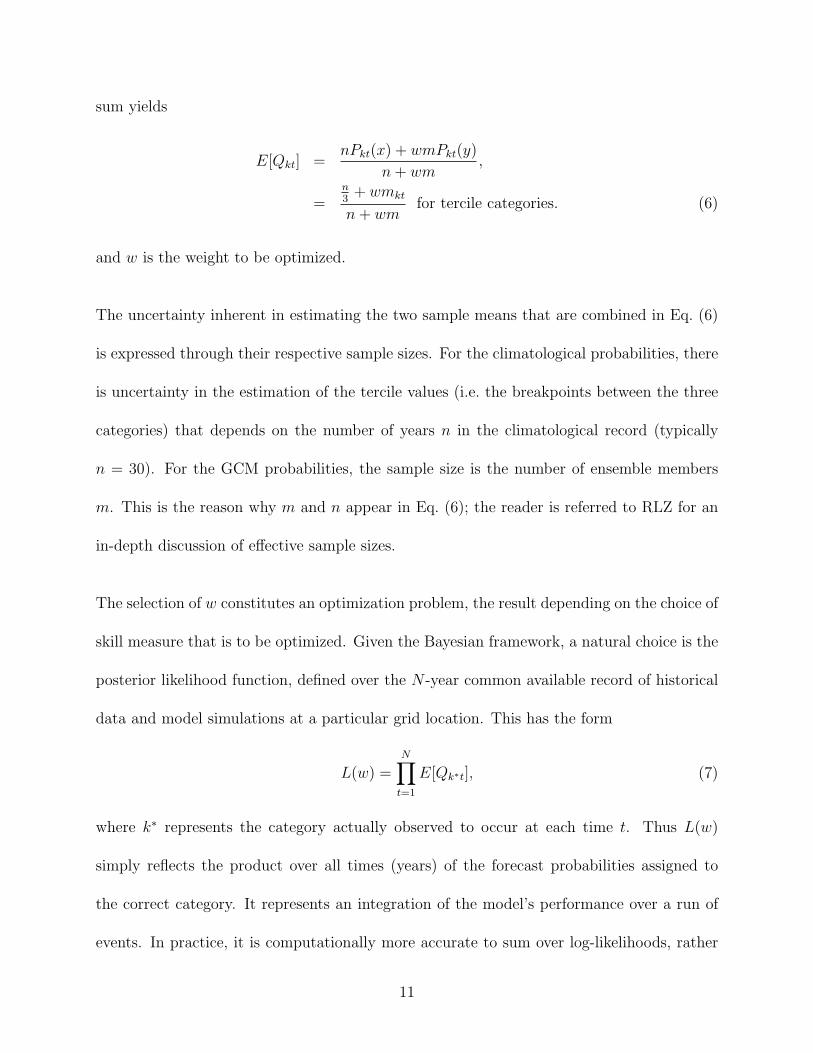
sum yields
E[Qkt] =nPkt(x) + wmPkt(y)
n + wm,
=n3
+ wmkt
n + wmfor tercile categories. (6)
and w is the weight to be optimized.
The uncertainty inherent in estimating the two sample means that are combined in Eq. (6)
is expressed through their respective sample sizes. For the climatological probabilities, there
is uncertainty in the estimation of the tercile values (i.e. the breakpoints between the three
categories) that depends on the number of years n in the climatological record (typically
n = 30). For the GCM probabilities, the sample size is the number of ensemble members
m. This is the reason why m and n appear in Eq. (6); the reader is referred to RLZ for an
in-depth discussion of effective sample sizes.
The selection of w constitutes an optimization problem, the result depending on the choice of
skill measure that is to be optimized. Given the Bayesian framework, a natural choice is the
posterior likelihood function, defined over the N -year common available record of historical
data and model simulations at a particular grid location. This has the form
L(w) =N∏
t=1
E[Qk∗t], (7)
where k∗ represents the category actually observed to occur at each time t. Thus L(w)
simply reflects the product over all times (years) of the forecast probabilities assigned to
the correct category. It represents an integration of the model’s performance over a run of
events. In practice, it is computationally more accurate to sum over log-likelihoods, rather
11

than computing the product of likelihoods over all times. Similar results are obtained by
minimizing the sum of squared errors, or by maximizing the RPSS.
3.2 Combining several models
The above scheme was generalized by RLZ to construct a posterior probability forecast
through a combination of forecasts from J different models plus a climatological forecast.
The mean of the posterior categorical probability forecast is then defined as
E[Qkt] =
∑J+1j=1 wjmjPjkt(y)∑J+1
j=1 wjmj
, (8)
where mj is the size of the ensemble for model j (mj = n for climatology) and wj is the
weight given to model j. The weights are determined by maximizing the posterior likelihood
function as before [Eq. (7)].
This scheme has been used successfully at the International Research Institute for Climate
Prediction (IRI) to make routine seasonal climate forecasts using 3–6 GCMs (Barnston et al.
2003). However, estimation difficulties started to arise when more models became available
and were added to the mix, at the same time as the common training period available became
restricted to only N = 33 years. The resulting weight maps became more noisy and speckled
in appearance (cf. RLZ). Upon closer inspection, it was found (not shown) that the weights
often become exactly zero for all except one model (or climatology), so that the scheme [Eq.
(8)] tends to “choose” one (or two) particulars model(s), with large variability in this choice
between neighboring model gridboxes. This problem appears to be associated with the high
dimension of the optimization space, given the short length of the time series: the likelihood
12

in (7) has to be maximized over a J-dimensional space of model weights, using only N years
of data.
To circumvent the problem of the increasingly high dimensionality of the optimization space
with increasing J , we now introduce a two-stage optimization procedure, wherein the model
combination is always limited to a single model plus climatology, as given by Eq. (6).
In stage one, each model is combined with the climatological forecast individually by per-
forming J separate optimizations using (6) and (7). This yields a set of model weights w(1)j
(j = 1 . . . J) that express each model’s performance compared to an n-yr climatology.
In stage two, we combine the forecast-probabilities of the J models together according to
these weights w(1)j to form a new set of GCM forecast probabilities
P(2)kt (y) =
1∑j w
(1)j
J∑j=1
w(1)j
mjkt
mj
. (9)
Eq. (6) is then solved for w(2), by substituting P(2)kt (y) and m(2) =
∑Jj=1 mj, and then using
Eq. (7) as before. The final weights of the individual models are then disaggregated according
to their values in stage one:
w′j =
1∑j w
(1)j
w(1)j w(2). (10)
The weight-maps (not shown) produced using Eqs. (9, 10) are much more evenly weighted
between models, than those from Eq. (8), but they continue to exhibit noise at the gridbox
scale. The short length of the training dataset used to derive the weights (48 years) suggests
that sampling variability is still potentially a problem. To help alleviate this, a “cross-
validation” was performed, repeating the entire two-stage procedure 43 times. Each time, a
contiguous block of 6 years was withheld from the dataset, and the optimal weights computed.
13

The resulting 43 estimates of the optimal weights were then simply averaged together. This
“cross validation” is designed to reduce the effects of sampling variations on the optimization;
it has the effect of largely removing the white areas on the weight maps where weights are
zero, replacing them with small values (< 0.1) (not shown). The observed and model tercile-
values were kept fixed at their 1968–97 values. Little sensitivity was found to recomputing
them from the 42-yr sub-sample each time.
Up until this point, we have computed the weights independently at each of the 2829 land
gridboxes of the models. While the resolution of a GCM is nominally at the gridbox scale, it
is not expected to be as skillful at this scale as at more aggregated scales (Gong et al. 2003),
and much of the variability in model weights between adjacent gridboxes must be regarded
as sampling variability. To this end, we introduce a 9-point binomial spatial smoother into
the two-stage cross-validated algorithm. In this case we maximize the likelihood:
L(w) =9∏
i=1
n∏t=1
E[Qitk∗ ], (11)
where the i subscript sums over adjacent gridpoints. The central point is counted twice (to
give a binomial smoother) and gridboxes that fall over ocean areas are excluded (for which
there is no observational verification data).
The weights assigned to the climatological equal-odds forecast are plotted in Fig. 1, computed
using the revised two-stage scheme, including cross-validation and spatial averaging of the
likelihood function. Here we plot the normalized climatological weights wClim = n/(n +
m(2)w(2)), so that the climatological and model weights sum to 1 at each gridbox. The optimal
climatological weights are smaller for temperature than for precipitation, consistent with
14

the higher skill of a thermodynamic quantity (temperature) compared to a dynamical one
(precipitation). The higher skill derives both from the higher physical predictability of land
temperature (given SST), as well as the greater ability of GCMs to represent temperature
compared to precipitation. The wClim exhibits considerable spatial and seasonal variation.
The red shading (wClim > 0.8) occurs at many locations in the precipitation-weight maps,
denoting areas where the multi-model ensemble hindcasts lack skill; forecasts issued for these
regions will largely resort to the “prior” climatological forecast probabilities, with near-zero
RPSS. It will be seen below in Tables 2 and 3 that this largely removes negative values in
spatial averages of RPSS.
The optimal model weights for JAS precipitation are shown in Fig. 2, with the normalization
wModel = w′m(2)/(n + m(2)w(2)). The weights of the individual models often tend to be in
the range 0.1–0.3, for the six-model combination. In many areas, the revised scheme tends
to weight the models fairly evenly. Nonetheless, closer inspection reveals important inter-
model differences that may be informative to model developers. Figure 3 shows the optimal
model weights for JAS temperature which are, not surprisingly, generally somewhat larger
than for precipitation. The 24-member ECHAM4.5 model receives higher weights in both
precipitation and temperature than the other 5 models which have only 9–10 members (Table
1). The effect of ECHAM4.5 ensemble size is investigated in Sect. 4. In general, the weight
maps in Figs. 1–3 are less noisy than those of RLZ, and better reflect the spatial scale on
which GCMs are expected to be more skillful.
15

4 Combined model skill
4.1 Time average RPSS maps
Figure 4 shows maps of time-average RPSS for precipitation and temperature during JAS,
for both the simple pooled multi-model ensemble and the optimal combination, together with
the difference between them. In all cases the RPSS is cross-validated as described in Sect.
2, so that the weights and RPSS are not computed from the same data. The models’ skill
varies considerably by geographical location and by variable. Indeed, the JAS precipitation
skill is highly regional, and is confined to most of South America, equatorial Africa, South
Asia and Australasia; this skill originates from the sensitivity of the tropical atmosphere to
SST anomalies and to the El Nino-Southern Oscillation (ENSO) phenomenon in particular
(Ropelewski and Halpert 1987, Barnston and Smith 1996). The precipitation skill of the
simple pooled ensemble is largely negative in the extratropics.
The optimal multi-model combination replaces much of the extensive extratropical areas of
negative precipitation RPSS, with near-zero values. From Fig. 1, this can be seen to be
due to the high weighting given to the climatological forecast in many of these areas, clearly
demonstrating the impact of including the climatology in the multi-model combination. The
impact is smaller in the more-skillful temperature hindcasts, although the negative RPSS
values over Amazonian and Indonesian are much reduced in the optimal combination. The
difference maps (Figs. 4e and 4f) demonstrate that the optimal combination is generally
considerably more skillful than the simple pooling for both precipitation and temperature.
16

There are, nonetheless a few regions of decreasing skill, particularly in temperature over
North America and Siberia.
4.2 RPSS of individual models
The RPSS of the individual models and various multi-model ensembles are summarized in
Tables 2 and 3, in terms of spatio-temporal averages over the land areas of the tropics and
extratropics (divided at 30o latitude). For precipitation (Table 2), all the individual models
have negative skills (i.e. worse than climatology) in both domains. This is largely the case
for temperature as well, except when all 24 members are included in the ECHAM4 ensemble
(Table 3). Increasing the ensemble size here has a clear benefit on both temperature and
precipitation RPSS averages. The pooled ensembles perform much better than the individual
models, but the average RPSS are still near-zero for precipitation over these large domains.
4.3 Combinations of 3 vs. 6 models
The sensitivity of the RPSS to the number of models included in the ensemble is shown
in Tables 2 and 3 and Figs. 5 and 6, for both the pooled ensemble and optimal model
combination. Here we compare the full 6 models, against all possible (i.e. 20) subsets of 3
models. To construct Figs. 5 and 6, we firstly identified the best, middle and worst 3-model
subsets by ranking the 20 time-averaged RPSS scores. We then plot the time series of these
three particular 3-model subsets, together with the full 6-model combination. In Tables 2
17
and 3, we simply give the range of RPSS over all 20 possible subsets.
Combining 6 models instead of 3 almost always leads to increases in skill. The payoff is
larger for the simple pool than for the optimal combination. If we know a priori which three
models to pick, the increase in skill of adding the remaining three models is often quite
modest.
The RPSS of the 6-model optimal combination with the extended 24-member ECHAM4 en-
semble is denoted in Tables 2 and 3 as Cmbo-6+. Even in the optimal 6-model combination,
including an additional 14 ECHAM4 members does yield increases in overall skill. However,
the benefit of increasing the number of models is likely to be greater than the mere increase
in the number of ensemble members (Pavan and Doblas-Reyes 2000).
4.4 Interannual skill variations
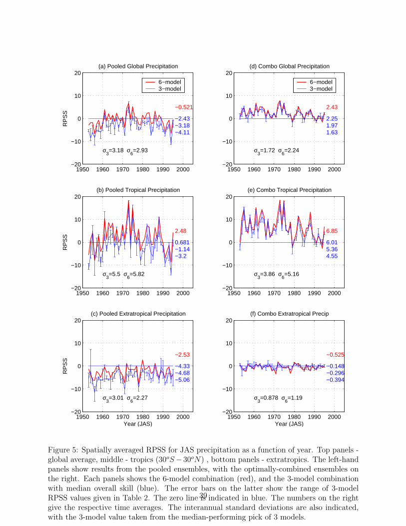
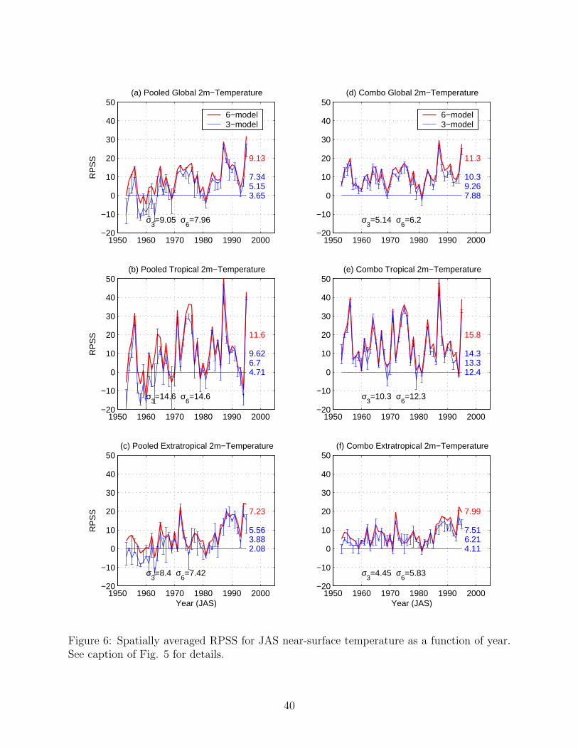
Timeseries of spatially-averaged RPSS are plotted in Figs. 5 and 6. In general, interannual
variations in skill are larger in the tropics than the extratropics for both precipitation and
temperature. This reflects the fact that interannual anomalies in tropical SST such as El
Nino produce large responses in the tropics, but much less so in the extratropical spatial
average. The peaks in skill are consistent with the timing of ENSO events (Goddard, in
preparation). Note that the spatial averages are not weighted by area and are thus biased
toward higher latitudes, due to the convergences of the meridians.
Figure 5 clearly illustrates how the optimal weighting boosts the tropical skill of precipi-
18

tation forecasts in years in which it is relatively low, reducing the amount of interannual
and interdecadal skill variability. In the extratropics, substantial spurious interannual vari-
ation in the pooled-model skill are largely eliminated in the optimal combination, to yield
near-zero RPSS in all years. Similar comments apply to temperature (Fig. 6), although
interannual variations in skill are larger. In the extratropics there appears to be a trend
toward increasing temperature skill; this may be an artefact associated with recent trends
upward in temperature, together with the use of a fixed climatological normal.
4.5 Comparison with the RLZ scheme
The skill of the revised multi-model optimal combination is compared to the original RLZ
scheme in Tables 2 and 3. The revised Bayesian scheme of Eqs. (9–11) is found to be more
skillful on average than the RLZ scheme [Eqs. (7–8)], especially for precipitation. This is
also clear in RPSS maps similar to Fig. 4 (not shown). Tables 2 and 3 also indicate that for 6
models, the RLZ scheme is actually less skillful than the pooled ensemble in the extratropics
for both precipitation and temperature. All our computations with the RLZ scheme were
performed with the “cross validation” described in Sect. 3, so that sampling variability should
be reduced compared to the results reported by RLZ.
19

5 Discussion and conclusions
An improved Bayesian weighting scheme is developed and used to combine several atmo-
spheric GCM ensemble categorical seasonal predictions of precipitation or near-surface tem-
perature over land, based on the prior belief that the GCM forecast probabilities are equal
to climatological probabilities of 1/3. The scheme’s skill is compared against the individual
model-ensembles (with 9–24 members), simple pooled ensembles of three and six models,
as well as the original version of the Bayesian weighting scheme devised by Rajagopalan,
Lall and Zebiak (2002) (RLZ). The Ranked Probability Skill Score (RPSS) is used as the
skill measure, cross-validated by withholding six contiguous years at a time from the 48-yr
1950–97 timeseries of model simulations and observed precipitation and temperature.
Our results demonstrate clear gains in skill by simply pooling together the ensemble hindcasts
made with individual GCM ensembles, corroborating previous studies (Fraedrich and Smith
1989; Graham et al. 2000; Palmer et al. 2000; Pavan and Doblas-Reyes 2000; Peng et al.
2002). A pooling of six models is found to be almost always superior to a pooling of just
three models, although the gain is modest if the three best models (measured over the 46-yr
period used to compute RPSS) can be identified a priori. As expected, the precipitation
skill is higher within the tropics than in the extratropics, and the temperature skill is higher
than for precipitation.
The revised Bayesian optimal weighting scheme is shown to outperform the pooled ensemble.
In the extratropics, its main impact is to bring much of the large area of negative precipi-
tation RPSS up to near-zero values. Effectively, it progressively replaces the model forecast
20

with climatological equal-odds values in these areas by downweighting the model forecasts
relative to the climatological one. There are also substantial gains in the average tropical
precipitation skill. Increases in skill are more modest for the temperature hindcasts, which
are more skillful to begin with. However, there are nonetheless regions of negative RPSS in
the pooled ensemble that are much reduced in the optimal combination. Interannual vari-
ations in skill are reduced, especially in extratropical precipitation, where they are largely
spurious.
Improvements made to the original Bayesian scheme in the form of reducing the dimen-
sionality of the numerical optimization and including spatial smoothing of the likelihood
function are shown to substantially increase the RPSS cross-validated skills. Maps of the
model weights are less noisy than in the original scheme, and the weights are distributed
more evenly among the models.
The number of parameters to be estimated increases with the number of models, leading to
a decrease in the degrees of freedom available for estimating the likelihood function in the
weight-optimization. This translates into higher variability in the optimal weights selected
and hence a degradation in the performance of the “best” model selected. In the revised
scheme, each model is first calibrated against climatology independently, and this potentially
leads to a more robust weighting and smoothing of that model’s results towards climatology.
Since the smoothed models have lower variance, the results from their subsequent combina-
tion may still be improved over the RLZ scheme. Even though the degrees of freedom are
still reduced by adding additional models (because the number of parameters to be estimated
increases), each model brought into the mix has potentially lower variability. The spatial
21

averaging used in the revised scheme further reduces this variability in model selection.
Multiple co-linearity is often a concern when combining together several predictors using
multiple linear regression. In the context of the multi-model ensemble, consider the case of
two identical GCMs run with the same number of ensemble members, but from a different set
of initial conditions. In the one-stage scheme of RLZ [Eq. (8)], there will be non-uniqueness
in the weights assigned to the two models, since any combination of them will yield a similar
log-likelihood score. However, a forecast made with the multi-model ensemble will not be
impacted, and this only presents a problem if we wish to use the “optimal” weights to at-
tribute skill to either model. In contrast, the revised two-stage scheme does not suffer from
this non-uniqueness in the weights. Each model is calibrated independently against clima-
tology, so two near-identical GCMs will receive similar weight, whose magnitude depends
upon skill against climatology; any co-linearity of errors will not be reflected in the weights.
Maps of the optimal model weights, such as Figs. 2 and 3, provide a useful byproduct of
the optimal weighting exercise. The maps provide an additional metric of model skill and
intercomparison that may be of value to GCM developers.
One weakness of the Bayesian scheme that persists despite the improvements to the algorithm
is an occasional tendency toward high GCM precipitation weights in some high latitude
regions (see Fig. 4). We would not expect the GCMs’ precipitation hindcasts to be skillful
in many of these regions. If the GCM probabilities—or the combined second-stage model
probabilities in Eq. (9)—beat the climatological ones over the training period, even by a slight
amount, then the optimal combination can heavily favor the model. In effect, the likelihood-
22

optimization is not sensitive to distance. The cross-validation and spatial averaging do
alleviate the problem to some extent because they reduce sampling variability, which is the
root of the spurious model skill in question. No account was taken of the convergence of the
meridians toward to the poles. In future work, the spatial smoothing could be performed
over a fixed area, rather than a fixed number of gridpoints. However, sampling variability
will never be completely eliminated given the relatively short records available.
The revised scheme appears to be well suited to combining larger sets of models and, in the
future, it should be possible to include statistical models into the weighted ensemble without
fundamental difficulty. The skill of the optimal combination is always increased (at least in
the large spatial averages considered) when the number of models in the combination is
increased from 3 to 6, regardless of which models are included in the 3-model combination.
With the exception of the 24-member ECHAM4 ensemble, the number of ensemble members
for each model was limited to about 10. Increasing the size of the ECHAM4 model ensemble
from 10 to 24 members increases this individual model’s RPSS substantially and even has
a positive impact on the six-model combination. Thus, there is a potential payoff to be
achieved by increasing the size of the model ensembles.
Finally, it should be remembered that the RPSS skills reported in this paper apply to the
case of prescribed monthly-mean SST. These skills decrease substantially in retrospective
forecasts in which predicted SST is used to force the atmospheric GCMs. On the other hand,
some increased skill can be expected from initializing the models with observed estimates of
soil moisture and snow cover. In any case, optimally-weighted multi-model ensembles form
a valuable component of a seasonal climate forecasting system.
23

Acknowledgements: We are grateful to Tony Barnston, Simon Mason and Balaji Rajagopalan
for helpful discussions, and Tony Barnston for his valuable comments on an earlier version
of the manuscript. We especially wish to thank the six GCM modeling centers whose model
runs formed the basis for our study. This work was supported by the International Research
Institute for Climate Prediction and a National Oceanic and Atmospheric Administration
Grant.
24

6 References
Barnston, A. G., and T. M. Smith, 1996: Specification and Prediction of Global
Surface Temperature and Precipitation from Global SST Using CCA. J.
Climate, 9, 2660-2697.
Barnston, A. G., S. J. Mason, L. Goddard, D. G. DeWitt, and S. E. Zebiak, 2003:
Multi-model ensembling in seasonal climate forecasting at IRI. Bull. Amer.
Meteor. Soc., in press.
Doblas-Reyes, F. J., M. Deque, and J.-P. Piedelievre, 2000: Multi-model spread
and probabilistic seasonal forecasts in PROVOST. Quart. J. Royal Meteor.
Soc., 126, 2069-2088.
Epstein, E. S., 1969: A scoring system for probability forecasts of ranked cate-
gories. J. Appl. Meteor., 8, 985-987.
Fraedrich, K., and N. R. Smith, 1989, Combining predictive schemes in long
range forecasting, J. Climate, 2, 291-294.
Gelman, A., J. B. Carlin, H. S. Stern, and D. B. Rubin, 1995: Bayesian Data
Analysis, Chapman and Hall, 526pp.
Goddard, L., 2003: El Nino: Catastrophe or opportunity?. Submitted to Nature.
Goddard, L., A. G. Barnston, and S. J. Mason, 2003: Evaluation of the IRI’s
“net assessment” seasonal climate forecasts: 1997–2001. Bull. Amer. Met.
Soc., in press.
Graham, R. J., A. D. L. Evans, K. R. Mylne, M. S. J. Harrison, and K. B.
25

Robertson, 2000: An assessment of seasonal predictability using atmospheric
general circulation models. Quart. J. Royal Meteor. Soc., 126, 2211-2240.
Gong, X., A. G. Barnston, and M. N. Ward, 2003: The Effect of Spatial Ag-
gregation on the Skill of Seasonal Precipitation Forecasts. J. Climate, 16,
3059-3071.
Hack, J. J., J. T. Kiehl, and J. W. Hurrell, 1998: The hydrological and thermo-
dynamic characteristics of the NCAR CCM3. J. Climate, 11,, 1179-1206.
Hagedorn, R., 2001: Development of a multi-model ensemble system for seasonal
to interannual prediction. XXVI General Assembly of the EGS, Nice, France,
March 2001.
Kanamitsu, M., and Coauthors, 2002: NCEP Dynamical Seasonal Forecast Sys-
tem 2000, Bull. Amer. Met. Soc., 83, 1019-1037.
Kanamitsu, M., and K. C. Mo, 2003: Dynamical Effect of Land Surface Processes
on Summer Precipitation over the Southwestern United States, J. Climate,
16, 496-509.
Kumar, A., M. P. Hoerling, M. Ji, A. Leetmaa, and P. Sardeshmukh, 1996:
Assessing a GCM’s suitability for making seasonal predictions. J. Climate,
9, 115-129.
Kumar, A., A. G. Barnston, and M. P. Hoerling, 2001: Seasonal predictions,
probabilistic verifications, and ensemble size. J. Climate, 14, 1671-1676.
Lorenz, E. N., 1963: Deterministic Nonperiodic Flow. J. Atmos. Sci., 20, 130-
26

148.
New, M., M. Hulme, and P. D. Jones, 1999: Representing twentieth-century
space-time climate variability. Part I: Development of a 1961-90 mean monthly
terrestrial climatology. J. Climate, 12, 829-856.
New, M., M. Hulme, and P. D. Jones, 2000: Representing twentieth-century
space-time climate variability. Part I: Development of a 1961-90 monthly
grid of terrestrial surface climate. J. Climate, 13, 2217-2238.
Palmer, T. N., C. Brankovic, D. S. Richardson, 2000: A probability and decision-
model analysis of PROVOST seasonal multi-model ensemble integrations.
Quart. J. Royal Meteor. Soc., 126, 2013-2034.
Pavan, V., and F. J. Doblas-Reyes, 2000: Multi-model seasonal hindcasts over the
Euro-Atlantic: skill scores and dynamic features, Climate Dyn., 16, 611-625.
Peng et al. 2002
Rajagopalan, B., U. Lall, and S. E. Zebiak, 2002: Categorical climate forecasts
through regularization and optimal combination of multiple GCM ensembles.
Mon. Weather Rev., 130, 1792-1811.
Reynolds, R. W., 1988: A Real-Time Global Sea Surface Temperature Analysis.
J. Climate, 1, 7587.
Reynolds, R. W., and T. M. Smith, 1994: Improved Global Sea Surface Temper-
ature Analyses Using Optimum Interpolation. J. Climate, 7, 929948.
Roeckner, E., and Coauthors, 1996: The atmospheric geneal circulation model
27
ECHAM4: Model description and simulation of present-day climate. Max-
Planck-Institut fur Meteorologie Rept. 218, 90pp.
Ropelewski, C. F., and M. S. Halpert, 1987: Global and Regional Scale Pre-
cipitation Patterns Associated with the El Nio/Southern Oscillation. Mon.
Weather Rev., 115, 1606-1626.
Wilks, D.S., 1995: Statistical Methods in the Atmospheric Sciences. Interna-
tional Geophysical Series, 59, Academic Press, 464 pp.
28

List of Tables
1 The six GCMs used in the combinations. . . . . . . . . . . . . . . . . . . . . 32
2 Spatially averaged RPSS for precipitation, over the tropics (30oS − 30oN)
and extratropics (poleward of 30o), for the individual models and various
multi-model ensembles. Key: Pool–pooled ensemble, Cmbo–revised two-stage
Bayesian combination with spatial smoothing of objective function, RLZ–
Bayesian combination of Rajagopalan et al. (2002) (with cross-validation).
The -n suffix denotes the number of models in the ensemble. The 3-model
combination is given as the range of all 20 possible such combinations. The
ECHAM4+, Cmbo-6+ and RLZ-6+ entries use the extended 24-member en-
semble; all other entries use a 10-member ECHAM4 ensemble. All results are
for the 1953–95 period. . . . . . . . . . . . . . . . . . . . . . . . . . . . . . . 33
3 Spatially averaged RPSS for near-surface temperature. See Table 2 for details. 34
29

List of Figures
1 The weight values assigned to the climatological forecast by the revised 6-
model optimal combination scheme. (a) JFM precipitation, (b) JFM temper-
ature, (c) JAS precipitation, (b) JAS temperature. Weights < 0.01 are shaded
white. . . . . . . . . . . . . . . . . . . . . . . . . . . . . . . . . . . . . . . . 35
2 The weight values assigned to each model forecast by the revised 6-model op-
timal combination scheme, for JAS precipitation. Weights < 0.01 are shaded
white. . . . . . . . . . . . . . . . . . . . . . . . . . . . . . . . . . . . . . . . 36
3 The optimal model weights from the revised 6-model combination for JAS
near-surface temperature. Weights < 0.01 are shaded white. . . . . . . . . . 37
4 The RPSS of 6-model ensembles of JAS precipitation (left) and JAS near-
surface temperature (right). (a) and (b): simple pooled ensembles; (c) and
(d): optimal combinations; (e) and (f): differences between pooled and op-
timal combinations. Blue denotes negative RPSS, near-zero values (i.e. the
climatological forecast) are white, and positive RPSS are denoted by yellow
and red. The pooled ensemble comprises all six models with 83 members in
total. All values computed for 1953–95. Absolute RPSS differences < 2% are
shaded white in (e) and (f). . . . . . . . . . . . . . . . . . . . . . . . . . . . 38
30

5 Spatially averaged RPSS for JAS precipitation as a function of year. Top
panels - global average, middle - tropics (30oS − 30oN) , bottom panels -
extratropics. The left-hand panels show results from the pooled ensembles,
with the optimally-combined ensembles on the right. Each panels shows the
6-model combination (red), and the 3-model combination with median overall
skill (blue). The error bars on the latter show the range of 3-model RPSS
values given in Table 2. The zero line is indicated in blue. The numbers on the
right give the respective time averages. The interannual standard deviations
are also indicated, with the 3-model value taken from the median-performing
pick of 3 models. . . . . . . . . . . . . . . . . . . . . . . . . . . . . . . . . . 39
6 Spatially averaged RPSS for JAS near-surface temperature as a function of
year. See caption of Fig. 5 for details. . . . . . . . . . . . . . . . . . . . . . . 40
31

Table 1: The six GCMs used in the combinations.
Model ECHAM4.5 NCEP-MRF9 NSIPP1 COLA CCM3.2 ECPC
Ensemble size 24 10 9 10 10 10
Horizontal resolution T42 T40 2.5o T63 T42 T62
Number of levels 19 18 34 18 18 28
ECHAM: Max Planck Institute for Meteorology, Hamburg, Germany (Roeckner et al. 1996),
http://www.mpimet.mpg.de/en/extra/models/echam/index.php.
NCEP-MRF: National Centers for Environmental Prediction - Medium Range Forecast model
(Kumar et al. 1996).
NSIP: NASA’s Seasonal to Interannual Prediction Project at Goddard Space Flight Center,
http://nsipp.gsfc.nasa.gov/atmos/atmosdescrip.html.
COLA: Center for Ocean-Land-Atmosphere studies,
http://www-pcmdi.llnl.gov/modeldoc/amip1/14cola ToC.html.
CCM: National Centers for Atmospheric Research (NCAR) Community Climate Model
(Hack et al. 1998), http://www.cgd.ucar.edu/cms/ccm3.
ECPC: Experimental Climate Prediction Center at Scripps Institution of Oceanography;
a revised version of the GCM earlier implemented at NOAA/NCEP (Kanamitsu et al. 2002),
with some changes to the physics as described in Kanamitsu and Mo (2003).
32

Table 2: Spatially averaged RPSS for precipitation, over the tropics (30oS−30oN) and extra-
tropics (poleward of 30o), for the individual models and various multi-model ensembles. Key:
Pool–pooled ensemble, Cmbo–revised two-stage Bayesian combination with spatial smooth-
ing of objective function, RLZ–Bayesian combination of Rajagopalan et al. (2002) (with
cross-validation). The -n suffix denotes the number of models in the ensemble. The 3-model
combination is given as the range of all 20 possible such combinations. The ECHAM4+,
Cmbo-6+ and RLZ-6+ entries use the extended 24-member ensemble; all other entries use
a 10-member ECHAM4 ensemble. All results are for the 1953–95 period.
Jan–Mar (JFM) Jul–Sep (JAS)
Tropics Extratropics Tropics Extratropics
ECHAM4 −12.35 −9.41 −7.71 −11.33
ECHAM4+ −8.04 −4.04 −3.22 −5.85
NCEP −18.72 −11.27 −14.30 −12.81
NSIPP1 −20.40 −11.75 −19.76 −13.83
COLA −22.83 −13.68 −23.59 −13.67
CCM3 −13.54 −8.69 −15.54 −12.81
ECPC −14.07 −14.79 −15.10 −13.76
Pool-3 −5.82 – −1.87 −4.16 – −1.90 −3.20 – 0.68 −5.06 – −4.33
Pool-6 −0.35 −0.24 3.08 −2.21
Cmbo-3 2.33 – 3.10 −0.06 – 0.24 4.55 – 6.01 −0.39 – −0.15
Cmbo-6 3.30 0.19 6.85 −0.53
Cmbo-6+ 3.39 0.44 6.97 −0.55
RLZ-6+ 1.42 −1.12 5.26 −2.3733

Table 3: Spatially averaged RPSS for near-surface temperature. See Table 2 for details.
Jan–Mar (JFM) Jul–Sep (JAS)
Tropics Extratropics Tropics Extratropics
ECHAM4 −1.03 −4.82 −1.35 −4.36
ECHAM4+ 2.76 −0.14 2.24 1.01
NCEP −7.99 −14.40 −16.35 −11.05
NSIPP1 −7.28 −11.36 −15.23 −11.66
COLA −19.62 −17.90 −19.84 −12.59
CCM3 1.18 −4.21 −4.60 −5.15
ECPC −2.00 −6.63 −10.41 −7.81
Pool-3 8.40 – 11.22 −0.68 – 4.17 4.71 – 9.62 2.0 – 5.56
Pool-6 13.41 4.95 11.79 7.38
Cmbo-3 12.50 – 14.71 2.69 – 4.49 12.44 – 14.31 4.11 – 7.51
Cmbo-6 15.68 5.07 15.78 7.99
Cmbo-6+ 15.75 5.27 16.01 8.16
RLZ-6+ 14.79 4.01 15.48 7.35
34

Figure 1: The weight values assigned to the climatological forecast by the revised 6-modeloptimal combination scheme. (a) JFM precipitation, (b) JFM temperature, (c) JAS precip-itation, (b) JAS temperature. Weights < 0.01 are shaded white.35

Figure 2: The weight values assigned to each model forecast by the revised 6-model optimalcombination scheme, for JAS precipitation. Weights < 0.01 are shaded white.
36

Figure 3: The optimal model weights from the revised 6-model combination for JAS near-surface temperature. Weights < 0.01 are shaded white.
37

Figure 4: The RPSS of 6-model ensembles of JAS precipitation (left) and JAS near-surfacetemperature (right). (a) and (b): simple pooled ensembles; (c) and (d): optimal combi-nations; (e) and (f): differences between pooled and optimal combinations. Blue denotesnegative RPSS, near-zero values (i.e. the climatological forecast) are white, and positiveRPSS are denoted by yellow and red. The pooled ensemble comprises all six models with 83members in total. All values computed for 1953–95. Absolute RPSS differences < 2% areshaded white in (e) and (f).
38
1950 1960 1970 1980 1990 2000−20
−10
0
10
20(a) Pooled Global Precipitation
RP
SS
σ3=3.18 σ
6=2.93
−0.521
−2.43−3.18−4.11
6−model3−model
1950 1960 1970 1980 1990 2000−20
−10
0
10
20(b) Pooled Tropical Precipitation
RP
SS
σ3=5.5 σ
6=5.82
2.48
0.681−1.14−3.2
1950 1960 1970 1980 1990 2000−20
−10
0
10
20(c) Pooled Extratropical Precipitation
RP
SS
Year (JAS)
σ3=3.01 σ
6=2.27
−2.53
−4.33−4.68−5.06
1950 1960 1970 1980 1990 2000−20
−10
0
10
20(d) Combo Global Precipitation
σ3=1.72 σ
6=2.24
2.43
2.251.971.63
6−model3−model
1950 1960 1970 1980 1990 2000−20
−10
0
10
20(e) Combo Tropical Precipitation
σ3=3.86 σ
6=5.16
6.85
6.015.364.55
RPSS of JAS ppt
1950 1960 1970 1980 1990 2000−20
−10
0
10
20(f) Combo Extratropical Precip
Year (JAS)
σ3=0.878 σ
6=1.19
−0.525
−0.148−0.296−0.394
Figure 5: Spatially averaged RPSS for JAS precipitation as a function of year. Top panels -global average, middle - tropics (30oS− 30oN) , bottom panels - extratropics. The left-handpanels show results from the pooled ensembles, with the optimally-combined ensembles onthe right. Each panels shows the 6-model combination (red), and the 3-model combinationwith median overall skill (blue). The error bars on the latter show the range of 3-modelRPSS values given in Table 2. The zero line is indicated in blue. The numbers on the rightgive the respective time averages. The interannual standard deviations are also indicated,with the 3-model value taken from the median-performing pick of 3 models.
39
1950 1960 1970 1980 1990 2000−20
−10
0
10
20
30
40
50(a) Pooled Global 2m−Temperature
RP
SS
σ3=9.05 σ
6=7.96
9.13
7.345.153.65
6−model3−model
1950 1960 1970 1980 1990 2000−20
−10
0
10
20
30
40
50(b) Pooled Tropical 2m−Temperature
RP
SS
σ3=14.6 σ
6=14.6
11.6
9.626.74.71
1950 1960 1970 1980 1990 2000−20
−10
0
10
20
30
40
50(c) Pooled Extratropical 2m−Temperature
RP
SS
Year (JAS)
σ3=8.4 σ
6=7.42
7.23
5.563.882.08
1950 1960 1970 1980 1990 2000−20
−10
0
10
20
30
40
50(d) Combo Global 2m−Temperature
σ3=5.14 σ
6=6.2
11.3
10.39.267.88
6−model3−model
1950 1960 1970 1980 1990 2000−20
−10
0
10
20
30
40
50(e) Combo Tropical 2m−Temperature
σ3=10.3 σ
6=12.3
15.8
14.313.312.4
RPSS of JAS 2mT
1950 1960 1970 1980 1990 2000−20
−10
0
10
20
30
40
50(f) Combo Extratropical 2m−Temperature
Year (JAS)
σ3=4.45 σ
6=5.83
7.99
7.516.214.11
Figure 6: Spatially averaged RPSS for JAS near-surface temperature as a function of year.See caption of Fig. 5 for details.
40


