

The VLDB Journal manuscript No.(will be inserted by the editor)
Apostol (Paul) Natsev · John R. Smith · Jeffrey S. Vitter
Optimal Incremental Algorithms for Top-k Joins
with User-Defined Join Constraints
Abstract We investigate the problem of incremental joins of multiple ranked data streams when the join
condition is a list of arbitrary user-defined predicates on the input tuples. We propose an algorithm J∗ for
ranked input joins over user-defined join predicates. The basic version of the algorithm uses only sequential
access into the database and is easily pipelinable—that is, the output of one join query can be fed as the
input of another. We also propose a J∗PA algorithm that can exploit available database indexes for efficient
random access based on the join predicates, as well as give ε-approximation versions for both of the above
algorithms. Finally, we prove strong optimality results for J∗ and its approximated version, and we study their
performance empirically.
Keywords Query optimization · Fusion optimization · Rank join · Rank aggregation · J-star algorithms
A. Natsev (contact author)
IBM Thomas J. Watson Research Center
19 Skyline Drive, Hawthorne, NY 10532
Tel.: +1-914-784-7541, Fax: +1-914-784-7455
E-mail: [email protected]
J. R. Smith
IBM Thomas J. Watson Research Center
19 Skyline Drive, Hawthorne, NY 10532
J. S. Vitter
Dean of the College of Science, Purdue University,
150 North University Street, West Lafayette, IN 47907-2067
2 Apostol (Paul) Natsev et al.
1 Introduction
Advances in computing power over the last few years have made a considerable amount of multimedia data
available on the web and in domain-specific applications. The result has been an increasing emphasis on the
requirements for searching large repositories of multimedia data. An important characteristic of multimedia
queries is the fact that they return ordered data as their results, as opposed to returning an unordered set of
answers, as in traditional databases. The results in multimedia queries are usually ranked by a similarity score
reflecting how much each tuple satisfies the query. In addition, users are typically interested only in the top k
answers, where k is very small compared to the total number of tuples. Work in this area has therefore focused
primarily on supporting top-k queries ranked on similarity of domain-specific features, such as color, shape,
etc.
One aspect that has received less attention, however, is the requirement to efficiently combine ranked
results from multiple atomic queries into a single ranked stream. Most systems support some form of search
based on a limited combination of atomic features but the combinations are usually fixed, limited to the types
of features supported internally by the system, and typically allowing only Boolean or weighted averaging
combinations. Most related work has also focused on rank aggregation methods that optimize retrieval or
classification performance as opposed to execution time or database access cost. In general, there has been
relatively little work on optimizing the cost of aggregate top-k queries over arbitrary combinations of multiple
ordered data sets.
This paper formalizes the problem and generalizes it to user-defined join predicates. It also introduces
a fast incremental J∗ algorithm for that problem. The ability to support user-defined join predicates makes
the algorithm suitable for join scenarios that were previously unsupported. In case there are available indexes
supporting access based on user-defined predicates, we also give a predicate access version of our algorithm
that can take advantage of such indexes. We also consider approximation algorithms that trade output accuracy
for reduced database access costs and space requirements. Finally, we study the algorithms both theoretically
and empirically.
The rest of the paper is organized as follows. In the remainder of this section, we motivate and formally
define the problem of top-k join queries on ordered data. We also review relevant work and list our specific
contributions. We then give a detailed description of the J∗ algorithm and its iterative deepening variation in

Optimal Top-k Join Algorithms 3
Rock sample 1
Rock sample 2
"on top of"
Find rock structures most similar to the template.
Query template
(a) Example of the ranked join problem.
S1 S2 Sm
Q1 Q2 Qm
Middleware
1
2
N1
(b) Cost model for the ranked join
problem.
Fig. 1 Illustration of the ranked join problem and its formal cost model.
Section 2. We present the J∗PA algorithm in Section 4, and discuss approximation algorithms in Section 5. In
Section 6, we give some optimality results for the proposed algorithms. The behavior of the J∗ algorithm is
evaluated empirically in Section 7, where we validate our theoretical results in practice. We conclude with a
summary of contributions.
1.1 Motivation
A motivating example to demonstrate the problem of joining multiple concepts with user-specified join con-
straints is the match of strata structures across bore holes in oil exploration services. Petroleum companies
selectively drill bore holes in oil rich areas in order to estimate the size of oil reservoir underground. Readings
from instruments measuring physical parameters, such as conductivity, as well as images of rock samples
from the bore hole are indexed by depth, as in the example shown in Figure 1(a). Traditionally, experienced
human interpreters (mostly geologists) will then label the rock samples and try to co-register the labels of one
bore hole with those of many other bores holes in the neighboring area. The matched labels are then fed into
3D modeling software to reconstruct the strata structure underground, which tells the reservoir size.
The process of rock layer labeling and cross-bore co-registration can be significantly sped up by content-
based image retrieval techniques. An interpreter can issue a query to locate similar looking rock layers in all
bore hole images. An example is illustrated in Figure 1(a), where the query template consists of two rock
types, and specifies that one should be close to and above the other.
4 Apostol (Paul) Natsev et al.
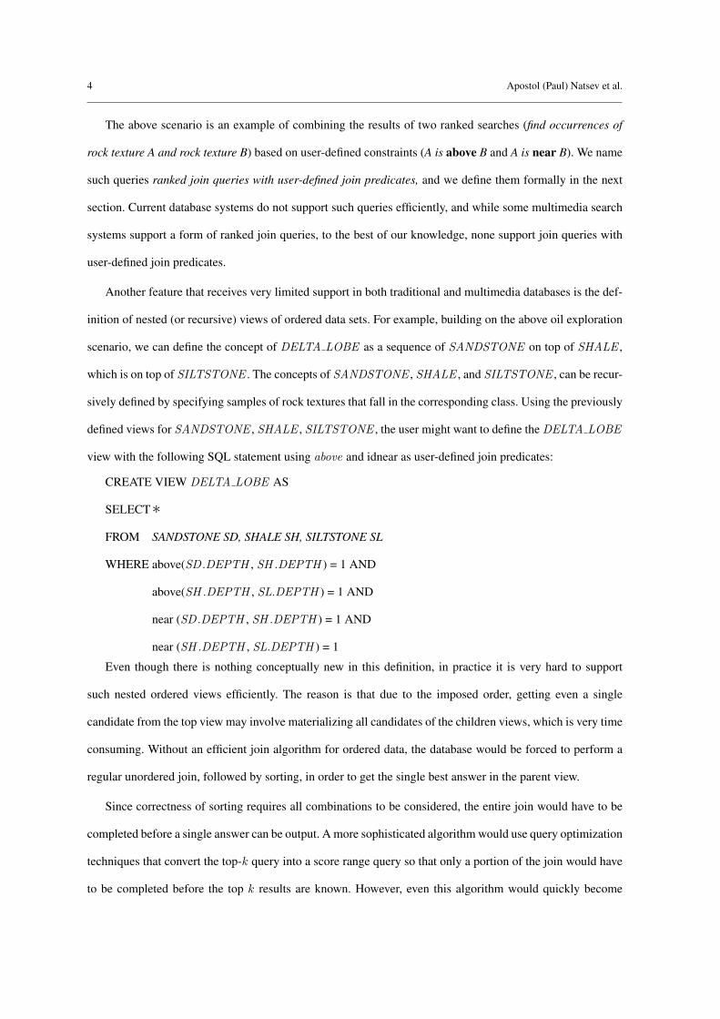
The above scenario is an example of combining the results of two ranked searches (find occurrences of
rock texture A and rock texture B) based on user-defined constraints (A is above B and A is near B). We name
such queries ranked join queries with user-defined join predicates, and we define them formally in the next
section. Current database systems do not support such queries efficiently, and while some multimedia search
systems support a form of ranked join queries, to the best of our knowledge, none support join queries with
user-defined join predicates.
Another feature that receives very limited support in both traditional and multimedia databases is the def-
inition of nested (or recursive) views of ordered data sets. For example, building on the above oil exploration
scenario, we can define the concept of DELTA LOBE as a sequence of SANDSTONE on top of SHALE ,
which is on top of SILTSTONE . The concepts of SANDSTONE , SHALE , and SILTSTONE , can be recur-
sively defined by specifying samples of rock textures that fall in the corresponding class. Using the previously
defined views for SANDSTONE , SHALE , SILTSTONE , the user might want to define the DELTA LOBE
view with the following SQL statement using above and idnear as user-defined join predicates:
CREATE VIEW DELTA LOBE AS
SELECT∗FROM SANDSTONE SD, SHALE SH, SILTSTONE SL
WHERE above(SD .DEPTH , SH .DEPTH ) = 1 AND
above(SH .DEPTH , SL.DEPTH ) = 1 AND
near (SD .DEPTH , SH .DEPTH ) = 1 AND
near (SH .DEPTH , SL.DEPTH ) = 1
Even though there is nothing conceptually new in this definition, in practice it is very hard to support
such nested ordered views efficiently. The reason is that due to the imposed order, getting even a single
candidate from the top view may involve materializing all candidates of the children views, which is very time
consuming. Without an efficient join algorithm for ordered data, the database would be forced to perform a
regular unordered join, followed by sorting, in order to get the single best answer in the parent view.
Since correctness of sorting requires all combinations to be considered, the entire join would have to be
completed before a single answer can be output. A more sophisticated algorithm would use query optimization
techniques that convert the top-k query into a score range query so that only a portion of the join would have
to be completed before the top k results are known. However, even this algorithm would quickly become

Optimal Top-k Join Algorithms 5
inefficient when we consider multiple levels of joins in such views. In that case, a partial join at one level
would require a larger partial join at the lower level. The potion of the views that will need to be scanned
at each level will therefore propagate quickly down the levels and after a few levels, the algorithm would
essentially resort to a full database scan.
In addition to the aforementioned strata matching example, there are numerous other application scenarios
that can benefit greatly from the ability to efficiently join ordered data sets with arbitrary join predicates. This
problem arises in many important applications dealing with ordered inputs and multiple ranked data sets, and
requiring the top k solutions. We use the above oil exploration application as the motivating example and for
illustration purposes, but the problem is also relevant to multimedia databases as well as other application sce-
narios involving optimal resource allocation, scheduling, decision making, tournament or itinerary ranking,
etc. In addition to searching, such technology can be used for filtering, annotation, classification and inferenc-
ing purposes, among others. For example, the decision to buy a house in a certain area may include criteria
about proximity to schools or hospitals, termite populations, as well as demographic factors. Ideally, all of
these constraints should be translated into join predicates and incorporated into a single query. The system
will then perform separate atomic sub-queries, involving both structured and unstructured data, optimize the
execution, and present the overall results in ranked order based on the user-specified criteria.
1.2 Definitions and Problem Formulation
In this section we consider the exact formulation of the top-k join problem. First, we consider the difference
between the top-k selection and top-k join problems. The top-k selection problem involves ranking a collection
of objects based on some scoring function, and selecting the top k objects. The ranking may depend on one
or multiple attributes but all of the information needed to compute the overall score, or rank, of each object
is stored in a single table so no joins are involved. An example, would be a typical content-based retrieval
query: find the top k images most similar to a query image based on some visual feature similarity (e.g.,
color, texture, shape, etc.). The top-k join problem (also known as rank join) is similar to the above but the
information needed to compute the score or rank of each object is spread out among multiple tables, which
need to be joined. An example would be to find the best (house, school) pairs that minimize the total cost of

6 Apostol (Paul) Natsev et al.
housing and school tuition, under the join constraint that the house and school are close to each other (e.g.,
distance(house.location, school .location) ≤ threshold ).
The top-k join problem is illustrated in Figure 1(b). Informally, we are given m streams of objects ordered
on a specific score attribute for each object. We are also given a set of p arbitrary predicates defined on object
attributes from one or more streams. The predicates are illustrated by binary edges in Figure 1(b), even though
they may be of higher degrees. A valid join combination includes exactly one object from each stream subject
to the set of join predicates (an example is denoted with a solid red line in Figure 1(b)). Each combination
is evaluated through a monotone score aggregation function defined on the score attributes of the individual
objects, and we are interested in outputting the k join combinations that have the highest overall scores.
Formally, we define a relational join, or a θ-join to be the combination of two database tables based on a
specified relationship θ between one or more attributes in each table:
A ./θ B = {t = ab | a ∈ A, b ∈ B , θ(a.X, b.Y ) = 1}.
We extend the definition to ranked joins or ordered joins as follows:
Definition 11: [Ranked θ-join] We define a ranked θ-join with respect to aggregation function S as the
combination of two tables ordered on a specific score attribute each and joined according to a specified
relationship θ between one of more attributes in each table. The resulting table is ordered on an aggregate
score attribute computed by the scoring function S :
A ./Sθ B = { t = ab | a ∈ A, b ∈ B , θ(a.X, b.Y ) = 1,
t.score = S (a.score, b.score) },
where A, B , and A ./Sθ B are ordered on their respective score attributes.
Definition 12: [Top-k θ-join problem] Given:
– Tables A = {ai} and B = {bj}, ordered on a score attribute, and of size at most n records each;
– A score aggregation function S : [0, 1]× [0, 1] −→ [0, 1] defined over the score attributes of the join tables
that is monotone and incremental over each of its arguments;
– A set of Boolean predicates θ defined on one or more attributes from A and B .
Output: Top k tuples from A ./Sθ B

Optimal Top-k Join Algorithms 7
The hierarchical (nested) ranked join problem is an instance of the above problem where at least one
of Aor B is the result of another ranked join query. Otherwise, we will refer to the join as a single-level join
problem. An algorithm solving the ranked join problem is incremental if it outputs the results one at a time
in a progressive, non-blocking fashion. An algorithm is pipelinable if it is incremental and can be nested in a
hierarchical fashion (i.e., its outputs can be fed as inputs into a higher level join problem).
The cost model we consider includes the database cost of accessing objects from the individual sorted
streams, or join tables. Assuming that the number of objects in each stream is very large, and the access cost
is the bottleneck, the goal is to minimize the total number of accessed objects needed to materialize the top-k
join combinations. We differentiate between two types of database accesses: sequential access, or scanning
the objects in the (sorted) order that they appear in each stream, and predicate access, or accessing all objects
that satisfy a certain predicate. Note that random access, or accessing a uniquely identified object in a given
stream, is a special case of predicate access where the predicate is the equivalence relation on an object’s key
attribute (e.g., its ID). Thus, our cost model is slightly more general than the one defined in [10,13]. If CS
and CPi are the costs of scanning a single object using sequential access and predicate access (with predicate
Pi), resp., and if NS and NPi are the number of objects scanned in such manner, then the middleware cost is
defined as:
Cost = NSCS +∑
i NPiCPi ,
where i ranges over predicates used for accessing objects.
1.2.1 Special cases
We now list some special cases of the single-level join problem. All of the special cases below apply both to
relational (i.e., unordered) as well as to ordered joins.
– Equi-join: a θ-join, where θ contains only the equivalence relation on one or more attributes.
– Unique join: an equi-join on one or more key attributes (i.e., a set of attributes that form a unique key for
each of the join tables).
– General join: a θ-join, where θ is an unrestricted set of Boolean predicates, including system-defined and
user-defined predicates.

8 Apostol (Paul) Natsev et al.
We should note that most of the related work on ranked joins has addressed the special case of unique
equi-joins, while the emphasis in this paper is on general joins. To illustrate the differences, the first category
includes the scenario where the same set of n objects (or database tuples) are ranked in m different streams
according to m different criteria (or equivalently, each object has exactly m score attributes used for ranking
purposes). The goal is to re-rank the objects based on a combined score, which is a monotone function of the
m individual scores, and to select the top k objects with the highest overall scores. This scenario appears very
frequently in multimedia databases, where the objects correspond to images or video clips, and the ranking
criteria can be based on similarity in terms of colors, textures, shapes, etc. It is important to note that in this
scenario, each tuple from any given join stream participates in exactly one valid join combination with tuples
from the other join tables. This is by far the most popular ranked join scenario in the literature, and it is
also known as fuzzy joins or fuzzy queries [9,10], rank aggregation [8,12], multi-parametric or multi-feature
ranked queries [14,16], or meta-search [6].
In contrast, general ranked joins (or top-k joins) allow each tuple to participate in multiple valid join
combinations, which makes the number of valid join combinations exponentially larger, and the problem of
identifying the top-k ones significantly more difficult from a computational perspective. An example of this
join scenario is an itinerary request minimizing overall cost of air, hotel and rental car reservations, while
satisfying certain trip constraints for valid booking combinations (e.g., date restrictions for the individual
reservations, vendor matching preferences, etc.). In this case, the air, hotel, and rental car reservations are
independent objects which are joined together based on some travel constraints, and are priced as an overall
package. This more general class of ranked join scenarios based on arbitrary predicates is the main focus of
this work. To the best of our knowledge, the algorithms presented in this paper are the only known solutions
to this problem, and they are provably optimal in terms of the cost model defined above.
1.3 Proposed Approach and Contributions
In this paper, we address the general ranked join problem defined in the previous section. We propose four
algorithms for this problem, including both exact and approximate versions, as well as versions with and
without random access. All of the proposed algorithms are incremental and pipelinable, producing outputs
one at a time, and only as needed. The incremental computation is crucial for applying the algorithm to multi-

Optimal Top-k Join Algorithms 9
level joins. To the best of our knowledge, the proposed algorithms are the only ones to efficiently support
ranked joins based on arbitrary join predicates, as well as multi-level hierarchies of such joins. We also
prove very strong optimality results for the proposed algorithms, and we perform an empirical study of their
performance to validate their efficiency. In addition, we give approximation versions of the above-mentioned
algorithms, which provide guaranteed bounds on the approximation quality and which can refine the solution
progressively. Our contributions are summarized below1:
– An algorithm J∗ that solves the top-k join problem using only sequential access.
– An algorithm J∗PA that uses both sequential and random access based on the join predicates, if supported.
– Approximation versions for both of the above algorithms that trade correctness for reduced database ac-
cess cost and space requirements. The approximation algorithms can provide guaranteed bounds on the
quality of approximation and can refine the solution progressively until the true top solutions are found.
– Strong instance optimality results for the J∗ algorithm and its ε-approximation version. Both algorithms
are shown to be optimal with with respect to the chosen cost model.
– All of the above algorithms are incremental and pipelinable into nested joins of multiple levels.
– To the best of our knowledge, the above algorithms represent the only provably optimal solutions for the
general top-k join problem with arbitrary user-defined join constraints.
1.4 Related Work
1.4.1 Top-k selection
Top-k queries generally fall into two categories—topk selection and top-k join queries. Top-k select queries
involve a single table of objects and the goal is to select the best k objects according to some ranking mech-
anism, which may involve one or more attributes of the objects. When the ranking is a function of multiple
object attributes (or scores), the top-k selection problem resembles the top-k unique join problem described in
Section 1.2.1 but differs from it in that the input is a single unsorted table of objects with m different scoring
attributes as opposed to m separate orderings of the objects sorted along m different scoring attributes.1 Some of the material in this paper has appeared as an extended abstract in [23]. The authors estimate that this paper con-
tains approximately 50% additional information, including significantly expanded sections on introduction and related work,
approximation algorithms, optimality results, and performance analysis.

10 Apostol (Paul) Natsev et al.
A common approach for supporting top-k selection queries in databases has been to reduce them to (ef-
ficiently supported) range queries by estimating an appropriate cut-off threshold for the rank score [5,7,1].
If the estimated score range does not produce enough answers to the query, the process is repeated with a
relaxed threshold. The approach of [5] uses heuristics and histogram statistics about the data distribution in
order to estimate the cut-off, while [7] uses a probabilistic model and chooses the threshold that minimizes
the expected cost of the query execution. Bruno et al. [1] consider several mapping strategies and give a
performance evaluation of them.
Carey and Kossman [21,2] were the first to push ranked sort into the database engine and to introduce early
termination through a new STOP AFTER operator. They showed that considerable savings can be achieved
by pushing that operator deeper into the access plan tree and avoiding unnecessary sort operations. The idea
was generalized in [24] for sorting based on arbitrary user-defined aggregate predicates and early termination
through exploitation of user-defined indexes.
When it comes to top-k joins, however, the above approaches of mapping top-k queries to range queries
do not work well since it is very difficult to estimate cut-off thresholds for join queries, especially for nested
joins. In addition, while single range queries are well supported in most databases, joins of multiple range
queries are not supported very efficiently, which defeats the benefit of converting top-k queries to range
queries. The primary approach of optimizing top-k join queries in databases has therefore been to implement
native operators for ranked joins with early terminations.
1.4.2 Single-level top-k joins
The problem of supporting top-k join queries over Boolean combinations of multiple ranked streams was first
investigated by Fagin in [9,10]. He considered the unique join scenario of a database of n objects and m
orderings (or ordered streams) of these objects according to m different ranking criteria (or object attributes).
The problem was that of combining the multiple scores for each database object, and ranking the objects
based on their combined scores to select the top k objects with highest overall scores.
Fagin proposed an algorithm for that problem that used both sequential (sorted) access as well as random
access based on unique key attributes [9,10]. The algorithm was brilliantly simple, yet optimal under some
assumptions. The main idea was to scan objects’ scores from each stream in sorted order until at least k unique

Optimal Top-k Join Algorithms 11
objects have been seen (sorted access). In the next phase (random access), the algorithm would retrieve the
missing scores for the set of objects identified in the sorted access phase using their unique keys (or object
IDs). Once all scores were retrieved for the candidate set of objects, they would be sorted based on their
combined scores, and the top k objects would be returned. A simple analysis showed the correctness of
the algorithm, and in [10], Fagin proved that with arbitrarily high probability, the database access cost of
his algorithm would be O(n(m−1)/mk1/m
), and that the above bound is asymptotically tight under certain
assumptions on the score distributions.
Guntzer et. al. [14] improved upon the original FA algorithm by formulating an earlier termination condi-
tion, and also considered optimizations for skewed input data sets. They proved that their algorithm performs
no worse than Fagin’s over general inputs, and will access at least mm√
m!times fewer tuples. They also showed
empirically that in practice, with non-uniform distributions, their algorithm results in one to two orders of
magnitude improvement. That algorithm, however, relied even more on random accesses, which in some
scenarios may be prohibitively expensive or even unavailable.
In subsequent work [13,11], Fagin et al. proposed three new algorithms for the equi-join scenario. The
authors also proved very strong optimality results for the proposed algorithms, and we give here similar
results using their notion of instance optimality. The first algorithm proposed in [13] was called the Threshold
Algorithm (TA). It is an improvement over the original FA algorithm for the unique join scenario and uses an
earlier termination condition. It is equivalent to the QuickCombine algorithm by Guntzer et al. [14], and still
relied very heavily on random access. Another algorithm, called the Combined Algorithm (CA), was designed
to balance sorted and random access based on the relative cost of each. Finally, a third algorithm, dubbed
NRA for No Random Access, was designed to use only sorted access, specifically for the case where random
access was impossible or extremely expensive. Other approaches that considered the trade-off between sorted
access and random access include the work of Marian et al. [22], who considered the scenario that some input
sources may be accessible only through random access, as well as the work of Chang and Hwang [3], who
focused on minimizing the expensive probing (i.e., random access) operations.
We note that our J∗ algorithm is similar to the NRA algorithm, although the two have different interpre-
tations and apply to different problem settings. In particular, we consider the general join problem of joining
multiple sets of different objects under arbitrary join constraints that specify valid combinations of such ob-

12 Apostol (Paul) Natsev et al.
jects. In contrast, the above algorithms all apply to the unique join scenario of joining multiple sets of the
same objects that are ordered differently in each stream.
1.4.3 Pipelinable top-k joins
A feature common to the rank join algorithms proposed by Fagin and Guntzer et al. is the fact that they
consider only the single-level join problem and do not support progressive output of the ranked join results. In
particular, the random access phase makes most of the above algorithms inefficient for hierarchical joins since
random accesses at intermediate levels of the join hierarchy are not possible, or are prohibitively expensive
at best. The NRA algorithm does not require random access but it is still not pipelinable since the outputs do
not have exact scores, and therefore, they cannot be fed as inputs into a higher level join.
In contrast, support of multi-level nested joins in an incremental, non-blocking fashion is necessary for
the effective integration and implementation of rank join operators into database engines. Ilyas et al. [18,
17,20,19] have done the most extensive work on supporting and optimizing ranked join queries natively in
DBMS. They consider issues such as pipelining of the underlying rank aggregation algorithms and minimiz-
ing the memory footprint [18,17], estimating selectivity and buffer size of rank joins, as well as cost-based
optimization and pruning of rank-aware query plans [20,19].
In [18] Ilyas et al. extend the NRA algorithm to a pipelined version, called NRA-RJ, and in [17] they pro-
pose a pipelined rank-join operator building on the idea of ripple joins [15]. Both algorithms are applicable
only to equi-join scenarios—the first one addressing equi-joins over key attributes, and the second one ad-
dressing equi-joins over both key and non-key attributes. The second algorithm uses hash tables to efficiently
probe the set of known tuples in one stream given a join attribute from a tuple in the other stream. This allows
the algorithm to materialize valid join combinations very efficiently, leading to a space- and access cost-
efficient implementation of binary equi-joins (which is also instance optimal when the equality constraint is
over non-key attributes). Unfortunately, these results are not applicable to general joins with arbitrary join
constraints. In the general join setting, generating valid join combinations efficiently is not possible since the
join constraints may involve arbitrary user-defined relations (not just equality) among multiple attributes (not
just two). Therefore, supporting such generalized join scenarios typically involves keeping track of partially
instantiated join combinations, which leads to an increase in memory requirements. The priority queue-based
Optimal Top-k Join Algorithms 13
implementation of J∗ supports generality in the join constraints with provably optimal database access cost
but at the expense of larger buffer requirements. In Section 5 we discuss various heuristics for reducing the
space requirement of J∗.
In summary, while some of the related work shares some of the properties of the J∗ algorithm presented
here (e.g., instance optimal, pipelinable, incremental, no random access), to the best of our knowledge, none
of the related work addresses general m-ary joins with arbitrary constraints (including user-defined predi-
cates), which is the focus of this paper. On the other hand, some of the special-case join algorithms have
highly optimized implementations with reduced buffer size requirements, which makes them more efficient
in practice for equi-join queries.
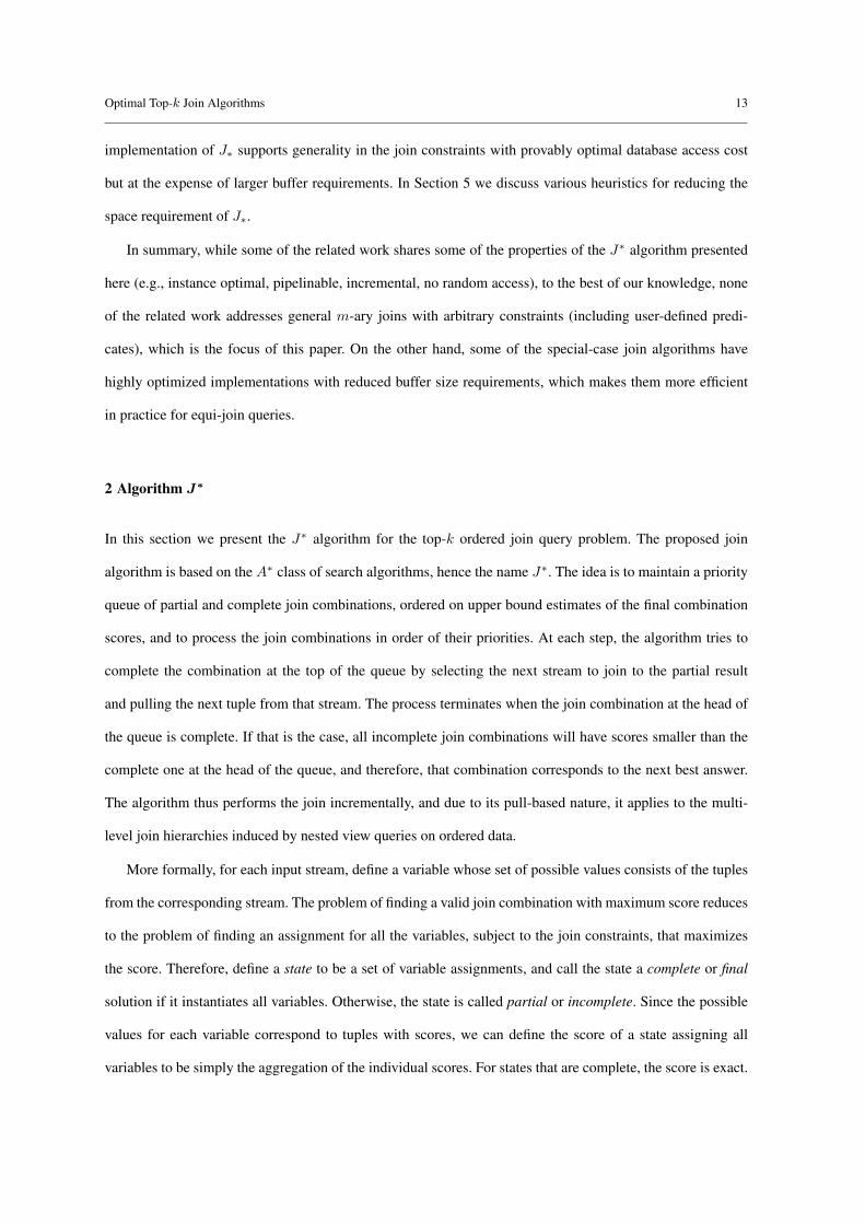
2 Algorithm J∗
In this section we present the J∗ algorithm for the top-k ordered join query problem. The proposed join
algorithm is based on the A∗ class of search algorithms, hence the name J∗. The idea is to maintain a priority
queue of partial and complete join combinations, ordered on upper bound estimates of the final combination
scores, and to process the join combinations in order of their priorities. At each step, the algorithm tries to
complete the combination at the top of the queue by selecting the next stream to join to the partial result
and pulling the next tuple from that stream. The process terminates when the join combination at the head of
the queue is complete. If that is the case, all incomplete join combinations will have scores smaller than the
complete one at the head of the queue, and therefore, that combination corresponds to the next best answer.
The algorithm thus performs the join incrementally, and due to its pull-based nature, it applies to the multi-
level join hierarchies induced by nested view queries on ordered data.
More formally, for each input stream, define a variable whose set of possible values consists of the tuples
from the corresponding stream. The problem of finding a valid join combination with maximum score reduces
to the problem of finding an assignment for all the variables, subject to the join constraints, that maximizes
the score. Therefore, define a state to be a set of variable assignments, and call the state a complete or final
solution if it instantiates all variables. Otherwise, the state is called partial or incomplete. Since the possible
values for each variable correspond to tuples with scores, we can define the score of a state assigning all
variables to be simply the aggregation of the individual scores. For states that are complete, the score is exact.

14 Apostol (Paul) Natsev et al.
GETNEXTMATCH():
1 if (queue.EMPTY()) then
2 return NULL
3 endif
4 head ← queue.POP()
5 if (head .COMPLETE()) then
6 return head
7 endif
8 head2 ← head .COPY()
9 head2 .ASSIGNNEXTMATCH()
10 if (head2 .VALID()) then
11 queue.PUSH(head2 )
12 endif
13 head .SHIFTNEXTMATCH()
14 queue.PUSH(head)
15 Goto Step 1
SHIFTNEXTMATCH():
1 child ← GETNEXTUNASSIGNED()
2 child .match ptr ++
3 if (child .match ptr == NULL ) then
4 child .match ptr ←5 child .GETNEXTMATCH()
6 endif
ASSIGNNEXTMATCH():
1 child ← GETNEXTUNASSIGNED()
2 child .match ptr ++
3 if (child .match ptr == NULL ) then
4 child .match ptr ←5 child .GETNEXTMATCH()
6 endif
7 Make child an assigned node.
Fig. 2 Pseudo-code for the J∗ join algorithm. The three functions above form the crux of the algorithm.
For incomplete states, the score can be upper bounded by exploiting the monotonicity of the score aggregation
function. Since all tuples are scanned in decreasing order of their scores, we can simply take the score value
of the previous item as an upper-bound estimate of the next score for a particular variable. We then define the
state potential to be the maximum score a solution can take if it agrees with all assignments in the given state.
The state potential can be computed by upper bounding the scores of all non-instantiated variables for a given
state.
We note that the above-defined potential can be expressed as a combination of the exact gain for reaching
the given state (computed from the instantiated variable scores) and the upper-bounded potential of reaching
a terminal solution from the given state (computed from the score upper bounds on the free variables). There-
fore, the search problem can be stated as an A∗ problem instance, and can be solved efficiently by processing
states in decreasing order of their potential. When the potentials of two states are equal, we order them accord-
ing to the number of instantiated variables, and if those numbers are equal as well, we break ties randomly.
This extra tie-breaking mechanism ensures that given the same potential, we would consider more complete
states before less complete ones, and it is used in proving the optimality results in Section 6.

Optimal Top-k Join Algorithms 15
The pseudo code for the crux of the algorithm is listed in Figure 2. In order to output the top k matches,
the algorithm invokes the GetNextMatch() routine k times. During the main processing loop, the algorithm
simply takes the head of the queue, selects one unassigned variable (i.e., picks the next stream to join to the
partial result), and expands the old state into two new states. The first one is identical to the original state,
except that the chosen variable is now assigned to the next possible match. The second one leaves that variable
unassigned but shifts the pointer to the next possible value so that the last assignment is not considered again.
This is necessary so that the algorithm can later back track and consider the other possible values for that
variable. Both new states are inserted back into the priority queue according to their new score estimates but
only if they satisfy the join constraints.
The pseudo code in Figure 2 is fairly self-explanatory, with the exception of a few variables and subrou-
tines. The queue variable denotes the priority queue for the corresponding join query; and the match ptr is
simply a pointer to the next possible match for a given sub-query. The priority queue supports standard opera-
tions Pop(), Push(), and Empty(). The query/view nodes have methods Copy(), Complete() (for checking if a
state is complete), Valid() (for checking if a state meets the join constraints), GetNextUnassigned() (for select-
ing the next variable for assignment), and the methods listed in Figure 2: GetNextMatch(), ShiftNextMatch(),
and AssignNextMatch(). The GetNextUnassigned() routine encapsulates a heuristic that controls the order
in which free variables are assigned. In general, we want to select the variable that will provide the largest
refinement on the state potential, because the tighter the score upper bounds are, the faster the algorithm will
converge to a solution. Examples of possible heuristics include selecting the variable that is most constrained
or least constraining given the join predicates; the variable that could lead to the largest drop in the state po-
tential; or the variable that is expected to lead to the largest drop.2 In general, a heuristic that quickly reduces
ambiguity in the partial solution should lead to faster convergence to the best solution, and the rate at which
ambiguity is reduced by different heuristics can be measured empirically.
One important property to note from the pseudo-code is the recursive invocation of method GetNextMatch()
from methods ShiftNextMatch(), and AssignNextMatch(). This illustrates why the algorithm works well on
2 The last heuristic can be implemented by comparing the variable weights and their score distribution gradients. This obser-
vation was made in [14], where the authors achieved significant speedup for skewed score distributions using the same technique.
They computed the weight by taking a derivative of the score aggregation function with respect to the given stream score, and
approximated the gradient with a score difference.
16 Apostol (Paul) Natsev et al.
join hierarchies—when computing the next best match for a join at level l, the algorithm recursively invokes
the same subroutine for some of the children at level l+1, where increasing levels correspond to deeper levels
in the tree. This recursive mechanism enables nested joins/views to be processed efficiently. The efficiency
comes from the fact that the recursive call is executed only as needed, using a pull-based model.
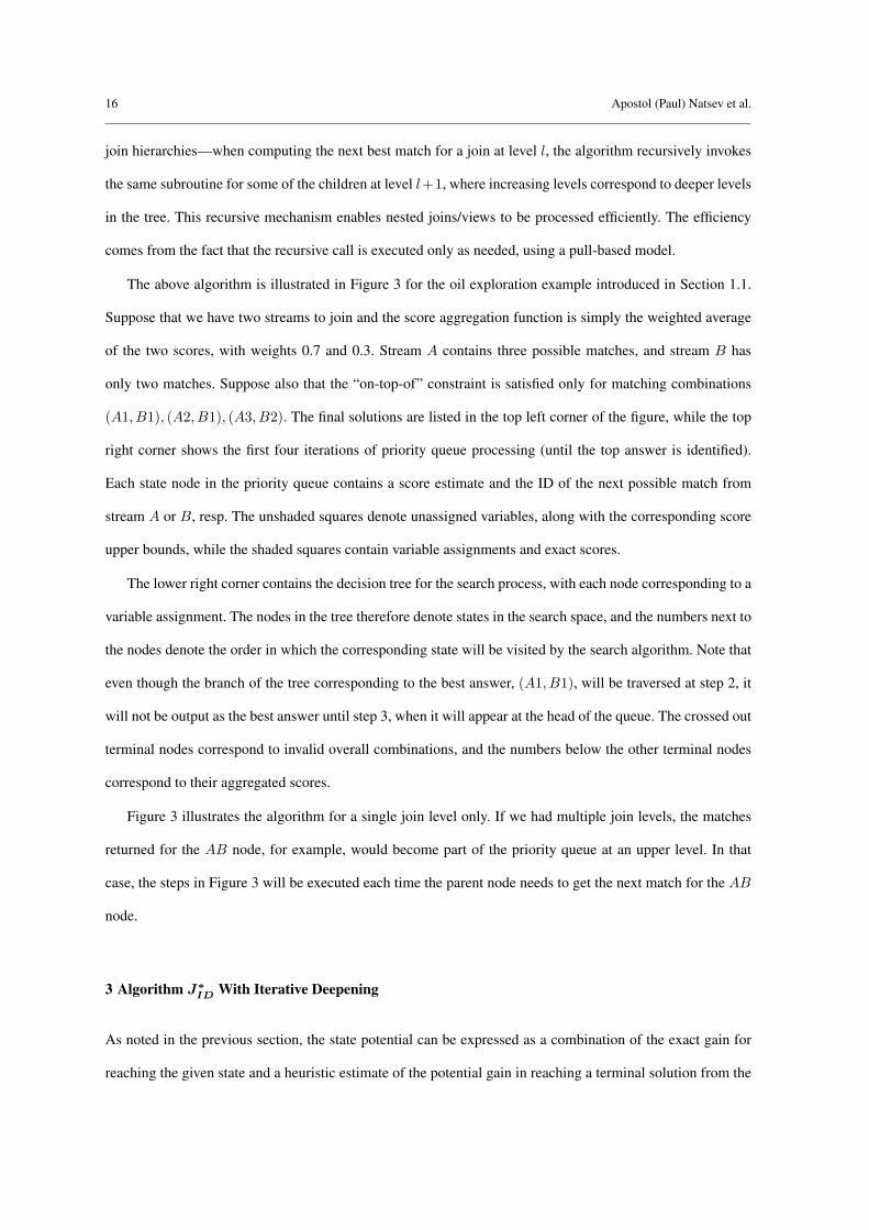
The above algorithm is illustrated in Figure 3 for the oil exploration example introduced in Section 1.1.
Suppose that we have two streams to join and the score aggregation function is simply the weighted average
of the two scores, with weights 0.7 and 0.3. Stream A contains three possible matches, and stream B has
only two matches. Suppose also that the “on-top-of” constraint is satisfied only for matching combinations
(A1, B1), (A2, B1), (A3, B2). The final solutions are listed in the top left corner of the figure, while the top
right corner shows the first four iterations of priority queue processing (until the top answer is identified).
Each state node in the priority queue contains a score estimate and the ID of the next possible match from
stream A or B, resp. The unshaded squares denote unassigned variables, along with the corresponding score
upper bounds, while the shaded squares contain variable assignments and exact scores.
The lower right corner contains the decision tree for the search process, with each node corresponding to a
variable assignment. The nodes in the tree therefore denote states in the search space, and the numbers next to
the nodes denote the order in which the corresponding state will be visited by the search algorithm. Note that
even though the branch of the tree corresponding to the best answer, (A1, B1), will be traversed at step 2, it
will not be output as the best answer until step 3, when it will appear at the head of the queue. The crossed out
terminal nodes correspond to invalid overall combinations, and the numbers below the other terminal nodes
correspond to their aggregated scores.
Figure 3 illustrates the algorithm for a single join level only. If we had multiple join levels, the matches
returned for the AB node, for example, would become part of the priority queue at an upper level. In that
case, the steps in Figure 3 will be executed each time the parent node needs to get the next match for the AB
node.
3 Algorithm J∗ID With Iterative Deepening
As noted in the previous section, the state potential can be expressed as a combination of the exact gain for
reaching the given state and a heuristic estimate of the potential gain in reaching a terminal solution from the

Optimal Top-k Join Algorithms 17
……IDIDScoreScore
matchesmatches
……110.900.90
……0.600.60 22
……110.900.90
……IDIDScoreScore
matchesmatches
……0.800.80 22
……330.700.70
On top ofAA BB
ABAB
111.01.0 11
BBAAScoreScore
110.930.93 11
BBAAScoreScore
220.930.93 11
220.860.86 11
BBAAScoreScore
110.900.90 11
110.900.90 22
330.860.86 11
220.930.93 11
BBAAScoreScore
110.900.90 11
110.900.90 22
0.830.83 22 11 ……
220.670.67 33 ……
110.900.90 11 ……
BBAAScoreScore
matchesmatches
……
0.7 0.3
Step 0 Step 1 Step 2 Step 3Output stream AB
Input stream A Input stream B
Assignments priority queue
Fig. 3 Illustration of the J∗ algorithm for query: Find occur-
rences of rock texture A on top of rock texture B. The indi-
vidual matches for each query are shown in a table next to the
corresponding view node. The matches for the root query are
derived from the matches of the two children. The first few
steps of the process are illustrated to the right by showing the
priority queue at each of the steps.
ALGORITHM J∗ID():
1 Let queue(r) be the priority queue at round r
2 r ← 1
3 queue(1)← root state
4 while (queue(r).head 6= NULL and
5 !queue(r).head .COMPLETE())
6 do
7 if (∃ free variable at depth < (r + 1)s) then
8 process that variable
9 else
10 move queue(r).head into queue(r + 1)
11 endif
12 endwhile
13 if (queue(r).head 6= NULL ) then
14 move queue(r).head into queue(r + 1))
15 endif
16 r ← r + 1
17 if (queue(r).head == NULL or
18 queue(r).head .COMPLETE()) then
19 return queue(r).head
20 else
21 Goto Step 4
22 endif
Fig. 4 Pseudo-Code for the J∗ID algorithm.
given state. By processing states in decreasing order of their potential, J∗ automatically inherits all properties
of an A∗ algorithm.3 As long as the heuristic gain approximation never underestimates the true gain (i.e., the
potential is always upper-bounded), A∗ algorithms are guaranteed to find the optimal solution (i.e., the one
with maximum gain) in the fewest number of steps (modulo the heuristic function). Therefore, they provide a
natural starting point for many search problems [26].
3 A∗ algorithms form a class of search methods that prune the search space by taking into account the exact cost of reaching
a certain state and a heuristic cost approximation of reaching a solution from the given state (see, for example, [26]).

18 Apostol (Paul) Natsev et al.
A∗ algorithms, however, are designed to minimize the number of processed states, not the database ac-
cess cost from our cost model. Minimizing the access cost translates into minimizing the number of values
considered for each variable assignment, and is not necessarily optimized by A∗ algorithms. In addition, A∗
algorithms suffer from large space requirements (exponential in the worst case), which also makes them less
suitable in practice. In this section, we address both of the above issues by incorporating iterative deepening
into J∗.
Iterative deepening is a mechanism for limiting computational resources by dividing computation into
successive rounds. Each round has an associated cut-off threshold, called depth here, which identifies the
round’s boundaries. The depth threshold is defined on some attribute, and computation in each round continues
as long as the value of that attribute is below the specified threshold. At the end of a round, if a solution has
not been found, the algorithm commences computation in the next round. Iterative deepening can therefore
be applied to a variety of algorithms by specifying the depth attribute and the threshold bounds for each
round. Solution correctness and optimality are guaranteed as long as the modified algorithm can guarantee
that solutions in earlier rounds are better than the ones in later rounds.
For our purposes, we can define the depth of an algorithm to be the maximum number of objects scanned
via sequential (sorted) access in any of the streams. We can define the depth of a state in a similar fashion, by
counting the maximum number of objects considered for each variable in the given state. This definition for
depth is very natural given that the cost of the J∗ algorithm is directly proportional to the number of scanned
objects. We can further define the ith round to include all computation from depth i · s to depth i · s + s− 1,
inclusive, for some constant step factor s ≥ 1. The step factor is needed to limit both access cost and space
requirements in some worst cases, and can be used to control a trade-off between the two. The pseudo-code
for the modified J∗ algorithm with iterative deepening is illustrated in Figure 4. Intuitively, the algorithm
processes all states in a given round until a solution is found or there are no more valid states to process in
that round. Meanwhile, the algorithm maintains a second priority queue (associated to the next round) of all
states that cannot be refined further in the current round since all of their free variables have reached the depth
of the next round. If at the end of a round a solution was found, it is inserted in the priority queue for the next
round. If it turns out to have the highest potential in the priority queue, this solution is returned as the next
best answer. Otherwise, computation for the next round commences.

Optimal Top-k Join Algorithms 19
Algorithm J∗PA:
1. Let P be the set of join predicates
2. Call a state α eligible if ∀ non-instantiated stream T ,
∃ a key predicate p ∈ P :
(a) There is an index I defined on T
(b) target(p) is a key column in I
(c) bound(p) is invariable given state α
3. sorted cost(α) ≡ sorted cost when α reached
4. predicate cost(α) ≡ predicate cost when α reached
5. credit(α) ≡ sorted cost(α)− predicate cost(α)
6. cost(α) ≡∑p∈P
Cp · filter factor(p) ·N
7. Run modified J*:
If head is eligible and cost(head) ≤ credit(t), then
(a) Expand head by predicate access
(b) Insert resulting states into the priority queue
Fig. 5 Pseudo-code for the J∗PA join algorithm.
Algorithm ε-J∗ (resp., ε-J∗PA):
1. Let ε ≥ 0 be a user-specified parameter.
2. Let U(k, t) be kth largest potential in the priority queue
of J∗ (resp., J∗PA) at time t (i.e., U(k, t) is an upper
bound on the score of the kth best join combination). Let
U(k, t) = 1.0 if the priority queue has < k states at time t.
3. Let L(k, t) be the kth largest potential of a complete state
(i.e. solution) in the priority queue of J∗ (resp., J∗PA) at
time t (i.e., L(k, t) is a lower bound on the score of the kth
best join combination). Let L(k, t) = 0.0 if the priority
queue does not have k complete states at time t.
4. Run J∗ (resp., J∗PA) algorithm until time t∗
such that: U(k, t∗) ≤ (1 + ε)L(k, t∗).
5. Output the k complete solutions with scores≥ L(k, t∗).
Fig. 6 Pseudo-code for the ε-J∗ join algorithm.
The above algorithm can be trivially generalized to output the top k best answers rather than just the single
best answer. In that case, the algorithm would run in each round until it finds the k best solutions for that round
or it exhausts all possible combinations up to the corresponding depth. Alternatively, when outputting results
one at a time, without knowing the desired number of outputs, the algorithm would have to keep track of the
states in the priority queue in each round and cycle through the rounds until the next best solution is found.
4 Algorithm J∗P A
The algorithm from the previous section uses only sequential access when scanning the input streams. How-
ever, depending on the selectivity of the join predicates, it may be much more efficient to perform a predicate
access if the system can exploit an index to return the objects that satisfy a given predicate. An extreme case
is the random access scenario considered by Fagin [10], where each object participates in exactly one valid
join combination (i.e., the probability of an arbitrary combination satisfying the join predicates is 1Nm−1 ). In
that case, using random access to complete partial join combinations is much more efficient than scanning in
sorted order until the join constraints are met.

20 Apostol (Paul) Natsev et al.
We therefore propose a variation of the algorithm that can exploit indexes to complete states via predicate
access. The pseudo-code appears in Figure 5. The algorithm works like the J∗ algorithm with one modifica-
tion. When processing an an incomplete state from the head of the priority queue, the algorithm first checks
whether the state is instantiated sufficiently to allow completion by predicate access. If that is the case, the
algorithm can process the state via predicate access rather than sorted access, provided the estimated cost of
the predicate access is not too large. Note that each state processed via predicate access will be expanded
into a number of new states (corresponding to all join combinations involving the returned objects from the
uninstantiated streams). Therefore, we perform the predicate access only if the estimated number of returned
objects is sufficiently small (i.e., smaller than a certain threshold). The threshold is determined dynamically
by the difference in sorted access cost vs. predicate access cost at that point in time.4 The cost of a predicate
access query (i.e., the number of returned objects) can be estimated with traditional selectivity estimation
techniques (e.g., random sampling or histogram statistics). The decision on when to use predicate access can
be based on traditional query optimization techniques. For example, given a set of random access indexes and
a set of key predicates that can be used to filter out results, the system can estimate the filter factors (or the
selectivity) of each predicate and choose the one with the smallest filter factor (highest selectivity).
5 Approximation Algorithms
Both algorithms J∗ and J∗PA solve the top-k query problem exactly. The J∗PA algorithm achieves better perfor-
mance by relaxing the requirement for using only sorted access but still does not compromise the correctness
of the results. In some scenarios, however, the user may be willing to sacrifice algorithm correctness for im-
proved running times or smaller memory footprint. In the following, we describe variations that reduce the
cost of the algorithm by approximating the optimal answer. In particular, we describe a variation for each
of the above algorithms that provides approximations with provable bounds. We also describe a variety of
other approximation heuristics that impose restrictions on the length of the priority queue or on the minimum
required potential in the queue.
4 This heuristic essentially balances the two (negatively correlated) types of access cost in an effort to minimize the overall
access cost. In [13], the authors present a hybrid algorithm, called CA, that balances sorted access cost with random access cost.
Under certain assumptions, they prove optimality results independent of the unit costs for sorted access and random access. We
believe that our algorithm has similar behavior.

Optimal Top-k Join Algorithms 21
Intuitively, we call an algorithm ε-admissible, or an ε-approximation, if it returns solutions that can be
worse than optimal by at most ε. More formally, we adopt the definition from [13], and we say that an
algorithm provides an ε-approximation to the top-k ranked join problem if it returns a set R of k solutions
such that:
∀x ∈ R, y /∈ R : (1 + ε) · x.score ≥ y.score.
Figure 6 illustrates the modified J∗ and J∗PA algorithms that return an ε-approximation for a user-specified ε.
Alternatively, the algorithms can be modified to output the current approximation factor (ε = (U(k, t) −
L(k, t))/L(k, t)) at any given time t, and the user can decide when to stop the algorithm interactively. Note
that for ε = 0, both of the approximation versions behave exactly as the original algorithms and output the
best k solutions. One can therefore think of the modified versions as progressive algorithms that gradually
refine their solutions.
In the following, we describe several approximation heuristics that are expected to reduce both the space-
and access-cost of the algorithm by limiting the priority queue size and approximating the optimal answer if
necessary. The performance of the greedy first-k heuristic is also studied empirically in Section 7.
– first-k—greedy approximation version of J∗, which runs until there are k complete and valid join combi-
nations, and then outputs them as the best solutions, even if they are not at the top of the priority queue.
This corresponds to running the ε-J∗ algorithm and stopping at the earliest possible time (i.e, for any ε
approximation factor that is not ∞) in order to produce the coarsest possible approximation with that
algorithm.
– max length—this heuristic limits the maximum size of the priority queue to a certain fixed threshold τ .
With this heuristic, if the queue grows longer than τ after an insertion, it will be truncated by dropping
the items at the end (i.e., with smallest score estimates). The threshold may be set globally or can be
query-specific. For example, it may be a function of the number k of desired answers, estimating the ex-
pected number of matches to be scanned from each stream. This heuristic bounds the worst-case memory
requirements without affecting typical (or average case) scenarios. It will lead to approximations only if
the size threshold is set very aggressively or if the join constraints are very harsh.
– min score—heuristic that allows the queue length to vary so long as all the assignments in the queue
have score estimates above a certain threshold τ . Again, the score cut-off threshold may vary for different

22 Apostol (Paul) Natsev et al.
queries but would be fixed within a single query. This heuristic can lead to more memory-efficient exe-
cution (i.e., shorter queue length) in typical cases and better approximations (although with higher space
requirements) in atypical cases (e.g., harsh join constraints).
– max range—heuristic that limits the range of scores between the first and last item in the queue to be
less than a certain threshold τ . This is similar to the above heuristic but it sets the cut-off score threshold
relative to the current top score. This can compensate for skewed distributions where the score estimates
can drop rapidly.
– max ratio—heuristic that limits the ratio between the scores of the first and last item in the queue to be
less than a certain threshold τ . This is similar to the previous heuristic but it considers the relative score
difference rather than the absolute one (e.g., drop assignments with scores smaller than 1% of the top
score).
– dynamic thresholding—more complicated counterparts for the above heuristics, where the thresholds vary
in accordance to run-time statistics, selectivity estimation, or other methods for dynamic threshold esti-
mation. Those may include estimates on the number of items that will need to be scanned from each
stream using average case analysis and assumptions on the score distributions. Another approach may be
to convert the top-k query into a score range query using distribution statistics and selectivity estimation
techniques from [4,7,5].
6 Optimality
In this section, we consider the performance of the proposed algorithms in terms of their database access cost,
or cardinality of input tuples. We use the notion of instance optimality, defined by Fagin et al. in [13]:
Definition 61: Let A be a set of algorithms that solve a certain problem, and let D be a set of valid inputs
for that problem. Let cost(A,D) denote the cost of running algorithm A ∈ A on input D ∈ D. We say that
algorithm B ∈ A is instance-optimal over A and D if ∀A ∈ A and D ∈ D, ∃ constants c and c′ such that:
cost(B, D) ≤ c · cost(A,D) + c′.
The constant c is called the optimality ratio of B.
As discussed in [13], the above notion of optimality is very strong if A and D are broad. Intuitively, if
an algorithm is instance-optimal over the class of all algorithms and all inputs, that means that it is optimal

Optimal Top-k Join Algorithms 23
in every instance, not just in the worst case or the average case. Given the above definition, we can state the
following theorem:
Theorem 62: Let A be the set of all algorithms that solve the top-k ranked join problem using only sequential
(sorted) access. Let D be the set of all valid inputs (i.e., database instances) for that problem. Then, algo-
rithm J∗ with Iterative Deepening is instance-optimal over A and D with respect to database access cost.
Furthermore, it has an optimality ratio of m, where m is the number of streams being joined, and no other
algorithm has a lower optimality ratio.
Proof: Let A ∈ A be an arbitrary algorithm that solves the ranked join problem using only sorted access.
Let D ∈ D be an arbitrary database instance for the problem. For simplicity, and without loss of generality,
assume that each round in algorithm J∗ with Iterative Deepening is defined as running at strictly consecutive
depths (i.e., the step of incrementing the depth at each round is exactly 1). Also, let the J∗ algorithm terminate
at depth d after outputting the best k answers. We will show that algorithm A terminates at depth ≥ d.
For as proof, suppose that A terminates at some depth dA < d. Therefore, there must be k valid solutions
by depth dA ≤ d− 1. Since J∗ inherits all the properties of an A∗ algorithm within each round of processing,
it follows that J∗ is complete and optimal with respect to the scoring function. In other words, J∗ would have
seen the k best solutions, if k solutions exist, by depth d − 1. Since we know that these solutions exist, J∗
must finish the round at depth d − 1 with k valid solutions of maximum score until that round. The fact the
algorithm proceeds to run in round d, however, and does not terminate at round d− 1, means that there was a
partial state at depth d which appeared before some of the k valid solutions in the priority queue at depth d.
Let β be the kth best solution until depth d−1, and let α be a partial state at depth d such that potential(α) > potential(β)
(α exists since the algorithm didn’t terminate after round d−1). We note that the above potential inequality is
strict due to the tie-breaking mechanism we introduced in Section 2. If the two states had equal potential, the
tie-breaking mechanism would order β before α since β is a complete solution, and α is incomplete. If that
were the case, the algorithm would have terminated after round d− 1. Since it didn’t, there must be a state α
with a potential strictly bigger than that of β.
Now, since α was inserted in the priority queue at some point, it means that the partial instantiations in
it do not invalidate the join predicates. Therefore, we can construct a complete and valid state γ that agrees
with α on all of its instantiations through depth d − 1, and assigns scores to the non-instantiated variables at

24 Apostol (Paul) Natsev et al.
depth d as follows. For each of the non-instantiated variables by depth d, γ takes the score at depth d− 1 for
that variable (the last value seen for that variable by depth d−1, inclusive). In other words, we take the partial
state α and complete it at depth d by assigning the maximum possible scores at that depth. All attributes
other than the score are identical to those of α on the instantiated variables and are assigned arbitrarily for the
non-instantiated variables to satisfy the join predicates.
Now, consider a database instance D′, which is equivalent to D on all values up to depth d − 1, and
contains the same values at depth d as in depth d − 1 for all non-instantiated variables in α. Since the two
databases are identical through depth d−1, algorithm A would perform identically on both and will therefore
terminate by depth d − 1 on database D′ by outputting the same top k answers, with β being the kth best
answer. However, consider the newly introduced γ combination. It is complete at depth d, it is valid, and by
construction, its score is equal to the potential of α. Therefore,
score(γ) = potential(α) > potential(β) = score(β),
where the two equalities follow from the fact that states γ and β are complete. We therefore have a valid
solution that has a score higher than the kth best score output by A. Now, since γ was at least partially
instantiated at depth d, it follows that it could not have been seen by algorithm A, which considers solutions
only up to depth dA < d. Therefore, algorithm A could not have output γ as one of the best k solutions, which
would be an error.
Since algorithm A ∈ A is correct, it follows that our assumption that it terminates before depth d was
wrong. Therefore, algorithm A would have to scan at least d objects in at least one of the streams, and its cost
will be higher than d. But the cost of J∗ is at most md since it terminates at depth d and it therefore scans at
most d objects from each of the m streams. Thus, we have shown that
cost(J∗, D) ≤ m · cost(A, D), ∀A ∈ A, ∀D ∈ D
and therefore algorithm J∗ with Iterative Deepening is instance optimal over A and D, with optimality ratio
of m.
The lower bound on the optimality ratio was proved by Fagin et al. in [13] for a special case of the top-k
ranked join problem. Since no algorithm can have a smaller optimality ratio than m for that special case, it
follows that the same claim holds for the more general case. Therefore, algorithm J∗ with Iterative Deepening
has the best optimality ratio.

Optimal Top-k Join Algorithms 25
Similarly to the exact ranked join problem, we can formulate the equivalent result for the ε-J∗ algorithm
for the approximate ranked join problem:
Theorem 63: LetA be the set of all algorithms that output an ε-approximation to the top-k ranked join problem
using only sorted access. Let D be the set of all valid inputs (i.e., database instances) for that problem. Then,
algorithm ε-J∗ is instance-optimal over A and D with respect to total sorted access cost. Furthermore, it has
an optimality ratio of m, where m is the number of streams being joined, and no other algorithm has a lower
optimality ratio.
Proof: The proof is very similar to that of Theorem 61 with the modification that potential(α) > (1 + ε)potential(β).
The lower bound for the optimality ratio follows directly from the corresponding claim in Theorem 61 since
that is a special case of the ε-approximation ranked join problem.
We do not have matching optimality results for the predicate access case (i.e., algorithms J∗PA and ε-J∗PA)
due to the increased complexity of adding arbitrary join predicates and index exploitation. However, if we
restrict our attention to the special case of random access only (i.e., each join predicate is the equivalence re-
lation on a key attribute), we believe that some of the results pertaining to the Combined Algorithm from [13]
will carry over to the restricted version of J∗PA. In general, if we can guarantee that each key predicate will
generate only a constant number of outputs by probing the index, then the cost of each predicate access will
be proportional to that of a sequential access, and the total cost will be proportional to the sequential access
cost.5 In the most general case, when the above assumption does not hold, the heuristic of balancing the sorted
access cost with that of predicate access is designed to achieve the same behavior as in the above scenarios.
The performance there, however, is dependent on the quality of the selectivity estimation procedure.
7 Empirical Evaluation
In this section we describe simulation experiments for evaluating the proposed algorithms. We implemented
the algorithms as part of a constrained query framework that we proposed in [25]. The entire framework is
about 5000 lines of C++ code and provides an API for plugging arbitrary attributes, constraints, and join5 An example of the above scenario might be combining image regions under a set of spatial constraints. If each image
is decomposed into at most a constant number of regions, then by instantiating a single region and fixing its image ID, we
automatically limit the number of valid join combinations to a constant number.

26 Apostol (Paul) Natsev et al.
algorithms. All of the experiments were run on an IBM ThinkPad T20, featuring a Pentium III 700 MHz
processor, 128 MB RAM, and running Linux OS. All of the experiments we report use synthetic data sets,
generated to model real data.
The queries were generated pseudo-randomly by having a fixed query tree structure but with random
parameters, such as attribute values for the join predicates, node scores, and node weights. Each query was
built as a tree joining m leaf nodes, where each leaf node had n matches. Each node performed an equi-join of
its children views over a fixed attribute. The attribute values were generated randomly from an integer range
that controls the probability that the join constraint is satisfied. Unless otherwise noted, we used probability of
0.5, in order to model general relational binary predicates (e.g., left-of/right-of, above/below, smaller/bigger,
before/after, etc). Also, unless specified otherwise, children nodes had weights distributed uniformly in the
[0,1] range and scaled to add up to 1. For the scores of matches at the leaf nodes (i.e., atomic queries), we
considered the following distributions: uniform (i.e., linear decay), exponential decay, sub-linear decay, and
the i%-uniform distributions from [14], for i = 1, 0.1, and 0.05. The i%-distributions were designed in [14]
to model real image data and consist of i% of all scores being uniformly distributed in the [0.5, 1] range (i.e.,
medium and high scores), while the rest are all below 0.1 (i.e., insignificant scores).
The parameters m, p, n, and the desired number of answers k for each query, are specified for each
experiment. Default values are m = 3, p = 0.5, n = 10000, k = 30, and 1%-uniform score distributions. We
performed experiments to answer the following questions:
– How does constraint probability affect performance?
– How does query tree size affect performance?
– How does number of outputs affect performance?
– How does database size affect performance?
– How does weight distribution affect performance?
– How does score distribution affect performance?
To evaluate the performance of a query, we measured the number of tuples scanned by the algorithm, as well
as the maximum size of the priority queue. The first measure is the database access cost (proportional to the
running time) of the algorithm, while the second corresponds to the space requirements of the algorithm. All

Optimal Top-k Join Algorithms 27
of the results we report are averaged values over 10 random queries of the given type. The results are listed in
Figures 7–10.
The first set of experiments studies the dependence of the algorithm on the probability that the join con-
straints are met. The join constraints’ probabilities were modeled by assigning a random attribute with d
possible values to each node, and using pairwise join constraints that require the attributes to have the same
value. We varied d from 1 to 30, thus obtaining probabilities p = 1/d from 0.03 to 1.0. The results are plotted
in Figures 7(a) and 7(b) for three different weight distribution cases—uniform, decaying, or equal weights.
Figure 7(a) shows almost identical database access cost for all three cases, which means that the running time
of the algorithm is fairly robust with respect to the weight distribution. Figure 7(b), however, shows that in
the case of equal weights, the algorithm has a higher space requirement. This is to be expected since in that
case the algorithm cannot exploit the weights to scan “more important” streams first, and will therefore take
longer to converge to the optimal solution. Overall, both figures show that for reasonable values of p, when
there are enough valid combinations to generate the desired number of outputs, both the database access cost
and the space requirements are almost constant.
The second set of experiments evaluated the performance of the algorithm with respect to the size of the
query tree. Given the number of streams to join, we considered two types of queries. The first was flat queries
joining all input streams in a single level (denoted as max-width queries). The second were nested max-height
queries that join the same number of streams but only two at a time, by building a balanced binary tree on
the input streams. Figures 8(a)–8(b) show the performance of both types of queries with otherwise identical
parameters, and with varying number of streams to join. Note also that we used larger streams (100000 tuples)
in these queries in order to test scalability with respect to database size. We can make several conclusions from
the figures. First, despite the increased database size, both types of queries scan only a small number of tuples
that appears to be dependent on the desired number of outputs only and not on the database size. And second,
all else being equal, nested queries are more costly than flat queries in terms of access cost but cheaper in
terms of space requirements. The higher access cost can be explained by the fact that the number of possible
matches increases exponentially at each level in the nested queries. Yet, the difference in the access cost is
not significant, which shows that the algorithm is efficient even for such highly-nested joins.

28 Apostol (Paul) Natsev et al.
The third set of experiments was designed to evaluate the dependence of the algorithm on different score
distributions. We considered the six distributions described earlier and computed access cost and space re-
quirements for varying number of desired outputs, k. The results in Figures 9(a) and 9(b) generally show a
sub-linear dependence on k.6 An exception is the exponentially decaying score distribution, where the dif-
ference between successive score values becomes negligible very quickly and the algorithm takes longer to
converge due to fact that successive assignments lead to very small refinements in the overall solution score.
However, this trend is reversed for space requirements in Figure 9(b), where quickly decaying distributions
require less space. This could also be explained by the theory that quickly decaying scores lead to small re-
finements in the score estimates very quickly, and therefore the algorithm is more likely to be localized to the
same set of assignments, as opposed to spreading its computation over a large set of assignments.
The final experiment measured the performance of the simple first-k greedy approximation algorithm as
compared to the original J∗ algorithm (see Section 5). We measured the database access cost and total space
requirements of the greedy J∗ version as a fraction of the corresponding values for J∗. We also calculated the
recall and precision values. We considered the output of the J∗ algorithm for a top-k query to be the ground
truth for that query, and therefore, each top-k query had exactly k correct answers. Thus, the precision, defined
as the fraction of output answers that were correct, is the same as the recall, or the fraction of correct answers
retrieved by the approximation algorithm.
The recall, relative access cost and relative space cost are shown as percentages in Figure 10. From the
recall curve in the graph, we can conclude that the greedy heuristic is an excellent approximation to the
optimal answers for values of k that are not very small. We hypothesize that the greedy algorithm outputs
the tuples in a slightly different order, which reduces the recall at the beginning. However, the identities of
the top-k tuples eventually match the true answers, even though they might be shuffled somewhat. Thus, the
unordered set of top-k answers is approximated very well. In addition, we see that the database access cost
is reduced by 5–10%, while the space requirements are reduced by 40%. Therefore, we can conclude that the
greedy first-k heuristic provides significant cost savings with almost no reduction of accuracy.
Based on the results we have reported, we can conclude the following:
6 Note that the number of scanned database tuples can be smaller than the number of desired outputs. This is due to the fact
that each tuple can participate in multiple valid join combinations.

Optimal Top-k Join Algorithms 29
– J∗ is fairly robust with respect to weight distributions but it can take advantage of unequally weighted
queries to reduce space requirements.
– J∗ scales very well with respect to database size and desired number of outputs.
– J∗ scans more inputs but takes less space as the rate of score decay increases.
– J∗ scales well with respect to query tree size.
– J∗ performs efficiently on nested queries.
– The greedy first-k heuristic provides significant cost savings with almost no drop in accuracy of the results.
8 Conclusions
In this paper, we introduced several algorithms for incremental joins of ranked inputs based on user-defined
join predicates. The algorithms enable optimization of complex queries by providing the ability to integrate
result sets from multiple atomic independent queries, using user-defined criteria for integration. The need for
efficient ranked query aggregation and optimization arises naturally in domains dealing with ordered inputs
and multiple ranked data sets, and requiring the top k solutions. These include multimedia query systems, as
well as traditional database applications involving optimal resource allocation, scheduling, decision making,
tournament/itinerary/portfolio ranking, etc.
Our proposed J∗ algorithm differs from previous work in two main aspects: 1) it can support joins of
ranked inputs based on user-defined join predicates; and 2) it can be pipelined into multi-level joins. We also
presented a J∗PA version of the algorithm that uses predicate access to reduce the cost of the algorithm, and
presented variations of both algorithms that reduce complexity by approximating the solution. The proposed
class of algorithms are the only ones to the best of our knowledge that support general ranked joins with
user-defined join constraints. We proved strong optimality results for some of the algorithms, and performed
an extensive empirical study for their validation in practice.

30 Apostol (Paul) Natsev et al.
References
1. Bruno, N., Chaudhuri, S., Gravano, L.: Top-k selection queries over relational databases: Mapping strate-
gies and performance evaluation. ACM Trans. Database Syst. (TODS) 27(2), 153–187 (2002). DOI
http://doi.acm.org/10.1145/568518.568519
2. Carey, M., Kossmann, D.: Reducing the braking distance of an SQL query engine. In: Proc. of the 1998 Intl. Conference on
Very Large Databases (1998)
3. Chang, K.C.C., Hwang, S.W.: Minimal probing: supporting expensive predicates for top-k queries. In: SIG-
MOD ’02: Proc. ACM SIGMOD Intl. Conf. on Management of Data, pp. 346–357. Madison, WI (2002). DOI
http://doi.acm.org/10.1145/564691.564731
4. Chaudhuri, S., Gravano, L.: Optimizing queries over multimedia repositories. In: Proc. ACM-SIGMOD Intl. Conference on
Management of Data (SIGMOD ’96), pp. 91–102. Montreal, Canada (1996)
5. Chaudhuri, S., Gravano, L.: Evaluating top-k selection queries. In: Proc. of the 25th Intl. Conference on Very Large
Databases (VLDB ’99), pp. 399–410. Edinburgh, Scotland (1999)
6. Croft, W.B.: Combining approaches to information retrieval. Advances in Information Retrieval. Kluwer Academic Pub-
lishers (2000)
7. Donjerkovic, D., Ramakrishnan, R.: Probabilistic optimization of top N queries. In: Proc. of the 25th Intl. Conference on
Very Large Databases, pp. 411–422. Edinburgh, Scotland (1999)
8. Dwork, C., Kumar, R., Naor, M., Sivakumar, D.: Rank aggregation methods for the web. In: WWW ’01: Proc. 10th Intl.
Conf. on World Wide Web, pp. 613–622. Hong Kong (2001). DOI http://doi.acm.org/10.1145/371920.372165
9. Fagin, R.: Fuzzy queries in multimedia database systems. In: Proc. of the 1998 ACM Symposium on Principles of Database
Systems (1998)
10. Fagin, R.: Combining fuzzy information from multiple systems. Journal of Computer and System Sciences 58, 83–99
(1999). An extended abstract of this paper appears in Proc. Fifteenth ACM Symp. on Principles of Database Systems
(PODS ’96), Montreal, Canada, 1996, pp. 216–226.
11. Fagin, R.: Combining fuzzy information: an overview. SIGMOD Record 31(2), 109–118 (2002). DOI
http://doi.acm.org/10.1145/565117.565143
12. Fagin, R., Kumar, R., Sivakumar, D.: Efficient similarity search and classification via rank aggregation. In: SIG-
MOD ’03: Proc. ACM SIGMOD Intl. Conf. on Management of Data, pp. 301–312. San Diego, CA (2003). DOI
http://doi.acm.org/10.1145/872757.872795
13. Fagin, R., Lotem, A., Naor, M.: Optimal aggregation algorithms for middleware. In: PODS ’01: Proc. 20th ACM
SIGMOD-SIGACT-SIGART Symposium on Principles of Database Systems, pp. 102–113. Santa Barbara, CA (2001).
DOI http://doi.acm.org/10.1145/375551.375567
14. Guntzer, U., Balke, W.T., Kiessling, W.: Optimizing multi-feature queries for image databases. In: Proc. of the 26th Intl.
Conference on Very Large Databases (VLDB ’00). Cairo, Egypt (2000)
Optimal Top-k Join Algorithms 31
15. Haas, P.J., Hellerstein, J.M.: Ripple joins for online aggregation. In: SIGMOD ’99: Proc. ACM SIGMOD Intl. Conf. on
Management of Data, pp. 287–298. Philadelphia, PA (1999). DOI http://doi.acm.org/10.1145/304182.304208
16. Hristidis, V., Koudas, N., Papakonstantinou, Y.: Prefer: a system for the efficient execution of multi-parametric ranked
queries. In: SIGMOD ’01: Proc. ACM SIGMOD Intl. Conf. on Management of Data, pp. 259–270. Santa Barbara, CA
(2001). DOI http://doi.acm.org/10.1145/375663.375690
17. Ilyas, I.F., Aref, G., Elmagarmid, K.: Supporting top-k join queries in relational databases. The VLDB Journal 13(3),
207–221 (2004). DOI http://dx.doi.org/10.1007/s00778-004-0128-2
18. Ilyas, I.F., Aref, W.G., Elmagarmid, A.K.: Joining ranked inputs in practice. In: VLDB ’02: Proc. 28th Intl. Conf. on Very
Large Databases, pp. 950–961 (2002)
19. Ilyas, I.F., Aref, W.G., Elmagarmid, A.K., Elmongui, H.G., Shah, R., Vitter, J.S.: Adaptive rank-aware query
optimization in relational databases. ACM Trans. Database Syst. (TODS) 31(4), 1257–1304 (2006). DOI
http://doi.acm.org/10.1145/1189769.1189772
20. Ilyas, I.F., Shah, R., Aref, W.G., Vitter, J.S., Elmagarmid, A.K.: Rank-aware query optimization. In: SIG-
MOD ’04: Proc. ACM SIGMOD Intl. Conf. on Management of Data, pp. 203–214. Paris, France (2004). DOI
http://doi.acm.org/10.1145/1007568.1007593
21. Kossmann, D., Carey, M.: On saying ”enough already!” in SQL. In: Proc. of the 1997 ACM-SIGMOD Conference on
Management of Data. Tucson, Arizona (1997)
22. Marian, A., Bruno, N., Gravano, L.: Evaluating top-k queries over web-accessible databases. ACM Trans. Database Syst.
(TODS) 29(2), 319–362 (2004). DOI http://doi.acm.org/10.1145/1005566.1005569
23. Natsev, A., Chang, Y.C., Smith, J.R., Li, C.S., Vitter, J.S.: Supporting incremental join queries on ranked inputs. In: Proc.
27th Intl. Conference on Very Large Databases (VLDB ’01). Rome, Italy (2001)
24. Natsev, A., Fuh, G.Y.C., Chen, W., Chiu, C.H., Vitter, J.S.: Aggregate predicate support in DBMS. In: ADC ’02: Proc. 13th
Australasian Database Conference, pp. 111–120 (2002)
25. Natsev, A., Smith, J.R., Chang, Y.C., Li, C.S., Vitter, J.S.: Constrained querying of multimedia databases: Issues and ap-
proaches. In: Proc. SPIE Electronic Imaging 2001: Storage and Retrieval for Media Databases. San Jose, CA (2001)
26. Russell, S., Norvig, P.: Artificial Intelligence: A Modern Approach. Prentice Hall, Inc. (1995)

32 Apostol (Paul) Natsev et al.
0.0
0.1
0.2
0.3
0.4
0.5
0.6
0.7
0.8
0.0 0.1 0.2 0.3 0.4 0.5 0.6 0.7 0.8 0.9 1.0
Perc
ent o
f da
taba
se tu
ples
sca
nned
Probability p of join constraint satisfaction
Query tree with equal weightsQuery tree with decreasing weights
Query tree with random weights
(a) Database access cost
0
50
100
150
200
250
0.0 0.1 0.2 0.3 0.4 0.5 0.6 0.7 0.8 0.9 1.0
Max
imum
leng
th o
f pr
iori
ty q
ueue
Probability p of join constraint satisfaction
Query tree with equal weightsQuery tree with decreasing weights
Query tree with random weights
(b) Space requirements
Fig. 7 J∗’s dependence on join constraint probability p. (1%-uniform distribution, m = 3, n = 10000, k = 30)

Optimal Top-k Join Algorithms 33
20
40
60
80
100
120
140
160
180
200
2 4 6 8 10 12 14 16
Num
ber
of d
atab
ase
tupl
es s
cann
ed
Number of streams to be joined, m
Max-width query treeMax-height query tree
(a) Database access cost
0
100
200
300
400
500
600
700
800
2 4 6 8 10 12 14 16
Max
imum
leng
th o
f pr
iori
ty q
ueue
Number of streams to be joined, m
Max-width query treeMax-height query tree
(b) Space requirements
Fig. 8 J∗’s dependence on number of streams to join, m. (1%-uniform distribution, n = 100000, k = 30, p = 0.5)

34 Apostol (Paul) Natsev et al.
0
20
40
60
80
100
120
140
160
0 10 20 30 40 50 60 70 80 90 100
Num
ber
of d
atab
ase
tupl
es s
cann
ed
Number of desired outputs, k
Exponential decay score distributionUniform score distribution
1%-uniform score distribution0.1%-uniform score distribution
0.05%-uniform score distributionSlow decay score distribution
(a) Database access cost
5
15
25
35
45
55
65
75
0 10 20 30 40 50 60 70 80 90 100
Max
imum
leng
th o
f pr
iori
ty q
ueue
Number of desired outputs, k
Exponential decay score distributionUniform score distribution
1%-uniform score distribution0.1%-uniform score distribution
0.05%-uniform score distributionSlow decay score distribution
(b) Space requirements
Fig. 9 J∗’s dependence on number of desired outputs, k. (m = 3, n = 100000, p = 0.5)

Optimal Top-k Join Algorithms 35
65.0
70.0
75.0
80.0
85.0
90.0
95.0
100.0
0 10 20 30 40 50 60 70 80 90 100
Perc
enta
ges
with
res
pect
to J
*
Number of desired outputs, k
Recall valuesPercent tuples scanned
Percent space needed
Fig. 10 J∗-relative performance (in percentages) of first-k greedy J∗ algorithm vs. number of desired outputs. (1%-uniform dis-
tribution, m = 3, n = 100000, p = 0.5)


