

UNIVERSIDADE TÉCNICA DE LISBOA
INSTITUTO SUPERIOR TÉCNICO
Optimisation of Cell Radius in
UMTS-FDD Networks
António João Nunes Serrador
(Licenciado)
Dissertation submitted for the degree of
Master in Electrical and Computer Engineering
Supervisor: Doctor Luís Manuel de Jesus Sousa Correia
Chairman: Doctor Luís Manuel de Jesus Sousa Correia
Jury: Doctor Francisco António Bucho Cercas
Doctor António José Castelo Branco Rodrigues
December 2002


i
Under the supervision of:
Doctor Luís Manuel de Jesus Sousa Correia
Department of Electrical and Computer Engineering
Instituto Superior Técnico
Technical University of Lisbon

ii

iii
Acknowledgements Above all, I wish to express my deep and sincere gratitude to Professor Luís M. Correia
for his friendship, unconditional support, enthusiasm, great help, corrections, productive ideas
and discussions throughout this work.
I also thank all my colleagues and friends from ISEL, especially to Nuno Cota, Carlos
Correia, Fernando Fortes and Henrique Silva for their enthusiasm, attention to my problems and
ideas to solve them.
To all my colleagues from the IT “Mobile Group” of Prof. Luís Correia, for their support
and sharing of ideas.
My thanks to IST and IT for the opportunity of making this thesis.
My gratitude to the Department of Electronics and Telecommunications and Computers
Engineering of ISEL, for the logistics provided that made this thesis possible.
A special gratitude to my parents, for their unconditional support, always present, not
only during this work, but also in my whole live.
To all my students, my apologies for the moments of less presence, during the periods of
more involvement in this work.
I’ m also grateful to all my friends for their support.
To Maria João, for everything.

iv
v
Abstract This work focus on a key subject for Third Generation (3G) mobile operators, which is
planning and optimising a UMTS-FDD multi-service mobile radio network, having a radio
interface based on WCDMA.
Radio systems aspects defined for this new technology and related with this topic are
presented: system operation modes, multiple access techniques, handover mechanisms, scenarios
definition, services and applications characterisation, propagation models, traffic and capacity
estimation, and interference.
Basic parameters, defining planning, are identified: radio planning procedures, traffic
estimation algorithm, cellular location scenarios, and the number of required cells. Estimation is
performed in order to guarantee the desired coverage and capacity.
After initial studies, the developed planning and optimisation tool is presented, which
optimises (taking the STORMS project approach) the cell radius as a function of a given scenario,
users services characterisation, general radio network aspects, and quality indicators. Using this
tool, impacts and tendencies of several parameters over optimum cell radius are analysed, like
urban characterisation parameters, population density, and general system configurations. For
example, the population density impact on the cell radius, ranging from 2 500 to 20 000
persons/km2 (only voice active), results in a cell radius from 700 to 400 m respectively.
Key words UMTS. Radio Network Planning. Optimisation. Simulation. Cell radius.

vi
Resumo
Este trabalho aborda o planeamento e a optimização de uma rede móvel UMTS-FDD de
multi-serviços com uma interface rádio baseada em WCDMA.
São descritos alguns aspectos dos sistemas rádio, por exemplo: os modos de operação,
acesso múltiplo, mecanismos de handover, definição de cenários, caracterização de aplicações e
serviços, modelos de propagação, tráfego, estimação da capacidade e interferência do sistema.
São identificados parâmetros relativos a planeamento: procedimentos para planeamento
rádio, cálculo ou estimação de tráfego, cenários de localização celular e estimativa do número de
células necessárias. Estimativas são realizadas de forma a garantir a desejada cobertura e
capacidade.
Após estes estudos, foi desenvolvida uma ferramenta (simulação ao nível de sistema) que
optimiza o raio de uma célula em função de um determinado cenário: caracterização de utilização
dos serviços pelos utilizadores, configurações gerais da rede e indicadores de qualidade. Com base
nesta ferramenta, são verificadas as influências e tendências que os parâmetros ao nível urbano,
populacional e configurações gerais do sistema têm no raio óptimo de uma célula. Por exemplo, o
impacto da densidade populacional no raio celular, de 2 500 para 20 000 pessoas/km2 (apenas
para o serviço de voz activo), corresponde a um raio de 700 para 400 m respectivamente.
Palavras chave UMTS. Planeamento Rádio. Optimização. Simulação. Raio celular.

vii
Table of Contents
Acknowledgements _______________________________________________________ iii
Abstract__________________________________________________________________ v
Key words ________________________________________________________________ v
Resumo__________________________________________________________________vi
Palavras chave ____________________________________________________________vi
Table of Contents_________________________________________________________ vii
List of Figures ____________________________________________________________ix
List of Tables ____________________________________________________________ xii
List of Acronyms ________________________________________________________ xiii
List of Symbols___________________________________________________________xvi
1 Introduction __________________________________________________________ 1
2 Radio Systems Aspects _________________________________________________ 7
2.1 System Description ________________________________________________ 7
2.1.1 Operation Modes and Multiple Access _______________________________ 7
2.1.2 WCDMA Air Interface___________________________________________ 9
2.1.3 Code Generation ______________________________________________ 12
2.1.4 Handover ____________________________________________________ 13
2.2 Services, Applications and Scenarios _________________________________ 14
2.3 Propagation _____________________________________________________ 19
2.3.1 Propagation Models ____________________________________________ 19
2.3.2 Link Budget __________________________________________________ 21
2.4 Capacity and Interference __________________________________________ 23
2.5 Traffic Models ___________________________________________________ 25
3 UMTS Planning ______________________________________________________ 27
3.1 Cellular Structure _________________________________________________ 27
3.2 Other systems____________________________________________________ 30

viii
3.2.1 GSM________________________________________________________ 30
3.2.2 CdmaOne____________________________________________________ 31
3.3 Parameters for Radio Network Planning______________________________ 32
3.3.1 Radio Network Planning Procedure ________________________________ 32
3.3.2 Offered Traffic________________________________________________ 34
3.3.3 Deployment Scenarios __________________________________________ 38
3.4 Planning in STORMS _____________________________________________ 40
4 Planning and Optimisation Tool ________________________________________ 43
4.1 Algorithm _______________________________________________________ 43
4.2 Geographical Information and Services Statistics_______________________ 46
4.3 Propagation Model and Link Budget_________________________________ 48
4.4 General Simulation Settings ________________________________________ 52
4.5 Optimisation Settings _____________________________________________ 56
4.6 Algorithms Validation _____________________________________________ 60
4.6.1 Propagation Model _____________________________________________ 60
4.6.2 Link Budget __________________________________________________ 64
4.6.3 Random Generator_____________________________________________ 66
4.7 Output Examples_________________________________________________ 67
5 Analysis of Scenarios __________________________________________________ 77
5.1 Scenarios, Definition ______________________________________________ 77
5.2 UMTS Forum Scenario ____________________________________________ 80
5.3 Impact from Environments-Characteristics ___________________________ 86
5.4 Impact from Systems and Scenarios Characteristics ____________________ 88
5.5 Futuristic Scenario________________________________________________ 93
6 Conclusions _________________________________________________________ 97
Annex A - UMTS Characteristics ____________________________________________101
Annex B - Propagation Models_____________________________________________ 105
References ______________________________________________________________111

ix
List of Figures Figure 1.1 - Frequency bands for UMTS (extracted from [UMTS98a]). ........................................... 2
Figure 2.1 - Frame structure for UL DPDCH/DPCCH (extracted from [3GPP00c]). ................11
Figure 2.2 - Frame structure for DL DPCH (extracted from [3GPP00c])......................................11
Figure 2.3 - Code-tree for generation of OVSF codes (extracted from [3GPP00d]).....................12
Figure 2.4 - Soft Handover example. ....................................................................................................13
Figure 2.5 - Packet transmission over the UMTS Air Interface (extracted from [UMTS98a]). ...17
Figure 3.1 - General Hierarchical Cell Structure..................................................................................27
Figure 3.2 - UMTS Hierarchical Cell Structure (extracted from [UMTS98a]). ...............................29
Figure 3.3 - Simplified Sector Cells (extracted from [UMTS98b])....................................................29
Figure 3.4 - GSM "classical" planning...................................................................................................30
Figure 3.5 - Cell Count Forecast Algorithm.........................................................................................33
Figure 3.6 - User profile forecast based on service usage by user.....................................................35
Figure 3.7 - The OBQ calculation steps (extracted from [UMTS98b])............................................37
Figure 3.8 – Macro-cellular deployment (extracted from [3GPP00a]). ............................................38
Figure 3.9 – Micro-cellular Deployment (adapted from [3GPP00a]). ..............................................39
Figure 3.10 - Micro-to macro-cells Deployment (extracted from [3GPP00a]). ..............................39
Figure 3.11 - Global network planning process (extracted from [MePi99])....................................40
Figure 3.12 - The generic refined planning process (extracted from [MePi99]). ............................41
Figure 3.13 - Network optimisation feedback process. ......................................................................42
Figure 4.1 - UMTS planning and optimisation algorithm. .................................................................45
Figure 4.2 - Geographic aspect (mainly buildings and streets). .........................................................46
Figure 4.3 - User distribution example..................................................................................................47
Figure 4.4 - Service and traffic forecast configuration (window partial view).................................47
Figure 4.5 - Users profile verification window.....................................................................................48
Figure 4.6 - COST 231 Walfish-Ikegami model parameters..............................................................49
Figure 4.7 - Propagation parameters to each individual BS. ..............................................................49
Figure 4.8 - Link Budget block parameters ..........................................................................................50
Figure 4.9 - Link Budget parameters window. .....................................................................................51
Figure 4.10 - Sector coverage example (partial view)..........................................................................51
Figure 4.11 - Multi-service coverage in a single sector (partial view). ..............................................52
Figure 4.12 - Individual Node B setup example. .................................................................................53
Figure 4.13 - Antenna radiation pattern visualisation (horizontal plane). ........................................53

x
Figure 4.14 - Individual Node B proprieties visualisation..................................................................54
Figure 4.15 - General system configuration dialog window...............................................................55
Figure 4.16 - Network optimisation parameters configuration window. .........................................56
Figure 4.17 - Network targets configuration window.........................................................................58
Figure 4.18 - Dynamic network monitoring window..........................................................................59
Figure 4.19 - Computation results for COST 231 W.I. model for LoS. ..........................................60
Figure 4.20 - Some computation results for COST 231 W.I. model in NLOS. .............................61
Figure 4.21 - Street width influence in NLoS attenuation..................................................................62
Figure 4.22 - (Building Height-BS Height) influence in NLoS attenuation.....................................62
Figure 4.23 - BS Height influence in NLOS attenuation. ..................................................................63
Figure 4.24 - Building Height influence in NLoS attenuation...........................................................63
Figure 4.25 - Street orientation influence in NLoS attenuation. .......................................................64
Figure 4.26 - Eb/N0 influence in receiver sensitivity for several services.......................................65
Figure 4.27 - Bit Rate influence on receiver sensitivity for Eb/N0 levels. ......................................66
Figure 4.28 - Poisson probability density generated by simulation (Bars) and analytically (Line).67
Figure 4.29 – Example of BS load through simulation time..............................................................68
Figure 4.30 - Example of BS GoS converging to target (2%). ..........................................................68
Figure 4.31 - Example of BS Delay converging to target (2 s/packet). ...........................................68
Figure 4.32 - Example of cell radius converging to optimum value.................................................69
Figure 4.33 - Example of BS antenna height converging to the optimum value............................69
Figure 4.34 - Example of number of connected services...................................................................70
Figure 4.35 - Example of S service load................................................................................................70
Figure 4.36 - Example of HMM service load.......................................................................................70
Figure 4.37 - Example of HIMM service load. ....................................................................................71
Figure 4.38 - Example of SD service load. ...........................................................................................71
Figure 4.39 - Example of SM service load............................................................................................71
Figure 4.40 - Example of MMM service load. .....................................................................................72
Figure 4.41 - Example of number of available channel codes...........................................................72
Figure 4.42 - Example of blocking due to lack of channel codes. ....................................................73
Figure 4.43 - Example of blocking only due to lack of power. .........................................................73
Figure 4.44 - Example of BS delay percentage due to lack of power. ..............................................74
Figure 4.45 - Example of BS delay due to lack of channel codes. ....................................................74
Figure 4.46 - Example of power control on special mobile receiver................................................74
Figure 5.1 - Partial simulated scenario (adapted from [CMLi01]). ....................................................77
Figure 5.2 - Population density in Lisbon (adapted from [CMLi01]). ..............................................78

xi
Figure 5.3 - Cell radius as function of population density (only 60% voice)...................................80
Figure 5.4 - Impact of voice penetration in cell radius. ......................................................................81
Figure 5.5 - Population density impact on cell radius. ........................................................................82
Figure 5.6 - Services penetration growing impact on the network. ..................................................83
Figure 5.7 - Impact on cell radius, due to 384 kbps penetration variation over voice...................84
Figure 5.8 - Impact on cell radius, due to 2000 kbps penetration variation over voice.................84
Figure 5.9 - BS density evolution with high bit rate packet services plus voice..............................85
Figure 5.10 - Impact on cell radius, due to 128 kbps penetration variation over voice.................85
Figure 5.11 - Building height impact on cell radius (only voice is active). .......................................86
Figure 5.12 - Building height impact on cell radius (UMTS Forum scenario). ...............................87
Figure 5.13 - Building penetration loss impact on cell radius............................................................88
Figure 5.14 - Impact of SH percentage on cell radius.........................................................................88
Figure 5.15 - Cell radius influence by Eb/N0 variation (only voice active). ...................................89
Figure 5.16 - 128 kbps average connection duration influence in cell load/radius, plus voice. ...90
Figure 5.17 - Network influence as function of blocking percentage variation (only voice). .......90
Figure 5.18 - Network influence as function of average delay variation..........................................91
Figure 5.19 - Network impact as function of load thresholds variation. .........................................92
Figure 5.20 - Penetration distribution impact on BS. .........................................................................92
Figure 5.21 - Impact of power control frequency on cell radius.......................................................93
Figure 5.22 - Population density impact on cell radius with mixed services. ..................................94
Figure A.1 - Spreading for uplink DPCCH and DPDCHs (extracted from [3GPP00d]). ..........101
Figure A.2 - The transmitter and the Multipath Channel Model (adapted from [OjPr98]). .......102
Figure A.3 - RAKE receiver architecture model (adapted from [OjPr98]). ..................................103

xii
List of Tables Table 1.1 - UMTS Schedule for Europe (extracted from [UMTS98b]). ..............................................2
Table 1.2 - European UMTS licence revenue [DaEr00], [JeMo01]. .....................................................3
Table 2.1 - Types of Services (extracted from [Garcia00])...................................................................15
Table 2.2 - Service Characteristics (adapted from [UMTS98b])..........................................................16
Table 2.3 - Effective Call Duration (extracted from [UMTS98b])......................................................17
Table 2.4 - 3GPP Traffic Classes Classification.....................................................................................18
Table 2.5 - Operational Environment and Cell Types (extracted from [UMTS98b])......................19
Table 2.6 - UL Eb/N0 target for different cells and type of services (adapted from
[3GPP00a]). ..............................................................................................................................23
Table 2.7 - Values for each DL traffic channel (adapted from [3GPP00a]). .....................................24
Table 2.8 - Simulation input values (adapted from [3GPP00a])..........................................................25
Table 3.1 - Assumed BSs radius and cell areas.......................................................................................28
Table 3.2 - Cell Dimensions per Operating Environment (adapted from UMTS98b]). .................29
Table 3.3 - cdmaOne Air Interface (extracted from [OjPr98])............................................................31
Table 3.4 - OBQ [kbit/h/km2] in DL for year 2005 (extracted from [UMTS98a]). .......................37
Table 3.5 - Penetration Rate per Operating Environment and Service, years 2005 and
2010 (adapted from [UMTS98b])..........................................................................................38
Table 5.1 - Default individual service settings for urban pedestrian and vehicular
(year 2005). ...............................................................................................................................79
Table 5.2 - Default general parameters settings. ....................................................................................79
Table 5.3 - Service penetration forecast values based on UMTS Forum, for various
years. ..........................................................................................................................................82
Table 5.4 - Penetration distribution scenarios........................................................................................92
Table 5.5 - Penetration settings for each service (new scenario).........................................................93
Table A.1 - Valid parameters range. ......................................................................................................107

xiii
List of Acronyms
2G 2nd Generation
3G 3rd Generation
3GPP 3rd Generation Partnership Project
AAA Adaptive Antenna Arrays
AI Air Interface
BCH Broadcast Channel
BER Bit Error Rate
BS Base Station
CBD Central Business District
CDMA Code Division Multiple Access
CPCH Common Packet Channel
CS Circuit Switched
DCH Dedicated Channel
DL Downlink
DPCCH Dedicated Physical Control Channel
DPDCH Dedicated Physical Data Channel
DSCH Downlink Shared Channel
EIRP Equivalent Isotropic Radiated Power
EU European Union
FACH Forward Access Channel
FBI Feedback Information
FDD Frequency Division Duplex
FDMA Frequency Division Multiple Access
GoS Grade of Service
GPRS General Packet Radio Service
GPS Global Positioning System
GSM Global System for Mobile Communications
HCS Hierarchical Cell Structure
HIMM High Interactive Multimedia
HMM High Multimedia
HTTP Hyper Text Transfer Protocol
xiv
ITU International Telecommunication Union
LAN Local Access Network
LoS Line of Sight
MCL Minimum Coupling Loss
MM Multimedia
MMM Medium Multimedia
MS Mobile Station
MUD Multi-User Detection
NLoS Non Line of Sight
OBQ Offered Bit Quantity
PCH Paging Channel
PCMCIA Personal Computer Memory Card International Association
PD Population Density
PS Packet Switched
PSTN Public Switching Telephone Network
QoS Quality of Service
RACH Random Access Channel
RF Radio Frequency
RNC Radio Network Controller
RRM Radio Resource Management
S Speech
SD Switched Data
SF Spreading Factor
SH Soft Handover
SIR Signal-to-Interference Ratio
SM Simple Messaging
SMS Short Message Service
TD-CDMA Time Division - Code Division Multiple Access
TFCI Transport-Format Combination Indicator
TPC Transmit Power-Control
UE User Equipment
UL Uplink
UMTS Universal Mobile Telecommunications System

xv
UTRA UMTS Terrestrial Radio Access
WCDMA Wideband Code Division Multiple Access
WWW World Wide Web

xvi
List of Symbols A Offered traffic
AT Average Connection Time
b Building Separation
B Blocking Probability
Bi Information Bandwidth
BL Building Loss
BSTNF BS Receiver Noise
Bt Transmitted Bandwidth
C Number of Channels in the System
Cch,SF,k Channelisation codes
Cm Correction Factor (Suburban/Urban areas)
D Target Delay
d Distance between Transmitter and Receiver
Dhb BS antenna height measured from the average roof top level
dn Illusory Distance
Eb/N0 Energy of Bit over Noise Density Ratio
F Intercell Interference by the Total Interference Ratio
f Frequency
FFM Fast Fading Margin
FM Fading Margins
FSM Slow Fading Margin
GoSCurrent Instantaneous or Current GoS
GoSIM GoS Interval Margin
GoSTarget Maximum allowed GoS
Gp Processing Gain
Gr Maximum Receiver Antenna Gain
GRx Receiver Antenna Gain
GSH Soft Handover Gain
Gt Maximum Transmitter Antenna Gain
GTx Transmitter Antenna Gain
hBase BS Height

xvii
hBuilding Building Height
hMobile Mobile Height
I Inter- to intra- cell interference Ratio.
IInter Interference from other Cells
IIntra Interference generated by users connected to the same BS
ij Ratio i, Received by User j
j User j
k Code number
kn Street Section n
L0 Free Space Attenuation
LC Cable Loss
Lj Load Factor of One Connection
Lm Interference Margin
Lmsd Multi-screen Diffraction Loss
Lori Attenuation Caused by Street Orientation in Relation to Radio Path
LOther Others Attenuations, like car loss
Lp Propagation Model Average Path Loss
Lp,macro Path Loss for Macro Cells
Lp,micro Path Loss for Micro Cells
LPmax Maximum Propagation Loss
Lrts Roof-to-street Diffraction and Scatter Loss
Ltx Additional Attenuation on Transmition
LUB User Body Loss
Lx Additional Attenuation in a Link
N Total Effective Noise Plus Interference Power
n Number of Straight Street Segments between BS and MS
No Thermal Noise Density
Nsec Number of Sectors per Cell
NU Number of Users Associated/Connected to a BS
Pn(t) The nth Message Probability
PRx Received Signal Power
Pt Transmitter Power
PTx Transmitted Signal Power
Rc Chip Rate

xviii
Rcell Cell Radius
RI Receiver Interference Power
Rj User Bit Rate
RN Receiver Noise Power
RNO Receiver Noise Density
RSmin Receiver Sensitivity (Service Based)
S Received Signal
sn-1 Length of the Last Segment
SP Service Penetration
t Time Interval
VB Voice Blocking
vj User Activity Factor
VP Voice Penetration
W Street Width
xbr Break Point
Y Year
αj Orthogonality Factor in DL
β Interference Reduction Factor
ηDL Downlink Load Factor
ηUL Uplink Load Factor
λ Mean Arrival Rate
Ψ Street Orientation Angle

Chapter 1 Introduction
1
1 Introduction When the standardised digital era arrived to mobile communications (2G systems), an
increasing number of users and technologies became unstoppable. At present days, the average
penetration in the European Union (EU) (15 countries) is about 72 %, some countries like
Portugal and Italy being already above 80 % [ICPo01]. This means that almost every one
has/uses a mobile phone (basically speech). However, many mobile users desire Multimedia and
Internet based services as in fixed networks. This potential market requires a new technology,
capable of offering all these kind of services, the 3G. In order to accomplish this, a new standard
was defined by the 3rd Generation Partnership Project (3GPP): the Universal Mobile
Telecommunications System (UMTS).
Nowadays, it is clear that UMTS is the near future of mobile communications, pointed as
the mobile technology for the next decade. UMTS is also the new mobile generation, with a new
radio interface, capable of integrating the existing 2G networks, and adding modern wideband
services and applications into the mobile world. These services are mainly characterised by their
different bit rate, delay tolerance and switching type (packet or circuit).
UMTS is characterised as a multi service mobile radio platform. Different services mean
different network demands, and services with asymmetric traffic (e.g. Internet) that may be
supported and optimised; Time Division Duplex (TDD) is the operation mode allowing radio
resources management to allocate resources in terms of traffic differences between Up- and
Down- Links (UL and DL). Symmetric services (i.e. speech) are handled mostly by Frequency
Division Duplex (FDD) operation mode, assuming an equilibrium of traffic load between UL
and DL. In FDD, two carriers, 5 MHz each, are used at the same time, while in TDD both
forward and reverse links use the same carrier, also with 5 MHz of bandwidth.
Some years ago (in 1998), the UMTS agenda was defined as shown in Table 1.1; at that
time, the commercial launch was predicted for the first of January of 2002. Nowadays (2002)
there is at least 1 year delay, assumed by all. All parties (governments, operators, manufacturers,
companies, researchers, users) are hoping that UMTS will move mobile communications forward,
from the current status, into the Information Society of 3G services, delivering speech, location
based services, data, Internet, pictures, graphics, video communication, and other wideband
information directly to people on the move. The new economy depends greatly on UMTS
deployment and success. The fact that UMTS deployment and operation are delayed justifies the
existence of this thesis, where optimal UMTS radio network is estimated, based on the optimal
cell radius process.

Introduction Chapter 1
Table 1.1 - UMTS Schedule for Europe (extracted from [UMTS98b]).
Task name 1996 1997 1998 1999 2000 2001 2002 2003 2004 2005
UMTS revised vision
Co-operative research: ACTS
UMTS Forum report no 1
ERC spectrum decision
EU UMTS decision
National licence conditions
National license decision
ITU Framework standards
Basic standards studies
Detailed freezing UMTS standards
UMTS System development
Pre-operational trials
UMTS Planning, deployment
UMTS: Commercial operation
Frequency allocation for UMTS worldwide is shown in Figure 1.1. The missing countries
are expected to follow ITU recommendations [UMTS98a]. North America, Japan and Europe,
have some problems to solve, mainly in the lower band.
1850 1900 1950 2000 2050 2100 2150 2200 2250
1850 1900 1950 2000 2050 2100 2150 2200 2250
NorthAmerica
MSSPCS
Reserve
Europe UMTSGSM 1800 DECT MSS
1880 MHz 1980 MHz
JapanKorea (w/o PHS)
MSSIMT 2000PHS MSSIMT 20002160 MHz1895 MHz
1918 MHz1885 MHz
ITU Allocations
1885 MHz 2025 MHz
IMT 2000
2010 MHz
2110 MHz 2170 MHz
China MSSIMT 2000IMT 2000
IMT 2000
MSSUMTS2170 MHz
MSS
1885 MHz 1980 MHz
AA D B E F C AA D B E F C
MDS
GSM 1800
1850 MHz WLL WLL
Figure 1.1 - Frequency bands for UMTS (extracted from [UMTS98a]).
2
Chapter 1 Introduction
3
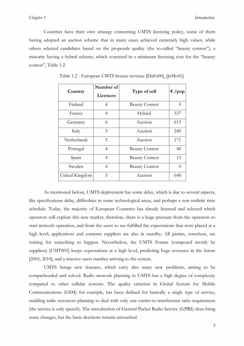
Countries have their own strategy concerning UMTS licensing policy, some of them
having adopted an auction scheme that in many cases achieved extremely high values, while
others selected candidates based on the proposals quality (the so-called “beauty contest”), a
minority having a hybrid scheme, which consisted in a minimum licensing cost for the “beauty
contest”, Table 1.2.
Table 1.2 - European UMTS licence revenue [DaEr00], [JeMo01].
Country Number of
Licences Type of sell € /pop
Finland 4 Beauty Contest 0
France 4 Hybrid 337
Germany 6 Auction 613
Italy 5 Auction 240
Netherlands 5 Auction 171
Portugal 4 Beauty Contest 40
Spain 4 Beauty Contest 15
Sweden 4 Beauty Contest 0
United Kingdom 5 Auction 648
As mentioned before, UMTS deployment has some delay, which is due to several aspects,
like specifications delay, difficulties in some technological areas, and perhaps a non realistic time
schedule. Today, the majority of European Countries has already licensed and selected which
operators will explore this new market, therefore, there is a huge pressure from the operators to
start network operation, and from the users to see fulfilled the expectations that were placed at a
high level; applications and contents suppliers are also in standby. All parties, somehow, are
waiting for something to happen. Nevertheless, the UMTS Forum (composed mostly by
suppliers) [UMTS01] keeps expectations at a high level, predicting huge revenues in the future
[2005, 2010], and a massive users number arriving to the system.
UMTS brings new features, which carry also many new problems, aiming to be
comprehended and solved. Radio network planning in UMTS has a high degree of complexity
compared to other cellular systems. The quality criterion in Global System for Mobile
Communications (GSM) for example, has been defined for basically a single type of service,
enabling radio resources planning to deal with only one carrier-to-interference ratio requirement
(the service is only speech). The introduction of General Packet Radio Service (GPRS) does bring
some changes, but the basic decisions remain untouched.

Introduction Chapter 1
4
UMTS networks will support many types of bearer services, these services being
characterised by their own intrinsic properties, like bit rate, Bit Error Rate (BER), blocking
probability, maximum delay, etc. Naturally, these imply a more complex radio network planning.
Therefore, the characterisation of main parameters (with more impact on coverage and capacity)
in UMTS, is an important task.
From the cellular operator point of view, there is one vital issue, network planning and
optimisation, which main goals are to minimise the financial cost (minimising the number of base
stations), guaranteeing the desired quality and network capacity. There are not direct and simple
methods or algorithms capable of accomplishing these goals; therefore, solving these complex
and important problems is highly motivating. Work in these areas has already begun, for example
the STORMS project [MePi99] optimises the cellular network coverage by minimising the use of
network resources (i.e. base stations and their controllers). More recently the MOMENTUM
project [MOME01] intends to perform a study on UMTS networks and produce a powerful
simulator to estimate the capacity, coverage, and Base Station (BS) deployment, based on services
definition and usage profiles and planning scenarios. In [KNLA01], it is also presented a new
approach to UMTS radio planning; however, it is build on theoretical scenarios, becoming far
from European cities reality.
As already mentioned, UMTS planning and optimisation has a huge interest and
importance to the mobile world, and it is the main objective of this thesis. In order to accomplish
this goal, some vital steps must be accomplished, like the study of UMTS network radio air
interface, services and applications definition and characterisation, system simulation algorithm,
optimisation algorithms, traffic prediction, traffic generation, and finally how to obtain some
optimal results. One main parameter, which must be optimised, is the number of BSs in the
network, or the average BS radius.
In order to accomplish these results, a software tool, capable of providing the optimum
cell radius and antenna height for UMTS-FDD, based on major network parameters, traffic
forecast and environment, was developed in this work.
This thesis is organised in 6 chapters, including this one. In Chapter 2, some basic radio
systems aspects are described, oriented to radio networks planning, like air interface, propagation,
link budget, capacity and traffic models. Chapter 3 gives an overview of 3G systems, and presents
an approach to 3G planning strategies and cellular architectures. Chapter 4 describes the
implementation of the models presented in Chapters 2 and 3, the developed planning and
optimisation algorithm being detailed. Chapter 5 deals with simulation results, where the UMTS
Forum scenario is used, and the network sensitivity to system and scenarios parameters variation

Chapter 1 Introduction
5
is tested. In Chapter 6, final conclusions are presented and future research work lines are also
proposed.
This thesis introduces some new and innovated approaches to UMTS radio network
analysis, based on system optimisation simulations results, several answers to operator’s,
frequently asked questions being given. For example: “Which is the optimum cell radius, when n
users using multi services (circuits and packets) are connected, within a set of environmental and
system parameters?”. In order to achieve these kind of answers, three main planning issues where
simulated and optimised: propagation, traffic generation and service usage characterisation. The
planning and optimisation algorithm produces good results, using less computational effort and
time compared with other heavier simulators build in European projects, like ASILUM [Héra02],
STORMS [MePi99] and more recently the MOMENTUM project [MOME01].


Chapter 2 Radio Systems Aspects
7
2 Radio Systems Aspects
2.1 System Description
2.1.1 Operation Modes and Multiple Access
UMTS may work in two different modes, the TDD and the FDD ones [3GPP00e]
[3GPP00f], which means that channels in the UL and DL will be managed in two different ways:
• In the FDD mode, two pairs of frequency bands are used at the same time, one for UL and
the other for DL. This mode uses Wideband Code Division Multiple Access (WCDMA), the
carried services being characterised by their symmetric traffic, like voice. This mode will be
the most used, being deployed in every kind of environment, particularly in macro- and
micro-cells, which is the reason why this thesis addresses the FDD mode.
• In the TDD mode, both links (UL and DL) use the same frequency, through a scheme of
Time Division - Code Division Multiple Access (TD-CDMA) in unpaired bands, which will
be advantageous to handle services with asymmetric traffic, like Internet one. It will be used
mainly in pico-cells (indoor) or in hot-spot areas.
The frequency bands that are allocated for the FDD mode are [3GPP00b]:
• 1920 – 1980 MHz : UL
• 2110 – 2170 MHz : DL
while for the TDD mode the following are allocated [3GPP00e]:
• 1900 - 1920 MHz : UL/DL
• 2010 - 2025 MHz : UL/DL
Each Radio Frequency (RF) channel in UMTS has a 5 MHz bandwidth, for both FDD and TDD
modes, which leads to a total of 12 channels in FDD and 7 in TDD.
The key properties of WCDMA are [OjPr98]:
• Improved performance over 2G systems, including:
- improved capacity;
- improved coverage, enabling migration from a 2G deployment.
• A high degree of service flexibility, including:
- support of a wide range of services, with a bit rate up to 2 Mbps, and the possibility for
multiple parallel services in one connection;
- a fast and efficient packet-access scheme.

Radio Systems Aspects Chapter 2
8
• A high degree of operator flexibility, including:
- support of asynchronous inter-base-station operation;
- efficient support of different deployment scenarios, including Hierarchical Cell Structure
(HCS) and hot-spot scenarios;
- support of evolutionary technologies, such as adaptive antenna arrays (AAA), multi-user
detection (MUD) and DL antenna diversity;
- a TDD mode designed for efficient operation in uncoordinated environments.
The wide bandwidth of WCDMA gives an inherent performance gain over previous
cellular systems, since it reduces the fading of the radio signal. In addition, WCDMA uses
coherent demodulation in UL, a feature that was not previously implemented in cellular CDMA
systems. Fast power control in DL will also increase network performance, especially in indoor
and low-speed outdoor environments, which will increase cell capacity by at least a factor of two.
Fast power control has a major impact on the performance of a WCDMA system in several ways:
• The fast fading channel may be counterbalanced by power control, changing the fading
channel into a non fading one;
• The fading channel compensation by power control leads to peaks in Mobile Station (MS)
transmission power, which affect the inter-cell interference in the network;
• Fast power control stabilises the MS power at the BS, avoiding the near-far effect in UL.
The power control algorithm is implemented based on the Signal-to-Interference Ratio
(SIR). The objective of the algorithm is to keep SIR at a suitable level by adjusting the
transmission power. The principle is very simple: the received SIR level is compared to an
appropriate threshold; if it is higher than the threshold, the receiver sends to the transmitter a
"power down" command, otherwise a "power up" command is sent.
The coverage demonstrated for WCDMA shows that it is possible to reuse GSM1800 cell
sites when migrating from GSM to UMTS, supporting high-rate services. Assumptions for this
comparison are that the average MS output power is equal in UMTS and GSM [OjPr98]. Some
simulations show that speech over WCDMA will tolerate a few dB higher path loss than GSM.
This means that WCDMA gives better speech coverage than GSM, reusing the same cell sites,
when the latter is deployed in the nearby frequency band.
One of the most important characteristics of WCDMA is the fact that power is the
common shared resource among users. In DL, the total transmitted power of an RF carrier is
shared among users, while in UL, there is a maximum tolerable interference level at the BS
receiver; this maximum interference power is shared among transmitting MSs in the cell, in the
sense that each one contributes to the interference. Power being the common resource makes
WCDMA very flexible in handling mixed services, as well as services with variable bit-rate

Chapter 2 Radio Systems Aspects
demands. Radio resource management is done by allocating power to each user (connection) to
ensure that the maximum interference is not exceeded. Reallocation of codes or time slots is
normally not needed as the bit rate demand changes, which means that the physical channel
allocation remains unchanged even if the bit rate changes. Furthermore, WCDMA requires no
frequency planning, since a cell reuse factor of one is applied.
2.1.2 WCDMA Air Interface
A unique code sequence, called "spreading code", is assigned to each user, which is used
to encode the information-bearing signal. The receiver, knowing the code sequence of the user,
decodes the received signal after reception, and recovers the original data; this is possible due to
the low cross correlations between the code of the desired user and the codes of the other users.
The bandwidth of the code signal is chosen to be much larger than the bandwidth of the
information-bearing signal, hence, the encoding process spreads the spectrum of the signal.
Therefore, a spread-spectrum technique must carry out two criteria:
1. The transmission bandwidth must be much larger than the information bandwidth;
2. The bandwidth must be statistically independent of the information signal.
The flexibility supported by WCDMA is achieved with the use of Orthogonal Variable
Spreading Factor (OVSF) codes for channelisation of different users. OVSF codes have the
characteristic of maintaining DL transmit orthogonality among users (or different services
allocated to one user) in an ideal scenario, even if they operate at different bit rates. Therefore,
one physical resource can carry multiple services with variable bit rates. As the bit rate demand
changes, the power allocated to this physical resource is adjusted, so that Quality of Service (QoS)
is guaranteed at any instant of the connection.
The ratio of the transmitted bandwidth, Bt, to information bandwidth, Bi, is called the
processing gain, Gp:
i
tp B
BG = (2.1)
Many times, the processing gain is also expressed in terms of the information bit rate, , and
the code chip rate ,
bR
cR
b
cp R
RG = (2.2)
Transport channels are the services offered by layer 1 to higher layers. Transport channels
are always unidirectional, and are defined by how and with what characteristics data is transferred
over the air interface. The classification of transport channels is the following [3GPP00g]: 9

Radio Systems Aspects Chapter 2
10
• Dedicated channels (allocated to a specific user), using inherent addressing of User Equipment
(UE). There is only one type of dedicated transport channel, the Dedicated Channel (DCH),
which can be either DL or UL. The DCH is transmitted over the entire cell, or over only a
part of it.
• Common channels (shared among several users), using explicit addressing of UE if addressing
is needed. There are six types of common transport channels:
- Broadcast Channel (BCH), which is a DL channel that is use to broadcast system and cell-
specific control information;
- Forward Access Channel (FACH), which is a DL transport channel used to carry control
information and short user packets to a MS, when its location is known to the system;
- Paging Channel (PCH), which is a DL channel used to carry control information to a MS,
when its location is not known to the system;
- Random Access Channel (RACH), which is a UL channel used to carry control information
and short user packets;
- Common Packet Channel (CPCH), which is a UL channel associated with a dedicated
channel on the DL that provides power control and control commands;
- Downlink Shared Channel (DSCH), which is a DL channel shared by several users, being
associated to one or several DL DCHs.
Physical channels usually consist of a structured layer of radio frames and time slots,
although this is not true for all physical channels. Depending on the channel bit rate of the
physical channel, the configuration of the slot varies. A radio frame, 10 ms long is a processing
unit that consists of 15 slots, its length corresponding to 38 400 chips: a slot is a unit that consists
of fields containing bits, its length corresponding to 2 560 chips. The number of bits per slot may
be different for different physical channels, and may, in some cases, vary in time.
The UL Dedicated Physical Control Channel (DPCCH) is used to carry control
information generated at layer 1, which consists of known pilot bits that support channel
estimation for coherent detection, Transmit Power-Control (TPC) commands, Feedback
Information (FBI), and an optional Transport-Format Combination Indicator (TFCI). TFCI
informs the receiver about the instantaneous transport format combination of the transport
channels mapped on the simultaneously transmitted UL Dedicated Physical Data Channel
(DPDCH) radio frame. There is one and only one UL DPCCH on each radio link. Figure 2.1
shows the frame structure of UL dedicated physical channels.

Chapter 2 Radio Systems Aspects
Pilot Npilot bits
TPC NTPC bits
DataNdata bits
Slot #0 Slot #1 Slot #i Slot #14
Tslot = 2560 chips, 10 bits
1 radio frame: Tf = 10 ms
DPDCH
DPCCHFBI
NFBI bitsTFCI
NTFCI bits
Tslot = 2560 chips, Ndata = 10*2k bits (k=0..6)
Figure 2.1 - Frame structure for UL DPDCH/DPCCH (extracted from [3GPP00c]).
In UL, a specific code is assigned to each MS for spreading purposes, which is called
scrambling code. Different channels from the same MS are distinguished by a second spreading
code, the channelisation code [3GPP00d]. The Spreading Factor (SF) and the total number of
bits per DL Dedicated Physical Channel (DPCH) slot are determined by k = 0…7, where
SF=512/2k; thus, the SF may range from 4 to 512. There is only one type of DL DPCH, within
each dedicated data generated at layer 2, and above it is transmitted in time-multiplex with control
information generated at layer 1 (known pilot bits, TPC commands, and an optional TFCI).
Hence, the DL DPCH can be seen as a time multiplex of a DL DPDCH and a DL DPCCH.
Figure 2.2 shows the frame structure of the DL DPCH.
One radio frame, Tf = 10 ms
TPC NTPC bits
Slot #0 Slot #1 Slot #i Slot #14
Tslot = 2560 chips, 10*2k bits (k=0..7)
Data2Ndata2 bits
DPDCHTFCI
NTFCI bitsPilot
Npilot bitsData1
Ndata1 bits
DPDCH DPCCH DPCCH
Figure 2.2 - Frame structure for DL DPCH (extracted from [3GPP00c]).
In UMTS the spreading operation of physical channels is carried out in two consecutive
steps:
1. Data is multiplied by the channel code (direct sequence);
11
Radio Systems Aspects Chapter 2
2. The complex signal obtained by adding several spread physical channels from I (in phase) and
Q (in quadrature) branches is multiplied by a complex value, corresponding to a transmitter
specific scrambling code.
2.1.3 Code Generation
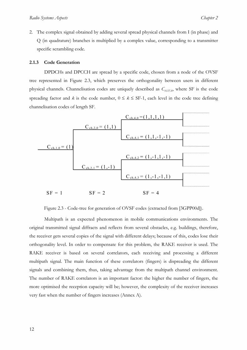
DPDCHs and DPCCH are spread by a specific code, chosen from a node of the OVSF
tree represented in Figure 2.3, which preserves the orthogonality between users in different
physical channels. Channelisation codes are uniquely described as Cch,SF,k, where SF is the code
spreading factor and k is the code number, 0 ≤ k ≤ SF-1, each level in the code tree defining
channelisation codes of length SF.
SF = 1 SF = 2 SF = 4
C ch,1,0 = (1)
C ch,2 ,0 = (1 ,1)
C ch,2 ,1 = (1 ,-1)
C ch,4 ,0 = (1 ,1 ,1 ,1)
C ch,4 ,1 = (1 ,1 ,-1 ,-1)
C ch,4 ,2 = (1 ,-1 ,1 ,-1)
C ch,4 ,3 = (1 ,-1 ,-1 ,1)
Figure 2.3 - Code-tree for generation of OVSF codes (extracted from [3GPP00d]).
Multipath is an expected phenomenon in mobile communications environments. The
original transmitted signal diffracts and reflects from several obstacles, e.g. buildings, therefore,
the receiver gets several copies of the signal with different delays; because of this, codes lose their
orthogonality level. In order to compensate for this problem, the RAKE receiver is used. The
RAKE receiver is based on several correlators, each receiving and processing a different
multipath signal. The main function of these correlators (fingers) is dispreading the different
signals and combining them, thus, taking advantage from the multipath channel environment.
The number of RAKE correlators is an important factor: the higher the number of fingers, the
more optimised the reception capacity will be; however, the complexity of the receiver increases
very fast when the number of fingers increases (Annex A).
12

Chapter 2 Radio Systems Aspects
2.1.4 Handover
Handover is one of the most important mechanisms in all wireless networks, since it
provides the maintenance of seamless communication when the MS moves from one site to
another.
In UMTS there are different types of handover mechanisms:
• Soft Handover (SH);
• Softer Handover;
• Hard Handover.
SH means that the MS is simultaneously connected to more than one Node B (BS),
Figure 2.4. The main reason for SH is the reduction of the interference into other cells, another
advantage being the performance improvement through macro diversity coming from the
diversity gain provided by the reception of one or more additional signals. In DL, the MS can
combine signals from more than one BS, since the MS sees each BS as just one more multipath
component; with this type of technique, the receiver may see different BSs as one. In the UL,
more than one BS can receive the same signal due to the reuse factor of one, combining being
done at the Radio Network Controller (RNC). The SH state is reached by a MS when the signal
strength of a neighbouring cell exceeds a certain level, but it is still below the current BS signal
strength.
R N C
N o d e B
M S
N o d e B
Figure 2.4 - Soft Handover example.
Softer Handover is the same as SH, but it works inside the same BS, which means,
handover between different sectors in a BS.
13
The Hard Handover exists because the architecture of the UMTS network will consists of
micro-cells overlaid by macro-cells, each having multiple frequency carriers, but micro- and
macro-cells may also have different ones. Hot-spot cells can have a larger number of carriers than
the surrounding ones, therefore, a different mechanism of handover is necessary between
Radio Systems Aspects Chapter 2
14
different frequencies, which is Hard Handover. The support of seamless Hard Handover through
a DL slotted mode is a key feature of WCDMA, not previously implemented in cellular CDMA.
Hard Handover is necessary for the support of HCS: a cellular system can provide very high
capacity through the micro-cell layer, offering at the same time full coverage and supporting high
mobility via the macro-cell one, therefore Hard Handover being needed to perform handover
between the different layers. A second scenario where Hard Handover is necessary is the hot-spot
one, where a certain cell that serves a high traffic area uses carriers in addition to those used by
the neighbouring cells. If the deployment of extra carriers is to be limited to the actual hot-spot
area, the possibility of Hard Handover is essential.
The Hard Handover means also that a MS makes handover between 2G systems and
UMTS, this type of handover implying a commutation between different systems, frequency
bands and air interface. Therefore, the complexity of the terminal increases, due to terminal
multi-mode and multi-band features.
2.2 Services, Applications and Scenarios
In GSM, basically one has only one major service, speech (circuit switching), from which
a network cannot offer many services and applications to a demanding user. UMTS will be able
to supply a wide range of services with different bit rates and flexible traffic asymmetry.
The services definitions are based on market forecasts by the UMTS Forum, Table 2.1.
The Speech (S) service corresponds to a GSM speech CODEC. The channel coding gives rise to
an overhead of 1.75 times the user net bit rate of the CODEC. Speech is a symmetric service
with the same amount of information in the UL as in the DL, and an occupancy factor of 0.5 is
assumed, which implies that the system should be able to handle the discontinuous transmission
mode. The Simple Messaging (SM) service is the evolution of the GSM Short Message Service
(SMS). The user net bit rate of the SM service is based on the assumption that the typical size of a
message is 40 kbyte, and an acceptable delay for this service is assumed to be 30 s (user net bit
rate 10.67 kbps). The final user net bit rate is deducted by dividing the obtained relation between
the file size and the acceptable delay to get an equivalent continuous user net bit rate. Further on,
an assumption is made of a packet efficiency factor of 0.75. The Switched Data (SD) is a 14.4
kbps CS service type similar to existing data services GSM. The same type of calculations is made
in order to find the user net bit rate for the medium and high MultiMedia (MM) services; the
services are similar to evolved World Wide Web (WWW) types of services. The typical amount of
data that needs to be transmitted for the medium MM service is 0.5 Mbytes during 14 s (user net
bit rate 286 kbps), while the same figures for the high MM service are 10 Mbytes and 53 s (user

Chapter 2 Radio Systems Aspects
15
net bit rate 1.51 Mbps). Further on, the MM services are assumed to be asymmetrical, and it is
assumed that the interactive MM service is based on a 128 kbps symmetrical connection.
Table 2.1 - Types of Services (extracted from [Garcia00]).
Services Applications
Speech
(S)
(symmetric)
• Simple one to one and one to many voice (teleconferencing) services
• Voicemail
Simple Messaging
(SM)
(asymmetric)
• SMS (short message delivery) and paging • Email delivery • Broadcast and public information messaging • Ordering/payment (for simple electronic commerce)
Switched Data
(SD)
(symmetric)
• Low speed dial-up LAN access • Internet/Intranet access • Fax Legacy services, mainly using radio modems such as PCMCIA cards, are not expected to be very significant by 2005.
Medium Multimedia
(MMM)
(asymmetric)
Asymmetric services which tend to be ‘bursty’ in nature, require moderate data rates, and are characterised by a typical file size of 0.5 Mbytes, with a tolerance to a range of delays. They are classed as PS services. • LAN and Intranet/Internet access • Application sharing (collaborative working) • Interactive games • Lottery and betting services • Sophisticated broadcast and public information messaging • Simple online shopping and banking (electronic commerce)
services
High Multimedia
(HMM)
(asymmetric)
Asymmetric services, which also tend to be ‘bursty’ in nature, require high bit rates. These are characterised by a typical file size of 10 Mbytes, with a tolerance to a range of delays. They are classed as PS services. • Fast LAN and Intranet/Internet access • Video clips on demand • Audio clips on demand • Online shopping
High Interactive
Multimedia
(HIMM)
(symmetric)
Symmetric services which require reasonably continuous and high-speed data rates with a minimum of delay. • Video telephony and video conferencing • Collaborative working and telepresence
The signalling overhead, training sequence and for the radio interference for all types of
service is 20 %. The above figures indicate representative delays that might be acceptable for PS

Radio Systems Aspects Chapter 2
16
services. In reality, a range of delay constraints will be appropriate, depending on the nature of
the application being supported over the radio interface. The delays represent a user net bit rate
that is slightly lower than the nominal rate. However, the assumption made in the calculations is
that the traffic carried for PS applications will include session control overheads (not to be
confused with the air-interface signalling overheads), including set-up and clear-down control
messages. These overheads will be invisible to the user, but will occupy the channel apparent
delay time. In the absence of detailed applications information, it is assumed that the gross traffic
bit rate offered to the air interface is equal to the nominal user bit-rate. Therefore, nominal bit
rates are used in the spectrum calculations.
Table 2.2 - Service Characteristics (adapted from [UMTS98b]).
Services User nominal bit rate [kbps]
Effective call
duration [s]
User net bit rate
[kbps]
Coding factor
Asymmetry factor
Switch Mode
Service bandwidth
[kbps] HIMM 128 144 128 2 1/1 CS 256/256 HMM 2000 53 1509 2 0.005/1 PS 15/3200 MMM 384 14 286 2 0.026/1 PS 15/572
SD 14 156 14.4 3 1/1 CS 43/43 SM 14 30 10.67 2 1/1 PS 22/22 S 16 60 16 1.75 1/1 CS 28/28
Table 2.2 shows UMTS service characteristics [UMTS98b], where one can find some
major service parameters that make possible traffic and capacity estimations, and can be explain
as follows [Garcia00]:
• User Nominal Bit Rate corresponds to the output bit rate from the source without error
protection.
• Effective Call Duration of a service corresponds to how long, on average, the service is
connected. It is based on the average call duration multiplied by the occupancy factor (see
Table 2.3). The usage of the occupancy factor (the occupancy indicates if and how much, on
average, the activity of the service will vary) implies that the system should be able to handle
the discontinuous transmission mode.
• User Net Bit Rate is a measure of the bit rate taking into account the packet efficiency factor,
which is based on considerations of practical packet networks and includes the effect of
retransmission of unsuccessful packets.
• Coding Factor is a generalised measure of the degree of coding required to transport the
service to the required quality.
• Asymmetry Factor is used to show that some services will have a different load (bit rate and
bandwidth) in the UL and DL.

Chapter 2 Radio Systems Aspects
• Service Bandwidth is the product of user nominal bit rate, coding factor and asymmetry
factor.
• Switch Mode defines if the service is CS or PS, since the call duration and the occupancy are
not suitable to characterise PS services, an estimation of effective call duration is generated.
The various service classes have different characteristics. HIMM, e.g., video telephony,
require isochronous transmission, as well as SD and S. Therefore, they are calculated as CS
services. This means that the average call duration time corresponds to the actual connection set-
up time, and that the effective call duration depends on the occupancy factor, which is 0.5 for
speech and 0.8 for video telephony. For PS services, the call duration is calculated as the sum of
time intervals, where data is actually transferred via the air interface; thus, the occupancy factor in
this scenario is equal to one, Figure 2.5. The effective call duration per service according to
occupancy and average call duration is given in Table 2.3.
Figure 2.5 - Packet transmission over the UMTS Air Interface (extracted from [UMTS98a]).
Table 2.3 - Effective Call Duration (extracted from [UMTS98b]).
Services Occupancy Average call duration [s] Effective call duration[s]HIMM 0.8 180 144 HMM 1 53.3 53.3 MMM 1 13.9 13.9
SD 1 156 156 SM 1 30 30 S 0.5 120 60
The call duration and the occupancy are not suitable to characterise packet switched
services. However, an estimation of effective call duration, and the equivalent offered bit quantity
that packet services will generate, can be based on calculations that consider busy hour calls and
an acceptable throughput and delay for packet services. The effective call duration for packet
based services should be interpreted with an acceptable delay.
17

Radio Systems Aspects Chapter 2
18
The 3GPP services classification is shown in Table 2.4, where one may find four main
traffic or service classes: Conversational, Streaming, Interactive and Background. These classes
may be described as follows [HoTo00]:
• Conversational: Real time applications (speech services, voice over IP, video telephony), strict
low end-to-end delay.
• Streaming: Streaming data transferring applications (web broadcast, video streaming on
demand), with high symmetric traffic.
• Interactive: Client-Server applications (web browsing, database access, games, tele-machines),
low round trip delay is required.
• Background: Long delay applications (SMS, e-mail, downloading databases, etc).
Table 2.4 - 3GPP traffic classes classification.
Traffic class
Conversational Streaming Interactive BackgroundConnection delay (main attribute)
Minimum fixed
Minimum variable
Moderate variable
Big variable
Buffering No Allowed Allowed Allowed
Nature of traffic Symmetric Asymmetric Asymmetric Asymmetric
Fund
amen
tal c
hara
cter
istics
Bandwidth Guaranteed bit rate
Guaranteed bit rate
No guaranteed
bit rate
No guaranteed
bit rate
Traffic is a major parameter, because radio network planning is designed as a function of
it, therefore, it is necessary to perform some traffic forecast based on users and services statistics.
Table 2.5 shows statistical information that is fundamental for the network planning process,
since most of traffic estimation is dependent on user density, therefore, the corresponding
network capacity estimation for each operational environment may be obtained. Only three of the
operational environments (marked in bold in Table 2.5) contribute to the maximum total amount
of capacity required, because they coexist in the same geographical area, and, of course, present
high user density values.
It should be noted that the conclusions made here are dependent upon market forecasts
data for the years up to 2005 [UMTS98b]. For example, it is assumed that 90% of the total
speech and low speed data traffic will be carried over existing 2G networks within this period. It
is also considered that 60% of the indoor traffic will be carried over license-exempt networks,
and that high (2 Mbps) and medium (384 kbps) multimedia services are PS, which are tolerant to

Chapter 2 Radio Systems Aspects
19
delay. It is important to note that although the majority of users will continue to use speech, most
of the capacity is needed for multimedia services. The UMTS Forum (Spectrum Aspects Group)
assumptions are that market is expected to continue to grow strongly after this date, and
additional spectrum will be required in the future (up to year 2010).
Table 2.5 - Operational environment and cell types (extracted from [UMTS98b]).
Operational environments Density of potential users/km2 Cell Type CBD/Urban(in building) 180 000 Micro/pico
Suburban (in building or on street) 7 200 Macro Home (in building) 380 Pico Urban (pedestrian) 108 000 Macro/micro Urban (vehicular) 2 780 Macro/micro
Rural in- & out-door 36 Macro
UMTS is primarily envisaged for multi-service in these environments, and
inhomogeneous traffic distributions are expected to occur, where the asymmetric traffic will be
the main reason for this.
2.3 Propagation
2.3.1 Propagation Models
In order to perform radio network planning, among other things, it is essential to
estimate the propagation loss as a function of a given propagation environment (indoor, outdoor,
urban, rural, etc). This key parameter makes the estimation of several other main network
planning parameters possible, like average mobile received power, cell coverage, interference and
load factor.
In this thesis, several propagation models were studied, but only the following are
presented, due to their particular characteristics:
• 3GPP;
• COST 231 - Walfisch-Ikegami;
• COST 231 - Hata.
3GPP proposes a propagation model for macro- and micro-cells [3GPP00a], where two
propagation environments are considered. For each environment, a different formulation is used
to evaluate the path loss. An important parameter to be defined is the Minimum Coupling Loss
(MCL), i.e., the minimum distance loss, including antenna gain, measured between antenna
connectors; the following values are assumed for MCL: 70 dB for the macro-cellular

Radio Systems Aspects Chapter 2
20
environment, and 53 dB for the micro-cellular one. The MCL is most important for the study of
the near-far effect limitations.
The macro-cell model is applicable for scenarios in urban and suburban areas outside the
high rise core, where buildings are of nearly uniform height [ETSI98]. Also the micro-cell model
is adopted from [ETSI98]. This model is to be used for spectrum efficiency evaluations in urban
environments, through a Manhattan-like structure, in order to properly evaluate the performance
in micro-cell situations that will be common in European cities at the time of UMTS deployment.
The proposed model is a recursive one, which calculates the path loss as a sum of Line of Sight
(LoS) and Non Line of Sight (NLoS) segments. The shortest path along streets between the BS
and the MS has to be found within the Manhattan environment (for more details see Annex B).
The well-know semi-empirical Walfisch and Bertoni [WaBe88] and Ikegami [IkYU84]
propagation models, were adapted by COST 231 based on measurements performed in Europe
[DaCo99], producing acceptable estimations for urban environments. Like any kind of
propagation model, this one also has some constrains, e.g., on frequency band, BS height and
distance. For example, the validity range of this model in frequency is [800, 2000] MHz, while
UMTS works in [1900, 2170] MHz, hence, for the upper band of UMTS one will be using the
model outside its range; nevertheless, this does not imply a large error, since the difference in
frequency is not large. This model has also distance limitations between BS and MS, being
applicable for NLoS in [0.2, 5] km, and in [0.02, 0.2] km for LoS. These ranges satisfy the major
UMTS micro-cell radius, mainly in urban areas. Therefore, this model may be used for estimation
of signal propagation loss in UMTS (more details in Annex B).
The Okumura-Hata Model empirical propagation model is based on approximations
performed by Hata [Hata80] supported on Okumura et al. model [OOKF68]. It gives the
average field intensity, which depends on frequency, distance, antennas height, type of
environment where the MS moves, and characteristics between the BS and MS. This model is
applicable to long distances between the MS and the BS. COST 231 has investigated this model,
and created a new one, called the COST 231-Hata-Model [DaCo99], which corresponds to
extending Hata's model to the frequency band [1500, 2000] MHz (more details in Annex B).
Combining the output of one of these models (Path Loss) with the link budget, it is
possible to estimate the cell coverage as a function of a given service; therefore, it is possible to
estimate the number of cells in a given area, which is one major goal of this work.
These models have some validity limitations, as for example frequency up to 2000 MHz;
as explained before this, does not imply a large error. In order to choose a model to be
implemented in this thesis, some differences among these models must be identified, like
propagation environments or cell types (dimensions); the 3GPP model is more dedicated to

Chapter 2 Radio Systems Aspects
micro-cells in a city with a Manhattan like urban structure; the COST 231 – Hata is for macro-
cells and urban and suburban environments; the COST 231-Walfisch-Ikegami model is dedicated
to dense urban (European type) scenarios and for micro-cells. In this work, the main goal is to
achieve optimal network values for this last scenario, therefore, the COST 231-Walfisch-Ikegami
propagation model was selected and implemented in this thesis.
2.3.2 Link Budget
In order to perform radio network planning, one needs to establish the link budget for
coverage, capacity and optimisation reasons. Reference [HaTo00] presents the link budget
algorithm, which enables the estimation of the allowed maximum propagation loss LPmax.
A common parameter between propagation models and link budget algorithms is the path
loss, LP,
[ ] [ ] [ ] [ ] [ ] [ ] [ ] [ ]dBdBdBmdBdBidBidBmdB ∑∑ −−−+++= MxSminSHrttpmax FLRGGGPL (2.3)
where:
• LPmax is the maximum propagation loss allowed for a given service;
• Pt is the transmitted power (delivered to the antenna);
• PTx is the transmitter output power;
• Pr is the antenna received power;
• PRx is the receiver input power;
• Gt is the maximum transmitter antenna gain;
• Gr is the maximum receiver antenna gain;
• GSH is the soft handover gain;
• RSmin is the receiver sensitivity for a given service bearer;
• Lx represents additional attenuations in a link, which may be user body loss LUB, cable loss LC,
and others (car loss) LOther.
• FM represents fading margins, i.e., fast fading margin FFM, and slow fading margin FSM.
The Equivalent Isotropic Radiated Power (EIRP), depends on Pt and Gt as follows:
[ ] [ ] [dBidBmdBm tt GPEIRP += ]
]
(2.4)
where Pt is defined by:
[ ] [ ] [dBdBmdBm CTxt LPP −= ] (2.5)
and PRx, is defined as follows:
[ ] [ ] [dBdBmdBm CrRx LPP −= (2.6)
21

Radio Systems Aspects Chapter 2
A major parameter in radio network planning is RSmin, because it depends on the service
type (energy of bit over noise and bit rate), therefore, different LPmax and cell radius are expected
for each service. RSmin, is defined as follows:
[ ][ ]
[ ] [dBmdBdB
dBm NGNE
R P0
bSmin +−= ] (2.7)
where:
• Eb/N0 is a relation between energy of bit and noise density which depends of the service,
mobile speed, receiver algorithms and BS antenna structure;
• GP is the processing gain, which depends on the relation between chip rate and bit rate (2.2);
• N is the total effective noise plus interference power.
N can be written as:
[ ][ ] [ ] )1010log(10 10/10/
dBmdBmdBm IN RRN += (2.8)
where the receiver interference power RI , is given by:
[ ][ ] [ ]( ) [ ] )1010log(10 10/10/
dBmdBmdBdBm NmN RIR
IR −= + (2.9)
and the receiver noise power RN , is given by:
[ ] [ ] [ ][ ]cps6
dBm/HzdBm 10840.3log10 ⋅+= NON RR (2.10)
where:
• Im is the interference margin;
• RNO is the receiver noise density;
The receiver noise density, RNO depends on the thermal noise density No and on the noise factor,
FN.
[ ] [ ] [dBdBm/HzdBm/Hz NoNO FNR ]+= (2.11)
Using propagation models and link budgets algorithms, it is possible to estimate the
interference load in a given area, therefore in a given cell (BS).
To estimate the amount of supported traffic (capacity) per BS, it is very important to
calculate the interference, because cellular systems that use a frequency reuse factor of 1 are
typically strongly interference-limited by the air interface. Therefore, the amount of interference
and cell capacity must be estimated.
22
Chapter 2 Radio Systems Aspects
2.4 Capacity and Interference
Capacity evolution is a key issue in cellular systems, it being important to estimate the
number of users per cell and per MHz. Capacity in UMTS depends mainly on: DL total power,
available channel codes that depend on users behaviour (used services, bit rate, Eb/N0 targets),
quality network targets (blocking and delay), urban environment (multipath spread), signalling,
and soft handover channels.
As shown in [HaTo00], capacity depends more on the load in DL than UL. The reason is
that in DL the maximum transmission power is the same, regardless of the number of users, and
it is shared among users, while in UL each additional user has its own power amplifier. Therefore,
even with low load in DL, coverage decreases as a function of the number of users. So one may
conclude that coverage is limited by the UL, while capacity is DL limited.
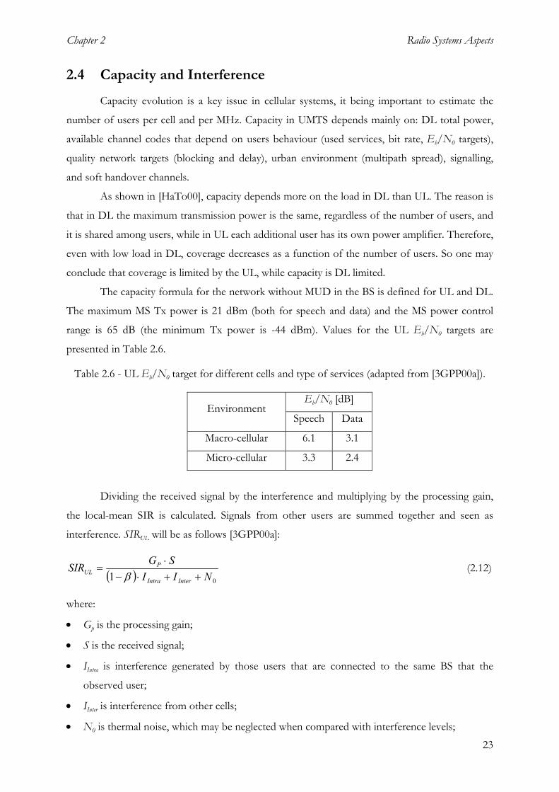
The capacity formula for the network without MUD in the BS is defined for UL and DL.
The maximum MS Tx power is 21 dBm (both for speech and data) and the MS power control
range is 65 dB (the minimum Tx power is -44 dBm). Values for the UL Eb/N0 targets are
presented in Table 2.6.
Table 2.6 - UL Eb/N0 target for different cells and type of services (adapted from [3GPP00a]).
Eb/N0 [dB] Environment
Speech Data
Macro-cellular 6.1 3.1
Micro-cellular 3.3 2.4
Dividing the received signal by the interference and multiplying by the processing gain,
the local-mean SIR is calculated. Signals from other users are summed together and seen as
interference. SIRUL will be as follows [3GPP00a]:
( ) 01 NIISGSIR
InterIntra
PUL ++⋅−
⋅=
β (2.12)
where:
• Gp is the processing gain;
• S is the received signal;
• IIntra is interference generated by those users that are connected to the same BS that the
observed user;
• IInter is interference from other cells;
• N0 is thermal noise, which may be neglected when compared with interference levels;
23
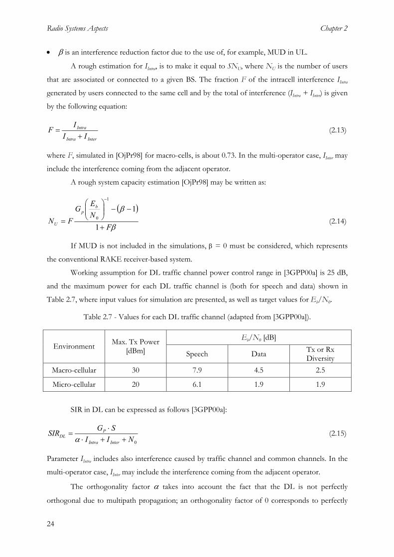
Radio Systems Aspects Chapter 2
• β is an interference reduction factor due to the use of, for example, MUD in UL.
A rough estimation for IIntra, is to make it equal to SNU, where NU is the number of users
that are associated or connected to a given BS. The fraction F of the intracell interference IIntra
generated by users connected to the same cell and by the total of interference (IIntra + IInter) is given
by the following equation:
InterIntra
Intra
III
F+
= (2.13)
where F, simulated in [OjPr98] for macro-cells, is about 0.73. In the multi-operator case, IInter may
include the interference coming from the adjacent operator.
A rough system capacity estimation [OjPr98] may be written as:
( )
β
β
FNE
GFN
bp
U +
−−
=
−
1
11
0 (2.14)
If MUD is not included in the simulations, β = 0 must be considered, which represents
the conventional RAKE receiver-based system.
Working assumption for DL traffic channel power control range in [3GPP00a] is 25 dB,
and the maximum power for each DL traffic channel is (both for speech and data) shown in
Table 2.7, where input values for simulation are presented, as well as target values for Eb/N0.
Table 2.7 - Values for each DL traffic channel (adapted from [3GPP00a]).
Eb/N0 [dB] Environment Max. Tx Power
[dBm] Speech Data Tx or Rx Diversity
Macro-cellular 30 7.9 4.5 2.5
Micro-cellular 20 6.1 1.9 1.9
SIR in DL can be expressed as follows [3GPP00a]:
0NIISG
SIRInterIntra
PDL ++⋅
⋅=
α (2.15)
Parameter IIntra includes also interference caused by traffic channel and common channels. In the
multi-operator case, IInter may include the interference coming from the adjacent operator.
The orthogonality factor α takes into account the fact that the DL is not perfectly
orthogonal due to multipath propagation; an orthogonality factor of 0 corresponds to perfectly
24

Chapter 2 Radio Systems Aspects
orthogonal intra-cell users, while for the value of 1 intra-cell interference has the same effect as
inter-cell one.
Table 2.8 presents values assumed for the orthogonality factor α and for maximum
transmitting power in 3GPP simulations.
Table 2.8 - Simulation input values (adapted from [3GPP00a]).
Environment Orthogonality factor α Total max. BS Tx Power [dBm]
Macrocellular 0.4 43
Microcellular 0.06 33
Compared to a micro-cellular environment, a signal in macro-cellular one follows a more
complex path, which is translated into a more complex multipath; because of these higher
distances (more reflection and refraction points), the α factor in a macro-cellular environment is
expected to be higher than in a micro-cellular one.
2.5 Traffic Models
In 2G cellular networks like GSM, where voice (in CS) is the only service being supported
(or almost), traffic has some well-know characteristics, like symmetry in UL and DL, channel
assignment, call arrival rate, call duration model and blocking behaviour. This type of traffic is
very easy to simulate or predict by an analytical expression, the well-know Erlang B model
[Rapp96]:
∑=
=C
i
i
c
iA
CA
B
0 !
! (2.16)
where B is the blocking probability, A is the offered traffic in Erlang, and C is the number of
channels. One should note that in UMTS the number of channels is not deterministic, so this
model cannot be used, unless very crude estimations are intended.
PS in relation to CS has some additional complexity, namely traffic asymmetry between
UL and DL, bursty traffic, and packet delay behaviour. A service like Internet is a very popular
PS example, which shows how different it can be.
In order to simulate the mixed CS and PS services behaviour, a study on traffic models
was performed, aiming to build a traffic generator, traffic properties were identified. Connections
arrival rate can be characterised by a Poisson distribution [Yaco93]:
25
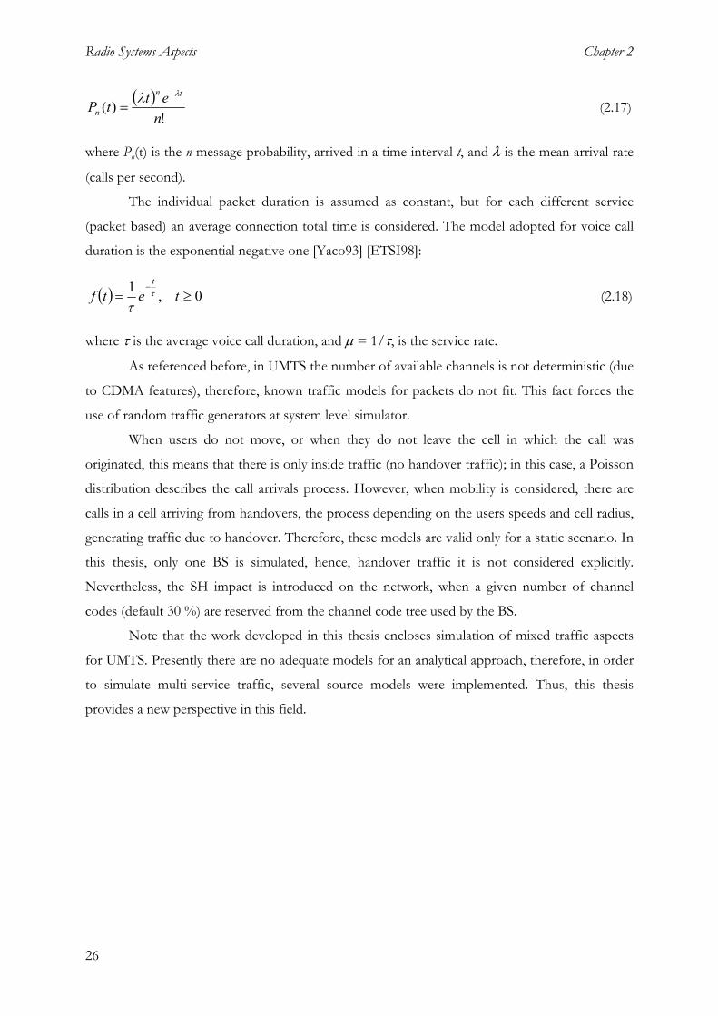
Radio Systems Aspects Chapter 2
( )!
)(n
ettPtn
n
λλ −
= (2.17)
where Pn(t) is the n message probability, arrived in a time interval t, and λ is the mean arrival rate
(calls per second).
The individual packet duration is assumed as constant, but for each different service
(packet based) an average connection total time is considered. The model adopted for voice call
duration is the exponential negative one [Yaco93] [ETSI98]:
( ) 0,1≥=
−tetf
tτ
τ (2.18)
where τ is the average voice call duration, and µ = 1/τ, is the service rate.
As referenced before, in UMTS the number of available channels is not deterministic (due
to CDMA features), therefore, known traffic models for packets do not fit. This fact forces the
use of random traffic generators at system level simulator.
When users do not move, or when they do not leave the cell in which the call was
originated, this means that there is only inside traffic (no handover traffic); in this case, a Poisson
distribution describes the call arrivals process. However, when mobility is considered, there are
calls in a cell arriving from handovers, the process depending on the users speeds and cell radius,
generating traffic due to handover. Therefore, these models are valid only for a static scenario. In
this thesis, only one BS is simulated, hence, handover traffic it is not considered explicitly.
Nevertheless, the SH impact is introduced on the network, when a given number of channel
codes (default 30 %) are reserved from the channel code tree used by the BS.
Note that the work developed in this thesis encloses simulation of mixed traffic aspects
for UMTS. Presently there are no adequate models for an analytical approach, therefore, in order
to simulate multi-service traffic, several source models were implemented. Thus, this thesis
provides a new perspective in this field.
26

Chapter 3 UMTS Planning
3 UMTS Planning
3.1 Cellular Structure
Typically, the cellular structure of GSM is deployed as a function of traffic, therefore,
special areas where traffic demand is huge (shopping, business, entertainment centres, etc) need
special indoor coverage provided by small cells, the pico-cells. For urban outdoor scenarios,
where traffic is generated mainly by pedestrian and vehicle users, micro-cells are deployed. For
suburban and rural areas, where traffic is expected to be low, macro-cells are enough to serve the
area, but in urban areas, macro-cells are also used, for optimisation issues, like carrying fast users
or traffic management.
Naturally, scenarios for UMTS are quite the same, but there are some important
differences in the operation modes: for indoor environments (pico-cells) where the asymmetric
and high bit rates services are expected to be more used, the TDD mode will support this
services. For the majority of micro- and macro-cells, the mode of operation will be FDD.
There are several types of cells for different environments, Figure 3.1. In this work, the
satellite cell is ignored, and in many cases the pico-cell is also ignored, because this type of cell is
only used for the TDD mode.
Figure 3.1 - General Hierarchical Cell Structure.
Based on [UMTS98a], the averaged cell radius for the Central Business District (CBD) is
assumed to be 75 m, for both years 2005 and 2010. The average cell radius for the other two
operational environments of significance (the urban, pedestrian and vehicular) is about 700 m for
year 2005, and will decrease approximately to 600 m for year 2010. An average cell radius of 700
m describes an environment where the cell sizes varies from 400 m to 1 km. Similar to this, the
average cell radius of 600 m corresponds to values between 300 to 900 m, Table 3.1.
27

UMTS Planning Chapter 3
Table 3.1 - Assumed BSs radius and cell areas.
Cell Type Distance [km] Cell area [km2]
Macro 1 3.14
Micro 0.4 0.5
Pico 0.075 0.017
For macro- and micro-cells, the maximum available data rate is 384 kbps with full
mobility, while for micro- and pico-cells with low mobility the data rate goes up to 2 Mbps.
In WCDMA, the common radio resource to be used by all users in the DL is power, since
the frequency re-use of one is used for all bearer services. There is a need to plan for the number
of BSs, according to the level of traffic that is expected, including the service mixture. This can be
performed by using an automatic planning tool with the following inputs: expected services, radio
propagation models, link budget parameters, mobile speeds, traffic loads, quality requirements,
etc. However, since UMTS is not yet in operation, there is no such tool that has been assessed by
experience.
For an optimal UMTS radio network, it is proposed that UMTS will be planned by using
a hierarchical cell structure, composed of macro-, micro- and pico-cells, like in Figure 3.2. The
choice on the UMTS mode, FDD or TDD, and on the superposition of the cells, needs to be
done according to traffic demands. With a flexible deployment, it will be possible for an operator
to re-deploy pico-cell channels in some indoor locations, and use these channels again in macro-
cells in urban areas. Traffic is assigned to pico-cells in CBD scenarios that use the HMM service,
because all urban-pedestrian HMM traffic is allocated to micro-cells (partly at a lower data rate),
and all HMM urban-vehicular traffic is carried by macro-cells at a lower data rate.
FDD macrocell
TDD/FDD overlay cell
FDD microcell
(picocell)
F1
F1
F1
F2
F2
F2
F2
F2
F2
F2
f3
f3
F2
f3f1
F1/f1 : pico and macro cells
F2 : macro cell layer
f3 : micro cell layer
28

Chapter 3 UMTS Planning
Figure 3.2 - UMTS Hierarchical Cell Structure (extracted from [UMTS98a]).
The FDD macro-cell provides wide area coverage, and is also used for high-speed
mobiles. The micro-cells are used at street level for outdoor coverage, to provide extra capacity
where macro-cells could not cope. A cluster of them is shown in Figure 3.2, although they can be
deployed singly. The shape of these micro-cells will not be hexagonal, but rather canyon-like,
which reflects the topography of the streets, with a distance between 200 and 400 m; note that
this distance is specific of the city type. Pico-cells will be deployed mainly indoors, in areas where
there is a demand for high data rate services, such as laptops networking or multimedia
conferencing. The way in which these pico-cells can be deployed will depend on their maximum
range in given environments (indoor and outdoor), which will be about 75 m. A limiting factor
will be the range of mobile terminals when used for high data rate services, given the high
demand this will place on batteries and in the BS power budget.
Table 3.2 shows dimensions for sectorised cells, cell radius and sectored hexagon cell
area. The sectored hexagon cell area is calculated according to [UMTS98b]:
sec
2
sec 323
NR
A cell= (3.1)
where Rcell is the cell radius, and Nsec is the number of sectors per cell. A simplified model for the
hexagonal cell is used instead of a three-sector model. This is shown in Figure 3.3.
S2
S1
S 3 Rcell
S 1, S 2, S 3 = SectorRcell = Radius
Figure 3.3 - Simplified Sector Cells (adapted from [UMTS98b]).
Table 3.2 - Cell Dimensions per Operating Environment (adapted from UMTS98b]).
29
Cell radius [km] Sectored Hexagon Cell
Area [km2] Operational environments Sectors
per base2005 2010 2005 2010
CBD/Urban (building) 3 0.075 0.075 0.005 0.005
Suburban (building / street) 3 3 2.0 7.79 3.46
Home (building) 1 0.02 0.02 0.001 0.001
Urban (pedestrian) 3 0.7 0.6 0.424 0.312
Urban (vehicular) 3 0.7 0.6 0.424 0.312
Rural in- & out-door 3 8 8 55.43 55.43

UMTS Planning Chapter 3
Table 3.2 shows the cell radius and sector area as a function of operational environments,
based on traffic forecast for years 2005 and 2010. Note that, mainly in urban scenarios, the cell
radius decreases by the year 2010 relatively to 2005.
3.2 Other systems
3.2.1 GSM
Network planning in GSM [Yaco93] has basically two main areas, capacity and
interference, because GSM uses FDMA/TDMA as air interface access schems. Capacity is
limited by the number of available carriers in a cluster (group of cells using different frequencies)
or in a cell, while interference (mainly co-channel interference) is limited by the cell reuse
distance. Figure 3.4 represents a typical GSM cell structure, (several clusters of four cells), where
the different colours represent different frequency groups.
Figure 3.4 - GSM "classical" planning.
To increase capacity in GSM the reuse factor must be decreased, but since co-channel
interference increases, a trade-off between the reuse factor and the ratio of carrier to co-channel
interference must be achieved. Note that in GSM the thermal noise is usually neglected compared
to interference.
UMTS has major differences compared to GSM mainly at the radio interface level. The
carrier spacing in GSM is 200 kHz, while in UMTS-WCDMA is 5 MHz. The frequency reuse
factor used in GSM typically is 3 or 4, while in UMTS the reuse factor is one, due to CDMA. Due
to multipath propagation, signals suffers several delays, leading to a lack of absolute orthogonality
among receiving signals, i.e., received signals have some correlation, which means interference; in
order to minimise this critical element, WCDMA performs power control at 1500 Hz. GSM also
has power control but only at 2 Hz. In the quality control field, UMTS is also different, since
30

Chapter 3 UMTS Planning
31
radio resource management is essential (5 MHz gives multipath diversity), while in GSM the main
issue is frequency planning (frequency hopping).
Packet switching is a key element, load-based in UMTS, and time-slot based in GSM.
Finally, UMTS offers DL diversity, improving capacity.
3.2.2 CdmaOne
The IS-95/cdmaOne [OjPr98] air interface uses a carrier with 1.25 MHz of bandwidth.
The network is synchronous within a few microseconds. This characteristic allows the use of long
codes sequence, with different phase offsets as pilot sequences. However, to obtain synchronism
a system like Global Positioning System (GPS) is required. Such characteristics are not applicable
to UMTS.
The used chip rate in CdmaOne is 1.2288 Mcps. Table 3.3 shows the main parameters
that characterise cdmaOne compared with UMTS.
Table 3.3 - cdmaOne Air Interface (extracted from [OjPr98]).
Characteristics CdmaOne UMTS-FDD
Bandwidth [MHz] 1.25 5
Chip Rate [Mcps] 1.2288 3.84
Frequency band [MHz]
Frequency band [MHz]
869 – 894 (800 band)
1930 – 1990 (1900 band)
UL 1920 - 1980
DL 2110 - 2170
Soft Handover Yes Yes
Power Control
UL : Open loop + fast closed
loop (800 Hz)
DL : Slow quality loop
1500 Hz, both UL and DL
In IS-95/cdmaOne, like in GSM, coverage is limited by only one service, speech.
Deployment of BSs is therefore an easy task, because with a reuse factor of one network planning
"it is just planting base stations". Therefore, the radio network planning of IS-95/cdmaOne is just
to follow a simple hexagonal structure (with a reuse factor of one) and to make a suitable
distribution of codes by several BSs.

UMTS Planning Chapter 3
32
3.3 Parameters for Radio Network Planning
3.3.1 Radio Network Planning Procedure
Network planning is a very complex task that needs to be constantly updated. UMTS
network planning covers two major areas, radio network planning and transport network
dimensioning:
• radio network planning deals with the calculation of link budget, capacities, and of course the
required number of cells; in addition, it includes detailed coverage and parameter planning
for individual sites;
• in transport network dimensioning, the capacities of the links between BS and RNC, the
number of RNC, switches and other network elements are calculated.
A large number of different services associated to different bit rates makes the process of
network planning for 3G systems much more complex, as compared to 2G ones. In order to
produce a good radio network planning, it is necessary to have a complete knowledge about the
radio environment. Some approximations can be made based on general radio channel
characteristics, however, since the radio environment is highly variable, even within the area of
one cell, detailed measurements and optimisation need to be performed for each individual cell.
The radio network planning progress can be divided into three phases:
• preparation;
• estimation of cell count;
• detailed network planning.
In the preparation phase, coverage and capacity objectives are established, the network
planning strategy is defined, and initial design operating parameters determined. Coverage and
capacity objectives are a trade-off between desired quality and overall network cost. A smaller
signal outage probability means smaller cells, thus, higher overall network costs; smaller
interference outage probability means smaller capacity, thus, also higher cost. A typical outage
probability target is 5 to 10%, corresponding to 90 to 95% availability/coverage probability. The
coverage probability can be different for different services as discussed below. Blocking
probability and delay quality targets must also be defined.
The estimation of cell count depends on the number of users in a given area, which is
obtained by multiplying the population in the area by penetration forecast values. The number of
users and offered traffic per user determine the overall offered traffic. When cell capacity and
area are known, a rough number of cells can be determined, as show in Figure 3.5. The user
profile forecast is calculated in the following subsection.

Chapter 3 UMTS Planning
Number of users in agiven area
Penetrationpercentage
Population in a givenarea X
XAverage Traffic perUser
User Profile Forecast
Offered Traffic Cell/km2Capacity/Cell
Cell Count
Figure 3.5 - Cell Count Forecast Algorithm.
In order to perform radio network planning, the network load factor is a vital parameter,
because power is the shared resource in UMTS radio interface. The network load estimation is
needed in order to perform the necessary changes on the network and develop an optimal
network configuration. The load factor has some differences between the DL and the UL. For
UL, the load factor is written as follows [HaTo00]:
( ) ( )∑∑==
⋅⋅
+
+=+=N
j
jjj
b
c
N
jjUL
vRNE
RiLi
1
0
1 1
111η (3.2)
where Rc is the chip rate, j is the "user", Rj is the user j bit rate, vj is the user j activity factor,
(Eb/N0)j, is the ratio of bit energy over the noise spectral density for user j, i is the ratio of other
cells to own cell interference and Lj is the load factor of one connection. In DL, the load factor,
ηDL, can be defined based on a principle similar as for the UL, although some parameters are
slightly different:
33
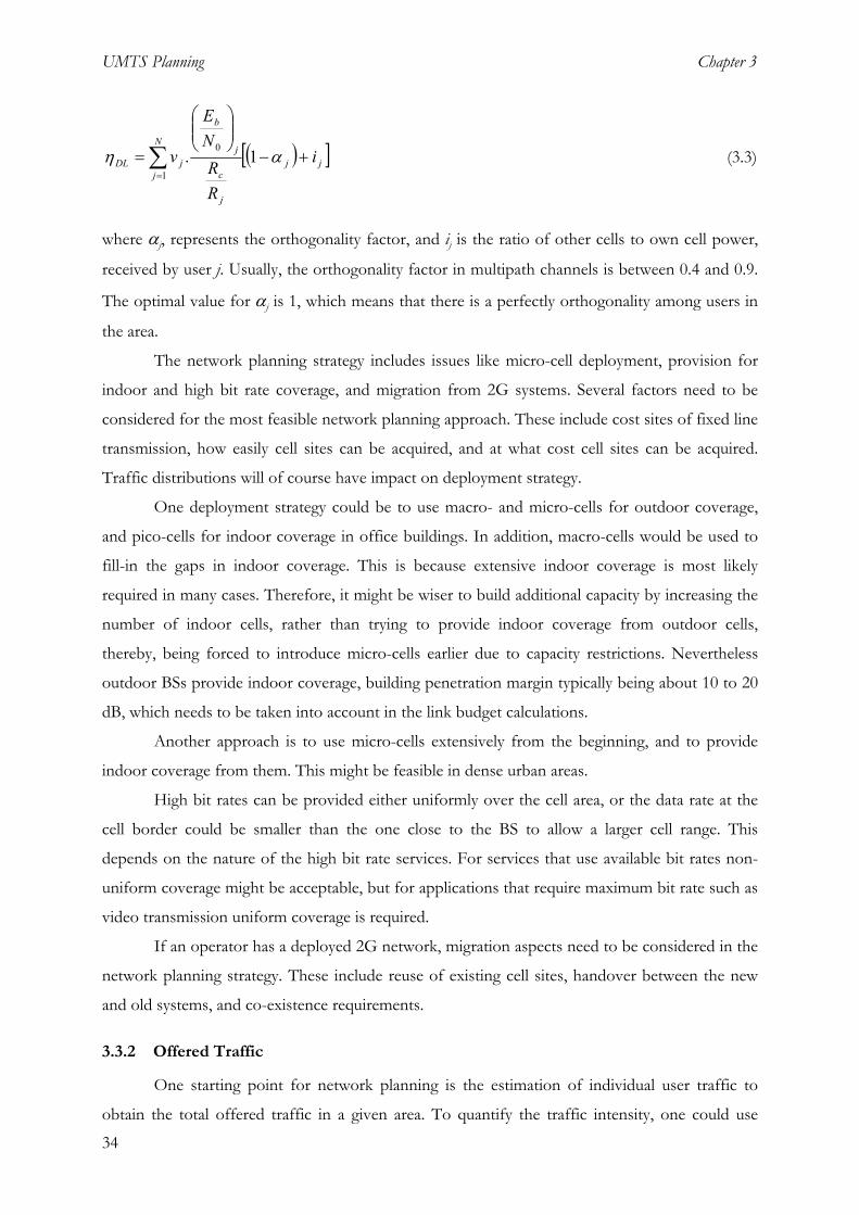
UMTS Planning Chapter 3
( )[ jj
N
j
j
c
j
b
jDL i
RR
NE
v +−
= ∑=
αη 1.1
0 ] (3.3)
where αj, represents the orthogonality factor, and ij is the ratio of other cells to own cell power,
received by user j. Usually, the orthogonality factor in multipath channels is between 0.4 and 0.9.
The optimal value for αj is 1, which means that there is a perfectly orthogonality among users in
the area.
The network planning strategy includes issues like micro-cell deployment, provision for
indoor and high bit rate coverage, and migration from 2G systems. Several factors need to be
considered for the most feasible network planning approach. These include cost sites of fixed line
transmission, how easily cell sites can be acquired, and at what cost cell sites can be acquired.
Traffic distributions will of course have impact on deployment strategy.
One deployment strategy could be to use macro- and micro-cells for outdoor coverage,
and pico-cells for indoor coverage in office buildings. In addition, macro-cells would be used to
fill-in the gaps in indoor coverage. This is because extensive indoor coverage is most likely
required in many cases. Therefore, it might be wiser to build additional capacity by increasing the
number of indoor cells, rather than trying to provide indoor coverage from outdoor cells,
thereby, being forced to introduce micro-cells earlier due to capacity restrictions. Nevertheless
outdoor BSs provide indoor coverage, building penetration margin typically being about 10 to 20
dB, which needs to be taken into account in the link budget calculations.
Another approach is to use micro-cells extensively from the beginning, and to provide
indoor coverage from them. This might be feasible in dense urban areas.
High bit rates can be provided either uniformly over the cell area, or the data rate at the
cell border could be smaller than the one close to the BS to allow a larger cell range. This
depends on the nature of the high bit rate services. For services that use available bit rates non-
uniform coverage might be acceptable, but for applications that require maximum bit rate such as
video transmission uniform coverage is required.
If an operator has a deployed 2G network, migration aspects need to be considered in the
network planning strategy. These include reuse of existing cell sites, handover between the new
and old systems, and co-existence requirements.
3.3.2 Offered Traffic
One starting point for network planning is the estimation of individual user traffic to
obtain the total offered traffic in a given area. To quantify the traffic intensity, one could use
34
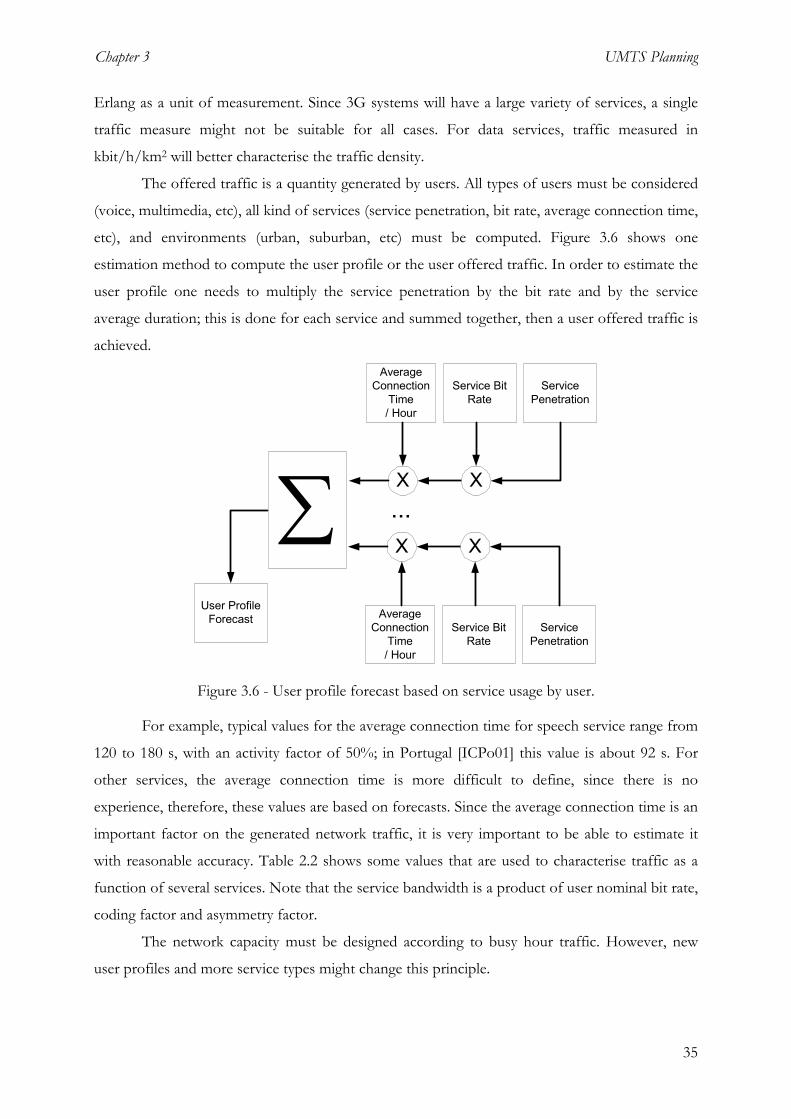
Chapter 3 UMTS Planning
Erlang as a unit of measurement. Since 3G systems will have a large variety of services, a single
traffic measure might not be suitable for all cases. For data services, traffic measured in
kbit/h/km2 will better characterise the traffic density.
The offered traffic is a quantity generated by users. All types of users must be considered
(voice, multimedia, etc), all kind of services (service penetration, bit rate, average connection time,
etc), and environments (urban, suburban, etc) must be computed. Figure 3.6 shows one
estimation method to compute the user profile or the user offered traffic. In order to estimate the
user profile one needs to multiply the service penetration by the bit rate and by the service
average duration; this is done for each service and summed together, then a user offered traffic is
achieved.
∑ ...
AverageConnection
Time/ Hour
X
Service BitRate
ServicePenetration
X
AverageConnection
Time/ Hour
X
Service BitRate
ServicePenetration
X
User ProfileForecast
Figure 3.6 - User profile forecast based on service usage by user.
For example, typical values for the average connection time for speech service range from
120 to 180 s, with an activity factor of 50%; in Portugal [ICPo01] this value is about 92 s. For
other services, the average connection time is more difficult to define, since there is no
experience, therefore, these values are based on forecasts. Since the average connection time is an
important factor on the generated network traffic, it is very important to be able to estimate it
with reasonable accuracy. Table 2.2 shows some values that are used to characterise traffic as a
function of several services. Note that the service bandwidth is a product of user nominal bit rate,
coding factor and asymmetry factor.
The network capacity must be designed according to busy hour traffic. However, new
user profiles and more service types might change this principle.
35

UMTS Planning Chapter 3
36
Figure 3.7 describes the calculation of Offered Bit Quantity (OBQ) witch is based on the
population density and penetration forecasts in the EU (15 countries). In the calculations of the
number of users that need to be served, at least the following factors should be accounted for:
• population living in a given area;
• population working in a given area;
• vehicle traffic;
• special events, and use of recreational areas.
The population density is divided into three environments: urban, suburban and rural.
The potential users per km2 are estimated for each environment. Then, the penetration rate of
users per service is multiplied with the potential number of users per km2, which gives the actual
number of users per service per km2. Users will not use the service all time, therefore, one has to
define busy hour call attempts. This means that one looks at the busiest hour of the day and
estimates the average number of calls per user in that hour. Therefore, the busy hour call attempt
is multiplied by the actual number of users per service per km2, which gives the equivalent
number of active users during the busy hour for one km2. The active users multiply the
throughput or service bandwidth in kbps during the busy hour and the effective call duration (the
duration of the call), which gives the OBQ during the busy hour. This is also explained by the
following equation:
OBQ=BusyHourCallAttempts × Penetration×(Users/km2) × ServiceBandwidth × EffectiveCallDuration (3.4)
Table 3.4 shows some forecast results in DL for the OBQ parameter.

Chapter 3 UMTS Planning
Population density EU15
Potential users / km2 per environment
Urban RuralSuburban
Penetration of users per servicefor year 2005 and 2010
Calls during busy hour per UMTS service
[pot. users / km2]
[users / km2]
[calls / hour / km2]
Service bandwith and duration
[kbit / hour / km2]
Offered Bit Quantity
[calls/hour/service/environment]
UNIT AGGREGATED UNIT
[population]
[pot. users / km2]
[penetration / km2]
[Kbit/call]
Figure 3.7 - The OBQ calculation steps (extracted from [UMTS98b]).
Table 3.4 - OBQ in DL for year 2005 (adapted from [UMTS98a]).
OBQ [kbit/h/km2] Service
CBD Urban-pedestrian Urban-vehicular
HIMM 9.56E+06 1.53E+06 2.62E+03
HMM 2.76E+08 7.86E+07 1.35E+05
MM 2.21E+07 6.42E+06 1.10E+04
SD 8.73E+06 2.62E+06 4.50E+03
SM 2.76E+06 8.29E+05 1.42E+03
S 2.18E+08 7.84E+07 2.02E+06
The penetration forecast values for 2005 and 2010 are presented in Table 3.5, for each
service in each operating environment. This information is based on market research within
Europe, and represents the fraction of the density of potential users given in Table 2.5.
37

UMTS Planning Chapter 3
Table 3.5 - Penetration Rate per Operating Environment and Service, years 2005 and 2010
(adapted from [UMTS98b]).
CBD/Urban (building)
Suburban (building or on
street)
Home (building)
Urban (pedestrian)
Urban (vehicular)
Rural in- & out-door
Services
2005 2010 2005 2010 2005 2010 2005 2010 2005 20010 2005 2010HIMM 0.010 0.050 0.005 0.053 0.005 0.053 0.005 0.053 0.005 0.053 0.005 0.053HMM 0.050 0.180 0.047 0.180 0.047 0.180 0.047 0.180 0.047 0.180 0.047 0.180MMM 0.080 0.180 0.047 0.180 0.047 0.180 0.077 0.180 0.077 0.180 0.047 0.180
SD 0.100 0.100 0.100 0.100 0.100 0.100 0.100 0.100 0.100 0.100 0.100 0.100SM 0.250 0.400 0.250 0.400 0.250 0.400 0.250 0.400 0.250 0.400 0.250 0.400S 0.600 0.750 0.600 0.750 0.600 0.750 0.600 0.750 0.600 0.750 0.600 0.750
After traffic generation, cell capacity estimation is required in order to proceed to the
network optimisation process. In order to perform a cell capacity estimation, several main factors
are identified: user data rate, traffic characteristics, quality of service (blocking, delay, BER),
outage probability and cell link budget.
The number of users in a BS is essentially dependent on their current bit rate. With higher
bit rate services, less users can be supported in a BS, because a larger number of users generates
higher interference, therefore, more power must be transmitted, which implies power resource
reduction.
3.3.3 Deployment Scenarios
To finally achieve the network planning, one has to consider different cellular deployment
environments: macro-cellular, micro-cellular, and mixed (macro-to-micro). 3GPP [3GPP00a]
proposes a hexagonal grid to deploy BSs in a macro-cellular environment, which are equipped
with omnidirectional antennas placed in the middle of the cell.
R
intersite
Figure 3.8 – Macro-cellular deployment (extracted from [3GPP00a]).
38
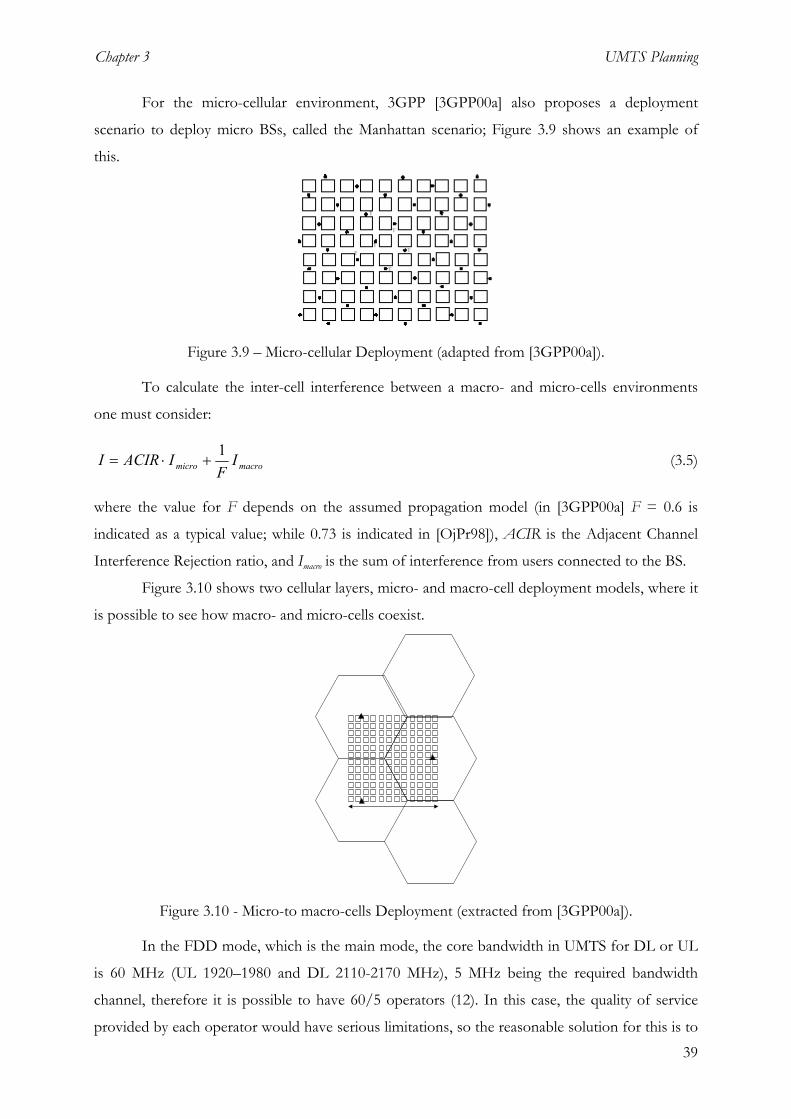
Chapter 3 UMTS Planning
For the micro-cellular environment, 3GPP [3GPP00a] also proposes a deployment
scenario to deploy micro BSs, called the Manhattan scenario; Figure 3.9 shows an example of
this.
Figure 3.9 – Micro-cellular Deployment (adapted from [3GPP00a]).
To calculate the inter-cell interference between a macro- and micro-cells environments
one must consider:
macromicro IF
IACIRI 1+⋅= (3.5)
where the value for F depends on the assumed propagation model (in [3GPP00a] F = 0.6 is
indicated as a typical value; while 0.73 is indicated in [OjPr98]), ACIR is the Adjacent Channel
Interference Rejection ratio, and Imacro is the sum of interference from users connected to the BS.
Figure 3.10 shows two cellular layers, micro- and macro-cell deployment models, where it
is possible to see how macro- and micro-cells coexist.
Figure 3.10 - Micro-to macro-cells Deployment (extracted from [3GPP00a]).
In the FDD mode, which is the main mode, the core bandwidth in UMTS for DL or UL
is 60 MHz (UL 1920–1980 and DL 2110-2170 MHz), 5 MHz being the required bandwidth
channel, therefore it is possible to have 60/5 operators (12). In this case, the quality of service
provided by each operator would have serious limitations, so the reasonable solution for this is to 39

UMTS Planning Chapter 3
provide 3 channels to each operator. With this solution, UMTS will have 4 potential operators
(the Portuguese case). For the TDD mode, in Portugal each operator has one single channel of 5
MHz.
3.4 Planning in STORMS
STORMS was a project in the ACTS programme partially funded by the European
Commission. The first outcome of STORMS was the identification of a new planning process
suited to the UMTS characteristic: multimedia services, new access schemes, and enhanced access
network architecture were some of the major issues considered in STORMS [MePi99].
Three major blocks can be identified in STORMS network strategy, Figure 3.11: the initial
dimensioning, the automatic radio coverage optimisation, and the refined dimensioning. Finally,
network performance can be assessed through a powerful UMTS simulator incorporated in the
STORMS platform. Note that the network optimisation process is based on a feedback process,
where for a given dimensioning the simulator performs coverage and capacity calculations, after
which an automatic and refined reconfiguration process begins, to be again evaluated in the new
network dimensioning. Note that the all process is based on demographical and geographical
information, due to traffic and propagation algorithm inputs.
Traffic analysis and
Preliminary Dimensioning
Automatic Radio Coverage Optimisation
Geographical Demographical
Refined Resource Dimensioning
Network Performance Evaluation
Propagation Modelling and
Radio Coverage Prediction
Intial Dimensioning
Automatic coverage optmisation
Refined dimensioning and performance evaluation
Figure 3.11 - Global network planning process (extracted from [MePi99]).
One of the major results of STORMS has been the development of a genetic optimisation
algorithm for the selection of optimal BS configurations (in terms of coverage). Figure 3.12 40

Chapter 3 UMTS Planning
shows the generic refined optimisation process for micro- and macro-cells, where, as inputs, it
receives traffic and propagation estimation results. These parameters are separated into two
groups, based on bit rate criteria, corresponding to low traffic macro-, and high traffic micro-
cells. Afterwards, the simulator checks the cell capacity, and decides if this cell dimensioning is
appropriated to traffic inputs; if it is not, it produces feedback to the optimisation process, until
capacity is adequate.
STORMS major result was the integration of several software modules, which were
integrated into a platform that can be used to study:
• Traffic density distributions on a per service and per layer (hierarchical structures) basis;
• Rough identification of cell sizes, essential to continue with a satisfactory radio planning;
• Automatic radio coverage optimisation and power planning;
• Dimensioning of a radio layer based on either FDD or TDD modes;
• Optimum allocation of RNCs and local exchanges, and identification of a cost effective
interconnecting network;
Carried &Overflow Traffic
Capacity is inadequate:Feed-Back to Coverage
Optimization
Radio Coverage FilesFor Micro/Macro Layers
Best Server Maps, PropagationMaps
Traffic Density FilesDescription: Service DependentInitially Segregated Traffic to
Micro/Macro Layers
Refined Traffic SegregationCriteria: Service Type
Collection of results
Micro-cell RefinedDimensioning
Macro-cell RefinedDimensioning
If Capacity is Adequate thenthe refined resource
dimensioning is completed
INPUT
High bitrateservices
Low bitrateservices
System Capacity CheckSystem Capacity Check
Capacity isadequate
Capacity is inadequate:Feed-Back to Coverage
Optimization
Carried &Overflow Traffic
Figure 3.12 - The generic refined planning process (extracted from [MePi99]).
41

UMTS Planning Chapter 3
• Optimum dimensioning of location and paging areas, including also "intelligent" paging
methods;
• Simulation of the final network configuration, in order to check the performance against the
initial requirements.
The optimisation process in STORMS is based on a feedback algorithm that converges to
an optimal network configuration in terms of radio coverage. This procedure inspired this thesis,
in order to get the optimal BS configuration based on:
• Network simulation (traffic generation, propagation and BS simulation);
• Network capacity verification, where a quality indicators analysis is perform, followed by a
decision for a new simulation or not;
• Network optimisation process, where new BS parameters are set, so that the network
converge, to an optimal configuration.
Figure 3.13 shows the main idea collected from STORMS.
NetworkSimulation
NetworkCapacity
Verification
NetworkOptimisation
Figure 3.13 - Network optimisation feedback process.
Note that the STORMS project has ended before all UMTS standards were finalised,
therefore, the real system characteristics were not considered by STORMS.
42

Chapter 4 Planning and Optimisation Tool
43
4 Planning and Optimisation Tool
4.1 Algorithm
As described in previous chapters, radio network planning is mainly based on three items:
traffic, propagation and services. In order to build a tool, capable of performing radio planning
and optimisation of a UMTS network [HaTo00], some major functional blocks are needed:
• Traffic generator based on traffic/service forecast tables;
• User behaviour and distribution for a given service area;
• Propagation model that fits the environment requirements;
• Description of services and radio interface characteristics.
After this, it is necessary to implement some computation algorithms to estimate or simulate the
UMTS radio network. In order to achieve good results, a real time traffic and propagation
simulator was developed.
A network planning and optimisation flow chart algorithm was designed, and all major
parameters were identified as the starting point of the planning and optimisation tool. One main
feature of this tool is that the optimisation process is automatic, which means that some network
planning parameters are changed automatically by the tool, with the objective of achieving the
optimum network design. In order to achieve this optimum configuration, sets of simulations are
performed, some major network quality indicators being analysed for each set; in this way, it is
possible to implement an algorithm that changes, from set to set, some parameters in the network
that directly or indirectly influence system capacity. The optimisation algorithm stops when the
required quality network goals are accomplish.
The major problems in GSM cellular planning tools are, in most cases, only related to
propagation issues. This fact is mainly due to the relatively simple radio interface
(FDMA/TDMA) of this type of networks: the number of channels allocated to each carrier is
deterministic, which means that the number of available channels is well know; therefore, it is
easy to establish a relation between traffic load, channels and blocking probability, usually via the
Erlang-B model [Yaco93].
The estimation of the number of channels in UMTS is not as linear as in GSM, which is
due to the quite different radio interface used (CDMA), as already described in previous chapters.
The number of channels depends on several factors: service (bit rate, traffic asymmetry, average
connection duration), power, multipath, interference, orthogonality level, distance between MT
and BS, number of users in the area and their propagation conditions, environment (urban,
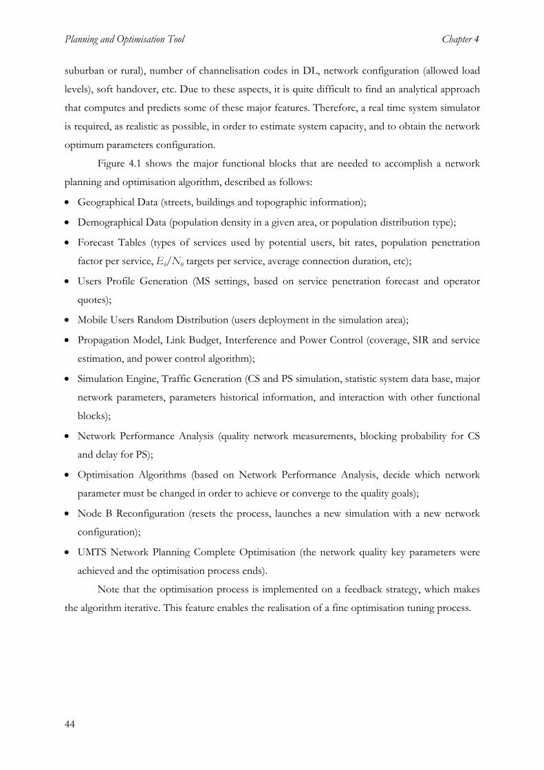
Planning and Optimisation Tool Chapter 4
44
suburban or rural), number of channelisation codes in DL, network configuration (allowed load
levels), soft handover, etc. Due to these aspects, it is quite difficult to find an analytical approach
that computes and predicts some of these major features. Therefore, a real time system simulator
is required, as realistic as possible, in order to estimate system capacity, and to obtain the network
optimum parameters configuration.
Figure 4.1 shows the major functional blocks that are needed to accomplish a network
planning and optimisation algorithm, described as follows:
• Geographical Data (streets, buildings and topographic information);
• Demographical Data (population density in a given area, or population distribution type);
• Forecast Tables (types of services used by potential users, bit rates, population penetration
factor per service, Eb/N0 targets per service, average connection duration, etc);
• Users Profile Generation (MS settings, based on service penetration forecast and operator
quotes);
• Mobile Users Random Distribution (users deployment in the simulation area);
• Propagation Model, Link Budget, Interference and Power Control (coverage, SIR and service
estimation, and power control algorithm);
• Simulation Engine, Traffic Generation (CS and PS simulation, statistic system data base, major
network parameters, parameters historical information, and interaction with other functional
blocks);
• Network Performance Analysis (quality network measurements, blocking probability for CS
and delay for PS);
• Optimisation Algorithms (based on Network Performance Analysis, decide which network
parameter must be changed in order to achieve or converge to the quality goals);
• Node B Reconfiguration (resets the process, launches a new simulation with a new network
configuration);
• UMTS Network Planning Complete Optimisation (the network quality key parameters were
achieved and the optimisation process ends).
Note that the optimisation process is implemented on a feedback strategy, which makes
the algorithm iterative. This feature enables the realisation of a fine optimisation tuning process.

Chapter 4 Planning and Optimisation Tool
PLANNING FLOW CHART
Forecast Tables
Users ProfileGeneration
Mobile UsersRandom
Distribution
Simulation EngineTraffic generation
Propagation Model,Link Budget,
Interference andPower Control
Node BReconfiguration
OptimisationAlgorithms
DemographicalData
GeographicalData
NetworkPerformance
Analysis
UMTS NetworkPlanning Complete
Optimisation
Figure 4.1 - UMTS planning and optimisation algorithm.
45
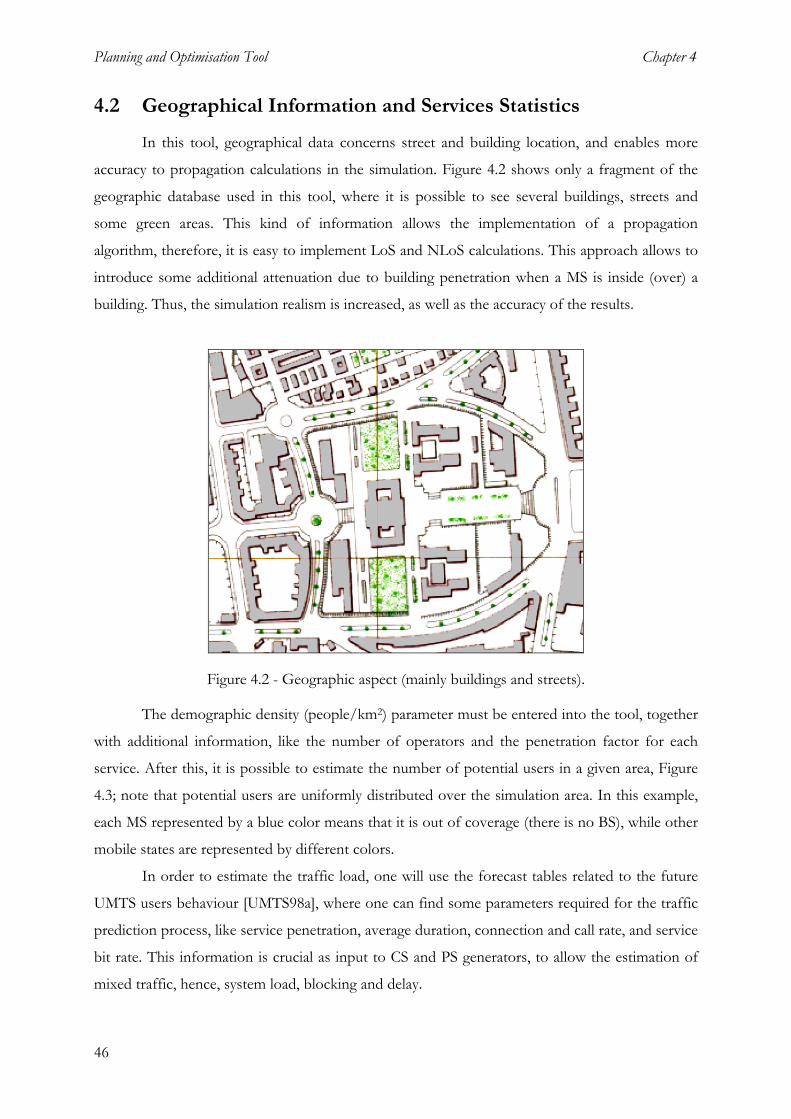
Planning and Optimisation Tool Chapter 4
4.2 Geographical Information and Services Statistics
In this tool, geographical data concerns street and building location, and enables more
accuracy to propagation calculations in the simulation. Figure 4.2 shows only a fragment of the
geographic database used in this tool, where it is possible to see several buildings, streets and
some green areas. This kind of information allows the implementation of a propagation
algorithm, therefore, it is easy to implement LoS and NLoS calculations. This approach allows to
introduce some additional attenuation due to building penetration when a MS is inside (over) a
building. Thus, the simulation realism is increased, as well as the accuracy of the results.
Figure 4.2 - Geographic aspect (mainly buildings and streets).
The demographic density (people/km2) parameter must be entered into the tool, together
with additional information, like the number of operators and the penetration factor for each
service. After this, it is possible to estimate the number of potential users in a given area, Figure
4.3; note that potential users are uniformly distributed over the simulation area. In this example,
each MS represented by a blue color means that it is out of coverage (there is no BS), while other
mobile states are represented by different colors.
In order to estimate the traffic load, one will use the forecast tables related to the future
UMTS users behaviour [UMTS98a], where one can find some parameters required for the traffic
prediction process, like service penetration, average duration, connection and call rate, and service
bit rate. This information is crucial as input to CS and PS generators, to allow the estimation of
mixed traffic, hence, system load, blocking and delay.
46
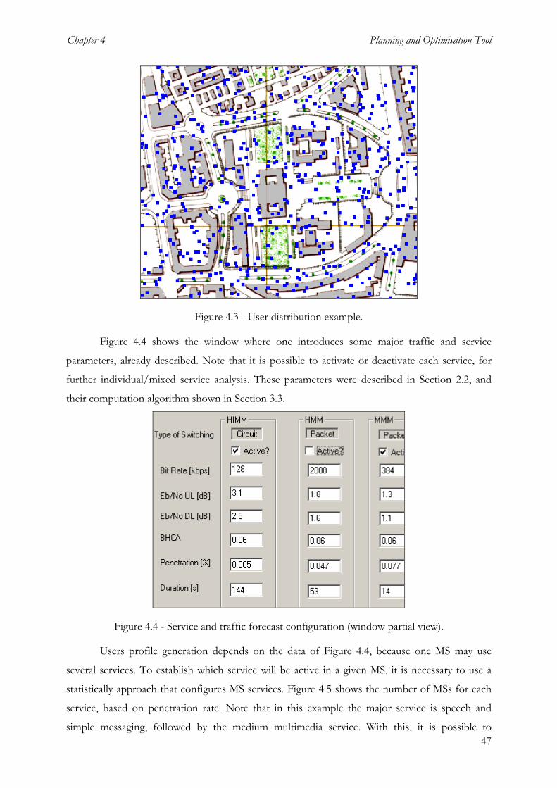
Chapter 4 Planning and Optimisation Tool
Figure 4.3 - User distribution example.
Figure 4.4 shows the window where one introduces some major traffic and service
parameters, already described. Note that it is possible to activate or deactivate each service, for
further individual/mixed service analysis. These parameters were described in Section 2.2, and
their computation algorithm shown in Section 3.3.
Figure 4.4 - Service and traffic forecast configuration (window partial view).
47
Users profile generation depends on the data of Figure 4.4, because one MS may use
several services. To establish which service will be active in a given MS, it is necessary to use a
statistically approach that configures MS services. Figure 4.5 shows the number of MSs for each
service, based on penetration rate. Note that in this example the major service is speech and
simple messaging, followed by the medium multimedia service. With this, it is possible to

Planning and Optimisation Tool Chapter 4
calculate the ratio between the number of services and the number of users. This is possible
because UMTS allows users to use several services in a simultaneous way. For example, if there is
100% of service penetration in all services the #Services/#Users parameter is 6.0, because all
MSs use all 6 available services. In the particular example of Figure 4.5, on average a MS uses
1.330 services.
Figure 4.5 - Users profile verification window.
4.3 Propagation Model and Link Budget
In radio network planning, it is vital to use a propagation model that satisfies the
environment and system parameters conditions. In order to fulfil these requirements the COST
231 Walfish-Ikegami [DaCo99] model was chosen, because it includes some major urban average
parameters, like street and building dimensions (see Section 2.3). Another reason to elect this
model is the cell type, since in this work only urban and micro-cell environments are considered.
Urban, suburban
Distance UE-NodeB
Frequency
Street width
PropagationModel
COST 231 W.I.
Node B Location
Building Separation
Building height
Geographical Info.
UE height
Path Loss
48

Chapter 4 Planning and Optimisation Tool
Figure 4.6 - COST 231 Walfish-Ikegami model parameters.
Figure 4.6 shows all parameters that the model needs to estimate the average path loss.
All these parameters are introduced by the tool user, except of course the MS (UE-User
Equipment according to the UMTS standard) location and distance between BS and the MS,
which is a variable value.
Each BS may have different propagation model parameters, which may be considered
more suitable for a given location area. The tool user may configure each BS through the window
shown in Figure 4.7. Note that not all parameters are introduced in this dialog box, since some
are introduced in the general simulation dialog or in BS configuration windows.
Figure 4.7 - Propagation parameters to each individual BS.
The link budget in UMTS introduces some additional concepts that must be considered
in the power budget calculations. For example, the receiver sensitivity depends on energy of bit
over noise, channel/system chip rate, user bit rate, and total estimated effective noise to allow the
estimation of Signal over Noise Ratio. Figure 4.8 shows several input parameters required to
perform the receiver power estimation algorithm already described in Section 2.3.2.
The link budget block performs a key role in the calculation of the power received by
MSs in DL. To estimate the power received by the user, in general terms, it is necessary to know
the following parameters: transmission power, antenna gain in a given direction, receiver antenna
49

Planning and Optimisation Tool Chapter 4
gain, additional attenuations (cable, body and car loss), and of course the path loss (given by the
propagation model) for each individual user.
Node B Noise Figure
Link Budget
Mobile Tx Power
Node B Gain
Eb/No
Interference Margin
Thermal Noise
MS Gain
Fading Margin
Soft HandoverGain
Additional Loss
Path Loss
Rx Power
Figure 4.8 - Link Budget block parameters
The power received by an user must be estimated based on a link budget. Figure 4.9
allows the tool user to introduce the following link budget parameters:
• Thermal Noise Density, which models the typical natural density noise;
• Receiver Noise Figure, characteristic of the equipment, attenuators, internal noise etc;
• Receiver Noise Density, which is the sum of thermal noise density and receiver noise figure,
the actual noise density at receiver input;
• Receiver Noise Power, the product of receiver noise density by the signal chip number;
• Interference Margin, the margin between noise and interference;
• Receiver Interference Power, estimated interference power based on interference margin and
noise power at the receiver;
• Total Effective Noise + Interference, which is a sum of interference and noise power at the
receiver;
• Max Mobile Tx Power, reserved for future work;
50

Chapter 4 Planning and Optimisation Tool
• Additional loss, the path loss increase, if a mobile is located inside a building, by user body
loss or by the BS cable loss.
Figure 4.9 - Link Budget parameters window.
Figure 4.10 - Sector coverage example (partial view). 51

Planning and Optimisation Tool Chapter 4
Figure 4.10 shows a coverage example with only one active sector, and only one active
service on the BS. Coverage is limited by transmitter power, antenna pattern, receiver service
sensitivity, and propagation parameters.
In UMTS, high bit rate services have a lower processing gain, therefore, the receiver
sensitivity level is higher, leading to smaller service coverage distances. Figure 4.11 shows multi-
services coverage, represented with different colour. As expected, coverage decreases when
services bit rate increases, since lower bit rates correspond to higher processing gain.
Figure 4.11 - Multi-service coverage in a single sector (partial view).
4.4 General Simulation Settings
Figure 4.12 shows the BS (Node B) major parameters that a user may configure. Each BS
may have up to 3 active sectors, and each one may be configured independently, e.g., by loading
different antenna radiation patterns.
Many other parameters are set here, like sector orientation (azimuth angle), expected or
typical orthogonality factor, number of channel codes reserved to signalisation, percentage of
channel codes reserved for soft handover, BS height (this parameter may automatically be
changed by the simulator algorithm optimisation process), frequency (for propagation model
reasons), manual BS repositioning, maximum transmitted power by the BS (to all users or to only
one), percentage of inter-cell interference coming from other BSs as a function of local
interference (aims to simulate the presence of other BSs, assuming a uniform load in the area),
and maximum allowed load factor, over which blocking and delay start to occur in the cell. This
latter parameter has a strong influence in network performance, because it is a threshold where
52

Chapter 4 Planning and Optimisation Tool
Radio Resource Management (RRM), starts to block or cause delay in connections. If the load
factor is low (below 0.4), the BS does not support many users, but is stable; otherwise, if it is set
at a high level, the BS allows many users, therefore, becoming very unstable, and starting to
generate many drop events.
.
Figure 4.12 - Individual Node B setup example.
Figure 4.13 - Antenna radiation pattern visualisation (horizontal plane).
53

Planning and Optimisation Tool Chapter 4
In Figure 4.13, it is possible to visualise information related to antenna pattern, supplied
by antenna suppliers. By using this, one may define the best antenna solution for each sector.
Some BS parameters cannot be changed by the tool user, but may be monitored, being
called “Node B properties”. The window shown in Figure 4.14 allows the tool user to view the
site identification, load factor in DL (UL not implemented), number of services connected (not
mobiles connected), current cell radius and current transmitted power.
Figure 4.14 - Individual Node B proprieties visualisation.
As it was mentioned before, some major parameters are introduced in a general
configuration window. Figure 4.15 shows a window where the tool user may configure several
main parameters at two different levels, as follows:
• Scenario and Simulation environment level:
o Number of operators (uniform distribution of population by operators is assumed), the
default value being 4, which is the Portuguese case;
o Output file directory to further analysis of results (where major internal parameters are
written in files, in order to analyse network behaviour and simulation optimisation
convergence steps, among others);
o Number of scrambling codes/Carrier, also reserved for future work, since it may be
possible to increase the number of scrambling codes for carrier (default value is 1);
o Carriers per operator, also for future work; essentially it may be used for increasing the
number of codes available, or for cell overlay analyses (default value is 1);
o Max number of BSs (#Node B max), which is the number of BSs that may be defined for
simulation memory management purposes;
o Population density, which is not the users density, but the potential population density in
the area (in the order of thousands/km2);
54

Chapter 4 Planning and Optimisation Tool
Figure 4.15 - General system configuration dialog window.
o Simulation step, being the interrupt routine processing period (typically, this parameter
depends on computer power processing capacity);
o Power Control, i.e., the number of times that power control is executed per second,
(default value is the standard one – 1500).
• MS and BS level:
o Antennas gain, for which, if no sector has been defined, a default value of 5 dBi for BSs
and 0 dBi for MSs will be considered;
o Node B initial radius, which may be automatically changed by the simulator optimisation
algorithm process (an expected value is recommended for simulation time reduction
proposes);
o Frequency, 2000 MHz being the recommended value (this value must be within the
propagation and UMTS boundaries);
o Total Tx Power, the maximum power transmitted by each BS in a single carrier (this
parameter, like others, may be changed in each BS individually);
55

Planning and Optimisation Tool Chapter 4
o Antenna initial height, which may be automatically changed by the simulator optimisation
algorithm process (an expected value is recommended for simulation time reduction
proposes), default value is 22 m.
4.5 Optimisation Settings
As already mentioned in previous chapters, this simulation tool, besides network planning
support, performs automatic network optimisation. In order that the tool user has control in this
process, some system thresholds, margins, and targets must be specified.
The dialog window presented in Figure 4.16 allows the tool user to establish the
optimisation and targets guidelines, as follows:
• Snapshot time means that after this simulation time some major network quality indicators
(blocking and delay) are analysed by the optimisation algorithm, and a decision on a proper
measure is taken in order that the simulation converges to the network quality targets,
described in Figure 4.17;
• The Node B height step means that, if the current network quality parameters are “near” the
network quality targets (based on a given criteria), the algorithm decides to change the BS
antennas height by this order of magnitude;
• The Node B location step (reserved to future work - not implemented) means that the BS
location may be optimised, therefore, site localisation may be changed by this order of
magnitude;
Figure 4.16 - Network optimisation parameters configuration window.
• Node B radius step means that, if current network quality parameters are “far” from the
network quality targets (based on a given criteria), the algorithm decides to change the cell
56
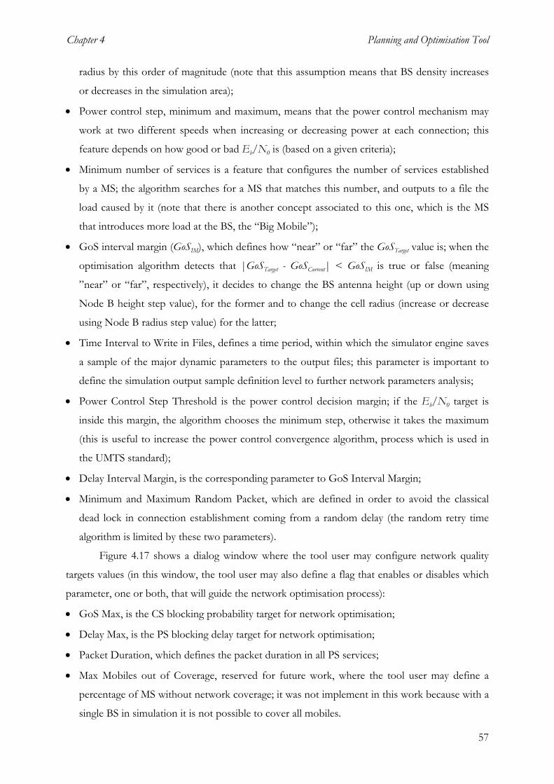
Chapter 4 Planning and Optimisation Tool
57
radius by this order of magnitude (note that this assumption means that BS density increases
or decreases in the simulation area);
• Power control step, minimum and maximum, means that the power control mechanism may
work at two different speeds when increasing or decreasing power at each connection; this
feature depends on how good or bad Eb/N0 is (based on a given criteria);
• Minimum number of services is a feature that configures the number of services established
by a MS; the algorithm searches for a MS that matches this number, and outputs to a file the
load caused by it (note that there is another concept associated to this one, which is the MS
that introduces more load at the BS, the “Big Mobile”);
• GoS interval margin (GoSIM), which defines how “near” or “far” the GoSTarget value is; when the
optimisation algorithm detects that |GoSTarget - GoSCurrent| < GoSIM is true or false (meaning
”near” or “far”, respectively), it decides to change the BS antenna height (up or down using
Node B height step value), for the former and to change the cell radius (increase or decrease
using Node B radius step value) for the latter;
• Time Interval to Write in Files, defines a time period, within which the simulator engine saves
a sample of the major dynamic parameters to the output files; this parameter is important to
define the simulation output sample definition level to further network parameters analysis;
• Power Control Step Threshold is the power control decision margin; if the Eb/N0 target is
inside this margin, the algorithm chooses the minimum step, otherwise it takes the maximum
(this is useful to increase the power control convergence algorithm, process which is used in
the UMTS standard);
• Delay Interval Margin, is the corresponding parameter to GoS Interval Margin;
• Minimum and Maximum Random Packet, which are defined in order to avoid the classical
dead lock in connection establishment coming from a random delay (the random retry time
algorithm is limited by these two parameters).
Figure 4.17 shows a dialog window where the tool user may configure network quality
targets values (in this window, the tool user may also define a flag that enables or disables which
parameter, one or both, that will guide the network optimisation process):
• GoS Max, is the CS blocking probability target for network optimisation;
• Delay Max, is the PS blocking delay target for network optimisation;
• Packet Duration, which defines the packet duration in all PS services;
• Max Mobiles out of Coverage, reserved for future work, where the tool user may define a
percentage of MS without network coverage; it was not implement in this work because with a
single BS in simulation it is not possible to cover all mobiles.

Planning and Optimisation Tool Chapter 4
Figure 4.17 - Network targets configuration window.
When quality indicator targets are reached after several snapshot simulations, the
optimisation process stops, and shows an optimum configuration network solution.
Figure 4.18 shows a window where the tool user in run time may monitor major
parameters, like traffic generation, MS state, delay, blocking and the optimisation process. The
information from top to bottom is the following:
• Real time, time passed since the simulation started;
• Simulated time, is the current simulation time, which is reset when it reaches the snapshot
time;
• Numbers of Node Bs and Users, quantity of equipment involved in simulation; note that the
number of MSs is a consequence of the population density, number of operators, and services
penetration;
• Circuit switching, total of circuit based services processed at current simulation time, number
of blocked and dropped circuit connections, blocking due to BS high load (GoS Power),
blocking due to lack of channel codes available (GoS Code), and the total blocking percentage
(GoS Total);
• Packet switching, total of packet based services processed at current simulation time, number
of blocked and dropped packet connections, delay due to BS high load (Power), delay due lack
of channel codes available (Code), and the total average delay [s/packet] (Total Delay);
58

Chapter 4 Planning and Optimisation Tool
Figure 4.18 - Dynamic network monitoring window.
• The Mobile Status box, gives information about the number of active services or idle in circuit
or packet connections;
• Voice Service, which is treated as a “special service” in this window, allowing to see the
estimated number of calls per hour, current average call duration, and traffic [Erlang];
• Performance parameters box, where the tool user may monitor some optimisation
evaluation/results: estimated coverage area, current cell radius, current BS height, number of
BSs per square kilometre (important to estimate the network cost for a given area), number of
59

Planning and Optimisation Tool Chapter 4
services connected to the BS, number of active users, relation between number of connected
services and number of MSs (note that this is possible because one single MS may use
different services simultaneously), BS load factor (which gives the relation between current
transmitted power to users and the maximum allowed total power), and finally the number of
DL channel codes available at the BS.
One should note that, when packet services are active, each MS may use higher layers in
the code tree, therefore, consuming several codes in lower layers, causing a lack of codes for
other incoming services.
4.6 Algorithms Validation
In order to validate some of the simulator main functionalities, namely propagation
model, link budget, and circuit and packet traffic random generators, some validations were
performed, which are presented in this section.
4.6.1 Propagation Model
A propagation model validation is essential, in order to achieve a reasonable accuracy in
propagation simulation results. Figure 4.19 shows the propagation model output for LoS, for two
frequencies (1900 and 2000 MHz), as a function of the distance between MS and BS. Note that
the validity range for this particularly section of the model is 20 to 200 m.
20 40 60 80 100 120 140 160 180 20060
65
70
75
80
85
90
95
Loss
[dB]
Distance [m]
1900 MHz 2000 MHz
Figure 4.19 - Computation results for COST 231 W.I. model for LoS.
60

Chapter 4 Planning and Optimisation Tool
It is important to note in Figure 4.19 that different frequencies (within the UMTS band)
do not have a major influence in signal attenuation. Therefore, one may assume that frequency
has a minor role in the system sensitivity and stabilisation.
The COST 231 W.I. model for NLoS environments produces quite different attenuation
results, Figure 4.20 presenting some of them. The black and red lines are almost 30 dB appart,
the main reason for this being BS and building roof top heights: if BS antenna height increases,
attenuation decreases for the same distance. Therefore, the BS antenna up and down movement
will affect the MS received signal conditions, and consequently the BS load, number of served
users, blocking and delay, etc.
0 1000 2000 3000 4000 5000
60
80
100
120
140
160
180
f = 2000 MHz, BS = 15 m, Buil.= 20 m f = 2000 MHz, BS = 30 m, Buil.= 20 m f = 1900 MHz, BS = 25 m, Buil.= 20 m f = 2000 MHz, BS = 25 m, Buil.= 20 m
Loss
[dB]
Distance [m] Figure 4.20 - Some computation results for COST 231 W.I. model in NLOS.
In the network optimisation process, it is important to identify several parameters that
may have or not considerable influence on system behaviour. Having in mind to identify these
parameters, several tests where performed. For example in Figure 4.21, attenuation was
computed as a function of distance and street width. Analysing these results, one can see that
street width variation does not have much influence in attenuation, therefore, one may conclude
that from the network optimisation point of view, street width is not relevant.
Figure 4.22 shows an attenuation surface as a function of distance, and difference
between building rooftop and BS height. Note that when BS antennas are below buildings
rooftop, there is a strong increase of attenuation, the turning point being when building rooftop
equals BS height. Therefore, one may conclude that the relation between BS and buildings
rooftop is very important to coverage estimation and BS load impact, and relevant to the
61

Planning and Optimisation Tool Chapter 4
optimisation process. BS antennas height is a good parameter for allowing a network tuning
quality/capacity process.
Figure 4.21 - Street width influence in NLoS attenuation.
Figure 4.22 - (Building Height-BS Height) influence in NLoS attenuation.
62
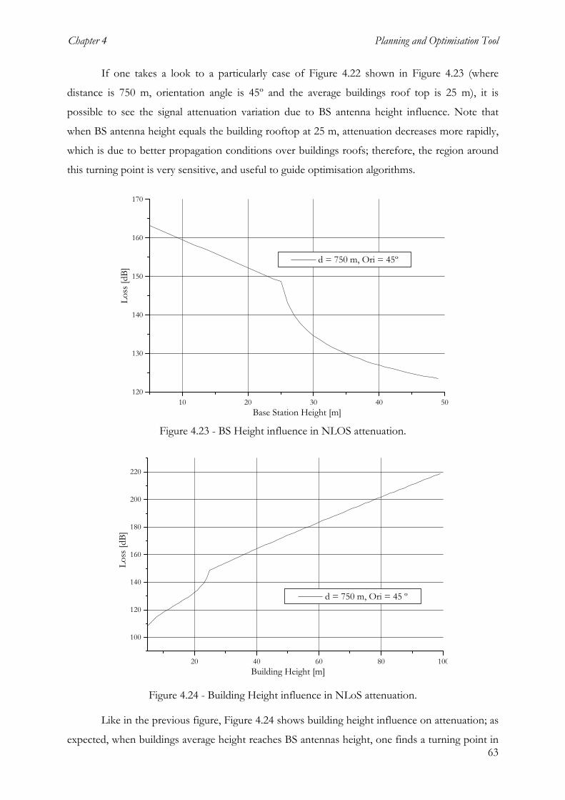
Chapter 4 Planning and Optimisation Tool
If one takes a look to a particularly case of Figure 4.22 shown in Figure 4.23 (where
distance is 750 m, orientation angle is 45º and the average buildings roof top is 25 m), it is
possible to see the signal attenuation variation due to BS antenna height influence. Note that
when BS antenna height equals the building rooftop at 25 m, attenuation decreases more rapidly,
which is due to better propagation conditions over buildings roofs; therefore, the region around
this turning point is very sensitive, and useful to guide optimisation algorithms.
10 20 30 40 50120
130
140
150
160
170
d = 750 m, Ori = 45º
Loss
[dB]
Base Station Height [m] Figure 4.23 - BS Height influence in NLOS attenuation.
20 40 60 80 100
100
120
140
160
180
200
220
d = 750 m, Ori = 45 º
Loss
[dB]
Building Height [m]
Figure 4.24 - Building Height influence in NLoS attenuation.
63
Like in the previous figure, Figure 4.24 shows building height influence on attenuation; as
expected, when buildings average height reaches BS antennas height, one finds a turning point in

Planning and Optimisation Tool Chapter 4
attenuation values. Therefore, one may conclude that if there is a need to decrease BS load factor
(total power level used in DL over maximum power at BS) in a constant cell radius environment,
one may increase a little bit the antennas height in order to decrease attenuation. On the other
hand, if one has very low GoS or Delay levels (meaning good values), one may decrease the BS
height, in order to reduce interference from and to other cells, decreasing load, and consequently
the blocking and delay factors.
This propagation model has another characteristic parameter, which is street orientation
angle. This is a correction parameter that weights the influence of street orientation relatively to
the propagation direction. Influence of street orientation angle in the propagation loss is clearly
shown in Figure 4.25, where two different curves for 200 and 400 m between MS and BS are
presented. Note that COST 231 propagation model in NLoS conditions is very distance sensitive,
therefore, cell radius or BS density in a given area is a major parameter that has to be optimised.
In other words, it is possible to manipulate the cell radius, assuming that when increasing or
decreasing cell radius a number of BSs per area modification is assumed, subsequently BS
capacity (load) is changed, until target values be accomplish.
0 50 100 150 200 250 300 350
108110112114116118120122124126128130132134136138140
Loss
[dB]
Street Orientation Angle [º]
Distance 400 m Distance 200 m
Figure 4.25 - Street orientation influence in NLoS attenuation.
4.6.2 Link Budget
Link Budget has a major role in the simulator, because it is here that several receiver
parameters are estimated, like MS received power, noise power, interference power, orthogonality
level, service sensitivity, additional losses and processing gain.
64
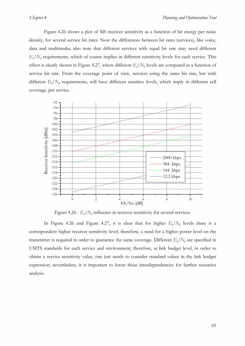
Chapter 4 Planning and Optimisation Tool
Figure 4.26 shows a plot of MS receiver sensitivity as a function of bit energy per noise
density, for several service bit rates. Note the differences between bit rates (services), like voice,
data and multimedia; also note that different services with equal bit rate may need different
Eb/N0 requirements, which of course implies in different sensitivity levels for each service. This
effect is clearly shown in Figure 4.27, where different Eb/N0 levels are computed as a function of
service bit rate. From the coverage point of view, services using the same bit rate, but with
different Eb/N0 requirements, will have different sensitive levels, which imply in different cell
coverage, per service.
0 2 4 6 8 10-126-124-122-120-118-116-114-112-110-108-106-104-102-100-98-96-94-92
Rece
iver
Sen
sitiv
ity [d
Bm]
2000 kbps 384 kbps 144 kbps 12.2 kbps
Eb/No [dB] Figure 4.26 - Eb/N0 influence in receiver sensitivity for several services.
In Figure 4.26 and Figure 4.27, it is clear that for higher Eb/N0 levels there is a
correspondent higher receiver sensitivity level, therefore, a need for a higher power level on the
transmitter is required in order to guarantee the same coverage. Different Eb/N0 are specified in
UMTS standards for each service and environment, therefore, at link budget level, in order to
obtain a service sensitivity value, one just needs to consider standard values in the link budget
expression; nevertheless, it is important to know these interdependencies for further scenarios
analysis.
65

Planning and Optimisation Tool Chapter 4
250 500 750 1000 1250 1500 1750 2000
-125
-120
-115
-110
-105
-100
-95
Rece
iver
Sen
sitiv
ity [d
Bm]
Bit Rate [kbit/s]
Eb/No = 5.0 dB Eb/No = 2.5 dB Eb/No = 1.0 dB
Figure 4.27 - Bit Rate influence on receiver sensitivity for Eb/N0 levels.
4.6.3 Random Generator
In discrete simulation environments, random variables represent a crucial role. In this
planning and optimisation UMTS tool, system traffic (CS and PS generation), users behaviour
and users distribution are implemented with random generators. Users distribution in a given area
is uniform distributed, as shown in Figure 4.3. Voice calls arrival rate follows a Poisson
distribution process. Poisson distribution is also valid for PS behaviour, since applications like e-
mail, file transfer or Internet browsing do not maintain long time connections.
Figure 4.28 compares a theoretical Poisson probability density function, represented by a
single blue line, with Poisson discrete simulator generator, represented by blue bars. Observing
this figure, one may conclude that the simulator generator is fair when compared to the
theoretical line. Note that when simulation time is increased this error will decrease, which is due
to an increase in the generator samples number.
Voice and videophone average call duration typically have a negative exponential
distribution. In this tool, all packets have a constant duration, nevertheless the tool user may
change it.
In conclusion one may say that the major and most sensitive random variables generators
functional blocks were validated.
66

Chapter 4 Planning and Optimisation Tool
67
Figure 4.28 - Poisson probability density generated by simulation (Bars) and analytically (Line).
4.7 Output Examples
In order to analyse the simulator results, it was necessary to implement a mechanism that
allows the analysis of main network parameters evaluation as a function of elapsed time. The
following figures are just plots of examples of these parameters.
Figures 4.29 to 4.34 show some major network parameter evolution, like BS load, GoS,
delay, cell radius, BS height and connections number. In these examples, the time resolution is 1
s, which means that 1 800 samples correspond to 0.5 hour of simulation snapshot. In this
example, the simulator optimisation process time (snapshot) is set to 0.5 hour; after this time, a
general reset is performed and a new snapshot is launched; this aspect is very clear when one
observes the following figures, where the decision and snapshot reset points are made at 1 800, 3
600 and 5 400 s.
Figure 4.29 shows the total BS load in DL, where all active connection loads are sum. The
BS load threshold in this example is 0.7, which means that equal or upper load values causes
blocking or delay at the BS when new connections arrive; nevertheless, the BS allows upper
values, due to power control in MSs that are already connected.
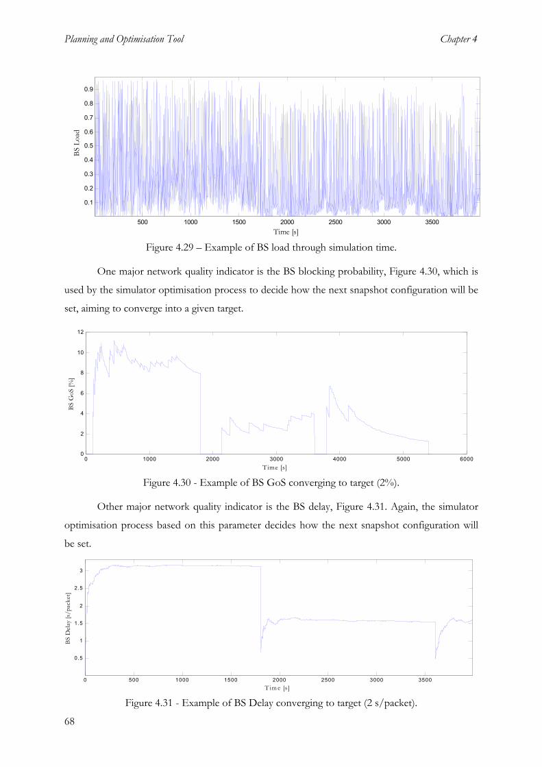
Planning and Optimisation Tool Chapter 4
68
500 1000 1500 2000 2500 3000 3500
0.1
0.2
0.3
0.4
0.5
0.6
0.7
0.8
0.9
BS L
oad
Time [s] Figure 4.29 – Example of BS load through simulation time.
One major network quality indicator is the BS blocking probability, Figure 4.30, which is
used by the simulator optimisation process to decide how the next snapshot configuration will be
set, aiming to converge into a given target.
0 1000 2000 3000 4000 5000 60000
2
4
6
8
10
12
BS G
oS [%
]
T ime [s] Figure 4.30 - Example of BS GoS converging to target (2%).
Other major network quality indicator is the BS delay, Figure 4.31. Again, the simulator
optimisation process based on this parameter decides how the next snapshot configuration will
be set.
0 500 1000 1500 2000 2500 3000 3500
0.5
1
1.5
2
2.5
3
BS D
elay
[s/p
acke
t]
T im e [s] Figure 4.31 - Example of BS Delay converging to target (2 s/packet).

Chapter 4 Planning and Optimisation Tool
The convergence/optimisation in this example is very clear: in the second simulation (1
800 to 3 600 s), blocking and delay levels decrease relatively to the first one (0 to 1 800 s), which
is due to cell radius decrease Figure 4.32. This reduction was decided by the optimisation process,
based on first simulation results (which present values clearly above targets). Note that in Node B
cell radius plot Figure 4.32, one may see some network convergence from 900 to 850 m, which
implies a decrease on the average GoS and packet delay.
0 1000 2000 3000 4000 5000 6000840
850
860
870
880
890
900
Cell
Radi
us [m
]
T im e [s ] Figure 4.32 - Example of cell radius converging to optimum value.
Note that cell radius is an extremely important parameter, because, based on this, an
operator may estimate the BS density, therefore, the cost, offered capacity and network quality.
In Figure 4.33, the BS height convergence is presented. This parameter also converges
automatically to an optimum value. Based on this value, an operator may estimate the BS antenna
height, in order to accomplish the quality targets.
1000 2000 3000 4000 5000 6000
20
20.5
21
21.5
22
BS A
nten
na H
eigh
t [m
]
T ime [s] Figure 4.33 - Example of BS antenna height converging to the optimum value.
As already mentioned, a MS may use more than one service, therefore the number of
active connections may be higher than the number of active MSs. This information is shown in
Figure 4.34.
Figures 4.35 to 4.40 show all six individual UMTS Forum defined services, where each
service load is plotted. It is possible to observe which services have more influence on the
network (load). The HMM and S services present higher load, due to high bit rate service (2000
kbps) and to high penetration percentage, respectively. Also note that, on average, these 69

Planning and Optimisation Tool Chapter 4
individual service loads decrease/increase depends on decisions performed by the optimisation
process between snapshots.
0 1000 2000 3000 4000 50000
5
10
15
20
25
# C
onne
cted
Ser
vice
s
T im e [s ] Figure 4.34 - Example of number of connected services.
Load depends greatly of service bit rate, service penetration and average connection time,
therefore, some services offer more or less load. Figure 4.35 shows the speech load; although this
service has a low bit rate, it is the most used by users, hence, it is an important service from the
BS load point of view.
500 1000 1500 2000 2500 3000 3500 4000 4500 5000 55000
0.1
0.2
0.3
0.4
0.5
0.6
S Se
rvic
e Lo
ad
T ime [s] Figure 4.35 - Example of S service load.
0 500 1000 1500 2000 2500 3000 3500 4000 4500 50000
0.1
0.2
0.3
0.4
0.5
0.6
0.7
0.8
0.9
HM
M S
ervi
ce L
oad
T ime [s] Figure 4.36 - Example of HMM service load.
70

Chapter 4 Planning and Optimisation Tool
As expected, HMM service has a huge impact on the BS load, mainly due to high bit rate.
Figure 4.36 clearly shows this aspect, where this service is responsible for leading the BS to its
power and channel code limits.
Based on the UMTS Forum, the HIMM penetration forecast value is expected to be very
low, therefore, the impact on the BS load is expected to be low as well, as Figure 4.37 shows.
500 1000 1500 2000 2500 3000 3500 4000 4500 50000
0.05
0.1
0.15
0.2
0.25
0.3
0.35
0.4
HIM
M S
ervi
ce L
oad
T ime [s] Figure 4.37 - Example of HIMM service load.
The SD, Figure 4.38, and SM, Figure 4.39, have the same bit rate, but different
penetration values. Due to this, SD and SM put quite different loads into the BS; besides this, it is
important to remember that SD is CS while SM is PS.
0 500 1000 1500 2000 2500 3000 3500 4000 4500 50000
0.002
0.004
0.006
0.008
0.01
0.012
0.014
0.016
0.018
0.02
SD S
ervi
ce L
oad
T ime [s] Figure 4.38 - Example of SD service load.
0 500 1000 1500 2000 2500 3000 3500 4000 4500 50000
0.05
0.1
0.15
SM S
ervi
ce L
oad
T ime [s] Figure 4.39 - Example of SM service load.
71

Planning and Optimisation Tool Chapter 4
Figure 4.38 shows clearly the SD CS nature, where connections are maintained for a long period
of time, compared to SM, Figure 4.39, which is a PS based service.
MMM is characterised mainly by a high bit rate and its PS nature. Due to these features,
the fast power control mechanism leads this service to high load levels, like shown in Figure 4.40.
0 500 1000 1500 2000 2500 3000 3500 4000 4500 50000
0.1
0.2
0.3
0.4
0.5
0.6
0.7
0.8
0.9
MM
M S
ervi
ce L
oad
T ime [s] Figure 4.40 - Example of MMM service load.
At the BS 512 channel codes are available, which corresponds to one code tree
[3GPP00c]. Each different bit rate service uses different SF levels; for example, a basic 15 kbps
link uses a SF of 512 (1 channel code), while a 1960 kbps link uses a SF of 4 (128 channel code).
Therefore, the number of available channel codes gives the BS load from the channels point of
view. In simulations, it is assumed that 128 channel codes are used for signalling purposes and
that 30 % (153 channels) are reserved for soft handover, therefore, a maximum of 230 channel
codes are available for traffic. In Figure 4.41, a zoom of this parameter is shown, where it is easy
to observed the arrival of high bit rate connections, mostly PS based services.
1300 1350 1400 1450 1500 1550 1600 1650 1700 1750 18000
50
100
150
200
# C
odes
T ime [s] Figure 4.41 - Example of number of available channel codes.
As explained before, blocking is also due to the lack of channel codes. Figure 4.42 shows
an example of blocking probability, due only to channel codes unavailability (mainly high bit rate
service dependent).
72

Chapter 4 Planning and Optimisation Tool
73
2400 2500 2600 2700 2800 2900 3000 31000
0.2
0.4
0.6
0.8
1
1.2
1.4
1.6
1.8
2G
oS (c
odes
) [%
]
T ime [s] Figure 4.42 - Example of blocking due to lack of channel codes.
2400 2500 2600 2700 2800 2900 3000 3100
0
0.5
1
1.5
2
2.5
GoS
(pow
er) [
%]
Time [s] Figure 4.43 - Example of blocking only due to lack of power.
Like in the previous example, Figure 4.43 shows the blocking probability example, caused
by the power load threshold, meaning that when the BS load reaches a given mark (i.e. 70 %) new
connections originated by CS services will be blocked. Note that the total blocking probability is
the sum of these two contributions.
PS based services will suffer delay on the network. In order to understand how delay
depends on BS resources, the simulator distinguishes the total delay from two sources, power and
codes. In Figure 4.44, an output example is shown where it is possible to observe the impact that
power has on delay; in this particular example, it is also possible to see simulation convergence
between the simulation reset points. As in the previous parameter, it is possible to observe the
same points in Figure 4.45. Comparing Figure 4.44 and Figure 4.45, it is clear that delay is more
sensitive to channel codes resource rather than power, because most of PS services (high bit
rates) use the low levels on the code tree, which prevents the use of many channel codes.

Planning and Optimisation Tool Chapter 4
74
0 1000 2000 3000 4000 50000
2
4
6
8
10
12
Del
ay (p
ower
) [%
]
T ime [s] Figure 4.44 - Example of BS delay percentage due to lack of power.
0 1000 2000 3000 4000 50000
5
10
15
20
25
30
35
40
Del
ay (c
ode)
[%]
T im e [s]
Figure 4.45 - Example of BS delay due to lack of channel codes.
In order to verify the power control algorithm, an internal simulator parameter was
created that is sensitive to a “special MS”, and reveals the signal level received by this MS. This
“special MS” is selected based on the following criteria: among all MSs, the one that is currently
using more power resources at the BS is selected. An example of this output parameter is shown
in Figure 4.46. Note that this parameter considers several MSs, through simulation time.
2300 2400 2500 2600 2700 2800 2900 3000 3100
-120
-110
-100
-90
-80
-70
-60
Rx le
vel [
dBm
]
T ime [s] Figure 4.46 - Example of power control on special mobile receiver.
Using this tool, it is possible to monitor the optimisation process and all the main
parameters (i.e. quality indicators, network configuration parameters), enabling the visualisation

Chapter 4 Planning and Optimisation Tool
75
of instantaneous network configurations and also average results, providing a detailed analysis on
network parameters impact and sensitivity (users/services/network). Besides UMTS radio
interface, this tool also produces an optimum cell radius. The optimisation process used in this
tool is a very interesting feature that allows the user to focus his work onto scenario definition,
entrusting into the automatic process the planning work, however, it is possible to control this
process and all other parameters.
Compared to other simulation tools, this one presents good and interesting results using
low computational resources, mainly due to the simplified algorithm approach (only one BS,
expanded in future work).
Multi service generation was performed using source models, for voice, a classical voice
model was implemented (Poisson arrival process and exponential call duration), to simulate
packets an ON-OFF model was implemented. For data, a packet approach is taken, with fixed
length ones.
The main algorithms used in this tool were validated, for example: propagation models,
link budget, user generation, users profile generation, source models and output results.
This tool intends to give trends for major parameters, based on a simple approach, and
with a low computation load.


Chapter 5 Scenarios Analysis
5 Analysis of Scenarios
5.1 Scenarios, Definition
Cellular planning is quite scenario dependent, therefore, a scenario that represents an
acceptable or typical service area is required, aiming to accomplish good results. In cellular
networks, there are three well-known scenarios: rural, suburban and urban. The most important is
the urban one, followed by the suburban, and finally the rural; this order is due to traffic load
(population density), propagation issues, and scenario network dependency.
A differentiated urban scenario must be analysed in order to include several urban
aspects. After searching this kind of scenario in the Lisbon area, a specific area was selected,
Figure 5.1, which has large avenues, squares, rectangular urban architecture, and a relative
constant building height. This area represents a typical urban environment that mixes several
major propagation and services aspects. From the propagation modelling point of view, this
environment has also another advantage: it fits the propagation model parameters’ specifications.
In order to easily distinguish streets from buildings borders, since the simulator can process this
information (as already shown in Chapter 4), a simplification of the digital image was performed.
Figure 5.1 - Partial simulated scenario (adapted from [CMLi01]).
Any major city is characterised by different population densities in its different areas,
which is due to several urban aspects, like industry location, airports, huge commercial centres, 77

Scenarios Analysis Chapter 5
large business areas, residential areas, historical and tourist areas, sport zones, etc. Cellular
networks, like GSM, adapt their BS location as a function of these densities, in order to provide
capacity and coverage to users. Figure 5.2 shows Lisbon population density map, where one can
see that the larger population densities are located in business and historical areas downtown
(during day time).
Figure 5.2 - Population density in Lisbon (adapted from [CMLi01]).
In GSM planning (voice service), it is possible to predict the traffic density load in Erlang
per km2, generated by users, and then establish a relation between users offered traffic and
network traffic capacity, leading directly to the BS density. In UMTS planning, this concept it not
valid, as already discussed in previous chapters, therefore, a system simulator is required, in order
to estimate some major UMTS network parameters, like cell range, among many others.
Simulations depend greatly on all parameters, but if there is a change on two or more
parameters in the simulation set, certainly becomes impossible to distinguish the influence in the
system sensitivity analysis from one particularly parameter to another. In order to understand the
impact that each parameter has on network behaviour, it is indispensable to perform an
individual study, assuming that all others are constant. So, it is necessary to define a reference
scenario from which it is possible to study the network dependency on system and scenario
parameters. For all services identified by the previously mentioned UMTS-Forum scenario, Table
5.1 presents some major parameters and their respective values [UMTS98a]. Note that Eb/N0
target values were extracted from ETSI [ETSI00]. Tables 5.1 and 5.2 show all simulation default
78

Chapter 5 Scenarios Analysis
79
parameters and values (UMTS Forum scenario), a description of these being found in Chapter 4.
Exceptions to these assumptions are mentioned in explicit form.
Table 5.1 - Default individual service settings for urban pedestrian and vehicular (year 2005).
Service HMM MMM HIMM SM SD S
Bit rate [kbps] 2000 384 128 14 14 12
Av. Connec.. Time [s] 53 14 144 30 156 60
Penetration [%] 4.7 7.7 0.5 25 10 60
Eb/N0 DL [dB] 1.6 1.1 2.5 1.2 1.2 6.1
Switching PS PS CS PS CS CS
Table 5.2 - Default general parameters settings.
Simulator Parameters Value Simulator Parameters Value
Initial BS Height [m] 22 3 Sectors 90º, 210º
330º
Buildings Height [m] 20 Snapshot Time [s] 900
Buildings Separation [m] 60 BS Height Step [m] 1
Streets Width [m] 30 Cell radius Step [m] 25
MS Height [m] 1.5 Power Control Freq. [Hz] 500
Urban Type Metro.
Centre Power Control Step Min. [%] 10
Frequency [MHz] 2000 Power Control Step Max. [%] 50
Orthogonality Factor 0.5 Power Control Step Marg. [dB] 5
Signalisation channel codes 128 Blocking Margin [%] 2
Soft Handover [%] 30 Delay Margin [s] 2
BS Max. Tx Power [W] 10 Blocking Target [%] 2
Inter Interference Load [%] 30 Delay Target [s] 2
BS Max. Load Factor 0.7 Retry Time Min. [s] 3
Packet Duration [s] 1 Retry Time Max. [s] 10
Thermal Noise Density [dB/Hz] -174 Receiver Noise Figure [dB] 5
Receiver Noise Density [dB/Hz] -169 Receiver Noise Power [dBm] -103
Interference Margin [dB] 3 Building Penetration Lost [dB] 10
# Operators 4 Population Density [pop/km2] 10 000
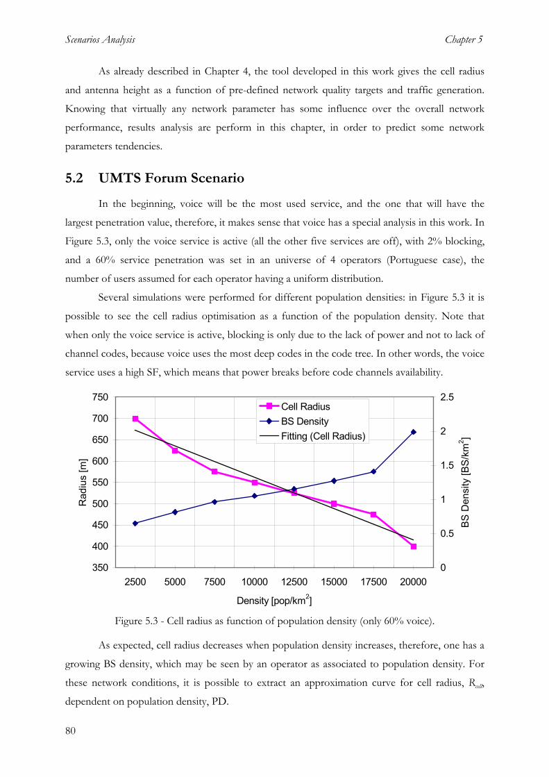
Scenarios Analysis Chapter 5
As already described in Chapter 4, the tool developed in this work gives the cell radius
and antenna height as a function of pre-defined network quality targets and traffic generation.
Knowing that virtually any network parameter has some influence over the overall network
performance, results analysis are perform in this chapter, in order to predict some network
parameters tendencies.
5.2 UMTS Forum Scenario
In the beginning, voice will be the most used service, and the one that will have the
largest penetration value, therefore, it makes sense that voice has a special analysis in this work. In
Figure 5.3, only the voice service is active (all the other five services are off), with 2% blocking,
and a 60% service penetration was set in an universe of 4 operators (Portuguese case), the
number of users assumed for each operator having a uniform distribution.
Several simulations were performed for different population densities: in Figure 5.3 it is
possible to see the cell radius optimisation as a function of the population density. Note that
when only the voice service is active, blocking is only due to the lack of power and not to lack of
channel codes, because voice uses the most deep codes in the code tree. In other words, the voice
service uses a high SF, which means that power breaks before code channels availability.
350
400
450
500
550
600
650
700
750
2500 5000 7500 10000 12500 15000 17500 20000
Density [pop/km2]
Rad
ius
[m]
0
0.5
1
1.5
2
2.5
BS D
ensi
ty [B
S/km
2 ]
Cell RadiusBS DensityFitting (Cell Radius)
Figure 5.3 - Cell radius as function of population density (only 60% voice).
As expected, cell radius decreases when population density increases, therefore, one has a
growing BS density, which may be seen by an operator as associated to population density. For
these network conditions, it is possible to extract an approximation curve for cell radius, Rcell,
dependent on population density, PD.
80
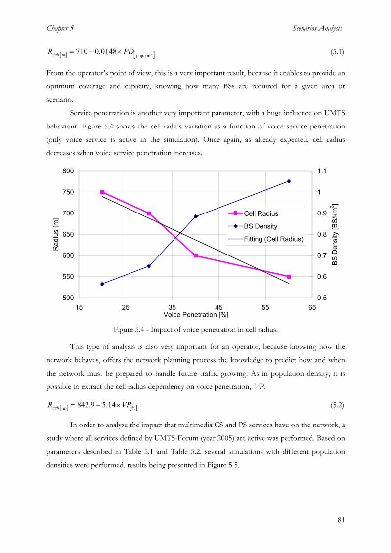
Chapter 5 Scenarios Analysis
[ ] [ 2pop/km 0148.0710 PDR mcell ]×−= (5.1)
From the operator’s point of view, this is a very important result, because it enables to provide an
optimum coverage and capacity, knowing how many BSs are required for a given area or
scenario.
Service penetration is another very important parameter, with a huge influence on UMTS
behaviour. Figure 5.4 shows the cell radius variation as a function of voice service penetration
(only voice service is active in the simulation). Once again, as already expected, cell radius
decreases when voice service penetration increases.
500
550
600
650
700
750
800
15 25 35 45 55 65Voice Penetration [%]
Rad
ius
[m]
0.5
0.6
0.7
0.8
0.9
1
1.1
BS D
ensi
ty [B
S/km
2 ]
Cell Radius
BS Density
Fitting (Cell Radius)
Figure 5.4 - Impact of voice penetration in cell radius.
This type of analysis is also very important for an operator, because knowing how the
network behaves, offers the network planning process the knowledge to predict how and when
the network must be prepared to handle future traffic growing. As in population density, it is
possible to extract the cell radius dependency on voice penetration, VP.
[ ] [ ]%m 14.59.842 VPRcell ×−= (5.2)
In order to analyse the impact that multimedia CS and PS services have on the network, a
study where all services defined by UMTS-Forum (year 2005) are active was performed. Based on
parameters described in Table 5.1 and Table 5.2, several simulations with different population
densities were performed, results being presented in Figure 5.5.
81

Scenarios Analysis Chapter 5
350
400
450
500
550
600
0 5000 10000 15000 20000Density [pop / km2]
Rad
ius
[m]
Figure 5.5 - Population density impact on cell radius.
Comparing to the “only voice” scenario (Figure 5.3), these results show a clear reduction
in the cell radius, which is due to multimedia impact on cell load. Again, a relation between cell
radius and population density was extracted.
[ ] [ 2pop/km m 01.0575 PDRcell ×−= ] (5.3)
In order to estimate the different weight that population density and mixed services has on cell
radius ‘or network cost’, one may compare (5.1) and (5.3), and conclude that the population
density influence is quite similar (in terms of slope), but that there is about 140 m offset, which is
due to mixed services impact on network capacity.
Table 5.3 - Service penetration forecast values based on UMTS Forum, for various years.
Penetration [%] Service
2003 2005 2007 2010
HIMM 0.1 0.5 2.9 5.3
HMM 2.0 4.7 11.4 18.0
MMM 2.6 7.7 12.9 18.0
SD 10.0 10.0 10.0 10.0
SM 17.5 25.0 32.5 40.0
S 52.5 60.0 67.5 75.0
Total 84.6 107.9 137.1 166.3
Average
[Ser./user] 1.28 1.39 1.61 1.73
82

Chapter 5 Scenarios Analysis
System sensitivity to different service penetration values is an important result, because it
is possible to predict the future network behaviour. In order to do so, forecast penetration values
for each service based on the UMTS Forum predictions were established for the years 2005 and
2010, Table 5.3. Note that values for years 2003 and 2007 were extra/interpolated, based on 2005
and 2010 service penetration ones [UMTS98a]. Note also that one user has the possibility to
activate more than one service simultaneously, therefore, the average number of services per user
was calculated; as expected, this parameter raises along the years. Furthermore, the total
penetration (bottom row) represents the sum of all services penetration (if all users would have all
services, the total would be 600% and the average 6.0).
Figure 5.6 shows some simulation results, using values presented in Table 5.3. As
expected, the optimum cell radius decreases along the years, due to capacity needs (i.e., expected
growing number of users).
300
350
400
450
500
550
2002 2003 2004 2005 2006 2007 2008 2009 2010 2011Years
Rad
ius
[m]
SimulationFitting
Figure 5.6 - Services penetration growing impact on the network.
Equation (5.4), extracted from Figure 5.6, suggests how the network behaves as a
function of service penetration in the future, where Y represents the year.
[ ] ( )20036.22505m −×−= YRcell (5.4)
In order to analyse the impact that individual high bit rate PS services (384 kbps and 2
Mbps) have on the network, some system simulations where performed, adding one of these two
services to voice, in independent simulations; the voice service penetration was fixed to 60 %.
Results are shown in Figure 5.7 and Figure 5.8, where it is possible to observe a strong cell radius
reduction due to high bit rate impact (0 % to 20% service penetration). For lower penetration
values, a more linear radius decrease curve is observed, always optimised by BS antenna height
corrections, aiming to optimise system performance. Comparing Figure 5.4 with Figure 5.7, one
may say that the voice service scenario has about less 200 m radius, when mixed with the 384
kbps service.
83

Scenarios Analysis Chapter 5
390410430450470490510530550570
0 20 40 60384 kbps Service Penetration [%]
Rad
ius
[m]
Simulation
Fitting
Figure 5.7 - Impact on cell radius, due to 384 kbps penetration variation over voice.
Again, using these results, it is possible to establish an analytical relation between 384
kbps service penetration, SP and cell radius:
[ ] [ ] [2
%384%384m 05.02.5546 SPSPRcell ×−×−= ] (5.5)
As expected, higher service penetration values introduce additional load into the BS at the
power level, and a strong reduction on channel codes availability. When high bit rates are active,
higher power levels are required, and many codes are used, causing delay and blocking at the BS,
therefore, a cell radius reduction is required (through a user reduction scheme), in order to
maintain system quality targets in a given range (Table 5.1).
Figure 5.8 presents the HMM service (2000 kbps) penetration impact on BS load, which
is huge as expected. It leads the cell radius to 150 m when HMM reaches 60% penetration, which
means that the system reaches indoor environment characteristics, as already anticipated by other
studies (mentioned in previous chapters).
75
175
275
375
475
575
0 10 20 30 40 50 62000 kb
0ps Service Penetration [%]
Rad
ius
[m] Simulation
Fitting
Figure 5.8 - Impact on cell radius, due to 2000 kbps penetration variation over voice.
84
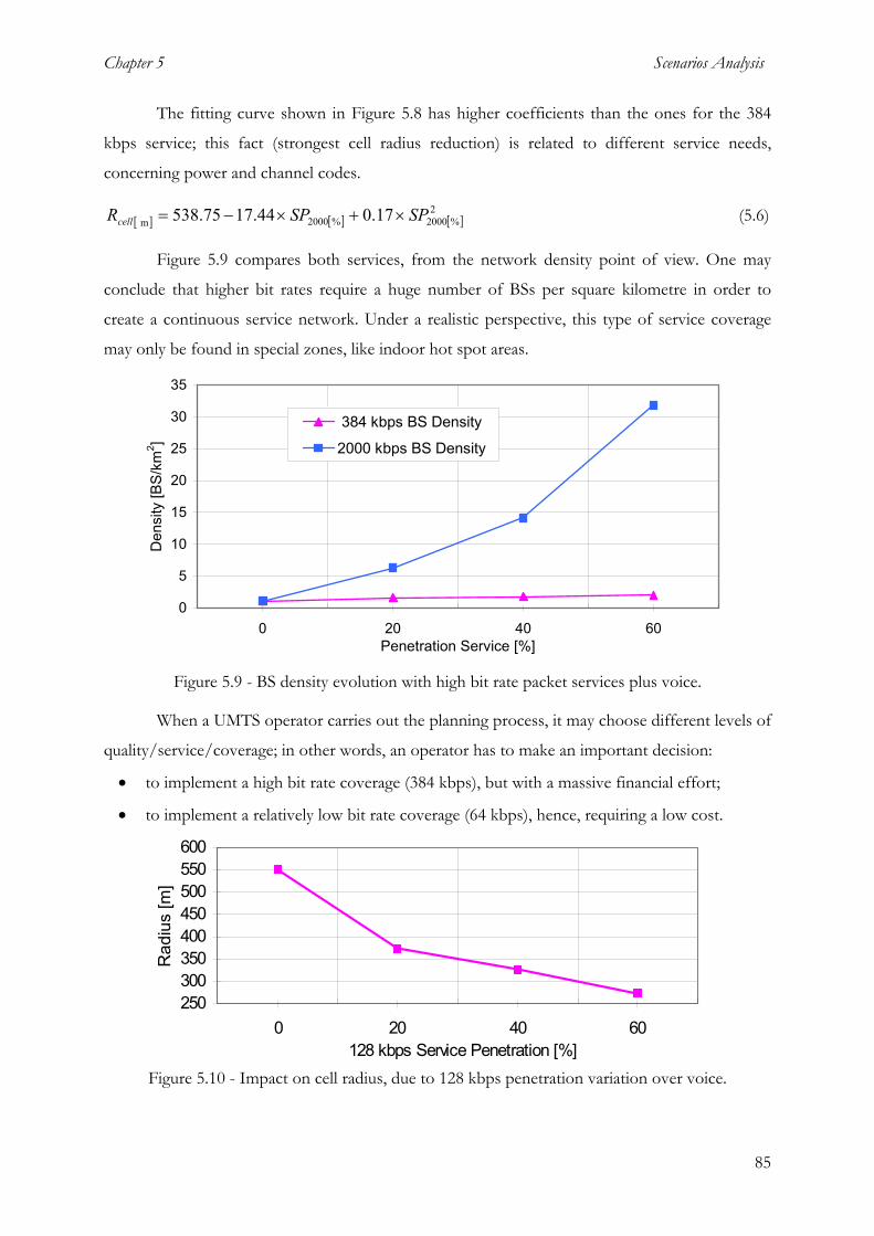
Chapter 5 Scenarios Analysis
The fitting curve shown in Figure 5.8 has higher coefficients than the ones for the 384
kbps service; this fact (strongest cell radius reduction) is related to different service needs,
concerning power and channel codes.
[ ] [ ] [2
%2000%2000m 17.044.1775.538 SPSPRcell ×+×−= ] (5.6)
Figure 5.9 compares both services, from the network density point of view. One may
conclude that higher bit rates require a huge number of BSs per square kilometre in order to
create a continuous service network. Under a realistic perspective, this type of service coverage
may only be found in special zones, like indoor hot spot areas.
0
5
10
15
20
25
30
35
0 20 40 60Penetration Service [%]
Den
sity
[BS/
km2 ]
384 kbps BS Density
2000 kbps BS Density
Figure 5.9 - BS density evolution with high bit rate packet services plus voice.
When a UMTS operator carries out the planning process, it may choose different levels of
quality/service/coverage; in other words, an operator has to make an important decision:
• to implement a high bit rate coverage (384 kbps), but with a massive financial effort;
• to implement a relatively low bit rate coverage (64 kbps), hence, requiring a low cost.
250300350400450500550600
0 20 40 60128 kbps Service Penetration [%]
Rad
ius
[m]
Figure 5.10 - Impact on cell radius, due to 128 kbps penetration variation over voice.
85
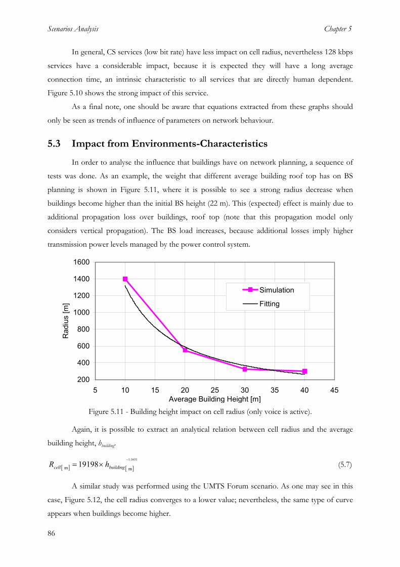
Scenarios Analysis Chapter 5
In general, CS services (low bit rate) have less impact on cell radius, nevertheless 128 kbps
services have a considerable impact, because it is expected they will have a long average
connection time, an intrinsic characteristic to all services that are directly human dependent.
Figure 5.10 shows the strong impact of this service.
As a final note, one should be aware that equations extracted from these graphs should
only be seen as trends of influence of parameters on network behaviour.
5.3 Impact from Environments-Characteristics
In order to analyse the influence that buildings have on network planning, a sequence of
tests was done. As an example, the weight that different average building roof top has on BS
planning is shown in Figure 5.11, where it is possible to see a strong radius decrease when
buildings become higher than the initial BS height (22 m). This (expected) effect is mainly due to
additional propagation loss over buildings, roof top (note that this propagation model only
considers vertical propagation). The BS load increases, because additional losses imply higher
transmission power levels managed by the power control system.
200
400
600
800
1000
1200
1400
1600
5 10 15 20 25 30 35 40Avera
45ge Building Height [m]
Rad
ius
[m]
Simulation
Fitting
Figure 5.11 - Building height impact on cell radius (only voice is active).
Again, it is possible to extract an analytical relation between cell radius and the average
building height, hbuilding.
[ ] [ ]1631.1
m m 19198−
×= buildingcell hR (5.7)
A similar study was performed using the UMTS Forum scenario. As one may see in this
case, Figure 5.12, the cell radius converges to a lower value; nevertheless, the same type of curve
appears when buildings become higher.
86
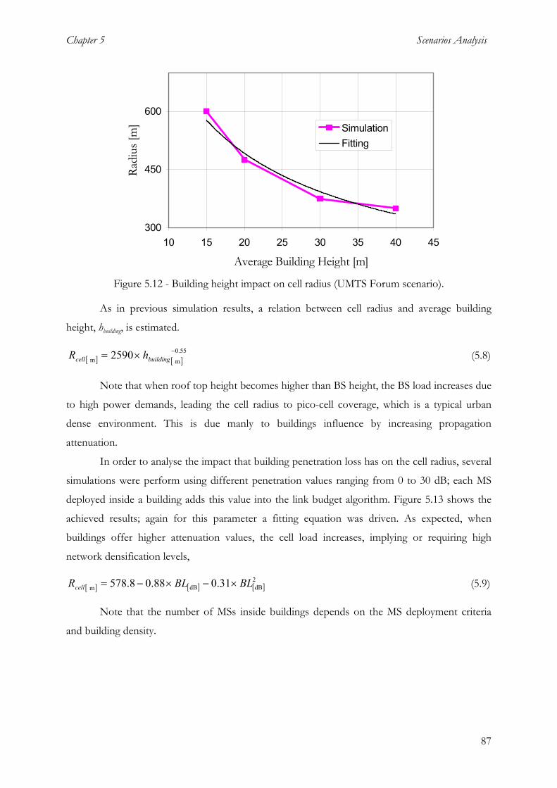
Chapter 5 Scenarios Analysis
300
450
600
10 15 20 25 30 35 40 45
Average Building Height [m]
Radi
us [m
] SimulationFitting
Figure 5.12 - Building height impact on cell radius (UMTS Forum scenario).
As in previous simulation results, a relation between cell radius and average building
height, hbuilding, is estimated.
[ ] [ ]55.0
m m 2590 −×= buildingcell hR (5.8)
Note that when roof top height becomes higher than BS height, the BS load increases due
to high power demands, leading the cell radius to pico-cell coverage, which is a typical urban
dense environment. This is due manly to buildings influence by increasing propagation
attenuation.
In order to analyse the impact that building penetration loss has on the cell radius, several
simulations were perform using different penetration values ranging from 0 to 30 dB; each MS
deployed inside a building adds this value into the link budget algorithm. Figure 5.13 shows the
achieved results; again for this parameter a fitting equation was driven. As expected, when
buildings offer higher attenuation values, the cell load increases, implying or requiring high
network densification levels,
[ ] [ ] [ ]2dBdBm 31.088.08.578 BLBLRcell ×−×−= (5.9)
Note that the number of MSs inside buildings depends on the MS deployment criteria
and building density.
87

Scenarios Analysis Chapter 5
250300350400450500550600
0 5 10 15 20 25 30
Building Penetration Loss [dB]
Radi
us [m
]Cell RadiusFitting
Figure 5.13 - Building penetration loss impact on cell radius.
5.4 Impact from Systems and Scenarios Characteristics
The impact that major configuration parameters have on the network behaviour is
presented in this section: for each parameter, some simulations were executed, assuming
parameters in Tables 5.2 and 5.3 as constants (UMTS Forum scenario).
One may start by analysing the impact that Soft Handover (SH) reservation channels
codes has on cell performance. To do this, several simulations with different SH channel codes
reservation percentage, ranging from 10 to 40 %, were carried out, Figure 5.14.
370
390
410
430
450
470
490
510
5 10 15 20 25 30 35 40 4Soft Handover Channels [%]
Rad
ius
[m]
5
Figure 5.14 - Impact of SH percentage on cell radius.
A trade off must be achieved, so that a BS can support handover and new connections
with reasonable success. Based on Figure 5.14, a reasonable value seems to be in the range from
20 to 30 %.
Another major network parameter is Eb/N0. In UMTS, each service has a minimum
Eb/N0 defined value, which means that the power control process aims to maintain this value at
the receiver when it interacts with the transmitter. One may say that for a high Eb/N0, (better
88

Chapter 5 Scenarios Analysis
signal quality) in UL and DL, transmitted power levels will be higher, increasing the BS load and
interference levels, therefore, the impact on cell radius regarding this effect must be analysed.
Figure 5.15 shows Eb/N0 plotted for “only voice service”; like in all others simulations, this result
depends on all other parameters, nevertheless, it is possible to observe Eb/N0 variation values,
and consequently the impact on the cell radius. As expected, for higher Eb/N0 targets the cell
radius decreases, in order to sustain its maximum allowed load.
425
475
525
575
625
675
0 2 4 6 8Only Voice Eb/No [dB]
Rad
ius
[m]
10
Simulation
Fitting
Figure 5.15 - Cell radius influence by Eb/N0 variation (only voice active).
It is possible to extract an analytical relation between Eb/N0 and the optimum cell radius.
In this example, one may conclude that for each Eb/N0 dB unit the cell radius decreases about 29
m.
[ ][ ]dB0
m 08.2939.719NE
R bcell ×−= (5.10)
All operators perform statistics concerning users behaviour, the service average
connection time being one among others that is computed. In order to understand the influence
on BS load due to this parameter, some simulations were carry out, Figure 5.16, with 60, 120 and
180 s of average connection time for the 128 kbps CS service, assuming voice with 60 s of
average call duration.
89

Scenarios Analysis Chapter 5
300350400450500550600650
60 120 180Aver. C. Time [s]
Rad
ius
[m]
SimulationFitting
Figure 5.16 - 128 kbps average connection duration influence in cell load/radius, plus voice.
Equation (5.11) is the analytical approximation that fits the curve and produces the lowest
error,
[ ] [ ] [2
s 128s 128m 5.625.112575 ATATRcell −+= ] (5.11)
where AT is the average connection time. Note that all other system parameters follow the
UMTS Forum scenario.
The blocking probability target has a major role on system performance in any kind of CS
based network, since when traffic increases in a given network, blocking probability increases. In
order to study the impact that the blocking threshold has on cell radius, several simulations were
performed (using only voice service) with different targets, ranging from 2 to 8 %.
540550560570580590600610620
0 2 4 6 8Blocking Probability [%]
Rad
ius
[m]
10
SimulationFitting
Figure 5.17 - Network influence as function of blocking percentage variation (only voice).
Figure 5.17 shows the optimum cell radius dependency on the blocking target. Like in all
previous results, an equation was derived:
[ ] [ ] [2%%m 2.15.2550 VBVBRcell +−= ] (5.12)
where VB is the voice blocking optimisation target.
90

Chapter 5 Scenarios Analysis
When resources are not available for PS communications, services get delayed. Some
services are more tolerant to delay than others, but if a maximum average delay for PS is
imposed, the cell radius will also converge to an optimum value. Like blocking probability, high
values for average delay will increase the cell radius. Figure 5.18 shows the simulations results,
where average simulation delay target were set from 2 to 8 s per packet.
525
575
625
675
725
775
825
0 2 4 6 8Delay [s/p]
Rad
ius
[m]
10
Cell RadiusFitting
Figure 5.18 - Network influence as function of average delay variation.
Again, an analytical approach was obtained, for the target delay, D.
[ ] [ ] [ ]2s/p s/p m 25.622575 DDRcell +×−= (5.13)
Call admission control may lead to a very complex world, but essentially it is an algorithm
that decides if a connection in the air interface is accepted or not. There are two indicators where
the simulation decides if a BS allows new connections or not. In order to perform a connection
the following conditions must be respected:
• Current DL load indicator must be below the threshold defined at the BS (default value is
70%);
• Channels codes must be available for the requesting service.
If one of these two indicators is not respected, blocking or delay will occur. Note that the
number of channel codes is constant, but DL load threshold is optional. In order to understand
how this influences the BS load, several simulations were perform for different DL load
thresholds. Figure 5.19 shows the results, where one can see that optimum threshold values are
achieved between 55 and 70 % of load, and also that values above 70 % lead the system to an
unstable power management, where increasing drop connections force a cell radius reduction.
91

Scenarios Analysis Chapter 5
490
510
530
550
570
590
610
50 55 60 65 70 75 80 85 90 95Load Thershold [%]
Rad
ius
[m]
Figure 5.19 - Network impact as function of load thresholds variation.
In order to understand how PS and CS services are related from the BS load point of
view, several scenarios were assumed and simulated, Table 5.4. For each switching type, different
values are distributed for each service.
Table 5.4 - Penetration distribution scenarios.
PS CS Penetration Distribution [%] HMM MMM SM HIMM SD S PS_45/CS_55 10 10 25 5 10 40 PS_40/CS_60 5 10 25 5 5 50 PS_35/CS_65 5 5 25 5 10 50
It is clear that results presented in Figure 5.20 directly depend on how individual service
penetration values are distributed: if high bit rate services have a huge penetration value, the cell
load will be quite different, so the cell radius is expected to decrease a bit.
440
450
460
470
480
490
500
510
PS_45/CS_55 PS_40/CS_60 PS_35/CS_65Penetration for PS and CS services
Rad
ius
[m]
Figure 5.20 - Penetration distribution impact on BS.
When a MS is active, power control is executed at 1500 Hz (slot level), which is the
defined standard value, nevertheless, it seams important to know the influence that this process
92

Chapter 5 Scenarios Analysis
has on network performance. In order to analyse this, simulations with quite different power
control frequency were performed. Figure 5.21 shows that higher power control frequencies
result in a higher optimisation level in the WCDMA interface, therefore, power (the shared
resource) will be managed more efficiently among to users, generating more capacity. This result
(capacity improvement due to power control) is already estimated in [OjPr98]. Fast power control
avoids the near-far effect, compensating a fading channel and reducing interference inside and
outside the cell.
410420430440450460470480490500510
0 200 400 600 800 1000 1200 1400 1600
Power Control Frequency
Radi
us [m
]
Figure 5.21 - Impact of power control frequency on cell radius.
5.5 Futuristic Scenario
It is hard to predict what the future will be from the service penetration point of view,
nevertheless, it is expect that some interactive services will have more users. Therefore, a new
scenario was set (futuristic scenario), where different service penetration values, compared to the
UMTS-Forum forecast, were simulated. This new scenario assumes PS services at 10 %, and CS
services at 20 and 60 % (the latter for voice). Basically, it assumes a strong growth in penetration
percentages, Table 5.5, related to UMTS-Forum scenario.
Table 5.5 - Penetration settings for each service (new scenario).
HIMM HMM MMM SD SM S
20% 10% 10% 20% 10% 60%
93
Simulation results are shown in Figure 5.22: cell radius and antenna height are shown as a
function of population density. Note that BS antenna height also presents some variation, which
is due to small modifications by the automatic optimisation process, because (as already explain in
previous chapters) cell radius convergence steps approximations where not enough to achieve the
network quality targets with precision. Note that for 12 500 pop/km2 case, the cell radius seems

Scenarios Analysis Chapter 5
to increase; again, this is due to the optimisation algorithm, which in this particular case, increases
the BS height. This means that network configuration process converges to a local optimum
point.
150
200
250
300
350
400
450
2500 5000 7500 10000 12500 15000 17500 20000Density [pop / km2]
Rad
ius
[m]
0
5
10
15
20
25
Hei
ght [
m]Cell Radius
BS HeightFitting (Cell Radius)
Figure 5.22 - Population density impact on cell radius with mixed services.
Comparing Figure 5.5 and Figure 5.22, the impact that higher penetration values has on
cell radius is clear, since cell radius gets smaller (small cells for all different populations densities).
One may conclude that, on average, cell radius decreases about 1.2 m for each extra 100 persons
per square kilometre inside the cell, assuming 4 operators and the network conditions mentioned
above.
The influence of one particular parameter on the cell radius may be estimated by running
several simulations using different values of this parameter; using these results, it is possible to
build an equation, which describes the impact on cell radius. This equation may be used as a
heuristic in analytical simulations, to evaluate the weight that an individual parameter has on the
optimum cell radius, and to estimate future scenarios.
94
Analysing all the previous parameters variation, one concludes that all of them have some
impact on the cell radius, therefore, on network capacity. This impact may be huge in some cases,
like high bit rate services, these services having a remarkable influence on the network capacity,
due to high power and channel codes consumption, increasing the number of BS per km2. When
the 2Mbps (HMM) service is used by an increasing number of users, the optimum cell radius
easily converges to around 100 m and below. Therefore, in order to maintain the network health,
some services usage (average connection time) may be “controlled” by the billing system.
However, there are some other parameters, which cannot be manipulated by the operator (i.e.

Chapter 5 Scenarios Analysis
95
building height, building walls penetration, etc); these parameters must be considered on the
simulation scenario as a way to consider their impact on the overall results.
For some particular parameters, the network performance is very sensitive; for example,
for the Eb/N0 voice target, the cell radius must be reduced about 30 m for each extra dB. Note
that this value was achieved with only voice active, and the Eb/N0 target for services with higher
bit rates will have more influence.
In this Chapter a reference scenario was simulated with the following characteristics: city
map and population density from Lisbon, services forecast from the UMTS-Forum, Eb/N0
targets from ETSI, and all other system parameters from literature. Besides performing an
analysis on parameters sensitivity, a futuristic scenario is proposed were data services usage is
increased, leading the BS density (network cost) to expected higher values. From the operator
point of view, one of the most interesting outputs of this analysis is the possibility to predict the
UMTS network financial cost based on main parameters (quality targets, coverage, services, users,
environment, UMTS, parameters, propagation, etc) specifications.


Chapter 6 Conclusions
97
6 Conclusions This thesis deals with radio planning and optimisation in UMTS networks. In order to
achieve this, one has to investigate four main areas: propagation, traffic, services and optimisation
techniques. UMTS planning puts many questions that have to be answered. Cell radius is a
fundamental network parameter, that responds to many of these questions, therefore, finding the
optimum cell radius is an important goal. Afterwards, coverage, cellular density, network cost and
many radio network configurations (as a function of a given scenario) are easily achieved.
Several cellular propagation models were examined. The COST 231 Walfish-Ikegami
model was selected, because it fits many UMTS constrains, being dedicated to micro-cellular
environments (urban scenario) and European cities. From the propagation point of view, urban
environmental aspects have a huge impact on network impact. For example, if the BS antenna
height is below buildings roof tops, or the MS is placed between high buildings, signals suffer
higher attenuation levels, which increase the radio link level for each user connection. This leads
the BS power level to its limits, causing power capacity problems, which can be solved only by
network densification (cell radius reduction); nevertheless, this is not a negative point, because
areas with high buildings usually have a high users density, needing high network densification.
Therefore, also the BS antenna height is optimised, aiming to enhance results accuracy
(particularly when it is tangential to building roof top), which, from the operator side, is very easy
to adjust.
Traffic generation in the simulation is a key element in planning, because it is mainly
based on this that all other parameters are achieved. Traffic depends on user’s profile, which is
generated as a function of services usage, defined by penetration, bit rate, time constrains, average
connection time, location, etc. Based on this, traffic source models are used to simulate user’s
traffic in the air interface: Poisson distribution to characterise connection arrival process, ON-
OFF model for PS and data transfer based on CS, and exponential distribution to model the
typical voice call duration.
When propagation, traffic and services are being simulated, a feedback process, based on
quality network indicators, performs adequate changes on cell radius or BS antenna height. This
process is repeated until quality targets are accomplished, producing an optimum cell radius, for a
given scenario. The UMTS Forum scenario is used as reference.
High codes consumption is made mainly by high bit rate services with low spreading
factors. Furthermore, extra codes are needed for MS in soft handover. The use of a single code
per user implies orthogonality among the different services provided by the cell, which exists only

Conclusions Chapter 6
98
in theory; in reality, the multipath environment disrupts the orthogonality among them, causing
interference. In this work, only one cell is simulated, inter-cell interference being extrapolated
from intra-cell one. Therefore, results about inter-cell interference present some error,
nevertheless, intra-cell one is expected to be the most problematic, due to short distance reasons.
Coverage in UMTS is quite a complex issue, because each connection (service) may use
different bit rates, which means different spreading factor and processing gain. High bit rates will
certainly have some gaps in coverage, mostly probably outside hot-spot areas, where the network
density is lower. In order to guaranty high capacity and coverage, the network cost will be
necessarily increased, because the number of BSs density has to be higher.
Indoors coverage in this work has a simplistic approach: any user located in a building,
suffers additional loss (average building penetration value) in the link budget calculations. A
higher penetration loss produces higher loads into the BS, due to power control. Therefore,
accurate information about building penetration values will increase the simulation precision.
In order to maintain coverage, capacity, services within network quality indicators, in a
growing population density scenario, the cellular network density (resources per area) must be
increased to sustain an inherent growing traffic. Hence, the generated traffic is a very important
issue, i.e., if users use only the voice service the BSs density will be lower than in a network where
users use high data rate services (multimedia ones). One may conclude that network planning is
very sensitive to user’s generated traffic, which implies a very careful radio network planning,
aiming to achieve the optimum network configuration.
The simulation tool developed in this thesis has an “MS and BS oriented design”,
meaning that each MS and BS has its own state machine, each state being responsible to initiate
independent services connections, based on traffic source models and services forecasts. This
approach is good to simulate reality and takes advantage from the intrinsic object oriented
programming language used (C++). When information concerning user/services (traffic),
propagation, environment (map/buildings), equipment (i.e. antennas) and simulation parameters
(i.e. quality targets) are introduced, the simulation engine may start. The propagation model and
the link budget algorithm estimate power and interference received by MSs, in parallel the BS
runs simple RRM algorithms. If traffic generated by services does not match the network
capacity, some changes are perform in the network, aiming to a get an optimal configuration.
One simulation is composed of many parameters defining the system and the scenario, all
of them having influence on results. In order to analyse the planning sensitivity to each
particularly parameter, a set of simulations was carried out, varying only one parameter in each
simulation. Parameters like population density (number of users), service penetration, average
service connection time, bit rate, Eb/N0 target for each service, urban environment, connection

Chapter 6 Conclusions
99
rate, BS load threshold, antenna pattern, additional attenuations, fading and interference margins,
soft handover, orthogonality level, blocking probability and delay targets, were accounted for; the
weight that each parameter has is measured as a function of the optimum cell radius result. In
many cases, the cell radius tendency is naturally expected, nevertheless, an important knowledge
is learned: the order of magnitude or impact that a parameter has on the cellular structure.
One may conclude, for example, that an operator with only voice service active, may
reduce on average about 50 m on the cell radius, for each 800 customers per km2 (linear
decrease). In the case of all active services, the UMTS Forum scenario has about the same
relationship, but with an initial offset on radius, around 150 m less than the previous case, which
translates the multimedia impact. Based on the forecast from the UMTS Forum, one may
conclude that for each year, the cell radius should decreased about 23 m, this seams to be a
neglectable value, considering that operators are constantly performing network upgrade, and
optimising it in function of growing traffic.
Main services were also individually analysed, 384 kbps with a growing penetration added
to voice presenting an exponential curve in the optimum cell radius. Also the 2000 kbps service
presents the same tendency. This effect is mainly due to the high bit rate service impact on the
network (low service penetration), since for a growing that when penetration the cell radius
becomes smaller, nearly to the indoor case, for 2000 kbps.
The BS load threshold is a quite sensitive parameter. If it is set to high values, the BS
allows new connections, even with a high load, and the BS, reaches the limit very fast due to
power control, therefore, also very fast, many connections will be dropped, essentially due to
power restrictions. This effect was detected in simulations, when this parameter was set above
70%, and to prevent this effect, values between 50% and 60% are recommended.
For each service, a different Eb/N0 minimum quality value is defined and imposed, which
has a huge impact on cell radius: higher values introduces higher power needs in the radio links,
hence the optimum cell radius must be decreased to avoid the BS power limit and the network
collapse. Therefore, a trade-off between quality parameters and network cost must be found, in
order to minimise the impact that these parameters have on the network.
In UMTS system simulation level, it is virtually impossible to create a highly accurate
simulator, due to the huge number of environments and system aspects that need to be modelled
and simulated. It is obvious that this thesis cannot addresses in a realistic way all the issues that
have impact on radio network planning, optimisation, and simulation, thus, many topics are left
for further work which include several environmental and system mechanisms that lead to a more
realistic simulation.

Conclusions Chapter 6
100
Adding terrain information to the simulation, like digital terrain height and classification
databases makes it possible to implement accurate radio propagation models. Also building
information, like construction type and height, is very important in urban environments.
User distribution density and mobility modelling has also a huge importance in mobile
communications. GSM existing knowledge may be a good starting point. Mobility modelling
introduces also a higher level of realism in simulations, because it enables to address many
problems, e.g., traffic jams, highways traffic, handover statistics, and drop connections
(pedestrian and vehicular networks analysis). These characteristics make possible the
implementation of a better network optimisation process concerning other issues besides radio
planning, i.e., handover algorithms.
Soft, softer and hard handover implementation is also suggested. Hierarchical Cell
Structure is also very importance in network planning, because a UMTS operator may use
overlaid macro-, micro- and pico-cells in order to increase network capacity or to provide special
services coverage. Other system aspects, like radio resource management (RNCs simulation)
optimisation algorithms, may be integrated into simulation, where many network configuration
options may be optimised.
UMTS may be seen as a “mobile multi-service platform”, which brings many new traffic
concepts that need to be investigated. For example, traffic source models, related to multimedia
services in a CDMA radio interface, must be included in simulations. Therefore traffic source
models that produce accurate multi service simulation, like voice, WWW based services (HTTP,
e-mail, FTP, UDP, VoIP, etc), data (PS and CS), video, etc., have to be implemented, in order to
introduce more realism to system simulation and consequently planning accuracy.
Initially UMTS deployment will be based on GSM location sites, due to economical and
already tested propagation reasons; nevertheless, new sites will be required, in order to offer
capacity to incoming users, therefore, it is also suggested for future work to investigate an
algorithm that optimises BS deployment location and configuration.

Annex A UMTS Characteristics
Annex A - UMTS Characteristics Figure A.1 (MS UL transmitter) shows the general spreading scheme in the case where
several UL DPDCHs are used.
IΣ
j
cd,1 βd
Sdpch,n
I+jQ
DPDCH1
Q
cd,3 βd
DPDCH3
cd,5 βd
DPDCH5
cd,2 βd
DPDCH2
cd,4 βd
DPDCH4
cd,6 βd
DPDCH6
cc βc
DPCCH
Σ
S
Figure A.1 - Spreading for uplink DPCCH and DPDCHs (extracted from [3GPP00d]).
Each different DPDCHn carry different types of services multiplexed by different
channelisation codes (Cd,n). Each channel has their own independent power level, which are
controlled by different power regulators (βd).
The generation method for the channelisation code is defined [3GPP00d] as follows:
1Cch,1,0 = ,
−
=
−
=
1111
0,1,
0,1,
0,1,
0,1,
1,2,
0,2,
ch
ch
ch
ch
ch
ch
CC
CC
CC
101

UMTS Characteristics Annex A
( )
( )
( )
( )
( ) ( )
( ) ( )
−
−
−
=
−−
−−
−++
−++
+
+
+
+
12,2,12,2,
12,2,12,2,
1,2,1,2,
1,2,1,2,
0,2,0,2,
0,2,0,2,
112,12,
212,12,
3,12,
2,12,
1,12,
0,12,
:::
nnchnnch
nnchnnch
nchnch
nchnch
nchnch
nchnch
nnch
nnch
nch
nch
nch
nch
CCCC
CCCCCC
CC
CC
CCCC
The leftmost value in each channelisation code word corresponds to the chip transmitted
first in time. In [3GPP00d] the scrambling codes are specified.
Figure A.2 and Figure A.3 illustrates the principle of RAKE receiver. After transmission,
the signal passes through a multipath channel, which is modelled by several delayed blocks τ1, τ2
and τ3, and afterwards attenuated by a1, a2 and a3 lines (signals which are reflected are delayed and
attenuated in a multipath channel), corresponding to each relevant propagation path. Because the
MSs is in "permanent" movement the delay and attenuation factors are also dynamic, so the
RAKE receiver requires a constant measurement on the tapped delay line profile and to reallocate
RAKE fingers.
Data
CodeGenerator
X Modulator
3τ
2τ
1a
2a
3a
1τ
+
Multipath Channel Model
Figure A.2 - The transmitter and the Multipath Channel Model (adapted from [OjPr98]).
Note that the number of “fingers” in the RAKE receiver will be typically 3 or 4, because
higher numbers will increase the receiver complexity, and do not bring too much gain (higher
signal components are 3 or 4).
102

Annex A UMTS Characteristics
1a
2a
3a
+
Rake Receiver
Demodulator
X
X
X
( )3τ−tCode
( )1τ−tCode
( )2τ−tCode
Figure A.3 - RAKE receiver architecture model (adapted from [OjPr98]).
103

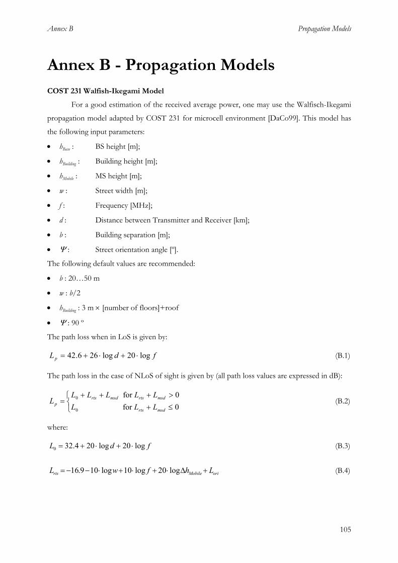
Annex B Propagation Models
Annex B - Propagation Models COST 231 Walfish-Ikegami Model
For a good estimation of the received average power, one may use the Walfisch-Ikegami
propagation model adapted by COST 231 for microcell environment [DaCo99]. This model has
the following input parameters:
• hBase : BS height [m];
• hBuilding : Building height [m];
• hMobile : MS height [m];
• w : Street width [m];
• f : Frequency [MHz];
• d : Distance between Transmitter and Receiver [km];
• b : Building separation [m];
• Ψ : Street orientation angle [º].
The following default values are recommended:
• b : 20…50 m
• w : b/2
• hBuilding : 3 m × [number of floors]+roof
• Ψ : 90 º
The path loss when in LoS is given by:
fdLp log20log266.42 ⋅+⋅+= (B.1)
The path loss in the case of NLoS of sight is given by (all path loss values are expressed in dB):
≤+>+++
=0for 0for
0
0
msdrts
msdrtsmsdrtsp LLL
LLLLLL (B.2)
where:
fdL log20log204.320 ⋅+⋅+= (B.3)
oriMobilerts LhfwL +∆⋅+⋅+⋅−−= log20log10log109.16 (B.4)
105

Propagation Models Annex B
( )( )
≤Ψ≤−Ψ⋅+<Ψ≤−Ψ⋅+
<Ψ≤Ψ⋅+−=
º90º55for 55114.00.4º55º53for 35075.05.2
º35º0for 34.010
oriL (B.5)
bfKdKKLL fdabshmsd log9loglog ⋅−⋅+⋅++= (B.6)
where:
( )
for 0for 1log18
≤
>∆+⋅−=
BuildingBase
BuildingBaseBasebsh hh
hhhL (B.7)
BuildingBaseBase hhh −=∆ (B.8)
≤<⋅∆⋅−
≤≥∆⋅−
>
=
BuildingBaseBase
BuildingBaseBase
BuildingBase
a
hhddh
hhdh
hh
K
e km 5.0for 5.08.054
e km 5.0for 8.054
for 54
(B.9)
≤∆⋅−
>=
BuildingBaseBuildingBase
BuildingBased hhhh
hhK
for 1518for 81
(B.10)
( )
( )
−⋅+−
−⋅+−
=
centresan metropolitfor 1925514árvores de densidade
density treemoderate with centres suburban and cities size mediumfor 1925704
f.
f.
K f (B.11)
L0 is the free space attenuation, Lrts is "roof-to-street diffraction and scatter loss", Lori is
the attenuation caused by main street orientation with respect to the direct radio path and Lmsd is
the "multi-screen diffraction loss". The output parameter of the model is LP in dB.
Some parameters have a validity range, Table B.1.
106

Annex B Propagation Models
Table B.1 - Valid parameters range.
Frequency 800…2000 MHz
Distance NLoS 0.02…5 km
Distance LoS 0.02…0.2 km
BS antenna height 4…50 m
MS antenna height 1…3 m
3GPP Propagation Models
For each environment, a different formulation is used to evaluate the path loss. An
important parameter to be defined is the Minimum Coupling Loss (MCL), i.e., the minimum
distance loss including antenna gain measured between antenna connectors; in [3GPP00a] the
MCL of 70 dB is assumed for the macro-cellular environment and 53 dB for the micro-cellular
one.
With the above definition, the received power in DL or UL can be expressed for the
macro-cellular environment as:
, MCL) - G- G (L - P P RxTxp,macroTxRx max= (B.12)
and for the micro-cellular as:
, MCL) - G- G (L - P P RxTxp,microTxRx max= (B.13)
where PRx is the received signal power, PTx is the transmitted signal power, GTx is the transmitter
antenna gain, GRx is the receiver antenna gain. Lp,macro and Lp,micro are the output of the propagation
model. It is assumed an antenna gain of 11 dBi (including cable losses) in the BS and 0 dBi in the
MS.
The macro-cell propagation model proposed by the 3GPP is applicable for test scenarios
in urban and suburban areas outside the urban core, where the buildings are of nearly uniform
height. The micro-cell model also adopted one proposed in [ETSI98]. This model is to be used
for spectrum efficiency evaluations in urban environments, through a Manhattan-like structure, in
order to properly evaluate the performance in micro-cell situations that will be common in
European cities at the time of UMTS deployment. The proposed model is a recursive one, which
calculates path loss as a sum of LoS and NLoS segments. The shortest path along streets between
the BS and the MS has to be found within the Manhattan environment.
The macro-cell model is:
80)(log21)(log18)(log)1041(40 1010103%50
, +⋅+⋅−⋅⋅⋅−⋅= − fDdDL hbhbmacrop (B.14)
107

Propagation Models Annex B
where:
• d is the distance between BS and MS [km];
• f is the carrier frequency [MHz] (default 2000);
• Dhb is the BS antenna height, measured from the average rooftop level, [m] (default, 15 m);
• is the average path loss [dB]. %50,macropL
After is calculated, log-normally distributed shadowing, LogF, with standard
deviation of 10 dB should be added, so that the resulting path loss is the following:
%50,macropL
LogFLL macropmacrop += %50,, (B.15)
The following constrains: applies:
1. shall in no circumstances be less than free space loss. This model is valid for NLoS
case only and describes the worse case propagation.
%50,macropL
2. The model is valid for a range of Dhb from 0 to 50 m.
3. This model is designed mainly for distances from few hundred meters to kilometres, and it is
not very accurate for short distances.
The micro-cell model has the path loss given by:
λπ n
micropd
L4
log20 10%50, ⋅= (B.16)
where:
• dn is the "illusory" distance;
• λ is the wavelength;
• n is the number of straight street segments between BS and MS (along the shortest path).
The illusory distance is the sum of these street segments, and can be obtained by
recursively using expressions kn = kn-1+dn-1c and dn = kn sn-1 +dn-1, where c is a function of the angle
of the street crossing. For a 90º street crossing, c should be set to 0.5. Further, sn-1 is the length in
meters of the last segment. The initial values are set 1 for k0 and 0 for d0. The illusory distance is
obtained as the final dn when the last segment has been added.
The model is extended to cover the micro-cell dual slope behaviour, by modifying the
expression to:
⋅⋅= ∑
=−
n
jj
nmicrop sD
dL
1110
%50,
4log20
λπ
(B.17)
where:
108

Annex B Propagation Models
≤>
=br
brbr
xdxdxd
dD,1
,/)( (B.18)
being d the distance from the transmitter to the receiver.
Before the break point xbr, the slope is 2, after the break point it increases to 4; the break
point xbr is set to 300 m. To take effects of propagation going above rooftops into account, it is
also needed to calculate the path loss according to the shortest geographical distance. This is done
by using the commonly known COST Walfish-Ikegami Model, and with antennas below
rooftops:
( )20log4524%50, +⋅+= dL microp (B.19)
where d is the shortest physical geographical distance from the transmitter to the receiver in [m].
The final path loss value is the minimum between the path loss value from the
propagation through streets and the path loss based on the shortest geographical distance, plus
the log-normally distributed shadowing, LogF, (with standard deviation of 10 dB).
( ) LogFLLL macropmicropmicrop += ,%50,, ,min (B.20)
COST 231-Hata-Model
COST 231 has extended Hata's model to the frequency band [1500, 2000] MHz by
analysing Okumura's propagation curves in the upper frequency band. This combination is called
"COST-Hata-Model" described in [DaCo99].
( ) ( ) ( ) ( )( ) ( ) mBaseMobileBaseb CdhhahfL +⋅⋅−+−⋅−⋅+= loglog55.69.44log82.13log9.333.46 (B.21)
where
( ) ( )( ) ( )( )8.0log56.17.0log1.1 −⋅−⋅−⋅= fhfha MobileMobile (B.22)
Cm being 0 dB for medium sized city and suburban centres with medium tree density, and 3 dB
for metropolitan centres.
The COST-Hata-Model is restricted to the following range of parameters:
• f : 1500 ... 2000 MHz
• hBase : 30 ... 200 m
• hMobile : 1 ... 10 m
• d : 1 ... 20 km
The application of the COST-Hata-Model is restricted to large and small macro-cells, i. e.,
BS antenna heights above roof-top levels adjacent to it. Hata's formula and its modification must
not be used for micro-cells. 109


References
111
References [3GPP00a] 3GPP, RF System Scenarios, 3GPP Technical Specification Group Radio Access
Networks, Report No. 25.942 version 2.1.3, Mar. 2000 (http://www.3gpp.org).
[3GPP00b] 3GPP, UE Radio Transmission and Reception (FDD), 3GPP Technical Specification
Group Services and Systems Aspects, Report No 25.101 version 3.0.1, Mar. 2000
(http://www.3gpp.org).
[3GPP00c] 3GPP, Physical Channels and Mapping of Transport Channels on to Physical Channels
(FDD), 3GPP Technical Specification Group Radio Access Network, Report No
25.211 version 3.2.0, Mar. 2000 (http://www.3gpp.org).
[3GPP00d] 3GPP, Spreading and Modulation (FDD), 3GPP Technical Specification Group
Radio Access Network, Report No. 25.213 version 3.2.0, Mar. 2000
(http://www.3gpp.org).
[3GPP00e] 3GPP, UE Radio Transmission and Reception (TDD), 3GPP Technical Specification
Group Radio Access Network, Report No. 25.102 version 3.2.0, Mar. 2000
(http://www.3gpp.org).
[3GPP00f] 3GPP, UE Radio Transmission and Reception (FDD), 3GPP Technical Specification
Group Radio Access Network, Report No. 25.101 version 3.2.0, Mar. 2000
(http://www.3gpp.org).
[3GPP00g] 3GPP, Physical Channels and Mapping of Transport Channels onto Physical Channels
(TDD), 3GPP Technical Specification Group Radio Access Network, Report No.
25.221 version 3.2.0, Mar. 2000 (http://www.3gpp.org).
[CMLi01] Câmara Municipal de Lisboa (Lisbon Town Hall), Direcção de Planeamento e
Gestão Urbanística; 2001.
[DaCo99] Damosso, E. and Correia, L.M., Digital Mobile Radio Towards Future Generation
Systems, COST 231 Final Report, Brussels, Belgium, 1999.
References
112
[DaEr00] Damme, E., “UMTS auctions in Europe”, Erasmus University Rotterdam, Medium
Econometrische Toepassingen, Netherlands, Jan. 2001, pp 4-8.
[Dahl98] Dahlman, E., Gudmundson, B., Nilsson, M. and Skold, A. "UMTS/IMT-2000
Based on Wideband CDMA", IEEE Communications Magazine, Vol. 36, No. 9, Sep.
1998, pp. 70-80.
[ETSI00] ETSI, SMG2, Self-evaluation report on Radio Transmission Technology for UMTS
Terrestrial Radio Access, Sophia-Antipolis, France, Sep. 1998.
[ETSI98] ETSI, Selection procedures for the choice of radio transmission technologies of the UMTS, TR
101 112 v3.2.0 , France, Apr. 1998.
[Garcia00] Garcia, M. A. C., Analysis of Multi-Service Traffic in UMTS FDD mode Networks, IST,
Technical University of Lisbon, Portugal, May 2000.
[Hata80] Hata, M., "Empirical Formula for Propagation Loss in Land Mobile Radio
Services", IEEE Trans. Veh. Technol., Vol. VT-29, No. 3, Aug. 1980, pp. 317-325.
[HaTo00] Holma, H. and Toskala, A., WCDMA for UMTS, John Wiley, Chichester, UK,
2000.
[Héra02] Hérault, L., ASILUM - Advanced Signal Processing Schemes for Link Capacity Increase in
UMTS, Final Report, IST Central Office, Brussels, Belgium, Mar. 2002.
[ICPo01] Instituto Comunicações de Portugal, 2001 (http://www.icp.pt).
[IkYU84] Ikegami, F., Yoshida, S. and Umehira, M., "Propagation factors controlling mean
field strength on urban streets," IEEE Trans. on Antennas and Propagation, Vol. 32,
No. 8, Aug. 1984, pp. 822-829.
[JeMo01] Jehiel, P. and Moldovanu, B., The European UMTS/IMT-2000 License Auctions,
Centre d’Ensegnement et de Recherche en Analyse Socio-Economique, Paris,
France, Jan. 2001. (http://www.enpc.fr/ceras/)
References
113
[KNLA01] Kaaranen, H., Naghian, S., Laitinen, L., Ahtiainen, A. and Niemi V., UMTS
Networks: Architecture, Mobility and Services, John Wiley, Chichester, UK, 2001.
[MePi99] Menolascino, R. and Pizarroso, M., STORMS - Software Tools for the Optimisation of
Resources in Mobile Systems, Final Report, ACTS Central Office, Brussels, Belgium,
Apr. 1999.
[MOME01] MOMENTUM, Models and Simulation for Network Planning and Control for UMTS,
IST-MOMENTUM Project Technical Annex, KPN Research Leidschendam, The
Netherlands, May 2001.
[OjPr98] Ojanpera, T. and Prasad, R., Wideband CDMA for Third Generation Mobile
Communications, Artech House, London, UK, 1998.
[OOKF68] Okumura, Y., Ohmori, E., Kawano, T. and Fukuda,K., "Field Strength and Its
Variability in VHF and UHF Land-Mobile Radio Service", Rev. Elec. Commun.
Lab., Vol. 16, Sep.-Oct. 1968, pp. 825-873.
[Rapp96] Rappaport, T. S., Wireless Communications, Prentice Hall, London, UK, 1996.
[UMTS01] UMTS Forum, The UMTS Third Generation Market Phase II-Structuring The Service
Revenue Opportunities, Report No. 13, London, UK, Apr. 2001.
[UMTS98a] UMTS Forum, Minimum spectrum demand per public terrestrial UMTS operator in the
initial phase, Report No. 5, London, UK, Sep. 1998.
[UMTS98b] UMTS Forum, UMTS/IMT-2000 Spectrum, Report No. 6, London, UK, Dec.
1998.
[UMTS99] UMTS Forum, The Future Mobile Market Global trends and developments with a focus on
Western Europe, Report No. 8, London, UK, Mar. 1999.

References
114
[WaBe88] Walfisch, J. and Bertoni, H. L., "A theoretical model of UHF propagation in
urban environments," IEEE Trans. on Antennas and Propagation, Vol. 36, No. 12,
Dec. 1988, pp. 1788-1796.
[Yaco93] Yacoub, M. D., Foundations of Mobile Radio Engineering, CRC Press, Boca Raton,
Florida, USA, 1993.


