

i
OPTIONS EXPLAINED SIMPLY
THE FUNDAMENTAL PRINCIPLES COURSE

ii

OPTIONS EXPLAINED SIMPLY
THE FUNDAMENTAL PRINCIPLES COURSE
BALBINDER CHAGGER
Balbinder Chagger
2016

Options Explained Simply: The Fundamental Principles Course
This first edition published in 2016 by Balbinder Chagger
Copyright © 2016 by Balbinder Chagger
All rights reserved
The right of Balbinder Chagger to be identified as author of this work has been
asserted in accordance with the Copyright, Designs, and Patents Act 1988
All rights reserved. This book or any portion thereof may not be reproduced or used
in any manner whatsoever without the express written permission of the publisher
except for the use of brief quotations in a book review or scholarly journal.
Every reasonable effort has been made to ensure the information contained in this
publication is accurate at the time of going to press, and the publisher and the author
cannot accept responsibility for any errors or omissions, however caused. No
responsibility for loss or damage occasioned to any person or organisation acting, or
refraining from action, as a result of the material in this publication can be accepted
by the publisher or the author.
Cover designs, typesetting, illustrations, and graphics by Balbinder Chagger
www.OptionsExplainedSimply.com
First Printing: 2016
ISBN-13: 978-1-537-09092-4

DEDICATION
Sumitran & Harbhajan


CONTENTS
ABOUT THE AUTHOR .......................................................................... xiii
PREFACE ..................................................................................................... xv
INTRODUCTION ......................................................................................... 1
Part 1 SPOT & OTHER FUNDAMENTALS ....................................... 3
Lesson 1 SPOT ........................................................................................... 5
1.1 Spot Trades ................................................................................ 5
Lesson 2 POSITION TYPES ................................................................... 9
2.1 Expressing Ownership of Assets..................................... 10
2.2 Short Position Types ........................................................... 12
Lesson 3 SPOTS RISKS......................................................................... 17
3.1 Risk Source .............................................................................. 17
3.2 Delta: Spot Price Risk Measure ....................................... 18
3.3 Delta of a Long Stock Position ......................................... 21
3.4 Delta of a Short Stock Position ........................................ 25
Lesson 4 ARBITRAGE .......................................................................... 29
4.1 Deterministic Arbitrage ..................................................... 29
4.2 Statistical Arbitrage ............................................................. 32

viii
Lesson 5 RATIONALITY ...................................................................... 37
Lesson 6 TIME VALUE OF MONEY .................................................. 41
6.1 Future Value (FV) .................................................................. 41
6.2 Meaning of Future Value .................................................... 43
6.3 Discrete & Continuous Compounding Methods ........ 44
6.4 Simple Compounding .......................................................... 47
6.5 Continuous vs Discrete vs Simple ................................... 49
6.6 Present Value (PV) ................................................................ 50
Part 2 FORWARDS ................................................................................. 53
Lesson 7 FORWARDS ........................................................................... 55
7.1 Forward Trades ..................................................................... 55
7.2 Managing Risk with Forwards ......................................... 57
7.3 Forward’s Payoff Profiles ................................................... 57
Lesson 8 VALUING FORWARDS ....................................................... 61
8.1 Determining the Forward Price ....................................... 61
8.2 Meaning of Forward Price ................................................. 65
8.3 Spot Price & Forward Price Relationship .................... 66
8.4 Valuing Forward Contracts ............................................... 67
8.5 Importance of Forwards ..................................................... 68
Lesson 9 FORWARDS RISKS OVERVIEW ...................................... 69
9.1 Risk Sources ............................................................................ 69
Lesson 10 DELTA OF FORWARDS ................................................... 73
10.1 Spot Price & Forward Price Relationship .................... 73
10.2 Delta of a Forward ................................................................ 74
Lesson 11 RHO OF FORWARDS ........................................................ 79
11.1 Interest Rate & Forward Price Relationship .............. 79
11.2 Rho: Interest Rate Risk Measure ..................................... 80
11.3 Rho of a Forward ................................................................... 81
Lesson 12 THETA OF FORWARDS .................................................. 85
12.1 Time & Forward Price Relationship .............................. 85
12.2 Theta: Time to Expiry Risk Measure.............................. 86
12.3 Theta of a Forward ............................................................... 87
Lesson 13 DIVIDEND RISK OF FORWARDS ................................. 91
13.1 Dividends & Forward Price Relationship .................... 91
ix
13.2 Dividend Risk ......................................................................... 92
13.3 Dividend Risk of a Forward .............................................. 93
Part 3 FUTURES ..................................................................................... 97
Lesson 14 FUTURES ............................................................................. 99
14.1 Future Trades vs Forward Trades ................................. 99
14.2 Physical & Cash Settlements .......................................... 103
14.3 Daily Margining ................................................................... 104
14.4 Valuing Future Contracts ................................................. 105
Lesson 15 FUTURES RISKS OVERVIEW ..................................... 107
15.1 Risk Sources .......................................................................... 107
Lesson 16 DELTA OF FUTURES ..................................................... 109
16.1 Delta of a Future .................................................................. 109
Lesson 17 RHO OF FUTURES .......................................................... 113
17.1 Rho of a Future .................................................................... 113
Lesson 18 THETA OF FUTURES..................................................... 117
18.1 Theta of a Future ................................................................. 117
Lesson 19 DIVIDEND RISK OF FUTURES ................................... 121
19.1 Dividend Risk of a Future ................................................ 121
Part 4 OPTIONS .................................................................................... 125
Lesson 20 OPTIONS ............................................................................ 127
20.1 The Binding Nature of Forward Contracts ............... 127
20.2 Option Contracts ................................................................. 131
20.3 Call Options ........................................................................... 134
20.4 Put Options ....................................................................... 136
Lesson 21 VALUING EUROPEAN OPTIONS ............................... 141
21.1 ITM Value ............................................................................... 141
21.2 Chance Value ........................................................................ 145
21.3 Components of an Option’s Value ................................ 146
Lesson 22 VOLATILITY ..................................................................... 149
22.1 Spot Price Volatility ........................................................... 150
22.2 Time to Expiry ..................................................................... 152
22.3 Probability Distributions ................................................. 153
22.4 Discrete Probability Distributions ............................... 153

x
22.5 Continuous Probability Distributions ........................ 156
Lesson 23 ITM VALUE OF OPTIONS ............................................ 163
23.1 ITM Value of Call Options ................................................ 164
23.2 ITM Value of Put Options ................................................ 166
Lesson 24 CHANCE VALUE OF OPTIONS ................................... 169
24.1 Chance Value of ITM Options ......................................... 170
24.2 Chance Value of OTM Options ....................................... 174
Lesson 25 OPTION VALUES ............................................................ 179
25.1 ITM Call Options ................................................................. 179
25.2 OTM Call Options ................................................................ 184
25.3 ITM Put Options .................................................................. 189
25.4 OTM Put Options ................................................................ 192
Lesson 26 PUT-CALL PARITY ........................................................ 197
26.1 Synthetic Forwards ........................................................... 197
26.2 Value of a Synthetic Forward ........................................ 198
26.3 Put-Call Parity ...................................................................... 200
26.4 Put-Call Parity Violation .................................................. 201
Lesson 27 LEVERAGE ........................................................................ 203
27.1 Leverage ................................................................................ 203
27.2 Increasing Exposure.......................................................... 204
27.3 Reducing Investment ........................................................ 206
Lesson 28 OPTIONS RISKS OVERVIEW ...................................... 209
28.1 Risk Sources ......................................................................... 209
Lesson 29 DELTA OF OPTIONS ..................................................... 213
29.1 Delta of Call Options .......................................................... 213
28.2 Delta of Put Options .......................................................... 222
Lesson 30 VEGA OF OPTIONS ........................................................ 233
30.1 Vega: Volatility Risk Measure ........................................ 233
30.2 Vega of Call Options........................................................... 234
30.3 Vega of Put Options ........................................................... 238
Lesson 31 RHO OF OPTIONS .......................................................... 243
31.1 Rho of Call Options ............................................................ 243
31.2 Rho of Put Options ............................................................. 247

xi
Lesson 32 THETA OF OPTIONS ..................................................... 253
32.1 Time’s affect on Option Values ...................................... 253
32.2 Theta of Call Options ......................................................... 254
32.3 Theta of Put Options .......................................................... 261
Lesson 33 DIVIDEND RISK OF OPTIONS.................................... 269
33.1 Dividends and Basis ........................................................... 269
33.2 Call Options ........................................................................... 270
33.3 Put Options ............................................................................ 276
Lesson 34 VALUING AMERICAN OPTION .................................. 283
34.1 Early Exercise ....................................................................... 283
34.2 American Call Options with Dividends ...................... 284
34.3 American Call Options without Dividends ................ 286
34.4 American Put Options ....................................................... 288
EPILOGUE ................................................................................................ 291


xiii
ABOUT THE AUTHOR
Balbinder Chagger is a Chartered Accountant of the ICAEW. He has
an MBA from Cass Business School, London, and a BSc in Computer
Engineering from City, University of London. He also has formally
recognised teaching skills, developed while acquiring a PGCE in
Secondary School Mathematics at the UCL Institute of Education,
London, and working as a Mathematics Teacher.
Balbinder has a rigorous understanding of Options, consolidated over
13 years of professional practice in the Market Risk and Product
Control functions of global investment banks. His ability to teach
Options simply enables you to understand them easily.


xv
PREFACE
Welcome to Options Explained Simply: The Fundamental Principles
Course.
My objective is to explain Options simply enough to enable a wide
audience to understand them easily.
Balbinder Chagger
July 2016


BALBINDER CHAGGER
1
INTRODUCTION
An Option is a Derivative, which is a contract whose value depends
on (i.e., is derived from) the value of an Underlying Asset. For
example, a Microsoft share is an Asset and a Microsoft Option is a
contract whose value depends on the market price of the Microsoft
share. Options can be based on any Underlying Asset, not exclusively
on Stocks.
This course is an introduction to Options and is suitable for complete
novices to finance; prior specialised financial knowledge is not a pre-
requisite. It is a lesson-by-lesson taught course that will give you an
intuitive and sound understanding of what Options are, how they are
valued, and how they behave. It will give you the knowledge and the
confidence necessary to analyse Options intelligently, and set you up
well for further Options study, should you wish to pursue any.
The level of mathematics usually associated with Options is advanced
and sophisticated. It is beyond the level that most people choose to
pursue an education in mathematics to. An advanced layer of
mathematics makes Options appear incomprehensible and
intimidating to most people. To avoid that, and to allow a wide
audience to understand, this course is taught with simplified

OPTIONS EXPLAINED SIMPLY: THE FUNDAMENTAL PRINCIPLES COURSE
2
mathematics. All that is required is confidence with arithmetic, basic
algebraic expressions, averages, simple interest, and reading graphs.
The following steps have also been taken in order to promote
understanding:
The subject matter is often taught with reference to familiar,
real-life scenarios.
The amount of detail is simplified to keep the subject matter
clear and unclouded by unnecessary layers of complexity.
Visualisation, an important and powerful means for learning
for most people, is extensively utilised. Often, the written
explanations given are complimented with graphical
illustrations in order to clarify the subject matter more than
words alone do. The calculations presented are visually
transparent in that every key step in them is clearly shown.
Coloured text is used to emphasise and/or clarify key points,
as is done in this introduction.
To understand Options, you firstly need to understand Forwards and
Futures. To understand Forwards and Futures, you firstly need to
understand Spot transactions and some fundamental concepts, namely
Arbitrage, Expected Value, Risk, and the Time Value of Money. So,
that is where we begin.

3
Part 1
SPOT & OTHER
FUNDAMENTALS
In this part, we will learn about Spot, Position Types, Risks,
Arbitrage, and the Time Value of Money.

OPTIONS EXPLAINED SIMPLY: THE FUNDAMENTAL PRINCIPLES COURSE
4

BALBINDER CHAGGER
5
Lesson 1
SPOT
In this lesson, we will learn what Spot trades are.
1.1 Spot Trades
Let us say we want a muffin. So, we walk into a cake shop. There,
we see a muffin that we like. Its price is $3. We pay the shop $3. It
gives us the muffin. We leave. What just occurred there is a Spot
transaction.
In a Spot transaction, the following things are done simultaneously in
the present:
The trading Agreement is made (i.e., whom will buy and
whom will sell, what will be traded, and the price it will be
traded at).
The trade is Performed (i.e., delivery and payment are made in
accordance with the agreement).
The trading parties (i.e., the Buyer and the Seller) initiate and
complete the transaction in the present. The transaction does not

OPTIONS EXPLAINED SIMPLY: THE FUNDAMENTAL PRINCIPLES COURSE
6
create any future commitments between them. They both may move
on freely of each other. A Spot transaction is depicted in Fig 1.1.
Fig 1.1 Spot Transaction
The thing that is traded is called the Spot. The price that is paid is
called the Spot Price.
Anything that can be bought and sold can be Spot-traded. That
includes both physical products, like a muffin, and intangible
services, like a foot massage.
Depending on what the Spot is, there may be some customary time
gap between the trade being agreed and its performance, to allow for
practicalities. For example, a meal in a restaurant might take around
20 minutes to prepare and deliver after it has been ordered (i.e., the
agreement made), and it is customary to pay for it later, after it has

BALBINDER CHAGGER
7
been consumed. For other Spots, the time gap may be longer, perhaps
even a few days. But essentially, the trade is agreed and performed in
the present.
You may be familiar with some things that are traded in the Financial
Investment world, such as Stocks (Company Shares), Foreign
Currencies (Cash), Bonds (Loans), Commodities (e.g., Corn), and
Metals (e.g., Gold). These are all Spots, and can be Spot-traded.
For example, let us say that we want to buy 100 shares in Apple. We
can call our stockbroker for a Spot Price quote. Let us say the quote
is $120 per share. If we are happy with the quote, we can proceed and
buy the shares. Our bank account will be debited $12,000, and we
will be the owners of 100 shares in Apple.

OPTIONS EXPLAINED SIMPLY: THE FUNDAMENTAL PRINCIPLES COURSE
8

BALBINDER CHAGGER
9
Lesson 2
POSITION TYPES
In this lesson, we will learn what the terms Long, Flat, and Short
mean.
In the Financial Investment world, the terms Long, Flat, and Short are
used to express positions types. They are used in the following two
ways:
1. To express ownership of assets.
2. To express risk exposures.
Their use in expressing risk exposures will be explained in the next
lesson. In this lesson, we will learn how they are used to express
ownership of assets.
OPTIONS EXPLAINED SIMPLY: THE FUNDAMENTAL PRINCIPLES COURSE
10
2.1 Expressing Ownership of Assets
We use the term Long to express that we own an asset. For example,
if we say that we are Long 3 Houses, then that means we own 3
Houses. The + sign is commonly used to denote Long (e.g., +3
Houses). Usually, the + sign is omitted (e.g., 3 Houses).
We use the term Short to express that we owe an asset. For example,
if we say that we are Short $1,000, then that means we owe $1,000.
The - sign is commonly used to denote Short (e.g., -$1,000).
We use the term Flat to express that we have no position in an asset,
i.e., we neither own nor owe it. For example, if we say that we are
Flat Gold, then that means we neither own nor owe Gold.
The use of the + and – signs is useful because it enables us to sum up
the individual positions mathematically to an overall total. For
example, if we are +$2,000 in our Savings bank account and are
-$1,200 in our Current account, then we can sum the two positions up
and say that we are +$800 overall.
Long and Short positions often bring about costs and benefits upon
their owners. For example, a Long Property position may benefit the
owner with rental income, and also entail repair and maintenance
costs. Similarly, a Long Cash position (e.g., a bank deposit) might
earn interest income, while a Short Cash position (e.g., a bank loan)
might incur interest charges.
To exemplify their use, let us apply these terms to the example of the
Spot transaction that we looked at in Lesson 1, concerning the muffin.
In that example, let us say that when we walked into the shop we
owned $3 (we had it either in our pockets or in our bank account).
We did not own a muffin at that time though. So, we were Long Cash
$3 and Flat muffins. Then, we used the $3 to pay for the muffin.
That left us being Flat Cash and Long 1 muffin (i.e., we owned a
muffin).
BALBINDER CHAGGER
11
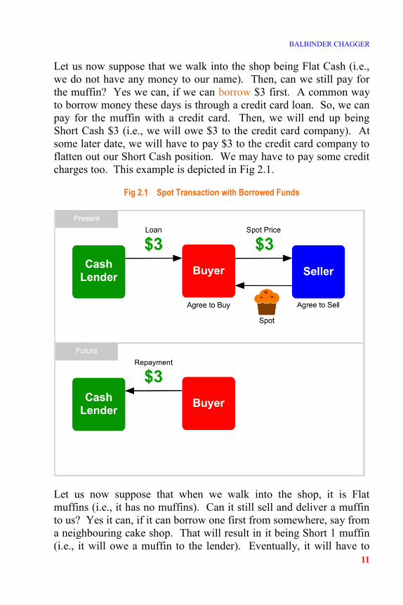
Let us now suppose that we walk into the shop being Flat Cash (i.e.,
we do not have any money to our name). Then, can we still pay for
the muffin? Yes we can, if we can borrow $3 first. A common way
to borrow money these days is through a credit card loan. So, we can
pay for the muffin with a credit card. Then, we will end up being
Short Cash $3 (i.e., we will owe $3 to the credit card company). At
some later date, we will have to pay $3 to the credit card company to
flatten out our Short Cash position. We may have to pay some credit
charges too. This example is depicted in Fig 2.1.
Fig 2.1 Spot Transaction with Borrowed Funds
Let us now suppose that when we walk into the shop, it is Flat
muffins (i.e., it has no muffins). Can it still sell and deliver a muffin
to us? Yes it can, if it can borrow one first from somewhere, say from
a neighbouring cake shop. That will result in it being Short 1 muffin
(i.e., it will owe a muffin to the lender). Eventually, it will have to

OPTIONS EXPLAINED SIMPLY: THE FUNDAMENTAL PRINCIPLES COURSE
12
return a muffin to the lender, and, perhaps, pay some borrowing
charges too. In reality though, it is unlikely that the shop would
borrow a muffin in this manner because muffins just are not lent and
borrowed in the world as readily as cash is. But other assets are, e.g.,
Stocks. There are lots of large pension companies out there that are
sitting on huge Long Stock positions. They are only too happy to
earn some extra income by lending their Stocks out in return for fees.
2.2 Short Position Types
Recall that we can sell and deliver an asset without owning it first.
The asset can be borrowed from a lender first, and then it can be
delivered to the buyer. Thus, we end up with a Short position in the
asset, which we will have to settle up later on.
There are two types of Short positions, as follows:
Covered Short
Uncovered Short
A Covered Short sale entails selling an asset Short in the certain
knowledge that we will receive a supply of the asset at a later date and
at a known cost. A Covered Short sale is depicted, in 4 steps, in Fig
2.2. The supply received is applied to settle up and close out the
Short position. A Covered Short sale is, therefore, a riskless strategy,
meaning the end profit is determinable from the outset (i.e., at the
time of the sale). The profit is based essentially on the following
facts, which are known with certainty at the time of the sale:
The Spot Price of the sale.
The cost of the anticipated supply.

BALBINDER CHAGGER
13
Fig 2.2 Covered Short Sale
To determine the complete profit, there will be other details to take
into account too, like the following:
The cost of borrowing the asset.
The interest income that can be earned on the sale proceeds.
These details too can be known with certainty at the time of the sale
and factored into the profit calculation.
To exemplify a Covered Short sale, let us say that an Apple company
employee is informed today officially that in a month from now she
will be awarded a bonus in the form of 100 Apple company shares.
Even though she will not legally own the shares until a month from
now, her financial interest in them begins today. Today, she knows

OPTIONS EXPLAINED SIMPLY: THE FUNDAMENTAL PRINCIPLES COURSE
14
what the Spot Price of the shares on the Stock market is. Let us say it
is $120 per share. It could go up or down over the next month. So,
she has no idea what the shares will be worth on the day she becomes
their legal owner. Her risk is that they might be worth less than they
are today. If she is happy with their $120 market value today, then
she can eliminate her risk by selling Short 100 shares today. The sale
will be a Covered Short sale because it is done in the certain
knowledge that the 100 shares will be received in a month’s time at
no cost.
The Short sale will give her a Long Cash position of $12,000
(100 × 120) and a Short Stock position of 100 Apple shares. She can
determine her end profit right from the outset (i.e., the time of the
sale) to be $12,000 (12,000 − 0), plus any interest she can earn on
the $12,000 sale proceeds and less any charges payable on borrowing
the shares for the Short sale.
In contrast, an Uncovered Short sale entails selling an asset without
an anticipated future supply of it at a known cost. At some time in the
future, the Short position will need to be closed out. That will have to
be done by buying the asset on the open market at the prevailing Spot
Price, which is an unknown figure when the Short sale is made. The
Uncovered Short sale is depicted, in 4 steps, in Fig 2.3.
An Uncovered Short sale is, therefore, a risky, speculative strategy,
meaning the end profit is undeterminable at the time of the sale
because the cost of the asset is unknown. The sale is based on the
speculative view that the Spot Price will drop so that the asset will be
bought back cheaper than it was sold for. But, there may be the
chance that the asset’s Spot Price increases. Then, it will have to be
purchased at a higher Spot Price than it was sold for, and will result in
a financial loss. The actual result cannot be known at the time of the
sale, and can go either way.

BALBINDER CHAGGER
15
Fig 2.3 Uncovered Short Sale

OPTIONS EXPLAINED SIMPLY: THE FUNDAMENTAL PRINCIPLES COURSE
16

BALBINDER CHAGGER
17
Lesson 3
SPOTS RISKS
In this lesson, we will learn about the risk that Spots give exposure to.
3.1 Risk Source
The financial value of a Stock position depends on the following
factors:
Number of shares (Quantity)
Type of position (Long or Short)
Market price of a share (Spot Price)
We can express this mathematically as follows:
𝑆𝑝𝑜𝑡𝑉𝑎𝑙𝑢𝑒 = 𝑄𝑢𝑎𝑛𝑡𝑖𝑡𝑦 × 𝑆𝑝𝑜𝑡𝑃𝑟𝑖𝑐𝑒
The number of shares we hold is under our complete control. We can
buy and sell them as we wish, and adjust our position to suit our
desire. But, we have no control whatsoever over the Spot Price; the
market determines it. We have to accept the Spot Price, whatever it
OPTIONS EXPLAINED SIMPLY: THE FUNDAMENTAL PRINCIPLES COURSE
18
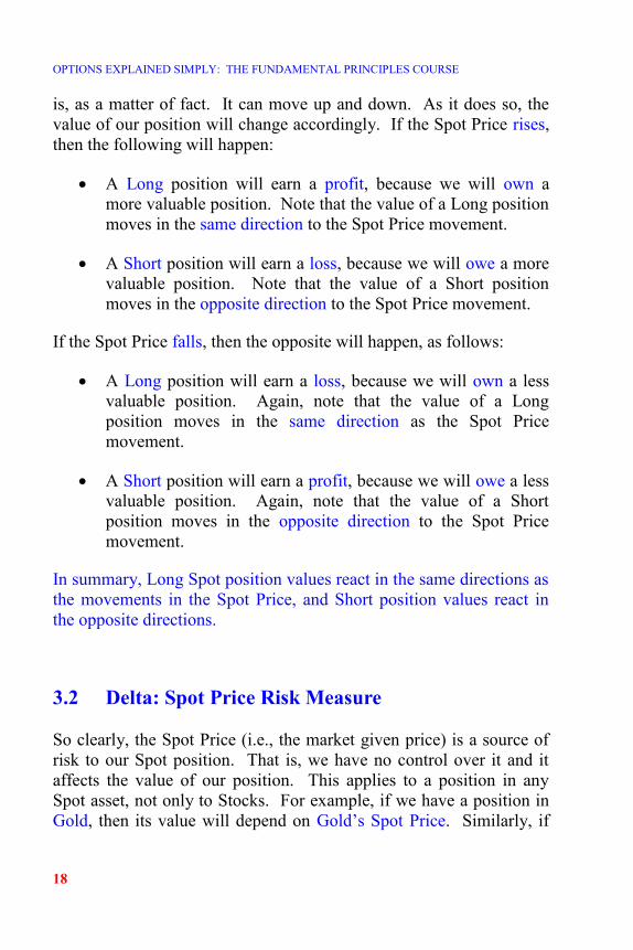
is, as a matter of fact. It can move up and down. As it does so, the
value of our position will change accordingly. If the Spot Price rises,
then the following will happen:
A Long position will earn a profit, because we will own a
more valuable position. Note that the value of a Long position
moves in the same direction to the Spot Price movement.
A Short position will earn a loss, because we will owe a more
valuable position. Note that the value of a Short position
moves in the opposite direction to the Spot Price movement.
If the Spot Price falls, then the opposite will happen, as follows:
A Long position will earn a loss, because we will own a less
valuable position. Again, note that the value of a Long
position moves in the same direction as the Spot Price
movement.
A Short position will earn a profit, because we will owe a less
valuable position. Again, note that the value of a Short
position moves in the opposite direction to the Spot Price
movement.
In summary, Long Spot position values react in the same directions as
the movements in the Spot Price, and Short position values react in
the opposite directions.
3.2 Delta: Spot Price Risk Measure
So clearly, the Spot Price (i.e., the market given price) is a source of
risk to our Spot position. That is, we have no control over it and it
affects the value of our position. This applies to a position in any
Spot asset, not only to Stocks. For example, if we have a position in
Gold, then its value will depend on Gold’s Spot Price. Similarly, if
BALBINDER CHAGGER
19
we have a position in Crude Oil, then its value will depend on Crude
Oil’s Spot Price.
It is very long-winded to have to say how a position’s value changes
relative to Spot Price movements. So, everyone in the Financial
Investment world just says Delta instead, for short. Delta is the
formal name given to the relationship between the Spot Price and the
position’s value. If someone says he has a Delta in Coffee, then
everyone understands that he has a position whose value reacts to
movements in the Spot Price of Coffee. In other words, the person
has a risk exposure to the Spot Price of Coffee.
It would be useful to know the following things also about the
position:
Whether its value reacts in the same or opposite direction to
the Spot Price movement.
The size of the reaction.
The Financial Investment world has thought about these aspects and
agreed standard ways to communicate them, as follows:
The term Long is used to communicate that the position value
changes in the same direction as the Spot Price movement.
The term Short is used to communicate that the position value
changes in the opposite direction to the Spot Price movement.
A number is used to communicate the amount the position
value changes.
The number communicates the amount by which the position
value changes as the Spot Price increases by 1.
The number is calculated under the assumption that all other
factors that affect the position’s value remain static while only
the Spot Price increases. Later, when we look at Forwards and

OPTIONS EXPLAINED SIMPLY: THE FUNDAMENTAL PRINCIPLES COURSE
20
Options, we will appreciate that there are other factors besides
Spot Price that affect some positions’ values.
Delta is a standardised Risk Measure; it communicates, in a
standardised way, how a position’s value reacts to the Spot Price. It is
the first of several risk measures that we will encounter as we
progress through this course.
If someone says he is Long 100 Delta in Corn, then everyone
understands that he has a risk exposure to Corn’s Spot Price such that
if it rises by $1, then he will make a $100 profit. Similarly, if
someone says he is Short 200 Delta in Crude Oil, then everyone
understands that he has a risk exposure to Crude Oil’s Spot Price such
that if it rises by $1, then he will suffer a $200 loss.
Delta can be expressed mathematically as follows:
𝐷𝑒𝑙𝑡𝑎 =𝐶ℎ𝑎𝑛𝑔𝑒𝐼𝑛𝑃𝑜𝑠𝑖𝑡𝑖𝑜𝑛𝑉𝑎𝑙𝑢𝑒
𝑅𝑖𝑠𝑒𝐼𝑛𝑆𝑝𝑜𝑡𝑃𝑟𝑖𝑐𝑒
The Delta value communicates a Rate of Change (the rate at which
the Position Value changes as the Spot Price increases by 1).
A Rate of Change tells us how much something changes for a given
change in something else. It can be thought of as a gradient, telling us
the degree of change. A flat, horizontal gradient tells us that there is
no change. An upward gradient tells us that the change is in the same
direction, while a downward gradient tells us that the change is in the
opposite direction. The steeper the gradient, the larger is the reaction
to a rise in the factor. Furthermore, a Rate of Change value
corresponds to a specific point. At another point, the Rate of Change
may be a different value. These aspects are illustrated in Fig 3.1.
Inflation is an example of a Rate of Change that we are all familiar
with. It is useful to use it to understand the above aspects of Rates of
Changes. Inflation tells us how the cost of things reacts to the passing
of time (usually 1 year). An Inflation value of, say, 3% tells us that
things costing $100 today will cost $103 in a year from now. The 3%
value corresponds to now. Next month (i.e., at a different point in

BALBINDER CHAGGER
21
time), Inflation could be some other value, say 2.9%. Likewise, a
Delta value corresponds to a specific Spot Price. At another Spot
Price, it can be another value.
Fig 3.1 Rates of Change
3.3 Delta of a Long Stock Position
The value of a Long Stock position is calculated as follows:
𝑆𝑝𝑜𝑡𝑉𝑎𝑙𝑢𝑒 = 𝑁𝑢𝑚𝑏𝑒𝑟𝑂𝑓𝑆ℎ𝑎𝑟𝑒𝑠 × 𝑆𝑝𝑜𝑡𝑃𝑟𝑖𝑐𝑒
The value of a Long 1-share position at various Spot Prices is shown
in Fig 3.2.

OPTIONS EXPLAINED SIMPLY: THE FUNDAMENTAL PRINCIPLES COURSE
22
Fig 3.2 Long Stock vs Spot Price
Each of the Spot Price increments is $100. When the Spot Price is $0,
then the position value is also $0. As the Spot Price rises, the value of
the position also rises. That signifies that the Delta is positive (Long).
We can see in Fig 3.2 that the position value rises by a constant $100
for every $100 rise in the Spot Price (i.e., $1 for $1 reaction). That
signifies that the Delta is +1 (or +100%) at every Spot Price (100 ÷100). That is corroborated by the fact that a graph plot of the position
value against the Spot Price (Fig 3.3) shows all the position values
sitting on an upward sloping straight line whose gradient is +1.
We can prove mathematically that the Delta value is +1 at a particular
Spot Price. A simple way to calculate the Delta at a particular
observation point is to look at how the position value changes
between two points either side of it, such that the observation point
lies exactly in the middle of them. For example, to calculate the Delta
at the $500 Spot Price, consider how the position’s value changes
from a Spot Price of $400 to $600. This simple calculation is possible
because the $500 Spot Price lies exactly in the middle of the $400 to
$600 Spot Price range.
𝐷𝑒𝑙𝑡𝑎 =𝐶ℎ𝑎𝑛𝑔𝑒𝐼𝑛𝑃𝑜𝑠𝑖𝑡𝑖𝑜𝑛𝑉𝑎𝑙𝑢𝑒
𝑅𝑖𝑠𝑒𝐼𝑛𝑆𝑝𝑜𝑡𝑃𝑟𝑖𝑐𝑒
𝐷𝑒𝑙𝑡𝑎 =𝐹𝑖𝑛𝑎𝑙𝑉𝑎𝑙𝑢𝑒 − 𝐼𝑛𝑖𝑡𝑖𝑎𝑙𝑉𝑎𝑙𝑢𝑒
𝐹𝑖𝑛𝑎𝑙𝑆𝑝𝑜𝑡𝑃𝑟𝑖𝑐𝑒 − 𝐼𝑛𝑖𝑡𝑖𝑎𝑙𝑆𝑝𝑜𝑡𝑃𝑟𝑖𝑐𝑒

BALBINDER CHAGGER
23
𝐷𝑒𝑙𝑡𝑎 =600 − 400
600 − 400=
200
200= +1.0
The Delta at all the other Spot Prices in Fig 3.2 can be calculated in
this way.
Fig 3.3 Long Stock vs Spot Price
When the relationship between two things (in this case, the
relationship between a Spot Price and a Position Value) remains the
same over a range of values, then the relationship is said to be linear
over that range. So, the Delta of a Long 1-share position is linear and
is +1 (or +100%). This applies to all Spot types, not to Stocks only.
So, we can generalise and say that the Delta of a Long 1 unit of a Spot
is linear and +1 (or +100%).
OPTIONS EXPLAINED SIMPLY: THE FUNDAMENTAL PRINCIPLES COURSE
24
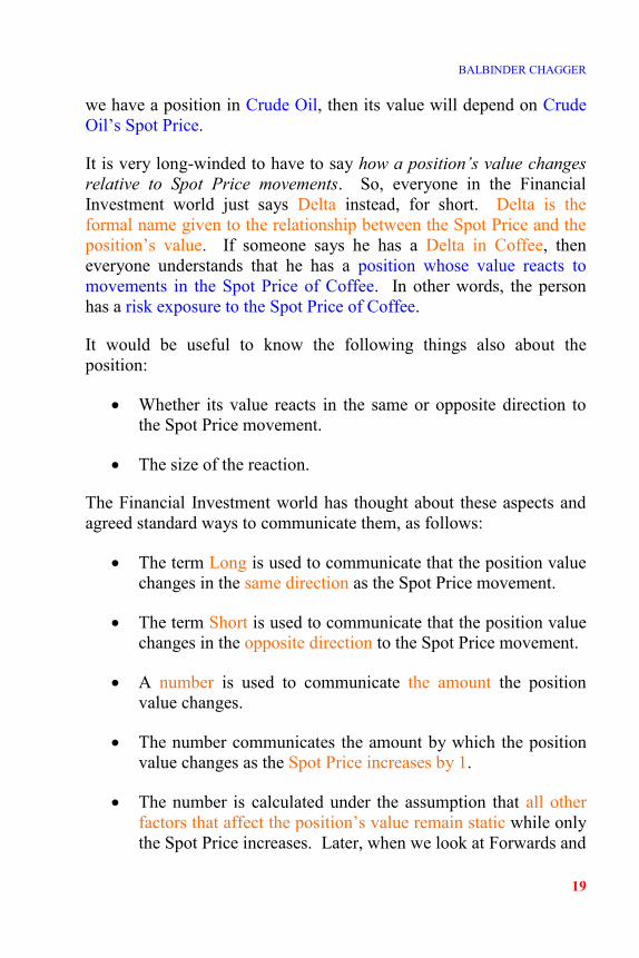
Fig 3.4 shows the Delta of the Spot plotted against the Spot Price.
The Delta is +1 at every Spot Price.
Fig 3.4 Long Stock Delta vs Spot Price
As the Delta of a Long 1-share position is +1 (or +100%), then it
follows that the Delta of a Long 2-share position will be +2 (or
+200%), and so on for larger numbers of shares. So, if someone says
their holding in a Stock gives them a 300 Delta exposure, then we can
say the following:
The person is Long 300 shares (because the Delta of a Long
1-share position is +1).
If the Spot Price rises by $1, then the person will earn a profit
of $300.
As we know this is a Stock position and that the Delta of Stock is
linear, then we can also say how the position value will react to any
amount of change in the Spot Price, not only to a rise of $1. For
example, we can say the following:
If the Spot Price falls by $1, then the person will suffer a loss
of $300.
If the Spot Price rises by $20.5, then the person will profit
$6,150 (20.5 × 300).

BALBINDER CHAGGER
25
When a position’s Delta is linear, then the change in the position’s
value due to a Spot Price movement is explained completely as
follows:
𝐶ℎ𝑎𝑛𝑔𝑒𝐼𝑛𝑉𝑎𝑙𝑢𝑒 = 𝐷𝑒𝑙𝑡𝑎 × 𝐶ℎ𝑎𝑛𝑔𝑒𝐼𝑛𝑆𝑝𝑜𝑡𝑃𝑟𝑖𝑐𝑒
𝐶ℎ𝑎𝑛𝑔𝑒𝐼𝑛𝑉𝑎𝑙𝑢𝑒 = 𝐷𝑒𝑙𝑡𝑎 × (𝐹𝑖𝑛𝑎𝑙𝑆𝑝𝑜𝑡𝑃𝑟𝑖𝑐𝑒 − 𝐼𝑛𝑖𝑡𝑖𝑎𝑙𝑆𝑝𝑜𝑡𝑃𝑟𝑖𝑐𝑒)
Later, when we study Futures and Options, we will see that Delta can
take on other values besides 1 (or 100%). Furthermore, we will see
that Delta can also be non-linear, meaning that it can be a different
value at different Spot Prices.
3.4 Delta of a Short Stock Position
As the Delta of a Long 1-share position is linear and +1, then it
follows that the Delta of a Short 1-share position will be linear and -1
(or -100%).
The value of a Short Stock position is calculated as follows:
𝑆𝑝𝑜𝑡𝑉𝑎𝑙𝑢𝑒 = −𝑁𝑢𝑚𝑏𝑒𝑟𝑂𝑓𝑆ℎ𝑎𝑟𝑒𝑠 × 𝑆𝑝𝑜𝑡𝑃𝑟𝑖𝑐𝑒
The – sign denotes the position is Short. The value of a Short 1-share
position at various Spot Prices is shown in Fig 3.5.
Fig 3.5 Short Stock vs Spot Price

OPTIONS EXPLAINED SIMPLY: THE FUNDAMENTAL PRINCIPLES COURSE
26
Each of the Spot Price increments is $100. As the Spot Price rises,
the value of the position falls (i.e., it becomes a larger negative
number), as we would expect. Therefore, the Delta is negative
(Short). The position value falls by a constant $100 for every $100
rise in the Spot Price (i.e., -$1 for +$1). Therefore, the Delta is -1 (or
-100%) at every Spot Price. That is corroborated by the fact that a
graph plot of the position value against the Spot Price (Fig 3.6) shows
all the position values sitting on a downward sloping straight line
whose gradient is -1. So, the Delta of a Short 1-share position is
linear and is -1 (or -100%). Again, this applies to all Spot positions,
not to Stocks only. So again, we can generalise and say that the Delta
of a Short 1 unit of a Spot position is linear and -1 (or -100%).
Fig 3.6 Short Stock vs Spot Price
BALBINDER CHAGGER
27
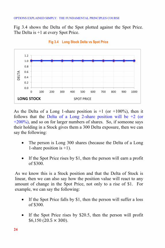
Fig 3.7 shows the Delta of the Spot plotted against the Spot Price.
The Delta is -1 at every Spot Price.
Fig 3.7 Short Stock Delta vs Spot Price
If someone says their holding in a Stock gives them a -500 Delta
exposure, then we can say the following:
The person is Short 500 shares (because the Delta of 1 Short
Stock is -1).
If the Spot Price rises by $1, then the person will suffer a
$500 loss.
As we know this is a Stock position and the Delta of Stock is linear,
then we can also say how the position value will react to any amount
of change in Spot Price, not only to a rise of $1. For example:
If the Spot Price falls by $1, then the person will profit $500.
If the Spot Price drops by $32.25, then the person will profit
$16,125 (−32.25 × −500).

OPTIONS EXPLAINED SIMPLY: THE FUNDAMENTAL PRINCIPLES COURSE
28
BALBINDER CHAGGER
29
Lesson 4
ARBITRAGE
In this lesson, we will learn what Arbitrage is and why it is important.
Arbitrage is the concept of profiting by exploiting price imbalances.
There are two types of arbitrage, as follows:
1. Deterministic Arbitrage
2. Statistical Arbitrage
4.1 Deterministic Arbitrage
The nature of an arbitrage opportunity is Deterministic if the profit
from it can be determined from the outset with absolute certainty, i.e.,
there is no risk involved.
For example, let us suppose a company’s shares are trading for £10 on
the London Stock Exchange and for $13 on the New York Stock
Exchange while the £/$ currency exchange rate is £1=$1.2. As the
shares are of the one and the same company, then their value ought to

OPTIONS EXPLAINED SIMPLY: THE FUNDAMENTAL PRINCIPLES COURSE
30
be equal, regardless of the location. But, as it stands, they are not
equal. The London £10 Spot Price implies that the New York Spot
Price ought to be $12. Likewise, the New York $13 Spot Price
implies that the London Spot Price ought to be £10.83. Instead of
being equal, the Spot Prices have spread apart by $1 (£0.83), for some
reason, and are imbalanced, as depicted in Fig 4.1. The Spot Price in
London is cheaper than the one in New York. This price imbalance
may be due to some kind of market inefficiency; perhaps some news
has reached one location but not yet the other. The reason is
unimportant. The fact is that the Spot Prices are out of line with each
other, and the situation presents an opportunity to make a certain
profit of $1 (£0.83).
Fig 4.1 Deterministic Arbitrage Opportunity
We can exploit this arbitrage opportunity by executing two Spot
trades simultaneously; one, buying the relatively cheaper London
share, and the other, selling the relatively expensive New York share.
The London trade makes us Long 1 share, for which we pay out £10
($12), and the New York trade makes us Short 1 share, for which we
receive $13 (£10.83). The cashflows sum to a profit of $1 (£0.83).
Note that the Long position gives us a +1 Delta risk exposure, and the
Short position, a -1 Delta. Although we actually have 2 separate
positions across 2 locations, overall we have no Delta risk exposure

BALBINDER CHAGGER
31
(+1 and -1 sum to 0). This means that our portfolio (i.e., the
combined positions) will neither benefit nor suffer in value from any
Spot Price movements; gains on one position will be offset by losses
on the other, and vice versa.
Our act of buying the London share contributes (albeit in a miniscule
way) to raising the demand for it in the market. That, in turn, tends to
raise its Spot Price. Similarly, our act of selling the New York share
contributes to lowering its demand and, hence, its Spot Price too. In
other words, our trades contribute to influencing the Spot Prices back
into a balanced state by tending to narrow the Price Spread that exists
between them. Other Arbitrage traders who also spot this opportunity
will exploit it in the same way as we did. The collective influence of
everyone’s trades will tend to drive the Spot Prices into balance so
that the Price Spread between them tends to narrow and disappear,
until there is no longer any arbitrage opportunity remaining to be
exploited. That is the importance of Deterministic Arbitrage; it drives
imbalanced prices back into alignment, as depicted in Fig 4.2.
Fig 4.2 Deterministic Arbitrage’s Role
There are lots of possible combinations of Spot Price and £/$
Exchange Rate at which these two share prices can be in alignment
with each other. Let us say that alignment occurs at Spot Prices £9.70
and $11.155, and at an exchange rate of £1=$1.15. Then, we have

OPTIONS EXPLAINED SIMPLY: THE FUNDAMENTAL PRINCIPLES COURSE
32
exploited the arbitrage opportunity fully and we should trade out of
our positions and exit the strategy. On selling down our Long
position in London, we receive £9.70 ($11.155), and on buying up our
Short position in New York, we pay out $11.155 (£9.70). The
cashflows sum to $0 (£0). We make neither a profit nor a loss on
trading out of the strategy. We retain the sum cashflow of $1 ($0.83)
that we collected on entering the strategy. Thus, we profit $1 (£0.83),
as we had determined from the outset.
4.2 Statistical Arbitrage
The nature of an arbitrage opportunity is Statistical if the profit from
it cannot be determined from the outset with absolute certainty, i.e.,
risk is involved. This means that we expect theoretically to make a
particular amount of profit, but in practice we are not certain to realise
our expectation because there is risk inherent in the situation.
For example, let us say there is a game where a fair 6-sided die is
rolled and the player receives the dollar value of the number that is
rolled. So, if a 4 is rolled, then the player receives $4. Let us also say
that the game costs $3 to play per go. Then, the possible outcomes
are shown in Fig 4.3.
Fig 4.3 Die Game

BALBINDER CHAGGER
33
We cannot say for certain how much we will win in this game
because we cannot say which number will turn up; there is risk
involved. We know there are 6 numbers on a die and that the die is
fair. So, the chance of any number being rolled is equal, and is 1/6.
If we play this game once only, then the 1/6 chance value is
meaningless and irrelevant. We could be very unlucky and end up $2
out of pocket because we rolled a 2, or we could be very lucky and
end up $3 better off because we rolled a 6.
But, if we play this game repeatedly, then the 1/6 chance value
becomes meaningful and relevant. We expect rolled numbers to
average out to 3.5, meaning we expect to make an arbitrage profit of
$0.50 per play (3.5 − 3). This is depicted in Fig 4.4. Note that our
expectation of $0.50 profit can never be realised on any single play
though, because a die does not have a face with 31/2 dots on it. So,
3.5 can never actually be rolled, and we can never actually make a
$0.50 profit on any single throw. Understand then that an Expected
Value is a theoretical value; it may or may not be one of the possible
real outcomes.
Fig 4.4 Statistical Arbitrage Opportunity
So, what we have in this game is a theoretical arbitrage profit
opportunity of $0.50 per play. After 100 plays, we expect to make
$50 (100 × 0.50). However, our expectation is not guaranteed to
materialise. The $50 profit is a theoretical result based on the 1/6
probability of each number being rolled. The number of times each

OPTIONS EXPLAINED SIMPLY: THE FUNDAMENTAL PRINCIPLES COURSE
34
number actually gets rolled may be somewhat different to what the
probabilities suggested. But the more times we play, the more the
probabilities will get borne out and the closer will our profit be to our
expectation. That is the nature of probabilities; they are based on the
notion of infinite trials. After 1,000 plays, we expect to make $500
(1000 × 0.50). After 10,000 plays, we expect to make $5,000
(10000 × 0.50). So, we should keep playing this game over and over
again, infinite times, because then we would make an infinite profit.
As we play this game more and more times, the game organiser will
suffer an increasing amount of loss. This ought to trigger him to
review the price per play and increase it to $3.50, where the statistical
arbitrage opportunity disappears. At $3.50 per play, there will be no
arbitrage opportunity and so, players will be indifferent to playing.
That is the importance of Statistical Arbitrage; it drives imbalanced
prices back into alignment, as depicted in Fig 4.5, just as
Deterministic Arbitrage does too.
Fig 4.5 Statistical Arbitrage’s Role
At a price per play above $3.50, the game organiser will be the one
who expects to make the profit. You might be thinking that nobody
would play such a game, but you would be wrong; the Gambling
industry is built on this type Statistical Arbitrage opportunity.
In order to take advantage of Statistical Arbitrage opportunities, the
following conditions are necessary:
BALBINDER CHAGGER
35
Correct outcomes and probability values - so that correct
Expected Values can be determined. In the die game example
above, it is possible to determine the outcomes and their
probabilities absolutely because everything in the game is
known and understood fully. However, in investment
scenarios, some outcomes and their probabilities might have to
be estimated or guessed.
A large number of goes/plays - so that the probabilities
become borne out.
Sufficient funds - to be able to keep playing. A series of loss
making outcomes might occur before any profiting ones. If
the losses incurred wipe out the funds needed to keep playing,
then the large number of outcomes necessary for the
probabilities to be borne out cannot occur and the expected
profit can never be realised.

OPTIONS EXPLAINED SIMPLY: THE FUNDAMENTAL PRINCIPLES COURSE
36

BALBINDER CHAGGER
37
Lesson 5
RATIONALITY
In this lesson, we will learn that the study of financial concepts calls
for objective, rational thinking.
In the Deterministic Arbitrage example in Lesson 4, the London Stock
was cheaper than the New York Stock. We bought the cheaper Stock
and sold the more expensive one, simultaneously. Suppose instead
we had bought the London Stock only, because it was the cheaper
one. Then, we would have a +1 Delta risk exposure, meaning
movements in the Spot Price (over which we have no control) would
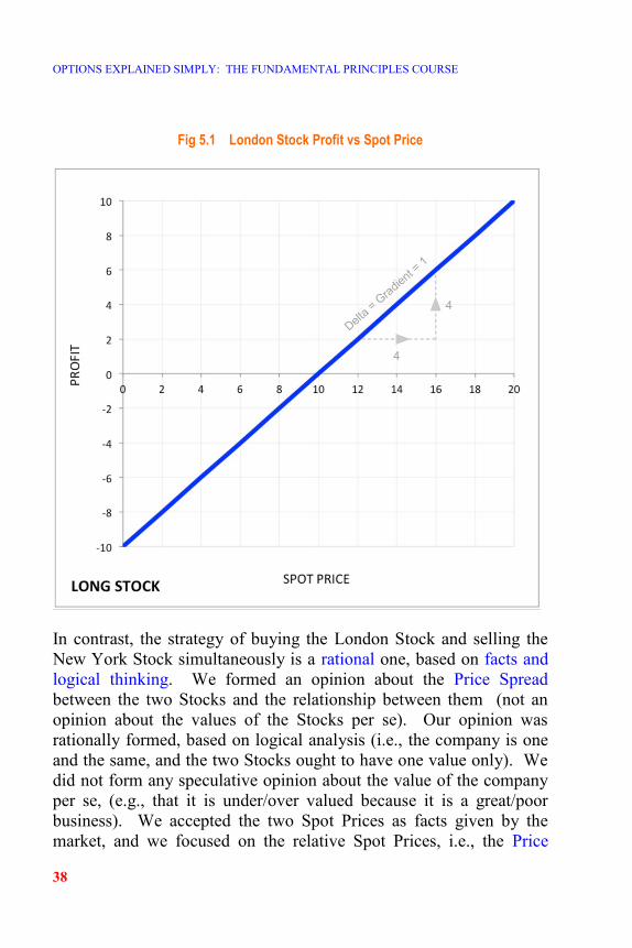
cause us gains or losses, as shown in Fig 5.1.
If the Spot Price rises above £10, then we will profit. But, it can fall.
Then, we will suffer loss. We know neither in which direction nor by
how much the Spot Price will move. So, buying the London Stock
only is a risky investment strategy. It is a speculative strategy based
on a subjective opinion that the Spot Price will rise. We cannot be
certain that it will rise. Suppose the company goes bust, which is a
possibility. Then, the Spot Price will crash to £0 and we will lose the
whole of our £10 investment. This strategy is based on speculation,
entailing subjective opinions, hope and prayer.
OPTIONS EXPLAINED SIMPLY: THE FUNDAMENTAL PRINCIPLES COURSE
38
Fig 5.1 London Stock Profit vs Spot Price
In contrast, the strategy of buying the London Stock and selling the
New York Stock simultaneously is a rational one, based on facts and
logical thinking. We formed an opinion about the Price Spread
between the two Stocks and the relationship between them (not an
opinion about the values of the Stocks per se). Our opinion was
rationally formed, based on logical analysis (i.e., the company is one
and the same, and the two Stocks ought to have one value only). We
did not form any speculative opinion about the value of the company
per se, (e.g., that it is under/over valued because it is a great/poor
business). We accepted the two Spot Prices as facts given by the
market, and we focused on the relative Spot Prices, i.e., the Price

BALBINDER CHAGGER
39
Spread, the source of our profit. The trades we executed homed in on
and exposed us to the Price Spread only, not to any Spot Price.
Fig 5.2 London and New York Stock Profit vs Spot Price
We did not care where the Spot Prices moved to except for them to
come into alignment at some point. Even if the company went bust
and the Spot Prices became £0 and $0, our strategy would still have
worked as we had determined, as can be seen in Fig 5.2, because the
prices would be in alignment then too.
So, understand that the study of Derivatives calls for the application
of objective, rational thinking.


