

IEEE TRANSACTIONS ON VISUALIZATION & COMPUTER GRAPHICS 1
Data-Parallel Octrees for Surface Reconstruction
Kun Zhou∗ Minmin Gong† Xin Huang† Baining Guo†
∗State Key Lab of CAD&CG, Zhejiang University †Microsoft Research Asia
Abstract—We present the first parallel surface reconstructionalgorithm that runs entirely on the GPU. Like existing implicitsurface reconstruction methods, our algorithm first builds anoctree for the given set of oriented points, then computesan implicit function over the space of the octree, and finallyextracts an isosurface as a water-tight triangle mesh. A keycomponent of our algorithm is a novel technique for octreeconstruction on the GPU. This technique builds octrees inreal-time and uses level-order traversals to exploit the fine-grained parallelism of the GPU. Moreover, the techniqueproduces octrees that provide fast access to the neighborhoodinformation of each octree node, which is critical for fastGPU surface reconstruction. With an octree so constructed,our GPU algorithm performs Poisson surface reconstruction,which produces high quality surfaces through a global opti-mization. Given a set of 500K points, our algorithm runs atthe rate of about five frames per second, which is over twoorders of magnitude faster than previous CPU algorithms. Todemonstrate the potential of our algorithm, we propose a user-guided surface reconstruction technique which reduces thetopological ambiguity and improves reconstruction results forimperfect scan data. We also show how to use our algorithmto perform on-the-fly conversion from dynamic point clouds tosurfaces as well as to reconstruct fluid surfaces for real-timefluid simulation.
Index Terms—surface reconstruction, octree, programablegraphics unit, marching cubes
I. Introduction
Surface reconstruction from point clouds has been an active
research area in computer graphics. This reconstruction
approach is widely used for fitting 3D scanned data, filling
holes on surfaces, and remeshing existing surfaces. So
far, surface reconstruction has been regarded as an off-
line process. Although there exist a number of algorithms
capable of producing high-quality surfaces, none of these
can achieve interactive performance.
In this paper we present a parallel surface reconstruction
algorithm that runs entirely on the GPU. Following previous
implicit surface reconstruction methods, our algorithm first
builds an octree for the given set of oriented points,
then computes an implicit function over the space of the
octree, and finally extracts an isosurface as a water-tight
triangle mesh using the marching cubes. Unlike previous
methods which all run on CPUs, our algorithm performs
all computation on the GPU and capitalizes on modern
GPUs’ massively parallel architecture. Given a set of 500K
points, our algorithm runs at the rate of about five frames
per second. This is over two orders of magnitude faster than
previous CPU algorithms.
Fig. 1: Our GPU reconstruction algorithm can generate
high quality surfaces with fine details from noisy real-world
scans. The algorithm runs at interactive frame rates. Top
left: Bunny, 350K points, 5.2 fps. Top right: Dragon, 1500K
points, 1.3 fps. Bottom left: Buddha, 640K points, 4 fps.
Bottom right: Armadillo, 500K points, 5 fps.
The basis of our algorithm is a novel technique for fast
octree construction on the GPU. This technique has two
important features. First, it builds octrees in real-time by
exploiting the fine-grained parallelism on the GPU. Unlike
conventional CPU octree builders, which often construct
trees by depth-first traversals, our technique is based on
level-order traversals: all octree nodes at the same tree level
are processed in parallel, one level at a time. Modern GPU
architecture contains multiple physical multi-processors and
requires tens of thousands of threads to make the best use
of these processors [1]. With level-order traversals, our
technique maximizes the parallelism by spawning a new
thread for every node at the same tree level.
The second feature of our technique is that it constructs
octrees that supply the information necessary for GPU
surface reconstruction. In particular, it is critical for the
octree data structure to provide fast access to tree nodes as
well as the neighborhood information of each node (i.e.
links to all neighbors of the node), which are required
by the implicit function computation and marching cubes
IEEE TRANSACTIONS ON VISUALIZATION & COMPUTER GRAPHICS 2
algorithms described in Section IV. While information of
individual nodes is relatively easy to collect, computing
the neighborhood information requires a large number of
searches for every single node. Collecting neighborhood
information for all nodes of the tree is thus extremely
expensive even on the GPU. To address this problem, we
make the observation that a node’s neighbors are deter-
mined by the relative position of the node with respect to its
parent and its parent’s neighbors. Based on this observation,
we build two look up tables (LUT) which record the relative
pointers to a node’s relatives. Unlike direct pointers, relative
pointers are independent of specific instances of octrees and
hence can be precomputed. At runtime, the actual pointers
are quickly generated by querying the LUTs.
Based on octrees built as above, we develop a GPU al-
gorithm for the Poisson surface reconstruction method [2].
We choose the Poisson method because it can reconstruct
high quality surfaces through a global optimization. As part
of our GPU algorithm, we derive an efficient procedure for
evaluating the divergence vector in the Poisson equation
and an adaptive marching cubes procedure for extracting
isosurfaces from an implicit function defined over the
volume spanned by an octree. Both of these procedures
are designed to fully exploit modern GPUs’ fine-grained
parallel architecture and make heavy use of the octree
neighborhood information. Note that GPU algorithms can
also be readily designed for classical implicit reconstruc-
tion methods (e.g. [3]) by using our octree construction
technique and the adaptive marching cubes procedure, as
described in the last paragraph of Section IV-D. Therefore,
our work provides a general approach for designing GPU
algorithms for surface reconstruction.
Our GPU surface reconstruction can be employed im-
mediately in existing applications. As an example, we
propose a user-guided reconstruction algorithm for im-
perfect scan data where many areas of the surface are
either under-sampled or completely missing. Similar to a
recent technique [4], our algorithm allows the user to draw
strokes around poorly-sampled areas to reduce topological
ambiguities. Benefiting from the high performance of GPU
reconstruction, the user can view the reconstructed mesh
immediately after drawing a stroke. In contrast, the algo-
rithm described in [4] requires several minutes to update
the reconstructed mesh, although it is able to update the
implicit function within less than a second.
GPU surface reconstruction also opens up new possibilities.
As an example, we propose an algorithm for generating
surfaces for dynamic point clouds on the fly. The recon-
structed meshes may be directly rendered by the tradi-
tional polygon-based display pipeline. We demonstrate the
application of our algorithm in two well-known modeling
operations, free-form deformation and boolean operations.
With advancements in commodity graphics hardware, real-
time surface reconstruction will be realized in the near
future. In view of this, our technique may be regarded as
a bridging connection between point- and polygon-based
representations. We also show our algorithm can be used to
reconstruct fluid surfaces for real-time particle-based fluid
simulation.
II. Related Work
Surface reconstruction from point clouds has a long history.
Here we only cover references most relevant to our work.
Early reconstruction techniques are based on Delaunay
triangulations or Voronoi diagrams ([5], [6]) and they build
surfaces by connecting the given points. These techniques
assume the data is noise-free and densely sampled. For
noisy data, postprocessing is often required to generate a
smooth surface ([7], [8]). Most other algorithms reconstruct
an approximating surface represented in implicit forms,
including signed distance functions ([3], [9], [10]), radial
basis functions ([11], [12], [13]), moving least square sur-
faces ([14], [15], [16]), and indicator functions [2]. These
algorithms mainly focus on generating high quality meshes
to optimally approximate or interpolate the data points.
Existing fast surface reconstruction methods are limited to
simple smooth surfaces or height fields. Randrianarivony
and Brunnett [17] proposed a parallel algorithm to ap-
proximate a point set with NURBS surfaces. Borghese
et al. [18] presented a real-time reconstruction algorithm
for height fields. For CAD applications, Weinert et al.
[19] used a parallel multi-population algorithm to find
a CSG representation that best fits data points. None of
these techniques is appropriate for reconstructing complex
surfaces from point clouds.
Recently, Buchart et al. [20] proposed a GPU interpolating
reconstruction method by using local Delaunay triangula-
tion [21]. First, the k-nearest neighbors to each point are
computed on the CPU. Then, for each point on the GPU, its
neighbors are ordered by angles around the point and the
local Delaunay triangulation is computed. For a moderate-
sized data set (e.g. 250K points), their algorithm needs over
10 seconds, which is still far from interactive performance.
In another recent work [22], both the k-nearest neighbors
and local Delaunay triangulation are computed on the
GPU. However, they need to build an octree on the CPU.
Moreover, these Delaunay triangulation based algorithms
can only handle noise-free and uniformly-sampled point
clouds. For noisy data, they may fail to produce a water-
tight surface.
With real-world scan data, some areas of the surface
may be under-sampled or completely missing. Automatic
techniques will fail to faithfully reconstruct the topology
of the surface around these areas. Recently Sharf et al.
[4] introduced a user-assisted reconstruction algorithm to
solve this problem. It asks the user to add local insid-
e/outside constraints at weak regions of unstable topology.
An optimal distance field is then computed by minimizing
a quadric function combining the data points, user con-
straints, and a regularization term. This system allows the
IEEE TRANSACTIONS ON VISUALIZATION & COMPUTER GRAPHICS 3
user to interactively draw scribbles to affect the distance
field at a coarse resolution, but the final surface reconstruc-
tion at finer resolutions takes several minutes, prohibiting
immediate viewing of the reconstructed mesh.
Octree is an important data structure in surface reconstruc-
tion algorithms. It is used for representing the implicit func-
tion ([13], [2]) and for adaptively extracting iso-surfaces
([23], [24]). Creating an octree for point clouds directly
on the GPU, however, is very difficult, mainly because of
memory allocation and pointer creation. Lefohn et al. [25]
described an abstraction and generic template library for
defining complex, random-access graphics processor (GPU)
data structures such as octrees. However, Lefohn et al. did
not describe a method for constructing octrees on the GPU.
Their octrees are constructed on the CPU and then sent to
the GPU. Recently, DeCoro and Tatarchuk [26] proposed
a real-time mesh simplification algorithm based vertex
clustering on the GPU. A probabilistic octree is built on the
GPU to support adaptive clustering. This octree, however,
does not form a complete partitioning of the volume and
only contains node information. Last year, Sun et al. [27]
proposed a method to construct an octree for a volume to
accelerate photon tracing. Their octree is represented as a
dense 3D array of numbers, where the value in each voxel
indicates the hierarchy level of the leaf node covering that
voxel. In other words, only leaf nodes are generated. Our
octrees are significantly more complicated than all these
octrees. Specifically, our octrees provide information about
vertices, edges and faces of octree nodes, as well as the
links to all neighbors of each octree node. This information
is necessary for GPU surface reconstruction.
There has been some concurrent work building spatial hier-
archies on the GPU, e.g. kd-trees [28] and BVHs (bounding
volume hierarchies) [29]. Similar to our algorithm, these
methods adopt breadth-first search construction order to
maximize GPU’s parallelism. The linear BVH construction
algorithm in [29] also uses the Morton codes (i.e. the
shuffled xyz keys) to build the hierarchy. However, none
of them can generate the information about vertices, edges
and faces of tree nodes, as well as the neighbors of each
tree node.
III. GPU Octree Construction
In this section, we describe how to build an octree Owith maximum depth D from a given set of sample points
Q = {qi | i = 1, ...N}. We first explain the design of
the octree data structure. Next we present a procedure for
the parallel construction of an octree with only individual
nodes. Then we introduce an LUT-based technique for ef-
ficiently computing the neighborhood information of every
octree node in parallel. Finally, we discuss how to collect
information of vertices, edges, and faces of octree nodes.
A. Octree Data Structure
The octree data structure consists of four arrays: vertex
array, edge array, face array, and node array. The vertex,
edge, and face arrays record the vertices, edges, and faces
of the octree nodes respectively. These arrays are relatively
simple. In the vertex array, each vertex v records v.nodes,
the pointers to all octree nodes that share vertex v. Follow-
ing v.nodes we can easily reach related elements such as
all edges sharing v. In the edge array, each edge records
the pointers to its two vertices. Similarly in the face array
each face records the pointers to its four edges.
The node array, which records the octree nodes, is more
complex. Each node t in the node array NodeArray needs
236 bytes and contains three pieces of information:
• The shuffled xyz key [23], t.key.
• The sample points contained in t.
• Pointers to related data including its parent, children,
neighbors, and other information as explained below.
Shuffled xyz Key: Since each octree node has eight
children, it is convenient to number a child node using
a 3-bit code ranging from zero to seven. This 3-bit code
encodes the subregion covered by each child. We use the
xyz convention: if the x bit is 1, the child covers an octant
that is “right in x”; otherwise the child covers an octant
that is “left in x”. The y and z bits are similarly set. The
shuffled xyz key of a node at tree depth D is defined as
the bit string
x1y1z1x2y2z2 · · · xDyDzD,
indicating the path from the root to this node in the octree.
Therefore a shuffled xyz key at depth D has 3D bits.
Currently we use 32 bits to represent the key, allowing a
maximum tree depth of 10. The unused bits are set to zero.
Sample Points: Each octree node records the sample points
enclosed by the node. The sample points are stored in a
point array and sorted such that all points in the same node
are contiguous. Therefore, for each node t, we only need
to store the number of points enclosed, t.pnum, and the
index of the first point, t.pidx, in the point array.
Connectivity Pointers: For each node we record the point-
ers to the parent node, 8 child nodes, 27 neighboring nodes
including itself, 8 vertices, 12 edges, and 6 faces. All point-
ers are represented as indices to the corresponding arrays.
For example, t’s parent node is NodeArray[t.parent] and
t’s first neighboring node is NodeArray[t.neighs[0]]. If
the pointed element does not exist, we set the corresponding
pointer to −1. Since each node has 27 neighbors at the same
depth, the array t.neighs is of size 27.
For consistent ordering of the related elements, we order
these elements according to their shuffled xyz keys. For ex-
ample, t’s first child node t.children[0] has the smallest key
among t’s eight children and the last child t.children[7]has the largest key. The ordering of a node’s vertices,

IEEE TRANSACTIONS ON VISUALIZATION & COMPUTER GRAPHICS 4
0
1
2
3
0
1
2
3
0
3
2
1
0
1
2
3
5
6
7
8
4
(a) (b) (c)
Fig. 2: Element ordering for quadtrees. (a) the ordering of
vertices and edges (in blue) in a node; (b) the ordering of
a node’s children as well as the ordering of nodes sharing
a vertex; (c) the ordering of a node’s neighboring nodes.
edges, faces and neighboring nodes are determined by their
relative positions in the node. Fig. 2 illustrates the ordering
of the related elements for quadtrees; the case with octrees
is analogous.
B. Building Node Array
We build the node array using a reverse level-order traversal
of the octree, starting from the finest depth D and moving
towards the root, one depth at a time.
At Depth D: Listing 1 provides the pseudo code for the
construction of NodeArrayD, the node array at depth D.
This construction consists of six steps. In the first step, the
bounding box of the point set Q is computed. This is done
by carrying out parallel reduction operations [30] on the
coordinates of all sample points. The Reduce primitive
performs a scan on an input array and outputs the result of
a binary associative operator, such as min or max, applied
to all elements of the input array.
In the second step, we compute the 32-bit shuffled xyz keys
at depth D for all sample points in parallel. Given a point
p, its shuffled xyz key is computed in a top-down manner.
The x bit at depth d, 1 ≤ d ≤ D, is computed as:
xd =
{
0, if p.x < Cd.x,
1, otherwise,
where Cd is the centroid of the node that contains p at depth
d− 1. The y and z bits yd and zd are similarly computed.
All unused bits are set to zero. All sample points are then
sorted using their shuffled xyz keys as the sort key. Note
that we also pack the index of each sample point and its
xyz key to a 64-bit code in order to extract the index of
each sample point after sorting.
In the third step, all sample points are sorted using the
sort primitive in [31]. This primitive first performs a split-
based radix sort per block and then a parallel merge sort
of blocks [32]. After sorting, points having the same key
are contiguous in the sorted array. Then the index of each
sample point in the original point array is computed by
extracting the lower 32 bits of the point’s code. The new
point array is then constructed by copying the positions and
normals from the original point array using the extracted
indices.
Listing 1 Build the Node Array at Depth D
1: // Step 1: compute bounding box2: Compute Q’s the bounding box using Reduce primitive
3: // Step 2: compute shuffled xyz key and sorting code4: code← new array5: for each i = 0 to N − 1 in parallel6: Compute key, qi’s shuffled xyz key at depth D7: code[i] = key << 32 + i
8: // Step 3: sort all sample points9: sortCode← new array
10: Sort(sortCode, code)11: Generate the new point array according to sortCode
12: // Step 4: find the unique nodes13: mark ← new array14: uniqueCode← new array15: for each element i in sortcode in parallel16: if sortCode[i].key 6= sortCode[i− 1].key then17: mark[i] = true18: else19: mark[i] = false20: Compact(uniqueCode, mark, sortCode)21: Create uniqueNode according to uniqueCode
22: // Step 5: augment uniqueNode23: nodeNums← new array24: nodeAddress← new array25: for each element i in uniqueNode in parallel26: if element i− 1 and i share the same parent then27: nodeNums[i] = 028: else29: nodeNums[i] = 830: Scan(nodeAddress, nodeNums, +)
31: // Step 6: create NodeArrayD
32: Create NodeArrayD
33: for each element i in uniqueNode in parallel34: t = uniqueNode[i]35: address = nodeAddress[i] + t.xDyDzD
36: NodeArrayD[address] = t
In the fourth step, a unique node array is generated by
removing duplicate keys in the sorted array, as follows.
First, for each element of the sorted array, the element
is marked as invalid if its key value equals that of its
preceding element in the array. Then, the compact primitive
from [31] is used to generate the unique node array which
does not contain invalid elements. During this process, the
relationship between the point array and the node array can
be easily built. Specifically, for each element of the node
array, we record the number of points contained by this
node and the index of the first point in the point array.
In the fifth step, the unique node array obtained in the last
step is augmented to ensure that each node’s seven siblings
are also included, since each octree node has either eight
or zero children. In lines 25 ∼ 29 of the pseudo code,
each element in the unique node array is checked to see
if it shares the same parent with the preceding element.
This is done by comparing their keys. If the result is yes,
nodeNums[i] is set to zero; otherwise it is set to eight.
Then a parallel prefix sum/scan primitive is performed on
the array nodeNums, and the result is stored in the array
IEEE TRANSACTIONS ON VISUALIZATION & COMPUTER GRAPHICS 5
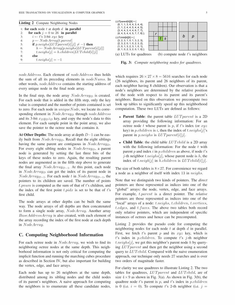
Listing 2 Compute Neighboring Nodes
1: for each node t at depth d in parallel2: for each j = 0 to 26 in parallel3: i← t’s 3-bit xyz key4: p← NodeArray[t.parent]5: if p.neighs[LUTparent[i][j]] 6= −1 then6: h← NodeArray[p.neighs[LUTparent[i][j]]]7: t.neighs[j] = h.children[LUTchild[i][j]]8: else9: t.neighs[j] = −1
nodeAddress. Each element of nodeAddress thus holds
the sum of all its preceding elements in nodeNums. In
other words, nodeAddress contains the starting address of
every unique node in the final node array.
In the final step, the node array NodeArrayD is created.
For each node that is added in the fifth step, only the key
value is computed and the number of points contained is set
to zero. For each node in uniqueNode, we locate its corre-
sponding element in NodeArrayD through nodeAddressand its 3-bit xDyDzD key, and copy the node’s data to this
element. For each sample point in the point array, we also
save the pointer to the octree node that contains it.
At Other Depths: The node array at depth D−1 can be eas-
ily built from NodeArrayD. Recall that the eight siblings
having the same parent are contiguous in NodeArrayD.
For every eight sibling nodes in NodeArrayD, a parent
node is generated by setting the last three bits of the
keys of these nodes to zero. Again, the resulting parent
nodes are augmented as in the fifth step above to generate
the final array NodeArrayD−1. At this point, each node
in NodeArrayD can get the index of its parent node in
NodeArrayD−1. For each node t in NodeArrayD−1, the
pointers to its children are saved. The number of points
t.pnum is computed as the sum of that of t’s children, and
the index of the first point t.pidx is set to be that of t’sfirst child.
The node arrays at other depths can be built the same
way. The node arrays of all depths are then concatenated
to form a single node array, NodeArray. Another array
BaseAddressArray is also created, with each element of
the array recording the index of the first node at each depth
in NodeArray.
C. Computing Neighborhood Information
For each octree node in NodeArray, we wish to find its
neighboring octree nodes at the same depth. This neigh-
borhood information is not only critical for computing the
implicit function and running the marching cubes procedure
as described in Section IV, but also important for building
the vertex, edge, and face arrays.
Each node has up to 26 neighbors at the same depth,
distributed among its sibling nodes and the child nodes
of its parent’s neighbors. A naive approach for computing
the neighbors is to enumerate all these candidate nodes,
s
r
tpb
LUTparent[4][9] = {
{0, 1, 1, 3, 4, 4, 3, 4, 4},
{1, 1, 2, 4, 4, 5, 4, 4, 5},
{3, 4, 4, 3, 4, 4, 6, 7, 7},
{4, 4, 5, 4, 4, 5, 7, 7, 8} };
LUTchild[4][9] = {
{3, 2, 3, 1, 0, 1, 3, 2, 3},
{2, 3, 2, 0, 1, 0, 2, 3, 2},
{1, 0, 1, 3, 2, 3, 1, 0, 1},
{0, 1, 0, 2, 3, 2, 0, 1, 0} };
(a) LUTs for quadtrees (b) compute node t’s neighbors
Fig. 3: Compute neighboring nodes for quadtrees.
which requires 26× 27× 8 = 5616 searches for each node
(26 neighbors, its parent and 26 neighbors of its parent,
each neighbor having 8 children). Our observation is that a
node’s neighbors are determined by the relative position
of the node with respect to its parent and its parent’s
neighbors. Based on this observation we precompute two
look up tables to significantly speed up this neighborhood
computation. These two LUTs are defined as follows:
• Parent Table: the parent table LUTparent is a 2D
array providing the following information: For an
octree node t whose parent is p, if t’s index (or xyzkey) in p.children is i, then the index of t.neighs[j]’sparent in p.neighs is LUTparent[i][j].
• Child Table: the child table LUTchild is a 2D array
with the following information: For the node t with
parent p and index i in p.children as above, if node t’sj-th neighbor t.neighs[j], whose parent node is h, the
index of t.neigh[j] in h.children is LUTchild[i][j].
The size of both tables is 8×27. For convenience we regard
a node as a neighbor of itself with index 13 in neighs.
Note that we distinguish two kinds of pointers. The direct
pointers are those represented as indices into one of the
“global” arrays: the node, vertex, edge, and face arrays.
For example, t.parent is a direct pointer. The relative
pointers are those represented as indices into one of the
“local” arrays of a node: t.neighs, t.children, t.vertices,
t.edges, and t.faces. The above two tables both record
only relative pointers, which are independent of specific
instances of octrees and hence can be precomputed.
Listing 2 provides the pseudo code for computing the
neighboring nodes for each node t at depth d in parallel.
First, we fetch t’s parent p and its xyz key, which is
t’s index in p.children. To compute t’s j-th neighbor
t.neighs[j], we get this neighbor’s parent node h by query-
ing LUTparent and then get the neighbor using a second
query to LUTchild. Compared with the naive enumeration
approach, our technique only needs 27 searches and is over
two orders of magnitude faster.
For clarity we use quadtrees to illustrate Listing 2. The two
tables for quadtrees, LUTparent and LUTchild, are of
size 4×9 as shown in Fig. 3(a). As shown in Fig. 3(b), the
quadtree node t’s parent is p, and t’s index in p.childrenis 0 (i.e. i = 0). To compute t’s 2-th neighbor (i.e. j =
IEEE TRANSACTIONS ON VISUALIZATION & COMPUTER GRAPHICS 6
2), we first get p’s 1-th neighbor, which is b, according
to LUTparent[0][2] ≡ 1. Since LUTchild[0][2] ≡ 3, b’s
3-th child, which is r, is the neighboring node we want.
Therefore, t.neighs[2] = b.children[3] = r.
To compute t’s 7-th neighbor (i.e. j = 7), we first
get p’s 4-th neighbor, which is p itself, according to
LUTparent[0][7] ≡ 4. Since LUTchild[0][7] ≡ 1, p’s
1-th child, which is s, is the node we want. Therefore,
t.neighs[7] = p.children[1] = s.
When computing a node’s neighbors, its parent’s neighbors
are required. For this reason we perform Listing 2 for all
depths using a (forward) level-order traversal of the octree.
If node t’s j-th neighbor does not exist, t.neighs[j] is set
as −1. For the root node, all its neighbors is −1 except its
13-th neighbor which is the root itself.
D. Vertex, Edge, and Face Arrays
Vertex Array: Each octree node has eight corner vertices.
Simply adding the eight vertices of every node into the
vertex array will introduce many duplications because a
corner may be shared by up to eight nodes. A simple way
to create a duplication-free vertex array is to sort all the
candidate vertices by their keys and then remove duplicate
keys, just as we did for the node array in Section III-B. This
approach, however, is inefficient due to the large number
of nodes. For example, for the Armadillo example shown
in Fig. 1, there are around 670K nodes at depth 8 and the
number of candidate vertices is over 5M. Sorting such a
large array takes over 100ms.
We present a more efficient way to create the vertex
array by making use of node neighbors computed in
Section III-C. Building the vertex array at octree depth dtakes the following steps. First, we find in parallel a unique
owner node for every corner vertex. The owner node of a
corner is defined as the node that has the smallest shuffled
xyz key among all nodes sharing the corner. Observing
that all nodes that share corners with node t must be t’sneighbors, we can quickly locate the owner of each corner
from t’s neighbors. Second, for each node t in parallel, all
corner vertices whose owner is t itself are collected. The
unique vertex array is then created. During this process,
the vertex pointers t.vertices are saved. For each vertex
v in the vertex array, the node pointers v.nodes are also
appropriately set.
To build the vertex array of all octree nodes, the above
process is performed at each depth independently, and
the resulting vertex arrays are concatenated to form a
single vertex array. Unlike the node array, the vertex array
so obtained still has duplicate vertices between different
depths. However, since this does not affect our subsequent
surface reconstruction, we leave these duplicate vertices as
they are in our current implementation.
Other Arrays: The edge and face arrays can be built in a
similar way. For each edge/face of each node, we first find
its owner node. Then the unique edge/face array is created
by collecting edges/faces from the owner nodes.
IV. GPU Surface Reconstruction
In this section we describe how to reconstruct surfaces
from sample points using the octree constructed in the last
section. The reconstruction roughly consists of two steps.
First, an implicit function ϕ over the volume spanned by
the octree nodes is computed using Poisson surface recon-
struction [2]. Then, an adaptive marching cubes procedure
extracts a watertight mesh as an isosurface of the implicit
function.
Note that, instead of Poisson surface reconstruction, we
may use other methods (e.g. [3] and [13]) for GPU surface
reconstruction. We chose the Poisson approach because it
can reconstruct high quality surfaces through a global op-
timization. In addition, the Poisson approach only requires
solving a well-conditioned sparse linear system, which can
be efficiently done on the GPU.
Specifically, we perform the following steps on the GPU:
1) Build a linear system Lx = b, where L is the
Laplacian matrix and b is the divergence vector;
2) Solve the above linear system using a multigrid
solver,
3) Compute the isovalue as an average of the implicit
function values at sample points,
4) Extract the isosurface using marching cubes.
The mathematical details of Poisson surface reconstruction
(Step 1 and 2) are reviewed in Appendix. In the following,
we describe the GPU procedures for these steps.
A. Computing Laplacian Matrix L
As described in Appendix, the implicit function ϕ is a
weighted linear combination of a set of blending functions
{Fo} with each function Fo corresponding to a node of
the octree. An entry of the Laplacian matrix Lo,o′ =〈Fo,∆Fo′〉 is the inner product of blending function Fo
and the Laplacian of Fo′ .
The blending function Fo is given by a fixed basis function
F :
Fo(q) = F
(
q − o.c
o.w
)
1
o.w3, (1)
where o.c and o.w are the center and width of the octree
node o. F is non-zero only inside the cube [−1, 1]3. As
explained in Appendix, F is a separable function of x, yand z. As a result, the blending function Fo is separable as
well and can be expressed as:
Fo(x, y, z) = fo.x,o.w(x)fo.y,o.w(y)fo.z,o.w(z).
Given the definition of Laplacian ∆Fo′ = ∂2Fo′
∂x2 + ∂2Fo′
∂y2 +∂2F
o′
∂z2 , the Laplacian matrix entry Lo,o′ can be computed

IEEE TRANSACTIONS ON VISUALIZATION & COMPUTER GRAPHICS 7
Listing 3 Compute Divergence Vector b
1: // Step 1: compute vector field2: for each node o at depth D in parallel3: ~vo = 04: for j = 0 to 265: t← NodeArray[o.neighs[j]]6: for k = 0 to t.pnum7: i = t.pidx + k8: ~vo + = ~niFqi,o.w(o.c)
9: // Step 2: compute divergence for finer depth nodes10: for d = D to 511: for each node o at depth d in parallel12: bo = 013: for j = 0 to 2614: t← NodeArray[o.neighs[j]]15: for k = 0 to t.dnum16: idx = t.didx + k17: o′ ← NodeArray[idx]18: bo + = ~vo′~uo,o′
19: // Step 3: compute divergence for coarser depth nodes20: for d = 4 to 021: divg ← new array22: for node o at depth d23: for each depth-D node o′ covered by all nodes in
o.neighs in parallel24: divg[i] = ~vo′~uo,o′
25: bo = Reduce(divg, +)
as:
Lo,o′ =
⟨
Fo,∂2Fo′
∂x2
⟩
+
⟨
Fo,∂2Fo′
∂y2
⟩
+
⟨
Fo,∂2Fo′
∂z2
⟩
=
〈fo.x,o.w, f′′
o′.x,o′.w〉〈fo.y,o.w, fo′.y,o′.w〉〈fo.z,o.w, fo′.z,o′.w〉+
〈fo.x,o.w, fo′.x,o′.w〉〈fo.y,o.w, f′′
o′.y,o′.w〉〈fo.z,o.w, fo′.z,o′.w〉+
〈fo.x,o.w, fo′.x,o′.w〉〈fo.y,o.w, fo′.y,o′.w〉〈fo.z,o.w, f′′
o′.z,o′.w〉.
All the above inner products can be efficiently computed
by looking up two precomputed 2D tables: one for 〈fo, fo′〉and the other for 〈fo, f
′′o′〉. These two tables are queried
using the x-bits, y-bits, or z-bits of the shuffled xyz keys of
node o and o′. This reduces the table size significantly. For a
maximal octree depth 9, the table size is (210−1)×(210−1).The table size may be further reduced because the entries
of the tables are symmetric.
B. Evaluating Divergence Vector b
As described in Appendix, the divergence coefficients bo
can be computed as:
bo =∑
o′∈OD~vo′ · ~uo,o′ ,
where ~uo,o′ = 〈Fo(q),∇Fo′〉. OD is the set of all octree
nodes at depth D. The inner product 〈Fo(q),∇Fo′〉 can be
quickly computed using a precomputed look up table for
〈fo, f′o′〉 as in the computation of Lo,o′ . As for ~vo′ , it is
computed as
~vo′ =∑
qi∈Qαo′,qi
~ni, (2)
where αo,qiis the weight by which each sampling point qi
distributes the normal ~ni to its eight closest octree nodes
at depth D.
Listing 4 Compute Implicit Function Value ϕq for Point q
1: ϕq = 02: nodestack ← new stack3: nodestack.push(proot)4: while nodestack is not empty5: o← NodeArray[nodestack.pop()]6: ϕq+ = Fo(q)ϕo
7: for i = 0 to 78: t← NodeArray[o.children[i]]9: if q.x− t.x < t.w and q.y− t.y < t.w and q.z− t.z <
t.w then10: nodestack.push(o.children[i])
Listing 3 provides the pseudo code for computing the
divergence vector b. This computation takes three steps.
In the first step, the vector field ~vo′ is computed for each
octree node o′ according to Eq. (2). Since Eq. (2) essentially
distributes sample point qi’s normal ~ni to its eight nearest
octree nodes at depth D, vector ~vo′ is only affected by the
sample points that are contained in either node o′ or its 26
neighbors. The pointers to the node neighbors as recorded
in Section III-C are used to locate these neighbors.
In the second step, the divergence at every finer depth,
which is defined as any depth greater than four, is computed
in parallel for all nodes, as shown in Step 2 of Listing 3. The
most obvious way to accumulate bo for each octree node
o is to iterate through all nodes o′ at depth D. However,
this costly full iteration is actually not necessary. Since the
basis function F ’s domain of support is the cube [−1, 1]3,
~uo,o′ equals zero for a large number node pairs (o, o′).Specifically, we can easily prove that, for node o, only
the depth-D nodes whose ancestors are either o or o’s
neighbors have nonzero ~uo,o′ . These nodes can be located
by iterating over o’s neighbors. Note that t.dnum and
t.didx are the number of depth-D nodes covered by t and
the pointer to t’s first depth-D node respectively. These
information can be easily obtained and recorded during tree
construction.
In the third step, the divergence at every coarser depth,
which is defined as any depth no greater than four, is
computed. For nodes at a coarser depth, the approach taken
in the second step is not appropriate because it cannot
exploit the fine-grained parallelism of GPUs. The node
number at coarser depths is much smaller than that at finer
depths, and the divergence of a node at a coarser depth may
be affected by many depth-D nodes. For example, at depth
zero, there is only one root node and all depth-D nodes
contribute to its divergence. To maximize parallelism, we
parallelize the computation over all covered depth-D nodes
for nodes at coarser depths. As shown in Step 3 of Listing 3,
we first compute the divergence contribution for each depth-
D node in parallel and then perform a reduction operation
to sum up all contributions.
C. Multigrid Solver and Implicit Function
The GPU multigrid solver is rather straightforward. For
each depth d from coarse to fine, the linear system Ldx
d =

IEEE TRANSACTIONS ON VISUALIZATION & COMPUTER GRAPHICS 8
bd is solved using a conjugate gradient solver for sparse
matrices [33]. Ld contains as many as 27 nonzero entries
in a row. For each row, the values and column indices
of nonzero entries are stored in a fixed-sized array. The
number of the nonzero entries is also recorded.
Note that the divergence coefficients at depth d need to
be updated using solutions at coarser depths according to
Eq. (6) in Appendix. For the blending function Fo of an
arbitrary octree node o, it can be easily shown that only the
blending functions of o’s ancestors and their 26 neighbors
may overlap with Fo. Therefore, we only need to visit these
nodes through the pointers stored in parent and neighsfields of node o.
To evaluate the implicit function value at an arbitrary point
q in the volume, we need to traverse the octree. Listing 4
shows the pseudo code of a depth-first traversal for this
purpose. A stack is used to store the pointers to all nodes
to be traversed. For this traversal, a stack size of 8D is
enough for octrees with a maximal depth D.
Note that the implicit function value of a sample point
qi can be evaluated in a more efficient way, because we
already know the depth-D node o where qi is located. In
other words, we only need to traverse octree nodes whose
blending function may overlap with that of o. These nodes
include o itself, o’s neighbors, o’s ancestors, and the neigh-
bors of o’s ancestors. Once we get the implicit function
values at all sample points, the isovalue is computed as an
average: ϕ =∑
i ϕ(qi)/N . A point is deemed to be outside
the surface being reconstructed if its implicit function value
is greater than ϕ.
D. Isosurface Extraction
We use the marching cubes technique [34] on the leaf nodes
of the octree to extract the isosurface. The output is a vertex
array and a triangle array which can be rendered directly.
As shown in Listing 5, the depth-D nodes are processed in
five steps. First, the implicit function values are computed
for all octree vertices in parallel. As in the case with
the sample points, each vertex v’s implicit function value
can be efficiently computed by traversing only the related
nodes, which can be located through the pointers stored in
v.nodes. Second, the number of output vertices is computed
with a single pass over the octree edges and the output
address is computed by performing a scan operation. Third,
each node’s cube category is calculated and the number
and addresses of output triangles are computed. Finally, in
Step 4 and 5 the vertices and triangles are generated and
saved. During this process, for each face of each node, if
one of its four edges has a surface-edge intersection, the
face is deemed to contain surface-edge intersections and we
mark the face. This information is propagated to the node’s
ancestors.
For all leaf nodes at other depths, we first filter out nodes
that do not produce triangles in parallel. For each node, if
Listing 5 Marching Cubes
1: // Step 1: compute implicit function values for octree vertices2: vvalue← new array3: for each octree vertex i at depth-D in parallel4: Compute the implicit function value vvalue[i]5: vvalue[i] − = ϕ
6: // Step 2: compute vertex number and address7: vexNums← new array8: vexAddress← new array9: for each edge i at depth-D in parallel
10: if the values of i’s two vertices have different sign then11: vexNums[i] = 112: else13: vexNums[i] = 014: Scan(vexAddress, vexNums, +)
15: // Step 3: compute triangle number and address16: triNums← new array17: triAddress← new array18: for each node i at depth-D in parallel19: Compute the cube category based the values of i’s vertices20: Compute triNums[i] according to the cube category21: Scan(triAddress, triNums, +)
22: // Step 4: generate vertices23: Create V ertexBuffer according to vexAddress24: for each edge i at depth-D in parallel25: if vexNums[i] == 1 then26: Compute the surface-edge intersection point q27: V ertexBuffer[vexAddress[i]] = q
28: // Step 5: generate triangles29: Create TriangleBuffer according to triAddress30: for each node i at depth-D in parallel31: Generate triangles based on the cube category32: Save triangles to TriangleBuffer[triAddress[i]]
the implicit function values at its eight corners have the
same sign and none of its six faces contain surface-edge
intersections, the node does not need any further processing.
Otherwise, we subdivide the node to depth D. All the
depth-D nodes generated by this subdivision are collected
to build the new node, vertex and edge arrays. Then, we
perform Listing 5 to generate vertices and triangles. This
procedure is carried out iteratively until no new triangles
are produced. Note that in each iteration, we do not need
to handle the nodes subdivided in previous iterations.
Finally, to remove duplicate surface vertices and merge
vertices located closely to each other, we compute the
shuffled xyz key for each vertex and use the keys to
sort all vertices. Vertices having the same key values are
merged by performing a parallel compact operation. The
elements in the triangle array are updated accordingly
and all degenerated triangles are removed. Each triangle’s
normal is also computed.
Discussion: Besides the Poisson method, we can also
design GPU algorithms for other implicit reconstruction
methods. For example, an early technique [3] calculates a
signed distance field and reconstructs a surface by extract-
ing the zero set of the distance field using the marching
cubes. With the octrees we construct, the distance field can

IEEE TRANSACTIONS ON VISUALIZATION & COMPUTER GRAPHICS 9
Model # Points Tree Depth # Triangles Memot Mem Tot Tfunc Tiso Ttotal FPS Totcpu Tcpu
Bunny 353272 8 228653 120MB 290MB 40ms 144ms 6ms 190ms 5.26 8.5s 39s
Buddha 640735 8 242799 160MB 320MB 50ms 167ms 35ms 252ms 3.97 16.1s 38s
Armadillo 512802 8 201340 140MB 288MB 43ms 149ms 5ms 197ms 5.06 12.8s 42s
Elephant 216643 8 142197 200MB 391MB 46ms 209ms 41ms 296ms 3.38 5.5s 34s
Hand 259560 8 184747 125MB 253MB 36ms 143ms 27ms 206ms 4.85 6.4s 26s
Dragon 1565886 9 383985 230MB 460MB 251ms 486ms 23ms 760ms 1.31 39.1s 103s
TABLE I: Running time and memory performance for some examples shown in the paper. # Triangles is the number
of triangles in the reconstructed surface. Memot is the memory consumed by the octree data structure only, and Mem
is the total memory consumed by the whole algorithm. Tot, Tfunc, Tiso and Ttotal are the time for building octree,
implicit function computation (including both linear system building and solving), isosurface extraction and total time
respectively, using our GPU algorithm. FPS is the frame rates of our algorithm. For comparison, T otcpu and Tcpu are the
octree building time and total time using the CPU algorithm [2].
be quickly estimated on the GPU: processing each octree
vertex in parallel, we locate its nearest sample point by
traversing the octree using a procedure similar to that shown
in Listing 4 and compute the signed distance between the
vertex and a plane defined by the position and normal of this
sample point. Then our adaptive marching cubes procedure
is applied to extract the zero set surface. As noted in [2],
the quality of surfaces reconstructed this way is not as good
as those produced by the Poisson method.
V. Results and Applications
We have implemented the described surface reconstruction
algorithm on an Intel Xeon 3.7GHz CPU with a GeForce
8800 ULTRA (768MB) graphics card.
Implementation Details: The G80 GPU is a highly parallel
processor working on many threads simultaneously. CUDA
structures GPU programs into parallel thread blocks of up
to 512 parallel threads. We need to specify the number of
thread blocks and threads per block for GPU programs,
i.e. the parallel primitives (e.g. Sort, Compact and
Scan) and the programs marked in parallel. In our current
implementation, we use 256 threads for each block. The
block number is computed by dividing the total number
of parallel processes by the thread number per block. For
example, in Step 2 (line 5) of Listing 1, the block number
is N/256.
The whole octree data and multigrid solver data are stored
in the global memory/texture memory. They are too huge
to be stored in the shared memory, which is mainly used
in GPU primitives such as sort, compact and scan. For
these primitives, we used the implementation provided
in CUDPP [31], which is well optimized in terms of
coalescent memory access. Since most computations in our
algorithm map to these primitives, our algorithm is well
optimized. The LUTs are also stored in the shared memory.
Reconstruction Results: We tested our algorithm on a
variety of real-world scan data. As a preprocess, normals
are computed using Stanford’s Scanalyze system. As shown
in Fig. 1, our GPU algorithm is capable of generating high
quality surfaces with fine details from noisy real-world
scans, just like the CPU algorithm in [2].
In terms of performance, the GPU algorithm is over two
orders of magnitude faster than the CPU algorithm. For
example, for the Stanford Bunny, the GPU algorithm runs
at 5.2 frames per second, whereas the CPU algorithm
takes 39 seconds for a single frame. Note that the CPU
implementation is provided by the authors of [2] and is
well optimized.
As summarized in TABLE I, the GPU algorithm achieves
interactive performance for all examples shown in the pa-
per. Currently, the implicit function computation, especially
the stage of building the linear system, is the bottleneck of
our algorithm. The time for octree construction occupies
a relatively small fraction. Compared with the CPU octree
construction algorithm, our GPU octree builder is also over
two orders of magnitude faster.
Note that the Dragon model in TABLE I contains some
noisy points that distribute far away from the dragon body.
So its bounding box is not fit tightly to the dragon body.
This leads to the result that the number of output triangles
at level 9 is about 460K, comparable to those numbers
reported in [2].
Limitation: The memory consumption of our algorithm is
dominated by the octree depth as is the case with CPU
reconstruction algorithms. As a result, our GPU reconstruc-
tion can only handle octrees with a maximal depth of 9due to the limited memory of our current graphics card.
On the other hand, since the memory consumption is not
dominated by the input point cloud size, our algorithm can
handle large input point clouds. For example, the algorithm
can handle only 2000K points at octree depth 9. But at
octree depth 8, the algorithm can handle up to 5000K points
(consumes around 600MB memory, runs at around 2 frames
per second). Our ability to handle large input also increases
with the rapid improvements in graphics hardware (e.g.
Quadro FX 5600 released by NVIDIA supports CUDA and
has 1.5GB memory). Nevertheless, with the advent of 3D
scanners, scanned models are likely to contain too many
points to be handled by any GPU and CPU method. There
is a need to develop out-of-core methods on GPUs as well
as on CPUs. This is beyond the scope of this paper and left
to future work.

IEEE TRANSACTIONS ON VISUALIZATION & COMPUTER GRAPHICS 10
(a) (b)
(c) (d)
Fig. 4: User-guided reconstruction of a scanned elephant
model. (a) The input scan. (b) The result from automatic
reconstruction. The head and trunk are mistakenly con-
nected. (c) The improved surface after the user draws the
stroke shown in (b). (d) A tail copied from the Armadillo is
added around the rear end of the elephant. A new elephant
surface with the new tail is immediately reconstructed. See
the companion video for live demos.
A. User-Guided Surface Reconstruction
Using our GPU reconstruction technique, we develop a
user-guided surface reconstruction algorithm for imperfect
scan data. The algorithm allows the user to draw strokes
to reduce topological ambiguities in areas that are under-
sampled or completely missing in the input data. Since our
GPU reconstruction technique is interactive, the user can
view the reconstructed surface immediately after drawing
a stroke. Compared with a previous user-assisted method
[4] which takes several minutes to update the reconstructed
mesh, our approach is more effective and provides better
user experience.
Our basic idea is to first add new oriented sample points to
the original point cloud based on user interaction. Then a
new isosurface is generated for the augmented point cloud.
Suppose Q is the original point set and Q′ is the current
point set after each user interaction. After the user draws
a stroke, our system takes the following steps to generate
the new surface:
1) Compute the depth range of Q’s bounding box under
the current view.
2) Iteratively extrude the stroke along the current view
direction in the depth range, with a user-specified
interval w. For each extruded stroke, a set of points
are uniformly distributed along the stroke, also with
interval w. Denote this point set as S.
3) For points in S, compute their implicit function
values in parallel using the procedure in Listing 4.
4) Remove points from S whose implicit function values
are not less than the current isovalue ϕ.
5) Compute normals for all points in S.
Fig. 5: User-guided reconstruction of a scanned hand
model. Left: the automatic reconstruction result. Several
fingers are mistakenly connected. Right: the improved sur-
face after the user draws two rectangles.
6) Add S to the current point set Q′.
7) Perform GPU reconstruction with Q′ as input and
generate the new isosurface.
In Step 2, the interval w is set to be the width of an
octree node at depth D by default. Step 4 removes points
outside of the current reconstructed surface because we only
wish to add new points in inner regions, where topological
ambiguity is found. This scheme works well for all tested
data shown in this paper. Note that unwanted points may
be accidentally introduced in some inner regions. When
this happens, the user can remove those points manually. In
Step 7, the new isovalue is always computed as the average
of the implicit function values of points in the original point
set Q because we want to restrict the influence of newly-
added points to local areas. The new points are only used
to change the local vector field.
Our current system provides two ways to compute the
normals for points in S in Step 5. One is based on normal
interpolation. For each point si ∈ S, we traverse the octree
of Q′ and find all points of Q′ which are enclosed by a
box centered at si. Then si’s normal is computed as an
interpolation of the normals of these points. The interpola-
tion weight of a point q′ is proportional to the reciprocal
of the squared distance between q′ and si. The box size is
a user-specified parameter. If no point is found given the
current box size, the algorithm automatically increases the
box size and traverses the octree again. The other scheme
for computing the normals is relatively simple. The normals
are restricted to be orthogonal to both the current viewing
direction and the tangents of the stroke. We always let the
normals point to the right side of the stroke.
Note that for the first normal computation scheme, the
user’s interaction is not limited to drawing strokes. We also
allow users to draw a rectangle or any closed shape to define
an area where they want to insert new points. This shape is
then extruded along the current view direction in the depth
range to form a volume and a set of points is uniformly
distributed inside the volume. After that, Steps 3 ∼ 7 are
performed to generate a new isosurface.

IEEE TRANSACTIONS ON VISUALIZATION & COMPUTER GRAPHICS 11
Fig. 6: Free form deformation and boolean operations.
Top left: several tentacles are pulled out from an ellip-
soid. Bottom left: a hole and a face mask are created
on the bunny’s surface. Right: an interesting creature is
created from the armadillo using free-form deformation and
boolean operations.
User-Guided Reconstruction Results: We tested our al-
gorithm on a variety of complex objects including the
Buddha (Fig. 1), Elephant (Fig. 4), and Hand (Fig. 5).
For all examples, we were able to generate satisfactory
results after several strokes. See the companion video for
examples of user interaction sessions. While the user-
specified inside/outside constraints in [4] only correct the
local topology, our system also allows the user to specify
the geometry of missing areas of the surface. The user first
copies a set of points from another point cloud and places
the points around the target area. The new isosurface can be
then generated. Note that in this case, we do not remove the
points outside of the surface as in Step 4 above. Fig. 4(d)
shows such an example.
B. On-the-fly Conversion of Dynamic Point
Clouds
Our GPU reconstruction algorithm can also be integrated
into point cloud modeling tools to generate meshes for
dynamic point clouds on the fly. The reconstructed meshes
can be directly rendered using conventional polygon-based
rendering methods.
Free-Form Deformation: We first implemented the free-
form deformation tool described in [35]. The GPU recon-
struction is performed on the deformed point cloud at each
frame to produce a triangular mesh. As shown in Fig. 6 and
the companion video, our system is capable of generating
high quality surfaces at interactive frame rates, even as
dynamic sampling is enabled.
Boolean Operations: Suppose Q1 and Q2 are two point
clouds. First, two implicit functions (ϕ1 and ϕ2) are
computed for Q1 and Q2 respectively and two isosur-
faces M1 and M2 are extracted. Second, for each point
qi2∈ Q2 in parallel, the implicit function value ϕ1(q
i2) is
Fig. 7: Real-time fluid surface reconstruction. Left: parti-
cles. Right: the reconstructed surface.
computed using the pseudo code in Listing 4. Similarly,
for each point qi1∈ Q1, ϕ2(q
i1) is computed. Third, the
inside/outside classification is done by comparing each
ϕ1(qi2) with ϕ1, and each ϕ2(q
i1) with ϕ2. Fourth, based
on the inside/outside classification, a new point cloud Q is
produced by collecting points from Q1 and Q2 according
to the definition of the specific Boolean operation being
performed. Finally, GPU reconstruction is performed on Qto generate a surface for the Boolean operation.
Fig. 6 shows some results generated using our algorithm.
Please refer to the companion video for interactive demos.
Note that these point cloud editing examples are simply
used to demonstrate on-the-fly conversion of dynamic point
clouds to polygonal models, a new capability enabled by
our GPU surface reconstruction. The point cloud editing
operations are performed with existing techniques, not new
techniques.
C. Real-time Fluid Surface Reconstruction
Particle-based fluid simulation techniques have been able
to achieve real-time performance and are widely used in
interactive applications [36]. The simulation output is a set
of 3D particles. Although point splatting can be used to
render the fluid surface, it is still necessary to extract an
isosurface to get high quality rendering effects as noted in
[36]. Our GPU reconstruction can be used to reconstruct
fluid surfaces in real time.
We implemented a fluid surface reconstruction algorithm in
the particle demo provided in NVIDIA CUDA SDK. Taking
the particle positions as input, the algorithm first builds an
octree which is used to quickly find the nearby particles for
each particle. Then, the implicit function over the space of
the octree is computed using the method proposed by Zhu
and Bridson [37]. Finally the isosurface is extracted as in
Section 5 and directly rendered. Note that the algorithm
in [37] needs a range search process to find the nearby
particles for each particle. This can be efficiently performed
using a procedure similar to Listing 4.
Fig. 7 shows a static frame of the simulation result. For 32K
particles, the simulation procedure alone runs at around
240 fps. With our fluid surface reconstruction at octree
depth 6, the whole program runs at about 50 fps. The
reconstructed surface is directly shaded on the GPU. The

IEEE TRANSACTIONS ON VISUALIZATION & COMPUTER GRAPHICS 12
program also allows users to interact with the fluid. Please
see the companion video for interactive demos.
VI. Conclusion and Future Work
We have presented a parallel surface reconstruction al-
gorithm that runs entirely on the GPU. For moderate-
sized scan data, this GPU algorithm generates high quality
surfaces with fine details at interactive frame rates, which
is over two orders of magnitude faster than CPU algo-
rithms. We believe that our contribution is not limited to a
GPU implementation of the Poisson reconstruction method,
but a general approach for designing GPU algorithms
for highly parallel surface reconstruction. As described
in Section IV-D, GPU algorithms for other reconstruction
techniques such as the classic technique in [3] can be easily
designed following our approach. It is also important to
note that since octrees are ubiquitous in computer graphics,
our GPU octree construction technique, which is a core
component of our approach, can have impact in many
applications beyond surface reconstruction. One example
is octree texture painting [38].
Our GPU reconstruction algorithm not only enhances ex-
isting applications but also opens up new possibilities.
To demonstrate its potential, we integrate the algorithm
into a user-guided reconstruction system for imperfect scan
data and thus enable interactive reconstruction according to
user input. We also show how to employ the algorithm
in point cloud modeling tools for generating polygonal
surfaces from dynamic point clouds on the fly as well as
to reconstruct fluid surfaces in real time.
For future work, we are interested in exploring the scenario
with unreliable normals given at the sample points. In
this case, a possible approach is to use the inside/outside
constraints [4] instead of normal constraints in implicit
function optimization. We are also interested in enhancing
our user-guided surface reconstruction by developing an
automatic method for detecting problematic regions as in
[4]. Such a method will save the user the trouble of having
to locate these topologically unstable regions.
Acknowledgements
We would like to thank Andrei Sharf and Daniel Cohen-
Or for providing the scan data of Elephant and Hand, and
Steve Lin for video dubbing. This research was partially
funded by the NSFC (No. 60825201) and the 973 program
of China (No. 2009CB320801). .
References
[1] NVIDIA, “CUDA programming guide 2.0,” 2008,http://developer.nvidia.com/object/cuda.html.
[2] M. Kazhdan, M. Bolitho, and H. Hoppe, “Poisson surface recon-struction,” in SGP’06, 2006, pp. 61–70.
[3] H. Hoppe, T. DeRose, T. Duchamp, J. McDonald, and W. Stuet-zle, “Surface reconstruction from unorganized points,” in SIG-
GRAPH’92, 1992, pp. 71–78.
[4] A. Sharf, T. Lewiner, G. Shklarski, S. Toledo, and D. Cohen-Or, “In-teractive topology-aware surface reconstruction,” ACM Transactions
on Graphics, vol. 26, no. 3, pp. 43, 9, 2007.
[5] J.-D. Boissonnat, “Geometric structures for three-dimensional shaperepresentation,” ACM Transactions on Graphics, vol. 3, no. 4, pp.266–286, 1984.
[6] N. Amenta, M. Bern, and M. Kamvysselis, “A new Voronoi-basedsurface reconstruction algorithm,” in SIGGRAPH’98, 1998, pp. 415–421.
[7] C. L. Bajaj, F. Bernardini, and G. Xu, “Automatic reconstruction ofsurfaces and scalar fields from 3d scans,” in SIGGRAPH’95, 1995,pp. 109–118.
[8] R. Kolluri, J. R. Shewchuk, and J. F. O’Brien, “Spectral surfacereconstruction from noisy point clouds,” in SGP’04, 2004, pp. 11–21.
[9] B. Curless and M. Levoy, “A volumetric method for buildingcomplex models from range images,” in SIGGRAPH’96, 1996, pp.302–312.
[10] A. Hornung and L. Kobbelt, “Robust reconstruction of watertight 3dmodels from non-uniformly sampled point clouds without normalinformation,” in SGP’06, 2006, pp. 41–50.
[11] J. C. Carr, R. K. Beatson, J. B. Cherrie, T. J. Mitchell, W. R. Fright,B. C. McCallum, and T. R. Evans, “Reconstruction and represen-tation of 3d objects with radial basis functions,” in SIGGRAPH’01,2001, pp. 67–76.
[12] G. Turk and J. F. O’Brien, “Modelling with implicit surfaces thatinterpolate,” ACM Transactions on Graphics, vol. 21, no. 4, pp. 855–873, 2002.
[13] Y. Ohtake, A. Belyaev, M. Alexa, G. Turk, and H.-P. Seidel, “Multi-level partition of unity implicits,” ACM Transactions on Graphics,vol. 22, no. 3, pp. 463–470, 2003.
[14] M. Alexa, J. Behr, D. Cohen-Or, S. Fleishman, D. Levin, and C. T.Silva, “Point set surfaces,” in IEEE Visualization’01, 2001, pp. 21–28.
[15] N. Amenta and Y. J. Kil, “Defining point-set surfaces,” ACM
Transactions on Graphics, vol. 22, no. 3, pp. 264–270, 2004.
[16] Y. Lipman, D. Cohen-Or, and D. Levin, “Data-dependent MLS forfaithful surface approximation,” in SGP’07, 2007, pp. 59–67.
[17] M. Randrianarivony and G. Brunnett, “Parallel implementationof surface reconstruction from noisy samples. Preprint Sonder-forschungsbereich 393, SFB 393/02-16,” 2002.
[18] N. A. Borghese, S. Ferrari, and V. Piuri, “Real-time surface recon-struction through HRBF networks,” in IEEE International Workshop
on Haptic Virtual Environments and Their Applications, 2002, pp.19–24.
[19] K. Weinert, T. Surmann, and J. Mehnen, “Parallel surface reconstruc-tion,” in Proceedings of the 5th European Conference on Genetic
Programming, 2002, pp. 93–102.
[20] C. Buchart, D. Borro, and A. Amundarain, “GPU local triangula-tion: an interpolating surface reconstruction algorithm,” Computer
Graphics Forum, vol. 27, no. 3, 2008.
[21] M. Gopi, S. Krishnan, and C. Silva, “Surface reconstruction basedon lower dimensional localized Delaunay triangulation,” in Euro-
graphics’00, 2000, pp. 467–478.
[22] Y. J. Kil and N. Amenta, “GPU-assisted surface reconstruction onlocally-uniform samples,” Tech. Rep., UC, Davis, CSE-2008-8 2008.
[23] J. Wilhelms and A. V. Gelder, “Octrees for faster isosurface genera-tion,” ACM Transactions on Graphics, vol. 11, no. 3, pp. 201–227,1992.

IEEE TRANSACTIONS ON VISUALIZATION & COMPUTER GRAPHICS 13
[24] R. Westermann, L. Kobbelt, and T. Ertl, “Real-time exploration ofregular volume data by adaptive reconstruction of isosurfaces,” The
Visual Computer, vol. 15, no. 2, pp. 100–111, 1999.
[25] A. E. Lefohn, S. Sengupta, J. Kniss, R. Strzodka, and J. D. Owens,“Glift: Generic, efficient, random-access GPU data structures,” ACM
Transactions on Graphics, vol. 25, no. 1, pp. 60–99, 2006.
[26] C. DeCoro and N. Tatarchuk, “Real-time mesh simplification usingthe gpu,” in I3D’07, 2007, pp. 161–166.
[27] X. Sun, K. Zhou, E. Stollnitz, J. Shi, and B. Guo, “Interactiverelighting of dynamic refractive objects,” ACM Transactions on
Graphics, vol. 27, no. 3, p. 35, 2008.
[28] K. Zhou, Q. Hou, R. Wang, and B. Guo, “Real-time kd-treeconstruction on graphics hardware,” ACM Transactions on Graphics,vol. 27, no. 5, p. 126, 2008.
[29] C. Lauterbach, M. Garland, S. Sengupta, D. Luebke, andD. Manocha1, “Fast BVH construction on GPUs,” Computer Graph-
ics Forum, vol. 28, no. 2, pp. 375–384, 2009.
[30] S. Popov, J. Gunther, H.-P. Seidel, and P. Slusallek, “Stackless kd-tree traversal for high performance GPU ray tracing,” in Eurograph-
ics’07, 2007, pp. 415–424.
[31] M. Harris, J. Owens, S. Sengupta, Y. Zhang, and A. Davidson,“CUDPP homepage,” 2007, http://www.gpgpu.org/developer/cudpp/.
[32] M. Harris, S. Sengupta, and J. Owens, “Parallel prefix sum (scan) inCUDA,” in GPU Gems 3, H. Nguyen, Ed. Addison Wesley, 2007,p. Ch.31.
[33] J. Bolz, I. Farmer, E. Grinspun, and P. Schroder, “Sparse matrixsolvers on the GPU: conjugate gradients and multigrid,” ACM
Transactions on Graphics, vol. 22, no. 3, pp. 917–924, 2003.
[34] W. E. Lorensen and H. E. Cline, “Marching cubes: A high resolution3d surface construction algorithm,” in SIGGRAPH’87, 1987, pp.163–169.
[35] M. Pauly, R. Keiser, L. P. Kobbelt, and M. Gross, “Shape modelingwith point-sampled geometry,” ACM Transactions on Graphics,vol. 22, no. 3, pp. 641–650, 2003.
[36] M. Muller, D. Charypar, and M. Gross, “Particle-based fluid simu-lation for interactive applications,” in SCA’03, 2003, pp. 154–159.
[37] Y. Zhu and R. Bridson, “Animating sand as a fluid,” ACM Transac-
tions on Graphics, vol. 24, no. 3, pp. 965–972, 2005.
[38] D. Benson and J. Davis, “Octree textures,” ACM Transactions on
Graphics, vol. 21, no. 3, pp. 785–790, 2002.
Appendix
Given an input point cloud Q with each sample point qi
having a normal vector ~ni, the Poisson surface reconstruc-
tion technique [2] computes an implicit function ϕ whose
gradient best approximates a vector field ~V defined by the
samples, i.e., minϕ ‖∇ϕ− ~V ‖. This minimization problem
can be restated as solving the following Poisson equation:
∆ϕ = ∇ · ~V ,
i.e., compute a scalar function ϕ whose Laplacian (di-
vergence of gradient) equals the divergence of ~V . The
algorithm first defines a set of blending functions based on
octree O. For every node o ∈ O, a blending function Fo is
defined by centering and stretching a fixed basis function
F :
Fo(q) ≡ Fo.c,o.w(q) = F
(
q − o.c
o.w
)
1
o.w3, (3)
where o.c and o.w are the center and width of node o.
The vector field ~V is then defined as:
~V (q) ≡∑
qi∈Q
∑
o∈OD
αo,qiFo(q)~ni =
∑
o∈OD
~voFo(q), (4)
where OD are the octree nodes at depth D, αo,qiis the
trilinear interpolation weight. Each sample point qi only
distributes its normal to its eight closest octree nodes at
depth D. This works well for all scan data we tested,
although it is preferable to also “splat” the samples into
nodes at other depths for non-uniformly distributed point
samples.
The implicit function ϕ is also expressed in the function
space spanned by {Fo}:
ϕ(q) =∑
o∈O
ϕoFo(q). (5)
The Poisson equation thus reduces to a sparse linear system:
Lx = b, (6)
where x = {ϕo} and b = {bo} are |O|-dimensional
vectors. The Laplacian matrix entries are the inner products
Lo,o′ = 〈Fo,∆Fo′〉, and the divergence coefficients are
bo =∑
o′∈OD
〈Fo,∇ · (~vo′Fo′)〉 =∑
o′∈OD
〈Fo, (~vo′ · ∇Fo′)〉
=∑
o′∈OD
∫
Fo(q)(~vo′ · ∇Fo′(q))dq =∑
o′∈OD
~vo′ · ~uo,o′ ,
where ~uo,o′ =∫
Fo(q)∇Fo′(q)dq.
The linear system can be transformed into successive linear
systems
Ldx
d = bd, (7)
one per octree depth d. Since Ld is symmetric and positive
definite, each linear system can be solved using a conjugate
gradient solver. The divergence at finer depths is updated
as:
bdo ← bd
o −∑
d′<d
∑
o′∈Od′
Lo,o′ϕo′ , (8)
where Od is the set of octree nodes at depth d.
The basis function F used in [2] is the n-th convolution of
a box filter with itself:
F (x, y, z) ≡ (B(x)B(y)B(z))∗n, B(t) =
{
1, if |t| < 0.5;0, otherwise.
(9)
Kazhdan et al. used n = 3 in their implementation. In our
implementation we choose n = 2 instead. This reduces
the support of F to the domain [−1, 1]3 without noticeable
degradation of the reconstructed surfaces. Note that F is a
separable function and can be expressed as:
F (x, y, z) = f(x)f(y)f(z), (10)
where f is the n-th convolution of B with itself.


