
Path-SPSS-AMOS.docx
Conducting a Path Analysis With SPSS/AMOS
Download the PATH-INGRAM.sps data file from my SPSS data page and then bring it into SPSS. The data are those from the research that led to this publication:
Ingram, K. L., Cope, J. G., Harju, B. L., & Wuensch, K. L. (2000). Applying to graduate school: A test of the theory of planned behavior. Journal of Social Behavior and Personality, 15, 215-226.
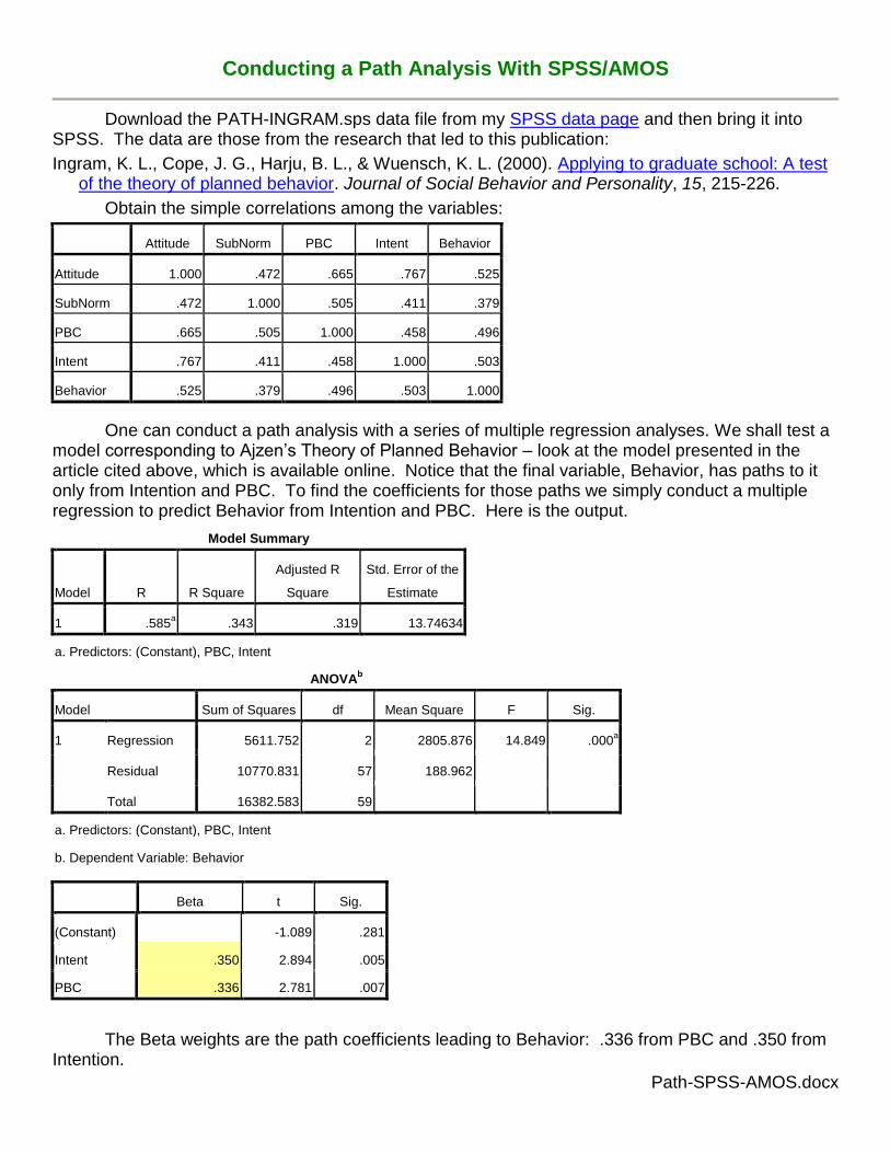
Obtain the simple correlations among the variables:
Attitude SubNorm PBC Intent Behavior
Attitude 1.000 .472 .665 .767 .525
SubNorm .472 1.000 .505 .411 .379
PBC .665 .505 1.000 .458 .496
Intent .767 .411 .458 1.000 .503
Behavior .525 .379 .496 .503 1.000
One can conduct a path analysis with a series of multiple regression analyses. We shall test a model corresponding to Ajzen’s Theory of Planned Behavior – look at the model presented in the article cited above, which is available online. Notice that the final variable, Behavior, has paths to it only from Intention and PBC. To find the coefficients for those paths we simply conduct a multiple regression to predict Behavior from Intention and PBC. Here is the output.
Model Summary
Model R R Square
Adjusted R
Square
Std. Error of the
Estimate
1 .585a .343 .319 13.74634
a. Predictors: (Constant), PBC, Intent
ANOVAb
Model Sum of Squares df Mean Square F Sig.
1 Regression 5611.752 2 2805.876 14.849 .000a
Residual 10770.831 57 188.962
Total 16382.583 59
a. Predictors: (Constant), PBC, Intent
b. Dependent Variable: Behavior
Beta t Sig.
(Constant) -1.089 .281
Intent .350 2.894 .005
PBC .336 2.781 .007
The Beta weights are the path coefficients leading to Behavior: .336 from PBC and .350 from Intention.

2
In the model, Intention has paths to it from Attitude, Subjective Norm, and Perceived Behavioral Control, so we predict Intention from Attitude, Subjective Norm, and Perceived Behavioral Control. Here is the output:
Model Summary
Model R R Square
Adjusted R
Square
Std. Error of the
Estimate
1 .774a .600 .578 2.48849
a. Predictors: (Constant), PBC, SubNorm, Attitude
ANOVAb
Model Sum of Squares df Mean Square F Sig.
1 Regression 519.799 3 173.266 27.980 .000a
Residual 346.784 56 6.193
Total 866.583 59
a. Predictors: (Constant), PBC, SubNorm, Attitude
b. Dependent Variable: Intent
Beta t Sig.
(Constant) 2.137 .037
Attitude .807 6.966 .000
SubNorm .095 .946 .348
PBC -.126 -1.069 .290
The path coefficients leading to Intention are: .807 from Attitude, .095 from Subjective Norms,
and .126 from Perceived Behavioral Control.
AMOS Now let us use AMOS. The data file is already open in SPSS. Click Analyze, IBM SPSS AMOS. In the AMOS window which will open click File, New:
3
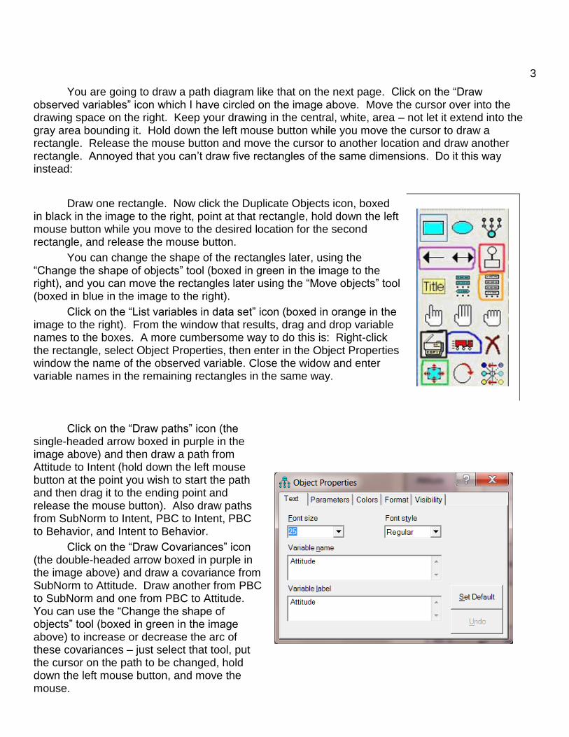
You are going to draw a path diagram like that on the next page. Click on the “Draw observed variables” icon which I have circled on the image above. Move the cursor over into the drawing space on the right. Keep your drawing in the central, white, area – not let it extend into the gray area bounding it. Hold down the left mouse button while you move the cursor to draw a rectangle. Release the mouse button and move the cursor to another location and draw another rectangle. Annoyed that you can’t draw five rectangles of the same dimensions. Do it this way instead:
Draw one rectangle. Now click the Duplicate Objects icon, boxed in black in the image to the right, point at that rectangle, hold down the left mouse button while you move to the desired location for the second rectangle, and release the mouse button.
You can change the shape of the rectangles later, using the “Change the shape of objects” tool (boxed in green in the image to the right), and you can move the rectangles later using the “Move objects” tool (boxed in blue in the image to the right).
Click on the “List variables in data set” icon (boxed in orange in the image to the right). From the window that results, drag and drop variable names to the boxes. A more cumbersome way to do this is: Right-click the rectangle, select Object Properties, then enter in the Object Properties window the name of the observed variable. Close the widow and enter variable names in the remaining rectangles in the same way.
Click on the “Draw paths” icon (the single-headed arrow boxed in purple in the image above) and then draw a path from Attitude to Intent (hold down the left mouse button at the point you wish to start the path and then drag it to the ending point and release the mouse button). Also draw paths from SubNorm to Intent, PBC to Intent, PBC to Behavior, and Intent to Behavior.
Click on the “Draw Covariances” icon (the double-headed arrow boxed in purple in the image above) and draw a covariance from SubNorm to Attitude. Draw another from PBC to SubNorm and one from PBC to Attitude. You can use the “Change the shape of objects” tool (boxed in green in the image above) to increase or decrease the arc of these covariances – just select that tool, put the cursor on the path to be changed, hold down the left mouse button, and move the mouse.

4
Click on the “Add a unique variable to an existing variable” icon (boxed in red in the image above) and then move the cursor over the Intent variable and click the left mouse button to add the error variable. Do the same to add an error variable to the Behavior variable. Right-click the error circle leading to Intent, select Object Properties, and name the variable “e1.” Name the other error circle “e2.”
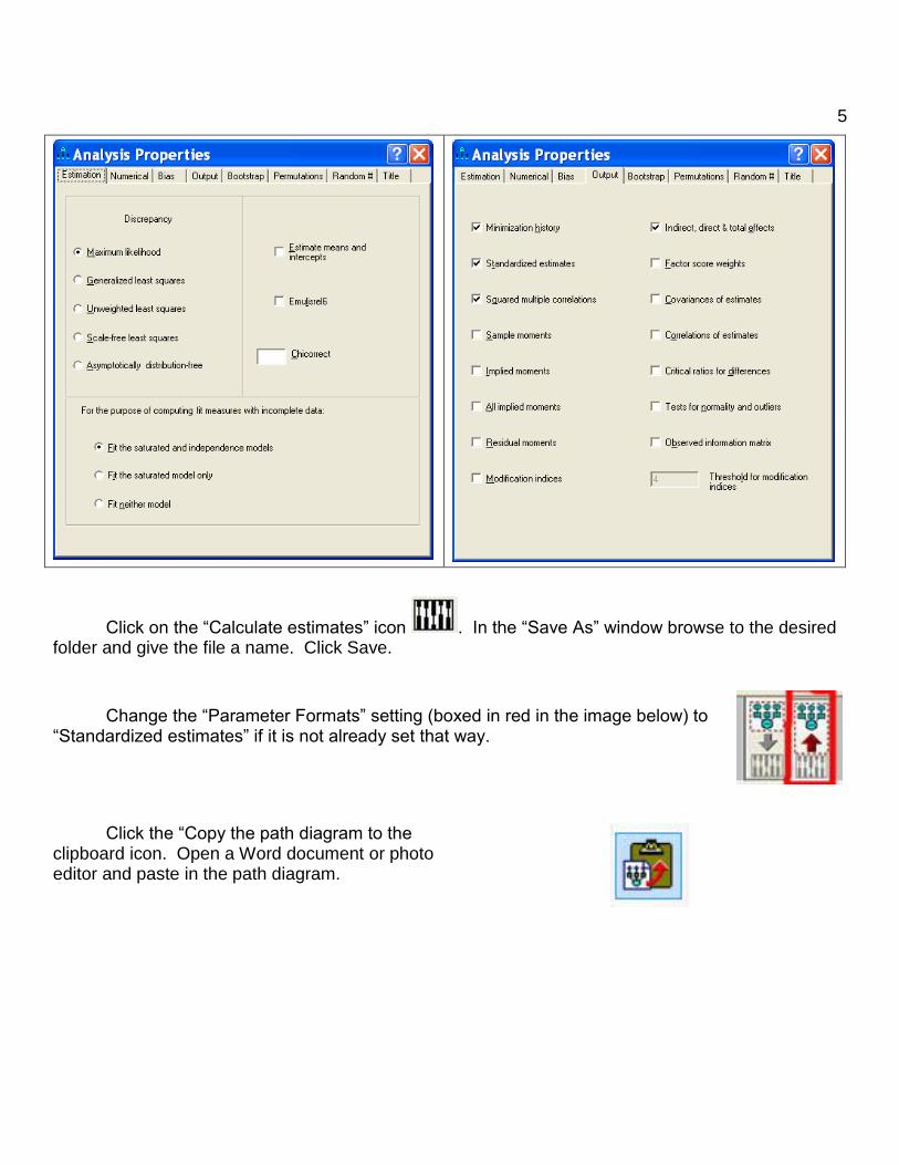
Click the “Analysis properties” icon -- to display the Analysis Properties window. Select the Output tab and ask for the output shown below.
5
Click on the “Calculate estimates” icon . In the “Save As” window browse to the desired folder and give the file a name. Click Save.
Change the “Parameter Formats” setting (boxed in red in the image below) to “Standardized estimates” if it is not already set that way.
Click the “Copy the path diagram to the clipboard icon. Open a Word document or photo editor and paste in the path diagram.
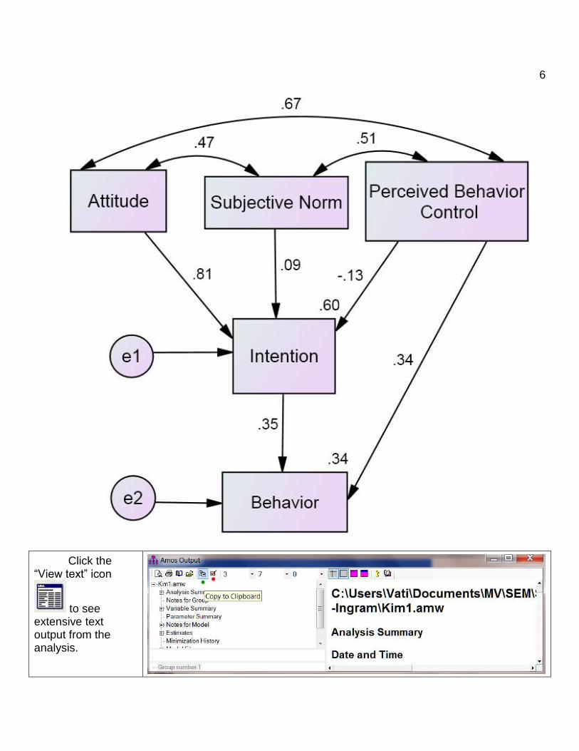
6
Click the “View text” icon
to see extensive text output from the analysis.
7
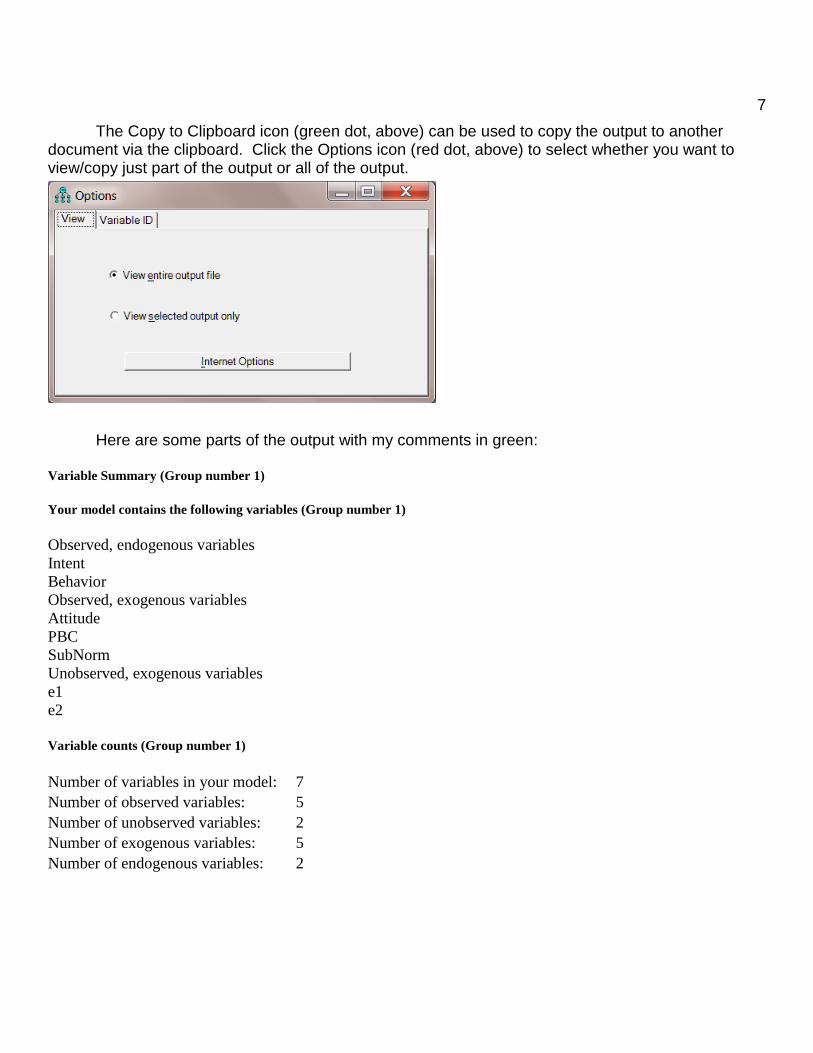
The Copy to Clipboard icon (green dot, above) can be used to copy the output to another document via the clipboard. Click the Options icon (red dot, above) to select whether you want to view/copy just part of the output or all of the output.
Here are some parts of the output with my comments in green:
Variable Summary (Group number 1)
Your model contains the following variables (Group number 1)
Observed, endogenous variables
Intent
Behavior
Observed, exogenous variables
Attitude
PBC
SubNorm
Unobserved, exogenous variables
e1
e2
Variable counts (Group number 1)
Number of variables in your model: 7
Number of observed variables: 5
Number of unobserved variables: 2
Number of exogenous variables: 5
Number of endogenous variables: 2

8
Parameter summary (Group number 1)
Weights Covariances Variances Means Intercepts Total
Fixed 2 0 0 0 0 2
Labeled 0 0 0 0 0 0
Unlabeled 5 3 5 0 0 13
Total 7 3 5 0 0 15
Models
Default model (Default model)
Notes for Model (Default model)
Computation of degrees of freedom (Default model)
Number of distinct sample moments: 15
Number of distinct parameters to be estimated: 13
Degrees of freedom (15 - 13): 2
Result (Default model)
Minimum was achieved
Chi-square = .847
Degrees of freedom = 2
Probability level = .655
This Chi-square tests the null hypothesis that the overidentified (reduced) model fits the data as well as does a just-identified (full, saturated) model. In a just-identified model there is a direct path (not through an intervening variable) from each variable to each other variable. When you delete one or more of the paths you obtain an overidentified model. The nonsignificant Chi-square here indicated that the fit between our overidentified model and the data is not significantly worse than the fit between the just-identified model and the data. You can see the just-identified model here. While one might argue that nonsignificance of this Chi-square indicates that the reduced model fits the data well, even a well-fitting reduced model will be significantly different from the full model if sample size is sufficiently large. A good fitting model is one that can reproduce the original variance-covariance matrix (or correlation matrix) from the path coefficients, in much the same way that a good factor analytic solution can reproduce the original correlation matrix with little error.
Maximum Likelihood Estimates
Do note that the parameters are estimated by maximum likelihood (ML) methods rather than by ordinary least squares (OLS) methods. OLS methods minimize the squared deviations between values of the criterion variable and those predicted by the model. ML (an iterative procedure) attempts to maximize the likelihood that obtained values of the criterion variable will be correctly predicted.

9
Standardized Regression Weights: (Group number 1 - Default model)
Estimate
Intent SubNorm .095
Intent PBC -.126
Intent Attitude .807
Behavior Intent .350
Behavior PBC .336
The path coefficients above match those we obtained earlier by multiple regression.
Correlations: (Group number 1 - Default model)
Estimate
Attitude <--> PBC .665
Attitude <--> SubNorm .472
PBC <--> SubNorm .505
Above are the simple correlations between exogenous variables.
Squared Multiple Correlations: (Group number 1 - Default model)
Estimate
Intent .600
Behavior .343
Above are the squared multiple correlation coefficients we saw in the two multiple regressions.
The total effect of one variable on another can be divided into direct effects (no intervening variables involved) and indirect effects (through one or more intervening variables). Consider the effect of PBC on Behavior. The direct effect is .336 (the path coefficient from PBC to Behavior). The indirect effect, through Intention is computed as the product of the path coefficient from PBC to Intention and the
path coefficient from Intention to Behavior, (.126)(.350) = .044. The total effect is the sum of direct
and indirect effects, .336 + (.126) = .292.
Standardized Total Effects (Group number 1 - Default model)
SubNorm PBC Attitude Intent
Intent .095 -.126 .807 .000
Behavior .033 .292 .282 .350
10
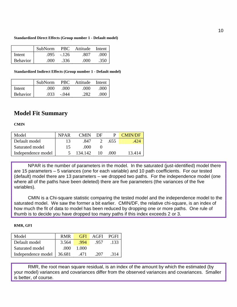
Standardized Direct Effects (Group number 1 - Default model)
SubNorm PBC Attitude Intent
Intent .095 -.126 .807 .000
Behavior .000 .336 .000 .350
Standardized Indirect Effects (Group number 1 - Default model)
SubNorm PBC Attitude Intent
Intent .000 .000 .000 .000
Behavior .033 -.044 .282 .000
Model Fit Summary
CMIN
Model NPAR CMIN DF P CMIN/DF
Default model 13 .847 2 .655 .424
Saturated model 15 .000 0
Independence model 5 134.142 10 .000 13.414
NPAR is the number of parameters in the model. In the saturated (just-identified) model there are 15 parameters – 5 variances (one for each variable) and 10 path coefficients. For our tested (default) model there are 13 parameters – we dropped two paths. For the independence model (one where all of the paths have been deleted) there are five parameters (the variances of the five variables).
CMIN is a Chi-square statistic comparing the tested model and the independence model to the saturated model. We saw the former a bit earlier. CMIN/DF, the relative chi-square, is an index of how much the fit of data to model has been reduced by dropping one or more paths. One rule of thumb is to decide you have dropped too many paths if this index exceeds 2 or 3.
RMR, GFI
Model RMR GFI AGFI PGFI
Default model 3.564 .994 .957 .133
Saturated model .000 1.000
Independence model 36.681 .471 .207 .314
RMR, the root mean square residual, is an index of the amount by which the estimated (by your model) variances and covariances differ from the observed variances and covariances. Smaller is better, of course.

11
GFI, the goodness of fit index, tells you what proportion of the variance in the sample variance-covariance matrix is accounted for by the model. This should exceed .9 for a good model. For the saturated model it will be a perfect 1. AGFI (adjusted GFI) is an alternate GFI index in which the value of the index is adjusted for the number of parameters in the model. The fewer the number of parameters in the model relative to the number of data points (variances and covariances in the sample variance-covariance matrix), the closer the AGFI will be to the GFI. The PGFI (P is for parsimony), the index is adjusted to reward simple models and penalize models in which few paths have been deleted. Note that for our data the PGFI is larger for the independence model than for our tested model.
Baseline Comparisons
Model NFI
Delta1
RFI
rho1
IFI
Delta2
TLI
rho2 CFI
Default model .994 .968 1.009 1.046 1.000
Saturated model 1.000 1.000 1.000
Independence model .000 .000 .000 .000 .000
These goodness of fit indices compare your model to the independence model rather than to the saturated model. The Normed Fit Index (NFI) is simply the difference between the two models’ chi-squares divided by the chi-square for the independence model. For our data, that is (134.142)-.847)/134.142 = .994. Values of .9 or higher (some say .95 or higher) indicate good fit. The Comparative Fit Index (CFI) uses a similar approach (with a noncentral chi-square) and is said to be a good index for use even with small samples. It ranges from 0 to 1, like the NFI, and .95 (or .9 or higher) indicates good fit.
Parsimony-Adjusted Measures
Model PRATIO PNFI PCFI
Default model .200 .199 .200
Saturated model .000 .000 .000
Independence model 1.000 .000 .000
PRATIO is the ratio of how many paths you dropped to how many you could have dropped (all of them). The Parsimony Normed Fit Index (PNFI), is the product of NFI and PRATIO, and PCFI is the product of the CFI and PRATIO. The PNFI and PCFI are intended to reward those whose models are parsimonious (contain few paths).
12
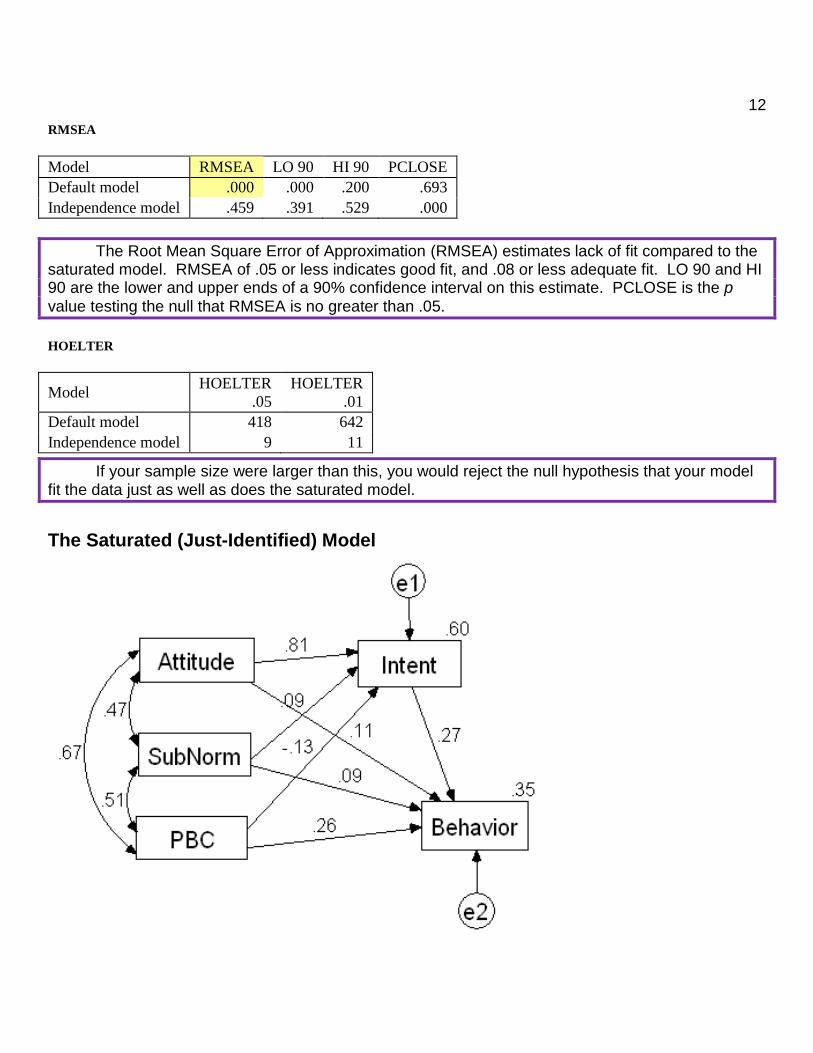
RMSEA
Model RMSEA LO 90 HI 90 PCLOSE
Default model .000 .000 .200 .693
Independence model .459 .391 .529 .000
The Root Mean Square Error of Approximation (RMSEA) estimates lack of fit compared to the saturated model. RMSEA of .05 or less indicates good fit, and .08 or less adequate fit. LO 90 and HI 90 are the lower and upper ends of a 90% confidence interval on this estimate. PCLOSE is the p
value testing the null that RMSEA is no greater than .05.
HOELTER
Model HOELTER
.05
HOELTER
.01
Default model 418 642
Independence model 9 11
If your sample size were larger than this, you would reject the null hypothesis that your model fit the data just as well as does the saturated model.
The Saturated (Just-Identified) Model

13
Matrix Input
AMOS will accept as input a correlation matrix (accompanied by standard deviations and sample sizes) or a variance/covariance matrix. The SPSS syntax below would input such a matrix:
MATRIX DATA VARIABLES=ROWTYPE_ Attitude SubNorm PBC Intent Behavior. BEGIN DATA N 60 60 60 60 60 SD 6.96 12.32 7.62 3.83 16.66 CORR 1 CORR .472 1 CORR .665 .505 1 CORR .767 .411 .458 1 CORR .525 .379 .496 .503 1 END DATA.
After running the syntax you would just click Analyze, AMOS, and proceed as before. If you had the correlations but not the standard deviations, you could just specify a value of 1 for each standard deviation. You would not be able to get the unstandardized coefficients, but they are generally not of interest anyhow.
AMOS Files
Amos creates several files during the course of conducting a path analysis. Here is what I have learned about them, mostly by trial and error.
.amw = a path diagram, with coefficients etc.
.amp = table output – all the statistical output details. Open it with the AMOS file manager.
.AmosOutput – looks the same as .amp, but takes up more space on drive.
.AmosTN = thumbnail image of path diagram
*.bk# -- probably a backup file
Bringing Up an Old Path Diagram
Open up the data file in SPSS and then Analyze, AMOS. The path diagram will appear. Make any modifications you want and then submit the analysis. If you have access to my BlackBoard files, do this:
1. Open Path-Ingram.sav in SPSS. 2. Analyze, AMOS 3. File, Open, Path-Ingram.amw 4. Calculate Estimates
AMOS Bugs
The last time I taught this lesson (October, 2014), with the students drawing the path diagram etc., when we asked for the analysis about half of us were told that one or more variables were not named. Checking the properties of each element of the diagram, we confirmed that all variables were named. I have encountered this error much too often, and my experience has been that the only way to resolve it is to start all over again. Very annoying !

14
The last time I renewed the license code for AMOS, every time I tried to run AMOS it told me the license had expired, despite the license authorization wizard having told me that the license had been successfully renewed and would not expire until the following year. I had to completely uninstall and then reinstall AMOS to get it to work.
Notes
To bring a path diagram into Word, just Edit, Copy to Clipboard, and then paste it into Word.
If you pull up an .amw path diagram but have not specified an input data file, you cannot alter
the diagram and re-analyze the data. The .amw file includes the coefficients etc., but not the input data.
If you input an altered data file and then call up the original .amw, you can Calculate Estimates again and get a new set of coefficients etc. WARNING – when you exit you will find that
the old .amp and .AmosOutput have been updated with the results of the analysis on the modified
data. The original .amw file remains unaltered.
Links
Introduction to Path Analysis – maybe more than you want to know.
Wuensch’s Stats Lessons Page
Karl L. Wuensch Dept. of Psychology East Carolina University Greenville, NC 27858-4353
October, 2013


