
THE USE OF PEAKVUE FOR FAULT DETECTION AND SEVERITY ASSESSMENT: DEMONSTRATED THROUGH REPRESENTATIVE CASE STUDIES
James C. Robinson
Emerson Process Management
Abstract: The primary focus in this paper is to demonstrate through several case studies the usefulness of incorporating stress wave analysis into the overall machine condition monitoring program for fault detection, identification, and severity assessment. The analysis methodology employed is the peak value (PeakVue) analysis methodology implemented in the CSI hardware. Emphasis is placed on measurement setup, sensor selection and placement, importance of trending, and severity assessment. Common defects, which generate stress waves, are pitting in antifriction bearings causing the rollers to impact, fatigue cracking in bearing raceways or gear teeth (generally at the root), scuffing or scoring on gear teeth or antifriction bearing components and others. Each event generally introduces a short term (microseconds to milliseconds) burst of stress wave activity which propagates away from the initiation site at the speed of sound in the medium. The dominate frequency within each burst of activity is inversely related to the duration of the event (short term events, microseconds, excite higher frequencies than long term events, milliseconds). The duration of events is dependent on the initiating source, mass, and speed. The general nature of stress wave activity versus initiating source is briefly discussed in this paper. Case studies are presented which encompass a large variation in stress wave activity. The emphasis will be placed on fault detection, fault classification, severity assessment, measurement setup, sensor selection, and sensor location. The case studies will demonstrate that stress wave analysis provide (1) meaningful backup to normal analysis in some situations and (2) the only means for fault detection, classification, and severity assessment for other situations.
1.0 Introduction
Many faults within rotating machinery will introduce both vibration and stress wave* activity. Both provide 1) a means of detecting the presence of a fault and 2) means of classifying the severity of the fault. In this paper, the emphasis is place on stress wave activity:
1. Condensed understanding of the basic properties governing stress wave initiation, propagation,
and detection. 2. Demonstration (through case studies) of stress wave analysis for fault detection and severity
assessment on a variety of rotating machinery representative of a broad industrial market. In the next section, stress wave generation, propagation, detection, and the analysis methodology is presented. The third section will present recommended measurement setup for 1) data capture and analysis and 2) parameters for trending with alert/fault levels. The fourth section will consist of several case studies selected to illustrate both benefits and expected behavior of stress wave analysis applied to condition monitoring programs for industrial rotating machinery. The last section consists of conclusions and recommendation for stress wave analysis.
2.0 Stress Waves
2.1 Introduction In this section, the intent is to present a basic discussion on the generation of stress waves commonly induced from faults within rotating machinery. The propagation for these stress waves from the initiation site to the detection site, role of the sensor in the detection of stress waves from various sources, and the analysis methodology employed by CSI.
*Stress waves introduced by many faults in rotating machinery are short term transient events which introduce ripple on the machinery surface as they propagate away from the initiation site.
2.2 Quantitative Framework for Understanding Stress Waves
Stress Waves can be generated in any elastic medium. The primary interest focused on within this study is in rotating machinery. Stress waves accompany the sudden displacement of small amounts of material in a very short time period.1 In rotating machinery, this occurs when impacting, fatigue cracking, scuffing, abrasive wear, etc. occurs. The most frequent occurrences of stress wave generation in rotating machinery are observed in fault initiation and progression in both rolling element bearings and in gear teeth. Once the stress waves are generated, they propagate away from the initiation site at the speed of sound in the particular medium (metal) being evaluated. A quantitative framework for the generation and detection of stress waves can be developed using the Hertz theory for metal-to-metal impacting2 and wave theory3 for propagation of stress waves in metal. We consider the brief discussion presented below on the theory of generation and propagation of stress waves to provide insight to:
1. Selection of sensor for the detection of stress waves,
2. Identification and localization of the fault introducing the stress waves, and
3. Severity assessment of the fault.
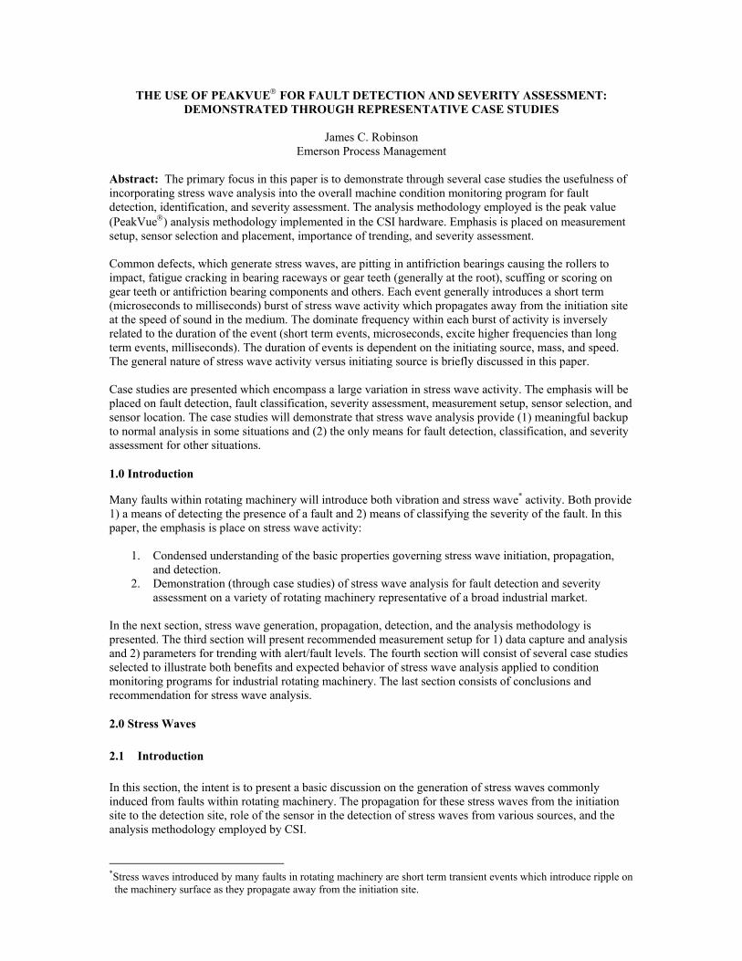
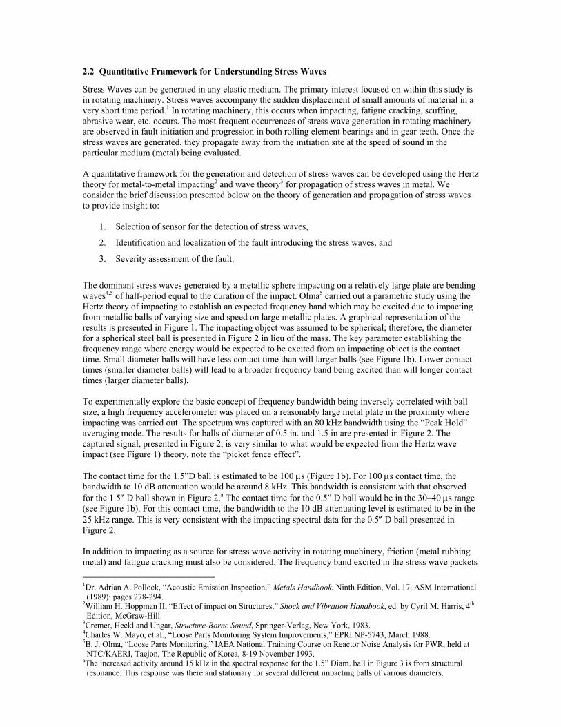
The dominant stress waves generated by a metallic sphere impacting on a relatively large plate are bending waves4,5 of half-period equal to the duration of the impact. Olma5 carried out a parametric study using the Hertz theory of impacting to establish an expected frequency band which may be excited due to impacting from metallic balls of varying size and speed on large metallic plates. A graphical representation of the results is presented in Figure 1. The impacting object was assumed to be spherical; therefore, the diameter for a spherical steel ball is presented in Figure 2 in lieu of the mass. The key parameter establishing the frequency range where energy would be expected to be excited from an impacting object is the contact time. Small diameter balls will have less contact time than will larger balls (see Figure 1b). Lower contact times (smaller diameter balls) will lead to a broader frequency band being excited than will longer contact times (larger diameter balls). To experimentally explore the basic concept of frequency bandwidth being inversely correlated with ball size, a high frequency accelerometer was placed on a reasonably large metal plate in the proximity where impacting was carried out. The spectrum was captured with an 80 kHz bandwidth using the “Peak Hold” averaging mode. The results for balls of diameter of 0.5 in. and 1.5 in are presented in Figure 2. The captured signal, presented in Figure 2, is very similar to what would be expected from the Hertz wave impact (see Figure 1) theory, note the “picket fence effect”. The contact time for the 1.5”D ball is estimated to be 100 µs (Figure 1b). For 100 µs contact time, the bandwidth to 10 dB attenuation would be around 8 kHz. This bandwidth is consistent with that observed for the 1.5″ D ball shown in Figure 2.a The contact time for the 0.5” D ball would be in the 30–40 µs range (see Figure 1b). For this contact time, the bandwidth to the 10 dB attenuating level is estimated to be in the 25 kHz range. This is very consistent with the impacting spectral data for the 0.5″ D ball presented in Figure 2. In addition to impacting as a source for stress wave activity in rotating machinery, friction (metal rubbing metal) and fatigue cracking must also be considered. The frequency band excited in the stress wave packets 1Dr. Adrian A. Pollock, “Acoustic Emission Inspection,” Metals Handbook, Ninth Edition, Vol. 17, ASM International (1989): pages 278-294.
2William H. Hoppman II, “Effect of impact on Structures.” Shock and Vibration Handbook, ed. by Cyril M. Harris, 4th Edition, McGraw-Hill.
3Cremer, Heckl and Ungar, Structure-Borne Sound, Springer-Verlag, New York, 1983. 4Charles W. Mayo, et al., “Loose Parts Monitoring System Improvements,” EPRI NP-5743, March 1988. 5B. J. Olma, “Loose Parts Monitoring,” IAEA National Training Course on Reactor Noise Analysis for PWR, held at NTC/KAERI, Taejon, The Republic of Korea, 8-19 November 1993.
aThe increased activity around 15 kHz in the spectral response for the 1.5” Diam. ball in Figure 3 is from structural resonance. This response was there and stationary for several different impacting balls of various diameters.
0.5” Dia.Ball
1.5” Dia.Ball
Figure 1. Hertz theory prediction for metal balls for varying size and speed impacting on large metal
plates.
Figure 2. Spectral data captured for a 0.5” Dia. and a 1.5” Dia. metal ball. Impacting on a large metal plate.
will still generally follow the Hertz theory if the equivalent contact time can be approximated (that time where material movement is present on a microscopic scale). In general, the equivalent contact time for friction will be less than that for impacting therefore the dominant frequency in a friction induced event will be greater than that in impacting events. This will be demonstrated in some case studies presented later in this paper.
2.3 Propagation of Stress Waves to Detection Site
Bending (versus longitudinal) waves are the most dominant stress waves generated in events experienced on rotating machinery.2,4,5 The velocity at which bending waves propagate away from the initiation site is proportional to the square root of frequency. Thus there will be dispersion within the stress wave packet when viewed (detected) at locations removed from the initiation site (the amplitude of the event will decrease and the duration of the event will increase as the observation point is further removed from the initiation site). In addition to the diffusion of the stress wave packet, the attenuation of the stress waves are also frequency dependent 3,6 with the higher frequency components attenuating faster than the lower frequency components as the observation (measurement) point is removed from the point of origin. This is especially true when stress wave packets must cross physical interfaces such as from shaft (or inner race of a bearing) to get to the observation point on the outer structure of the machine.
2.4 Selecting the Sensor and Location
Due to the dispersion and attenuation of the stress wave packet, it is desirable to locate the sensor as near to the initiation site as possible. This generally will be near or on the bearing housing (preferably in the load zone). Stress waves will propagate in all directions. Hence the selection of axial, vertical, or radial is less (relative to normal vibration monitoring) of an issue than is mounting the sensor in or near the load zone with the caution that we are monitoring “waves” and hence, must always be cautious of encountering nodal points which can occur due to multi-path transmission and in the vicinity of sharp corners, etc. The bending stress waves introduce a ripple. Hence any sensor which is sensitive to absolute motion occurring at a high rate would suffice, providing it has sufficient frequency range and amplitude resolution capabilities. Therefore, this sensor could be an accelerometer with sufficient bandwidth, an ultrasonic sensor, a strain gauge, piezoelectric film, et al. The primary motivation behind stress wave monitoring is to acquire information for machine health monitoring which is the motivation behind vibration monitoring in a predictive maintenance program. By far, the most common sensor employed in vibration monitoring is the accelerometer; therefore the sensor of choice for stress wave monitoring is the accelerometer. The requirements for this sensor will be sufficient analysis bandwidth (frequency range), amplitude resolution and appropriate sensitivity. The bandwidth of an accelerometer is dependent on (1) its design and (2) the manner in which the accelerometer is attached to the surface. The general effect, which different mounting schemes have on the sensor bandwidth, are presented in Figure 3 (sensor becomes entire system attached to the surface).
2.4 Analysis of Stress Waves
The analog output of an accelerometer located on a machine will include classic vibration and stress wave induced activity over the entire response bandwidth of the sensor system. The stress wave-induced component of the accelerometer signal is generally separated from the normal vibration by routing the signal through a high order high-pass filter. The methodology developed by CSI (PeakVue) for processing the signal (made up of frequencies exceeding the high pass filter setting) are tabulated below:
6Richard H. Lyon , Machinery Noise and Diagnostics, Butterworth, 1987.
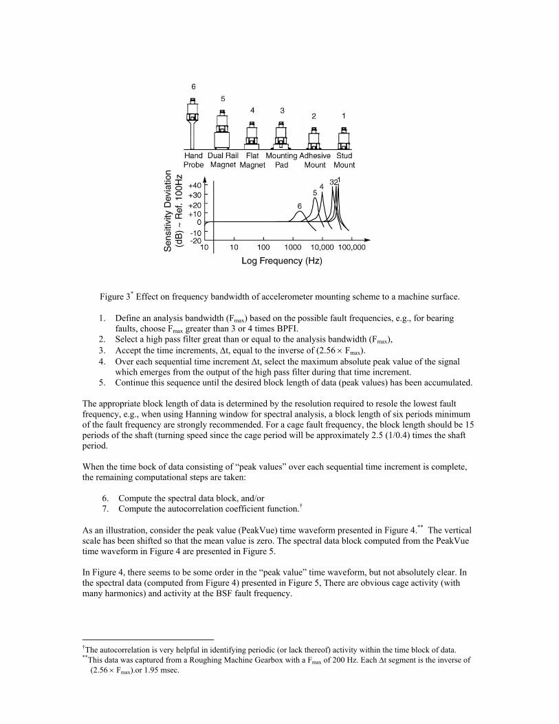
Figure 3* Effect on frequency bandwidth of accelerometer mounting scheme to a machine surface.
1. Define an analysis bandwidth (Fmax) based on the possible fault frequencies, e.g., for bearing faults, choose Fmax greater than 3 or 4 times BPFI.
2. Select a high pass filter great than or equal to the analysis bandwidth (Fmax), 3. Accept the time increments, ∆t, equal to the inverse of (2.56 × Fmax). 4. Over each sequential time increment ∆t, select the maximum absolute peak value of the signal
which emerges from the output of the high pass filter during that time increment. 5. Continue this sequence until the desired block length of data (peak values) has been accumulated.
The appropriate block length of data is determined by the resolution required to resole the lowest fault frequency, e.g., when using Hanning window for spectral analysis, a block length of six periods minimum of the fault frequency are strongly recommended. For a cage fault frequency, the block length should be 15 periods of the shaft (turning speed since the cage period will be approximately 2.5 (1/0.4) times the shaft period. When the time bock of data consisting of “peak values” over each sequential time increment is complete, the remaining computational steps are taken:
6. Compute the spectral data block, and/or 7. Compute the autocorrelation coefficient function.†
As an illustration, consider the peak value (PeakVue) time waveform presented in Figure 4.** The vertical scale has been shifted so that the mean value is zero. The spectral data block computed from the PeakVue time waveform in Figure 4 are presented in Figure 5. In Figure 4, there seems to be some order in the “peak value” time waveform, but not absolutely clear. In the spectral data (computed from Figure 4) presented in Figure 5, There are obvious cage activity (with many harmonics) and activity at the BSF fault frequency.
†The autocorrelation is very helpful in identifying periodic (or lack thereof) activity within the time block of data. **This data was captured from a Roughing Machine Gearbox with a Fmax of 200 Hz. Each ∆t segment is the inverse of
(2.56 × Fmax).or 1.95 msec.
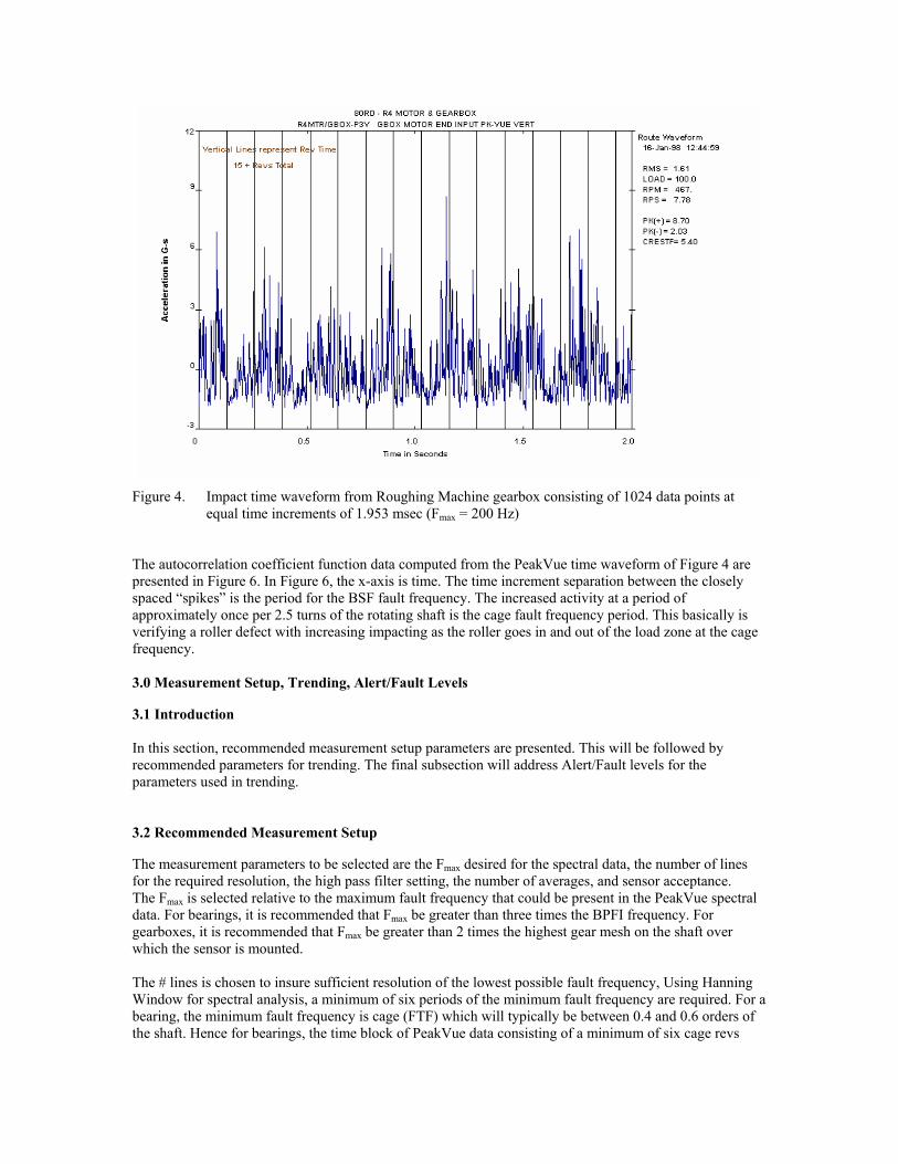
Figure 4. Impact time waveform from Roughing Machine gearbox consisting of 1024 data points at
equal time increments of 1.953 msec (Fmax = 200 Hz) The autocorrelation coefficient function data computed from the PeakVue time waveform of Figure 4 are presented in Figure 6. In Figure 6, the x-axis is time. The time increment separation between the closely spaced “spikes” is the period for the BSF fault frequency. The increased activity at a period of approximately once per 2.5 turns of the rotating shaft is the cage fault frequency period. This basically is verifying a roller defect with increasing impacting as the roller goes in and out of the load zone at the cage frequency. 3.0 Measurement Setup, Trending, Alert/Fault Levels
3.1 Introduction In this section, recommended measurement setup parameters are presented. This will be followed by recommended parameters for trending. The final subsection will address Alert/Fault levels for the parameters used in trending. 3.2 Recommended Measurement Setup
The measurement parameters to be selected are the Fmax desired for the spectral data, the number of lines for the required resolution, the high pass filter setting, the number of averages, and sensor acceptance. The Fmax is selected relative to the maximum fault frequency that could be present in the PeakVue spectral data. For bearings, it is recommended that Fmax be greater than three times the BPFI frequency. For gearboxes, it is recommended that Fmax be greater than 2 times the highest gear mesh on the shaft over which the sensor is mounted. The # lines is chosen to insure sufficient resolution of the lowest possible fault frequency, Using Hanning Window for spectral analysis, a minimum of six periods of the minimum fault frequency are required. For a bearing, the minimum fault frequency is cage (FTF) which will typically be between 0.4 and 0.6 orders of the shaft. Hence for bearings, the time block of PeakVue data consisting of a minimum of six cage revs
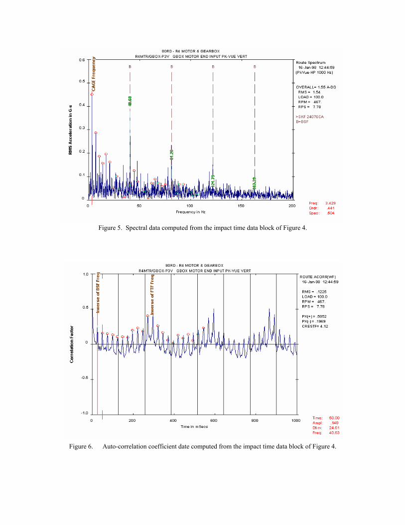
Figure 5. Spectral data computed from the impact time data block of Figure 4.
Figure 6. Auto-correlation coefficient date computed from the impact time data block of Figure 4.
That is approximately 15 shaft periods.* The upper limit on the # of lines is controlled by the time data block which can be stored by the data collector being used. The high pass filter, Fhp, is selected to be greater than or equal to Fmax. On a gear box,** it is recommended the same Fhp filter setting be employed for all measurement points on that gear box and hence equal or greater than the maximum Fmax on the gear box. The Fmax will vary (lower when measurement point over the slower shafts relative to the high speed shaft). In PeakVue measurements, the PeakVue time waveform has equal or greater importance than the spectral data. When averaging is employed in normal vibration analysis, the objective is to improve “signal-to-noise” in the spectral data with little attention paid to the time waveform. In PeakVue, it is highly recommended that both the spectral and PeakVue time wave data be captures and returned to the database. The recommendation is to use one block (no special waveform) analysis in sensor units. The signal-to-noise ratio is improved† by increasing number of lines versus multiple block averaging. Once the Fhp is selected, attention is then diverted to the sensor selection and mounting scheme. The general effect of sensor mounting is presented in Figure 3. This data was experimentally collected under idea conditions. The rail magnet in Figure 3 was measured on a flat smooth surface with lubricant on all interfaces. In the field using this mounting scheme on a clean rounded surface, the bandwidth will be reduced by about a factor of 2 or so. Thus if a Fhp greater than 2 kHz is required (5 kHz is the next choice in CSI hardware), very little stress wave activity will make it to the sensor. For rolling elements greater than ~0.75″ in diameter and Fhp equal to or less than 2 kHz, the stress wave activity will be detected by a sensor on rail-magnets assuming the rounded surface is clean and reasonably smooth. The success of detecting stress wave activity from fatiguing and friction are significantly reduced for the rail magnet mounting on curved smooth dry surfaces since the energy in stress pockets from fatigue and friction is at higher frequencies than impacting for rollers exceeding the 0.5″D, range. For rolling elements less than ≅ 0.5″ D, the choice of a rail magnet mounted sensors is not a good choice since the dominant frequency within the stress wave packets (including impacting) will be in the 5 + kHz range. 3.3 Trending of PeakVue Data The primary PeakVue parameter which should be used for trending PeakVue measurements is the parameter referred to as “Pk-Pk Waveform” that is available in the PdM software. Extensive field experience within PdM programs has shown the trending of PeakVue “Pk-Pk Waveform” has proven to be a reliable indicator for detection of faults caused by impact or impulse events (bearing, gear, lubrication, cavitation and related faults). The "Pk-Pk Waveform" parameter is not dependent on the analysis bandwidth or duty cycle of the events (note that the term “duty cycle” refers to the number of events per cycle or revolution; e.g., an inner race fault occurs more frequently than does a roller fault). This lack of dependence on analysis bandwidth or duty cycle permits generic alarm levels to be established. A second parameter that has proven to be very beneficial for trending is the digital overall level computed from the spectral data. It will be dependent on the duty cycle (fault type) and hence must be based on the “baseline” results. Other parameters could be useful but in general, not proven to be worth the effort required.
*A convenient formula for determining the number of periods in a time block of data was provided by Mr. Clyde
Bridges of Mitsubishi Polyester Film, LLC in Greer, SC. # of Revolutions = )ordersin ( F
lines of No
max
.
**Stress waves will propagate from the initiation site throughout the housing encasing the gearbox. †For signals containing periodic plus noise, the noise component is proportional to the ∆f of window. Hence double the number of lines decrease the noise by ½. Averaging requires 4 blocks for the same noise reduction.
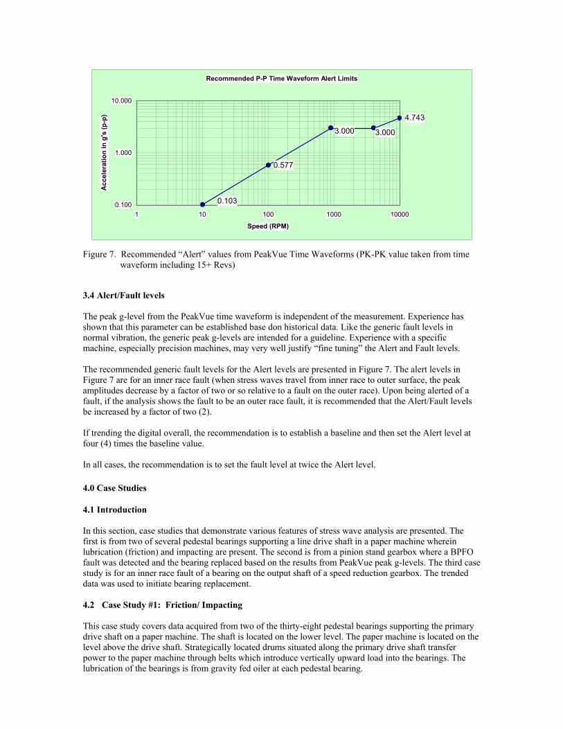
Recommended P-P Time Waveform Alert Limits
0.577
4.743
3.000 3.000
0.1030.100
1.000
10.000
1 10 100 1000 10000
Speed (RPM)
Acc
eler
atio
n in
g's
(p-p
)
Figure 7. Recommended “Alert” values from PeakVue Time Waveforms (PK-PK value taken from time
waveform including 15+ Revs)
3.4 Alert/Fault levels The peak g-level from the PeakVue time waveform is independent of the measurement. Experience has shown that this parameter can be established base don historical data. Like the generic fault levels in normal vibration, the generic peak g-levels are intended for a guideline. Experience with a specific machine, especially precision machines, may very well justify “fine tuning” the Alert and Fault levels. The recommended generic fault levels for the Alert levels are presented in Figure 7. The alert levels in Figure 7 are for an inner race fault (when stress waves travel from inner race to outer surface, the peak amplitudes decrease by a factor of two or so relative to a fault on the outer race). Upon being alerted of a fault, if the analysis shows the fault to be an outer race fault, it is recommended that the Alert/Fault levels be increased by a factor of two (2). If trending the digital overall, the recommendation is to establish a baseline and then set the Alert level at four (4) times the baseline value. In all cases, the recommendation is to set the fault level at twice the Alert level. 4.0 Case Studies
4.1 Introduction In this section, case studies that demonstrate various features of stress wave analysis are presented. The first is from two of several pedestal bearings supporting a line drive shaft in a paper machine wherein lubrication (friction) and impacting are present. The second is from a pinion stand gearbox where a BPFO fault was detected and the bearing replaced based on the results from PeakVue peak g-levels. The third case study is for an inner race fault of a bearing on the output shaft of a speed reduction gearbox. The trended data was used to initiate bearing replacement. 4.2 Case Study #1: Friction/ Impacting This case study covers data acquired from two of the thirty-eight pedestal bearings supporting the primary drive shaft on a paper machine. The shaft is located on the lower level. The paper machine is located on the level above the drive shaft. Strategically located drums situated along the primary drive shaft transfer power to the paper machine through belts which introduce vertically upward load into the bearings. The lubrication of the bearings is from gravity fed oiler at each pedestal bearing.
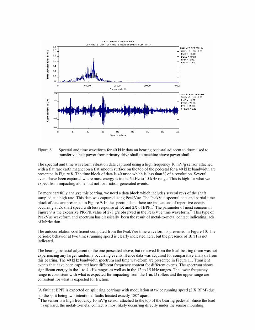
Figure 8. Spectral and time waveform for 40 kHz data on bearing pedestal adjacent to drum used to transfer via belt power from primary drive shaft to machine above power shaft.
The spectral and time waveform vibration data captured using a high frequency 10 mV/g sensor attached with a flat rare earth magnet on a flat smooth surface on the top of the pedestal for a 40 kHz bandwidth are presented in Figure 8. The time block of data is 40 msec which is less than ½ of a revolution. Several events have been captured where most energy is in the 6 kHz to 15 kHz range. This is high for what we expect from impacting alone, but not for friction-generated events. To more carefully analyze this bearing, we need a data block which includes several revs of the shaft sampled at a high rate. This data was captured using PeakVue. The PeakVue spectral data and partial time block of data are presented in Figure 9. In the spectral data, there are indications of repetitive events occurring at 2x shaft speed with less response at 1X and 2X of BPFI.* The parameter of most concern in Figure 9 is the excessive PK-PK value of 273 g’s observed in the PeakVue time waveform.** This type of PeakVue waveform and spectrum has classically been the result of metal-to-metal contact indicating lack of lubrication. The autocorrelation coefficient computed from the PeakVue time waveform is presented in Figure 10. The periodic behavior at two times running speed is clearly indicated here, but the presence of BPFI is not indicated. The bearing pedestal adjacent to the one presented above, but removed from the load-bearing drum was not experiencing any large, randomly occurring events. Hence data was acquired for comparative analysis from this bearing. The 40 kHz bandwidth spectrum and time waveform are presented in Figure 11. Transient events that have been captured have different frequency content for different events. The spectrum shows significant energy in the 1 to 4 kHz ranges as well as in the 12 to 15 kHz ranges. The lower frequency range is consistent with what is expected for impacting from the 1 in. D rollers and the upper range are consistent for what is expected for friction. *A fault at BPFI is expected on split ring bearings with modulation at twice running speed (2 X RPM) due to the split being two intentional faults located exactly 180° apart.
**The sensor is a high frequency 10 mV/g sensor attached to the top of the bearing pedestal. Since the load is upward, the metal-to-metal contact is most likely occurring directly under the sensor mounting.
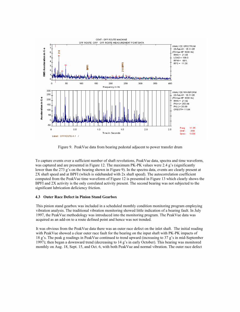
Figure 9. PeakVue data from bearing pedestal adjacent to power transfer drum To capture events over a sufficient number of shaft revolutions, PeakVue data, spectra and time waveform, was captured and are presented in Figure 12. The maximum PK-PK values were 2.4 g’s (significantly lower than the 273 g’s on the bearing shown in Figure 9). In the spectra data, events are clearly present at 2X shaft speed and at BPFI (which is sidebanded with 2x shaft speed). The autocorrelation coefficient computed from the PeakVue time waveform of Figure 12 is presented in Figure 13 which clearly shows the BPFI and 2X activity is the only correlated activity present. The second bearing was not subjected to the significant lubrication deficiency friction. 4.3 Outer Race Defect in Pinion Stand Gearbox
This pinion stand gearbox was included in a scheduled monthly condition monitoring program employing vibration analysis. The traditional vibration monitoring showed little indication of a bearing fault. In July 1997, the PeakVue methodology was introduced into the monitoring program. The PeakVue data was acquired as an add-on to a route defined point and hence was not trended. It was obvious from the PeakVue data there was an outer race defect on the inlet shaft. The initial reading with PeakVue showed a clear outer race fault for the bearing on the input shaft with PK-PK impacts of 18 g’s. The peak g readings in PeakVue continued to trend upward (increasing to 37 g’s in mid-September 1997); then began a downward trend (decreasing to 14 g’s in early October). This bearing was monitored monthly on Aug. 18, Sept. 15, and Oct. 6, with both PeakVue and normal vibration. The outer race defect
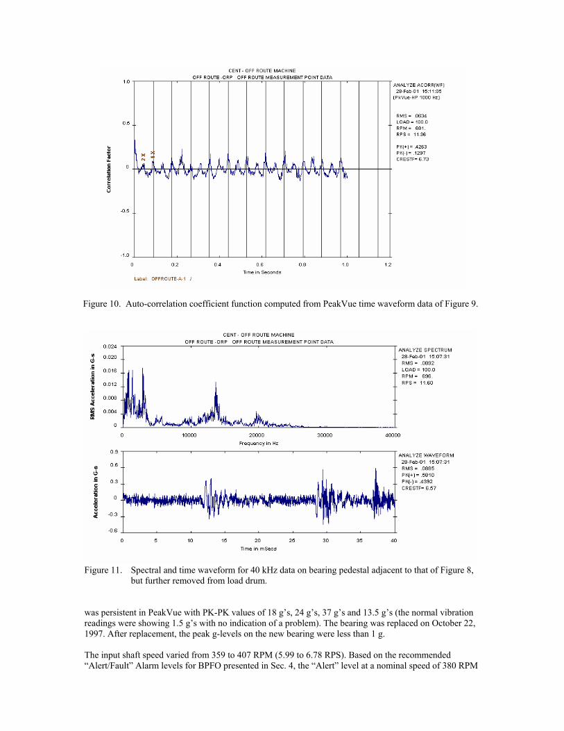
Figure 10. Auto-correlation coefficient function computed from PeakVue time waveform data of Figure 9.
Figure 11. Spectral and time waveform for 40 kHz data on bearing pedestal adjacent to that of Figure 8,
but further removed from load drum. was persistent in PeakVue with PK-PK values of 18 g’s, 24 g’s, 37 g’s and 13.5 g’s (the normal vibration readings were showing 1.5 g’s with no indication of a problem). The bearing was replaced on October 22, 1997. After replacement, the peak g-levels on the new bearing were less than 1 g. The input shaft speed varied from 359 to 407 RPM (5.99 to 6.78 RPS). Based on the recommended “Alert/Fault” Alarm levels for BPFO presented in Sec. 4, the “Alert” level at a nominal speed of 380 RPM

Figure 12. PeakVue Data bearing on Pedestal of Figure 11 (like that taken in Figure 9 on the bearing pedestal adjacent to power transfer drum).
Figure 13. Auto-correlation function coefficient function computed from PeakVue time waveform data for Figure 11.
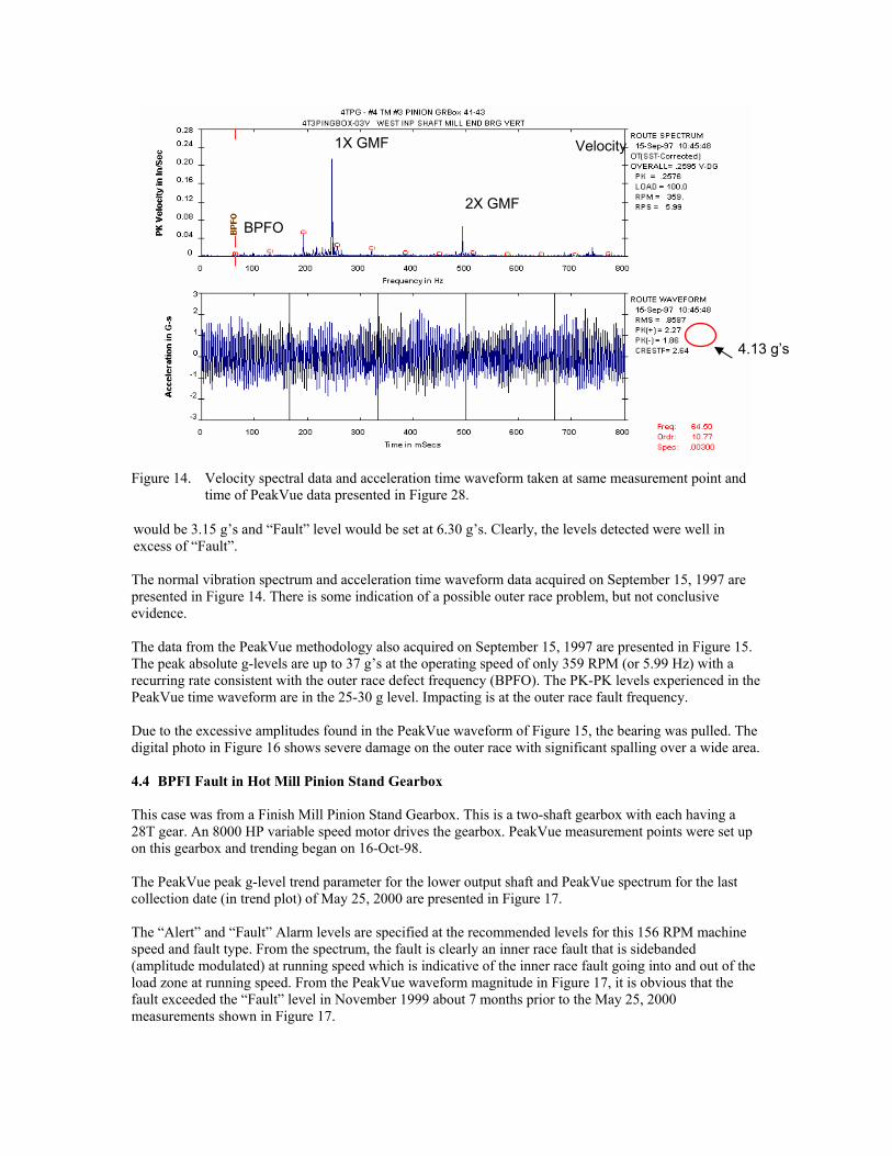
Figure 14. Velocity spectral data and acceleration time waveform taken at same measurement point and
time of PeakVue data presented in Figure 28.
would be 3.15 g’s and “Fault” level would be set at 6.30 g’s. Clearly, the levels detected were well in excess of “Fault”. The normal vibration spectrum and acceleration time waveform data acquired on September 15, 1997 are presented in Figure 14. There is some indication of a possible outer race problem, but not conclusive evidence. The data from the PeakVue methodology also acquired on September 15, 1997 are presented in Figure 15. The peak absolute g-levels are up to 37 g’s at the operating speed of only 359 RPM (or 5.99 Hz) with a recurring rate consistent with the outer race defect frequency (BPFO). The PK-PK levels experienced in the PeakVue time waveform are in the 25-30 g level. Impacting is at the outer race fault frequency. Due to the excessive amplitudes found in the PeakVue waveform of Figure 15, the bearing was pulled. The digital photo in Figure 16 shows severe damage on the outer race with significant spalling over a wide area. 4.4 BPFI Fault in Hot Mill Pinion Stand Gearbox This case was from a Finish Mill Pinion Stand Gearbox. This is a two-shaft gearbox with each having a 28T gear. An 8000 HP variable speed motor drives the gearbox. PeakVue measurement points were set up on this gearbox and trending began on 16-Oct-98. The PeakVue peak g-level trend parameter for the lower output shaft and PeakVue spectrum for the last collection date (in trend plot) of May 25, 2000 are presented in Figure 17. The “Alert” and “Fault” Alarm levels are specified at the recommended levels for this 156 RPM machine speed and fault type. From the spectrum, the fault is clearly an inner race fault that is sidebanded (amplitude modulated) at running speed which is indicative of the inner race fault going into and out of the load zone at running speed. From the PeakVue waveform magnitude in Figure 17, it is obvious that the fault exceeded the “Fault” level in November 1999 about 7 months prior to the May 25, 2000 measurements shown in Figure 17.
BPFO
1X GMF
2X GMF
Velocity
4.13 g’s
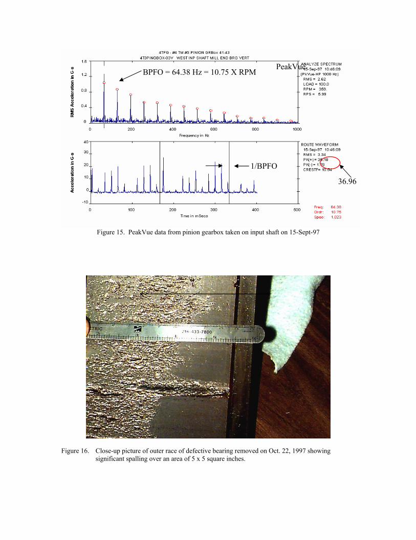
Figure 15. PeakVue data from pinion gearbox taken on input shaft on 15-Sept-97
Figure 16. Close-up picture of outer race of defective bearing removed on Oct. 22, 1997 showing significant spalling over an area of 5 x 5 square inches.
BPFO = 64.38 Hz = 10.75 X RPM
1/BPFO
36.96
PeakVue
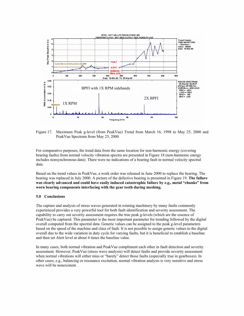
Figure 17. Maximum Peak g-level (from PeakVue) Trend from March 16, 1998 to May 25, 2000 and PeakVue Spectrum from May 25, 2000
For comparative purposes, the trend data from the same location for non-harmonic energy (covering bearing faults) from normal velocity vibration spectra are presented in Figure 18 (non-harmonic energy includes nonsynchronous data). There were no indications of a bearing fault in normal velocity spectral data. Based on the trend values in PeakVue, a work order was released in June 2000 to replace the bearing. The bearing was replaced in July 2000. A picture of the defective bearing is presented in Figure 19. The failure was clearly advanced and could have easily induced catastrophic failure by e.g., metal “chunks” from worn bearing components interfacing with the gear teeth during meshing. 5.0 Conclusions The capture and analysis of stress waves generated in rotating machinery by many faults commonly experienced provides a very powerful tool for both fault identification and severity assessment. The capability to carry out severity assessment requires the true peak g-levels (which are the essence of PeakVue) be captured. This parameter is the most important parameter for trending followed by the digital overall computed from the spectral data. Generic values can be assigned to the peak g-level parameters based on the speed of the machine and class of fault. It is not possible to assign generic values to the digital overall due to the wide variation in duty cycle for varying faults, but it is beneficial to establish a baseline and then set Alert level at about 4 times the baseline value. In many cases, both normal vibration and PeakVue compliment each other in fault detection and severity assessment. However, PeakVue (stress wave analysis) will detect faults and provide severity assessment when normal vibrations will either miss or “barely” detect those faults (especially true in gearboxes). In other cases, e.g., balancing or resonance excitation, normal vibration analysis is very sensitive and stress wave will be nonexistent.
BPFI with 1X RPM sidebands
2X BPFI 1X RPM
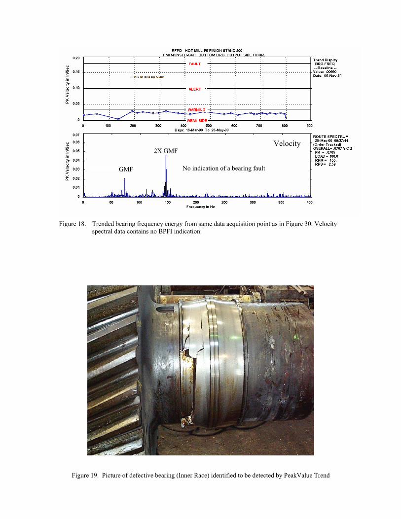
Figure 18. Trended bearing frequency energy from same data acquisition point as in Figure 30. Velocity
spectral data contains no BPFI indication.
Figure 19. Picture of defective bearing (Inner Race) identified to be detected by PeakValue Trend
No indication of a bearing fault GMF
2X GMFVelocity


