

Laser Heating and Destruction of
Carbon Nanotubes
Marc Villà Montero
Supervision:
Pr. Alexander Soldatov and Maxime Noël
High Pressure Spectroscopy Group
Luleå University of Technology

Laser Heating and Destruction of CNTs Marc Villà Montero
1
In memoriam Andreu Mont Sancho Barcelona, 3rd of October 2013

Laser Heating and Destruction of CNTs Marc Villà Montero
2
Acknowledgements I would like to thank professor Alexander Soldatov for all the wise advises he gave me during the project course and for encouraging me to keep on working to achieve all objectives. I am also very grateful to the supervisor of this project, Maxime Noël, PhD student in the division of Physics, who supported me in my work and guided me during the semester. Working with him has been a great pleasure and I had the chance to learn a lot from him, since he did several previous studies regarding the same topic. Moreover, I really appreciate the help and explanations provided by the soon to be doctor Mattias Mases. His experience on the domain was useful to finally achieve a huge knowledge of the behaviour of carbon nanotubes under high temperature. Furthermore, the advises from Doctor Ivan Evdokimov, Postdoctoral research fellow in the division of Physics, as well as the PhD student Vicente Benavides, were always interesting. I want to thank as well my colleagues Juhan Lee and Vincent Gillet. All the discussions with them made me progress faster on the project.
Laser Heating and Destruction of CNTs Marc Villà Montero
3
Table of Contents INTRODUCTION .................................................................................................................................................... 4
1. CARBON-‐BASED NANOMATERIALS ....................................................................................................... 5 1.1. THE CARBON BOND ..................................................................................................................................................... 5 1.2. GRAPHENE .................................................................................................................................................................... 5 1.3. FULLERENES ................................................................................................................................................................. 6 1.4. CARBON NANOTUBES ................................................................................................................................................. 8 1.4.1. Structure and notation ................................................................................................................................... 8 1.4.2. Thermal Properties of CNTs ....................................................................................................................... 10 1.4.3. Elastic properties of CNTs ........................................................................................................................... 12 1.4.4. Water filled carbon nanotubes ................................................................................................................. 13
2. RAMAN SPECTROSCOPY ........................................................................................................................ 14 2.1. THE PRINCIPLE ......................................................................................................................................................... 14 2.2. RAMAN SPECTRUM IN SWCNTS ............................................................................................................................ 15 2.3. HEATING EFFECTS IN THE RAMAN SPECTRA ........................................................................................................ 19
3. EQUIPMENT AND SOFTWARE .............................................................................................................. 20 3.1. EQUIPMENT IN THE LAB .......................................................................................................................................... 20 3.2. SENTERRA RAMAN MICROSCOPE ........................................................................................................................... 21 3.3. WITEC SYSTEM ........................................................................................................................................................ 21 3.4. SOFTWARE ................................................................................................................................................................. 22 3.4.1. OriginLab ........................................................................................................................................................... 22 3.4.2. PeakFit ................................................................................................................................................................ 22
4. CHARACTERISATION .............................................................................................................................. 23 4.1. EXPECTED INFORMATION ........................................................................................................................................ 24 4.2. SAMPLE PREPARATION ............................................................................................................................................ 25 4.3. CHARACTERISATION TESTS .................................................................................................................................... 25 4.3.1. Red Laser ............................................................................................................................................................ 26 4.3.2. Green Laser ....................................................................................................................................................... 33 4.3.3. Peak-‐width and peak-‐intensity studies ................................................................................................. 40
4.4. RESULTS AND CONCLUSIONS ................................................................................................................................... 43 4.4.1. Red Laser results ............................................................................................................................................. 43 4.4.2. Green Laser results for shift studies ....................................................................................................... 45 4.4.3. Conclusions ........................................................................................................................................................ 47
5. LASER HEATING EXPERIMENT ............................................................................................................ 48 5.1. INTRODUCTION ......................................................................................................................................................... 48 5.2. EXPERIMENTAL PLANNING ..................................................................................................................................... 48 5.2.1. Expected planning .......................................................................................................................................... 48 5.2.2. Final planning .................................................................................................................................................. 50
5.3. EXPERIMENTAL METHOD ........................................................................................................................................ 51 5.4. PREVIOUS RESULTS .................................................................................................................................................. 53 5.5. PRELIMINARY WORK ................................................................................................................................................ 56 5.5.1. Sample and material preparation .......................................................................................................... 56 5.5.2. Calibrations ....................................................................................................................................................... 56
5.6. RESULTS ..................................................................................................................................................................... 60 5.6.1. First results ........................................................................................................................................................ 60 5.6.2. Final results ....................................................................................................................................................... 64
5.7. CONCLUSION .............................................................................................................................................................. 66 5.8. FUTURE STUDIES ...................................................................................................................................................... 69
REFERENCES ....................................................................................................................................................... 70
TABLE OF FIGURES ........................................................................................................................................... 72
TABLES SUMMARY ............................................................................................................................................ 74
APPENDIXES ....................................................................................................................................................... 74

Laser Heating and Destruction of CNTs Marc Villà Montero
4
Introduction Research on carbon materials is, nowadays, the most developed field within the nanotechnology. Graphene and carbon nanotubes (CNTs) are the materials studied the most in this domain due to their astonishing mechanical, thermal, structural and electrical properties. They are expected to be the materials used mostly in the future thanks to their appealing properties. A lot of research for the synthesis of new advanced composite materials in a wide range of applications is developed. Nevertheless, the research and study of these materials has started only 15 years ago, so there is still a long path to go through. Before starting to think about direct applications of CNTs, basic research needs to be done in order to understand the fundamental properties. A very good tool to study CNTs is the Raman Spectroscopy, which has been used in order to characterise them. It has been observed that the laser used in Raman Spectroscopy can damage the CNTs. In this project, by using laser during Raman measurements, thermal properties of CNTs has been studied at low power density (LPD) and high power density (HPD). These studies will help for a better understanding of thermal properties of CNTs as well as future methods of purification and functionalization.

Laser Heating and Destruction of CNTs Marc Villà Montero
5
1. Carbon-‐based nanomaterials
1.1. The carbon bond Carbon is a basic element present everywhere in our planet. Its binding capabilities make carbon a very interesting material to be studied. In fact, one of the branches of chemistry is based on the ability of carbon to create bonds between other elements: the organic chemistry. Six electrons, shared evenly between 1s, 2s and 2p orbitals (1s22s22p2), surround carbon atoms. The promotion of the 2s electrons to one ore more 2p orbitals creates covalent bonds. Depending on how many p orbitals are involved, we can find three kinds of hybridization:
-‐ First type: 2s orbital hybridizing with one 2p orbital forming two orthogonal sp1 (180°) orbitals.
-‐ Second type: 2s orbital hybridizing with two 2p orbitals forming three sp2 plane (120°) orbitals (graphene).
-‐ Third type: 2s orbital hybridizing with the three 2p orbitals forming four sp3 tetragonal (109.5°) orbitals.
In dependence of the hybridization of the carbon orbitals, carbon can bind σ and π bonds. Well-‐hybridized orbitals form σ-‐bonds, which are strong bonds, like in the diamond orbitals, where orbital in all atoms are sp3 hybridized and form four σ-‐bonds in a tetragonal structure. On the other hand, unhybridized orbitals from weak π-‐bonds. The strength of σ-‐bonds gives carbon the possibility to form complex pure structures, such as diamond, graphite and fullerene also known as allotropic forms of carbon [1].
1.2. Graphene Graphene was studied by accident in 2004, while some physicists from the University of Manchester were trying to produce thin films out of graphite. Graphene is basically a layer of carbon in sp2 configuration, forming three in-‐planar bonds with a 120° angle separation between them. It can be considered as a 2-‐D structure. Carbon atoms form a hexagon crystal lattice similar to a one atom thick honeycomb. The simplest building block in graphene, which is also known as Brillouin zone, is the hexagon that forms the honeycomb structure.

Laser Heating and Destruction of CNTs Marc Villà Montero
6
Graphene structure has some similarities with the one from graphite. Graphite can be considered as a pile of graphene sheets (at least 5), where each carbon atom bonds with three other carbon atoms in the same plane by using 120° σ-‐bonds, just like the structure found in graphene. Then, the fourth free electron of the each carbon binds with the electrons of the other layers by using weak π-‐bonds. The point is that these delocalised electrons have free movement within the sheet; each electron is no longer fixed to a particular carbon atom [2]. Above ten layers of graphene can form thin layers of graphite and a bulk of graphite can be formed when the number of layers reaches infinity. In the case of graphene, π-‐bonds are left out of plane, what leads to an exceptional electron mobility and corresponding low resistivity, even lower than silver if it is properly isolated. However, electron scattering decreases the electron mobility and increases the resistivity due to phonon interaction from contact surfaces at room temperature. Graphene is seen as one of the strongest material with a breaking strength 200 times greater than steel and, also, better thermal conductor than diamond. A possible defect on graphene hexagon sheet is the presence of different geometrical forms; for example, heptagon forms bend the plane turning it to a saddle shape. On the other hand, presence of pentagons results in a cone shape. More pentagons will increase the curvature until the point that the sheet can be transformed to a closed shape.
1.3. Fullerenes Rick Smalley and co-‐workers discovered Fullerenes in 1985. Fullerenes are the third allotrope of carbon and they consist of a closed shape molecules. The sp2 orbitals become more sp3 due to the curvature of the graphene sheet, then the degree of hybridisation, spn, becomes non-‐integer, with 2<n<3. The shape can be spheroidal or cylindrical. The tubular form of fullerenes, nanotubes, will be the subject of study of this project. Fullerenes are also known as buckminsterfullerenes. The first form discovered was a C60 or “buckyball”, which is like a soccer ball composed by 60 carbon atoms bonded together in twelve pentagons and twenty hexagons arranged to form a truncated icosahedron. Like in graphite and graphene, the atoms are sp2 hybridized, but in this case, they are not arranged on a plane, due to the presence of pentagonal structures. It was discovered by accident, like many other scientific breakthroughs while a team of scientists was studying interstellar dust, the long-‐
Laser Heating and Destruction of CNTs Marc Villà Montero
7
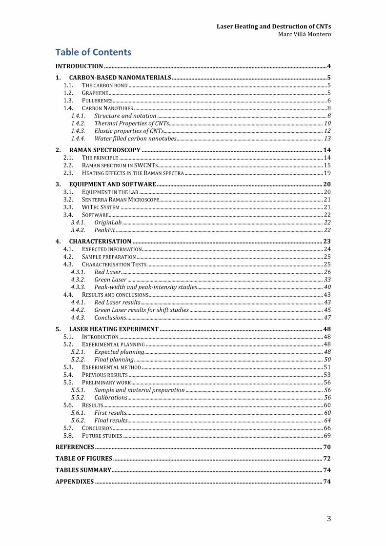
chain polyynes formed by red giant stars, by experimenting with graphite [1]. Later, other Cn structures were discovered, such as C70. In 1990, Rick Smalley proposed the existence of tubular fullerene. Carbon nanotubes are generally one or few nanometres in diameter, hence the name nanotubes, and many micrometres in length. In this case they are considered as 1D material. Sometimes the tube is so short that adapts a spherical shape. These kinds of nanotubes are also called Buckyballs and are considered 0-‐D materials. The International Union of Pure and Applied Chemistry (IUPAC) firstly established a nomenclature for the fullerenes in 1997. In that report, the definition of fullerene was too strict and, it basically only accepted fullerenes under closed-‐cage structures with 12 isolated five-‐membered rings and only spherical an ellipsoidal shapes [3]. Later, in 2002, a more updated and less restrictive nomenclature was released also by the IUPAC. This current nomenclature accepts closed carbon nanotubes, nanotourses and many other closed cage structures [4]. In summary, CNTs can be considered as a kind of fullerenes. Since CNTs is the material studied along this project, in the following part, CNTs’ structure such as its properties will be widely explained. There exist different ways to produce fullerenes and CNTs, even by burning a candle we can produce a little amount of fullerenes [5] or by vaporisation of graphite in an inert atmosphere [6].
Figure 1.1. Schematic representation of a graphene sheet (top-‐left), graphite (top-‐right), SWCNT
(bottom-‐left), fullerene (bottom-‐right) [20]

Laser Heating and Destruction of CNTs Marc Villà Montero
8
1.4. Carbon Nanotubes The aim of this project is to study single-‐walled carbon nanotubes under extreme heating conditions, induced by the laser beam during Raman spectroscopy. Two kinds of single walled nanotubes will be used: empty CNTs and water filled CNTs, with water molecules inside them. In order to be able to interpret the results obtained, firstly it is needed to understand CNTs structure and properties.
1.4.1. Structure and notation Even if CNTs are considered as fullerenes, a CNT can be also seen like a graphene single sheet rolled up into a seamless cylinder. Firstly it was thought that only multi-‐walled carbon nanotubes (MWCNTs) existed, later it was discovered the existence of single-‐walled carbon nanotubes (SWCNTs). These tubes measure some nanometres in diameter. On length they measure over some micrometres and in some cases millimetres. Due to its small diameter over length ratio they are considered 1-‐D materials [7]. As mentioned, CNTs can be contained in other CNTs. When only one CNT is in another CNT it is called double-‐walled carbon nanotube (DWCNTs). If we find more that two CNTs or the graphene sheet is rolled several laps into Swiss roll shape, then they are called MWCNTs. To understand CNTs we first need to know its structure. As said before, CNTs can be studied as a rolled graphene sheet. The graphene plane can be labelled with vectors, Ch and T, whose rectangle define the unit cell. Ch defines the circumference on the surface of the connecting two equivalent atoms. This vector can be defined as (1.1). 𝐶! = 𝑛𝑎! +𝑚𝑎! (1.1)
Figure 1.2. Schematic representation of Ch vector and the basis vectors of graphite [24]
âx represent the two basis vectors of graphite (figure 1.2) and n and m are integers that determine the chiral angle (2.2). In figure 1.3, we can see a graphical representation of this angle. The chirality angle range is in between 0° and 30°.

Laser Heating and Destruction of CNTs Marc Villà Montero
9
𝜃 = 𝑡𝑎𝑛!! 3𝑛
2𝑚 + 𝑛 (1.2)
Figure 1.3. In green, Ch vector, in red, armchair section and in bold black zig-‐zag structure [23]
By only using the integers of the Ch, it is possible to have all the information regarding the CNT structure. The following notation is adapted to refer to all CNTs. 𝐶 = (𝑚,𝑛) (1.3) The carbon nanotubes are rolled on the way that the Ch vector is contained along the CNT surface, parallel to the axe. The chiral angle is used to separate CNTs into three classes (figure 1.4) differentiated by their electronic properties:
-‐ Armchair (n=m, 𝜃=30°): they are considered as metallic, which means it has a zero band gap.
-‐ Zig-‐zag (m=0, n>0, 𝜃=0°): having the shape in bold black in figure 1.3 when it is opened.
-‐ Chiral (0<|m|<n, 0°<𝜃<30°)
Figure 1.4. Structure of each class of CNT [25]
The chirality plays an important role in the CNTs properties. Zig-‐Zag and Chiral CNTs can be semimetals or semiconductors. They are considered semimetals when

Laser Heating and Destruction of CNTs Marc Villà Montero
10
n-‐m/3=i (i being integer and m≠n), and they own a finite band gap. In any other case, they are considered semiconductors. The band gap for semiconductor and semi-‐metallic nanotubes is about the inverse of the tube diameter (1.4). That gives to each carbon nanotube a unique electronic behaviour [8].
𝑑! = 3𝑎!!!𝑚! +𝑚𝑛 + 𝑛!
𝜋 =𝐶!𝜋
(1.4)
Where Ch is the length of the vector and ac-‐c is the C-‐C bond length (1.42 Å). The combination of different diameters and chiralities leads to hundred individual kind of nanotubes with different properties. Isolated SWCNTs have promising properties regarding strength and conductivity of heat and electricity. However, it is very difficult to get isolated SWCNTs. Bulk CNTs usually consist in a mix of semiconducting and metallic nanotubes that interact with one another through Van der Waals bonds, which makes its properties less attractive. To find a way to maintain these good properties in a bulk of CNTs, is one of the targets of all CNT researcher.
1.4.2. Thermal Properties of CNTs Carbon allotropes and their derivatives occupy a unique place in terms of their ability to conduct heat. They have a very good behaviour regarding the thermal conductivity at room temperature. The highest thermal conductivity range is observed in CNTs and graphene what makes them useful in terms of thermal management of electronics. Thermal conductivity is measured as K, which is a constant value at low temperature. At wide temperature range, K is a function of temperature. To have a global idea, in pure cooper, one of the best metallic heat conductors, thermal conductivity reaches K≈400 Wmk-‐1. In the case of solid materials, heat is carried through phonons (Kp), that excites the crystal lattice making it vibrate, and electrons (Ke), which dominates in heat conduction in metals. In the case of carbon materials, heat conduction is dominated by phonons (KP), even for graphite, which have metal-‐like properties. That property is due to the strong sp2 bond resulting in efficient heat transfer by lattice vibration.

Laser Heating and Destruction of CNTs Marc Villà Montero
11
Carbon based materials have been rigorously studied along the last century. Graphite can have thermal conductivities from 200 to 2000 Wmk-‐1, which is a very big range, depending on the production technique or the crystalline structure. In bulk carbon allotropes, heat is carried by acoustic phonons. Regarding thermal transport in CNTs and graphene, the heat transport is carried out through the strong sp2 lattice, what gives very high K values. The fact that CNTs are cylindrical makes them have different quantization conditions for phonon modes than graphene. A very interesting property observed in CNTs heat transport is the ballistic transport regime. This phenomenon can be explained as the phenomenon that happens while transporting light through optical fiber. The heat goes through the CNT without any obstacle. Ballistic transport regime can lead to very high K values (K≈3000 Wmk-‐1 at room temperature). It is not always observed, what leaves a wide range of thermal conductivity constants regarding all kind of CNTs (table 1.1). SWCNTs have better thermal transport properties than other kinds of nanotubes, reaching values of K≈7000 Wmk-‐1 at room temperature. Nevertheless, graphene is the best heat conductor ever discovered at the present day. In some papers they talk about values of heat transport constant of 10,000 Wmk-‐1 at room temperature [9]. In table 1.1, information about experimental data, from graphene, SWCNT and CNT, is given jointly with information regarding the method used to calculate each value.

Laser Heating and Destruction of CNTs Marc Villà Montero
12
Table 1.1. Thermal conductivity of graphene and CNTs [10]
When the CNTs tested are in state of bundles the thermal properties decrease substantially. In this project the CNTs will be heated by means of a laser beam, this will decrease thermal properties and, moreover, can cause its destruction [11].
1.4.3. Elastic properties of CNTs Even working on the nanoscale, we can attempt to describe the mechanical properties of CNTs in a continuum approach. There are some experiments that can give information about the stress-‐strain relationship, for example, bending, indentation or resonantly vibrating beam experiments (Raman spectroscopy) [12]. Young moduli of SWCNTs bundles can be also determined by high-‐resolution transmission electron microscopy (HRTEM) and atomic force microscope (AFM). CNTs have very high strength, flexibility and resilience. In terms of mechanical properties, carbon nanotubes are more focused on improving the properties of composite materials and reinforcements. Experiments done by J. Salvetat [22] et al. shown that CNTs have at least the same Young’s modulus as graphite (1000 GPa) and in the case of small SWCNTs, the modulus is even higher. It was also shown that the Young’s modulus decrease as the disorder in the CNT structure increases (figure 1.5).

Laser Heating and Destruction of CNTs Marc Villà Montero
13
Figure 1.5. Modulus vs. Disorder in MWCNTs [22]
The point of study of the mechanical properties of CNTs is focused on the composite materials, thanks to the good load transfer between polymer matrices and CNTs surface, so the extraordinary properties of CNTs can be reflected on the composite.
1.4.4. Water filled carbon nanotubes It has been demonstrated that water can fit into SWCNTs lattice despite of the hydrophobic properties of its walls, and even a very fast transport can be produced [13]. Water can fit in SWCNTs even in very thin diameter samples, such as d≈5 nm. In that case, only a molecule of water can fit inside the nanotube channel [14]. To prove water filling CNTs microscopy techniques and electron microscopy can be used. To obtain other information regarding the diameters and chiralities of the CNTs other techniques such as Raman Spectroscopy or neutron scattering are used. It has been theoretically demonstrated that water-‐filled SWCNTs experiment upshifts in the radial breathing mode (RBM) of 2-‐6 cm-‐1, what makes Raman spectroscopy a good way to also prove water filling in CNTs by using resonant Raman scattering [15]. Empty individual SWCNTs have reduced extrinsic perturbations, resulting in narrow emission lines in the RBM for small diameters [16]. The fact that only a single water molecules fits inside the tube is a promising property in terms of ultrafiltration applications. Water-‐filling SWCNTs may also improve their mechanical resistance to high pressure [13].

Laser Heating and Destruction of CNTs Marc Villà Montero
14
2. Raman Spectroscopy Raman spectroscopy allows us to study the low frequency levels in a system or a structure without sample preparation [17]. Each molecule on a system has different energy levels. This property makes Raman spectroscopy a useful tool to identify precisely the nature of a sample. It can provide information on the chemical structure and physical forms or it can be used to determine quantitatively the amount of substance in the sample [18]. The Indian physicist Sir Chandrasekhara Venkata Raman discovered this technique in 1928. Two years later, he was awarded the Nobel Prize for his findings.
2.1. The principle The principle is to rely on an inelastic scattering (Raman scattering) of monochromatic light, which can be, for example, a visible laser beam, to the vibrational modes of a system. The laser light excites the molecules and makes them vibrate resulting in the energy of the laser photons being shifted up or down. That shift gives information about the vibration modes of the system. Normally a laser beam is used to excite the molecules. The studies of this project will be done with red (1.96 eV) and green (2,33 eV) lasers. This radiation is called excitatory. The laser beam impacts on the sample and its photons can be reflected or absorbed. A small fraction of the light is scatted in all directions. This light scatted is the point of study of this technique. The majority of this light scatted has the same frequency (ν0) as the excitatory radiation from the laser. That scattering without any frequency change is called Rayleight scattering (figure 2.1). A very few quantity of this light (less than 1/1000) is scattered on a different frequency (νd) than the excitatory radiation. If this frequency is bigger than the excitatory radiation, it is obtained the Raman anti-‐Stokes scattering. If the opposite scenario is given, the Roman Stokes scattering is obtained (2.1). 𝜐! < 𝜐! ; 𝜐! = 𝜐! − 𝜐! 𝑅𝑎𝑚𝑎𝑛 𝑆𝑡𝑜𝑘𝑒𝑠 𝑠𝑐𝑎𝑡𝑡𝑒𝑟𝑖𝑛𝑔
𝜐! > 𝜐! ; 𝜐! = 𝜐! + 𝜐! 𝑅𝑎𝑚𝑎𝑛 𝐴𝑛𝑡𝑖 − 𝑆𝑡𝑜𝑘𝑒𝑠 𝑠𝑐𝑎𝑡𝑡𝑒𝑟𝑖𝑛𝑔 (2.1)

Laser Heating and Destruction of CNTs Marc Villà Montero
15
The point of study is the gap of frequency νv, which is equal to the Raman active vibrations of the studied sample. This Raman spectrum contains information that can be useful for study.
Figure 2.1. Interaction between a photon and matter characterised by energy states
The photons are collected and transformed to an electrical signal, which later on is transformed to the corresponding Raman spectrum. Normally the Stokes band is more intense than the anti-‐Stokes one and the Rayleigh band is filtered out before the detector. To talk about the frequency of radiation normally it is used another number: the wave number (2.2), where c is the celerity of light (3.108 m·s-‐1) and 𝜆 is the wavelength. 𝜐 =
𝜐𝑐 =
1𝜆
(2.2)
The units of the wavenumber are cm-‐1 and sometimes it is called Kayser. In all Raman signals, the frequency of radiation is expressed as the wave number. The wavenumber is also inversely proportional to the CNT diameter. Raman-‐active vibrations or rotations in molecules give a spectrum that shows different peaks of different frequencies and intensities. For carbon-‐based materials the spectra have some well-‐defined peaks that allow us to study them. Moreover, in the case of SWCNTs, a peak under a wave number of 100-‐250 cm-‐1 is observed. This peak will be the one of the subjects of study of this project.
2.2. Raman spectrum in SWCNTs To characterise the peaks of the spectrum the 𝜐! is used instead of 𝜐! and it does not depends on the choice of the excitation frequency (𝜐!). This number is equal to the range between the Raman peak and the Rayleigh peak and it is called relative

Laser Heating and Destruction of CNTs Marc Villà Montero
16
wave number. The wavenumber used is shown in figure 2.2 and would be, for example, the wavenumber distance between the Rayleigh scattering (green) and some other peak.
Figure 2.2. Spectrum example showing the different scatterings as a function of the wavenumber and
wavelength [19]
As said before, the Raman spectra in SWCNTs have some particular peaks. Normally there are four main features that are always observed under the same range of wavelength (figure 2.3)
-‐ Radial Breathing Mode (RBM): It is normally observed in between 100-‐300 cm-‐1. It is due to radial movement of the atoms while the SWCNTs are excited. It is a characteristic peak on SWCNTs assigned to a breathing mode of the tubes. It is inversely dependent on the diameter of the tube [17]. Its absence can mean the destruction or absence of the SWCNTs. With diameters greater than 2 nm, the intensity of this peak is weak.
-‐ D-‐band: It is normally observed at ~1350 cm-‐1. Its intensity depends on the defects on the CNTs surface. It is assigned to residual ill-‐organised graphite. The different forms of carbon can be appreciated by the position and linewidth of the band. To have an idea, SWCNTs show a characteristic linewidth of 10-‐30 cm-‐1, thinner for graphite (30-‐60 cm-‐1).
-‐ G-‐band: It is normally observed at ~1590 cm-‐1 and gives information about the plane movements of the atoms. It is related to shear stresses. It is also a characteristic of CNTs. This band is usually composed of 6 peaks, where only two are useful for analysis: the lower and the higher frequencies, G-‐ and G+ respectively. They are associated to the displacements of the atoms the circumferential direction and the axis. This band can be used to study

Laser Heating and Destruction of CNTs Marc Villà Montero
17
the diameters and the metallic/semiconducting properties of the CNTs although the information obtained is less accurate than that from RBM. Semiconducting CNTs show a narrow G-‐band, whereas, for metallic CNTs, the G-‐ band is wide and asymmetric.
-‐ G’-‐band: It is a second order observed mode at very high wavenumber (~2650 cm-‐1). Like the D-‐band, the G’-‐band gives information about defects on the CNTs, but in this case the defects are from the inside of the CNTs.
It can be observed a second order mode band. It is something predicted for infinite and homogenous bundles of SWCNTs with a radii greater than 0.7 nm. The larger the radii, the lower the second order mode is. If the CNTs are placed on a silicon substrate, a band produced by the glass can appear after the RBM band.
Figure 2.3. Raman spectrum showing the principal characteristics of CNTs. Spectrum obtained from and
individualised SWCNTs with diameter about 1.07nm, using a E=1.16 eV laser [17]
The subject of study in this project will be generally the RBM and the G-‐band because all the information regarding the CNTs degradation leads there. While degradation, the RBM shows an intensity decrease whereas the G-‐band shifts some cm-‐1. It is difficult to isolate properly a SWCNT in order to study it. In the most of the cases, a bundle of SWCNTs is studied. In this case, it can be tricky to interpret

Laser Heating and Destruction of CNTs Marc Villà Montero
18
correctly the results. For example, in the RBM it could be observed more than one peak in different wavenumber. That may be due to the presence of different sizes of SWCNT. The only visible CNTs in the Raman spectrum are those that have the same transition energy as the excitation energy because in that case, this energy coincides enhance the Raman signal. The technique is then called Resonance Raman spectroscopy and multiplies the signal of tubes by 106,, allowing observation of such nanoscale objects. The transition energy of the CNTs depends on its chirality. There is a way to relate the diameter of the CNTs with its electronic transition energy for different chirality: the Kataura plot (figure 2.4). In the Kataura plot it is also possible to differentiate metallic and semiconducting CNTs [21]. The Kataura plot is a useful tool to have a first idea about the parameters needed for the study of the SWCNTs.
Figure 2.4. Kataura plot for SWCNTs for 𝛾=2.75 𝑒𝑉. Solid circles indicates metallic SWCNTs and the empty
ones, semiconducting SWCNTs. The arrows show the diameter distributions of each catalyst [21]

Laser Heating and Destruction of CNTs Marc Villà Montero
19
2.3. Heating effects in the Raman spectra Analysing the Raman spectra is the best way to study the overheating effect on CNTs. When the CNTs are overheated or destructed, its vibration state changes, so the Raman spectra changes slightly. The most evident variation is observed in the G-‐band, which usually shows a downshift of the peak position. It has been proved that this downshift has a linear relationship with the temperature. While the temperature increases, the peak decreases. This downshift depends on the temperature and normally the change shift observed is about 0.01-‐0.03 cm-‐1/K depending on the CNT chirality and impurities. The standard variation considered is 0.025 cm-‐1/K [26]. In some cases a downshift in the RBM peaks can be observed. It is thought that it depends on the environment where the nanotubes are placed [26].
Figure 2.5. Evolution of the G-‐band position as function of the temperature [26]

Laser Heating and Destruction of CNTs Marc Villà Montero
20
3. Equipment and software
3.1. Equipment in the lab During this project not only spectroscopy setups used. To prepare the samples it was needed to use some standard material that can be found in every laboratory and also some more specific tools. All samples were prepared on small squared glass slides of 2 cm sides. The nanotubes were placed on the glass slide by means of a pair of laboratory tweezers. Previously, all material was cleaned using cotton sticks that were previously impregnated by ethanol 98% pure. Once the nanotubes were placed under powder form on the glass slide, distilled water was used to fix them once dried. To add the
droplet of distilled water, a pipette was used. To proceed with the heating experiments, the samples were placed in a hermetic cell. Initially it was planned to carry the experiments by using an old hermetic cell that was manufactured by the collaboration team in Nancy (Université Lorraine). After this cell broke, it was decided to use a better cell provided by the chemistry laboratory of LTU (Luleå Tekniska Universitet). This cell, also known as Linkam cell, was an easy-‐use cell especially designed for this kind of experiments. The temperature of the cell can be controlled and automated and also it is very easy to plug the inputs/outputs from the gas bottle in order to create an oxygen-‐free atmosphere. To create the argon atmosphere, a gas-‐loading system of argon gas was used and plugged to the cell. The system allows keeping a constant flow of argon in the output and in very low
Figure 3.1. Linkam temperature stage
Figure 3.2. Gas loafing system of argon used to fill the cell

Laser Heating and Destruction of CNTs Marc Villà Montero
21
pressure, which was of interest for cleaning the cell from its oxygen and filling it slowly with argon without increasing the pressure inside the cell. Besides this basic material two different spectroscopy setup were used.
3.2. Senterra Raman Microscope Senterra Raman is a high performance Raman microscope produced by Bruker® [27]. It has an auto calibration system that makes it very comfortable to work with. Senterra microscope combines the sensitivity of the dispersive Raman technology and the wavelength accuracy of the Fourier-‐transform Raman spectroscopy. It is possible to choose between different wavelengths (1064nm, 788nm, 633nm, 532nm and 488nm). It was only used for the characterisation part using green laser (532nm) due to the fact that it is less precise and it is not possible to modify the laser parameter as much as it is possible in WiTec System.
3.3. WiTec System WiTec System is a system that joints a Raman microscope with other external lasers. The microscope combines an extremely sensitive confocal microscope with an ultrahigh-‐throughput spectroscopy system for unprecedented chemical sensitivity. An efficient combination of filters, objectives and lenses used in conjunction with detectors provide the highest spatial and spectral resolution [28]. “WiTec GmbH” produces it. It can be used to detect signals from extremely low material concentration or volumes, perfect for analysing CNTs. Ruthermore, it is possible to connect different external lasers to the microscope. In the lab it is possible to use a green laser (532nm) and a red laser (633nm). It was planned to carry out
Figure 3.3. Picture of a Senterra Raman Microscope from Bruker [27]
Figure 3.4. Schema of a Raman microscope from WiTEC UHTS 300 [28]

Laser Heating and Destruction of CNTs Marc Villà Montero
22
the experiments using both lasers, but due to lack of time, they were only done using the red laser. The characterisation of the nanotubes under red laser was also done using this system. It is possible to achieve a better resolution than with Senterra Raman since it is possible to control all parameters. Differently from Senterra, the laser power is regulated from the laser and not from the software, so more exact laser powers are possible to be set.
3.4. Software In order to treat the data, the following different softwares were used besides the ones of the Raman microscopes and the Office pack.
3.4.1. OriginLab OriginLab is an easy-‐to-‐use data analysis graphing software application [29]. It has more or less the same principles as Excel. It has been used to plot all the spectra in a proper way and also to treat the data obtained from the spectroscope.
3.4.2. PeakFit PeakFit is an automated non-‐linear peak separation and analysis software package performing spectroscopy, chromatography and electrophoresis [30]. It detects automatically the peaks and then, by using Lorenz functions it is possible to modify them and make them fit. It was used to characterise the RBM signals and also to plot the results from the heating test.

Laser Heating and Destruction of CNTs Marc Villà Montero
23
4. Characterisation Before starting any tests, it was very important to know as much as possible about the nature of the material to be analysed. The nanotubes studied in this project were manufactured in Antwerp University in Belgium and delivered by the same institution in small capsules in powder form in small capsules. The information received from them was not very specific so some tests were required in order to find out more precise information about the nanotubes. Two different kinds of HiPCO nanotubes were provided: open and closed. The open tubes were supposedly water-‐filled while the closed ones were empty. In the specifications it was explained that the both, closed and open HiPCO powder samples were not 100% closed or open, but more 90% closed and 90% opened. In any case, this should be sufficient to see differences in the spectra. It has been recommended not to use sonication to prepare the samples, especially for the closed powder sample, because of the possibility of opening and damaging them. To characterise the two materials obtained only Raman Spectroscopy was used, as it will be explained in detail in a next part. First of all it was important to talk about the sample preparation and the expected information to be obtained. The characterisation was done on both types of tubes and the data was processed using OriginLab and PeakFit, in order to be able to analyse the frequencies where the peaks were observed. The main importance of such an extensive characterisation was that, differently than in previous studies [11], in this case the nanotubes were not dispersed. Now the studied nanotubes were dry and non-‐dispersed, only fixed on a glass by means of a distilled water droplet. The main difference between studying a dry bundle and dispersed nanotubes lies on the RBM profile distribution. While in dispersed nanotubes, the signal obtained in the lower frequencies has fewer peaks due to the presence of less and always-‐constant nanotube sizes; in the case of dry bundles the distribution of the nanotubes may be random. This randomness makes the RBM profile to have unpredictable peaks and, therefore, more difficult to be compared.

Laser Heating and Destruction of CNTs Marc Villà Montero
24
The purpose of the characterisation was to find out if it was possible to obtain same profiles in different bundles and in different kind of nanotubes, in order to be able to compare closed (empty) and open (water filled) CNTs.
4.1. Expected information It was expected to observe several differences between the spectra collected from open and closed tubes. Also by using different wavelengths (532 and 633nm), different families (chiralities) of nanotubes are excited. Since in this project the nanotubes were not individualised but organised within aggregates, the RBM spectra obtained must show different peaks at different frequencies. The results from open compared to closed tubes should be slightly different. Normally a shift to higher frequency and a drop of intensity in the RBM spectra in open (water-‐filled) tubes spectra is observed compared to the one from the closed tubes. Also, it was expected to observe an increase of the width. The aim of the characterisation was to find a similar RBM profile in both closed and open in order to be able to compare both materials during the tests.
Figure 4.1. Influence of water filling of SWCNTs in the RBM spectra, Red (grey) belongs to closed (empty)
tubes and blue (dark grey) corresponds to open (water-‐filled tubes) [14]

Laser Heating and Destruction of CNTs Marc Villà Montero
25
4.2. Sample preparation The only requirement for the sample preparation was not to use sonication on the closed (empty) tubes. Sonication can easily damage the closed nanotubes by opening them. This opening will lead to the filling of the tubes and make same identical to the water-‐filled tubes. Since the aim is to obtain similar spectra from both types of tubes, it was decided not to use sonication to prepare the open HiPCO samples neither. Samples were prepared using a distilled water droplet onto HiPCO powder placed on a glass slide. Firstly using ethanol and earplugs, all the material was carefully cleaned. The carbon nanotubes were placed on the glass slide by using tweezers. It was not needed to place a lot of powder, only the amounts needed to be able to differentiate some aggregates with a naked eye. Once the particles were placed on the glass slide, a droplet of distilled water was added over the nanotubes grains by means of a pipette. Afterwards, the sample was left in a dry place to let it dry for over 2 hours. The main reason of applying the droplet was to fix the nanotubes on the glass slide preventing them to fly away or move. In the case of the open tubes, the droplet also acted as a water-‐filler. During the sample preparation it was very important to take care of health. It has been proved that nanoparticles can be harmful for the human body. Due to its size, the human body cannot assimilate them, so they remain in the body increasing the probability of developing diseases such as cancer. The sample preparation method for the overheating tests, done during the project, was exactly the same as the one done for the characterisation process.
4.3. Characterisation Tests Since the tests were planned to be done under red and green laser, the characterisation was done under the same conditions in order to know what kind of spectra expect for both types lasers. Different wavelength allows us to detect different families of CNTs. That is the point of studying the nanotubes by using different lasers.

Laser Heating and Destruction of CNTs Marc Villà Montero
26
Also the characterisation was carried out for both types of nanotubes so afterwards it was possible to compare them and analyse the data. The method used to characterise was the same for both lasers and both tubes. Different aggregates were studied and, within each aggregate, several spots were analysed. The number of spots analysed depended on the aggregate size. In the case of big aggregates, a bigger number of spots were checked. The main objective of this characterisation was to find similar RBM spectra in both types of nanotubes in each kind of laser. Similar spectra don’t mean exactly the same spectra but similar characteristic peaks and same frequencies (Raman shift) with a slight shift to the right in the spectra of the water filled HiPCO compared to the empty ones.
4.3.1. Red Laser Red laser has a wavelength of 633 nm and its excitation energy is about 1.96 eV. The characterisation by using red laser was carried out using the WiTec System placed in the department of Materials Engineering at LTU. The system has a maximum resolution of 1800 gr/mm what leads a accuracy of ±0.59 cm-‐1. The tests were run using a 100x Olympus objective (Olympus UMPlanFI 100x/0.95) under a laser power of 0.49 mW in the fiber. The drawback of using this objective is the difficulty to focus the proper surface of the sample, but its accuracy was a big advantage. First of all, several spectra of the G-‐band were taken in order to find out the Reference Spectrum, which is the spectrum taken at the maximum temperature the nanotubes can bore without being overheated. This spectrum is used to compare non-‐tested nanotubes with overheated ones and also indicates the maximum laser power usable for the characterisation process. To find the reference spectrum, some low-‐resolution spectra were collected while increasing the laser power starting with a very low one. All the spectra were collected in the same spot so it was easier to observe a shift when it occurred. After comparing different laser powers up to 0.54mW, it was observed that the highest laser power that could be used to study the closed nanotubes was 0.47mW.

Laser Heating and Destruction of CNTs Marc Villà Montero
27
The same tests were done in order to know the nature for the water-‐filled nanotubes. In this case it was observed that after 0.45mW the nanotubes started to overheat. Comparing the two values, it was decided to use for both studies (closed and open tubes) a maximum laser power of 0.45mW. Normally it would be expected to observe a lower heat resistance on water-‐filled CNTs due to the presence of oxygen molecules that increase the oxidation of the material. This did not happen this time but it was not a big issue. In the WiTec system it was complicated to have 100% control on the laser power used due to the fact that the red laser is manually adjusted and also the laser power is not always stable, so the power values utilised were not very accurate. A first characterisation using red laser was done but the parameters used were not appropriate. The results obtained were very noisy and not clear. It was difficult to differentiate between a true RBM-‐peak and noise peaks. The main reason was that the integration time selected was not enough and the Raman Spectroscope was not able to collect enough signals from the RBM. Also with a higher number of accumulations, the results would have been better. It was learnt that 3-‐5 seconds of integration time were not enough to collect a proper analysable spectrum. In any case, that was an unexpected loss of time during the project, especially because a total of 7 aggregates and 29 spots were studied and also because every time that WiTec system was used it took a lot of time to calibrate the machine before starting to run experiments.
Figure 4.2. Bad quality RBM spectra due to bad settings. At the left side, RBM spectrum from Open HiPCO using 5s integration time and 12 accumulations. At the right side, RBM spectrum from Closed HiPCO
using 3s integration time and 10 accumulations

Laser Heating and Destruction of CNTs Marc Villà Montero
28
After realising that the spectra quality was not good enough to draw serious conclusions about RBM profiles, the same characterisation was done once again, and in this case with more experience and more clear objectives and, of course, improved parameters.
4.3.1.1. Closed HiPCO (Empty) In this case the spectra were done using 90 accumulations and 10s of integration time, so the data collection lasted 15 minutes. Then, the results obtained were much better. A total of 4 aggregates and 14 spots were studied and PeakFitted and repeated a RBM spectrum was observed (figure 4.3). The data obtained from the aggregate 1 was not very accurate since it was the first aggregate to be analysed and the parameters were not completely optimised. On the other hand, for aggregates 2, 3 and 4, the spectra show some characteristic peaks that can be studied jointly with the data obtained from the open HiPCO samples.
Figure 4.3. Spectra collection corresponding to the Red laser characterisation of Closed HiPCO nanotubes

Laser Heating and Destruction of CNTs Marc Villà Montero
29
In all spectra, there were always 11 characteristic peaks that were clearly observed and used while doing the PeakFit analysis. In some cases there were also observed peaks in other frequencies. Characteristics peaks were statistically studied and, later on, compared with the characteristic peaks from the open samples.
Figure 4.4. Characteristic peaks observed under red laser
During the study of the spectra, a total of 11 peaks were reported. The lowest frequency observed was over 160cm-‐1 and the highest one was over 325cm-‐1. By using Kataura Plot, it is possible to get an approximated value of the diameters of the nanotubes, which in the case of using Red Laser was between 0.83 to 1.6 nm.
Peak number Average Standard Dev. Only in Closed HiPCO 176,27 1,73
1 192,3729 1,14 2 216,36 0,80 3 232,17 3,29 4 242,45 0,72 5 250,375 0,65 6 256,10 0,44 7 259,90 1,15 8 281,17 0,54
Only in Closed HiPCO 294,4 0,97 Only In Closed HiPCO 306,36 1,25
Table 4.1. Observed peaks in the RBM from closed HiPCO tubes under Red Laser. Each average was obtained by analysing all spots

Laser Heating and Destruction of CNTs Marc Villà Montero
30
Even though there were 11 characteristic peaks observed, only 8 of them were taken into account in order to be able to compare them with the characteristic peaks from the open tubes. All average values were calculated from all the spectra collected from each spot and, as it can be observed on their standard deviation value, there existed a good homogeneity on the data.
Figure 4.5. Plot representing the peak position of each characteristic peak and its error in the closed
HiPCO tubes under Red Laser
The standard deviation observed for peak number 3 (232 cm-‐1) was the biggest observed in this case but that could be due to the presence of data from the Aggregate 1, which at some points was not as much accurate as it should be.
4.3.1.2. Open HiPCO (Water-‐Filled) The spectra collection of the open HiPCO samples was done after the collection of the closed HiPCO samples. Since the parameters used then were good enough to get a proper spectrum, they were not modified this time. Due to time limitation and problems of finding good RBM signal by using the 100x objective, only 3 aggregates and 11 spots were analysed. It was tried to study mainly big aggregates, since it was expected to see more different nanotube sizes distribution in big aggregates than in small ones. In this case, not only a bigger amount of nanotubes sizes was observed, but also open and closed tubes were distinguished.
190
210
230
250
270
290
1 2 3 4 5 6 7 8
Raman Shift (cm
-‐1)
Peak number
Closed HiPCO -‐ peak position

Laser Heating and Destruction of CNTs Marc Villà Montero
31
It was possible to observe in a same RBM, the same exact peak observed during the characterisation of closed HiPCO next to the shifted one due to water filling. That was quite an interesting result but also unexpected to observe. The explanation of these results is due to the fact that not all CNTs from the open HiPCO powder were open and neither all the open tubes were water-‐filled. The RBM spectra from open tubes was sometimes more difficult to study because of that large amount of peaks observed.
Figure 4.6. Spectra collection corresponding to the Red laser characterisation of Open HiPCO nanotubes
In this case, only 8 characteristic peaks were found. It was more difficult to find characteristic peaks due to the proximity between peaks from open tubes and the ones from closed tubes. It was possible to compare the position of these 8 peaks in the open HiPCO RBM spectra with the ones from the closed HiPCO. Therefore, by studying a total of 8 peaks in the RBM profile, the characterisation under red laser was done.

Laser Heating and Destruction of CNTs Marc Villà Montero
32
The diameters of the open nanotubes were similar than the observed for the closed tubes. Indeed, water molecules did not modify the tube shape too much due to its size.
Peak number Average Stand dev. 161,70 1,23 164,84 174,90 0,94 184,87 0,49 189,18 1,75 1 198,92 0,71 210,99 215,04 1,43 218,01 0,28 2 220,42 0,43 230,58 3 235,19 2,11 242,47 4 246,73 1,02 5 254,69 0,08 6 258,00 0,15 7 260,60 0,30 269,03 1,87 8 283,69 0,28 300,32 5,32
Table 4.2. Observed peaks in the RBM from open HiPCO tubes under Red Laser. Each average was obtained by analysing all spots
On the other hand, for the open tubes a total of different 20 peaks were reported after analysing the data using PeakFit. The main reason, explained before, is the fact that not all tubes are water filled. Closed and open but not water-‐filled tubes are also observed in the RBM profile, what makes the analysis more complicated.

Laser Heating and Destruction of CNTs Marc Villà Montero
33
Figure 4.7. Plot representing the peak position of each characteristic peak and its error in the Open
HiPCO tubes under Red Laser
Once again, the biggest standard deviation was observed in the peak number 3. In that peak in can be possible that in both (closed and open) tubes exist two almost overlapped peaks that are very difficult to distinguish.
4.3.2. Green Laser Green laser has a wavelength of 532nm and its excitation energy is in the order of 2.49 eV. It is more powerful than a red laser; therefore, degradation occurs at less laser power than in the case of red laser. Also, since it has a different wavelength, the excited nanotubes are not the same than the ones observed through red laser. Characterisation under green laser was not carried out using the WiTec system due to external schedule issues. In order to not waste time, it was one using another Raman Spectroscope placed in the chemistry labs in the C-‐building: the Senterra Raman. Even though the grating of that spectroscope is lower than the one from WiTec (1200 gr/mm instead of 1800 gr/mm), it was enough to obtain a proper RBM spectrum. The laser power used was the minimum serviceable from the Senterra Raman, which is 1mW. Besides its grating, Senterra Raman had also another drawback: the laser power cannot be set manually as in WiTec system. The laser powers were already defined in the software and they cannot be modified. Firstly, the closed HiPCO was analysed before the open one. At the beginning some tests were carried out, but the parameters were not good enough and the spectra were too noisy. Also, the objective used in the first tests was a 50x augmentation. After discussing about that with the supervisor, it was decided to use a 100x objective in order to have even more accuracy within each aggregate. Then, after increasing the integration time, good spectra were obtained.
190
210
230
250
270
290
1 2 3 4 5 6 7 8
Raman Shift (cm
-‐1)
Peak number
Open HiPCO -‐ peak position

Laser Heating and Destruction of CNTs Marc Villà Montero
34
The data collection using green laser was done before doing it with the red laser. Overall, more spectra were taken so the expected results were more accurate.
4.3.2.1. Closed HiPCO (Empty) The characterisation was done following the same procedure than in red laser. In the case of closed HiPCO nanotubes, a total of 4 aggregates and 23 spots were analysed. Each spectrum collection took 30 minutes, fifteen minutes more than the collection using red laser. Since Senterra Raman has less resolution than WiTec system, a bigger integration time was needed in order to obtain similar spectra.
Figure 4.8. Spectra collection corresponding to the Green laser characterisation of Closed HiPCO
nanotubes
As it can be seen in figure 4.8, for aggregate 1 the spectra obtained were completely different than for the other aggregates. Aggregate 1 was a very tinny aggregate and it is difficult to understand the reason of this results. In any case, for the other three aggregates it can be observed that similar peaks appear in the same frequencies even though the nature of each aggregate was completely different. For example, aggregate 4 was a very big aggregate compared to aggregate 2 and 3.

Laser Heating and Destruction of CNTs Marc Villà Montero
35
Figure 4.9. Comparison of a random RBM spectra obtained in each different closed HiPCO aggregate
studied with Green Laser
After comparing all the aggregates in a same plot (figure 4.9), it was possible to observe that the main difference, between aggregate 1 and the others, was the presence of bigger tubes (observed at lower frequency). The peak created by this tubes is much more intense in the case of aggregate 1, but it also seems present in the other aggregates under lower intensity.
Figure 4.10. Aggregates 1, 2 and 3 and 4
In figure 4.10, pictures of each aggregate can be observed. Due to human error there is not a scale on the picture, since all pictures were taken using the same objective, it allows us to notice the size order, showing that aggregate 4 was much bigger than the other ones.

Laser Heating and Destruction of CNTs Marc Villà Montero
36
Figure 4.11. Characteristic peaks observed under green laser
In this case 10 characteristic peaks were analysed out of 16 that were observed. In both, open and closed, tubes it was possible to observe them and, therefore, possible to study them.
Peak number Average Standard Dev. 170,05 2,12 175,71 1,78 1 188,22 1,49 195,23 0,27 2 199,27 1,30 3 207,68 2,01 4 217,20 1,31 219,26 1,40 5 230,10 0,71 6 239,07 0,67 7 247,34 0,68 253,53 0 8 263,10 0,50 9 272,47 0,42 10 293,14 0,62 311,22 3,85
Table 4.3. Observed peaks in the RBM from closed HiPCO tubes under Green Laser. Each average was obtained by analysing all spots
In this case, standard deviation for all the studied peaks was smaller. The profiles were very similar and the peak position was quite stable.

Laser Heating and Destruction of CNTs Marc Villà Montero
37
Figure 4.12. Plot representing the peak position of each characteristic peak and its error in the closed
HiPCO tubes under Green Laser
The nanotube diameter size went from 0.83 to 1.3nm. These values did not differ a lot form the diameters observed using red laser, which is logical: using different lasers it is possible to observe different chiralities and sizes do not change.
4.3.2.2. Open HiPCO (Water-‐Filled) To analyse water-‐filled HiPCO tubes under green laser it was also used the Senterra Raman system and the same parameters used before for the closed tubes. This time 5 aggregates and 20 spots were studied. As before, each spectrum collection took 30 minutes and all data was treated and analysed using PeakFit and OriginLab.
185
205
225
245
265
285
1 2 3 4 5 6 7 8 9 10
Raman Shift (cm
-‐1)
Peak number
Closed HiPCO -‐ peak postion

Laser Heating and Destruction of CNTs Marc Villà Montero
38
Figure 4.13. Spectra collection corresponding to the Green laser characterisation of Open HiPCO
nanotubes
This time, two kinds of spectra were observed. Aggregates 1 and 4 from the open HiPCO tubes could be directly compared to aggregate 1 from closed HiPCO tubes, while the other aggregates can be compared between them. It was obvious that there was one type of spectra with high probability to be found. It seemed that the intensity of the bigger tubes oscillated a little bit. A total of 20 different peaks were observed while using PeakFit, but within these

Laser Heating and Destruction of CNTs Marc Villà Montero
39
20 peaks it was possible to find the same 10 characteristic peaks observed for the closed tubes, but slightly shifted.
Peak number Average Standard dev. 176,15 1,79 180,00 1,28 187,52 1,34 1 192,49 1,23 197,81 1,45 2 201,46 0,93 3 209,09 1,71 214,47 2,00 4 220,20 1,32 5 231,18 1,14 6 240,11 0,73 7 248,11 0,89 251,08 0,77 260,98 0,31 8 264,18 0,60 9 273,46 0,74 278,05 0
10 294,21 0,53 296,98 0,84 310,76 4,63
Table 4.4. Observed peaks in the RBM from open HiPCO tubes under Green Laser. Each average was obtained by analysing all spots
The lower frequency peaks were observed in all cases, but in case of aggregate 1 and 4, the intensity of this peak was much higher. That meant that in those cases there was a bigger amount of big tubes than in the other cases. That is due to the fact that the nanotubes were not dispersed.

Laser Heating and Destruction of CNTs Marc Villà Montero
40
Figure 4.14. Plot representing the peak position of each characteristic peak and its error in the open
HiPCO tubes under Green Laser
As usual, the peaks with less intensity showed a bigger standard deviation. What made them more difficult to be analysed.
4.3.3. Peak-‐width and peak-‐intensity studies After analysing the evolution of each characteristic peak, a study of the evolution of the width and intensity of each peak was also planned to do. It was expected to observe a increasing of the width of each peak and a drop of intensity in the case of open HiPCO tubes. It has been observed in previous studies that there is a drop of intensity, but in this case it was not possible to observe due to the fact that all the RBM spectra were taken directly on the RBM region, without having a G-‐band to use as a reference. Also an increase on the peak width was expected. In this case, all data was processed and the study was completed and, after analysing the results obtained by Excel and OriginLab, not conclusive results were obtained. Using the data saved while doing the PeakFit analysis, it was possible to obtain the width of each peak used for the study. All these data was treated following the same procedure as it was done for the peak position study. In the case of Red Laser, the shift observed of the peak-‐width was completely random, not following any pattern or tendency and being sometimes positive and sometimes negative.
185
205
225
245
265
285
1 2 3 4 5 6 7 8 9 10
Raman Shift (cm
-‐1)
Peak number
Open HiPCO -‐ peak position

Laser Heating and Destruction of CNTs Marc Villà Montero
41
Peak nº Closed (cm-‐1) Stand dev. Open (cm-‐1) Stand dev. Shift (cm-‐1) 1 7,56 1,55 7,33 1,23 -‐0,22 2 5,75 1,12 3,95 0,46 -‐1,79 3 2,01 1,09 2,89 1,61 0,88 4 3,90 1,65 4,03 1,19 0,13 5 4,22 0,79 4,06 0,10 -‐0,15 6 3,61 0,29 2,77 0,34 -‐0,84 7 4,87 1,57 2,11 0,39 -‐2,75 8 4,71 0,81 4,26 0,68 -‐0,45 Table 4.5. Study of the peak-‐width evolution in the case of Red Laser characterisation
In figure 4.15 this random tendency is observed. Also it is shown that the standard deviation is very big in most of the cases.
Figure 4.15. Width comparison of the characteristic peaks between open and closed tubes under Red
Laser
In peaks 3 and the width increases as expected, but in the case of the majority of peaks that is not what happens. On the other case, during the characterisation using green laser, similar results were observed.
0,0 1,0 2,0 3,0 4,0 5,0 6,0 7,0 8,0 9,0 10,0
1 2 3 4 5 6 7 8
Width shift (cm
-‐1)
Peak Number
Width shift in Red Laser Characterisation
Closed HiPCO
Open HiPCO

Laser Heating and Destruction of CNTs Marc Villà Montero
42
Peak nº Closed (cm-‐1) Stand Dev. Open (cm-‐1) Stand Dev. Shift (cm-‐1) 1 5,40 3,28 5,65 1,60 0,25 2 3,26 1,69 3,59 0,82 0,32 3 3,25 2,45 4,02 2,11 0,76 4 4,18 1,54 3,71 1,46 -‐0,47 5 3,81 0,89 3,86 0,82 0,05 6 4,33 0,79 4,44 0,74 0,12 7 5,31 0,84 4,15 0,80 -‐1,16 8 4,25 0,40 3,63 0,41 -‐0,62 9 4,93 0,27 4,64 0,23 -‐0,30 10 2,85 1,05 1,86 1,07 -‐1,00 Table 4.6. Study of the peak-‐width evolution in the case of Green Laser characterisation
In this case the results are less dramatic than in the case of red laser. More peaks show a positive shift between closed and empty tubes but since the number of peaks used to analyse each spectra was different, the results cannot be trusted.
Figure 4.16. Width comparison of the characteristic peaks between open and closed tubes under Green
Laser
Indeed, the results could not help to draw strong conclusions. The standard deviation was very big and there was not enough data collected to obtain a proper average. A possible solution would be to re-‐PeakFit all the spectra using always exactly the same number of peaks and in the same position rather only the characteristic peaks. Then a proper study of the width shift could be done, but the PeakFit would not be as accurate as it was during the analysis.
0,0 1,0 2,0 3,0 4,0 5,0 6,0 7,0 8,0 9,0 10,0
1 2 3 4 5 6 7 8 9 10
Widht (cm
-‐1)
Peak number
Width shift in Green Laser Characterisation
HiPCO Closed
HiPCO Open

Laser Heating and Destruction of CNTs Marc Villà Montero
43
4.4. Results and conclusions Once the data from the peak positions was analysed, there were many things that could be said. First of all, it was confirmed that water makes the RBM peaks shift, for different laser wavelengths used. This shift was not constant for all of the peaks. It was observed that in the high frequency peak, this shift was smaller than in the lower frequencies. The results could be spitted in function of the laser used, but the results and conclusions were the same from both of them. After analysing all the aggregates, it can be said that in one aggregate it is observed the same RBM profile, with maybe some small differences regarding the intensity of the peaks. In some case it was not observed this phenomena, but most likely it was due to the fact that some aggregate was joint to another aggregate creating a big and only aggregate. It was also observed that the same RBM profile was possible to be observed in different aggregates. That was a very important observation because it indicated that it was possible to compare different bundles. Then, a big step was done once it was observed that the same RBM profile was observed in closed and open tubes respectively. Even though in water-‐filled tubes it was possible to observe peaks belonging to empty tubes, the most intense peaks were from water-‐filled tubes. This characterisation was an essential step before being able to start to run experiments.
4.4.1. Red Laser results All studied peaks under red laser of the RBM profile experimented a positive shift of frequency, as it was expected.

Laser Heating and Destruction of CNTs Marc Villà Montero
44
Peak nº Closed (cm-‐1) Standard dev. Open (cm-‐1) Standard dev. Shift (cm-‐1)
1 192,38 1,15 198,92 0,71 6,54 2 216,37 0,80 220,42 0,43 4,05 3 232,17 3,30 235,19 2,11 3,01 4 242,45 0,72 246,73 1,02 4,28 5 250,38 0,65 254,69 0,08 4,31 6 256,10 0,44 258,00 0,15 1,90 7 259,90 1,15 260,60 0,30 0,69 8 281,18 0,54 283,69 0,28 2,51
Table 4.7. Study of the peak-‐position in the case of Red Laser characterisation
A bigger shift was observed at the lower frequencies and in the highest intensity peaks the shift was minimum. The highest intensity peak was observed at high frequency, so it belonged to a group of very small nanotubes. It was thought that small nanotubes have less probability to be water-‐filled so only a few of them contained water molecules in them.
Figure 4.17. Peak position comparison of the characteristic peaks between open and closed tubes under
Red Laser
Overlapping two similar spectra, it is possible to observe clearly the shift on all the peaks. Like it was done in figure 4.18, were two similar spectra of closed and open tubes were overlapped and studied. Obviously, each spectrum belongs to different spot, in different aggregates and different kind of nanotubes. The shift is observed at naked eye.
190 200 210 220 230 240 250 260 270 280 290
1 2 3 4 5 6 7 8
Raman Shift (cm
-‐1)
Peak number
Peak shift in Red Laser characterisation
Closed HiPCO
Open HiPCO

Laser Heating and Destruction of CNTs Marc Villà Montero
45
Figure 4.18. Overlapping of two spots from open and closed nanotubes under Red Laser
Even though the peak intensity in peak 1 and 2 is not the same, it is enough to study the behaviour of the position of the peak. It is important that the peaks exist and are comparable.
4.4.2. Green Laser results for shift studies
The results obtained using green laser are the same as the ones obtained using red laser. The only slight difference is the smaller shift observed.
Peak nº Closed (cm-‐1) Stand dev. Open (cm-‐1) Stand dev. Shift (cm-‐1) 1 188,22 1,49 192,49 1,23 4,26 2 199,27 1,30 201,46 0,93 2,19 3 207,68 2,01 209,09 1,71 1,41 4 217,20 1,31 220,20 1,32 3,00 5 230,10 0,71 231,18 1,14 1,07 6 239,07 0,67 240,11 0,73 1,04 7 247,34 0,68 248,11 0,89 0,78 8 263,10 0,50 264,18 0,60 1,07 9 272,47 0,42 273,46 0,74 0,99 10 293,14 0,62 294,21 0,53 1,07
Table 4.8. Study of the peak-‐position in the case of Red Laser characterisation
Once again, the bigger shifts were observed at lower frequency, while at higher frequency the shift was smaller.
150 200 250 3000.0
0.2
0.4
0.6
0.8
1.0
Intens
ity
W avenumber (cm -‐1)
C los ed H iP C O O pen H iP C O
C omparis on of H iP C O O pen and C los ed tubes R ed L as erAgg rega te 2 S pot 1 -‐ C los edAgg rega te 3 S pot 3 -‐ O pen
1
2
3
4
5
6
78

Laser Heating and Destruction of CNTs Marc Villà Montero
46
Figure 4.19. Peak position comparison of the characteristic peaks between open and closed tubes under
Green Laser
In this case there were more peaks to be compared. After overlapping two average spectra it was observed that the shift was smaller than the one observed with red laser, but in any case, the shift was present. This big difference of size order of shift can be due to an error while subtracting the background during the red laser characterisation.
Figure 4.20. Overlapping of two spots from open and closed nanotubes under Green Laser
Not always the characteristic peaks were observable in the spectra. In the case of figure 4.20 they did not appear but that issue did not affect to the analysis. Also in this plot it is possible to observe the position of the characteristic peaks in the spectra.
180
200
220
240
260
280
300
1 2 3 4 5 6 7 8 9 10
Width (cm
-‐1)
Peak number
Peak shift in Green Laser characterisation
Closed HiPCO
Open HiPCO
160 180 200 220 240 260 280 300 3200.0
0.2
0.4
0.6
0.8
1.0
Intens
ity
W avenumber (cm -‐1)
C los ed H iP C O O pen H iP C O
C omparis on of H iP C O Open and C los ed tubes G reen L as er A g g rega te 2 S pot 1 -‐ C los ed H iP C OAgg rega te 2 S pot 1 -‐ O pen H iP C O
14
5 6 7
8
9
10

Laser Heating and Destruction of CNTs Marc Villà Montero
47
4.4.3. Conclusions By using Kataura plot it was possible to identify the chirality of the SWCNTs that appeared in the spectra. In the Kataura plot, by knowing the frequency of the peak and the laser energy it was possible to know what nanotube was observed. Based on studies from Dr. Cambré and her team in Antwerp University [14], the chiralities observed in this case did not correspond to the same observed by them, which was a normal fact, because the lasers used for the studies were different. In the following table all information was collected, including peaks, shifts and chirality.
Frequency (cm-‐1) Frequency (cm-‐1) Shift (cm-‐1) CNTs (n,m)
Wavelength (nm)
568,2 308 310 2 (6.5) 335 337,5 2,5 (6.4) 359 362,5 3,5 (7.2)
785
216 219 3 (9.7) 226 228,6 2,6 (10.5) 232,4 234 1,6 (11.3) 235,8 237,7 1,9 (12.1)
705 431 433 2 (5.3)
532
188,2 192,5 4,3 (13.6) 199,3 201,5 2,2 (11.7) 207,7 209,1 1,4 (12.5) 217,2 220,2 3,0 (14.1) 230,1 231,2 1,1 (12.3) 239,1 240,1 1,0 (9.6) 247,3 248,1 0,8 (10.4) 263,1 264,2 1,1 (8.5) 272,5 273,5 1,0 (9.3) 293,1 294,2 1,1 (10.1)
633
192,4 198,9 6,5 (12.6) 216,4 220,4 4,1 (10.7) 232,2 235,2 3,0 (12.3) 242,5 246,7 4,3 (13.0) 250,4 254,7 4,3 (12.1) 256,1 258,0 1,9 (9.5) 259,9 260,6 0,7 (10.3) 281,2 283,7 2,5 (8.4)
Table 4.9. Data compilation for the characterisation of HiPCO tubes under red and green laser

Laser Heating and Destruction of CNTs Marc Villà Montero
48
5. Laser heating experiment
5.1. Introduction As it was mentioned in other parts, the aim of this project was to study overheating effects on SWCNTs by using laser heating. It has to be said that the initial experimental plan has been slightly modified during the course of the semester. For a starting point, it was planned to study two different kinds of HiPCO nanotubes (closed and open), under two different atmospheres (air and argon) and using two different lasers (red and green). That is why such an intensive characterisation was done, to know the behaviour of both tubes under the two kinds of lasers. Due to several reasons, it was not possible to carry out all the expected tests. However, it was possible to obtain some interesting results that will help in upcoming studies on laser heating of CNTs.
5.2. Experimental planning The experimental planning was decided from the very beginning of the project. Due to unexpected occurrences during the project, it was modified several times. The first planning was very optimistic, involving several experiments in many different scenarios. Since the characterisation part took much more time than expected, fewer experiments as expected were carried out. Also, very intensive calibrations where needed, what also took time from the tests time.
5.2.1. Expected planning Initially, the experiments planned involved three different scenarios:
1. Two kind of lasers: Green and Red, 532nm and 633nm wavelength respectively.
2. Two kinds of nanotubes: Closed HiPCO (empty) and Open HiPCO (water-‐filled)
3. Two kinds atmospheres: Air (O2) and Argon (Ar)
It was thought to mix all these three cases in order to study the overheating effect of the tubes.

Laser Heating and Destruction of CNTs Marc Villà Montero
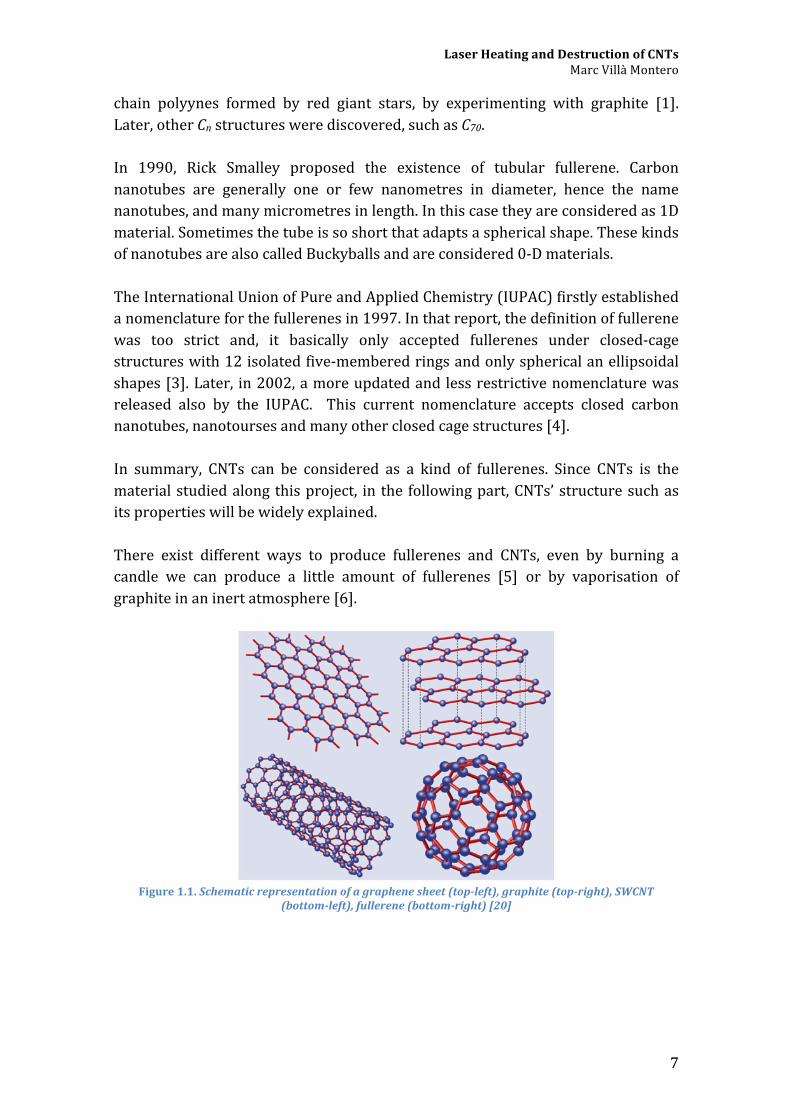
49
In the case where everything went as expected, eight laser-‐heating experiments should had been carried out, which not only involves the eight tests, but also preparation of the tests, previous trial tests, treating the data, analyse it and come up to some conclusions. The characterisation was finished four weeks before the final presentation of the report. By then, it was impossible to prepare and run the experiments expected so a new experimental plan was designed. The plan was to use a hermetic cell in order to reproduce a 100% argon atmosphere. The cell was hand-‐manufactured in Nancy, so it was not a very sophisticated device. The initial plan was to carry the experiments under air or argon flow rate using the input (red) and the output (blue) of the cell while the input was connected to the argon or air bottle and the output under water. Then the sample was supposed to be placed in the cell and then, through the glass, overheated by the laser.
Figure 5.1. Left side, picture from the argon gas-‐loading system with argon tank and its inputs and
outputs. Right side, picture from the cell manufactured in Nancy
Due to some manipulation unexpected pressure it was not possible to use the cell and the Linkam cell was used instead, as it will be explained in the final planning point. Firstly it was wanted to heat the samples applying a cyclic thermal load by means of the laser, as it was done in Maxime Noël master thesis [11], as displayed in figure 5.2.

Laser Heating and Destruction of CNTs Marc Villà Montero
50
Figure 5.2. Schema of the cyclic loading of high power density to CNTs [11]
This one was a very long test. It was expected to observe an intensity increase on the RBM profile due to desorption of the nanotubes followed by a decreasing of the signal due to overheating and destruction. After the characterisation of the material, it was decided to reschedule this tests making them shorter, focusing mainly on the study of the desorption process of impurities and external nanoparticles on the HiPCO tubes which was initially observed during the first 30 minutes of overheating.
5.2.2. Final planning The final planning differed a lot from the initial one. The main problem was the time. The bad work planning from one side and the optimistic original experimental plan lead to have not as much as time from the test as it was expected from the beginning. The green laser tests were deleted from the schedule, so the laser heating experiments were then focused on red laser tests. The experiments under the two different atmospheres were still up. It was still planned to test both type of CNTs but finally only the closed tubes were tested. To sum up, the final planning only involved laser heating of closed HiPCO nanotubes under red laser under argon and air atmosphere respectively. Due to differences between the tests under argon and air, only the results from argon atmosphere were considered.

Laser Heating and Destruction of CNTs Marc Villà Montero
51
Since the old hermetic cell broke during its manipulation, it was replaced for another cell obtained for the chemistry department at LTU. This cell was a very performance cell from Linkam Scientific Instruments®. This cell was easier to manipulate than the other one, so the set-‐up of the experiment was faster. The Linkam cell could also be used as a temperature chamber to study the thermal resistivity of the nanotubes using a low laser power.
5.3. Experimental method To understand the laser heating effect on the nanotubes, the sample was carefully placed on the cell stage. It was wanted to block the cell on the stage in order to avoid it to move. Unfortunately, the stage did not have anything to block it, so it was placed on the surface. It was important not to move the cell too much because of the risk of moving the sample from the spot. Once the sample was placed, the cell was correctly shut and sealed. Then, from one of its inputs, a tube connected to the gas-‐loading system was plugged. A die was placed in the output in order to allow the air remaining in the cell to scape. Then an argon flow was kept during some minutes in order to clean the inside of the cell from oxygen particles. Once it was considered that the only gas remaining in the cell was argon, the output was block by tacking off the die that was placed previously. Only few seconds after blocking the output, the tube from the argon bottle was unplugged. Thus, the gas remaining in the cell was 100% argon no pressure higher than atmosphere was introduced, so the experiment was ready to be run. Carefully the Linkam cell was placed on the stage in order to start the laser-‐heating test using the Raman spectroscope. The objective used in the microscope was a 50x objective with aperture of 0.95. Some defocusing problems were observed later on due to such a high precision of the objective. The heating method was similar to the one used in previous studies [11]. A first spectrum was taken at reference conditions, before starting the irradiation. After each heating step, the sample was brought back to room temperature in order to observe the irreversible heating effect caused on the nanotubes. In any case, spectra were collected during the heating process, even though it was difficult to observe the heating effects at that stage.

Laser Heating and Destruction of CNTs Marc Villà Montero
52
Firstly, the sample was heated up until 188°C during 15 minutes two times consecutively. Between each time, a 20 minutes spectrum at room temperature was collected. Afterwards, the laser power was increase, so the temperature increased with it until 288°C. Two heating steps were carried out at this temperature as well and, also, a spectrum at reference conditions was taken between them. In figure 5.3 a schematic representation of the method can be observed.
Figure 5.3. Thermal loading used in the laser heating tests in the Linkam cell under argon atmosphere
In the following points the reasons of the choice of these temperatures as well as how the temperature was controlled and calculated are largely explained. Several calibrations were done before starting the experiments. All them were mainly based on previous studies and methods. The possible influence of the glass of the cell between the objective and the sample was also studied. Previously to the final experiment, less specific tests were carried out in order to get a better understanding of the expected results and the test procedure. These first tests were carried out under both, argon and air, atmospheres but applying a random heating method. Therefore, the interpretation of the results is not evident and does not give a lot strong statements but rather interesting observations and help calibration. Thus, these results will be explained in the results parts as well.

Laser Heating and Destruction of CNTs Marc Villà Montero
53
5.4. Previous results The objective of the tests was to study the laser heating process on the nanotubes and during this process it was expected to observe desorption on the nanotubes. It was expected to observe evidences of annealing in the nanotubes and on their surfaces by studying the RBM profile. It is known that intensity of the RBM signal decreases when the nanotubes are being destroyed or overheated. But in precedent studies [11], it was also observed that during the very beginning of the overheating process, the RBM peaks experienced an increase of intensity for some minutes and, after reaching a maximum intensity, their intensity started to decrease due to overheating and degradation.
Figure 5.4. Desorption process observed in older studies [11]
The way to know if the intensity was increasing was to take the intensity value comprised between the baseline of the spectra and the studied peak. It was suspected that the increase of the signal during the beginning of the overheating was due to annealing of impurities and external nanoparticles foreign from the carbon nanotubes. In the case of empty nanotubes, desorption was expected to be less present, but still, than in the water-‐filled ones. Even though they are empty tubes, it is impossible to have 100% clean samples under the work conditions carried during the sample preparation and the sample storage. It is not difficult that some particles in the air got stuck to the sample. The aim was to find the intensity (temperature) where the foreign particles desorption took place but not the destruction of the nanotubes. So the main
a)
b)
c)
d)

Laser Heating and Destruction of CNTs Marc Villà Montero
54
objective was to find a constant intensity at what we can burn the impurities but not damage the tubes. The experiments were carried in sequences, starting with low power density and increasing in different steps. At some point, if there was existence of foreign particles, it was expected to observe an increase on the RBM intensity. The particles make the intensity drop because they can interfere on the vibration mode of the molecules. When they are destructed, the vibration mode of the molecules increases so the RBM intensity does as well. Depending on the way the nanotubes are contaminated a different evolution on the RBM intensity is expected. Three different scenarios were thought:
1) Case of super clean and pure tubes. The intensity drops with time due to lack of desorption and the only presence of overheating.
2) Case of impurities on the tubes surface. The intensity experiences an increase due to annealing of the particles on the surface. It can happen the other way around, but it would be unexpected.
3) Case of impurities on the surface and inside the tubes. That is the case expected for the water-‐filled open tubes. In this case it is expected to observe two clearly different steps. The first one is common to case 2, where the impurities are on the CNT surface; so first it should be observed an increase of the RBM intensity due to the destruction of the impurities on the surface. Following that, desorption in the internal particles of the CNT will take place, making the RBM intensity to increase again.
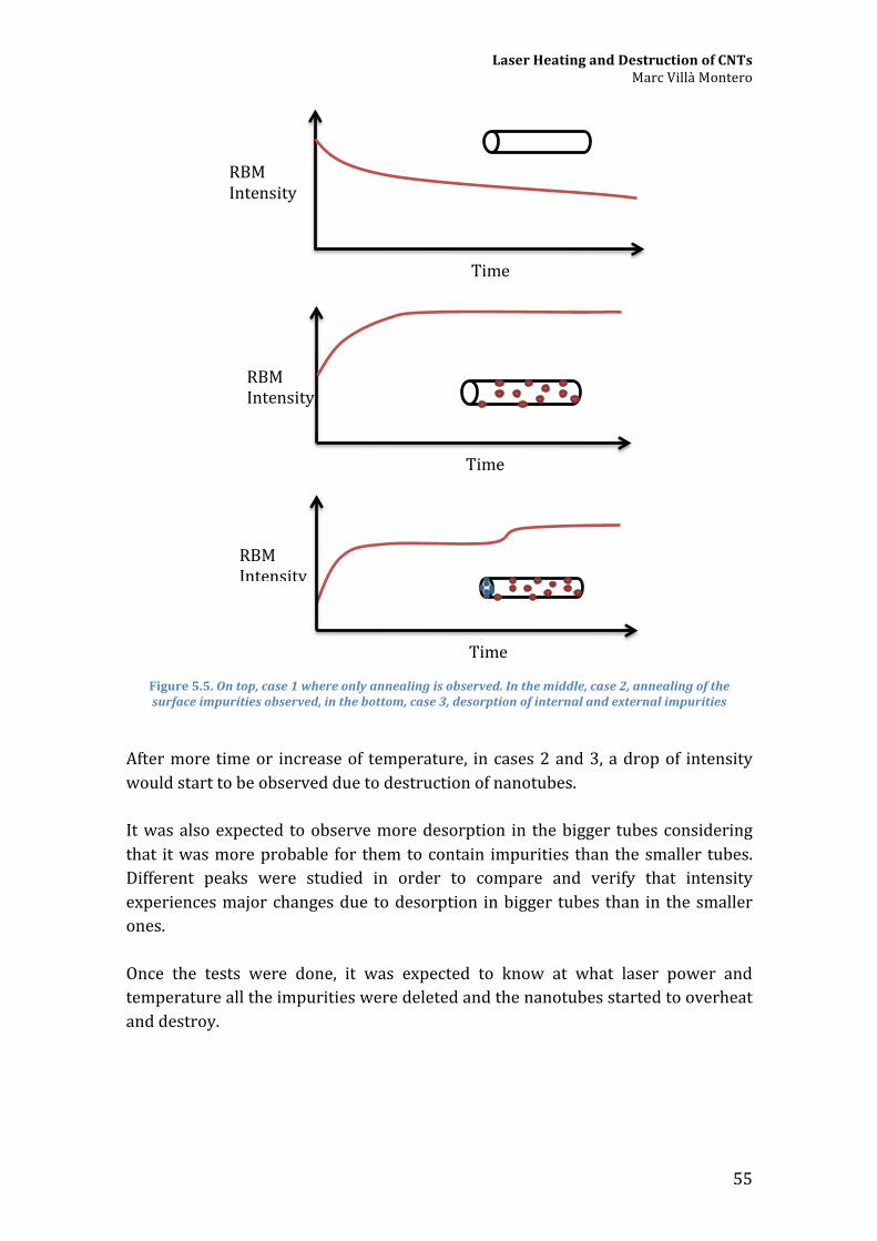
Laser Heating and Destruction of CNTs Marc Villà Montero
55
Figure 5.5. On top, case 1 where only annealing is observed. In the middle, case 2, annealing of the surface impurities observed, in the bottom, case 3, desorption of internal and external impurities
After more time or increase of temperature, in cases 2 and 3, a drop of intensity would start to be observed due to destruction of nanotubes. It was also expected to observe more desorption in the bigger tubes considering that it was more probable for them to contain impurities than the smaller tubes. Different peaks were studied in order to compare and verify that intensity experiences major changes due to desorption in bigger tubes than in the smaller ones. Once the tests were done, it was expected to know at what laser power and temperature all the impurities were deleted and the nanotubes started to overheat and destroy.
RBM Intensity
Time
RBM Intensity
Time
RBM Intensity
Time

Laser Heating and Destruction of CNTs Marc Villà Montero
56
5.5. Preliminary work Besides the characterisation, other measurements and preparations were needed in order to be able to start with the experiments. More samples were needed to be prepared and some calibrations were done in order to have as many laser parameters under control.
5.5.1. Sample and material preparation All material was cleaned using ethanol before running any experiment. The cell was cleaned carefully avoiding any scratch using a towel for microscope objectives. Regarding the sample preparation, the process followed was exactly the same as for the characterisation because the samples were exactly the same.
5.5.2. Calibrations
Several calibrations need to be done before any accurate experiment is run, and laser-‐heating experiments are not an exception. In our case, it is important to know the relation between the power output of laser and the temperature in the sample. Moreover, because we cannot move the sample in order to keep the same spot of observation, we have to make sure we control this power output (by calibrating micrometer screw on laser-‐head) and also know what power is actually reaching the stage and finally in the cell, on the sample.
5.5.2.1. Temperature – Laser power
Before carrying out the final tests, a characterisation relating the laser power in the fiber the temperature was done. It was done by studying the shift of the G-‐band peak and relating it with the relation of 0.025 cm-‐1/K [26]. This calibration was basic in order to know at what exact temperature the nanotubes were experiencing annealing process or were being destroyed. The principle was simple. By always studying exactly the same sport, a first spectrum of the G-‐band was taken at low power (reference power or less). On that power, the nanotubes are not degraded neither overheated so the temperature considered then is the room temperature (20°C).

Laser Heating and Destruction of CNTs Marc Villà Montero
57
Then the laser power was increased smoothly and for each power increase, the power was measured in the fiber. It was not possible to measure the laser power on stage due to the fact that the calibration needed to be done always at the same spot. By increasing the laser power, the G-‐band experienced a shift to lower frequency (figure 5.6). This shift was characterised, as mentioned before, as 0.025 cm-‐1/K.
Figure 5.6. Evolution of the G-‐band of Closed HiPCO tubes under air conditions and red laser under
different laser powers
As shown on table 5.1, it was possible to calculate an approximate radiation temperature. It is important to mention that the laser power in the fiber was not the same as the power obtained on stage. Between the stage and the fiber, there was observed a big loss of power, even bigger than the one observed in previous studies. In the microscope it is usual to have a loss of power due to ageing of the materials, dirtiness and other factors. Also this power loss has a big dependence on the objective used. For the laser-‐heating experiments, the objective used was a 50x. It was known that by using the 20x objective, the loss between the fiber and the stage was about a 44%. For the 50x objective, some tests were done in order to find out the efficiency. The power-‐loss measured was of 88%, which is way too much than expected. Laser Power in fiber
(mW) Lase power on stage (mW)
G-‐band shift (cm-‐1)
Temperature (°C)
1.15 0.25 1592.5 20 2.11 0.46 0.8±0.05 50-‐52 4.25 0.935 1.9±0.1 96-‐100 6 1.32 3.3±0.2 144-‐152 8.2 1.804 4.8±0.3 212-‐220
Table 5.1. Data obtained during the calibration that relates laser power with temperature

Laser Heating and Destruction of CNTs Marc Villà Montero
58
Once the temperature was known it was possible to control the temperature induced to the tubes by knowing the laser-‐power applied. The behaviour was quite lineal, as it can be observed in figure 5.7.
Figure 5.7. Linear relation between laser power and temperature on stage under Air atmosphere using
Red Laser
5.5.2.2. Micrometre position – Laser power More calibrations were needed to know the exact laser power applied. The laser power was regulated by means of a micrometre placed on the laser output to the fiber. By screwing the micrometre it was possible to allow the laser go through the fiber. After running some tests, it was observed that it was very difficult to set an exact laser power for the studies. That was making the studies more random and complicating the results analysis. It was decided, then, to find a relationship between the opening of the micrometre and the laser power supplied on stage in order to be able to set a suitable temperature/laser power for the studies. One first thought was that the opening in micrometres should have a linear relationship with the laser-‐power on stage. After analysing the data, it was found out that the behaviour was not linear at all, which has its explanation. When opening a light beam, it increases in all radial directions, so the intensity first increases exponentially, until it reaches a maximum when it smoothly stabilises.
y = 123,23x -‐ 10,94 R² = 0,99579
0
50
100
150
200
250
0 0,2 0,4 0,6 0,8 1 1,2 1,4 1,6 1,8 2
Temperature (°C)
Laser Power on stage (mW)
Temperature vs Laser power on stage

Laser Heating and Destruction of CNTs Marc Villà Montero
59
Figure 5.8. Relation between the micrometre position of the Red Laser and the laser power measured
on stage fitted with a 3rd order polynomial and using a 50x (0.95) objective
The approximate 3rd order polynomial had a quite high coefficient of determination (R2) of 0.991. Even though it is not a perfect fit, it can be used to predict the laser power on stage when using a 50x (0.95) objective for a determinate micrometre position. This plot or the same calibration method can be used in coming studies to control the laser power and the temperatures applied on the nanotubes.
5.5.2.3. Glass of the cell – Laser power Since some tests were run using the Linkam cell, it was decided to study the influence of the glass of this cell on the laser power. Glass produces always some reflection and this reflection influences the amount of light that can go through the material and, therefore, on the laser power obtained inside the cell.
Figure 5.9. Representative picture showing the method used to calculate the laser power under the glass

Laser Heating and Destruction of CNTs Marc Villà Montero
60
There was the possibility that the influence of the glass was devastating, reducing dramatically the laser power inside the cell. To test so, it was measured first the laser power on stage and then the glass was placed on the powermeter. It was tried to reproduce exactly the same distances it would have during the tests. As showed in figure 5.10, it was observed that the glass did not affect very much to the laser beam and the 95.68% of it was able to go through.
Figure 5.10. Relation between the laser power on stage and the laser power under the glass of the
Linkam cell
It could be considered that the glass has a minimal effect on the laser power. It is very possible that the glass was previously treated in order to have less refraction and reflection.
5.6. Results
5.6.1. First results First experiments were run before the final one in order to understand the future results and prevent possible issues during the final experiment. These first training tests were done under red laser since it was already known that there would not be enough time to carry out the experiments under green laser. The cell was first loaded with argon gas as it was done for the final test. In the first case, the heating process was not controlled as precisely as it was done later on. Differently from the final test, any spectrum was taken under reference conditions. The evolution of the intensity was calculated directly from the display of WiTec
y = 0,9568x R² = 0,99947
0 0,5 1
1,5 2
2,5 3
3,5 4
0 1 2 3 4 5
Laser Power under glass (real)
(mW)
Laser Power without the glass (mW)
Calibration of the laser power under the cell

Laser Heating and Destruction of CNTs Marc Villà Montero
61
software since it was considered precisely enough to give an overall idea about the heating effect. In figure 5.11, the method to observe the evolution of intensity is represented. A reference line from the whole spectrum was taken into account and compared with the high of each peak. Firstly, the highest peak was used due to the fact that it was easier to observe possible changes in the most intense peaks. Later on, the peaks corresponding to bigger tubes were used since it was expected to observe a bigger desorption in bigger tubes.
Figure 5.11. Method used to observe in a fast way the increase of intensity on WiTec system
As expected, an increasing evolution of the RBM intensity was observed in argon and air atmospheres, without treating extensively the data. As can be observed in figure 5.12 and 5.13, the temperature was increased by the laser power and first an increase of the intensity of the RBM was observed. After a certain time and temperature, the intensity stopped to increase and started to decrease. The two steps, desorption and destruction, were successfully observed. Nevertheless, the fact that the temperature was not increased using normalised steps, made the results very difficult to analyse. For the test under argon atmosphere (figure 5.12), while increasing the temperature, it was observed an increase of the intensity from the baseline until reaching a temperature of 476°C. Afterwards, the intensity started to decrease. Clearly, desorption of particles in the nanotubes occurred and then it was followed by destruction of them. It is very difficult to guarantee that the temperature at what desorption ends is 476°C. Previously, the sample was submitted to irradiation during a long period of time at 138°C. CNTs do not show destruction at that temperature but the factor of heating resistance can have an important role in

Laser Heating and Destruction of CNTs Marc Villà Montero
62
this aspect. The presence of too many factors that may influence the behaviour of tubes under heating males these results hard to interpret. To conclude with the argon atmosphere test, it could be said that under argon the temperature of destruction was quite high, over 400°C. It was expected to observe a good resistance to destruction due to lack of oxygen molecules in the atmosphere. Comparing the results with the test run under oxygen atmosphere, this though was restated.
Figure 5.12. Evolution of the intensity of peak n°6 (255cm-‐1) with time related with the temperature
(discontinuous line) for SWCNTs under argon atmosphere
The same kind of test was carried out under air atmosphere, without adding any gas. Then, it was expected to observe a faster destruction of the nanotubes. Unfortunately, the heating process was not controlled as wanted due to the fact that every bundle is different and react differently to the same power input, making the calibration for temperature more indicative than definitive. So, as it happened with the test explained before, it was difficult to come up to very strong conclusions with the results obtained from this test. As shown in figure 5.13, desorption and destruction was observed as it was for the test under argon. The main difference was the temperature. Destruction occurred at a much lower temperature than in the previous case due to the presence of oxygen molecules in the cell. Oxygen molecules make the CNTs oxidise much faster due to burning. Destruction was observed at 216°C and it also appeared sooner than in the other case. In this case, a long step at HPD was not taken.

Laser Heating and Destruction of CNTs Marc Villà Montero
63
Figure 5.13. Evolution of the intensity of peak n°6 (255cm-‐1) with time related with the temperature
(discontinuous line) for SWCNTs under air atmosphere (O2)
Since it was expected to observe a bigger change of intensity in the bigger tubes, the evolution of the intensity in different peaks was analysed. It was expected to observe a clear difference between bigger tubes (metallic) and smaller tubes (semiconducting). Since bigger tubes can adsorb more molecules and particles, it was expected to observe more evidences of desorption on them. In figure 5.14, it can be observed the evolution of peak 2 (192 cm-‐1) and peak 6 (255 cm-‐1) with the time while being heated. It seems that the bigger tubes show a faster desorption than the smaller tubes, as it can be observed after the first increase of temperature, as expected. Nevertheless, the results are not very clear and evident because afterwards, the bigger tubes seem to be destroyed faster than the smaller ones.
Figure 5.14. Comparison the evolution of the intensity during heating

Laser Heating and Destruction of CNTs Marc Villà Montero
64
The aim of this first tests was not to come up with definitive statements and conclusions, but to have a first idea about the parameters to use during the final test.
5.6.2. Final results As described before, the final test was done while taking into account the first trial tests done and the previous published works. The first tests were useful in order to know what steps and temperatures set. An interesting information obtained from these test was the temperature at what to work and expect to observe desorption. As mentioned before, the heating tests were planned to be done ant 188°C and 288°C. From these previous tests, it was observed that at 170°C destruction did not start to occur (figure 5.15). So the tests were started from a similar temperature as this one. A liner behaviour was observed during desorption while observing the evolution of intensity as function of the temperature, then it was possible to predict the temperature at what the desorption would stop: 288°C.
Figure 5.15. Evolution of the intensity depending on the temperature during the first heating tests under
argon atmosphere in the Linkam cell. Linear behaviour observed
After the four heating steps at HPD, the spectra collected at LPD were the ones showed in figure 5.16. Regarding all peaks, a clear evolution was observed after treating the data and PeakFitting the spectra. It was observed that the tubes on the higher frequencies did not show evidences of desorption, just the opposite, they decreased intensity after reaching 288°C, so they were burned. On the other hand,

Laser Heating and Destruction of CNTs Marc Villà Montero
65
the tubes observed in the lower frequencies showed desorption from the very beginning by increasing intensity. Also, the bigger tubes, observed in the lower intensity, they did not show destruction at any time, not even at 288°C.
Figure 5.16. Evolution of the RBM profile after heating the SWCNTs under argon atmosphere
For a better understanding of the figure, one should indicate that when the lase-‐power in fiber was set to 3mW, the temperature on stage was about 188°C, while when the laser power was 5mW the temperature was 288°C. The spectra were taken at the same conditions, at LPD after each heating step. All spectra obtained during the test were compared to a reference one (figure 5.17), taken at the same spot before starting the heating test at reference conditions with low power density (LPD). Peakfitting analysis was done equally for all RBM spectra in order to be able to study the evolution of all peaks.

Laser Heating and Destruction of CNTs Marc Villà Montero
66
Figure 5.17. Reference RBM spectrum at LPD under argon atmosphere using red laser
5.7. Conclusion To conclude it can be said that desorption was observed from 188°C in the bigger tubes, the first heating step and it was still present at 288°C. It is unknown if desorption is observed also at lower temperature. To find out so, it would be interesting to run experiments at lower temperature. It was observed that bigger desorption was observed in the bigger tubes. That can be due to its size, which makes them more likely to contain impurities and also foreign particles and molecules are more likely to get attached on them. Also it is know that bigger tubes (with peak position less than 255cm-‐1 in the RBM spectra) that are well known for their metallic properties, they are more likely to absorb particles and molecules and, therefore, they are more likely to desorb them. Then, this particles act like a shield on the big tubes. As soon as they get destroyed, the spectroscope collects information directly from the tubes, what can explain the increase of intensity. On the other hand, it was observed that smaller tubes (observed at higher frequency than 255cm-‐1) they did not show desorption, at least not big evidences. At 188°C the intensity of the RBM peak at 282cm-‐1 was not affected, but after increasing the temperature up to 288°C, the intensity dropped showing destruction and overheating. What can explain the increase of intensity for big tubes while small tubes are being destructed is that, small tubes can act on the big tubes, as they were impurities, so the impurities that are being destroyed at the beginning are just the smallest tubes. Of course, it is just a hypothesis, but it would be interesting to perform further
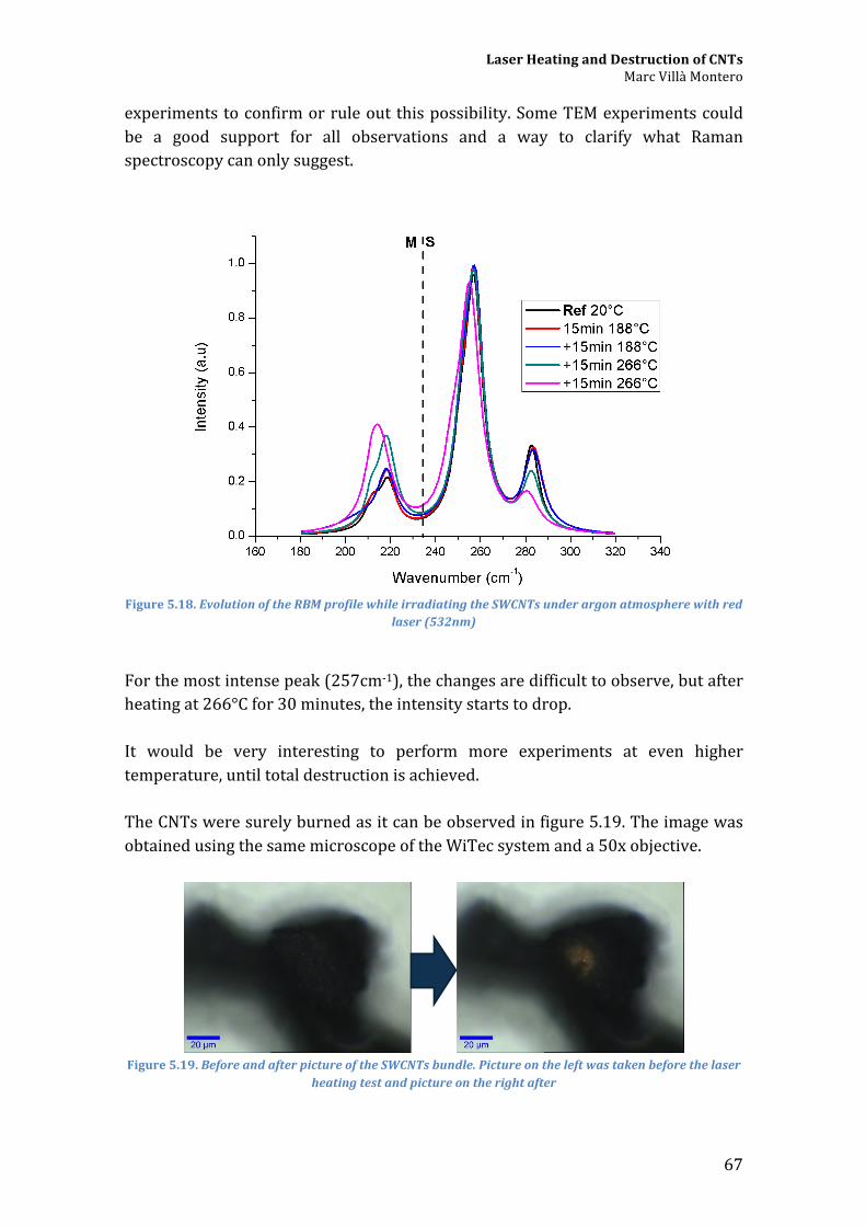
Laser Heating and Destruction of CNTs Marc Villà Montero
67
experiments to confirm or rule out this possibility. Some TEM experiments could be a good support for all observations and a way to clarify what Raman spectroscopy can only suggest.
Figure 5.18. Evolution of the RBM profile while irradiating the SWCNTs under argon atmosphere with red
laser (532nm)
For the most intense peak (257cm-‐1), the changes are difficult to observe, but after heating at 266°C for 30 minutes, the intensity starts to drop. It would be very interesting to perform more experiments at even higher temperature, until total destruction is achieved. The CNTs were surely burned as it can be observed in figure 5.19. The image was obtained using the same microscope of the WiTec system and a 50x objective.
Figure 5.19. Before and after picture of the SWCNTs bundle. Picture on the left was taken before the laser
heating test and picture on the right after
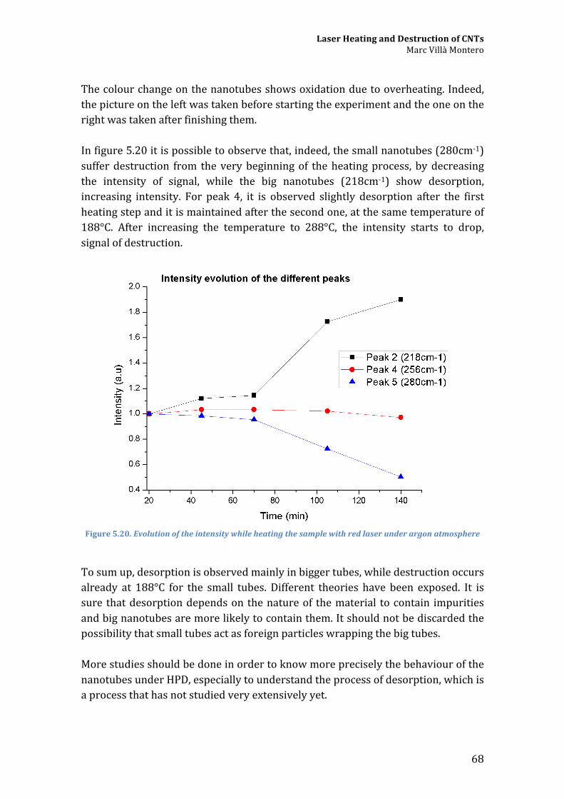
Laser Heating and Destruction of CNTs Marc Villà Montero
68
The colour change on the nanotubes shows oxidation due to overheating. Indeed, the picture on the left was taken before starting the experiment and the one on the right was taken after finishing them. In figure 5.20 it is possible to observe that, indeed, the small nanotubes (280cm-‐1) suffer destruction from the very beginning of the heating process, by decreasing the intensity of signal, while the big nanotubes (218cm-‐1) show desorption, increasing intensity. For peak 4, it is observed slightly desorption after the first heating step and it is maintained after the second one, at the same temperature of 188°C. After increasing the temperature to 288°C, the intensity starts to drop, signal of destruction.
Figure 5.20. Evolution of the intensity while heating the sample with red laser under argon atmosphere
To sum up, desorption is observed mainly in bigger tubes, while destruction occurs already at 188°C for the small tubes. Different theories have been exposed. It is sure that desorption depends on the nature of the material to contain impurities and big nanotubes are more likely to contain them. It should not be discarded the possibility that small tubes act as foreign particles wrapping the big tubes. More studies should be done in order to know more precisely the behaviour of the nanotubes under HPD, especially to understand the process of desorption, which is a process that has not studied very extensively yet.

Laser Heating and Destruction of CNTs Marc Villà Montero
69
5.8. Future studies The time planning of this project was not successfully completed due to lack of time. Also, the characterisation part took longer than expected and some time that was kept for the testing part, was used in the characterisation instead. So the principal studies that can be carried out in the department are:
-‐ Same laser heating process using open SWCNTs instead of closed ones under argon atmosphere
-‐ Same laser heating process using closed SWCNTs under air atmosphere -‐ Same laser heating process using open SWCNTs under air atmosphere -‐ All these tests using a different laser, green laser for example (633nm) since
it is the one available in the lab It would be interesting to reproduce the same heating process but using smaller temperature steps, increase the temperature more slowly. Then it would be expected to observe all the steps of desorption. The test would be much longer then. It would be expected to observe faster destruction and desorption in open SWCNTs (water-‐filled) and also, by using the green laser, it would be possible to observe smaller tubes that would be destroyed faster. Tests under air, due to the presence of oxygen molecules, would show faster destruction of the nanotubes, as explained before. The tests already done could be re-‐done by using another objective, 20x instead of 50x. It has been observed some problems due to focusing using the 50x objective after heating the sample. By using the 20x objective this change of focus would have little influence on quality of spectra. Finally some heating resistance test could be carried out using the Linkam cell. The cell used before was much more difficult to manipulate than the new one. Some tests using LPD and increasing the temperature of the cell, by using its software, could be interesting to do in order to observe effects due to only heating by avoiding irradiance.
Laser Heating and Destruction of CNTs Marc Villà Montero
70
References [1] Carbon Nanotubes Properties and Applications, Taylor and Francis, Edited by Michael J. O’Connell, 0-‐8493-‐2748-‐2 [2] http://www.chemguide.co.uk/atoms/structures/giantcov.html 18/09/2013, 15:57 [3] Godly, E. W. and Taylor, R. Nomenclature and Terminology of Fullerenes: A Preliminary Survey, Pure and Applied Chemistry, vol. 69(7), 1411-‐1434 (1997) [4] W. H. Powell et al. Nomenclature for C60-‐Ih and C70-‐D5h8(6) fullerenes, Pure and Applied Chemistry, Vol. 74, No. 4, pp. 629-‐695, 2002 [5] Li, Y and Hsieh, C. Synthesis of carbon nanotubes by combustion of a paraffin wax candle, September 2007, Micro & Nano Letters, IET, Vol. 2, pp. 63-‐66. 1750-‐0443 [6] Lowell D. Lamb and Donald R. Huffman, Fullerene Production, June 1993, J. Phys. Chem. Solids Vol. 54, No. 12, pp. 1635-‐1643 [7] S. Handuja, S. Preet Singh, P. Srivastava, V.D. Vankar, Growth of long aligned CNTs on amorphous hydrogenated silicon nitride by thermal chemical vapour disposition, 2009, Materials Letters, Vol. 63, pp. 1249-‐1251 [8] M.S. Dresselhaus, G. Dresselhaus, R. Saito, A. Joiro, Raman Spectroscopy of carbon nanotubes, 2005, Physics Reports, vol. 409, pp. 47-‐99 [9] W. Evans, L. Hu, P. Keblinski, Thermal conductivity of graphene ribbons from equilibrium molecular dynamics: Effect of ribbon width, edge roughness, and hydrogen termination, 2010, Applied Physics Letters, vol. 96, pp. 203112 [10] Alexander A. Balandin, Thermal properties of graphene and nanostructured materials, August 2011, Nature Materials, Vol. 10, pp. 569-‐581 [11] M. Noël, Raman Characterisation and laser heating effects in carbon nanotubes, Master Thesis, Luleå University of Technology [12] S. Reich, C. Thomsen, J. Maultzsch, Carbon Nanotubes: basic concepts and physical properties, 2004, Wiley-‐VCH Verlag GmbH & Co. KGaA, ISBN: 3-‐527-‐40386-‐8 [13] G. Hummer, J. Rasaiah, J. Noworyta, Water conduction through the hydrophobic channel of a carbon nanotube, Nature, 2001, vol. 414, pp. 188-‐199 [14] S. Cambré, B. Schoeters, S. Luyckx, E. Goovaerts and W. Wenseleers, Experimental observation of single-‐file water filling of thin single-‐wall carbon nanotubes down to chiral index (5,3), Physical Review Letters, 2010, vol. 104, pp. 207401 [15] M. Longhurst, N. Quirke, The environmental effect on the radial breathing mode of carbon nanotubes. II. Shell model approximation for internally and externally absorbed fluids, The Journal of chemical physics, 2006, vol. 125, pp. 184705 [16] S. Cambré, S. Santos, W. Wenseleers et al. Luminescence properties of individual and water-‐filled single-‐walled carbon nanotubes, ACS Nano, 2012, Vol. 6, pp. 2649-‐2655

Laser Heating and Destruction of CNTs Marc Villà Montero
71
[17] T. Belin, F. Epron, Characterisation methods of carbon nanotubes: a review, Materials Science and Engineering B, 2005, vol. 119, pp. 105-‐118 [18] E. Smith, G. Dent, Modern Raman Spectroscopy, a practical approach, 1989, Springer-‐Verlag, ISBN: 0-‐471-‐49668-‐5 [19] http://www.raman.de/htmlEN/basics/intensityEng.html, 29/09/2013, 16:03] [20] A. H. Castro Neto, F. Guinea, N. M. R. Peres, Drawing conclusions from graphene, Physics World, 2006, vol. 19, pp. 33 [21] H. Kataura, Y. Kumezawa et al. Optical properties of Single-‐walled Carbon Nanotubes, Synthetic metals, 1999, vol. 103, pp. 2555-‐2558 [22] J. Salvetat, J. Bonrad, N. Thomson et al. Mechanical Properties of carbon nanotubes, Applied Phyiscs A: Material Science and Processing, 1999, vol. 69, pp. 255-‐260 [23] M. Scarselli et al. Electronic and optoelectronic nano-‐devices based on carbon nanotubes [24] http://ykkato.t.u-‐tokyo.ac.jp/nanotubechirality.en.html, 20/09/2013, 11:05 [25] http://www.teachers.yale.edu/curriculum/viewer/, 19/09/2013, 9:34 [26] Y. Zhang, L. Xie, J. Zhang et al. Temperature coefficients of Raman frequency of individual Single-‐Walled Carbon Nanotubes, The Journal of Physical Chemistry letters, 2007, Vol. 111, pp. 14031-‐14034 [27] http://www.bruker.com/, 27/12/2013, 14:05 [28] T. Dieing, O. Hollricher, J. Toporski, Confocal Raman Microscopy, Springer Series in Optical Sciences, 2011, vol. 158 [29] http://www.originlab.com/, 27/12/2013, 14:45 [30] http://www.sigmaplot.com/products/peakfit/peakfit.php, 27/12/2013, 15:00

Laser Heating and Destruction of CNTs Marc Villà Montero
72
Table of figures Figure 1.1. Schematic representation of a graphene sheet (top-‐left), graphite (top-‐
right), SWCNT (bottom-‐left), fullerene (bottom-‐right) [20] ......................................... 7 Figure 1.2. Schematic representation of Ch vector and the basis vectors of graphite
[24] ...................................................................................................................................................... 8 Figure 1.3. In green, Ch vector, in red, armchair section and in bold black zig-‐zag
structure [23] ................................................................................................................................... 9 Figure 1.4. Structure of each class of CNT [25] ............................................................................ 9 Figure 1.5. Modulus vs. Disorder in MWCNTs [22] .................................................................. 13 Figure 2.1. Interaction between a photon and matter characterised by energy states
............................................................................................................................................................ 15 Figure 2.2. Spectrum example showing the different scatterings as a function of the
wavenumber and wavelength [19] ....................................................................................... 16 Figure 2.3. Raman spectrum showing the principal characteristics of CNTs. Spectrum
obtained from and individualised SWCNTs with diameter about 1.07nm, using a E=1.16 eV laser [17] ................................................................................................................... 17
Figure 2.4. Kataura plot for SWCNTs for 𝛾=2.75 𝑒𝑉. Solid circles indicates metallic SWCNTs and the empty ones, semiconducting SWCNTs. The arrows show the diameter distributions of each catalyst [21] .................................................................... 18
Figure 2.5. Evolution of the G-‐band position as function of the temperature [26] ..... 19 Figure 4.1. Influence of water filling of SWCNTs in the RBM spectra, Red (grey)
belongs to closed (empty) tubes and blue (dark grey) corresponds to open (water-‐filled tubes) [14] ........................................................................................................... 24
Figure 4.2. Bad quality RBM spectra due to bad settings. At the left side, RBM spectrum from Open HiPCO using 5s integration time and 12 accumulations. At the right side, RBM spectrum from Closed HiPCO using 3s integration time and 10 accumulations ........................................................................................................................ 27
Figure 4.3. Spectra collection corresponding to the Red laser characterisation of Closed HiPCO nanotubes ........................................................................................................... 28
Figure 4.4. Characteristic peaks observed under red laser .................................................. 29 Figure 4.5. Plot representing the peak position of each characteristic peak and its
error in the closed HiPCO tubes under Red Laser ....................................................... 30 Figure 4.6. Spectra collection corresponding to the Red laser characterisation of
Open HiPCO nanotubes ............................................................................................................. 31 Figure 4.7. Plot representing the peak position of each characteristic peak and its
error in the Open HiPCO tubes under Red Laser ............................................................. 33 Figure 4.8. Spectra collection corresponding to the Green laser characterisation of
Closed HiPCO nanotubes ........................................................................................................... 34 Figure 4.9. Comparison of a random RBM spectra obtained in each different closed
HiPCO aggregate studied with Green Laser ..................................................................... 35 Figure 4.10. Aggregates 1, 2 and 3 and 4 .................................................................................... 35 Figure 4.11. Characteristic peaks observed under green laser ........................................... 36 Figure 4.12. Plot representing the peak position of each characteristic peak and its
error in the closed HiPCO tubes under Green Laser ....................................................... 37 Figure 4.13. Spectra collection corresponding to the Green laser characterisation of
Open HiPCO nanotubes ............................................................................................................. 38 Figure 4.14. Plot representing the peak position of each characteristic peak and its
error in the open HiPCO tubes under Green Laser ......................................................... 40

Laser Heating and Destruction of CNTs Marc Villà Montero
73
Figure 4.15. Width comparison of the characteristic peaks between open and closed tubes under Red Laser ............................................................................................................... 41
Figure 4.16. Width comparison of the characteristic peaks between open and closed tubes under Green Laser ........................................................................................................... 42
Figure 4.17. Peak position comparison of the characteristic peaks between open and closed tubes under Red Laser ................................................................................................. 44
Figure 4.18. Overlapping of two spots from open and closed nanotubes under Red Laser ................................................................................................................................................. 45
Figure 4.19. Peak position comparison of the characteristic peaks between open and closed tubes under Green Laser ............................................................................................. 46
Figure 4.20. Overlapping of two spots from open and closed nanotubes under Green Laser ................................................................................................................................................. 46
Figure 5.1. Left side, picture from the argon gas-‐loading system with argon tank and its inputs and outputs. Right side, picture from the cell manufactured in Nancy ............................................................................................................................................................ 49
Figure 5.2. Schema of the cyclic loading of high power density to CNTs [11] ............... 50 Figure 5.3. Thermal loading used in the laser heating tests in the Linkam cell under
argon atmosphere ....................................................................................................................... 52 Figure 5.4. Desorption process observed in older studies [11] ............................................ 53 Figure 5.5. On top, case 1 where only annealing is observed. In the middle, case 2,
annealing of the surface impurities observed, in the bottom, case 3, desorption of internal and external impurities ........................................................................................... 55
Figure 5.6. Evolution of the G-‐band of Closed HiPCO tubes under air conditions and red laser under different laser powers ................................................................................ 57
Figure 5.7. Linear relation between laser power and temperature on stage under Air atmosphere using Red Laser ................................................................................................... 58
Figure 5.8. Relation between the micrometre position of the Red Laser and the laser power measured on stage fitted with a 3rd order polynomial and using a 50x (0.95) objective .................................................................................................................. 59
Figure 5.10. Relation between the laser power on stage and the laser power under the glass of the Linkam cell ..................................................................................................... 60
Figure 5.11. Method used to observe in a fast way the increase of intensity on WiTec system .............................................................................................................................................. 61
Figure 5.12. Evolution of the intensity of peak n°6 (255cm-‐1) with time related with the temperature (discontinuous line) for SWCNTs under argon atmosphere ..... 62
Figure 5.13. Evolution of the intensity of peak n°6 (255cm-‐1) with time related with the temperature (discontinuous line) for SWCNTs under air atmosphere (O2) . 63
Figure 5.14. Comparison the evolution of the intensity during heating .......................... 63 Figure 5.15. Evolution of the intensity depending on the temperature during the first
heating tests under argon atmosphere in the Linkam cell. Linear behaviour observed .......................................................................................................................................... 64
Figure 5.16. Evolution of the RBM profile after heating the SWCNTs under argon atmosphere .................................................................................................................................... 65
Figure 5.17. Reference RBM spectrum at LPD under argon atmosphere using red laser .................................................................................................................................................. 66
Figure 5.18. Evolution of the RBM profile while irradiating the SWCNTs under argon atmosphere with red laser (532nm) .................................................................................... 67
Figure 5.19. Before and after picture of the SWCNTs bundle. Picture on the left was taken before the laser heating test and picture on the right after .......................... 67

Laser Heating and Destruction of CNTs Marc Villà Montero
74
Tables Summary Table 1.1. Thermal conductivity of graphene and CNTs [10] .............................................. 12 Table 4.1. Observed peaks in the RBM from closed HiPCO tubes under Red Laser. Each
average was obtained by analysing all spots ................................................................... 29 Table 4.2. Observed peaks in the RBM from open HiPCO tubes under Red Laser. Each
average was obtained by analysing all spots ................................................................... 32 Table 4.3. Observed peaks in the RBM from closed HiPCO tubes under Green Laser.
Each average was obtained by analysing all spots ........................................................ 36 Table 4.4. Observed peaks in the RBM from open HiPCO tubes under Green Laser.
Each average was obtained by analysing all spots ........................................................ 39 Table 4.5. Study of the peak-‐width evolution in the case of Red Laser characterisation
............................................................................................................................................................ 41 Table 4.6. Study of the peak-‐width evolution in the case of Green Laser
characterisation .......................................................................................................................... 42 Table 4.7. Study of the peak-‐position in the case of Red Laser characterisation ......... 44 Table 4.8. Study of the peak-‐position in the case of Red Laser characterisation ......... 45 Table 4.9. Data compilation for the characterisation of HiPCO tubes under red and
green laser ..................................................................................................................................... 47 Table 5.1. Data obtained during the calibration that relates laser power with
temperature .................................................................................................................................. 57

Laser Heating and Destruction of CNTs Marc Villà Montero
75
Appendixes
1. Characterisation results without data treatment for green laser (532nm)
Appendix 1. Data obtained for characterisation of closed tubes using Green Laser (532nm)

Laser Heating and Destruction of CNTs Marc Villà Montero
76
Appendix 2. Data obtained for characterisation of open tubes using Green Laser (532nm)
2. Characterisation results without data treatment using red laser (633nm)
Appendix 3. Data obtained for characterisation of closed tubes using Red Laser (633nm)
200 240 280
0.3
0.6
0.9
Intens
ity
W avenumber (cm-‐1)
S pot 1 S pot 2 S pot 3 S pot 4 S pot 5
200 250 300
0.3
0.6
0.9
Intens
ity
W avenumber (cm-‐1)
S pot 1 S pot 2 S pot 3 S pot 4 S pot 5
200 250 300
0.3
0.6
0.9
Intens
ity
W avenumber (cm-‐1)
S pot 1 S pot 2 S pot 3

Laser Heating and Destruction of CNTs Marc Villà Montero
77
Appendix 4. Data obtained for characterisation of open tubes using Red Laser (633nm)
3. PeakFit process used to treat the data obtained from the spectroscope for
the characterisation and the results analysis from the heating test
Appendix 5. Example of the PeakFit analysis during characterisation using several peaks
200 250 300
0.3
0.6
0.9Spo
t 1
W avenumber (cm-‐1)
S pot 1 S pot 2
200 240 280
0.3
0.6
0.9
Spo
t 1
W avenumber (cm-‐1)
S pot 1 S pot 2 S pot 3 S pot 4
200 240 280
0.3
0.6
0.9
Intens
ity
W avenumber (cm-‐1)
S pot 1 S pot 2 S pot 3 S pot 4
200 240 280
0.3
0.6
0.9
Spo
t 1
W avenumber (cm-‐1)
S pot 1 S pot 2 S pot 4 S pot 5 S pot 6

Laser Heating and Destruction of CNTs Marc Villà Montero
78
Appendix 6. Example of the PeakFit analysis after the heating test using only 5 peaks


