

Phenomenological aspects Phenomenological aspects of magnetized brane models of magnetized brane models Tatsuo KobayashiTatsuo Kobayashi1.1. IntroductionIntroduction
2. Magnetized extra dimensions2. Magnetized extra dimensions3. N-point couplings and flavor symmetries3. N-point couplings and flavor symmetries44 .. Massive modesMassive modes5. Flavor and Higgs sector5. Flavor and Higgs sector6. Summary6. Summary based on collaborations with based on collaborations with H.Abe, T.Abe, K.S.Choi, Y.Fujimoto, Y.Hamada,R.Maruyama, T.Miura, H.Abe, T.Abe, K.S.Choi, Y.Fujimoto, Y.Hamada,R.Maruyama, T.Miura,
M.Murata, Y.Nakai, K.Nishiwaki, H.Ohki,M.Murata, Y.Nakai, K.Nishiwaki, H.Ohki, A.Oikawa, M.Sakai, M.Sakamoto, K.Sumita, Y.TatsutaA.Oikawa, M.Sakai, M.Sakamoto, K.Sumita, Y.Tatsuta

1 1 IntroductionIntroduction
Extra dimensional field theories, Extra dimensional field theories,
in particular in particular
string-derived extra dimensional field string-derived extra dimensional field theories, theories,
play important roles in particle physicsplay important roles in particle physics
as well as cosmology .as well as cosmology .

Extra dimensionsExtra dimensions 4 + n dimensions4 + n dimensions
4D ⇒4D ⇒ our 4D space-timeour 4D space-time
nD nD ⇒ ⇒ compact spacecompact space Examples of compact spaceExamples of compact space
torus, orbifold, CY, etc. torus, orbifold, CY, etc.

Field theory in higher Field theory in higher dimensionsdimensions
10D 10D ⇒ ⇒ 4D our space-time + 6D space4D our space-time + 6D space
10D vector10D vector
4D vector + 4D scalars 4D vector + 4D scalars
SO(10) spinor ⇒SO(10) spinor ⇒ SO(4) spinor SO(4) spinor
x SO(6) spinorx SO(6) spinor
internal quantum internal quantum number number
mM AAA ,

Several Fields in higher Several Fields in higher dimensionsdimensions 4D (Dirac) spinor4D (Dirac) spinor
⇒ ⇒ (4D) Clifford algebra (4D) Clifford algebra (4x4) gamma matrices (4x4) gamma matrices represention space ⇒ spinor representationrepresention space ⇒ spinor representation 6D Clifford algebra 6D Clifford algebra
6D spinor6D spinor 6D spinor 6D spinor ⇒ ⇒ 4D spinor x (internal 4D spinor x (internal
spinor)spinor) internal quantum internal quantum number number
0 Di
2},{
MNNM 2},{
244
144
54
3
, ,
)3,2,1,0(
II
MM
DD 24

Field theory in higher Field theory in higher dimensionsdimensions
Mode expansionsMode expansions
KK decomposition KK decomposition
0)(
0)( 6
mm
mmMM
DDi
AA

KK docomposition on torusKK docomposition on torus
torus with vanishing gauge background torus with vanishing gauge background
Boundary conditionsBoundary conditions
We concentrate on zero-modes. We concentrate on zero-modes.
/2 )(exp :
0 modeconstant :0
knmRkikny
m
nn
n
),()1,(
),(),1(
5454
5454
yyyy
yyyy

Zero-modesZero-modesZero-mode equationZero-mode equation
⇒⇒ non-trival zero-mode profile non-trival zero-mode profile
the number of zero-modesthe number of zero-modes
0 mmDi

4D effective theory4D effective theoryHigher dimensional Lagrangian (e.g. 10D)Higher dimensional Lagrangian (e.g. 10D)
integrate the compact space ⇒integrate the compact space ⇒ 4D 4D theorytheory
Coupling is obtained by the overlap Coupling is obtained by the overlap integral of wavefunctionsintegral of wavefunctions
)()()(6 yyyydgY
),(),(),( 6410 yxyxAyxyxddgL
)()()(44 xxxxdYL

Couplings in 4DCouplings in 4D Zero-mode profiles are quasi-localized Zero-mode profiles are quasi-localized
far away from each otherfar away from each other in compact in compact spacespace
⇒ ⇒ suppressed couplingssuppressed couplings

Chiral theoryChiral theoryWhen we start with extra dimensional field When we start with extra dimensional field
theories, theories,
how to realize chiral theories is one of important how to realize chiral theories is one of important issues from the viewpoint of particle physics. issues from the viewpoint of particle physics.
Zero-modes between chiral and anti-chiral Zero-modes between chiral and anti-chiral
fields are different from each other fields are different from each other
on certain backgrounds, on certain backgrounds, e.g. CY, toroidal orbifold, warped orbifold,e.g. CY, toroidal orbifold, warped orbifold,
magnetized extra dimension, etc.magnetized extra dimension, etc.
0 mmDi

Magnetic flux Magnetic flux
The limited number of solutions with The limited number of solutions with
non-trivial backgrounds are known.non-trivial backgrounds are known.
Generic CY is difficult. Generic CY is difficult.
Toroidal/Wapred orbifolds are well-Toroidal/Wapred orbifolds are well-known.known.
Background with magnetic flux is Background with magnetic flux is
one of interesting backgrounds.one of interesting backgrounds.
0 mmDi

Magnetic fluxMagnetic fluxIndeed, several studies have been done Indeed, several studies have been done
in both extra dimensional field theories in both extra dimensional field theories
and string theories with magnetic flux and string theories with magnetic flux
background.background.
In particular, magnetized D-brane models In particular, magnetized D-brane models
are T-duals of intersecting D-brane models.are T-duals of intersecting D-brane models.
Several interesting models have been Several interesting models have been
constructed in intersecting D-brane models, constructed in intersecting D-brane models,
that is, that is, the starting theory is U(N) SYM.the starting theory is U(N) SYM.

Phenomenology of magnetized Phenomenology of magnetized brane modelsbrane models
It is important to study phenomenological It is important to study phenomenological
aspects of magnetized brane models such as aspects of magnetized brane models such as
massless spectra from several gauge groups, massless spectra from several gauge groups,
U(N), SO(N), E6, E7, E8, ...U(N), SO(N), E6, E7, E8, ...
Yukawa couplings and higher order n-pointYukawa couplings and higher order n-point
couplings in 4D effective theory, couplings in 4D effective theory,
their symmetries like flavor symmetries, their symmetries like flavor symmetries,
Kahler metric, etc.Kahler metric, etc.
It is also important to extend such studies It is also important to extend such studies
on torus background to other backgrounds on torus background to other backgrounds
with magnetic fluxes, e.g. orbifold with magnetic fluxes, e.g. orbifold backgrounds.backgrounds.

量子力学の復習:磁場中の粒子 (Landau)
座標がk座標がk /b/b ずれた調和振動子ずれた調和振動子 b=b= 整整数数
2452
4 )2(2
1byPP
mH
45445 2 ,0 ,2 byAAbF
0],[ 5 PH kP 25
24222
4 )/(42
1bkybP
mH
b個の基底状態 k=0,1,2,…………,(b-1)

2. Extra dimensions with magnetic 2. Extra dimensions with magnetic fluxes: basic toolsfluxes: basic tools
2-1. Magnetized torus model2-1. Magnetized torus modelWe start with N=1 super Yang-Mills theory We start with N=1 super Yang-Mills theory in D = 4+2n dimensions. in D = 4+2n dimensions. For example, 10D super YM theory For example, 10D super YM theory consists of gauge bosons (10D vector)consists of gauge bosons (10D vector) and adjoint fermions (10D spinor).and adjoint fermions (10D spinor).We consider 2n-dimensional torus compactification We consider 2n-dimensional torus compactification with magnetic flux background.with magnetic flux background.We can start with 6D SYM (+ hyper multiplets),We can start with 6D SYM (+ hyper multiplets), or non-SUSY models (+ matter fields ), similarly. or non-SUSY models (+ matter fields ), similarly.

Higher Dimensional SYM theory with flux Cremades, Ibanez, Cremades, Ibanez, Marchesano, Marchesano, ‘‘0404
The wave functionsThe wave functions eigenstates of correspondinginternal Dirac/Laplace operator.
4D Effective theory <= dimensional reduction

Higher Dimensional SYM theory with flux
AbelianAbelian gauge field on magnetized torusgauge field on magnetized torus
Constant magnetic flux
The boundary conditions on torus (transformation under torus translations)
gauge fields of background

Higher Dimensional SYM theory with flux
We now consider a complex field with charge Q ( +/-1 )
Consistency of such transformations under a contractible loop in torus which implies Dirac’s quantization conditions.

Dirac equation on 2D torus
with twisted boundary conditions (Q=1)
is the two component spinor.
5454 , ii
U(1) charge Q=1

|M| independent zero mode solutions in Dirac equation.
(Theta function)
Dirac equation and chiral fermion
Properties of theta functions
:Normalizable mode
:Non-normalizable mode
By introducing magnetic flux, we can obtain chiral theory.
chiral fermion

Wave functions
Wave function profile on toroidal background
For the case of M=3
Zero-modes wave functions are quasi-localized far away each other in extra dimensions. Therefore the hierarchirally small Yukawa couplings may be obtained.

Fermions in bifundamentals
The gaugino fields
Breaking the gauge group
bi-fundamental matter fields
gaugino of unbroken gauge
(Abelian flux case )

Bi-fundamentalBi-fundamentalGaugino fields in off-diagonal entries Gaugino fields in off-diagonal entries
correspond to bi-fundamental matter correspond to bi-fundamental matter fields fields
and the difference M= m-mand the difference M= m-m’’ of magnetic of magnetic
fluxes appears in their Dirac equation.fluxes appears in their Dirac equation.
F F
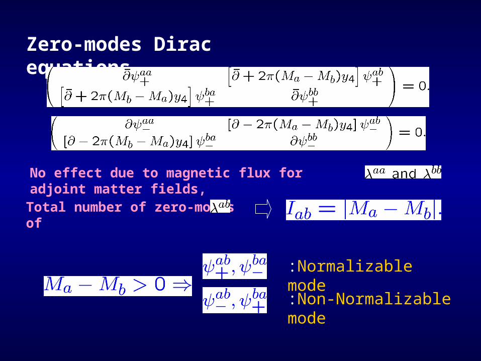
Zero-modes Dirac equations
Total number of zero-modes of
:Normalizable mode
:Non-Normalizable mode
No effect due to magnetic flux for adjoint matter fields,

4D chiral theory 4D chiral theory 10D spinor 10D spinor light-cone 8s light-cone 8s even number of minus signseven number of minus signs 11stst ⇒ ⇒ 4D, the other ⇒4D, the other ⇒ 6D space6D space If all of appear If all of appear in 4D theory, that is non-chiral theory.in 4D theory, that is non-chiral theory. If for all torus, If for all torus, only only
appear for 4D helicity fixed.appear for 4D helicity fixed. ⇒ ⇒ 4D chiral theory 4D chiral theory
),(
, , baab NN

U(8) SYM theory on T6U(8) SYM theory on T6
Pati-Salam group up to U(1) factorsPati-Salam group up to U(1) factors
Three families of matter fields Three families of matter fields
with many Higgs fieldswith many Higgs fields
2,1,41,2,4
3
2
1
3
2
1
0
0
2
N
N
N
zz
m
m
m
iF
2 ,2 ,4 321 NNNRL UUU )2()2()4(
other tori for the 1)()(
first for the 3)()(
1321
21321
mmmm
Tmmmm
)2,1,4()1,2,4(
)2,2,1(

2-2. Wilson lines 2-2. Wilson lines Cremades, Ibanez, Cremades, Ibanez,
Marchesano, Marchesano, ’’04, 04, Abe, Choi, T.K. Ohki, Abe, Choi, T.K. Ohki, ‘‘0909
torus without magnetic fluxtorus without magnetic flux constant Ai constant Ai mass shift mass shift every modes massiveevery modes massive magnetic fluxmagnetic flux
the number of zero-modes is the same.the number of zero-modes is the same. the profile: f(y) the profile: f(y) f(y +a/M) f(y +a/M) with proper b.c.with proper b.c.
0 )(2
0 )(2
aMy
aMy

U(1)a*U(1)b theory U(1)a*U(1)b theory magnetic flux, Fa=2πM, Fb=0magnetic flux, Fa=2πM, Fb=0
Wilson line, Aa=0, Ab=CWilson line, Aa=0, Ab=C
matter fermions with U(1) charges, matter fermions with U(1) charges, (Qa,Qb)(Qa,Qb)
chiral spectrum, chiral spectrum,
for Qa=0, massive due to nonvanishing for Qa=0, massive due to nonvanishing WLWL
when MQa >0, the number of zero-modeswhen MQa >0, the number of zero-modes
is MQa.is MQa.
zero-mode profile is shifted depending zero-mode profile is shifted depending
on Qb, on Qb,
))/(( )( ab MQCQzfzf

Pati-Salam modelPati-Salam model
Pati-Salam group Pati-Salam group
WLs along a U(1) in U(4) and a U(1) in U(2)R WLs along a U(1) in U(4) and a U(1) in U(2)R
=> Standard gauge group up to U(1) factors=> Standard gauge group up to U(1) factors
(the others are (the others are massive.)massive.)
U(1)Y is a linear combination.U(1)Y is a linear combination.
2,1,41,2,4
3
2
1
3
2
1
0
0
2
N
N
N
zz
m
m
m
iF 2 ,2 ,4 321 NNN
RL UUU )2()2()4(
other tori for the 1)()(
first for the 3)()(
1321
21321
mmmm
Tmmmm
3)1()2()3( UUU LC

PS => SMPS => SMZero modes corresponding to Zero modes corresponding to
three families of matter fields three families of matter fields
remain after introducing WLs, but their profiles splitremain after introducing WLs, but their profiles split
(4,2,1)(4,2,1)
Q LQ L
)2,1,4()1,2,4(
)1,1,1()1,1,1()1,1,3()1,1,3()2,1,4(
)1,2,1()1,2,3()1,2,4(

Other modelsOther modelsWe can start with 10D SYM, We can start with 10D SYM, 6D SYM (+ hyper multiplets),6D SYM (+ hyper multiplets), or non-SUSY models (+ matter fields )or non-SUSY models (+ matter fields ) with gauge groups, with gauge groups,
U(N), SO(N), E6, E7,E8,...U(N), SO(N), E6, E7,E8,...
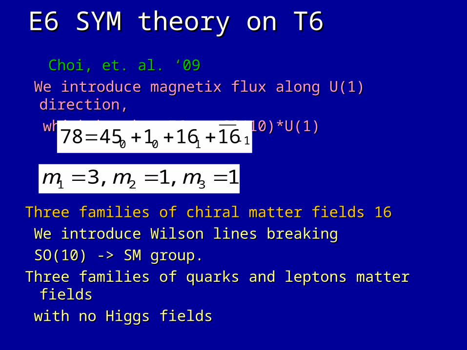
E6 SYM theory on T6E6 SYM theory on T6 Choi, et. al. Choi, et. al. ‘‘0909
We introduce magnetix flux along U(1) direction, We introduce magnetix flux along U(1) direction,
which breaks E6 -> SO(10)*U(1)which breaks E6 -> SO(10)*U(1)
Three families of chiral matter fields 16Three families of chiral matter fields 16
We introduce Wilson lines breaking We introduce Wilson lines breaking
SO(10) -> SM group.SO(10) -> SM group.
Three families of quarks and leptons matter fields Three families of quarks and leptons matter fields
with no Higgs fieldswith no Higgs fields
1100 161614578
1 ,1 ,3 321 mmm

Splitting zero-mode profilesSplitting zero-mode profilesWilson lines do not change the Wilson lines do not change the
(generation) number of zero-modes, (generation) number of zero-modes, but change localization point.but change localization point.
1616
QQ ………… LL
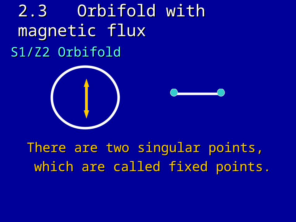
2.3 Orbifold with magnetic 2.3 Orbifold with magnetic fluxflux
S1/Z2 OrbifoldS1/Z2 Orbifold
There are two singular points, There are two singular points,
which are called fixed points.which are called fixed points.

OrbifoldsOrbifolds
T2/Z3 OrbifoldT2/Z3 Orbifold
There are three fixed points on Z3There are three fixed points on Z3 orbifoldorbifold
(0,0), (2/3,1/3), (1/3,2/3) su(3) root (0,0), (2/3,1/3), (1/3,2/3) su(3) root latticelattice
T2/Z4, T2/Z6T2/Z4, T2/Z6
Orbifold = D-dim. Torus /twistOrbifold = D-dim. Torus /twist
Torus = D-dim flat space/ lattice Torus = D-dim flat space/ lattice
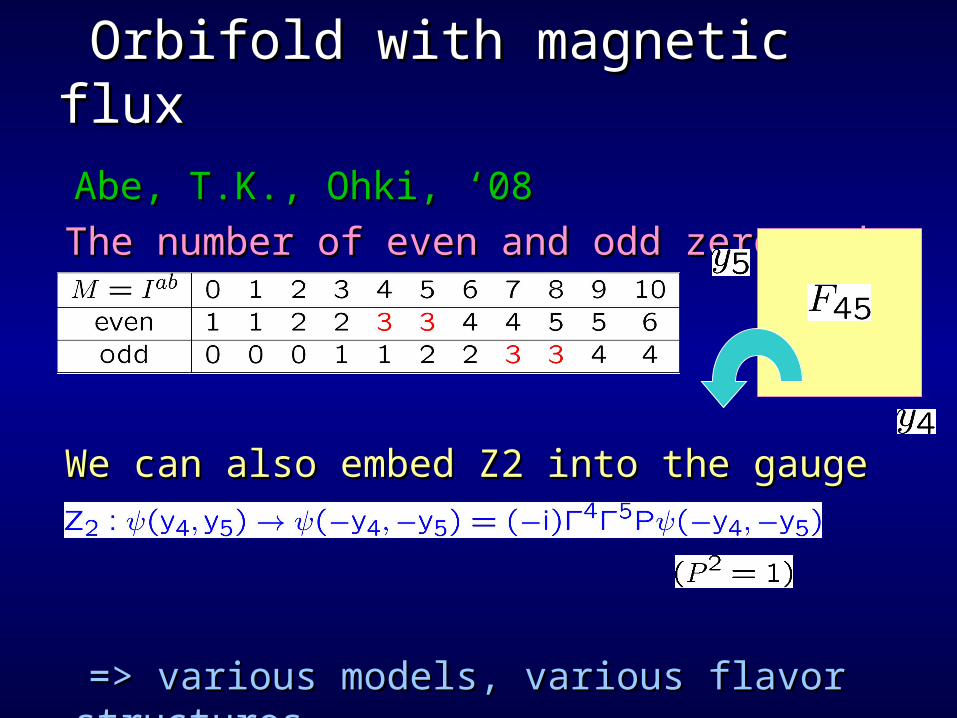
Orbifold with magnetic fluxOrbifold with magnetic flux Abe, T.K., Ohki, Abe, T.K., Ohki, ‘‘0808
The number of even and odd zero-modesThe number of even and odd zero-modes
We can also embed Z2 into the gauge We can also embed Z2 into the gauge space.space.
=> various models, various flavor => various models, various flavor structuresstructures

Wave functions
Wave function profile on toroidal background
For the case of M=3
Zero-modes wave functions are quasi-localized far away each other in extra dimensions. Therefore the hierarchirally small Yukawa couplings may be obtained.

Zero-modesZero-modes on orbifoldon orbifold
Adjoint matter fields are projected by Adjoint matter fields are projected by
orbifold projection.orbifold projection.
We have degree of freedom to We have degree of freedom to
introduce localized modes on fixed introduce localized modes on fixed points points
like quarks/leptons and higgs fields.like quarks/leptons and higgs fields.

Zero-modesZero-modes onon ZN orbifoldZN orbifold
Similarly we can discuss Similarly we can discuss
2D ZN orbifolds with magnetic fluxes 2D ZN orbifolds with magnetic fluxes
for N=2,3,4 and 6.for N=2,3,4 and 6.
Abe, Fujimoto, T.K., Miura, Nishiwaki, Abe, Fujimoto, T.K., Miura, Nishiwaki,
Sakamoto, Sakamoto, arXiv:1309.4925arXiv:1309.4925

3.3. N-point couplings N-point couplings and flavor symmetries and flavor symmetries
The N-point couplings are obtained by The N-point couplings are obtained by overlap integral of their zero-mode w.f.overlap integral of their zero-mode w.f.’’s.s.
)()()(2 zzzzdgY kP
jN
iM
54 iyyz

Moduli Moduli Torus metric Torus metric
AreaArea
We can repeat the previous analysis. We can repeat the previous analysis.
Scalar and vector fields have the same Scalar and vector fields have the same
wavefunctions.wavefunctions.
Wilson moduli Wilson moduli
shift of w.f.shift of w.f.
zdzdRds 22 )2(2
)( )(
zz
M
yxz
Im4 22RA

Zero-modes Zero-modes Cremades, Ibanez, Marchesano, Cremades, Ibanez, Marchesano, ‘‘0404
Zero-mode w.f. = gaussian x theta-Zero-mode w.f. = gaussian x theta-functionfunction
up to normalization factor up to normalization factor
),(0
/)]Im(exp[)( iMMz
MjzMziNz M
jM
,)()()(1
NM
m
MmjiNMijm
jN
iM zyzz
))(,0(0
))(/()(NMiMN
NMMNMNmMjNiyijm
MjNM ,,1 factor,ion normalizat:

Products of wave functions Products of wave functions
products of zero-modes = zero-modesproducts of zero-modes = zero-modes
NMNM
NM
N
M
yNM
Ny
My
)(
)( ,0 )(2
,0 2
,0 2

3-point couplings3-point couplings Cremades, Ibanez, Marchesano, Cremades, Ibanez, Marchesano, ‘‘0404
The 3-point couplings are obtained by The 3-point couplings are obtained by
overlap integral of three zero-mode w.f.overlap integral of three zero-mode w.f.’’s.s.
up to normalization factor up to normalization factor
ikkM
iM zzzd *2 )()(
*2 )()()( zzzzdY k
NMjN
iMijk
NM
mijmkmMjiijk yY
1,

Selection rule Selection rule
Each zero-mode has a Zg charge, Each zero-mode has a Zg charge,
which is conserved in 3-point couplings.which is conserved in 3-point couplings.
up to normalization factor up to normalization factor
)(, NMkmMjikmMji
))(,0(0
))(/()(NMiMN
NMMNMNmMjNiyijm
),gcd( when mod NMggkji

4-point couplings4-point couplings Abe, Choi, T.K., Ohki, Abe, Choi, T.K., Ohki, ‘‘0909 The 4-point couplings are obtained by The 4-point couplings are obtained by overlap integral of four zero-mode w.f.overlap integral of four zero-mode w.f.’’s.s. splitsplit
insert a complete setinsert a complete set
up to normalization factor up to normalization factor for K=M+Nfor K=M+N
*2 )()()()( zzzzzdY l
PNMkP
jN
iMijkl
modes all
*)'()()'( zzzz n
KnK
*22 )'()'()'()()(' zzzzzzzzdd l
PNMkP
jN
iM
lsksijs
lijk yyY

4-point couplings: another 4-point couplings: another splittingsplitting
i k i ki k i k
t t
j s l j lj s l j l
*22 )'()'()'()()(' zzzzzzzzdd l
PNMjN
kP
iM
ltjtikt
lijk yyY
ltjtikt
lijk yyY lsksij
slijk yyY
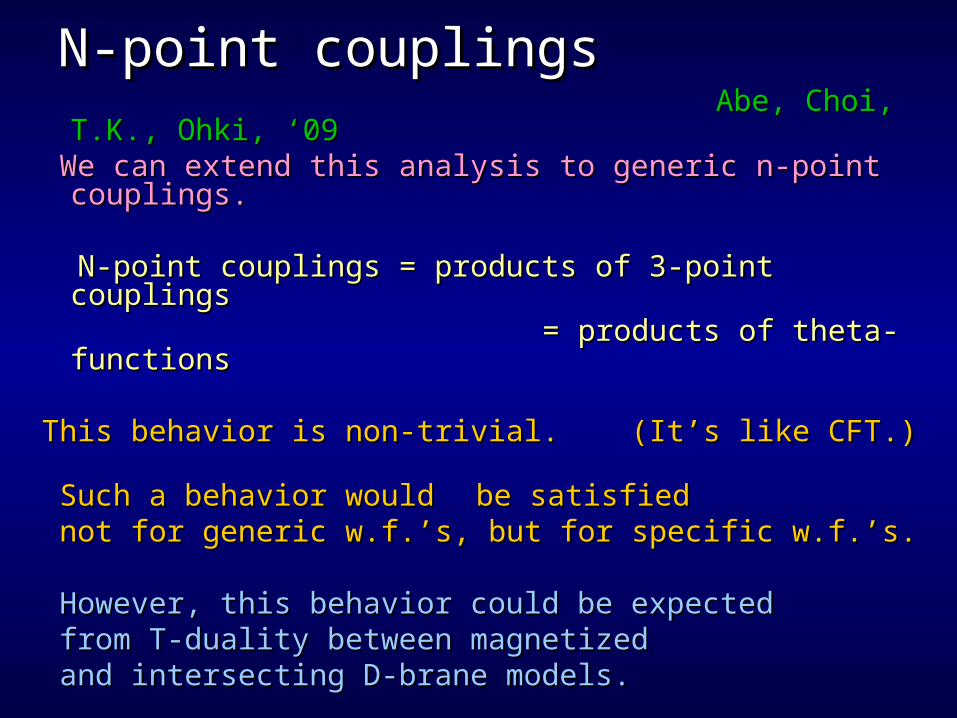
N-point couplingsN-point couplings Abe, Choi, T.K., Ohki, Abe, Choi, T.K., Ohki, ‘‘09 09
We can extend this analysis to generic n-point We can extend this analysis to generic n-point
couplings.couplings. N-point couplings = products of 3-point N-point couplings = products of 3-point
couplingscouplings = products of theta-functions= products of theta-functions
This behavior is non-trivial. (ItThis behavior is non-trivial. (It ’’s like CFT.) s like CFT.) Such a behavior wouldSuch a behavior would be satisfied be satisfied not for generic w.f.not for generic w.f.’’s, but for specific w.f.s, but for specific w.f.’’s.s. However, this behavior could be expected However, this behavior could be expected from T-duality between magnetized from T-duality between magnetized and intersecting D-brane models.and intersecting D-brane models.
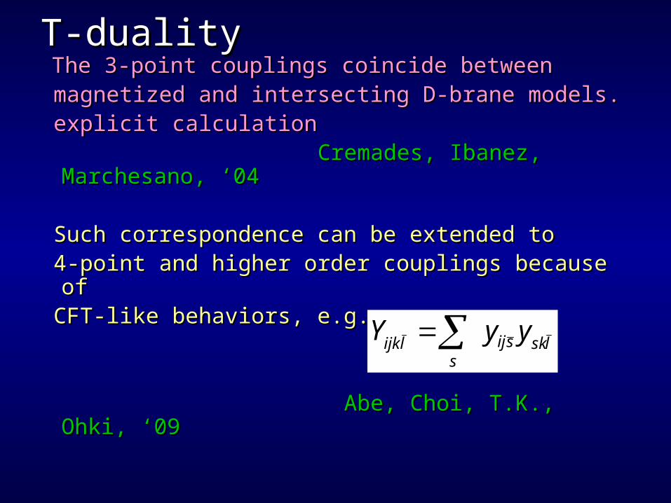
T-dualityT-duality The 3-point couplings coincide between The 3-point couplings coincide between magnetized and intersecting D-brane models. magnetized and intersecting D-brane models. explicit calculationexplicit calculation Cremades, Ibanez, Marchesano, Cremades, Ibanez, Marchesano, ‘‘0404
Such correspondence can be extended to Such correspondence can be extended to 4-point and higher order couplings because of 4-point and higher order couplings because of CFT-like behaviors, e.g., CFT-like behaviors, e.g.,
Abe, Choi, T.K., Ohki, Abe, Choi, T.K., Ohki, ‘‘09 09
lsksijs
lijk yyY

Non-Abelian discrete flavor Non-Abelian discrete flavor symmetrysymmetry
The coupling selection rule is controlled by The coupling selection rule is controlled by
Zg charges.Zg charges.
For M=g,For M=g, 1 2 1 2 g g
Effective field theory also has a cyclic permutation Effective field theory also has a cyclic permutation symmetry of g zero-modes. symmetry of g zero-modes.
These lead to non-Abelian flavor symmetires These lead to non-Abelian flavor symmetires
such as D4 and Δ(27)such as D4 and Δ(27) Abe, Choi, T.K, Ohki, ‘09Abe, Choi, T.K, Ohki, ‘09 Cf. heterotic orbifolds, Cf. heterotic orbifolds, T.K. Raby, Zhang, T.K. Raby, Zhang, ’’0404
T.K. Nilles, Ploger, Raby, Ratz, T.K. Nilles, Ploger, Raby, Ratz, ‘‘0606
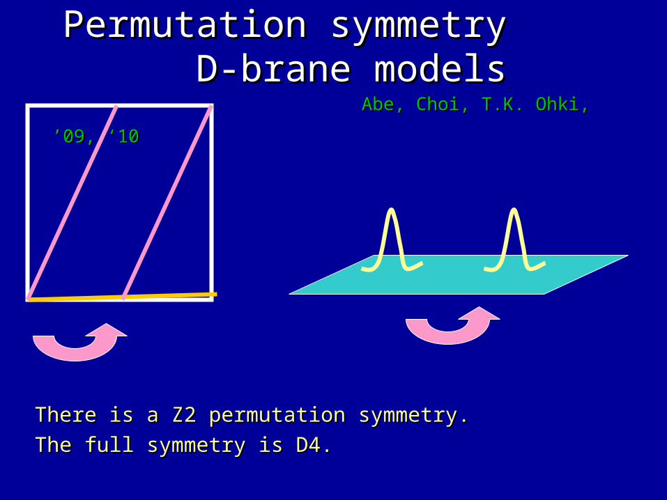
Permutation symmetryPermutation symmetry D-brane models D-brane models
Abe, Choi, T.K. Ohki, Abe, Choi, T.K. Ohki, ’’09, 09, ‘‘1010
There is a Z2 permutation symmetry.There is a Z2 permutation symmetry.
The full symmetry is D4.The full symmetry is D4.

Permutation symmetry Permutation symmetry D-brane models D-brane models Abe, Choi, T.K. Ohki, Abe, Choi, T.K. Ohki, ’’09, 09, ‘‘1010
geometrical symm. Full symm. geometrical symm. Full symm. Z3 Δ(27) Z3 Δ(27)
S3 Δ(54)S3 Δ(54)

intersecting/magnetized intersecting/magnetized D-brane models D-brane models Abe, Choi, T.K. Ohki, Abe, Choi, T.K. Ohki, ’’09, 09, ‘‘1010
generic intersecting number ggeneric intersecting number g
magnetic fluxmagnetic flux
flavor symmetry is a closed algebra of flavor symmetry is a closed algebra of
two Zgtwo Zg’’s.s.
and Zg permutationand Zg permutation
Certain case: Zg permutation larger symm. Certain case: Zg permutation larger symm.
Like Dg Like Dg
gi
g
e /2
1
, ,
1
0100
0010

Magnetized brane-modelsMagnetized brane-models
Magnetic flux M D4Magnetic flux M D4 2 22 2 4 14 1++++ + 1 + 1+- +- +1+1-+-+ + 1 + 1-- -- ・・・ ・・・
・・・・・・・・・ ・・・・・・・・・ Magnetic flux M Δ(27) (Δ(54))Magnetic flux M Δ(27) (Δ(54)) 3 33 311
6 2 x 36 2 x 31 1
9 ∑19 ∑1nn n=1, n=1,……,9 ,9 (1(111+∑2+∑2nn n=1, n=1,……,4),4) ・・・ ・・・
・・・・・・・・・ ・・・・・・・・・

Non-Abelian discrete flavor Non-Abelian discrete flavor symm.symm.
Recently, in field-theoretical model building, Recently, in field-theoretical model building,
several types of discrete flavor symmetries have several types of discrete flavor symmetries have
been proposed with showing interesting results, been proposed with showing interesting results,
e.g. S3, D4, A4, S4, Q6, Δ(27), ......e.g. S3, D4, A4, S4, Q6, Δ(27), ......
Review: e.g Review: e.g
Ishimori, T.K., Ohki, Okada, Shimizu, Tanimoto Ishimori, T.K., Ohki, Okada, Shimizu, Tanimoto ‘‘1010
⇒ ⇒ large mixing angles large mixing angles
one Ansatz: tri-bimaximalone Ansatz: tri-bimaximal
2/13/16/1
2/13/16/1
03/13/2

3.2 Applications of couplings3.2 Applications of couplings We can obtain quark/lepton masses and mixing angles. We can obtain quark/lepton masses and mixing angles.
Yukawa couplings depend on volume moduli, Yukawa couplings depend on volume moduli,
complex structure moduli and Wilson lines.complex structure moduli and Wilson lines.
By tuning those values, we can obtain semi-realistic results.By tuning those values, we can obtain semi-realistic results.
Ratios depend on complex structure moduli Ratios depend on complex structure moduli
and Wilson lines.and Wilson lines.
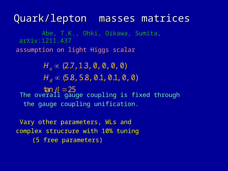
Quark/lepton masses matricesQuark/lepton masses matrices Abe, T.K., Ohki, Oikawa, Sumita, arXiv:1211.437Abe, T.K., Ohki, Oikawa, Sumita, arXiv:1211.437
assumption on light Higgs scalar assumption on light Higgs scalar
The overall gauge coupling is fixed through The overall gauge coupling is fixed through
the gauge coupling unification.the gauge coupling unification.
Vary other parameters, WLs and Vary other parameters, WLs and
complex strucrure with 10% tuningcomplex strucrure with 10% tuning
(5 free parameters)(5 free parameters)
25 tan
)0 ,0 ,1.0 ,1.0 ,8.5 ,8.5(
)0 ,0 ,0 ,0 ,3.1 ,7.2(
d
u
H
H

Quark/lepton masses and mixing Quark/lepton masses and mixing anglesangles Abe, T.K., Ohki, Oikawa, Sumita, arXiv:1211.437Abe, T.K., Ohki, Oikawa, Sumita, arXiv:1211.437
ExampleExample
Flavor is still a challenging issue.Flavor is still a challenging issue.,5.0
,60
,3
002.0,04.0,21.0
3,3
150,0.1
6,170
MeVM
MeVM
GeVM
VVV
MeVMMeVM
MeVMGeVM
GeVMGeVM
e
ubcbus
du
sc
bt
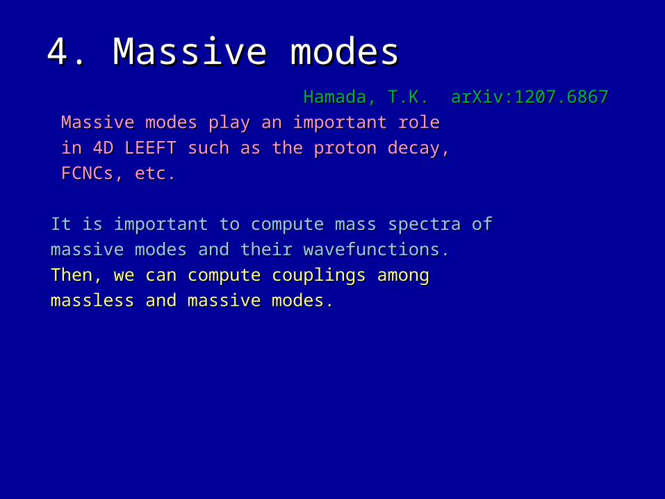
4. Massive modes4. Massive modes Hamada, T.K. arXiv:1207.6867Hamada, T.K. arXiv:1207.6867
Massive modes play an important role Massive modes play an important role
in 4D LEEFT such as the proton decay, in 4D LEEFT such as the proton decay,
FCNCs, etc.FCNCs, etc.
It is important to compute mass spectra of It is important to compute mass spectra of
massive modes and their wavefunctions.massive modes and their wavefunctions.
Then, we can compute couplings among Then, we can compute couplings among
massless and massive modes.massless and massive modes.

Fermion massive modes Fermion massive modes Two components are mixed.Two components are mixed. 2D Laplace op. 2D Laplace op.
algebraic relationsalgebraic relations
It looks like the quantum harmonic oscillator It looks like the quantum harmonic oscillator
n
nn
n
n mDD
DD
,
,2
,
,
0
0
AMDDADMD
AMDD
/4],[ ,/4],[
/4],[
2/},{ DD
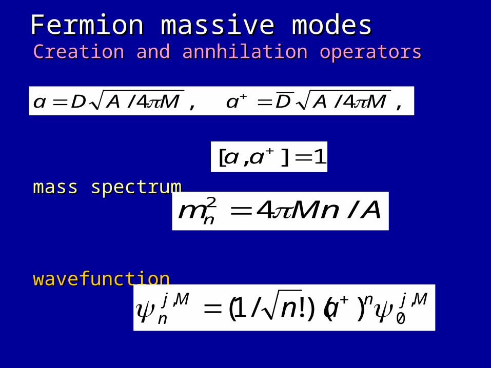
Fermion massive modes Fermion massive modes Creation and annhilation operatorsCreation and annhilation operators
mass spectrummass spectrum
wavefunction wavefunction
,4/ ,4/ MADaMADa
AMnmn /42
1],[ aa
MjnMjn an ,
0, ))(!/1(

Fermion massive modes Fermion massive modes explicit wavefunctionexplicit wavefunction
Hn: Hermite functionHn: Hermite function
Orthonormal condition: Orthonormal condition:
)/(Re)Im/Im/22(Re
)Im/Im/(Imexp[),( 2,
MjkMizMjkzMi
zMjkMzMjk
njkMkMj
nzd *,,2 )(
Im/)Im(/Im2
),()!2(
)Im2( ,2/1
4/1,
zMjkMH
zAn
M
n
k
Mjkn
Mjn

Scalar and vector modes Scalar and vector modes The wavefunctions of scalar and vector fields The wavefunctions of scalar and vector fields are the same as those of spinor fields.are the same as those of spinor fields. Mass spectrumMass spectrum scalar scalar vector vector Scalar modes are always massive on T2.Scalar modes are always massive on T2. The lightest vector mode along T2, The lightest vector mode along T2, i.e. the 4D scalar, is tachyonic on T2.i.e. the 4D scalar, is tachyonic on T2.
Such a vector mode can be massless on T4 or Such a vector mode can be massless on T4 or T6. T6.
AnMmn /)12(22 AnMmn /)12(22
)///(2 3322112 AMAMAMm
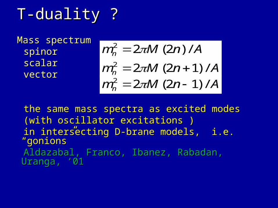
T-duality ? T-duality ? Mass spectrumMass spectrum spinor spinor scalar scalar vector vector
the same mass spectra as excited modes the same mass spectra as excited modes (with oscillator excitations ) (with oscillator excitations ) in intersecting D-brane models, i.e. “gonions” in intersecting D-brane models, i.e. “gonions” Aldazabal, Franco, Ibanez, Rabadan, Uranga, ‘01 Aldazabal, Franco, Ibanez, Rabadan, Uranga, ‘01
AnMm
AnMm
n
n
/)12(2
/)2(22
2
AnMmn /)12(22

Products of wavefunctions Products of wavefunctions explicit wavefunctionexplicit wavefunction
See also See also Berasatuce-Gonzalez, Camara, Marchesano, Berasatuce-Gonzalez, Camara, Marchesano,
Regalado, Uranga, ‘12 Regalado, Uranga, ‘12
Derivation: Derivation: products of zero-mode wavefunctionsproducts of zero-mode wavefunctionsWe operate creation operators on both LHS We operate creation operators on both LHS and RHS. and RHS.
),0(
)!!/()!()!(
)()1(
)( ,
2121
2/)1(2/)(2/)(
21
21122
21
MNNMNMmNjMisnn
nnsnsnsnsnn
ijms
nnsnns
MNMNCCy
,)()()(1
,
0 0
,,1 2
21
NM
m
MNMmjis
ijms
n n
s
Njn
Min zyzz
,)()()(1
,,,
NM
m
NMMmjiijm
NjMi zyzz

3-point couplings including 3-point couplings including higher modes higher modes
The 3-point couplings are obtained by The 3-point couplings are obtained by
overlap integral of three wavefunctions.overlap integral of three wavefunctions.
(flavor) selection rule (flavor) selection rule
is the same as one for the massless is the same as one for the massless modes.modes.
(mode number) selection rule (mode number) selection rule
sikMj
sMi zzzd
*,,2 )()(
*,,,2 )()()(
321321zzzzdY NMk
nMj
nNi
nkij
nnn
NM
m
ijmsnskmMji
n n
s
kijnnn yY
1,,
0 03
1 2
321
Mkji mod
213 nnn

3-point couplings:3-point couplings:2 zero-modes and one higher 2 zero-modes and one higher mode mode
3-point coupling3-point coupling
031 nn 213 nnn
),0()( )( ,)(2/)1(2/
2
22 MNNMjNMMkn
nn MNNY

Higher order couplings including Higher order couplings including higher modes higher modes
Similarly, we can compute higher order couplings Similarly, we can compute higher order couplings
including zero-modes and higher modes. including zero-modes and higher modes.
They can be written by the sum over They can be written by the sum over
products of 3-point couplings.products of 3-point couplings.
*,,,2 )()()(
21zzzzdY Pk
nMj
nNi
n m
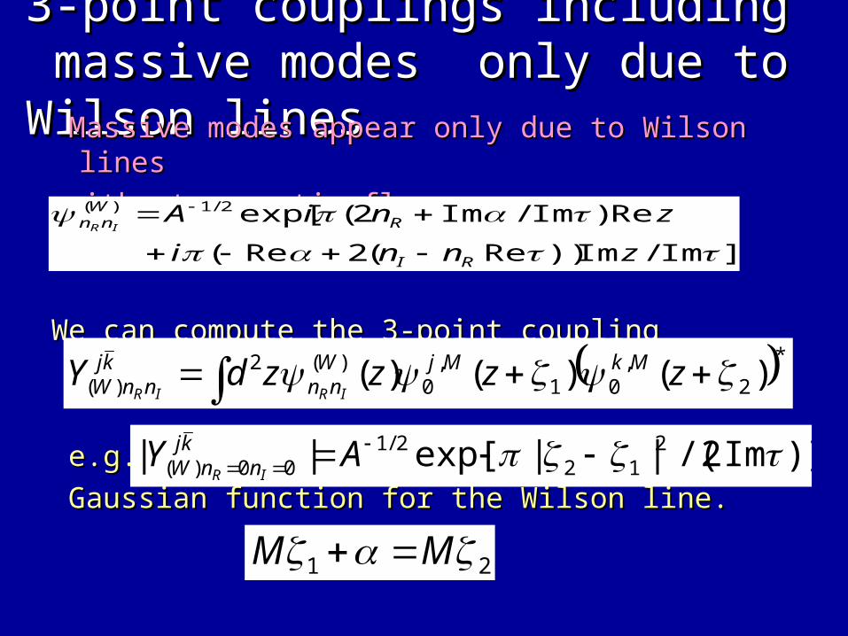
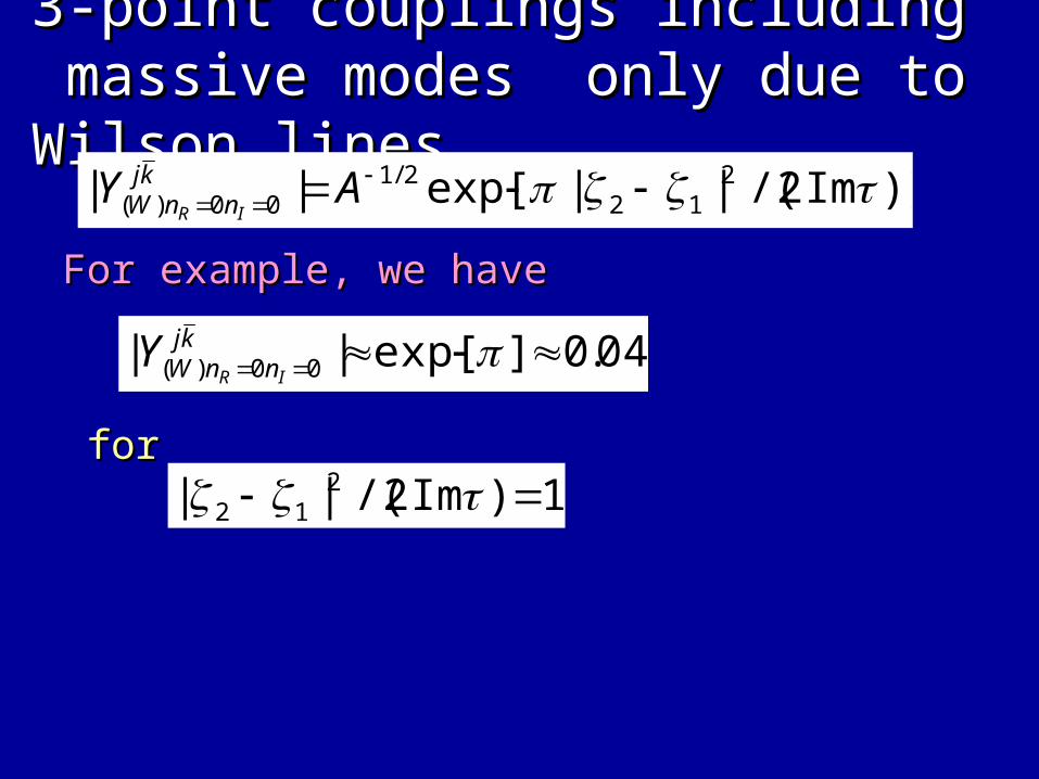
3-point couplings including 3-point couplings including massive modes only due to massive modes only due to Wilson linesWilson lines Massive modes appear only due to Wilson lines Massive modes appear only due to Wilson lines
without magnetic fluxwithout magnetic flux
We can compute the 3-point couplingWe can compute the 3-point coupling
e.g. e.g.
Gaussian function for the Wilson line. Gaussian function for the Wilson line.
21 MM
)]Im2/(||exp[|| 212
2/100)( AY kj
nnW IR
]Im/Im))Re(2Re(
Re)Im/Im2(exp[2/1)(
znni
zniA
RI
RW
nn IR
*
2,
01,
0)(2
)( )()()( zzzzdY MkMjWnn
kjnnW IRIR
3-point couplings including 3-point couplings including massive modes only due to massive modes only due to Wilson linesWilson lines
For example, we have For example, we have
for for
)]Im2/(||exp[|| 212
2/100)( AY kj
nnW IR
1)Im2/(|| 212
04.0]exp[|| 00)( kjnnW IR
Y

Several couplingsSeveral couplings Similarly, we can compute the 3-point Similarly, we can compute the 3-point
couplings couplings
including higher modes including higher modes
Furthermore, we can compute higher order Furthermore, we can compute higher order
couplings including several modes, similarly.couplings including several modes, similarly.
*,,)(2
)( )()()(2121
zzzzdY Mkn
Mj
n
Wnn
kjnnWnn IRIR
*,,)(2 )()()(
21zzzzdY Mk
nMj
n
Wnn IR

4.2 Phenomenological 4.2 Phenomenological applicationsapplicationsIn 4D SU(5) GUT, In 4D SU(5) GUT,
The heavy X boson couples with quarks and leptons The heavy X boson couples with quarks and leptons
by the gauge coupling. by the gauge coupling.
Their couplings do not change even after GUT Their couplings do not change even after GUT breaking breaking
and it is the gauge coupling.and it is the gauge coupling.
However, that changes in our models.However, that changes in our models.

Phenomenological applicationsPhenomenological applicationsFor example, For example,
we consider the SU(5)xU(1) GUT model we consider the SU(5)xU(1) GUT model
and we put magnetic flux along extra U(1).and we put magnetic flux along extra U(1).
The 5 matter field has the U(1) charge q, The 5 matter field has the U(1) charge q,
and the quark and lepton in 5 are quasi-localized and the quark and lepton in 5 are quasi-localized
at the same place.at the same place.
Their coupling with the X boson is given by Their coupling with the X boson is given by
the gauge coupling before the GUT breaking.the gauge coupling before the GUT breaking.

SU(5) => SMSU(5) => SMWe break SU(5) by the WL along the U(1)Y direction.We break SU(5) by the WL along the U(1)Y direction.
The X boson becomes massive. The X boson becomes massive.
The quark and lepton in 5 remain massless, but their The quark and lepton in 5 remain massless, but their
profiles split each other. profiles split each other.
Their coupling with X is not equal to the gauge Their coupling with X is not equal to the gauge coupling, coupling,
but includes the suppression factor but includes the suppression factor
55
Q LQ L
04.0]exp[|| 00)( kjnnW IR
Y

Proton decay Proton decay Similarly, the couplings of the X boson with quarks and Similarly, the couplings of the X boson with quarks and
leptons in the 10 matter fields can be suppressed. leptons in the 10 matter fields can be suppressed.
That is important to avoid the fast proton decay. That is important to avoid the fast proton decay.
The proton life time would drastically The proton life time would drastically
change by the factor, change by the factor,
)1010( 54 O
04.0]exp[|| 00)( kjnnW IR
Y
Other aspects Other aspects Other couplings including massless and massive modes Other couplings including massless and massive modes
can be suppressed and those would be important , can be suppressed and those would be important ,
such as right-handed neutrino masses and such as right-handed neutrino masses and
off-diagonal terms of Kahler metric, etc.off-diagonal terms of Kahler metric, etc.
Threshold corrections on the gauge couplings, Threshold corrections on the gauge couplings,
Kahler potential after integrating out massive modesKahler potential after integrating out massive modes

5. Flavor and Higgs sector5. Flavor and Higgs sector
factorizable magnetic fluxes, factorizable magnetic fluxes,
non-vanishing F45, F67, F89 non-vanishing F45, F67, F89
Three generations of both left-handed and Three generations of both left-handed and
right-handed quarks originate only from right-handed quarks originate only from
the same 2D torus.the same 2D torus.
-> the number of higgs = 6.-> the number of higgs = 6.
Δ(27) flavor symmetriesΔ(27) flavor symmetries
three families = triplet three families = triplet
higgs fields = 2x (triplet)higgs fields = 2x (triplet)

Flavor and Higgs sectorFlavor and Higgs sector
Abe, T.K. , Ohki, Sumita, Tatsuta ’ 1307.1831 Abe, T.K. , Ohki, Sumita, Tatsuta ’ 1307.1831
non-factorizable magnetic fluxes, non-factorizable magnetic fluxes,
non-vanishing F45, F67, F89 and F46, ………..non-vanishing F45, F67, F89 and F46, ………..
Three generations of both left-handed and Three generations of both left-handed and
right-handed quarks originate from 4D torusright-handed quarks originate from 4D torus
-> several patterns of higgs sectors, -> several patterns of higgs sectors,
one pair, two , …….one pair, two , …….
Δ(27) flavor symmetries are vilolated.Δ(27) flavor symmetries are vilolated.

Flavor and Higgs sectorFlavor and Higgs sector
In most of cases, In most of cases,
there are multi higgs fields.there are multi higgs fields.
in a certain case, Δ(27) flavor symmetryin a certain case, Δ(27) flavor symmetry
What is phenomenological aspects What is phenomenological aspects
of multi higgs fields, e.g. in LHC ? of multi higgs fields, e.g. in LHC ?

SummarySummaryWe have studiedWe have studied phenomenological aspects phenomenological aspects of magnetized brane models.of magnetized brane models.
Model building from U(N), E6, E7, E8Model building from U(N), E6, E7, E8
N-point couplings are comupted.N-point couplings are comupted. 4D effective field theory has non-Abelian 4D effective field theory has non-Abelian
flavor flavor symmetries, e.g. D4, Δ(27).symmetries, e.g. D4, Δ(27). Orbifold background with magnetic flux is Orbifold background with magnetic flux is also important.also important.

Further studiesFurther studiesDerivation of realistic values of quark/lepton Derivation of realistic values of quark/lepton masses and mixing angles.masses and mixing angles. Applications of flavor symmetries Applications of flavor symmetries and studies on their anomaliesand studies on their anomalies
Phenomenological aspects of massive modesPhenomenological aspects of massive modes


