
STYRELSEN FÖR
VINTERSJÖFARTSFORSKNING
WINTER NAVIGATION RESEARCH BOARD
Research Report No 70 Juhani Hämäläinen
PLASTIC DEFORMATION SIMULATIONS OF PROPELLER BLADES Finnish Transport Safety Agency Swedish Maritime Administration Finnish Transport Agency Swedish Transport Agency Finland Sweden

Talvimerenkulun tutkimusraportit – Winter Navigation Research Reports ISSN 2342-4303 ISBN 978-952-311-019-9
FOREWORD In its report no 70, the Winter Navigation Research Board presents the outcome of the project on plastic deformation simulations of propeller blades. According to the Finnish-Swedish Ice Class Rules, 2008, a propeller blade of a ship operating in ice must fail at a load given in the ice class regulations. This force is placed on the propeller blade at distance of 0.8R from the blade root with 2/3 spindle arm from the leading/trailing edge of the propeller blade. In this study two typical propeller blades were modelled using finite element method (FEM) and the ultimate failure load was calculated at 0.8R with spindle arms of 1/3 and 2/3. These results were compared to analytically calculated ones. The Winter Navigation Research Board warmly thanks Mr. Juhani Hämäläinen for this report. Helsinki and Norrköping June 2014 Jorma Kämäräinen Peter Fyrby Finnish Transport Safety Agency Swedish Maritime Administration Tiina Tuurnala Stefan Eriksson Finnish Transport Agency Swedish Transport Agency


RESEARCH REPORT VTTR0762310
Plastic deformation simulations of propeller blades
Authors: Juhani Hämäläinen
Confidentiality: Public
RESEARCH REPORT VTTR07623101 (46)
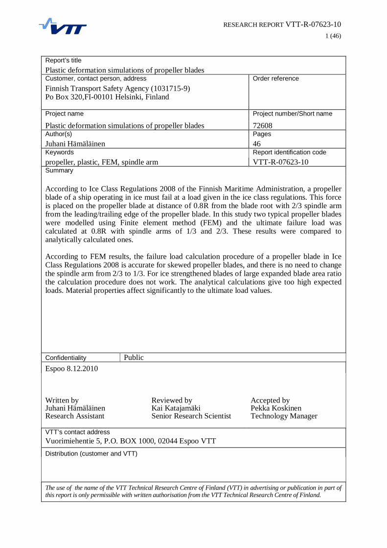
Report’s titlePlastic deformation simulations of propeller bladesCustomer, contact person, address Order referenceFinnish Transport Safety Agency (10317159)Po Box 320,FI00101 Helsinki, Finland
Project name Project number/Short name
Plastic deformation simulations of propeller blades 72608Author(s) PagesJuhani Hämäläinen 46Keywords Report identification codepropeller, plastic, FEM, spindle arm VTTR0762310Summary
According to Ice Class Regulations 2008 of the Finnish Maritime Administration, a propellerblade of a ship operating in ice must fail at a load given in the ice class regulations. This forceis placed on the propeller blade at distance of 0.8R from the blade root with 2/3 spindle armfrom the leading/trailing edge of the propeller blade. In this study two typical propeller bladeswere modelled using Finite element method (FEM) and the ultimate failure load wascalculated at 0.8R with spindle arms of 1/3 and 2/3. These results were compared toanalytically calculated ones.
According to FEM results, the failure load calculation procedure of a propeller blade in IceClass Regulations 2008 is accurate for skewed propeller blades, and there is no need to changethe spindle arm from 2/3 to 1/3. For ice strengthened blades of large expanded blade area ratiothe calculation procedure does not work. The analytical calculations give too high expectedloads. Material properties affect significantly to the ultimate load values.
Confidentiality PublicEspoo 8.12.2010
Written byJuhani HämäläinenResearch Assistant
Reviewed byKai KatajamäkiSenior Research Scientist
Accepted byPekka KoskinenTechnology Manager
VTT’s contact addressVuorimiehentie 5, P.O. BOX 1000, 02044 Espoo VTTDistribution (customer and VTT)
The use of the name of the VTT Technical Research Centre of Finland (VTT) in advertising or publication in part ofthis report is only permissible with written authorisation from the VTT Technical Research Centre of Finland.

RESEARCH REPORT VTTR07623102 (46)
Contents
1. Introduction.............................................................................................................3
2. Description..............................................................................................................42.1. Analytical calculations – Ice class regulations propeller blade failure load......5
2.1.1. Loading ................................................................................................52.1.2. Load cases...........................................................................................62.1.3. Analytical failure loads and torques .....................................................7
3. Limitations ..............................................................................................................8
4. Finite element analysis ...........................................................................................94.1. Meshing and mesh quality ..............................................................................9
4.1.1. Loading and boundary conditions ......................................................104.2. Studied cases ...............................................................................................10
5. Results .................................................................................................................115.1. Ship 1............................................................................................................11
5.1.1. Load case 1 .......................................................................................115.1.2. Load case 2 .......................................................................................125.1.3. Ship 1 Plots........................................................................................14
5.2. Ship 2............................................................................................................165.2.1. Load case 1, leading edge.................................................................165.2.2. Load case 2, leading edge.................................................................165.2.3. Ship 2 Plots........................................................................................195.2.4. Load at trailing edge ..........................................................................215.2.5. Trailing edge, plots.............................................................................225.2.6. Load case 3 .......................................................................................235.2.7. Load case 3, plots..............................................................................25
5.3. Material property validation...........................................................................265.3.1. Ship 1.................................................................................................275.3.2. Ship 1, plots .......................................................................................315.3.3. Ship 2.................................................................................................335.3.4. Ship 2, plots .......................................................................................35
6. Conclusions..........................................................................................................41
7. Appendix...............................................................................................................427.1. A: Calculation model validation.....................................................................42
1.1.2 Meshing, loading and boundary conditions........................................431.1.3 Results...............................................................................................441.1.4 Conclusions .......................................................................................48

RESEARCH REPORT VTTR07623103 (46)
1. Introduction
The Finnish Maritime Administration issued 12/2008 Ice Class Regulations forShips operating in the Baltic Sea. The ultimate load resulting from propeller bladefailure is specified in these regulations, [1], p. 38 formula 6.25 This study focuseson the behaviour of the propeller blade in failure and verifies the formula 6.25using FEM1. The relevance of the load of the formula 6.25 is compared with theresults obtained by commercial software Abaqus FEA version 6.9EF1. Especiallythe spindle arm for calculations of the extreme blade spindle torque arm isexamined. According to [1] the spindle arm is taken as 2/3 of the distancebetween the axis of blade rotation and the leading/trailing edge at the 0.8R radius.Loaded areas are shown in Picture 1. The objective of this study was to findanswers to following questions:
• Does the formula 6.25 lead to over dimensioning of the propeller bladeand shaft line components?
• Can the spindle torque arm be reduced to 1/3?
Picture 1, Loaded areas of the blade
1 Finite Element Method (FEM) is a numerical technique for solving structural analysis problems.
RESEARCH REPORT VTTR07623104 (46)
2. Description
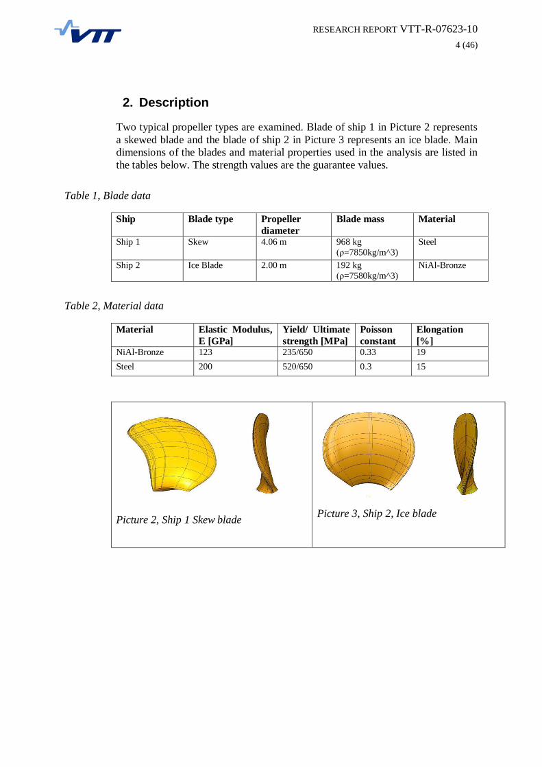
Two typical propeller types are examined. Blade of ship 1 in Picture 2 representsa skewed blade and the blade of ship 2 in Picture 3 represents an ice blade. Maindimensions of the blades and material properties used in the analysis are listed inthe tables below. The strength values are the guarantee values.
Table 1, Blade data
Ship Blade type Propellerdiameter
Blade mass Material
Ship 1 Skew 4.06 m 968 kg=7850kg/m^3)
Steel
Ship 2 Ice Blade 2.00 m 192 kg=7580kg/m^3)
NiAlBronze
Table 2, Material data
Material Elastic Modulus,E [GPa]
Yield/ Ultimatestrength [MPa]
Poissonconstant
Elongation[%]
NiAlBronze 123 235/650 0.33 19Steel 200 520/650 0.3 15
Picture 2, Ship 1 Skew blade Picture 3, Ship 2, Ice blade
RESEARCH REPORT VTTR07623105 (46)
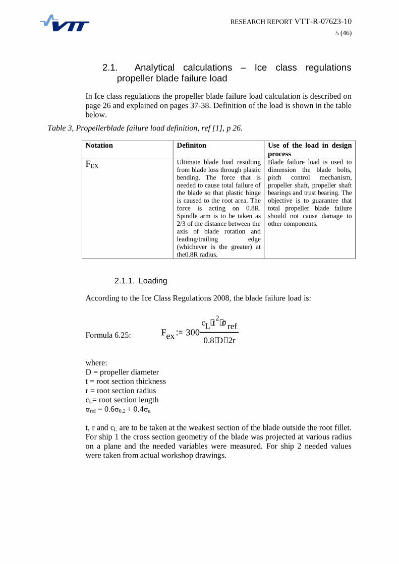
2.1. Analytical calculations – Ice class regulationspropeller blade failure load
In Ice class regulations the propeller blade failure load calculation is described onpage 26 and explained on pages 3738. Definition of the load is shown in the tablebelow.
Table 3, Propellerblade failure load definition, ref [1], p 26.
Notation Definiton Use of the load in designprocess
FEX Ultimate blade load resultingfrom blade loss through plasticbending. The force that isneeded to cause total failure ofthe blade so that plastic hingeis caused to the root area. Theforce is acting on 0.8R.Spindle arm is to be taken as2/3 of the distance between theaxis of blade rotation andleading/trailing edge(whichever is the greater) atthe0.8R radius.
Blade failure load is used todimension the blade bolts,pitch control mechanism,propeller shaft, propeller shaftbearings and trust bearing. Theobjective is to guarantee thattotal propeller blade failureshould not cause damage toother components.
2.1.1. Loading
According to the Ice Class Regulations 2008, the blade failure load is:
Formula 6.25:
where:D = propeller diametert = root section thicknessr = root section radiuscL= root section length
ref = 0.6 0.2 + 0.4 u
t, r and cL are to be taken at the weakest section of the blade outside the root fillet.For ship 1 the cross section geometry of the blade was projected at various radiuson a plane and the needed variables were measured. For ship 2 needed valueswere taken from actual workshop drawings.
Fex 300cL t2⋅ σref⋅
0.8 D⋅ 2r−:=

RESEARCH REPORT VTTR07623106 (46)
2.1.2. Load cases
The propeller blades are studied using three different load cases. Load case 1 is conducted byice class regulations 2008. Load case 2 is a proposal for alternative calculation of blade failureload. Load case 3 is considered in detail in results section. In general this load case was madeto make the ice blade deform plastically at the root section.
Table 4, Load cases
Load case applied area description1 2/3 of the distance
between the axis of bladerotation and theleading/trailing edge atthe 0.8R radius
Ice Class RegulationsBlade failure load 6.25
2 1/3 of the distancebetween the axis of bladerotation and theleading/trailing edge atthe 0.8R radius
Proposal for new loadingarea
3 A pressure on a surfacefrom 0.7R to 0.9R
For ship 2 ice blade; tofind the ultimate shaftpropeller bendingmoment.
Picture 4, Loaded areas

RESEARCH REPORT VTTR07623107 (46)
2.1.3. Analytical failure loads and torques
According to Ice class regulations 2008 formula 6.25 the failure forces werecalculated as described in section 2.1.1. By iteration the lowest failure load wasfound at 0.5R on both blades. Below mentioned quantities were used to calculatethe failure load for each blade.
Analytical moments MY and MZ were calculated to show the effect of the failureload at the propeller shaft and hub. The ice class regulations 2008 give nospecification for calculation of these moments and they are made only forillustrative purposes for this study. MY moment arms a and b and MZ momentarms 1/3B and 2/3B in Picture 4 are held constant. The analytically calculatedfailure loads and moments for specified load case are shown in Table 5.
Quantities for calculation Skewed blade
Propeller diameter D = 4.058 mR0.5 root section thickness t = 0.113 mR0.5 root section radius r = 1.014 mR0.5 root section length cL =1.165 m
Quantities for calculation Ice blade
Propeller diameter D = 1.99 mR0.5 root section thickness t = 0.082 mR0.5 root section radius r = 0.497 mR0.5 root section length cL = 0.786 m
Table 5, Reference loads and moments, A
Blade, Load Case ForceFex [MN]
BendingMY[MNm]
SpindleMZ[MNm]
Skew, Load case 1 2.10 3.18 1.23Skew, Load case 2 2.10 3.35 0.61Ice, Load case 1 1.04 0.77 0.31Ice, Load case 2 1.04 0.82 0.16Ice, Load case 3 1.04 0.83 0
Where:Fex= blade failure load by [1], p.38 fomula 6.25MY= analytical propeller shaft bending moment with constant moment arm a andb, see Picture 4MZ= analytical spindle moment with constant moment arm 1/3B or 2/3B specifiedby the load case, see Picture 4

RESEARCH REPORT VTTR07623108 (46)
3. Limitations
For ship 1 the measures used to calculate the ultimate blade failure load are takenfrom CAD models of the propeller blades, not from the actual workshop drawing.Thus minor error is evident, due to projection of the propeller crosssection etc.This has no effect on the magnitude of the strength of the blade.
The Abaqus material model is a bilinear stress strain curve with isotropichardening effect. This is a simplification from the actual elasticplastic model ofmetal materials. The elastic modulus of both materials is estimated to matchtypical values of the specific material. Other material data originates from actualworkshop data of the blades.
RESEARCH REPORT VTTR07623109 (46)
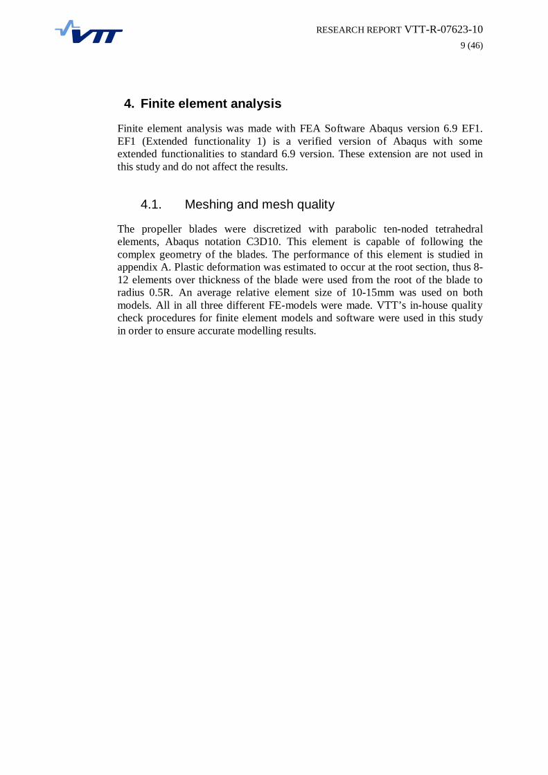
4. Finite element analysis
Finite element analysis was made with FEA Software Abaqus version 6.9 EF1.EF1 (Extended functionality 1) is a verified version of Abaqus with someextended functionalities to standard 6.9 version. These extension are not used inthis study and do not affect the results.
4.1. Meshing and mesh quality
The propeller blades were discretized with parabolic tennoded tetrahedralelements, Abaqus notation C3D10. This element is capable of following thecomplex geometry of the blades. The performance of this element is studied inappendix A. Plastic deformation was estimated to occur at the root section, thus 812 elements over thickness of the blade were used from the root of the blade toradius 0.5R. An average relative element size of 1015mm was used on bothmodels. All in all three different FEmodels were made. VTT’s inhouse qualitycheck procedures for finite element models and software were used in this studyin order to ensure accurate modelling results.

RESEARCH REPORT VTTR076231010 (46)
4.1.1. Loading and boundary conditions
In the FEmodels the loading is applied as a pressure on an area specified by theload case. In load cases 1 and 2 the loaded are is a circular area diameter of witchis 10% of the blade radius. In the load case 3 loaded area is bound between 0.7Rto 0.9R. Loaded areas are shown in Picture 1 and Picture 4. The pressure acts inthe direction of the blade surface normal and so it follows the deformation of theblade, this is regarded in the results. Calculation is force driven, and the pressureis gained until blade failure and beyond to see post failure behaviour of the blade.
In CAD environment the origin of the global coordinate system was placed at thepropeller shaft centre of rotation (COR). Coordinate system orientation is shownin Picture 5. The global xaxis is parallel and coincident with the propeller shaftaxis. The global zaxis is parallel and coincident with the blade turning axis. Allcoordinate directions in this report refer to global coordinate axes.
Propeller shaft was modelled with rigid element. The roots of the blades wererigidly bound to the global origin at the shaft COR. Boundary conditions areillustrated in Picture 6. Reaction forces and moments were printed at the COR.
4.2. Studied cases
Four different cases are discussed in this study. These are:1. Skewed blade failure load analysis2. Ice Blade failure load analysis3. Material property validation4. Element type validation, see Appendix A
Picture 5, Coordinate system Picture 6, Boundary conditions

RESEARCH REPORT VTTR076231011 (46)
5. Results
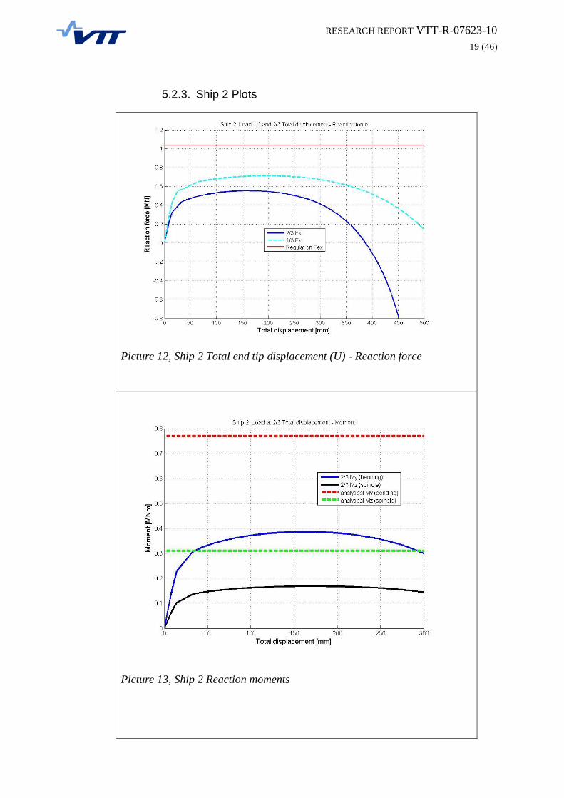
The propeller blades were calculated with their original materials in all load cases.In section 5.3 the materials were changed and the blades were calculated again.According to section 4.1.1 the orientation of the applied pressure changes as theblade deforms. Thus only FX reaction force components are shown in thedisplacement – reaction force plots. A resultant reaction force would give too highfailure load values. Other force components are regarded as secondary for thestrength of the blade. Displacement of the blade is given the as resultant of thedisplacement components at the most deflected area of the blade.
For example graphs in Picture 8 and Picture 12 illustrate the total displacement ofthe propeller blade end tip versus reaction force at the shaft spinning axis COR.The red line shows the failure load given by formula 6.25 in [1]. Totaldisplacement versus moment plots are made to illustrate loadings on the propellershaft and components related to the propeller hub. In moment plots Picture 9 andPicture 13 for example horizontal lines show the maximum bending momentscalculated analytically from failure load. MY is the bending around the global yaxis. This quantity represents propeller shaft bending. MZ is bending momentaround the global zaxis, this quantity represent spindle moment.
5.1. Ship 1
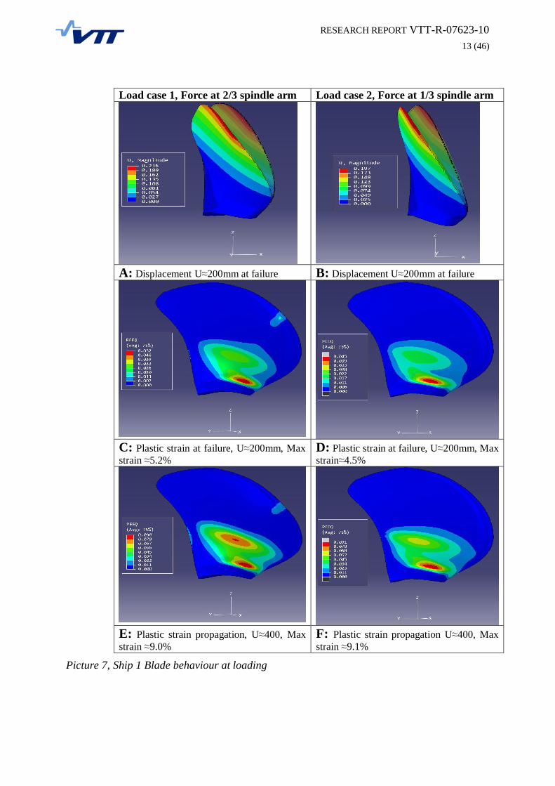
The deformation and the plastic behaviour of ship 1 is briefly shown in Picture 7.Load case 1 behaviour is seen in the left hand column, for load cases see Table 4.Right hand side column illustrates load case 2 behaviour respectively. Plastic areasize at failure was observed by relation of elements with plastic strain to totalamount of elements in the model.
5.1.1. Load case 1
Pictures 7A and 7B show the total deformation of the blade at failure load.Dashed geometry represent the initial shape of the propeller. Pictures 7C and 7 Dillustrate the area of plastic deformation at failure load. Solid blue line in Picture 8represents the result of load case 1. Reaction moments MY and MZ are presentedin Picture 9. Some values at failure are gathered in Table 6.
At failure two areas of plastic deformation can bee seen, picture 7C. These resultfrom simultaneous bending in YZplane and twisting around Zaxis. In general theplastic area occurs in the root section of the blade, below 0.5R. Once maximumfailure load is achieved, the plastic deformation propagates in the upper plasticarea, pictures 7E and 7F. Reaction force at failure achieves maximum value about16% below the analytical blade failure load. The reaction force reduces graduallyafter the maximum value. The maximum propeller shaft bending moment MY isabout 10% lower than could be expected by analytical calculations, see Table 5.The maximum propeller blade spindle moment MZ is about 3% higher thanexpected by analytical calculations. In load case 1 the analytical calculations givegood approximations for the propeller blade failure loads.

RESEARCH REPORT VTTR076231012 (46)
5.1.2. Load case 2
Load response of the blade is shown in Picture 8 by a dashed blue line and Picture10 illustrates reaction moments.
In load case 2, the propeller blade behaviour is very similar to load case 1, seeright hand column in Picture 7. The plastic area appears more horizontal than inload case 1 and its size is 5 percentage units smaller, see Table 6. The ultimatefailure load is about 3% lower than analytically calculated. The maximumpropeller shaft bending moment MY is about 4% lower than expected byanalytical calculations. The maximum propeller blade spindle moment MZ is 24 %higher than expected. Analytical calculations under estimate the actual spindlemoment but are able to estimate propeller shaft bending.
Table 6, Ship 1 plastic area size at failure
where:Plastic elem. = Number of plastic elements at failure load, plasticity limits [0.5%6%]Total elem. = Number of total elements in the FEmodelRFmax = Maximum reaction force in Picture 8RM = Maximum reaction moments in Picture 9 and Picture 10MY = analytical moment, Table 5MZ = analytical moment, Table 5Fex = Blade failure load, Table 5
Blade,Load case
Plasticelem./totalelem.
Plasticelements [%]
ForceRFmax /Fex
Force[%]
BendingRMY/ MY
Bending[%]
SpindleRMz/ Mz
Spindle[%]
Skew,Load case 1
88499/254300 34.0 % 1.975/2.10 94.2% 2.87/3.18 90.2% 1.29/1.23 102%
Skew,Load case 2
73789/254300 29.0% 2.034/ 2.10 96.9% 3.22/3.35 96.2% 0.76/0.61 124%
RESEARCH REPORT VTTR076231013 (46)
Load case 1, Force at 2/3 spindle arm Load case 2, Force at 1/3 spindle arm
A: Displacement U 200mm at failure B: Displacement U 200mm at failure
C: Plastic strain at failure, U 200mm, Maxstrain 5.2%
D: Plastic strain at failure, U 200mm, Maxstrain 4.5%
E: Plastic strain propagation, U 400, Maxstrain 9.0%
F: Plastic strain propagation U 400, Maxstrain 9.1%
Picture 7, Ship 1 Blade behaviour at loading

RESEARCH REPORT VTTR076231014 (46)
5.1.3. Ship 1 Plots
Picture 8, Ship response, blade force versus blade tip displacement
Picture 9, Ship 1, moments versus blade tip displacement, load case 1

RESEARCH REPORT VTTR076231015 (46)
Picture 10, Ship 1, moments versus blade tip displacement, load case 2
RESEARCH REPORT VTTR076231016 (46)
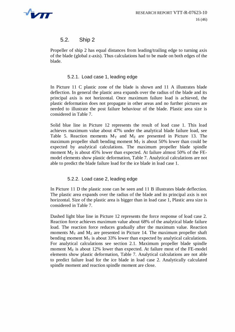
5.2. Ship 2
Propeller of ship 2 has equal distances from leading/trailing edge to turning axisof the blade (global zaxis). Thus calculations had to be made on both edges of theblade.
5.2.1. Load case 1, leading edge
In Picture 11 C plastic zone of the blade is shown and 11 A illustrates bladedeflection. In general the plastic area expands over the radius of the blade and itsprincipal axis is not horizontal. Once maximum failure load is achieved, theplastic deformation does not propagate in other areas and no further pictures areneeded to illustrate the post failure behaviour of the blade. Plastic area size isconsidered in Table 7.
Solid blue line in Picture 12 represents the result of load case 1. This loadachieves maximum value about 47% under the analytical blade failure load, seeTable 5. Reaction moments MY and MZ are presented in Picture 13. Themaximum propeller shaft bending moment MY is about 50% lower than could beexpected by analytical calculations. The maximum propeller blade spindlemoment MZ is about 45% lower than expected. At failure almost 50% of the FEmodel elements show plastic deformation, Table 7. Analytical calculations are notable to predict the blade failure load for the ice blade in load case 1.
5.2.2. Load case 2, leading edge
In Picture 11 D the plastic zone can be seen and 11 B illustrates blade deflection.The plastic area expands over the radius of the blade and its principal axis is nothorizontal. Size of the plastic area is bigger than in load case 1, Plastic area size isconsidered in Table 7.
Dashed light blue line in Picture 12 represents the force response of load case 2.Reaction force achieves maximum value about 68% of the analytical blade failureload. The reaction force reduces gradually after the maximum value. Reactionmoments MY and MZ are presented in Picture 14. The maximum propeller shaftbending moment MY is about 33% lower than expected by analytical calculations.For analytical calculations see section 2.1. Maximum propeller blade spindlemoment MZ is about 12% lower than expected. At failure most of the FEmodelelements show plastic deformation, Table 7. Analytical calculations are not ableto predict failure load for the ice blade in load case 2. Analytically calculatedspindle moment and reaction spindle moment are close.

RESEARCH REPORT VTTR076231017 (46)
Table 7, Ship 2 Plastic area at failure
where:Plastic elem. = Number of plastic elements at failure load, plasticity limits [0.5%10%]Total elem. = Number of total elements in the FEmodelRFmax = Maximum reaction force in Picture 12RM = Maximum reaction moment in Picture 13 and Picture 14Fex = Blade failure load, Table 5MY = analytical moment, Table 5MZ = analytical moment, Table 5Fex = Blade failure load, Table 5
Blade,Load case
Plastic elem./total elem.
Plasticelements[%]
ForceRFmax / Fex
Force[%]
BendingRMY/ MY
Bending[%]
SpindleRMz/ Mz
Spindle[%]
Ice,Load case 1
105308/217883 48.3% 0.555/1.044 53.2% 0.39/0.77 50.6% 0.17/0.31 54.8%
Ice,Load case 2
143998/217883 66.0% 0.713/1.044 68.3% 0.55/0.82 67.1% 0.14/0.16 87.5%

RESEARCH REPORT VTTR076231018 (46)
LOAD CASE 1, Force at 2/3 spindel arm LOAD CASE 2, Force at 1/3 spindel arm
A: Deformation at failure, Umax=157mm B: Deformation at failure, Umax=202mm
C: Plastic strain at failure, Umax=157mm, Maxstrain =8.3%
D: plastic strain at failure Umax=202mm, Maxstrain =8.4%
Picture 11, Ship 2 propeller blade behaviour under loading
RESEARCH REPORT VTTR076231019 (46)
5.2.3. Ship 2 Plots
Picture 12, Ship 2 Total end tip displacement (U) Reaction force
Picture 13, Ship 2 Reaction moments

RESEARCH REPORT VTTR076231020 (46)
Picture 14, Ship 2, Reaction moments, load case 2
RESEARCH REPORT VTTR076231021 (46)
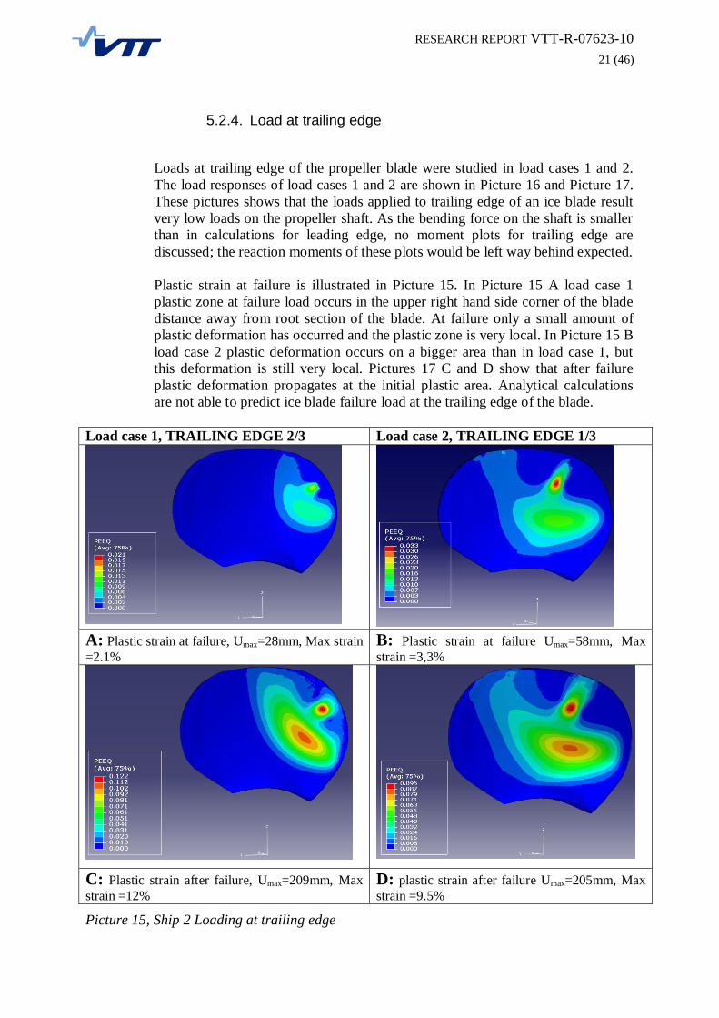
5.2.4. Load at trailing edge
Loads at trailing edge of the propeller blade were studied in load cases 1 and 2.The load responses of load cases 1 and 2 are shown in Picture 16 and Picture 17.These pictures shows that the loads applied to trailing edge of an ice blade resultvery low loads on the propeller shaft. As the bending force on the shaft is smallerthan in calculations for leading edge, no moment plots for trailing edge arediscussed; the reaction moments of these plots would be left way behind expected.
Plastic strain at failure is illustrated in Picture 15. In Picture 15 A load case 1plastic zone at failure load occurs in the upper right hand side corner of the bladedistance away from root section of the blade. At failure only a small amount ofplastic deformation has occurred and the plastic zone is very local. In Picture 15 Bload case 2 plastic deformation occurs on a bigger area than in load case 1, butthis deformation is still very local. Pictures 17 C and D show that after failureplastic deformation propagates at the initial plastic area. Analytical calculationsare not able to predict ice blade failure load at the trailing edge of the blade.
Load case 1, TRAILING EDGE 2/3 Load case 2, TRAILING EDGE 1/3
A: Plastic strain at failure, Umax=28mm, Max strain=2.1%
B: Plastic strain at failure Umax=58mm, Maxstrain =3,3%
C: Plastic strain after failure, Umax=209mm, Maxstrain =12%
D: plastic strain after failure Umax=205mm, Maxstrain =9.5%
Picture 15, Ship 2 Loading at trailing edge

RESEARCH REPORT VTTR076231022 (46)
5.2.5. Trailing edge, plots
Picture 16, Ship 2, Reaction at leading/trailing edge
Picture 17, Ship 2 Reaction at leading/trailing edge 1/3 spindle

RESEARCH REPORT VTTR076231023 (46)
5.2.6. Load case 3
As in the other load cases the plastic area due to bending was not found in the rootsection of the blade of ship 2 an additional load case was defined. A pressure isapplied on the area from R0.7 to R0.9, shown red in Picture 18. The plastic area inPicture 19 is at the root section of the blade and expands over the width of theblade. Force and moment reactions are shown in Picture 20 and Picture 21.Reaction forces and moments were compared to analytically calculated values inTable 8.
Obviously no significant spindle moment was generated, because the loading isuniformly distributed over the blade. Analytical calculations gave goodestimations to reaction moments and forces. The maximum reaction force andmoment both were about 7% lower than estimated.
Picture 18, Load case 3, Pressure onR0.7R0.9
Picture 19, Ship 2 plastic strain atfailure U=258mm, Load case 3
Table 8, Load case 3 failure values
Blade, Load case ForceRFmax / Fex
Force[%]
BendingRMY/ MY
Bending[%]
Ice, Load case 3 0.97/1.044 92.9% 0.77/0.83 92.7%
where:RFmax = Maximum reaction force in Picture 12RMY = Maximum reaction moment in Picture 20Fex = Blade failure load, Table 5MY = analytical moment, Table 5Fex = Blade failure load, Table 5

RESEARCH REPORT VTTR076231024 (46)
5.2.7. Load case 3, plots
Picture 20, Ship 2 ultimate failure force, Load case 3
Picture 21, Ship 2 Ultimate bending moment, Load case 3

RESEARCH REPORT VTTR076231025 (46)
5.3. Material property validation
In this final case the materials of the studied blades were changed so that ship 1was calculated with NiAlBronze and ship 2 was calculated with steel. All abovementioned load cases were calculated except ship 2 load at trailing edge. Naturallyblade failure loads by [1] were also calculated with respective materials, see Table10. Material properties are listed in Table 9 below.
Table 9, Material properties
Material Elastic ModulusE [GPa]
Yield/ Ultimatestrength [MPa]
Poisson constant Elongation[%]
NiAlBronze 123 235/650 0.33 19Steel 200 520/650 0.3 15
Table 10, Reference loads and moments, B
Blade, Load Case, Material ForceFex [MN]
BendingMY[MNm]
SpindleMZ[MNm]
Skew, Load case 1,NiAlBronze 1.44 2.18 0.84Skew, Load case 2,NiAlBronze 1.44 2.30 0.42Ice, Load case 1, Seel 1.52 1.12 0.45Ice, Load case 2, Seel 1.52 1.19 0.25Ice, Load case 3, Seel 1.52 1.21 0Where:Fex= blade failure load by [1], p.38 fomula 6.25MY= analytical propeller shaft bending moment with constant moment arm a, seePicture 4MZ= analytical spindle moment with constant moment arm 1/3B or 2/3B specifiedby load case, see Picture 4
RESEARCH REPORT VTTR076231026 (46)
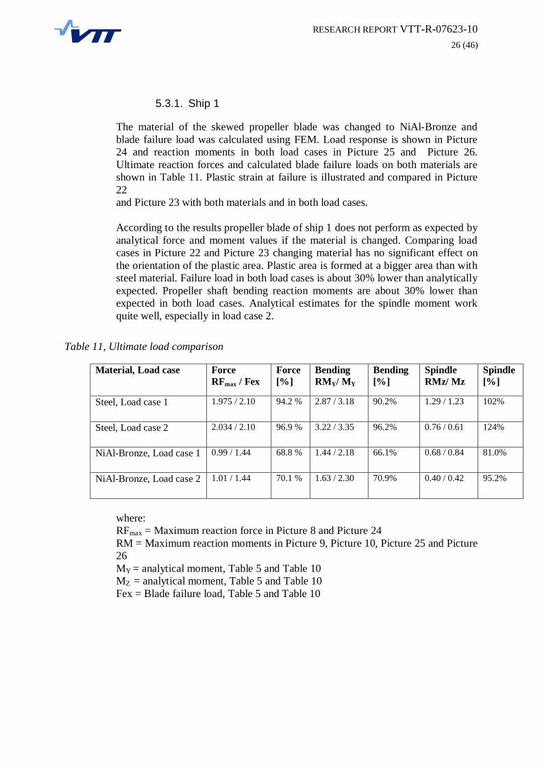
5.3.1. Ship 1
The material of the skewed propeller blade was changed to NiAlBronze andblade failure load was calculated using FEM. Load response is shown in Picture24 and reaction moments in both load cases in Picture 25 and Picture 26.Ultimate reaction forces and calculated blade failure loads on both materials areshown in Table 11. Plastic strain at failure is illustrated and compared in Picture22and Picture 23 with both materials and in both load cases.
According to the results propeller blade of ship 1 does not perform as expected byanalytical force and moment values if the material is changed. Comparing loadcases in Picture 22 and Picture 23 changing material has no significant effect onthe orientation of the plastic area. Plastic area is formed at a bigger area than withsteel material. Failure load in both load cases is about 30% lower than analyticallyexpected. Propeller shaft bending reaction moments are about 30% lower thanexpected in both load cases. Analytical estimates for the spindle moment workquite well, especially in load case 2.
Table 11, Ultimate load comparison
Material, Load case ForceRFmax / Fex
Force[%]
BendingRMY/ MY
Bending[%]
SpindleRMz/ Mz
Spindle[%]
Steel, Load case 1 1.975 / 2.10 94.2 % 2.87 / 3.18 90.2% 1.29 / 1.23 102%
Steel, Load case 2 2.034 / 2.10 96.9 % 3.22 / 3.35 96.2% 0.76 / 0.61 124%
NiAlBronze, Load case 1 0.99 / 1.44 68.8 % 1.44 / 2.18 66.1% 0.68 / 0.84 81.0%
NiAlBronze, Load case 2 1.01 / 1.44 70.1 % 1.63 / 2.30 70.9% 0.40 / 0.42 95.2%
where:RFmax = Maximum reaction force in Picture 8 and Picture 24RM = Maximum reaction moments in Picture 9, Picture 10, Picture 25 and Picture26MY = analytical moment, Table 5 and Table 10MZ = analytical moment, Table 5 and Table 10Fex = Blade failure load, Table 5 and Table 10

RESEARCH REPORT VTTR076231027 (46)
Ship 1, Load at 2/3 (NiAlBronze) Ship 1, Load at 2/3 (Steel)
A: Plastic strain at failure U=305mm B: Plastic strain after failure U=200mm
C: Plastic strain at failure U=305mm D: Plastic strain after failure U=400mm
Picture 22, Ship 1 Comparison of plastic deformation, Load case 1
RESEARCH REPORT VTTR076231028 (46)
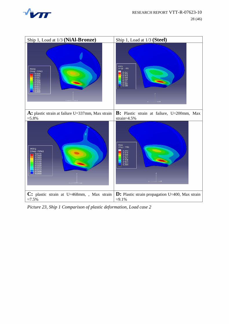
Ship 1, Load at 1/3 (NiAlBronze) Ship 1, Load at 1/3 (Steel)
A: plastic strain at failure U=337mm, Max strain5.8%
B: Plastic strain at failure, U 200mm, Maxstrain 4.5%
C: plastic strain at U=468mm, , Max strain7.5%
D: Plastic strain propagation U 400, Max strain9.1%
Picture 23, Ship 1 Comparison of plastic deformation, Load case 2

RESEARCH REPORT VTTR076231029 (46)
5.3.2. Ship 1, plots
Picture 24, Ship 1 Reaction force, NiAlBronze
Picture 25, Ship 1 Reaction moments, NiAlbronze

RESEARCH REPORT VTTR076231030 (46)
Picture 26, Ship 1, Reaction moments, Load case 2, NiAlBronze

RESEARCH REPORT VTTR076231031 (46)
5.3.3. Ship 2
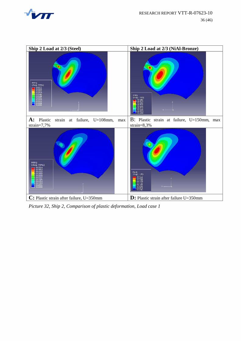
The material of ship 2 was changed form NiAlBronze to steel and blade failureload was calculated in three load cases using FEM. Response in load cases 1 and 2are shown in pictures 27 to 29 and load case 3 response is shown in Picture 30 andPicture 31. Plastic areas in load cases 1, 2 and 3 are examined in Picture 32 to 34.Maximum reaction forces and moments are compared to analytical values inTable 12.
1.1.1.1 Load cases 1 and 2
The blade failure load for steel in Picture 27 does not reach analytically calculatedvalue for both load cases. Failure in load case 1 occurs some 30% lower thananalytically expected and both reaction moment components do not reachexpected values. Plastic deformation is generated locally near the loaded area. Inload case 2 however analytical calculations give fairly good estimates for spindletorque and bending moment of the propeller shaft. Still plastic deformation occurslocally near the loaded area. Changing material has no significant effect on theorientation of the plastic area.
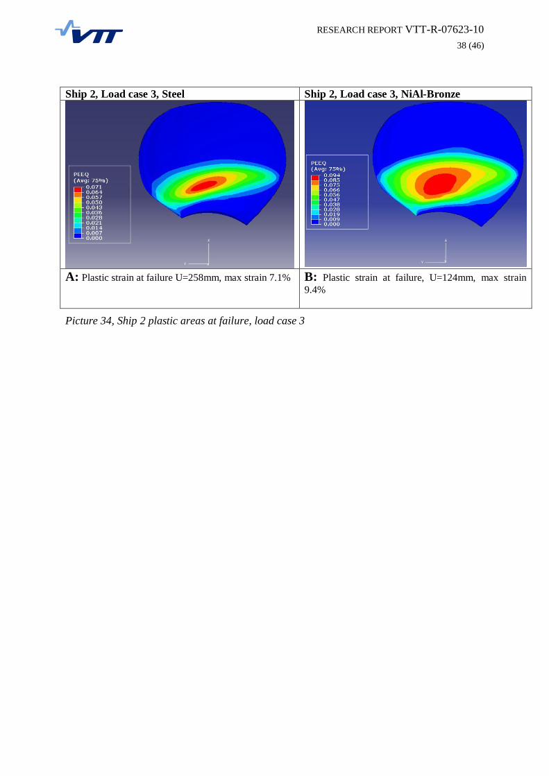
1.1.1.2 Load case 3Ultimate reaction force and bending moment values exceed the analyticalestimations by some 10 to 15%. Again spindle moment is not significantlygenerated. Plastic deformation is generated at the root of the blade and the areaexpands over the width of the blade.

RESEARCH REPORT VTTR076231032 (46)
Table 12, Ship 2, Ultimate load comparison
Material, Load case ForceRFmax/Fex
Force[%]
BendingRMY/ MY
Bending[%]
SpindleRMz/ Mz
Spindle[%]
NiAlBronze, Load case 1 0.555/1.044 53.2% 0.39/0.77 50.6% 0.17/0.31 54.8%
NiAlBronze, Load case 2 0.713/1.044 68.3% 0.55/0.82 67.1% 0.14/0.16 87.5%
NiAlBronze, Load case 3 0.97/1.044 92.9% 0.77/0.83 92.7% 0, notrelevant
Steel, Load case 1 1.05/1.52 69.1% 0.73/1.12 65.2% 0.32/0.45 71.1%
Steel, Load case 2 1.36/1.52 89.5% 1.04/1.19 87.4% 0.24/0.25 95.6%
Steel, Load case 3 1.75/1.52 115% 1.32/1.21 109% 0, notrelevant
where:RFmax = Maximum reaction force in Picture 8 and Picture 24RM = Maximum reaction moments in Picture 9, Picture 10, Picture 25 and Picture26MY = analytical moment, Table 5 and Table 10MZ = analytical moment, Table 5 and Table 10Fex = Blade failure load, Table 5 and Table 10

RESEARCH REPORT VTTR076231033 (46)
5.3.4. Ship 2, plots
Picture 27, Ship 2 Reaction forces, Steel
Picture 28, Ship2 Reaction moments, Steel

RESEARCH REPORT VTTR076231034 (46)
Picture 29, Ship 2 Reaction moments, Steel load case 2

RESEARCH REPORT VTTR076231035 (46)
Picture 30, Ship 2 force response, load case 3, Steel
Picture 31, Ship 2, reaction moment, load case 3, Steel
RESEARCH REPORT VTTR076231036 (46)
Ship 2 Load at 2/3 (Steel) Ship 2 Load at 2/3 (NiAlBronze)
A: Plastic strain at failure, U=108mm, maxstrain=7,7%
B: Plastic strain at failure, U=150mm, maxstrain=8,3%
C: Plastic strain after failure, U=350mm D: Plastic strain after failure U=350mm
Picture 32, Ship 2, Comparison of plastic deformation, Load case 1

RESEARCH REPORT VTTR076231037 (46)
Ship 2 Load at 1/3 (Steel) Ship 2 Load at 1/3 (NiAlBronze)
A: plastic strain at failure U=113mm, Max strain =6% B: plastic strain at failure Umax=202mm, Maxstrain =8.4%
C: plastic strain at U=348mm D: plastic strain at U=350mm
Picture 33, Ship 2, Comparison of plastic deformation, Load case 2
RESEARCH REPORT VTTR076231038 (46)
Ship 2, Load case 3, Steel Ship 2, Load case 3, NiAlBronze
A: Plastic strain at failure U=258mm, max strain 7.1% B: Plastic strain at failure, U=124mm, max strain9.4%
Picture 34, Ship 2 plastic areas at failure, load case 3

RESEARCH REPORT VTTR076231039 (46)
6. Conclusions
Ship1, Skew: Blade failure load estimation is realistic. No need to change the IceClass Regulations rule for blade failure load. If spindle arm would be changed to1/3, this would result in too low spindle torque estimates.
Ship 2, Ice blade: Blade failure load calculation does not work for blades of bigEAR (Expanded blade area ratio). The Ice Class Regulations rule for the bladefailure load assumes that the plastic hinge is formed at the blade root section.According to the numerical studies this assumption is not valid for this kind ofpropeller geometry thus leading to much smaller blade failure loads than theregulations predict.

RESEARCH REPORT VTTR076231040 (46)
7. Appendix
7.1. A: Calculation model validation
The geometry of the real propeller blades is too complex to be meshed with hexagonalelements, so the propellers are meshed with 10noded parabolic tetrahedron elements. Toconfirm the relevance of the blade FEmodels an element type validation was conducted.A test model is used to compare the results of different element types and to choose asufficient element density over the thickness of the plate.
The propeller blade is simplified to a plate model, seen in Picture 36. To makecalculations faster the plate was not fully modelled, instead three element layers broadmodel was made to represent the plate midsection, Picture 35. Dimensions of the testmodel are shown in Table 13. The thin model is restricted by boundary conditions tomatch the physical planestrain condition of the plate in pure bending. Isotropic steel wasused as material and strain hardening was modelled with a bilinear material model.
Table 13, Test model dimensions
model length (x) width (z) Plate thickness (y)Test model full scale 900mm 1200mm 100mmThin model 900mm 3mm 100mm
Picture 35, Thin test model Picture 36, Test model plate

RESEARCH REPORT VTTR076231041 (46)
1.1.2 Meshing, loading and boundary conditions
The test model was meshed with following element densities: i= 4, 6, 8, and16 elements over the thickness (y direction) of the plate. This element densityis marked with index i=”element density”. In the comparisons followingAbaqus element types were studied:
• Hexagonal C3D20, fully integrated, parabolic• Tetrahedron C3D10, fully integrated, parabolic
The C3D20 element represents the more accurate and well behaving element,which typically gives accurate results with less computational cost. The resultsof the tetrahedron C3D10 elements are compared to C3D20 results.
Loading was applied to the free end of the plate. The load was given as apressure of 24 MPa in the area seen in red in Picture 37. This area variesaccording to element size. The model was rigidly constrained at the rootsection, yellow cross seen in Picture 37.
Picture 37 illustrates the tetrahedron mesh of 8 elements over the thickness ofthe plate. After the first test run the plastic region due to bending wasdiscovered to appear in the region of the elements shown red in Picture 38.Data from the mentioned elements is discussed further in this report. The endtip displacement (U) is measured from the tip nodes at the free end of theplate.
The following quantities were compared:• Pressure load – displacement U• U Mises stress at Compression on surface• U plastic strain components at compression on the surface of the
plastic area• U plastic strain components at compression near neutral axis
Picture 37, Loaded area Picture 38, Elements at plastic region
RESEARCH REPORT VTTR076231042 (46)
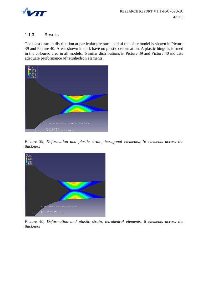
1.1.3 Results
The plastic strain distribution at particular pressure load of the plate model is shown in Picture39 and Picture 40. Areas shown in dark have no plastic deformation. A plastic hinge is formedin the coloured area in all models. Similar distributions in Picture 39 and Picture 40 indicateadequate performance of tetrahedron elements.
Picture 39, Deformation and plastic strain, hexagonal elements, 16 elements across thethickness
Picture 40, Deformation and plastic strain, tetrahedral elements, 8 elements across thethickness

RESEARCH REPORT VTTR076231043 (46)
The global response of the test models with the studied element densities is seen in Picture 41.Even i=4 model is able to describe the behaviour of the test model in bending and the yieldingpoint is realistic. Abaqus bilinear material model for steel is behaving well. The initial rapidrise of pressure load indicates loading in the elastic region of the material and yielding beginsat around 11 MPa pressure.
Picture 41, Global response
Von Mises stress at the surface of the plastic area is shown in Picture 42. Hex 16 modelperforms best and stress after yielding point is calculated correctly. All tetragonal modelsshoot over the yielding point, but this has no effect on the overall displacement response andthe problem might be solved by reducing the applied load increment.
Picture 42, Testmodel material behaviour

RESEARCH REPORT VTTR076231044 (46)
Plastic strain at the surface of the plastic region versus the plate tip displacement was verysimilar in all models. Picture 8 illustrates the behaviour of the plastic strain components at thecompression side of the plate at a distance of 25 mm from the surface. All models except thecoarse i=4 tetrahedron model converge to the result of hexagonal i=16.
Picture 43, Plastic behaviour
The overall plastic behaviour of the test models is compared in Table 14 below. At a specificload increment of 12MPa the amount of plastic elements is calculated. The tetrahedron modelwith four elements across the plate thickness predicts a larger plastic area than the othermodels due to the much bigger element size.
Table 14, Plastic elements
Test model No. of plastic elem./Total elem.
Plastic elements Pressure
Hex 16 1101/8793 12,5 % 12,02 MPaTet 8 2216/15320 14,5 % 12,00 MPaTet 6 1331/9374 14,2 % 12,00 MPaTet 4 686/4195 16,4 % 12,00 MPa

RESEARCH REPORT VTTR076231045 (46)
1.1.4 Conclusions
According to this study no less than 6 tetrahedron elements over the thickness of the propellerblade should be used to achieve an adequate resolution in the propeller blade failure loadanalysis. The real propeller models are meshed with 810 elements across the cross section inthe plastic region and its surroundings thus being able to predict the failure load reliably.

RESEARCH REPORT VTTR076231046 (46)
References
1. Finnish Maritime Administration Bulletin 10/10.12.2008, Ice Class Regulations 2008(FinnishSwedish Ice Class Rules), No. 2530/30/2008, ISSN 14559048


