
2/16/17 Electromagnetic Processes In Dispersive Media, Lecture 6 1
Polarized and unpolarised transverse waves, with applications to optical systems
T. Johnson

2/16/17 Electromagnetic Processes In Dispersive Media, Lecture 6 2
Outline
Previous lecture:• The quarter wave plate• Set up coordinate system suitable for transverse waves• Jones calculus; matrix formulation of how wave polarization changes
when passing through polarizing component– Examples: linear polarizer, quarter wave plate, Faraday rotation
This lecture• Statistical representation of incoherent/unpolarized waves
– Polarization tensors and Stokes vectors• The Poincaré sphere
• Muller calculus; matrix formulation for the transmission of partially polarized waves
2/16/17 Electromagnetic Processes In Dispersive Media, Lecture 6 3
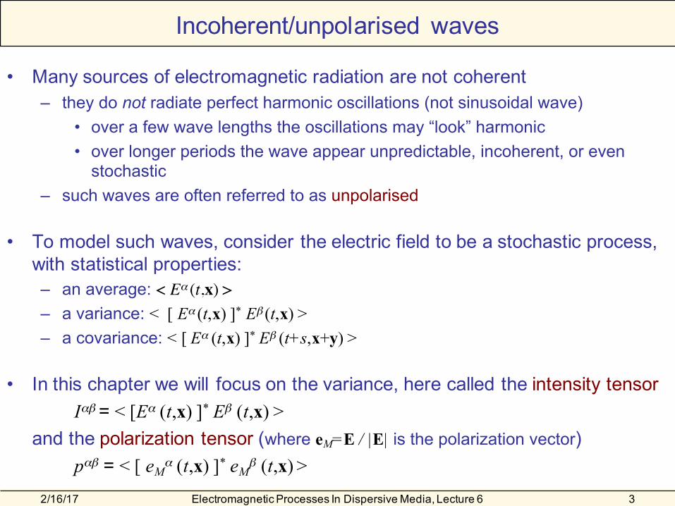
Incoherent/unpolarised waves
• Many sources of electromagnetic radiation are not coherent– they do not radiate perfect harmonic oscillations (not sinusoidal wave)
• over a few wave lengths the oscillations may “look” harmonic• over longer periods the wave appear unpredictable, incoherent, or even
stochastic– such waves are often referred to as unpolarised
• To model such waves, consider the electric field to be a stochastic process, with statistical properties:– an average: < Eα (t,x) >– a variance: < [ Eα (t,x) ]* Eβ (t,x) >– a covariance: < [ Eα (t,x) ]* Eβ (t+s,x+y) >
• In this chapter we will focus on the variance, here called the intensity tensorIαβ = < [Eα (t,x) ]* Eβ (t,x) >
and the polarization tensor (where eM=E / |E| is the polarization vector)pαβ = < [ eM
α (t,x) ]* eMβ (t,x) >

2/16/17 Electromagnetic Processes In Dispersive Media, Lecture 6 4
Representations for the polarization tensor
2/16/17 Electromagnetic Processes In Dispersive Media, Lecture 6 5
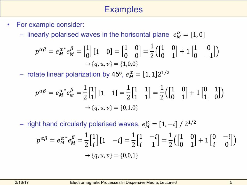
Examples
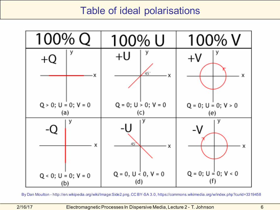
Table of ideal polarisations
By Dan Moulton - http://en.wikipedia.org/wiki/Image:Side2.png, CC BY-SA 3.0, https://commons.wikimedia.org/w/index.php?curid=3319458
2/16/17 Electromagnetic Processes In Dispersive Media, Lecture 2 - T. Johnson 6

2/16/17 Electromagnetic Processes In Dispersive Media, Lecture 6 7
The polarization tensor for unpolarized waves (1)
• What are the Stokes parameters for unpolarised waves?– Let the eM
1 and eM2 be stochastic variable
– The vector eM is normalised:– By symmetry (no statistical difference between eM
1 and eM2 )
– the polarization tensor then reads
– i.e. unpolarised have {q,u,v}={0,0,0}!
– Since eM1 and eM
2 are uncorrelated the offdiagonal term vanish
2/16/17 Electromagnetic Processes In Dispersive Media, Lecture 6 8
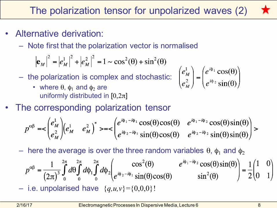
The polarization tensor for unpolarized waves (2)
• Alternative derivation:– Note first that the polarization vector is normalised
– the polarization is complex and stochastic:• where θ, φ1 and φ2 are
uniformly distributed in [0,2π]
• The corresponding polarization tensor
– here the average is over the three random variables θ, φ1 and φ2
– i.e. unpolarised have {q,u,v}={0,0,0}!
2/16/17 Electromagnetic Processes In Dispersive Media, Lecture 6 9
Poincaré sphere
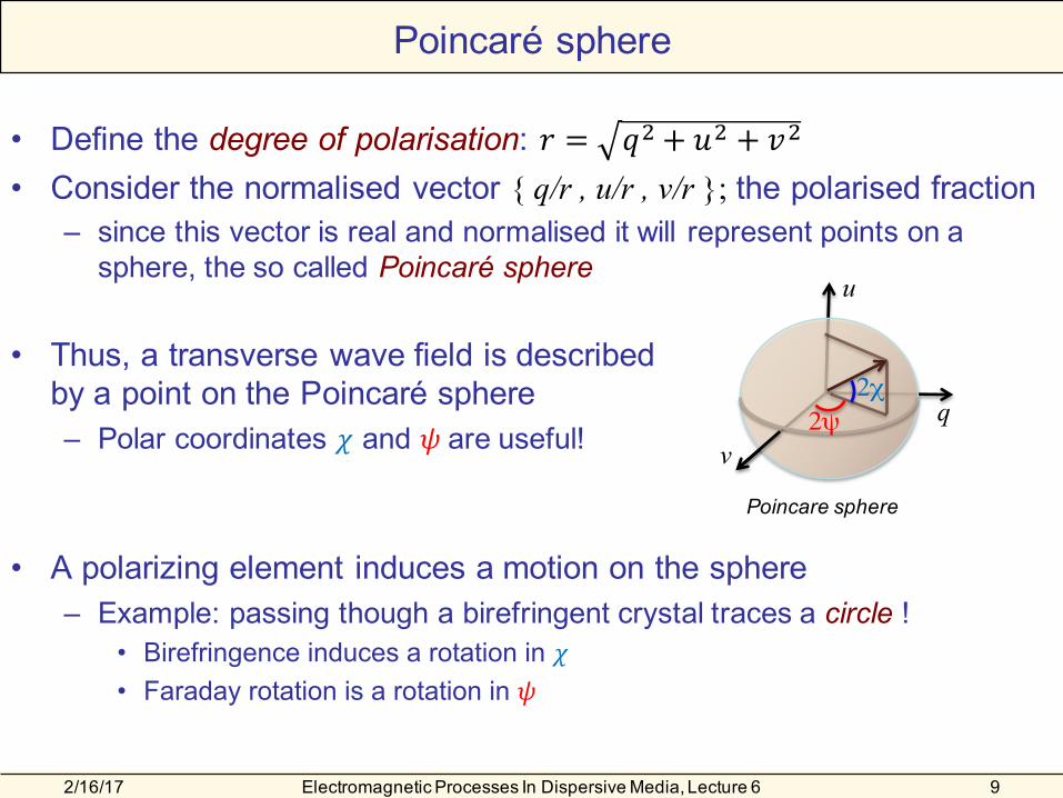
• Define the degree of polarisation: 𝑟 = 𝑞$ + 𝑢$ + 𝑣$
• Consider the normalised vector { q/r , u/r , v/r }; the polarised fraction– since this vector is real and normalised it will represent points on a
sphere, the so called Poincaré sphere
• Thus, a transverse wave field is described by a point on the Poincaré sphere– Polar coordinates 𝜒 and 𝜓 are useful!
• A polarizing element induces a motion on the sphere– Example: passing though a birefringent crystal traces a circle !
• Birefringence induces a rotation in 𝜒• Faraday rotation is a rotation in 𝜓
Poincare sphere
v
u
q2χ
2ψ

2/16/17 Electromagnetic Processes In Dispersive Media, Lecture 6 10
The Stokes vector
• Using unit- and Pauli-matrixes, we define τAαβ as:
• The intensity tensor, 𝐼+, = 𝐸+∗𝐸, , is also Hermitian:
𝐼+, =12 𝐼 1 0
0 1 + 𝑄 1 00 −1 + 𝑈 0 1
1 0 + 𝑉 0 −𝑖𝑖 0 = 𝐼 + 𝑄 𝑈 − 𝑖𝑉
𝑈 + 𝑖𝑉 𝐼 − 𝑄
– The four real parameters 𝐼,𝑄,𝑈, 𝑉 are the Stokes parameter– The Stokes vector is defined as 𝑆9 = 𝐼, 𝑄,𝑈,𝑉
• Using index notation the intensity tensor and the Stokes vector are related by:
– The matrixes τAαβ, defines a transformation between
Hermitian 2x2 matrixes and real 4-vectors

2/16/17 Electromagnetic Processes In Dispersive Media, Lecture 6 11
Outline
Previous lecture:• The quarter wave plate• Set up coordinate system suitable for transverse waves• Jones calculus; matrix formulation of how wave polarization changes
when passing through polarizing component– Examples: linear polarizer, quarter wave plate, Faraday rotation
This lecture• Statistical representation of incoherent/unpolarized waves
– Polarization tensors and Stokes vectors• The Poincare sphere
• Müller (Mueller) calculus; matrix formulation for the transmission of partially polarized waves– Example: Optical components– General theory for dispersive media

Müller matrixes• Müller matrixes maps incoming to outgoing Stokes vectors
𝑆9:;< = 𝑀9>𝑆>?@
• Since 𝑆9 is a four-vector, 𝑀9> is four-by-four• Müller matrixes generalises Jones matrixes by describing both
coherent and incoherent waves• How can we find the components of a Müller matrix, e.g. for a
linear polariser?a) 4x4=16 unknownb) Consider four experiments with different polarisation, e.g.
i. Horisontal polarisation, 𝑆 = 1,1,0,0ii. 45o tilted polarisation, 𝑆 = [1,0,1,0]iii. Circular polarisation, 𝑆 = [1,0,0,1]iv. Incoherent polarisation, 𝑆 = [1,0,0,0]
c) Calculate the relation 𝑆9:;<(𝑆>?@), for each of the four polarisations above.Note: This is four equations per polarisation, i.e. 16 equations!
2/16/17 Electromagnetic Processes In Dispersive Media, Lecture 2 - T. Johnson 12

2/16/17 Electromagnetic Processes In Dispersive Media, Lecture 6 13
Examples of Müller matrixes
Examples:
What is the Müller matrix for Faraday rotation?
Linear polarizer (Horizontal Transmission)
Linear polarizer (45o transmission)
Quarter wave plate(fast axis horizontal)
Attenuating filter (30% Transmission)

2/16/17 Electromagnetic Processes In Dispersive Media, Lecture 6 14
Examples of Müller matrixes
• Insert unpolarised light, SAin=[1,0,0,0]
– Step 1: Linear polariser transmit linearly polarised light
• In optics it is common to connect a series of optical elements• Consider a system with:
– a linear polarizer and – a quarter wave plate
– Step 2: Quarter wave plate transmit circularly polarised light
/ 2
2 x

• In weakly anisotropic media the wave equation can be rewritten on a form suitable for studying the wave polarisation.
– the left hand side can then be expanded to give
2/16/17 Electromagnetic Processes In Dispersive Media, Lecture 6 15
Weakly anisotropic media
• Write the weakly anisotropic transverse response as
– where ΔKαβ is a small perturbation
• The wave equation
– when ΔKij is a small, the 1st order dispersion relation reads: n2≈n02
small, <<1
2/16/17 Electromagnetic Processes In Dispersive Media, Lecture 6 16
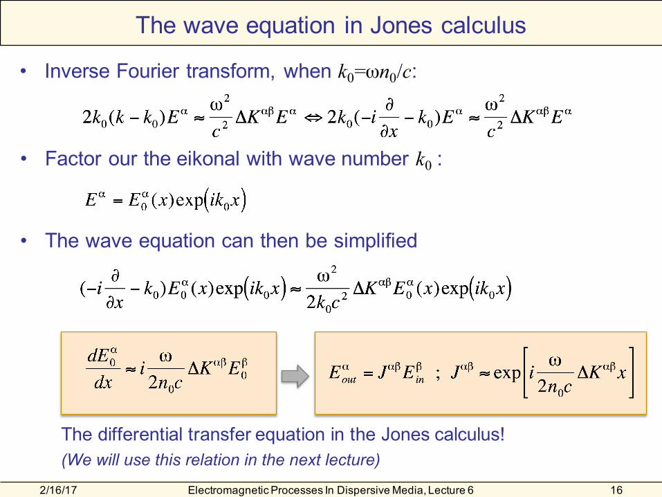
The wave equation in Jones calculus
• Inverse Fourier transform, when k0=ωn0/c:
• Factor our the eikonal with wave number k0 :
• The wave equation can then be simplified
The differential transfer equation in the Jones calculus!(We will use this relation in the next lecture)
2/16/17 Electromagnetic Processes In Dispersive Media, Lecture 6 17
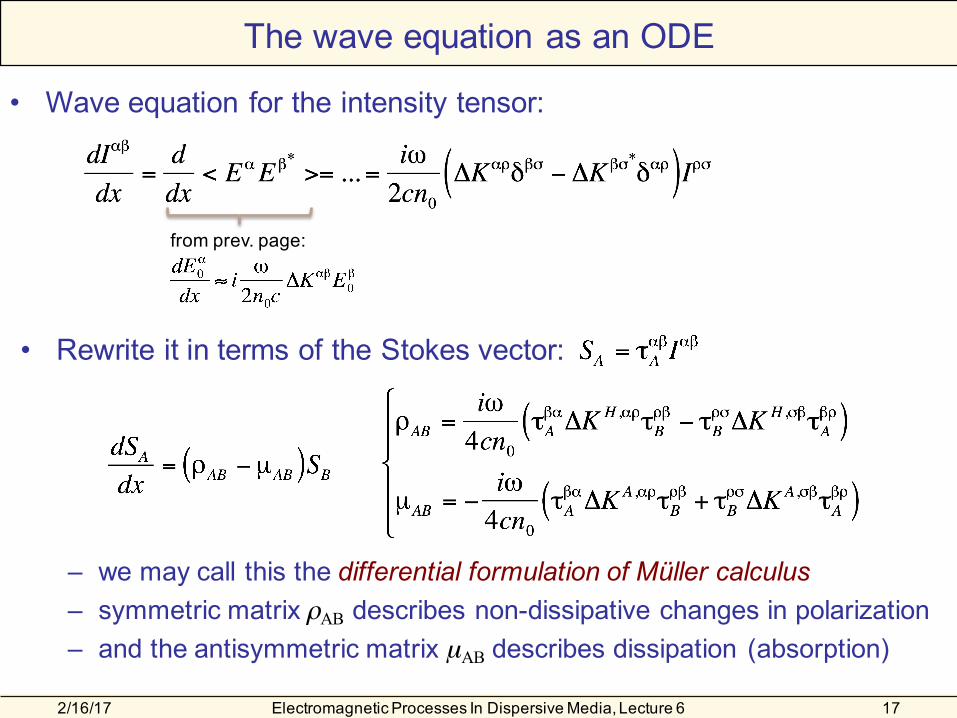
The wave equation as an ODE
• Rewrite it in terms of the Stokes vector:
• Wave equation for the intensity tensor:
– we may call this the differential formulation of Müller calculus– symmetric matrix ρAB describes non-dissipative changes in polarization– and the antisymmetric matrix µAB describes dissipation (absorption)
from prev. page:

2/16/17 Electromagnetic Processes In Dispersive Media, Lecture 6 18
The wave equation as an ODE
• The ODE for SA has the analytic solution (cmp to the ODE y’=ky)
– cmp with Taylor series for exponential
• Here MAB is a Müller matrix– MAB represents entire optical components / systems– This is a component based Müller calculus

Summary
• Unpolarised waves is incoherent when studied on time-scales longer than the wave-period.
• Representation of unpolarised waves using– Intensity tensor (Hermitian), 𝑝+,
– Polarisation tensor (Hermitian), 𝐼+,
– Stokes vector, 𝑆9, components of 𝐼+, using the Pauli matrixes as basis
• Polarised part of a wave field may be represented on the Poincarésphere
• Müller matrixes, 𝑀9>, describe changes in the polarisation when passing an optical component.
2/16/17 Electromagnetic Processes In Dispersive Media, Lecture 2 - T. Johnson 19


