

Portable High-Performance Programs
by
Matteo Frigo
Laurea, Universit`a di Padova (1992)Dottorato di Ricerca, Universit`a di Padova (1996)
Submitted to the Department of Electrical Engineering and Computer Sciencein partial fulfillment of the requirements for the degree of
Doctor of Philosophy
at the
MASSACHUSETTS INSTITUTE OF TECHNOLOGY
June 1999
© Matteo Frigo, MCMXCIX. All rights reserved.
The author hereby grants to MIT permission to reproduce and distribute publicly paperand electronic copies of this thesis document in whole or in part, and to grant others the
right to do so.
Author . . . . . . . . . . . . . . . . . . . . . . . . . . . . . . . . . . . . . . . . . . . . . . . . . . . . . . . . . . . . . . . . . . . . . . . . . . .Department of Electrical Engineering and Computer Science
June 23, 1999
Certified by . . . . . . . . . . . . . . . . . . . . . . . . . . . . . . . . . . . . . . . . . . . . . . . . . . . . . . . . . . . . . . . . . . . . . . .Charles E. Leiserson
Professor of Computer Science and EngineeringThesis Supervisor
Accepted by. . . . . . . . . . . . . . . . . . . . . . . . . . . . . . . . . . . . . . . . . . . . . . . . . . . . . . . . . . . . . . . . . . . . . .Arthur C. Smith
Chairman, Departmental Committee on Graduate Students

Copyright © 1999 Matteo Frigo.
Permission is granted to make and distribute verbatim copies of this thesis provided the copy-
right notice and this permission notice are preserved on all copies.
Permission is granted to copy and distribute modified versions of this thesis under the conditions
for verbatim copying, provided that the entire resulting derived work is distributed under the terms
of a permission notice identical to this one.
Permission is granted to copy and distribute translations of this thesis into another language,
under the above conditions for modified versions, except that this permission notice may be stated
in a translation approved by the Free Software Foundation.
2

Portable High-Performance Programs
by
Matteo Frigo
Submitted to the Department of Electrical Engineering and Computer Scienceon June 23, 1999, in partial fulfillment of the
requirements for the degree ofDoctor of Philosophy
Abstract
This dissertation discusses how to write computer programs that attain both high performance andportability, despite the fact that current computer systems have different degrees of parallelism, deepmemory hierarchies, and diverse processor architectures.
To cope with parallelism portably in high-performance programs, we present theCilk multi-threaded programming system. In the Cilk-5 system, parallel programs scale up to run efficientlyon multiple processors, but unlike existing parallel-programming environments, such as MPI andHPF, Cilk programs “scale down” to run on one processor as efficiently as a comparable C pro-gram. The typical cost of spawning a parallel thread in Cilk-5 is only between 2 and 6 times the costof a C function call. This efficient implementation was guided by thework-first principle, whichdictates that scheduling overheads should be borne by the critical path of the computation and notby the work. We show how the work-first principle inspired Cilk’s novel “two-clone” compilationstrategy and its Dijkstra-like mutual-exclusion protocol for implementing the ready deque in thework-stealing scheduler.
To cope portably with the memory hierarchy, we present asymptotically optimal algorithmsfor rectangular matrix transpose, FFT, and sorting on computers with multiple levels of caching.Unlike previous optimal algorithms, these algorithms arecache oblivious: no variables dependenton hardware parameters, such as cache size and cache-line length, need to be tuned to achieveoptimality. Nevertheless, these algorithms use an optimal amount of work and move data optimallyamong multiple levels of cache. For a cache with sizeZ and cache-line lengthL whereZ = (L2)the number of cache misses for anm� n matrix transpose is�(1 +mn=L). The number of cachemisses for either ann-point FFT or the sorting ofn numbers is�(1 + (n=L)(1 + logZ n)). Wealso give a�(mnp)-work algorithm to multiply anm � n matrix by ann � p matrix that incurs�(1 + (mn+ np+mp)=L+mnp=L
pZ) cache faults.
To attain portability in the face of both parallelism and the memory hierarchy at the same time,we examine thelocation consistencymemory model and theBACKER coherence algorithm formaintaining it. We prove good asymptotic bounds on the execution time of Cilk programs that uselocation-consistent shared memory.
To cope with the diversity of processor architectures, we develop the FFTW self-optimizingprogram, a portable C library that computes Fourier transforms. FFTW is unique in that it can au-tomatically tune itself to the underlying hardware in order to achieve high performance. Throughextensive benchmarking, FFTW has been shown to be typically faster than all other publicly avail-able FFT software, including codes such as Sun’s Performance Library and IBM’s ESSL that aretuned to a specific machine. Most of the performance-critical code of FFTW was generated auto-matically by a special-purpose compiler written in Objective Caml, which uses symbolic evaluationand other compiler techniques to produce “codelets”—optimized sequences of C code that can beassembled into “plans” to compute a Fourier transform. At runtime, FFTW measures the execution
3

time of many plans and uses dynamic programming to select the fastest. Finally, the plan drives aspecial interpreter that computes the actual transforms.
Thesis Supervisor: Charles E. LeisersonTitle: Professor of Computer Science and Engineering
4

Contents
1 Portable high performance 9
1.1 The scope of this dissertation . . . . . . . . . . . . . . . . . . . . . . . . . . . . . 9
1.1.1 Coping with parallelism . . . . . . . . . . . . . . . . . . . . . . . . . . . 9
1.1.2 Coping with the memory hierarchy . . . . . . . . . . . . . . . . . . . . . 11
1.1.3 Coping with parallelism and memory hierarchy together . . . . . . . . . . 13
1.1.4 Coping with the processor architecture . .. . . . . . . . . . . . . . . . . . 14
1.2 The methods of this dissertation. . . . . . . . . . . . . . . . . . . . . . . . . . . 16
1.3 Contributions . . .. . . . . . . . . . . . . . . . . . . . . . . . . . . . . . . . . . 17
2 Cilk 19
2.1 History of Cilk . . . . . . . . . . . . . . . . . . . . . . . . . . . . . . . . . . . . 21
2.2 The Cilk language .. . . . . . . . . . . . . . . . . . . . . . . . . . . . . . . . . . 22
2.3 The work-first principle . . . . . . . . . . . . . . . . . . . . . . . . . . . . . . . . 26
2.4 Example Cilk algorithms . .. . . . . . . . . . . . . . . . . . . . . . . . . . . . . 28
2.5 Cilk’s compilation strategy . . . . . . . . . . . . . . . . . . . . . . . . . . . . . . 31
2.6 Implementation of work-stealing . . . . . . . . . . . . . . . . . . . . . . . . . . . 36
2.7 Benchmarks . . . . . . . . . . . . . . . . . . . . . . . . . . . . . . . . . . . . . . 41
2.8 Related work . . . . . . . . . . . . . . . . . . . . . . . . . . . . . . . . . . . . . 43
2.9 Conclusion . . . . . . . . . . . . . . . . . . . . . . . . . . . . . . . . . . . . . . 44
3 Cache-oblivious algorithms 46
3.1 Matrix multiplication . . . . . . . . . . . . . . . . . . . . . . . . . . . . . . . . . 50
3.2 Matrix transposition and FFT. . . . . . . . . . . . . . . . . . . . . . . . . . . . . 52
3.3 Funnelsort . . . . . . . . . . . . . . . . . . . . . . . . . . . . . . . . . . . . . . 56
3.4 Distribution sort .. . . . . . . . . . . . . . . . . . . . . . . . . . . . . . . . . . 61
3.5 Other cache models. . . . . . . . . . . . . . . . . . . . . . . . . . . . . . . . . . 65
3.5.1 Two-level models . . . . . . . . . . . . . . . . . . . . . . . . . . . . . . . 65
3.5.2 Multilevel ideal caches. . . . . . . . . . . . . . . . . . . . . . . . . . . . 66
3.5.3 The SUMH model . . . . . . . . . . . . . . . . . . . . . . . . . . . . . . 67
5
3.6 Related work . . . . . . . . . . . . . . . . . . . . . . . . . . . . . . . . . . . . . 68
3.7 Conclusion . . . . . . . . . . . . . . . . . . . . . . . . . . . . . . . . . . . . . . 69
4 Portable parallel memory 71
4.1 Performance model and summary of results . . . . . . . . . . . . . . . . . . . . . 74
4.2 Location consistency and the BACKER coherence algorithm .. . . . . . . . . . . . 78
4.3 Analysis of execution time . . . . . . . . . . . . . . . . . . . . . . . . . . . . . . 79
4.4 Analysis of space utilization. . . . . . . . . . . . . . . . . . . . . . . . . . . . . 86
4.5 Related work . . . . . . . . . . . . . . . . . . . . . . . . . . . . . . . . . . . . . 92
4.6 Conclusion . . . . . . . . . . . . . . . . . . . . . . . . . . . . . . . . . . . . . . 93
5 A theory of memory models 94
5.1 Computation-centric memory models .. . . . . . . . . . . . . . . . . . . . . . . 96
5.2 Constructibility . . . . . . . . . . . . . . . . . . . . . . . . . . . . . . . . . . . . 99
5.3 Models based on topological sorts . . .. . . . . . . . . . . . . . . . . . . . . . . 102
5.4 Dag-consistent memory models . . . . . . . . . . . . . . . . . . . . . . . . . . . 104
5.5 Dag consistency and location consistency . . . . . . . . . . . . . . . . . . . . . . 108
5.6 Discussion . . . . . . . . . . . . . . . . . . . . . . . . . . . . . . . . . . . . . . . 109
6 FFTW 111
6.1 Background. . . . . . . . . . . . . . . . . . . . . . . . . . . . . . . . . . . . . . 114
6.2 Performance results . . . . . . . . . . . . . . . . . . . . . . . . . . . . . . . . . . 116
6.3 FFTW’s runtime structure . .. . . . . . . . . . . . . . . . . . . . . . . . . . . . . 127
6.4 The FFTW codelet generator. . . . . . . . . . . . . . . . . . . . . . . . . . . . . 133
6.5 Creation of the expression dag. . . . . . . . . . . . . . . . . . . . . . . . . . . . 137
6.6 The simplifier . . . . . . . . . . . . . . . . . . . . . . . . . . . . . . . . . . . . . 140
6.6.1 What the simplifier does . . . . . . . . . . . . . . . . . . . . . . . . . . . 140
6.6.2 Implementation of the simplifier . . . . . . . . . . . . . . . . . . . . . . . 143
6.7 The scheduler . . . . . . . . . . . . . . . . . . . . . . . . . . . . . . . . . . . . . 145
6.8 Real and multidimensional transforms .. . . . . . . . . . . . . . . . . . . . . . . 148
6.9 Pragmatic aspects of FFTW .. . . . . . . . . . . . . . . . . . . . . . . . . . . . . 150
6.10 Related work . . . . . . . . . . . . . . . . . . . . . . . . . . . . . . . . . . . . . 152
6.11 Conclusion . . . . . . . . . . . . . . . . . . . . . . . . . . . . . . . . . . . . . . 153
7 Conclusion 155
7.1 Future work . . . . . . . . . . . . . . . . . . . . . . . . . . . . . . . . . . . . . . 155
7.2 Summary . . . . . . . . . . . . . . . . . . . . . . . . . . . . . . . . . . . . . . . 158
6

Acknowledgements
This brief chapter is the most important of all. Computer programs will be outdated, and theorems
will be shown to be imprecise, incorrect, or just irrelevant, but the love and dedition of all people
who knowingly or unknowingly have contributed to this work is a lasting proof that life is supposed
to be beautiful and indeed it is.
Thanks to Charles Leiserson, my most recent advisor, for being a great teacher. He is always
around when you need him, and he always gets out of the way when you don’t. (Almost always,
that is. I wish he had not been around that day in Singapore when he convinced me to eat curried
fish heads.)
I remember the first day I met Gianfranco Bilardi, my first advisor. He was having trouble
with a computer, and he did not seem to understand how computers work. Later I learned that real
computers are the only thing Gianfranco has trouble with. In any other branch of human knowledge
he is perfectly comfortable.
Thanks to Arvind and Martin Rinard for serving on my thesis committee. Arvind and his student
Jan-Willem Maessen acquainted me with functional programming, and they had a strong influence
on my coding style and philosophy. Thanks to Toni Mian for first introducing me to Fourier trans-
forms. Thanks to Alan Edelman for teaching me numerical analysis and algorithms. Thanks to Guy
Steele and Gerry Sussman for writing the papers from which I learned what computer science is all
about.
It was a pleasure to develop Cilk together with Keith Randall, one of the most talented hackers
I have ever met. Thanks to Steven Johnson for sharing the burden of developing FFTW, and for
many joyful moments. Volker Strumpen influenced many of my current thoughts about computer
science as well as much of my personality. From him I learned a lot about computer systems.
Members of the Cilk group were a constant source of inspiration, hacks, and fun. Over the years, I
was honored to work with Bobby Blumofe, Guang-Ien Cheng, Don Dailey, Mingdong Feng, Chris
Joerg, Bradley Kuszmaul, Phil Lisiecki, Alberto Medina, Rob Miller, Aske Plaat, Harald Prokop,
Sridhar Ramachandran, Bin Song, Andrew Stark, and Yuli Zhou. Thanks to my officemates, Derek
Chiou and James Hoe, for many hours of helpful and enjoyable conversations.
Thanks to Tom Toffoli for hosting me in his house when I first arrived to Boston. Thanks to
7

Irena Sebeda for letting me into Tom’s house, because Tom was out of country that day. Thanks
for Benoit Dubertret for being my business partner in sharing a house and a keg of beer, and for the
good time we had during that partnership.
I wish to thanks all other people who made my stay in Boston enjoyable: Eric Chang, Nicole
Lazo, Victor Luchangco, Betty Pun, Stefano Soatto, Stefano Totaro, Joel Villa, Carmen Young.
Other people made my stay in Boston enjoyable even though they never came to Boston (proving
that computers are good for something): Luca Andreucci, Alberto Cammozzo, Enrico Giordani,
Gian Uberto Lauri, Roberto Totaro. Thanks to Andrea Pietracaprina and Geppino Pucci for helpful
discussions and suggestions at the beginning of my graduate studies.
Thanks to Giuseppe (Pino) Torresin and the whole staff of Biomedin for their help and support
during these five years, especially in difficult moments.
I am really grateful to Compaq for awarding me the Digital Equipment Corporation Fellowship.
Additional financial support was provided by the Defense Advanced Research Projects Agency
(DARPA) under Grants N00014-94-1-0985 and F30602-97-1-0270.
Many companies donated equipment that was used for the research described in this document.
Thanks to SUN Microsystems Inc. for its donation of a cluster of 9 8-processor Ultra HPC 5000
SMPs, which served as the primary platform for the development of Cilk and of earlier versions
of FFTW. Thanks to Compaq for donating a cluster of 7 4-processors AlphaServer 4100. Thanks
to Intel Corporation for donating a four-processor Pentium Pro machine, and thanks to the Linux
community for giving us a decent OS to run on it.
The Cilk and FFTW distributions use many tools from the GNU project, includingautomake,
texinfo, andlibtool developed by the Free Software Foundation. Thegenfft program was
written using Objective Caml, a small and elegant language developed by Xavier Leroy. This dis-
sertation was written on Linux using the TEX system by Donald E. Knuth, GNU Emacs, and various
other free tools such asgnuplot, perl, and thescm Scheme interpreter by Aubrey Jaffer.
Finally, my parents Adriano and Germana, and my siblings Marta and Enrico deserve special
thanks for their continous help and love. Now it’s time to go home and stay with them again.
I would have graduated much earlier had not Sandra taken care of me so well. She was patient
throughout this whole adventure.
8

Chapter 1
Portable high performance
This dissertation shows how to write computer programs whose performance is portable in the face
of multiprocessors, multilevel hierarchical memory, and diverseprocessor architectures.
1.1 The scope of this dissertation
Our investigation of portable high performance focuses on general-purpose shared memory multi-
processor machines with a memory hierarchy, which include uniprocessor PC’s and workstations,
symmetric multiprocessors (SMP’s), and CC-NUMA machines such as the SGI Origin 2000. We
are focusing on machines with shared memory because they are commonly available today and they
are growing in popularity because they offer good performance, low cost, and a single system image
that is easy to administer. Although we are focusing on shared-memory multiprocessor machines,
some of our techniques for portable high performance could be applied to other classes of machines
such as networks of workstations, vector computers, and DSP processors.
While superficially similar, shared-memory machines differ among each other in many ways.
The most obvious difference is the degree of parallelism (i.e., the number of processors). Fur-
thermore, platforms differ in the organization of the memory hierarchy and in their processor ar-
chitecture. In this dissertation we shall learn theoretical and empirical approaches to write high-
performance programs that are reasonably oblivious to variations in these parameters. These three
areas by no means exhaust the full topic of portability in high-performance systems, however. For
example, we are not addressing important topics such as portable performance in disk I/O, graphics,
user interfaces, and networking. We leave these topics to future research.
1.1.1 Coping with parallelism
As multiprocessors become commonplace, we ought to write parallel programs that run efficiently
both on single-processor and on multiprocessor platforms, so that a user can run a program to extract
9

maximum efficiency from whatever hardware is available, and a software developer does not need
to maintain both a serial and a parallel version of the same code. We ought to write these portable
parallel programs, but we don’t. Typically instead, a parallel program running on one processor is so
much slower and/or more complicated than the corresponding serial program that people prefer to
use two separate codes. The Cilk-5 multithreaded language, which I have designed and implemented
together with Charles Leiserson and Keith Randall [58], addresses this problem. In Cilk, one can
write parallel multithreaded programs that run efficiently on any number of processors, including 1,
and are in most cases not significantly more complicated than the corresponding serial codes.
Cilk is a simple extension of the C language with fork/join parallelism. Portability of Cilk pro-
grams derives from the observation, based on “Brent’s theorem” [32, 71], that any Cilk computation
can be characterized by two quantities: itswork T1, which is the total time needed to execute the
computation on one processor, and itscritical-path lengthT1, which is the execution time of the
computation on a computer with an infinite number of processors and a perfect scheduler (imag-
ine God’s computer). Work and critical-path are properties of the computation alone, and they do
not depend on the number of processors executing the computation. In previous work, Blumofe
and Leiserson [30, 25] designed Cilk’s “work-stealing” scheduler and proved that it executes a Cilk
program onP processors in timeTP , where
TP � T1=P +O(T1) : (1.1)
In this dissertation we improve on their work by observing that Equation (1.1) suggests both an
efficient implementation strategy for Cilk and an algorithmic design that only focuses on work and
critical path, as we shall now discuss.
In the current Cilk-5 implementation, a typical Cilk program running on a single processor is
only less than 5% slower than the corresponding sequential C program. To achieve this efficiency,
we aimed at optimizing the system for the common case, like much of the literature about compilers
[124] and computer architectures [79]. Rather than understanding quantitatively the common case,
mainly by studying the behavior of existing (and sometimes outdated) programs such as the SPEC
benchmarks, the common-case behavior of Cilk is predicted by a theoretical analysis that culminates
into thework-first principle. Specifically, overheads in the Cilk system can be divided into work
and critical-path overhead. The work-first principle states that Cilk incurs only work overhead in the
common case, and therefore we should put effort in reducing it even at the expense of critical-path
overhead. We shall derive the work-first principle from Equation (1.1) in Chapter 2, where we also
show how this principle inspired a “two-clone” compilation strategy for Cilk and a Dijkstra-like [46]
work-stealing protocol that does not use locks in the common case.
With an efficient implementation of Cilk and a performance model such as Equation (1.1),
we can now design portable high-performance multithreaded algorithms. Typically in Cilk, these
10

algorithms have adivide-and-conquerflavor. For example, the canonical Cilk matrix multiplication
program is recursive. To multiply 2 matrices of sizen�n, it splits each input matrix into 4 parts of
sizen=2�n=2, and it computes 8 matrix products recursively. (See Section 2.4.) In Cilk, even loops
are typically expressed as recursive procedures, because this strategy minimizes the critical path of
the program. To see why, consider a loop that increments every element of an arrayA of lengthn.
This program would be expressed in Cilk as a recursive procedure that incrementsA[0] if n = 1,
and otherwise calls itself recursively to increment the two halves ofA in parallel. This procedure
performs�(n) work, since the work of the recursion grows geometrically and is dominated by then
leaves, and the procedure has a�(lgn) critical path, because with an infinite number of processors
we reach the leaves of the recursion in time�(lgn), and all leaves can be computed in parallel.
The naive implementation that forksn threads in a loop, where each thread increments one array
element, is not as good in the Cilk model, because the last thread cannot be created until all previous
threads have been, yielding a critical path proportional ton.
Besides being high-performance, Cilk programs are also portable, because they do not depend
on the value ofP . Cilk shares this property with functional languages such as Multilisp [75], Mul-T
[94], Id [119], and data-parallel languages such as NESL [23], ZPL [34], and High Performance
Fortran [93, 80]. Among these languages, only NESL and ZPL feature an algorithmic performance
model like Cilk, and like Cilk, ZPL is efficient in practice [116]. The data-parallel style encouraged
by NESL and ZPL, however, can suffer large performance penalties because it introduces tempo-
rary arrays, which increase memory usage and pollute the cache. Compilers can eliminate these
temporaries with well-understood analyses [100], but the analysis is complicated and real compilers
are not always up to this task [116]. The divide-and-conquer approach of Cilk is immune from
these difficulties, and allows a more natural expression of irregular problems. We will see another
example of the importance of divide and conquer for portable high performance in Section 1.1.2
below.
1.1.2 Coping with the memory hierarchy
Modern computer systems are equipped with acache, or fast memory. Computers typically have
one or more levels of cache, which constitute thememory hierarchy, and any programming sys-
tem must deal with caches if it hopes to achieve high performance. To understand how to program
caches efficiently and portably, in this dissertation we explore the idea ofcache obliviousness. Al-
though a cache-oblivious algorithm does not “know” how big the cache is and how the cache is
partitioned into “cache lines,” these algorithms nevertheless use the cache asymptotically as effi-
ciently as their cache-aware counterparts. In Chapter 3 we shall see cache-oblivious algorithms for
matrix transpose and multiplication, FFT, and sorting. For problems such as sorting where lower
bounds on execution time and “cache complexity” are known, these cache-oblivious algorithms are
11

optimal in both respects.
A key idea for cache-oblivious algorithms is againdivide and conquer. To illustrate cache
obliviousness, consider again a divide and conquer matrix multiplication program that multiplies
two square matrices of sizen � n. Assume that initiallyn is big, so that the problem cannot
be solved fully within the cache, and therefore some traffic between the cache and the slow main
memory is necessary. The program partitions a problem of sizen into 8 subproblems of sizen=2
recursively, untiln = 1, in which case it computes the product directly. Even though the initial
array is too big to fit into cache, at some point during the recursionn reaches some valuen0 so
small that two matrices of sizen0�n0 can be multiplied fully within the cache. The program is not
aware of this transition and it continues the recursion down ton = 1, but the cache system is built
in such a way that it loads every element of then0 � n0 subarrays only once from main memory.
With the appropriate assumptions about the behavior of the cache, this algorithm can be proven to
use the cache asymptotically optimally, even though it does not depend on parameters such as the
size of the cache. (See Chapter 3.) An algorithm does not necessarily use the cache optimally just
because it is divide-and-conquer, of course, but in many cases the recursion can be designed so that
the algorithm is (asymptotically) optimal no matter how large the cache is.
How can I possibly advocate recursion instead of loops for high performance programs, given
that procedure calls are so expensive? I have two answers to this objection. First, procedure calls
are nottoo expensive, and the overhead of the recursion is amortized as soon as the leaves of the
recursion perform enough work. I have coded the procedure that adds 1 to every element of an
array using both a loop and a full recursion. The recursive program is about 8 times slower than
the loop on a 143-MHz UltraSPARC. If we unroll the leaves of the recursion so that each leaf
performs about 100 additions, the difference becomes less than 10%. To put things in perspective,
100 additions is roughly the work required to multiply two4 � 4 matrices or to perform a 16-
point Fourier transform. Second, we should keep in mind that current processors and compilers are
optimized for loop execution and not for recursion, and consequently procedure calls are relatively
more expensive than they could be if we designed systems explicitly to support efficient recursion.
Since divide and conquer is so advantageous for portable high-performance programs, we should
see this as a research opportunity to investigate architectural innovations and compiler techniques
that reduce the cost of procedure calls. For example, we need compilers that unroll recursion in the
same way current compilers unroll loops.
Cache-oblivious algorithms are designed for anideal cache, which is fully associative (objects
can reside anywhere in the cache) and features an optimal, omniscient replacement policy. In the
same way as a Cilk parallel algorithm is characterized by its work and critical-path length, a cache-
oblivious algorithm can be characterized by its workW and by itscache complexityQ(Z;L), which
measures the traffic between the cache and the main memory when the cache containsZ words and
it is partitioned into “lines” of lengthL. This theoretical framework allows algorithmic design for
12

the range(Z;L) of interest.
Our understanding of cache obliviousness is somewhat theoretical at this point, since today’s
computers do not feature ideal caches. Nevertheless, the ideal-cache assumptions are satisfied in
many cases. Consider for example the compilation of straight-line code with many (local) variables,
more than can fit into the register set of a processor. We can view the registers as the “cache” and
the rest of the memory as “main memory.” The compiler faces the problem of allocating variables
to registers so as to minimize the transfers between registers and memory, that is, the number of
“register spills” [115]. Because the whole sequences of accesses is known in advance, the compiler
can implement the optimal replacement strategy from [18], which replaces the register accessed
farthest in the future. Consequently, with a cache-oblivious algorithm and a good compiler, one can
write a single piece of C code that minimizes the traffic between registers and memory in such a
way that the same code is (asymptotically) optimal for any number of CPU registers. I have used
this idea in the FFTW “codelet generator” (see Chapter 6), which generates cache-oblivious fast
Fourier transform programs.
1.1.3 Coping with parallelism and memory hierarchy together
What happens when we parallelize a cache-oblivious algorithm with Cilk? The execution-time
upper bound from [25] (that is, Equation (1.1)) does not hold in the presence of caches, because the
proof does not account for the time spent in servicing cache misses. Furthermore, cache-oblivious
algorithms are not necessarily cache-optimal when they are executed in parallel, because of the
communication among caches.
In this dissertation, we combine the theories of Cilk and of cache obliviousness to provide a
performance bound similar to Equation (1.1) for Cilk programs that use hierarchical shared memory.
To prove this bound, we need to be precise about how we want memory to behave (the “memory
model”), and we must specify a protocol that maintains such a model. This dissertation presents a
memory model calledlocation consistencyand the BACKER coherence algorithm for maintaining
it. If B ACKER is used in conjunction with the Cilk scheduler, we derive a bound on the execution
time similar to Equation (1.1), but which takes the cache complexity into account. Specifically, we
prove that a Cilk program with workT1, critical pathT1, and cache complexityQ(Z;L) runs onP
processors in expected time
TP = O((T1 + �Q(Z;L))=P + �ZT1=L) ;
where� is the cost of transferring one cache line between main memory and the cache. As in
Equation (1.1), the first termT1 + �Q(Z;L) is the execution time on one processor when cache
effects are taken into account. The second term�ZT1=L accounts for the overheads of parallelism.
Informally, this term says that we might have to refill the cache from scratch from time to time,
13

where each refill costs time�Z=L, but this operation can happen at mostT1 times on average.
Although this model is simplistic, and it does not account for the fact that the service time is not
constant in practice (for example, on CC-NUMA machines), Cilk with BACKER is to my knowledge
the only system that provides performance bounds accounting for work, critical path, and cache
complexity.
Location consistency is defined within a novelcomputation-centricframework on memory
models. The implications of this framework are not directly relevant to the main point of this
dissertation, which is how to write portable fast programs, but I think that the computation-centric
framework is important from a “cultural” perspective, and therefore in Chapter 5 I have included a
condensed version of the computation-centric theory I have developed elsewhere [54].
1.1.4 Coping with the processor architecture
We personally like Brent's algorithm for univariate
minimization, as found on pages 79{80 of his
book \Algorithms for Minimization Without
Derivatives." It is pretty reliable and pretty
fast, but we cannot explain how it works.
(Gerald Jay Sussman)
While work, critical path, and cache complexity constitute a clean high-level algorithmic char-
acterization of programs, and while the Cilk theory is reasonably accurate in predicting the perfor-
mance of parallel programs, a multitude of real-life details are not captured by the simple theoretical
analysis of Cilk and of cache-oblivious algorithms. Currently we lack good models to analyze the
dependence of algorithms on the virtual memory system, the associativity of caches, the depth of a
processor pipeline, the number and the relative speeds of functional units within a processor, out-
of-order execution, branch predictors, not to mention busses, interlocks, prefetching instructions,
cache coherence, delayed branches, hazard detectors, traps and exceptions, and the aggressive code
transformations that compilers operate on programs. We shall refer to these parameters generically
as “processor architecture.” Even though compilers are essential to any high-performance system,
imagine for now that the compiler is part of some black box called “processor” that accepts our
program and produces the results we care about.
The behavior of “processors” these days can be quite amazing. If you experiment with your
favorite computer, you will discover that performance is not additive—that is, the execution time of
a program is not the sum of the execution time of its components—and it is not even monotonic.
For example, documented cases exist [95] where adding a “no-op” instruction to a program doubles
its speed, a phenomenon caused by the interaction of a short loop with a particular implementation
14
of branch prediction. As another example, the Pentium family of processors is much faster at
loading double precision floating-point numbers from memory if the address is a multiple of 8 (I
have observed a factor of 3 performance difference sometimes). Nevertheless, compilers likegcc
do not enforce this alignment because it would break binary compatibility with existing 80386
code, where the alignment was not important for performance. Consequently, your program might
become suddenly fast or slow when you add a local variable to a procedure. While it is unfortunate
that the system as a whole exhibits these behaviors, we cannot blame processors: The architectural
features that cause these anomalies are the very source of much of the processor performance. In
current processor architectures we gave away understandable designs to buy performance—a pact
with the devil [107] perhaps, but a good deal nonetheless.
Since we have no good model of processors, we cannot design “pipeline-oblivious” or “compiler-
oblivious” algorithms like we did for caches. Nevertheless, we can still write portable high-performance
programs if we adopt a “closed loop” approach. Our previous techniques were open-loop, and pro-
grams were by design oblivious to the number of processors and the cache. To cope with processors
architectures, we will write closed-loop programs capable of determining their own performance
and of adjusting their behavior to the complexity of the environment.
To explore this idea, I have developed aself-optimizing programthat can measure its own exe-
cution speed to adapt itself to the “processor.”FFTW is a comprehensive library of fast C routines
for computing thediscrete Fourier transform(DFT) in one or more dimensions, of both real and
complex data, and of arbitrary input size. FFTW automatically adapts itself to the machine it is run-
ning on so as to maximize performance, and it typically yields significantly better performance than
all other publicly available DFT software. More interestingly, while retaining complete portability,
FFTW is competitive with or faster than proprietary codes, such as Sun’s Performance Library and
IBM’s ESSL library, which are highly tuned for a single machine.
In order to adapt itself to the hardware, FFTW uses the property that the computation of a Fourier
transform can be decomposed into subproblems, and this decomposition can typically be accom-
plished in many ways. FFTW tries many different decompositions, itmeasurestheir execution time,
and it remembers the one that happens to run faster on a particular machine. FFTW does not attempt
to build a performance model and to predict the performance of a given decomposition, because all
my attempts to build a precise enough performance model to this end have failed. Instead, by mea-
suring its own execution time, FFTW approaches portability in a closed loop, end-to-end fashion,
and it compensates for our lack of understanding and for the imprecision of our theories.
FFTW’s portability is enabled by the extensive use ofmetaprogramming. About 95% of the
FFTW system is comprised ofcodelets, which are optimized sequences of C code that compute
subproblems of a Fourier transform. These codelets were generated automatically by aspecial-
purpose compiler, calledgenfft, which can only produce optimized Fourier transform programs,
but it excels at this task.genfft separates the logic of an algorithm from its implementation. The
15

user specifies an algorithm at a high level (the “program”), and also how he or she wants the code
to be implemented (the “metaprogram”). The advantage of metaprogramming is twofold. First,
genfft is necessary to produce a space of decompositions large enough for self-optimization to be
effective, since it would be impractical to write all codelets by hand. For example, the current FFTW
system comprises 120 codelets for a total of more than 56,000 lines of code. Only a few codelets are
used in typical situations, but it is important that all be available in order to be able to select the fast
ones. Second, the distinction between the program and the metaprogram allows for easy changes in
case we are desperate because every other portability technique fails. For example,genfft was at
one point modified to generate code for processors, such as the PowerPC [83], which feature a fused
multiply-add instruction. (This instruction computesa a + bc in one cycle.) This modification
required only 30 lines of code, and it improved the performance of FFTW on the PowerPC by 5-
10%, although it was subsequently disabled because it slowed down FFTW on other machines. This
example shows that machine-specific optimizations can be easily implemented if necessary. While
less desirable than a fully automatic system, changing 30 lines is still better than changing 56,000.
While recursive divide and conquer algorithms suffer from the overheads of procedure calls,
genfft helps overcoming the performance costs of the recursion. Codelets incur no recursion
overhead in the codelets, becausegenfft unrolls the recursion completely. The main FFTW self-
optimizing algorithm is also explicitly recursive, and it calls a codelet at the leaf of the recursion.
Since codelets perform a significant amount of work, however, the overhead of this recursion is
negligible. The FFTW system is described in Chapter 6.
This [other algorithm for univariate minimization]
is not so nice. It took 17 iterations [where Brent's
algorithm took 5] and we didn't get anywhere near
as good an answer as we got with Brent. On
the other hand, we understand how this works!
(Gerald Jay Sussman)
1.2 The methods of this dissertation
Our discussion of portable high performance draws ideas and methods from both the computer the-
ory and systems literatures. In some cases our discussion will be entirely theoretical, like for exam-
ple the asymptotic analysis of cache-oblivious algorithms. As is customary in theoretical analyses,
we assume an idealized model and we happily disregard constant factors. In other cases, we will
discuss at length implementation details whose only purpose is to save a handful CPU cycles. The
Cilk work-stealing protocol is an example of this systems approach. You should not be surprised if
we use these complementary sets of techniques, because the nature of the problem of portable high
16

performance demands both. Certainly, we cannot say that a technique is high-performance if it has
not been implemented, and therefore in this dissertation we pay attention to many implementation
details and to empirical performance results. On the other hand, we cannot say anything about the
portability of a technique unless we prove mathematically that the technique works on all machines.
Consequently, this dissertation oscillates between theory and practice, aiming at understanding sys-
tems and algorithms from both points of view whenever possible, and you should be prepared to
switch mind set from time to time.
1.3 Contributions
This dissertation shows how to write fast programs whose performance is portable. My main con-
tributions consist in two portable high-performance software systems, and in theoretical analyses of
portable high-performance algorithms and systems.
• The Cilk language and an efficient implementation of Cilk on SMP’s.Cilk provides simple
yet powerful constructs for expressing parallelism in an application. The language provides
the programmer with parallel semantics that are easy to understand and use. Cilk’s compila-
tion and runtime strategies, which are inspired by the “work-first principle,” are effective for
writing portable high-performance parallel programs.
• Cache-oblivious algorithmsprovide performance and portability across platforms with dif-
ferent cache sizes. They are oblivious to the parameters of the memory hierarchy, and yet
they use multiple levels of caches asymptotically optimally. This document presents cache-
oblivious algorithms for matrix transpose and multiplication, FFT, and sorting that are asymp-
totically as good as previously known cache-aware algorithms, and provably optimal for those
problems whose optimal cache complexity is known.
• The location consistency memory model and theBACKER coherence algorithmmarry Cilk
with cache-oblivious algorithms. This document proves good performance bounds for Cilk
programs that uses location consistency.
• The FFTW self-optimizing libraryimplements Fourier transforms of complex and real data
in one or more dimensions. While FFTW does not require machine-specific performance
tuning, its performance is comparable with or better than codes that were tuned for specific
machines.
The rest of this dissertation is organized as follows. Chapter 2 describes the work-first principle
and the implementation of Cilk-5. Chapter 3 defines cache obliviousness and gives cache-oblivious
17

algorithms for matrix transpose, multiplication, FFT, and sorting. Chapter 4 presents location con-
sistency and BACKER, and analyzes the performance of Cilk programs that use hierarchical shared
memory. Chapter 5 presents the computation-centric theory of memory models. Chapter 6 describes
the FFTW self-optimizing library andgenfft. Finally, Chapter 7 offers some concluding remarks.
18

Chapter 2
Cilk
This chapter describes theCilk system, which copes with parallelism in portable high-performance
programs. Portability in the context of parallelism is usually calledscalability: a program scales
if it attains good parallel speed-up. To really attain portable parallel high performance, however,
we must write parallel programs that both “scale up” and “scale down” to run efficiently on a
single processor—as efficiently as any sequential program that performs the same task. In this way,
users can exploit whatever hardware is available, and developers do not need to maintain separate
sequential and parallel versions of the same code.
Cilk is a multithreaded language for parallel programming that generalizes the semantics of C by
introducing simple linguistic constructs for parallel control. The Cilk language implemented by the
Cilk-5 release [38] uses the theoretically efficient scheduler from [25], but it was designed to scale
down as well as to scale up. Typically, a Cilk program runs on a single processor with less than 5%
slowdown relatively to a comparable C program. Cilk-5 is designed to run efficiently on contem-
porary symmetric multiprocessors (SMP’s), which provide hardware support for shared memory.
The Cilk group has coded many applications in Cilk, including the?Socrates and Cilkchess chess-
playing programs which have won prizes in international competitions. I was part of the team of
Cilk programmers which won First Prize, undefeated in all matches, in the ICFP’98 Programming
Contest sponsored by the 1998 International Conference on Functional Programming.1
Cilk’s constructs for parallelism are simple. Parallelism in Cilk is expressed with call/return
semantics, and the language has a simple “inlet” mechanism for nondeterministic control. The
philosophy behind Cilk development has been to make the Cilk language a true parallel extension
of C, both semantically and with respect to performance. On a parallel computer, Cilk control
constructs allow the program to execute in parallel. If the Cilk keywords for parallel control are
elided from a Cilk program, however, a syntactically and semantically correct C program results,
This chapter represents joint work with Charles Leiserson and Keith Randall. A preliminary version appears in [58].1Cilk is not a functional language, but the contest was open to entries in any programming language.
19

which we call theC elision (or more generally, theserial elision) of the Cilk program. Cilk is a
faithful extension of C, because the C elision of a Cilk program is a correct implementation of the
semantics of the program. On one processor, a parallel Cilk program scales down to run nearly as
fast as its C elision.
Unlike in Cilk-1 [29], where the Cilk scheduler was an identifiable piece of code, in Cilk-5
both the compiler and runtime system bear the responsibility for scheduling. To obtain efficiency,
we have, of course, attempted to reduce scheduling overheads. Some overheads have a larger im-
pact on execution time than others, however. The framework for identifying and optimizing the
common cases is provided by a theoretical understanding of Cilk’s scheduling algorithm [25, 30].
According to this abstract theory, the performance of a Cilk computation can be characterized by
two quantities: itswork, which is the total time needed to execute the computation serially, and its
critical-path length, which is its execution time on an infinite number of processors. (Cilk provides
instrumentation that allows a user to measure these two quantities.) Within Cilk’s scheduler, we can
identify a given cost as contributing to either work overhead or critical-path overhead. Much of the
efficiency of Cilk derives from the following principle, which will be justified in Section 2.3.
The work-first principle: Minimize the scheduling overhead borne by the work of a
computation. Specifically, move overheads out of the work and onto the critical path.
The work-first principle was used informally during the design of earlier Cilk systems, but Cilk-5
exploited the principle explicitly so as to achieve high performance. The work-first principle in-
spired a “two-clone” strategy for compiling Cilk programs. Thecilk2c compiler [111] is a type-
checking, source-to-source translator that transforms a Cilk source into a C postsource which makes
calls to Cilk’s runtime library. The C postsource is then run through thegcc compiler to produce
object code. Thecilk2c compiler produces two clones of every Cilk procedure—a “fast” clone
and a “slow” clone. The fast clone, which is identical in most respects to the C elision of the Cilk
program, executes in the common case where serial semantics suffice. The slow clone is executed
in the infrequent case when parallel semantics and its concomitant bookkeeping are required. All
communication due to scheduling occurs in the slow clone and contributes to critical-path overhead,
but not to work overhead.
The work-first principle also inspired a Dijkstra-like [46], shared-memory, mutual-exclusion
protocol as part of the runtime load-balancing scheduler. Cilk’s scheduler uses a “work-stealing”
algorithm in which idle processors, calledthieves, “steal” threads from busy processors, calledvic-
tims. Cilk’s scheduler guarantees that the cost of stealing contributes only to critical-path overhead,
and not to work overhead. Nevertheless, it is hard to avoid the mutual-exclusion costs incurred by a
potential victim, which contribute to work overhead. To minimize work overhead, instead of using
locking, Cilk’s runtime system uses a Dijkstra-like protocol (which we call theTHE) protocol, to
manage the runtime deque of ready threads in the work-stealing algorithm. An added advantage
20

of the THE protocol is that it allows an exception to be signaled to a working processor with no
additional work overhead, a feature used in Cilk’s abort mechanism.
Cilk features a provably efficient scheduler, but it cannot magically make sequential programs
parallel. To write portable parallel high performance, we must design scalable algorithms. In this
chapter, we will give simple examples of parallel divide-and-conquer Cilk algorithms for matrix
multiplication and sorting, and we will learn how to analyze work and critical-path length of Cilk
algorithms. The combination of these analytic techniques with the efficiency of the Cilk scheduler
allows us to write portable high-performance programs that cope with parallelism effectively.
The remainder of this chapter is organized as follows. Section 2.1 summarizes the develop-
ment history of Cilk. Section 2.2 overviews the basic features of the Cilk language. Section 2.3
justifies the work-first principle. Section 2.4 analyzes the work and critical-path length of example
Cilk algorithms. Section 2.5 describes how the two-clone strategy is implemented, and Section 2.6
presents the THE protocol. Section 2.7 gives empirical evidence that the Cilk-5 scheduler is effi-
cient. Section 2.8 presents related work.
2.1 History of Cilk
While the following sections describe Cilk-5 as it is today, it is important to start with a brief
summary of Cilk’s history, so that you can learn how the system evolved to its current state.
The original 1994 Cilk-1 release [25, 29, 85] featured the provably efficient, randomized, “work-
stealing” scheduler by Blumofe and Leiserson [25, 30]. The Cilk-1 language was clumsy and hard to
program, however, because parallelism was exposed “by hand” using explicit continuation passing.
Nonetheless, the?Socrates chess program was written in this language, and it placed 3rd in the 1994
International Computer Chess Championship running on NCSA’s 512-node CM5.
I became involved in the development of Cilk starting with Cilk-2. This system introduced
the same call/return semantics that Cilk-5 uses today. This innovation was made possible by the
outstanding work done by Rob Miller [111] on thecilk2c type-checking preprocessor. As the
name suggests,cilk2c translates Cilk into C, performing semantic and dataflow analysis in the
process. Most of Rob’scilk2c is still used in the current Cilk-5.
Cilk-3 added shared memory to Cilk. The innovation of Cilk-3 consisted in a novel mem-
ory model calleddag consistency[27, 26] and of the BACKER coherence algorithm to support it.
Cilk-3 was an evolutionary dead end as far as Cilk is concerned, because it implemented shared
memory in software using special keywords to denote shared variables, and both these techniques
disappeared from later versions of Cilk. The system was influential, however, in shaping the way
the Cilk authors thought about shared memory and multithreaded algorithms. Dag consistency
led to the computation-centric theory of memory models described in Chapter 5. The analysis of
dag-consistent algorithms of [26] led to the notion of cache obliviousness, which is described in
21

Chapter 3. Finally, the general algorithmic framework of Cilk and of cache-oblivious algorithms
provided a design model for FFTW (see Chapter 6).
While the first three Cilk systems were primarily developed on MPP’s such as the Thinking
Machines CM-5, the Cilk-4 system was targeted at symmetric multiprocessors. The system was
based on a novel “two-clone” compilation strategy (see Section 2.5 and [58]) that Keith Randall
invented. The Cilk language itself evolved to support “inlets” and nondeterministic programs. (See
Section 2.2.) Cilk-4 was designed at the beginning of 1996 and written in the spring. The new
implementation was made possible by a substantial and unexpected donation of SMP machines by
Sun Microsystems.
It soon became apparent, however, that the Cilk-4 system was too complicated, and in the Fall
of 1996 I decided to experiment with my own little Cilk system (initially called Milk, then Cilk-5).
Cilk-4 managed virtual memory explicitly in order to maintain the illusion of a cactus stack [113],
but this design decision turned out to be a mistake, because the need of maintaining a shared page ta-
ble complicated the implementation enormously, and memory mapping from user space is generally
slow in current operating systems.2 The new Cilk-5 runtime system was engineered from scratch
with simplicity as primary goal, and it used a simple heap-based memory manager. Thecilk2c
compiler did not change at all. While marginally slower than Cilk-4 on one processor, Cilk-5 turned
out to be faster on multiple processors because of simpler protocols and fewer interactions with the
operating system. In addition to this new runtime system, Cilk-5 featured a new debugging tool
called the “Nondeterminator” [52, 37], which finds data races in Cilk programs.
2.2 The Cilk language
This section presents a brief overview of the Cilk extensions to C as supported by Cilk-5. (For a
complete description, consult the Cilk-5 manual [38].) The key features of the language are the
specification of parallelism and synchronization, through thespawn andsync keywords, and the
specification of nondeterminism, usinginlet andabort.
The basic Cilk language can be understood from an example. Figure 2-1 shows a Cilk pro-
gram that computes thenth Fibonacci number.3 Observe that the program would be an ordinary C
program if the three keywordscilk, spawn, andsync were elided.
The keywordcilk identifiesfib as aCilk procedure, which is the parallel analog to a C
function. Parallelism is created when the keywordspawn precedes the invocation of a procedure.
The semantics of a spawn differs from a C function call only in that the parent can continue to
execute in parallel with the child, instead of waiting for the child to complete as is done in C. Cilk’s
2We could have avoid this mistake had we read Appel and Shao [13].3This program uses an inefficient algorithm which runs in exponential time. Although logarithmic-time methods are
known [42, p. 850], this program nevertheless provides a good didactic example.
22

#include <stdlib.h>
#include <stdio.h>
#include <cilk.h>
cilk int fib (int n)
{
if (n<2) return n;
else {
int x, y;
x = spawn fib (n-1);
y = spawn fib (n-2);
sync;
return (x+y);
}
}
cilk int main (int argc, char *argv[])
{
int n, result;
n = atoi(argv[1]);
result = spawn fib(n);
sync;
printf ("Result: %d\n", result);
return 0;
}
Figure 2-1: A simple Cilk program to compute thenth Fibonacci number in parallel (using a very badalgorithm).
scheduler takes the responsibility of scheduling the spawned procedures on the processors of the
parallel computer.
A Cilk procedure cannot safely use the values returned by its children until it executes async
statement. Thesync statement is a local “barrier,” not a global one as, for example, is used in
message-passing programming environments such as MPI [134]. In the Fibonacci example, async
statement is required before the statementreturn (x+y) to avoid the incorrect result that would
occur ifx andy are summed before they are computed. In addition to explicit synchronization pro-
vided by thesync statement, every Cilk procedure syncs implicitly before it returns, thus ensuring
that all of its children terminate before it does.
Cactus stack. Cilk extends the semantics of C by supporting cactus stack [78, 113, 137] semantics
for stack-allocated objects. From the point of view of a single Cilk procedure, a cactus stack behaves
much like an ordinary stack. The procedure can allocate and free memory by incrementing and
decrementing a stack pointer. The procedure views the stack as a linearly addressed space extending
23

A B C D E
A A
B
A
C
A
C
D
A
C
E
A
B C
D E
Figure 2-2: A cactus stack. The left-hand side shows a tree of procedures, where procedureA spawnsproceduresB andC, and procedureC spawns proceduresD andE. The right-hand side shows the stackview for the 5 procedures. For examples,D “sees” the frames of proceduresA andC, but not that ofB.
back from its own stack frame to the frame of its parent and continuing to more distant ancestors.
The stack becomes a cactus stack when multiple procedures execute in parallel, each with its own
view of the stack that corresponds to its call history, as shown in Figure 2-2.
Cactus-stack allocation mirrors the advantages of an ordinary procedure stack. Procedure-local
variables and arrays can be allocated and deallocated automatically by the runtime system in a
natural fashion. Separate branches of the cactus stack are insulated from each other, allowing two
threads to allocate and free objects independently, even though objects may be allocated with the
same address. Procedures can reference common data through the shared portion of their stack
address space.
Cactus stacks have many of the same limitations as ordinary procedure stacks [113]. For in-
stance, a child thread cannot return to its parent a pointer to an object that it has allocated. Similarly,
sibling procedures cannot share storage that they create on the stack. Just as with a procedure stack,
pointers to objects allocated on the cactus stack can only be safely passed to procedures below the
allocation point in the call tree. To alleviate these limitations, Cilk offers a heap allocator in the
style ofmalloc/free.
Inlets. Ordinarily, when a spawned procedure returns, the returned value is simply stored into a
variable in its parent’s frame:
x = spawn foo(y);
Occasionally, one would like to incorporate the returned value into the parent’s frame in a more
complex way. Cilk provides aninlet feature for this purpose, which was inspired in part by the inlet
feature of TAM [45].
24
cilk int fib (int n)
{
int x = 0;
inlet void summer (int result)
{
x += result;
return;
}
if (n<2) return n;
else {
summer(spawn fib (n-1));
summer(spawn fib (n-2));
sync;
return (x);
}
}
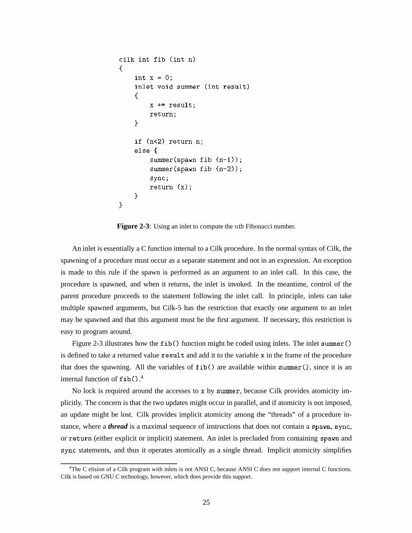
Figure 2-3: Using an inlet to compute thenth Fibonacci number.
An inlet is essentially a C function internal to a Cilk procedure. In the normal syntax of Cilk, the
spawning of a procedure must occur as a separate statement and not in an expression. An exception
is made to this rule if the spawn is performed as an argument to an inlet call. In this case, the
procedure is spawned, and when it returns, the inlet is invoked. In the meantime, control of the
parent procedure proceeds to the statement following the inlet call. In principle, inlets can take
multiple spawned arguments, but Cilk-5 has the restriction that exactly one argument to an inlet
may be spawned and that this argument must be the first argument. If necessary, this restriction is
easy to program around.
Figure 2-3 illustrates how thefib() function might be coded using inlets. The inletsummer()
is defined to take a returned valueresult and add it to the variablex in the frame of the procedure
that does the spawning. All the variables offib() are available withinsummer(), since it is an
internal function offib().4
No lock is required around the accesses tox by summer, because Cilk provides atomicity im-
plicitly. The concern is that the two updates might occur in parallel, and if atomicity is not imposed,
an update might be lost. Cilk provides implicit atomicity among the “threads” of a procedure in-
stance, where athread is a maximal sequence of instructions that does not contain aspawn, sync,
or return (either explicit or implicit) statement. An inlet is precluded from containingspawn and
sync statements, and thus it operates atomically as a single thread. Implicit atomicity simplifies
4The C elision of a Cilk program with inlets is not ANSI C, because ANSI C does not support internal C functions.Cilk is based on GNU C technology, however, which does provide this support.
25

reasoning about concurrency and nondeterminism without requiring locking, declaration of critical
regions, and the like.
Cilk provides syntactic sugar to produce certain commonly used inlets implicitly. For example,
the statementx += spawn fib(n-1) conceptually generates an inlet similar to the one in Figure 2-
3.
Abort. Sometimes, a procedure spawns off parallel work which it later discovers is unnecessary.
This “speculative” work can be aborted in Cilk using theabort primitive inside an inlet. A common
use ofabort occurs during a parallel search, where many possibilities are searched in parallel. As
soon as a solution is found by one of the searches, one wishes to abort any currently executing
searches as soon as possible so as not to waste processor resources. Theabort statement, when
executed inside an inlet, causes all of the already-spawned children of the procedure to terminate.
We considered using “futures” [76] with implicit synchronization, as well as synchronizing on
specific variables, instead of using the simplespawn andsync statements. We realized from the
work-first principle, however, that different synchronization mechanisms could have an impact only
on the critical-path of a computation, and so this issue was of secondary concern. Consequently,
we opted for implementation simplicity. Also, in systems that support relaxed memory-consistency
models, the explicitsync statement can be used to ensure that all side-effects from previously
spawned subprocedures have occurred.
In addition to the control synchronization provided bysync, Cilk programmers can use explicit
locking to synchronize accesses to data, providing mutual exclusion and atomicity. Data synchro-
nization is an overhead borne on the work, however, and although we have striven to minimize
these overheads, fine-grain locking on contemporary processors is expensive. We are currently in-
vestigating how to incorporate atomicity into the Cilk language so that protocol issues involved in
locking can be avoided at the user level. To aid in the debugging of Cilk programs that use locks,
the Cilk group has developed a tool called the “Nondeterminator” [37, 52], which detects common
synchronization bugs calleddata races.
2.3 The work-first principle
This section justifies the work-first principle stated at the beginning of this chapter by showing
that it follows from three assumptions. First, we assume that Cilk’s scheduler operates in practice
according to the theoretical analysis presented in [25, 30]. Second, we assume that in the common
case, ample “parallel slackness” [145] exists, that is, the parallelism of a Cilk program exceeds the
number of processors on which we run it by a sufficient margin. Third, we assume (as is indeed the
case) that every Cilk program has a C elision against which its one-processor performance can be
measured.
26

The theoretical analysis presented in [25, 30] cites two fundamental lower bounds as to how
fast a Cilk program can run. Let us denote byTP the execution time of a given computation on
P processors. The work of the computation is thenT1 and its critical-path length isT1. For a
computation withT1 work, the lower boundTP � T1=P must hold, because at mostP units of
work can be executed in a single step. In addition, the lower boundTP � T1 must hold, since a
finite number of processors cannot execute faster than an infinite number.5
Cilk’s randomized work-stealing scheduler [25, 30] executes a Cilk computation onP proces-
sors in expected time
TP = T1=P +O(T1) ; (2.1)
assuming an ideal parallel computer. This equation resembles “Brent’s theorem” [32, 71] and is
optimal to within a constant factor, sinceT1=P andT1 are both lower bounds. We call the first
term on the right-hand side of Equation (2.1) thework term and the second term thecritical-path
term. Importantly, all communication costs due to Cilk’s scheduler are borne by the critical-path
term, as are most of the other scheduling costs. To make these overheads explicit, we define the
critical-path overheadto be the smallest constantc1 such that
TP � T1=P + c1T1 : (2.2)
The second assumption needed to justify the work-first principle focuses on the “common-
case” regime in which a parallel program operates. Define theparallelism asP = T1=T1, which
corresponds to the maximum possible speedup that the application can obtain. Define also the
parallel slackness[145] to be the ratioP=P . Theassumption of parallel slacknessis thatP=P �c1, which means that the numberP of processors is much smaller than the parallelismP . Under
this assumption, it follows thatT1=P � c1T1, and hence from Inequality (2.2) thatTP � T1=P ,
and we obtain linear speedup. The critical-path overheadc1 has little effect on performance when
sufficient slackness exists, although it does determine how much slackness must exist to ensure
linear speedup.
Whether substantial slackness exists in common applications is a matter of opinion and empiri-
cism, but we suggest that slackness is the common case. The expressiveness of Cilk makes it easy to
code applications with large amounts of parallelism. For modest-sized problems, many applications
exhibit a parallelism of over 200, yielding substantial slackness on contemporary SMP’s. Even on
Sandia National Laboratory’s Intel Paragon, which contains 1824 nodes, the?Socrates chess pro-
gram (coded in Cilk-1) ran in its linear-speedup regime during the 1995 ICCA World Computer
5This abstract model of execution time ignores real-life details, such as memory-hierarchy effects, but is nonethelessquite accurate [29].
27

Chess Championship (where it placed second in a field of 24). Section 2.7 describes a dozen other
diverse applications which were run on an 8-processor SMP with considerable parallel slackness.
The parallelism of these applications increases with problem size, thereby ensuring they will be
portable to large machines.
The third assumption behind the work-first principle is that every Cilk program has a C elision
against which its one-processor performance can be measured. Let us denote byTS the running time
of the C elision. Then, we define thework overheadby c1 = T1=TS. Incorporating critical-path
and work overheads into Inequality (2.2) yields
TP � c1TS=P + c1T1 (2.3)
� c1TS=P ;
since we assume parallel slackness.
We can now restate the work-first principle precisely.Minimize c1, even at the expense of a
larger c1, becausec1 has a more direct impact on performance. Adopting the work-first principle
may adversely affect the ability of an application to scale up, however, if the critical-path overhead
c1 is too large. But, as we shall see in Section 2.7, critical-path overhead is reasonably small in
Cilk-5, and many applications can be coded with large amounts of parallelism.
The work-first principle pervades the Cilk-5 implementation. The work-stealing scheduler guar-
antees that with high probability, onlyO(PT1) steal (migration) attempts occur (that is,O(T1) on
average per processor), all costs for which are borne on the critical path. Consequently, the sched-
uler for Cilk-5 postpones as much of the scheduling cost as possible to when work is being stolen,
thereby removing it as a contributor to work overhead. This strategy of amortizing costs against
steal attempts permeates virtually every decision made in the design of the scheduler.
2.4 Example Cilk algorithms
In this section, we give example Cilk algorithms for matrix multiplication and sorting, and analyze
their work and critical-path length. The matrix multiplication algorithm multiplies twon � n ma-
trices using�(n3) work with critical-path length�(lg2 n). The sorting algorithm sorts an array of
n elements using work�(n lgn) with a critical-path length of�(lg3 n). The parallelism of these
algorithms is ample (P = �(n3= lg2 n) andP = �(n= lg2 n) respectively). Since Cilk executes a
program efficiently wheneverP � P , these algorithms are thus good candidates for portable high
performance. In this section, we focus on the theoretical analysis of these algorithms. We will see
in Section 2.7 that they also perform well in practice.
We start with thematrixmul matrix multiplication algorithm from [27]. To multiply then� nmatrixA by similar matrixB, matrixmul divides each matrix into fourn=2�n=2 submatrices and
28

uses the identity
"A11 A12
A21 A22
#�"B11 B12
B21 B22
#
=
"A11B11 A11B12
A21B11 A21B12
#+
"A12B21 A12B22
A22B21 A22B22
#:
The idea ofmatrixmul is to recursively compute the 8 products of the submatrices ofA andB
in parallel, and then add the subproducts together in pairs to form the result using recursive matrix
addition. In the base casen = 1, matrixmul computes the product directly.
Figure 2-4 shows Cilk code for an implementation ofmatrixmul that multiplies two square
matricesA andB yielding the output matrixR. The Cilk procedurematrixmul takes as arguments
pointers to the first block in each matrix as well as a variablen denoting the size of any row or
column of the matrices. Asmatrixmulexecutes, values are stored intoR, as well as into a temporary
matrixtmp.
Both the work and the critical-path length formatrixmul can be computed using recurrences.
The workT1(n) to multiplyn�nmatrices satisfies the recurrenceT1(n) = 8T1(n=2)+�(n2), since
addition of two matrices can be done usingO(n2) computational work, and thus,T1(n) = �(n3).
To derive a recurrence for the critical-path lengthT1(n), we observe that with an infinite number of
processors, only one of the 8 submultiplications is the bottleneck, because the 8 multiplications can
execute in parallel. Consequently, the critical-path lengthT1(n) satisfiesT1(n) = T1(n=2) +
�(lgn), because the parallel addition can be accomplished recursively with a critical path of length
�(lgn). The solution to this recurrence isT1(n) = �(lg2 n).
Algorithms exist for matrix multiplication with a shorter critical-path length. Specifically, two
n � n matrices can be multiplied using�(n3) work with a critical-path of�(lgn) [98], which is
shorter thanmatrixmul’s critical path. As we will see in Chapter 3, however, memory-hierarchy
considerations play a role in addition to work and critical path in the design of portable high-
performance algorithms. In Chapter 3 we will prove thatmatrixmul uses the memory hierarchy
efficiently, and in fact we will argue thatmatrixmul should be the preferred way to code even a
sequentialprogram.
We now discuss the Cilksort parallel sorting algorithm, which is a variant of ordinary mergesort.
Cilksort is inspired by [10]. Cilksort begins by dividing an array of elements into two halves, and
it sorts each half recursively in parallel. It then merges the two sorted halves back together, but in
a divide-and-conquer approach rather than with the usual serial merge. Say that we wish to merge
sorted arraysA andB. Without loss of generality, assume thatA is larger thanB. We begin by
dividing arrayA into two halves, lettingA1 denote the lower half andA2 the upper. We then take
the middle element ofA and use a binary search to discover where that element should fit into array
29

1 cilk void matrixmul(int n, float *A,
float *B,
float *R)
2 {
3 if (n == 1)
4 *R = *A * *B;
5 else {
6 float *A11,*A12,*A21,*A22,*B11,*B12,*B21,*B22;
7 float *A11B11,*A11B12,*A21B11,*A21B12,
*A12B21,*A12B22,*A22B21,*A22B22;
8 float tmp[n*n];
/* get pointers to input submatrices */
9 partition(n, A, &A11, &A12, &A21, &A22);
10 partition(n, B, &B11, &B12, &B21, &B22);
/* get pointers to result submatrices */
11 partition(n, R, &A11B11, &A11B12, &A21B11, &A21B12);
12 partition(n, tmp, &A12B21, &A12B22, &A22B21, &A22B22);
/* solve subproblems recursively */
13 spawn matrixmul(n/2, A11, B11, A11B11);
14 spawn matrixmul(n/2, A11, B12, A11B12);
15 spawn matrixmul(n/2, A21, B12, A21B12);
16 spawn matrixmul(n/2, A21, B11, A21B11);
17 spawn matrixmul(n/2, A12, B21, A12B21);
18 spawn matrixmul(n/2, A12, B22, A12B22);
19 spawn matrixmul(n/2, A22, B22, A22B22);
20 spawn matrixmul(n/2, A22, B21, A22B21);
21 sync;
/* add results together into R */
22 spawn matrixadd(n, tmp, R);
23 sync;
24 }
25 return;
26 }
Figure 2-4: Cilk code for recursive matrix multiplication.
30

B. This search yields a division of arrayB into subarraysB1 andB2. We then recursively merge
A1 with B1 andA2 with B2 in parallel and concatenate the results, which yields the desired fully
merged version ofA andB.
To analyze work and critical path of Cilksort, we first analyze the merge procedure. Letn be
the total size of the two arraysA andB. The merge algorithm splits a problem of sizen into
two problems of sizen1 andn2, wheren1 + n2 = n andmax fn1; n2g � (3=4)n, and it uses
O(lgn) work for the binary search. The work recurrence is thereforeT1(n) = T1(n1) + T1(n2) +
O(lgn), whose solution isT1(n) = �(n). The critical path recurrence is given byT1(n) =
T1(max fn1; n2g) + O(lgn), because the two subproblems can be solved in parallel but they
must both wait for the binary search to complete. Consequently, the critical path for merging is
T1(n) = �(lg2 n).
We now analyze Cilksort using the analysis of the merge procedure. Cilksort splits a problem of
sizen into two subproblems of sizen=2, and merges the results. The work recurrence isT1(n) =
2T1(n=2) + �(n), where�(n) work derives from the merge procedure. Similarly, the critical path
recurrence isT1(n) = T1(n=2) + �(lg2 n), where�(lg2 n) is the critical path of the merge step.
We conclude that Cilksort has work�(n lgn) and critical path�(lg3 n).
Cilksort is a simple algorithm that works well in practice. It uses optimal work, and its critical
path is reasonably short. As we will see in Section 2.7, Cilksort is only about 20% slower than
optimized sequential quicksort, and its parallelism is more than 1000 forn =4,100,000. Cilksort
thus qualifies as a portable high-performance parallel algorithm. A drawback of Cilksort is that
it does not use the memory hierarchy optimally. In Chapter 3 we will discuss more complicated
sorting algorithms that are optimal in this sense.
2.5 Cilk’s compilation strategy
This section describes how ourcilk2c compiler generates C postsource from a Cilk program. As
dictated by the work-first principle, our compiler and scheduler are designed to reduce the work
overhead as much as possible. Our strategy is to generate two clones of each procedure—afast
clone and aslowclone. The fast clone operates much as does the C elision and has little support for
parallelism. The slow clone has full support for parallelism, along with its concomitant overhead.
In the rest of this section, we first describe the Cilk scheduling algorithm. Then, we describe how
the compiler translates the Cilk language constructs into code for the fast and slow clones of each
procedure. Lastly, we describe how the runtime system links together the actions of the fast and
slow clones to produce a complete Cilk implementation. We can say, somewhat informally, that in
Cilk the fast clone takes care of high-performance, since it runs with minimal overhead, while the
slow clone takes care of portability, since it allows parallelism to be exploited.
As in lazy task creation [112], in Cilk-5 each processor (called aworker) maintains aready
31
deque(doubly-ended queue) of ready procedures (technically, procedure instances). Each deque
has two ends, aheadand atail, from which procedures can be added or removed. A worker operates
locally on the tail of its own deque, treating it much as C treats its call stack, pushing and popping
spawned activation frames. When a worker runs out of work, it becomes athief and attempts to
steal a procedure another worker, called itsvictim. The thief steals the procedure from the head of
the victim’s deque, the opposite end from which the victim is working.
When a procedure is spawned, the fast clone runs. Whenever a thief steals a procedure, however,
the procedure is converted into a slow clone. The Cilk scheduler guarantees that the number of
steals is small when sufficient slackness exists, and thus we expect the fast clones to be executed
most of the time. Thus, the work-first principle reduces to minimizing costs in the fast clone, which
contribute more heavily to work overhead. Minimizing costs in the slow clone, although a desirable
goal, is less important, since these costs contribute less heavily to work overhead and more to
critical-path overhead.
We minimize the costs of the fast clone by exploiting the structure of the Cilk scheduler. Because
we convert a procedure to its slow clone when it is stolen, we maintain the invariant that a fast clone
has never been stolen. Furthermore, none of the descendants of a fast clone have been stolen either,
since the strategy of stealing from the heads of ready deques guarantees that parents are stolen
before their children. As we will see, this simple fact allows many optimizations to be performed in
the fast clone.
We now describe how ourcilk2c compiler generates postsource C code for thefib procedure
from Figure 2-1. An example of the postsource for the fast clone offib is given in Figure 2-5. The
generated C code has the same general structure as the C elision, with a few additional statements.
In lines 4–5, anactivation frameis allocated forfib and initialized. The Cilk runtime system uses
activation frames to represent procedure instances. Using techniques similar to [72, 73], our inlined
allocator typically takes only a few cycles. The frame is initialized in line 5 by storing a pointer to
a static structure, called a signature, describingfib.
The first spawn infib is translated into lines 12–18. In lines 12–13, the state of thefib
procedure is saved into the activation frame. The saved state includes the program counter, encoded
as an entry number, and all live, dirty variables. Then, the frame is pushed on the runtime deque in
lines 14–15.6 Next, we call thefib routine as we would in C. Because thespawn statement itself
compiles directly to its C elision, the postsource can exploit the optimization capabilities of the C
compiler, including its ability to pass arguments and receive return values in registers rather than in
memory.
After fib returns, lines 17–18 check to see whether the parent procedure has been stolen. If
it has, we return immediately with a dummy value. Since all of the ancestors have been stolen as
6If the shared memory is not sequentially consistent, a memory fence must be inserted between lines 14 and 15 toensure that the surrounding writes are executed in the proper order.
32
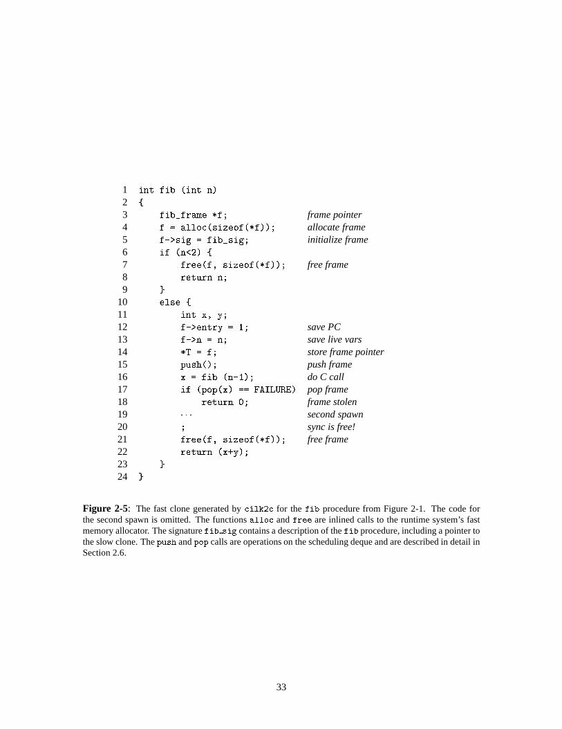
1 int fib (int n)
2 {
3 fib_frame *f; frame pointer4 f = alloc(sizeof(*f)); allocate frame5 f->sig = fib_sig; initialize frame6 if (n<2) {
7 free(f, sizeof(*f)); free frame8 return n;
9 }
10 else {
11 int x, y;
12 f->entry = 1; save PC13 f->n = n; save live vars14 *T = f; store frame pointer15 push(); push frame16 x = fib (n-1); do C call17 if (pop(x) == FAILURE) pop frame18 return 0; frame stolen19 � � � second spawn20 ; sync is free!21 free(f, sizeof(*f)); free frame22 return (x+y);
23 }
24 }
Figure 2-5: The fast clone generated bycilk2c for the fib procedure from Figure 2-1. The code forthe second spawn is omitted. The functionsalloc andfree are inlined calls to the runtime system’s fastmemory allocator. The signaturefib sig contains a description of thefib procedure, including a pointer tothe slow clone. Thepush andpop calls are operations on the scheduling deque and are described in detail inSection 2.6.
33

well, the C stack quickly unwinds and control is returned to the runtime system.7 The protocol to
check whether the parent procedure has been stolen is quite subtle—we postpone discussion of its
implementation to Section 2.6. If the parent procedure has not been stolen, it continues to execute
at line 19, performing the second spawn, which is not shown.
In the fast clone, allsync statements compile to no-ops. Because a fast clone never has any
children when it is executing, we know at compile time that all previously spawned procedures
have completed. Thus, no operations are required for async statement, as it always succeeds. For
example, line 20 in Figure 2-5, the translation of thesync statement is just the empty statement.
Finally, in lines 21–22,fib deallocates the activation frame and returns the computed result to its
parent procedure.
The slow clone is similar to the fast clone except that it provides support for parallel execution.
When a procedure is stolen, control has been suspended between two of the procedure’s threads,
that is, at a spawn or sync point. When the slow clone is resumed, it uses agoto statement to restore
the program counter, and then it restores local variable state from the activation frame. Aspawn
statement is translated in the slow clone just as in the fast clone. For async statement,cilk2c
inserts a call to the runtime system, which checks to see whether the procedure has any spawned
children that have not returned. Although the parallel bookkeeping in a slow clone is substantial, it
contributes little to work overhead, since slow clones are rarely executed.
The separation between fast clones and slow clones also allows us to compile inlets and abort
statements efficiently in the fast clone. An inlet call compiles as efficiently as an ordinary spawn.
For example, the code for the inlet call from Figure 2-3 compiles similarly to the following Cilk
code:
tmp = spawn fib(n-1);
summer(tmp);
Implicit inlet calls, such asx += spawn fib(n-1), compile directly to their C elisions. Anabort
statement compiles to a no-op just as async statement does, because while it is executing, a fast
clone has no children to abort.
The runtime system provides the glue between the fast and slow clones that makes the whole
system work. It includes protocols for stealing procedures, returning values between processors,
executing inlets, aborting computation subtrees, and the like. All of the costs of these protocols
can be amortized against the critical path, so their overhead does not significantly affect the running
time when sufficient parallel slackness exists. The portion of the stealing protocol executed by the
worker contributes to work overhead, however, thereby warranting a careful implementation. We
discuss this protocol in detail in Section 2.6.
7Thesetjmp/longjmp facility of C could have been used as well, but our unwinding strategy is simpler.
34

The work overhead of aspawn in Cilk-5 is only a few reads and writes in the fast clone—
3 reads and 5 writes for thefib example. We will experimentally quantify the work overhead
in Section 2.7. Some work overheads still remain in our implementation, however, including the
allocation and freeing of activation frames, saving state before a spawn, pushing and popping of the
frame on the deque, and checking if a procedure has been stolen. A portion of this work overhead
is due to the fact that Cilk-5 is duplicating the work the C compiler performs, but as Section 2.7
shows, this overhead is small. Although a production Cilk compiler might be able eliminate this
unnecessary work, it would likely compromise portability.
In Cilk-4, the precursor to Cilk-5, we took the work-first principle to the extreme. Cilk-4 per-
formed stack-based allocation of activation frames, since the work overhead of stack allocation is
smaller than the overhead of heap allocation. Because of the “cactus stack” [113] semantics of the
Cilk stack,8 however, Cilk-4 had to manage the virtual-memory map on each processor explicitly,
as was done in [137]. The work overhead in Cilk-4 for frame allocation was little more than that
of incrementing the stack pointer, but whenever the stack pointer overflowed a page, an expensive
user-level interrupt ensued, during which Cilk-4 would modify the memory map. Unfortunately,
the operating-system mechanisms supporting these operations were too slow and unpredictable,
and the possibility of a page fault in critical sections led to complicated protocols. Even though
these overheads could be charged to the critical-path term, in practice, they became so large that
the critical-path term contributed significantly to the running time, thereby violating the assump-
tion of parallel slackness. A one-processor execution of a program was indeed fast, but insufficient
slackness sometimes resulted in poor parallel performance.
In Cilk-5, we simplified the allocation of activation frames by simply using a heap. In the com-
mon case, a frame is allocated by removing it from a free list. Deallocation is performed by inserting
the frame into the free list. No user-level management of virtual memory is required, except for the
initial setup of shared memory. Heap allocation contributes only slightly more than stack allocation
to the work overhead, but it saves substantially on the critical path term. On the downside, heap allo-
cation can potentially waste more memory than stack allocation due to fragmentation. For a careful
analysis of the relative merits of stack and heap based allocation that supports heap allocation, see
the paper by Appel and Shao [13]. For an equally careful analysis that supports stack allocation, see
[110].
Thus, although the work-first principle gives a general understanding of where overheads should
be borne, our experience with Cilk-4 showed that large enough critical-path overheads can tip the
scales to the point where the assumptions underlying the principle no longer hold. We believe that
Cilk-5 work overhead is nearly as low as possible, given our goal of generating portable C output
8Suppose a procedure A spawns two children B and C. The two children can reference objects in A’s activation frame,but B and C do not see each other’s frame.
35

from our compiler.9 Other researchers have been able to reduce overheads even more, however, at
the expense of portability. For example, lazy threads [68] obtains efficiency at the expense of imple-
menting its own calling conventions, stack layouts, etc. Although we could in principle incorporate
such machine-dependent techniques into our compiler, we feel that Cilk-5 strikes a good balance be-
tween performance and portability. We also feel that the current overheads are sufficiently low that
other problems, notably minimizing overheads for data synchronization, deserve more attention.
2.6 Implementation of work-stealing
In this section, we describe Cilk-5’s work-stealing mechanism, which is based on a Dijkstra-like
[46], shared-memory, mutual-exclusion protocol called the “THE” protocol. In accordance with
the work-first principle, this protocol has been designed to minimize work overhead. For example,
on a 167-megahertz UltraSPARC I, thefib program with the THE protocol runs about 25% faster
than with hardware locking primitives. We first present a simplified version of the protocol. Then,
we discuss the actual implementation, which allows exceptions to be signaled with no additional
overhead.
Several straightforward mechanisms might be considered to implement a work-stealing proto-
col. For example, a thief might interrupt a worker and demand attention from this victim. This
strategy presents problems for two reasons. First, the mechanisms for signaling interrupts are slow,
and although an interrupt would be borne on the critical path, its large cost could threaten the as-
sumption of parallel slackness. Second, the worker would necessarily incur some overhead on the
work term to ensure that it could be safely interrupted in a critical section. As an alternative to
sending interrupts, thieves could post steal requests, and workers could periodically poll for them.
Once again, however, a cost accrues to the work overhead, this time for polling. Techniques are
known that can limit the overhead of polling [50], but they require the support of a sophisticated
compiler.
The work-first principle suggests that it is reasonable to put substantial effort into minimiz-
ing work overhead in the work-stealing protocol. Since Cilk-5 is designed for shared-memory
machines, we chose to implement work-stealing through shared-memory, rather than with message-
passing, as might otherwise be appropriate for a distributed-memory implementation. In our im-
plementation, both victim and thief operate directly through shared memory on the victim’s ready
deque. The crucial issue is how to resolve the race condition that arises when a thief tries to steal
the same frame that its victim is attempting to pop. One simple solution is to add a lock to the
deque using relatively heavyweight hardware primitives like Compare-And-Swap or Test-And-Set.
Whenever a thief or worker wishes to remove a frame from the deque, it first grabs the lock. This
9Although the runtime system requires some effort to port between architectures, the compiler requires no changeswhatsoever for different platforms.
36

solution has the same fundamental problem as the interrupt and polling mechanisms just described,
however. Whenever a worker pops a frame, it pays the heavy price to grab a lock, which contributes
to work overhead.
Consequently, we adopted a solution that employs Dijkstra’s protocol for mutual exclusion [46],
which assumes only that reads and writes are atomic. Because our protocol uses three atomic shared
variablesT, H, andE, we call it theTHE protocol. The key idea is that actions by the worker on
the tail of the queue contribute to work overhead, while actions by thieves on the head of the queue
contribute only to critical-path overhead. Therefore, in accordance with the work-first principle, we
attempt to move costs from the worker to the thief. To arbitrate among different thieves attempting to
steal from the same victim, we use a hardware lock, since this overhead can be amortized against the
critical path. To resolve conflicts between a worker and the sole thief holding the lock, however, we
use a lightweight Dijkstra-like protocol which contributes minimally to work overhead. A worker
resorts to a heavyweight hardware lock only when it encounters an actual conflict with a thief, in
which case we can charge the overhead that the victim incurs to the critical path.
In the rest of this section, we describe the THE protocol in detail. We first present a simplified
protocol that uses only two shared variablesT andH designating the tail and the head of the deque,
respectively. Later, we extend the protocol with a third variableE that allows exceptions to be
signaled to a worker. The exception mechanism is used to implement Cilk’sabort statement.
Interestingly, this extension does not introduce any additional work overhead.
The pseudocode of the simplified THE protocol is shown in Figure 2-6. Assume that shared
memory is sequentially consistent [96].10 The code assumes that the ready deque is implemented
as an array of frames. The head and tail of the deque are determined by two indicesT andH, which
are stored in shared memory and are visible to all processors. The indexT points to the first unused
element in the array, andH points to the first frame on the deque. Indices grow from the head
towards the tail so that under normal conditions, we haveT � H. Moreover, each deque has a lockL
implemented with atomic hardware primitives or with OS calls.
The worker uses the deque as a stack. (See Section 2.5.) Before aspawn, it pushes a frame onto
the tail of the deque. After aspawn, it pops the frame, unless the frame has been stolen. A thief
attempts to steal the frame at the head of the deque. Only one thief at the time may steal from the
deque, since a thief grabsL as its first action. As can be seen from the code, the worker altersT but
notH, whereas the thief only incrementsH and does not alterT.
The only possible interaction between a thief and its victim occurs when the thief is increment-
ing H while the victim is decrementingT. Consequently, it is always safe for a worker to append
a new frame at the end of the deque (push) without worrying about the actions of the thief. For a
10If the shared memory is not sequentially consistent, a memory fence must be inserted between lines 5 and 6 of theworker/victim code and between lines 3 and 4 of the thief code to ensure that these instructions are executed in the properorder.
37

Worker/Victim1 push() {
2 T++;
3 }
4 pop() {
5 T--;
6 if (H > T) {
7 T++;
8 lock(L);
9 T--;
10 if (H > T) {
11 T++;
12 unlock(L);
13 return FAILURE;
14 }
15 unlock(L);
16 }
17 return SUCCESS;
18 }
Thief1 steal() {
2 lock(L);
3 H++;
4 if (H > T) {
5 H--;
6 unlock(L);
7 return FAILURE;
8 }
9 unlock(L);
10 return SUCCESS;
11 }
Figure 2-6: Pseudocode of a simplified version of the THE protocol. The left part of the figure shows theactions performed by the victim, and the right part shows the actions of the thief. None of the actions besidesreads and writes are assumed to be atomic. For example,T--; can be implemented astmp = T; tmp =
tmp - 1; T = tmp;.
pop operation, there are three cases, which are shown in Figure 2-7. In case (a), the thief and the
victim can both obtain a frame from the deque. In case (b), the deque contains only one frame. If
the victim decrementsT without interference from thieves, it gets the frame. Similarly, a thief can
steal the frame as long as its victim is not trying to obtain it. If both the thief and the victim try to
grab the frame, however, the protocol guarantees that at least one of them discovers thatH > T. If
the thief discovers thatH > T, it restoresH to its original value and retreats. If the victim discovers
thatH > T, it restoresT to its original value and restarts the protocol after having acquiredL. With L
acquired, no thief can steal from this deque so the victim can pop the frame without interference (if
the frame is still there). Finally, in case (c) the deque is empty. If a thief tries to steal, it will always
fail. If the victim tries to pop, the attempt fails and control returns to the Cilk runtime system. The
protocol cannot deadlock, because each process holds only one lock at a time.
We now argue that the THE protocol contributes little to the work overhead. Pushing a frame
involves no overhead beyond updatingT. In the common case where a worker can successfully
pop a frame, the pop protocol performs only 6 operations—2 memory loads, 1 memory store, 1
decrement, 1 comparison, and 1 (predictable) conditional branch. Moreover, in the common case
where no thief operates on the deque, bothH andT can be cached exclusively by the worker. The
expensive operation of a worker grabbing the lockL occurs only when a thief is simultaneously
38

1
2
3
4
5
6
(c)(b)(a)
H
T
H
T
H=T
Thief
Victim
Figure 2-7: The three cases of the ready deque in the simplified THE protocol. A dark entry indicates thepresence of a frame at a certain position in the deque. The head and the tail are marked byT andH.
trying to steal the frame being popped. Since the number of steal attempts depends onT1, not on
T1, the relatively heavy cost of a victim grabbingL can be considered as part of the critical-path
overheadc1 and does not influence the work overheadc1.
We ran some experiments to determine the relative performance of the THE protocol versus
the straightforward protocol in whichpop just locks the deque before accessing it. On a 200-
megahertz Pentium Pro running Linux andgcc 2.7.1, the THE protocol is only about 5% faster than
the locking protocol. This machine’s memory model requires that a memory fence instruction be
inserted between lines 5 and 6 of thepop pseudocode. On this processor, the THE protocol spends
about half of its time in the memory fence. On a 167-megahertz UltraSPARC I, however, the THE
protocol is about 25% faster than the simple locking protocol. In this case we tried to quantify the
performance impact of the memory fence (membar) instruction, too, but in all our experiments the
execution times of the code with and withoutmembar are about the same.
In addition to this performance advantage, because it replaces locks with memory synchroniza-
tion, the THE protocol is more “nonblocking” than a straightforward locking protocol. Conse-
quently, the THE protocol is less prone to problems that arise when spin locks are used extensively.
For example, even if a worker is suspended by the operating system during the execution ofpop, the
infrequency of locking in the THE protocol means that a thief can usually complete a steal operation
on the worker’s deque. Recent work by Arora et al. [14] has shown that a completely nonblocking
work-stealing scheduler can be implemented. Using these ideas, Lisiecki and Medina [101] have
39

Program Size T1 T1 P c1 T8 T1=T8 TS=T8fib 35 12.77 0.0005 25540 3.63 1.60 8.0 2.2blockedmul 1024 29.9 0.0044 6730 1.05 4.3 7.0 6.6notempmul 1024 29.7 0.015 1970 1.05 3.9 7.6 7.2strassen 1024 20.2 0.58 35 1.01 3.54 5.7 5.6
*cilksort 4; 100; 000 5.4 0.0049 1108 1.21 0.90 6.0 5.0yqueens 22 150. 0.0015 96898 0.99 18.8 8.0 8.0yknapsack 30 75.8 0.0014 54143 1.03 9.5 8.0 7.7lu 2048 155.8 0.42 370 1.02 20.3 7.7 7.5
*cholesky BCSSTK32 1427. 3.4 420 1.25 208. 6.9 5.5heat 4096 � 512 62.3 0.16 384 1.08 9.4 6.6 6.1fft 220 4.3 0.0020 2145 0.93 0.77 5.6 6.0barnes-hut 216 124. 0.15 853 1.02 16.5 7.5 7.4
Figure 2-8: The performance of example Cilk programs. Times are in seconds and are accurate to withinabout 10%. The serial programs are C elisions of the Cilk programs, except for those programs that arestarred (*), where the parallel program implements a different algorithm than the serial program. Programslabeled by a dagger (y) are nondeterministic, and thus, the running time on one processor is not the same asthe work performed by the computation. For these programs, the value forT1 indicates the actual work of thecomputation on 8 processors, and not the running time on one processor.
modified the Cilk-5 scheduler to make it completely nonblocking. Their experience is that the THE
protocol greatly simplifies a nonblocking implementation.
The simplified THE protocol can be extended to support the signaling of exceptions to a worker.
In Figure 2-6, the indexH plays two roles: it marks the head of the deque, and it marks the point
that the worker cannot cross when it pops. These places in the deque need not be the same. In
the full THE protocol, we separate the two functions ofH into two variables:H, which now only
marks the head of the deque, andE, which marks the point that the victim cannot cross. Whenever
E > T, some exceptional condition has occurred, which includes the frame being stolen, but it can
also be used for other exceptions. For example, settingE = 1 causes the worker to discover the
exception at its next pop. In the new protocol,E replacesH in line 6 of the worker/victim. Moreover,
lines 7–15 of the worker/victim are replaced by a call to anexception handlerto determine the
type of exception (stolen frame or otherwise) and the proper action to perform. The thief code is
also modified. Before trying to steal, the thief incrementsE. If there is nothing to steal, the thief
restoresE to the original value. Otherwise, the thief steals frameH and incrementsH. From the point
of view of a worker, the common case is the same as in the simplified protocol: it compares two
pointers (E andT rather thanH andT).
The exception mechanism is used to implementabort. When a Cilk procedure executes an
abort instruction, the runtime system serially walks the tree of outstanding descendants of that
procedure. It marks the descendants as aborted and signals an abort exception on any processor
working on a descendant. At its nextpop, an aborted procedure will discover the exception, notice
that it has been aborted, and return immediately. It is conceivable that a procedure could run for a
40

long time without executing apop and discovering that it has been aborted. We made the design
decision to accept the possibility of this unlikely scenario, figuring that more cycles were likely to
be lost in work overhead if we abandoned the THE protocol for a mechanism that solves this minor
problem.
2.7 Benchmarks
In this section, we evaluate the performance of Cilk-5. We show that on 12 applications, the work
overheadc1 is close to 1, which indicates that the Cilk-5 implementation exploits the work-first
principle effectively and achieves the goal of “scaling down” to 1 processor. We then present a
breakdown of Cilk’s work overheadc1 on four machines. Finally, we present experiments showing
that Cilk applications “scale up” as well, and that the critical-path overheadc1 is reasonably small.
Our experiments show that Cilk delivers both high performance and portability, at least on the SMP
machines targeted by the Cilk-5 implementation.
Figure 2-8 shows a table of performance measurements taken for 12 Cilk programs on a Sun
Enterprise 5000 SMP with 8 167-megahertz UltraSPARC processors, each with 512 kilobytes of L2
cache, 16 kilobytes each of L1 data and instruction caches, running Solaris 2.5. We compiled our
programs withgcc 2.7.2 at optimization level-O3. For a full description of these programs, see the
Cilk 5.1 manual [38]. The table shows the work of each Cilk programT1, the critical pathT1, and
the two derived quantitiesP andc1. The table also lists the running timeT8 on 8 processors, and
the speedupT1=T8 relative to the one-processor execution time, and speedupTS=T8 relative to the
serial execution time.
For the 12 programs, the parallelismP is in most cases quite large relative to the number of
processors on a typical SMP. These measurements validate our assumption of parallel slackness,
which implies that the work term dominates in Inequality (2.4). For instance, on1024 � 1024
matrices,notempmul runs with a parallelism of1970—yielding adequate parallel slackness for up
to several hundred processors. For even larger machines, one normally would not run such a small
problem. Fornotempmul, as well as the other 11 applications, the parallelism grows with problem
size, and thus sufficient parallel slackness is likely to exist even for much larger machines, as long
as the problem sizes are scaled appropriately.
The work overheadc1 is only a few percent larger than1 for most programs, which shows
that, by faithfully implementing the work-first principle, Cilk-5 does not introduce significant over-
heads when sequential programs are parallelized. The two cases where the work overhead is larger
(cilksort andcholesky) are due to the fact that we had to change the serial algorithm to obtain
a parallel algorithm, and thus the comparison is not against the C elision. For example, the serial
C algorithm for sorting is an in-place quicksort, but the parallel algorithmcilksort requires an
additional temporary array which adds overhead beyond the overhead of Cilk itself. Similarly, our
41

0 1 2 3 4 5 6 7
195 MHzMIPS R10000
167 MHzUltra SPARC I
200 MHzPentium Pro
466 MHzAlpha 21164
overheads
THE protocol
frame allocation
state saving
C115ns
113ns
78ns
27ns
Figure 2-9: Breakdown of overheads forfib running on one processor on various architectures. Theoverheads are normalized to the running time of the serial C elision. The three overheads are for saving thestate of a procedure before a spawn, the allocation of activation frames for procedures, and the THE protocol.Absolute times are given for the per-spawn running time of the C elision.
parallel Cholesky factorization uses a quadtree representation of the sparse matrix, which induces
more work than the linked-list representation used in the serial C algorithm. Finally, the work over-
head forfib is large, becausefib does essentially no work besides spawning procedures. Thus,
the overheadc1 = 3:63 for fib gives a good estimate of the cost of a Cilkspawn versus a tradi-
tional C function call. With such a small overhead for spawning, one can understand why for most
of the other applications, which perform significant work for each spawn, the overhead of Cilk-5’s
scheduling is barely noticeable compared to the 10% “noise” in our measurements.
We now present a breakdown of Cilk’s serial overheadc1 into its components. Because schedul-
ing overheads are small for most programs, we perform our analysis with thefib program from
Figure 2-1. This program is unusually sensitive to scheduling overheads, because it contains little
actual computation. We give a breakdown of the serial overhead into three components: the over-
head of saving state before spawning, the overhead of allocating activation frames, and the overhead
of the THE protocol.
Figure 2-9 shows the breakdown of Cilk’s serial overhead forfib on four machines. Our
methodology for obtaining these numbers is as follows. First, we take the serial Cfib program
and time its execution. Then, we individually add in the code that generates each of the overheads
and time the execution of the resulting program. We attribute the additional time required by the
modified program to the scheduling code we added. In order to verify our numbers, we timed the
fib code with all of the Cilk overheads added (the code shown in Figure 2-5), and compared the
resulting time to the sum of the individual overheads. In all cases, the two times differed by less
than 10%.
Overheads vary across architectures, but the overhead of Cilk is typically only a few times the
C running time on this spawn-intensive program. Overheads on the Alpha machine are particularly
42

Critical path boundWork bound
ModelT1=P + T1Experimental data
Normalized Machine Size
Nor
mal
ized
Spe
edup
1010.10.01
1
0.1
0.01
Figure 2-10: Normalized speedup curve for Cilk-5. The horizontal axis is the numberP of processors andthe vertical axis is the speedupT1=TP , but each data point has been normalized by dividing byT1=T1. Thegraph also shows the speedup predicted by the formulaTP = T1=P + T1.
large, because its native C function calls are fast compared to the other architectures. The state-
saving costs are small forfib, because all four architectures have write buffers that can hide the
latency of the writes required.
We also attempted to measure the critical-path overheadc1. We used the syntheticknary
benchmark [29] to synthesize computations artificially with a wide range of work and critical-path
lengths. Figure 2-10 shows the outcome from many such experiments. The figure plots the measured
speedupT1=TP for each run against the machine sizeP for that run. In order to plot different
computations on the same graph, we normalized the machine size and the speedup by dividing these
values by the parallelismP = T1=T1, as was done in [29]. For each run, the horizontal position of
the plotted datum is the inverse of the slacknessP=P , and thus, the normalized machine size is1:0
when the number of processors is equal to the parallelism. The vertical position of the plotted datum
is (T1=TP )=P = T1=TP , which measures the fraction of maximum obtainable speedup. As can be
seen in the chart, for almost all runs of this benchmark, we observedTP � T1=P + 1:0T1. (One
exceptional data point satisfiesTP � T1=P + 1:05T1.) Thus, although the work-first principle
caused us to move overheads to the critical path, the ability of Cilk applications to scale up was not
significantly compromised.
2.8 Related work
Mohr et al.[112] introduced lazy task creation in their implementation of the Mul-T language. Lazy
task creation is similar in many ways to our lazy scheduling techniques. Mohret al. report a work
43

overhead of around2 when comparing with serial T, the Scheme dialect on which Mul-T is based.
Our research confirms the intuition behind their methods and shows that work overheads of close to
1 are achievable.
The Cid language [118] is like Cilk in that it uses C as a base language and has a simple pre-
processing compiler to convert parallel Cid constructs to C. Cid is designed to work in a distributed
memory environment, and so it employs latency-hiding mechanisms which Cilk-5 could avoid.
Both Cilk and Cid recognize the attractiveness of basing a parallel language on C so as to leverage
C compiler technology for high-performance codes. Cilk is a faithful extension of C, however, sup-
porting the simplifying notion of a C elision and allowing Cilk to exploit the C compiler technology
more readily.
TAM [45] and Lazy Threads [68] also analyze many of the same overhead issues in a more gen-
eral, “nonstrict” language setting, where the individual performances of a whole host of mechanisms
are required for applications to obtain good overall performance. In contrast, Cilk’s multithreaded
language provides an execution model based on work and critical-path length that allows us to fo-
cus our implementation efforts by using the work-first principle. Using this principle as a guide, we
have concentrated our optimizing effort on the common-case protocol code to develop an efficient
and portable implementation of the Cilk language.
2.9 Conclusion
Cilk is the superior programming tool
of choice for discriminating hackers.
(Directors of the ICFP’98 Programming Contest)
The Cilk system that we discussed in this chapter effectively attains portable high-performance
of parallel programs. Cilk achieves high performance because of a provably efficient parallel sched-
uler and an implementation aimed at the systematic reduction of common-case overheads. Rather
than determining the common case experimentally, we derived the work-first principle, which
guides the optimization effort of the system.
Cilk attains portability because of a clean language and an algorithmic performance model that
predicts the execution time of a program in terms of work and critical-path length. Both these
measures can be analyzed with well-known techniques from conventional algorithmic analysis, and
the critical-path length is really not more difficult to analyze than the work. In this way, we can
design algorithms for portability by choosing an algorithm with the most appropriate work and/or
critical path.
44

The simplicity of the Cilk language contributes to portability because a C user does not need to
learn too many linguistic constructs in order to write a parallel program. Like users of high-level
languages such as Multilisp [75], Mul-T [94], Id [119], pH [117], NESL [23], ZPL [34], and High
Performance Fortran [93, 80], a Cilk user is not expected to write protocols. With message-passing
systems such as MPI [134] and PVM [62], on the contrary, a programmer must write protocols and
worry about deadlocks and buffer overflows. Cilk is a “simple” language. Although simplicity is
hard to quantify, a simple language such as Cilk reduces the “barriers to entry” to parallelism and
opens an evolutionary path to a world where most programs can be run indifferently on parallel and
sequential machines.
45
Chapter 3
Cache-oblivious algorithms
With Cilk, as discussed in Chapter 2, we can design “processor-oblivious” algorithms and write
programs that run efficiently on any number of processors in the range of interest. Cilk tackles
the problem of portable high performance from the point of view of how to cope with parallelism.
In this chapter, we focus on a complementary aspect of portable high performance, namely, how
to deal portably with the memory hierarchy. In this chapter we forget about parallelism, and we
deal with sequential algorithms only. We shall attempt a grand unification of these two topics in
Chapter 4.
This chapter is about optimalcache-obliviousalgorithms, in which no variables dependent on
hardware parameters, such as cache size and cache-line length, need to be tuned to achieve opti-
mality. In this way, these algorithms are by design efficient and portable across different imple-
mentations of the memory hierarchy. We study asymptotically optimal cache-oblivious algorithms
for rectangular matrix transpose and multiplication, FFT, and sorting on computers with multiple
levels of caching. For a cache with sizeZ and cache-line lengthL whereZ = (L2) the number
of cache misses for anm� n matrix transpose is�(1 +mn=L). The number of cache misses for
either ann-point FFT or the sorting ofn numbers is�(1 + (n=L)(1 + logZ n)). A straightforward
generalization of thematrixmul algorithm from Section 2.4 yields an�(mnp)-work algorithm to
multiply anm�n matrix by ann� p matrix that incurs�(1+(mn+np+mp)=L+mnp=LpZ)
cache faults.
The cache-oblivious algorithms we study are all divide-and-conquer. In Cilk, divide and con-
quer is useful because it generates parallelism recursively so that the critical path of divide-and-
conquer algorithms is typically some polylogarithmic function of the work. For cache-oblivious
algorithms, divide-and-conquer plays the complementary role of splitting the original problem into
smaller problems that eventually fit into cache. Once the problem is small enough, it can be solved
This chapter represents joint work with Charles Leiserson, Harald Prokop, and Sridhar Ramachandran. A preliminaryversion appears in [56].
46

W
work
CPU
Q
cache misses
Cache
Mainmemory
linesof lengthL
Z=L
cach
elin
es
Figure 3-1: The ideal-cache model
with the optimal number of cache misses—those required to read the input and write the output.
Because of these two effects, divide and conquer is a powerful design technique for portable high-
performance programs.
This chapter is entirely theoretical, and it lays down a foundation for understanding cache-
oblivious algorithms. As it is customary in theoretical investigations in computer science, we will
focus on asymptotic analysis and disregard constant factors. While imperfect, this kind of analysis
offers insights on the principles underlying cache-oblivious algorithms, so that we can apply similar
ideas to other problems. We will apply this theory of cache-oblivious algorithms in Chapter 6 in the
context of FFTW’s “register-oblivious” scheduler of Fourier transform algorithms.
Before discussing the notion of cache obliviousness more precisely, we first introduce the
(Z;L) ideal-cache modelto study the cache complexity of algorithms. This model, which is
illustrated in Figure 3-1, consists of a computer with a two-level memory hierarchy consisting of
an ideal (data) cache ofZ words and an arbitrarily large main memory. Because the actual size of
words in a computer is typically a small, fixed size (4 bytes, 8 bytes, etc.), we shall assume that the
word size is constant; the particular constant does not affect our asymptotic analyses. The cache is
partitioned intocache lines, each consisting ofL consecutive words that are always moved together
between cache and main memory. Cache designers typically useL > 1, banking on spatial locality
to amortize the overhead of moving the cache line. We shall generally assume that the cache istall:
Z = (L2) ; (3.1)
which is usually true in practice.
The processor can only reference words that reside in the cache. If the referenced word belongs
to a line already in cache, acache hitoccurs, and the word is delivered to the processor. Otherwise,
47

a cache missoccurs, and the line is fetched into the cache. The ideal cache isfully associative[79,
Ch. 5]: cache lines can be stored anywhere in the cache. If the cache is full, a cache line must be
evicted. The ideal cache uses the optimal off-line strategy of replacing the cache line whose next
access is farthest in the future [18], and thus it exploits temporal locality perfectly.
An algorithm with an input of sizen is measured in the ideal-cache model in terms of itswork
complexityW (n)—its conventional running time in a RAM model [8]—and itscache complexity
Q(n;Z;L)—the number of cache misses it incurs as a function of the sizeZ and line lengthL of
the ideal cache. WhenZ andL are clear from context, we denote the cache complexity as simply
Q(n) to ease notation. The “work”W measure in this chapter is the same as the “work”T1 measure
from Chapter 2; we are switching notation because in this chapter we have no notion of parallelism
that justifies the notationT1.
The ideal-cache model glosses over the fact that most real caches are not fully associative, they
do not employ the optimal replacement strategy, and they are sometimes write-through.1 Never-
theless, this model is a good approximation to many real systems. For example, the register set of
a processor can be seen as a fully associative cache controlled by an omniscient compiler. In the
same way, an operating system that swaps memory pages to disk can amortize the overheads of full
associativity against the expensive I/O, and the optimal replacement strategy can be simulated using
a least-recently-used (LRU) policy.2 (See [133] and Section 3.5.) Furthermore, if an algorithm does
not run well with an ideal cache, it won’t run well with a less-than-ideal cache either, and thus the
model can be helpful to prove lower bounds. In this chapter, however, we are interested in proving
upper bound results on the cache complexity, and we assume that the ideal-cache assumptions hold.
We define an algorithm to becache awareif it contains parameters (set at either compile-time
or runtime) that can be tuned to optimize the cache complexity for the particular cache size and
line length. Otherwise, the algorithm iscache oblivious. Historically, good performance has been
obtained using cache-aware algorithms, but we shall exhibit several cache-oblivious algorithms that
are asymptotically as efficient as their cache-aware counterparts.
To illustrate the notion of cache awareness, consider the problem of multiplying twon � n
matricesA andB to produce theirn� n productC. We assume that the three matrices are stored
in row-major order, as shown in Figure 3-2(a). We further assume thatn is “big,” i.e. n > L
in order to simplify the analysis. The conventional way to multiply matrices on a computer with
caches is to use ablockedalgorithm [69, p. 45]. The idea is to view each matrixM as consisting
of (n=s) � (n=s) submatricesMij (the blocks), each of which has sizes � s, wheres is a tuning
parameter. The following algorithm implements this strategy:
1A write-throughcache transmits writes to the next level of the memory hierarchy immediately [79].2Page replacement in current operating systems is constrained by the low associativity of the L2 cache, however. If
the page coloringtechnique [106] is used, the operating system improves the behavior of the L2 cache, but it cannotimplement the LRU policy exactly.
48

BLOCK-MULT(A;B;C; n)
1 for i 1 to n=s
2 do for j 1 to n=s
3 do for k 1 to n=s
4 do ORD-MULT(Aik ; Bkj ; Cij ; s)
where ORD-MULT(A;B;C; s) is a subroutine that computesC C + AB on s� s matrices
using the ordinaryO(s3) algorithm. (This algorithm assumes for simplicity thats evenly dividesn,
but in practices andn need have no special relationship, which yields more complicated code in
the same spirit.)
Depending on the cache size of the machine on which BLOCK-MULT is run, the parameters
can be tuned to make the algorithm run fast, and thus BLOCK-MULT is a cache-aware algorithm.
To minimize the cache complexity, we chooses so that the threes� s submatrices simultaneously
fit in cache. Ans � s submatrix is stored on�(s + s2=L) cache lines. From the tall-cache as-
sumption (3.1), we can see thats = �(pZ). Thus, each of the calls to ORD-MULT runs with
at mostZ=L = �(s2=L) cache misses needed to bring the three matrices into the cache. Con-
sequently, the cache complexity of the entire algorithm is�(1 + n2=L + (n=pZ)3(Z=L)) =
�(1 + n2=L + n3=LpZ), since the algorithm has to readn2 elements, which reside on
�n2=L
�cache lines.
The same bound can be achieved using a simple cache-oblivious algorithm that requires no
tuning parameters such as thes in BLOCK-MULT. We present such an algorithm, which works
on general rectangular matrices, in Section 3.1. The problems of computing a matrix transpose
and of performing an FFT also succumb to remarkably simple algorithms, which are described in
Section 3.2. Cache-oblivious sorting poses a more formidable challenge. In Sections 3.3 and 3.4,
we present two sorting algorithms, one based on mergesort and the other on distribution sort, both
which are optimal.
The ideal-cache model makes the perhaps questionable assumption that memory is managed
automatically by anoptimalcache replacement strategy. Although the current trend in architecture
does favor automatic caching over programmer-specified data movement, Section 3.5 addresses this
concern theoretically. We show that the assumptions of another hierarchical memory model in the
literature, in which memory movement is programmed explicitly, are actually no weaker than ours.
Specifically, we prove (with only minor assumptions) that optimal cache-oblivious algorithms in
the ideal-cache model are also optimal in the serial uniform memory hierarchy (SUMH) model
[11, 148]. Section 3.6 discusses related work, and Section 3.7 offers some concluding remarks.
49

3.1 Matrix multiplication
This section describes an algorithm for multiplying anm� n by ann� p matrix cache-obliviously
using�(mnp) work and incurring�(1+ (mn+np+mp)=L+mnp=LpZ) cache misses. These
results require the tall-cache assumption (3.1) for matrices stored with in a row-major layout for-
mat, but the assumption can be relaxed for certain other layouts. We also discuss Strassen’s algo-
rithm [138] for multiplyingn� n matrices, which uses�(nlg 7) work3 and incurs�(1 + n2=L +
nlg 7=LpZ) cache misses.
To multiply am�nmatrixA and an�pmatrixB, the algorithm halves the largest of the three
dimensions and recurs according to one of the following three cases:
(a) AB =
A1
A2
!B =
A1B
A2B
!;
(b) AB =�A1 A2
� B1
B2
!= A1B1 +A2B2 ;
(c) AB = A�B1 B2
�=�AB1 AB2
�:
In case (a), we havem � max fn; pg. Matrix A is split horizontally, and both halves are multiplied
by matrixB. In case (b), we haven � max fm; pg. Both matrices are split, and the two halves
are multiplied. In case (c), we havep � max fm;ng. Matrix B is split vertically, and each half
is multiplied byA. For square matrices, these three cases together are equivalent to the recursive
multiplication algorithm described in [26]. The base case occurs whenm = n = p = 1, in which
case the two elements are multiplied and added into the result matrix.
It can be shown by induction that the work of this algorithm isO(mnp), the same as the stan-
dard matrix multiplication algorithm. Although this straightforward divide-and-conquer algorithm
contains no tuning parameters, it uses cache optimally. To analyze the cache complexity of the
algorithm, we assume that the three matrices are stored in row-major order, as shown in Figure 3-
2(a). We further assume that any row in each of the matrices does not fit in1 cache line, that is,
min fm;n; pg � L. (We omit the analysis of the general case because it does not offer any new
insight. See [125] for the complete proof.)
The following recurrence describes the cache complexity:
Q(m;n; p) �
8>>>>><>>>>>:
O((mn+ np+mp)=L) if (mn+ np+mp) � �Z ;
2Q(m=2; n; p) +O(1) if m � n andm � p ;
2Q(m;n=2; p) +O(1) if n > m andn � p ;
2Q(m;n; p=2) +O(1) otherwise;
(3.2)
3We use the notationlg to denotelog2.
50

6362616059585756555453525150494847464544434241403938373635343332313029282726252423222120191817161514131211109876543210
6362616059585756
5554535251504948
4746454443424140
3938373635343332
3130292827262524
2322212019181716
15141312111098
76543210
63626160595857565554535251504948
47464544434241403938373635343332
31302928272625242322212019181716
1514131211109876543210 0 1
2 34 56 7
8 910 11
12 1314 15
16 1718 19
20 2122 23
24 2526 27
28 2930 31
32 3334 35
36 3738 39
40 4142 43
44 4546 47
48 4950 51
52 5354 55
56 5758 59
60 6162 63
(a) (b)
(c) (d)
Figure 3-2: Layout of a16 � 16 matrix in (a) row major,(b) column major,(c) 4 � 4-blocked, and(d)bit-interleaved layouts.
where� is a constant chosen sufficiently small to allow the three submatrices (and whatever small
number of temporary variables there may be) to fit in the cache. The base case arises as soon as
all three matrices fit in cache. Using reasoning similar to that for analyzing ORD-MULT within
BLOCK-MULT, the matrices are held on�((mn+np+mp)=L) cache lines, assuming a tall cache.
Thus, the only cache misses that occur during the remainder of the recursion are the�((mn +
np+mp)=L) cache misses that occur when the matrices are brought into the cache. The recursive
case arises when the matrices do not fit in cache, in which case we pay for the cache misses of
the recursive calls, which depend on the dimensions of the matrices, plusO(1) cache misses for
the overhead of manipulating submatrices. The solution to this recurrence isQ(m;n; p) = O(1 +
(mn+ np+mp)=L+mnp=LpZ), which is the same as the cache complexity of the cache-aware
BLOCK-MULT algorithm for square matrices. Intuitively, the cache-oblivious divide-and-conquer
algorithm uses cache effectively because once a subproblem fits into the cache, no more cache
misses occur for smaller subproblems.
We require the tall-cache assumption (3.1) in this analysis because the matrices are stored in
row-major order. Tall caches are also needed if matrices are stored in column-major order (Figure 3-
2(b)), but the assumption thatZ = (L2) can be relaxed for certain other matrix layouts. The
s� s-blocked layout (Figure 3-2(c)), for some tuning parameters, can be used to achieve the same
51
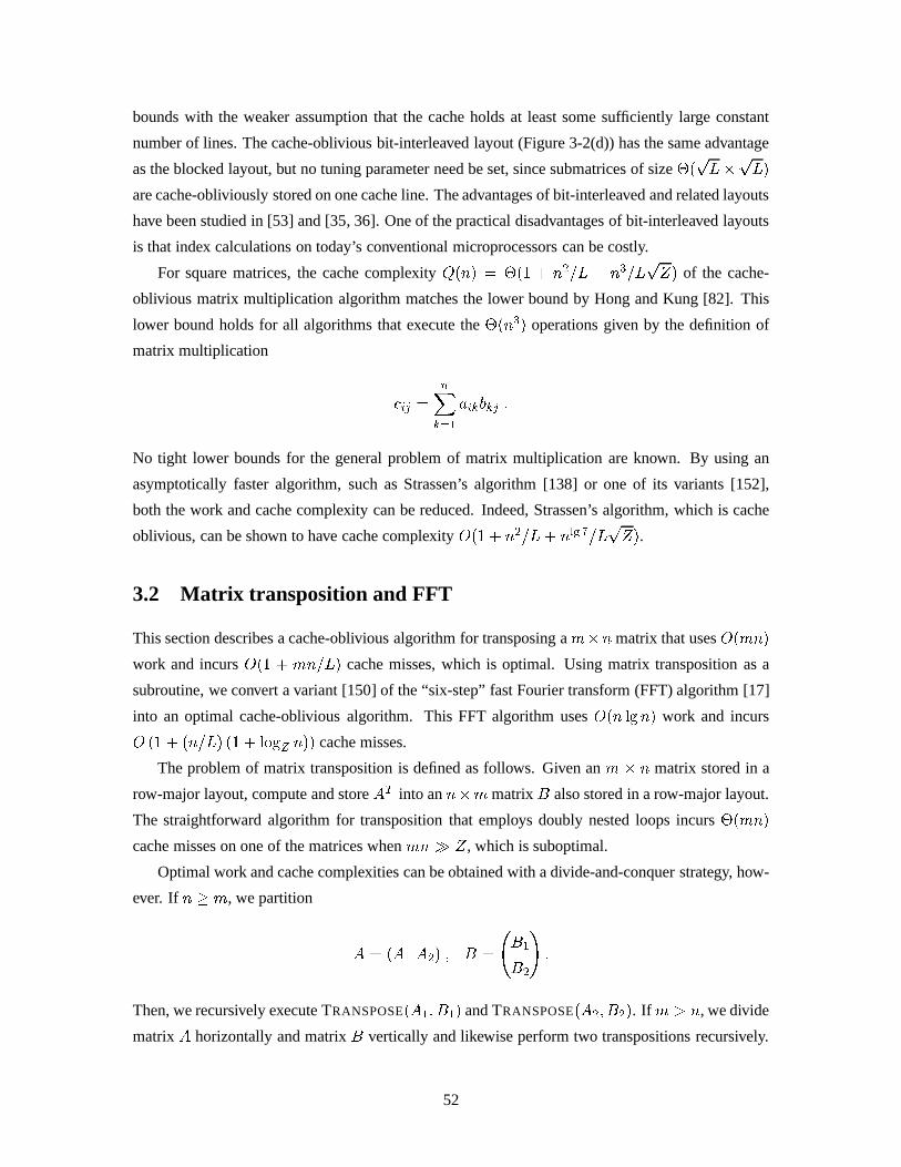
bounds with the weaker assumption that the cache holds at least some sufficiently large constant
number of lines. The cache-oblivious bit-interleaved layout (Figure 3-2(d)) has the same advantage
as the blocked layout, but no tuning parameter need be set, since submatrices of size�(pL�pL)
are cache-obliviously stored on one cache line. The advantages of bit-interleaved and related layouts
have been studied in [53] and [35, 36]. One of the practical disadvantages of bit-interleaved layouts
is that index calculations on today’s conventional microprocessors can be costly.
For square matrices, the cache complexityQ(n) = �(1 + n2=L + n3=LpZ) of the cache-
oblivious matrix multiplication algorithm matches the lower bound by Hong and Kung [82]. This
lower bound holds for all algorithms that execute the�(n3) operations given by the definition of
matrix multiplication
cij =nX
k=1
aikbkj :
No tight lower bounds for the general problem of matrix multiplication are known. By using an
asymptotically faster algorithm, such as Strassen’s algorithm [138] or one of its variants [152],
both the work and cache complexity can be reduced. Indeed, Strassen’s algorithm, which is cache
oblivious, can be shown to have cache complexityO(1 + n2=L+ nlg 7=LpZ).
3.2 Matrix transposition and FFT
This section describes a cache-oblivious algorithm for transposing am�n matrix that usesO(mn)
work and incursO(1 + mn=L) cache misses, which is optimal. Using matrix transposition as a
subroutine, we convert a variant [150] of the “six-step” fast Fourier transform (FFT) algorithm [17]
into an optimal cache-oblivious algorithm. This FFT algorithm usesO(n lgn) work and incurs
O (1 + (n=L) (1 + logZ n)) cache misses.
The problem of matrix transposition is defined as follows. Given anm � n matrix stored in a
row-major layout, compute and storeAT into ann�m matrixB also stored in a row-major layout.
The straightforward algorithm for transposition that employs doubly nested loops incurs�(mn)
cache misses on one of the matrices whenmn� Z, which is suboptimal.
Optimal work and cache complexities can be obtained with a divide-and-conquer strategy, how-
ever. Ifn � m, we partition
A = (A1 A2) ; B =
B1
B2
!:
Then, we recursively execute TRANSPOSE(A1; B1) and TRANSPOSE(A2; B2). If m > n, we divide
matrixA horizontally and matrixB vertically and likewise perform two transpositions recursively.
52

The next two lemmas provide upper and lower bounds on the performance of this algorithm.
Lemma 1 The cache-oblivious matrix-transpose algorithm usesO(mn) work and incursO(1 +
mn=L) cache misses for anm� n matrix.
Proof: We omit the proof that the algorithm usesO(mn) work. For the cache analysis, let
Q(m;n) be the cache complexity of transposing am � n matrix. We assume that the matrices
are stored in row-major order, the column-major case having a similar analysis.
Let� be a constant sufficiently small such that two submatrices of sizem�n andn�m, where
max fm;ng � �L, fit completely in the cache even if each row is stored in a different cache line.
Such a constant exists because of the tall-cache assumption. We distinguish the following three
cases.
Case I: max fm;ng � �L.
Both matrices fit inO(1) + 2mn=L lines. If � is small enough, two matrices fit completely
in cache, and we only need to read and/or write each line once in order to complete the
transposition. ThereforeQ(m;n) = O(1 +mn=L).
Case II: m � �L < n ORn � �L < m.
For this case, assume first thatm � �L < n. The transposition algorithm divides the greater
dimensionn by 2 and performs divide and conquer. At some point in the recursion,n is in
the range�L=2 � n � �L, and the whole problem fits in cache as in Case I. Because the
layout is row-major, at this point the input array hasn rows,m columns, and it is laid out
in contiguous locations, thus requiring at mostO(1 + nm=L) cache misses to be read. The
output array consists ofnm elements inm rows, where in the worst case every row lies on
a different cache line. Consequently, we incur at mostO(m + nm=L) misses for writing
the output array. Since�L � n � �L=2, the total cache complexity for this base case is
O(1 +m).
These observations yield the recurrence
Q(m;n) �(
O(1 +m) if n 2 [�L=2; �L] ;
2Q(m;n=2) +O(1) otherwise;
whose solution isQ(m;n) = O(1 +mn=L).
The casen � �L < m is analogous.
Case III: m;n > �L.
As in Case II, at some point in the recursion bothn andm are in the range[�L=2; �L]. The
whole problem fits into cache and it can be solved with at mostO(m + n + mn=L) cache
53

misses.
The cache complexity thus satisfies the recurrence
Q(m;n) �
8>><>>:
O(m+ n+mn=L) if m;n 2 [�L=2; �L] ;
2Q(m=2; n) +O(1) if m � n ;
2Q(m;n=2) +O(1) otherwise;
whose solution isQ(m;n) = O(1 +mn=L).
Theorem 2 The cache-oblivious matrix-transpose algorithm is asymptotically optimal.
Proof: For anm � n matrix, the matrix-transposition algorithm must write tomn distinct ele-
ments, which occupy at leastdmn=Le = (1 +mn=L) cache lines.
As an example of application of the cache-oblivious transposition algorithm, in the rest of this
section we describe and analyze a cache-oblivious algorithm for computing the discrete Fourier
transform of a complex array ofn elements, wheren is an exact power of2. The basic algorithm
is the well-known “six-step” variant [17, 150] of the Cooley-Tukey FFT algorithm [41]. Using
the cache-oblivious transposition algorithm, however, the FFT becomes cache-oblivious, and its
performance matches the lower bound by Hong and Kung [82].
Recall that thediscrete Fourier transform (DFT)of an arrayX of n complex numbers is the
arrayY given by
Y [i] =n�1Xj=0
X[j]!�ijn ; (3.3)
where!n = e2�p�1=n is a primitiventh root of unity, and0 � i < n.
Many known algorithms evaluate Equation (3.3) in timeO(n lgn) for all integersn [48]. In this
section, however, we assume thatn is an exact power of2, and compute Equation (3.3) according to
the Cooley-Tukey algorithm, which works recursively as follows. In the base case wheren = O(1),
we compute Equation (3.3) directly. Otherwise, for any factorizationn = n1n2 of n, we have
Y [i1 + i2n1] =
n2�1Xj2=0
240@n1�1X
j1=0
X[j1n2 + j2]!�i1j1n1
1A!�i1j2n
35!�i2j2n2 : (3.4)
Observe that both the inner and the outer summation in Equation (3.4) is a DFT. Operationally, the
computation specified by Equation (3.4) can be performed by computingn2 transforms of sizen1
54

(the inner sum), multiplying the result by the factors!�i1j2n (called thetwiddle factors[48]), and
finally computingn1 transforms of sizen2 (the outer sum).
We choosen1 to be2dlg n=2e andn2 to be2blg n=2c. The recursive step then operates as follows.
1. Pretend that input is a row-majorn1 � n2 matrix A. TransposeA in place, i.e., use the
cache-oblivious algorithm to transposeA onto an auxiliary arrayB, and copyB back ontoA.
Notice that ifn1 = 2n2, we can consider the matrix to be made up of records containing two
elements.
2. At this stage, the inner sum corresponds to a DFT of then2 rows of the transposed matrix.
Compute thesen2 DFT’s of sizen1 recursively. Observe that, because of the previous trans-
position, we are transforming a contiguous array of elements.
3. Multiply A by the twiddle factors, which can be computed on the fly with no extra cache
misses.
4. TransposeA in place, so that the inputs to the next stage is arranged in contiguous locations.
5. Computen1 DFT’s of the rows of the matrix, recursively.
6. TransposeA in place, so as to produce the correct output order.
It can be proven by induction that the work complexity of this FFT algorithm isO(n lgn). We
now analyze its cache complexity. The algorithm always operates on contiguous data, by construc-
tion. In order to simplify the analysis of the cache complexity, assume a tall cache, in which case
each transposition operation and the multiplication by the twiddle factors require at mostO(1+n=L)
cache misses. Thus, the cache complexity satisfies the recurrence
Q(n) �(
O(1 + n=L); if n � �Z ;
n1Q(n2) + n2Q(n1) +O(1 + n=L) otherwise;(3.5)
for a sufficiently small constant� chosen such that a subproblem of size�Z fits in cache. This
recurrence has solution
Q(n) = O (1 + (n=L) (1 + logZ n)) ;
which is asymptotically optimal for a Cooley-Tukey algorithm, matching the lower bound by Hong
and Kung [82] whenn is an exact power of2. As with matrix multiplication, no tight lower bounds
for cache complexity are known for the general problem of computing the DFT.
This cache-oblivious FFT algorithm will be used in FFTW in Chapter 6. Even if the ideal-
cache model is not a precise description of L1 or L2 caches, the register set of a processor is a
good approximation to an ideal cache withL = 1. Registers constitute the “cache,” the rest of
55

the memory hierarchy constitutes the “main memory,” and a compiler can usually approximate the
optimal replacement policy when allocating registers because it knows the full instruction sequence.
genfft uses this cache-oblivious FFT algorithm to produce portable C code that can be compiled
with the asymptotically optimal number of register spills, independently of the size of the register
set.
A “radix-2” or any other “constant-radix” FFT algorithm would not be asymptotically optimal.
These algorithms reduce a problem of sizen into n1 subproblems of sizen=n1, for some constant
n1, while the optimal cache-oblivious algorithm produces a nonconstant number of subproblems.
To see why a constant-radix algorithm is nonoptimal, we can solve Equation (3.5) for the case where
n1 is a constant. The resulting cache complexityO (1 + (n=L) (1 + lg(n=Z))) is asymptotically
suboptimal.
3.3 Funnelsort
Although cache oblivious, algorithms like the familiar two-way merge sort and the Cilksort variant
from Section 2.4 are not asymptotically optimal with respect to cache misses. Like the constant-
radix FFT algorithm from Section 3.2, they divide a problem into a constant number of subproblems,
and their resulting cache complexity is suboptimal. TheZ-way mergesort mentioned by Aggarwal
and Vitter [6] is optimal in terms of cache complexity, but it is cache aware. This section describes a
cache-oblivious sorting algorithm called “funnelsort.” This algorithm has an asymptotically optimal
work complexityO(n lgn), as well as an optimal cache complexityO (1 + (n=L) (1 + logZ n)) if
the cache is tall.
Like Cilksort, funnelsort is a variant of mergesort. In order to sort a (contiguous) array ofn
elements, funnelsort performs the following two steps:
1. Split the input inton1=3 contiguous arrays of sizen2=3, and sort these arrays recursively.
2. Merge then1=3 sorted sequences using an1=3-merger, which is described below.
Funnelsort differs from mergesort in the way the merge operation works. Merging is performed
by a device called ak-merger, which inputsk sorted sequences and merges them. Ak-merger
operates by recursively merging sorted sequences that become progressively longer as the algorithm
proceeds. Unlike mergesort, however, ak-merger stops working on a merging subproblem when
the merged output sequence becomes “long enough,” and it resumes working on another merging
subproblem.
Since this complicated flow of control makes ak-merger a bit tricky to describe, we explain
the operation of thek-merger pictorially. Figure 3-3 shows a representation of ak-merger, which
hask sorted sequences as inputs. Throughout its execution, thek-merger maintains the following
invariant.
56

buffer
buffer
buffer
l1
lpk
r
Figure 3-3: Illustration of ak-merger. Ak-merger (dark in the figure) is built recursively out ofpk “left”p
k-mergersl1; l2; : : : ; lpk, a series of buffers, and one “right”pk-mergerr.
Invariant The invocation of ak-merger outputs the firstk3 elements of the sorted sequence ob-
tained by merging thek input sequences.
A k-merger is built recursively out ofpk-mergers in the following way. Thek inputs are
partitioned intopk sets of
pk elements, and these sets form the input to the
pkpk-mergers
l1; l2; : : : ; lpk in the left part of the figure. The outputs of these mergers are connected to the inputs
ofpk buffers. Each buffer is a FIFO queue that can hold2k3=2 elements. Finally, the outputs of
the buffers are connected to thepk inputs of the
pk-mergerr in the right part of the figure. The
output of this finalpk-merger becomes the output of the wholek-merger. The reader should notice
that the intermediate buffers are overdimensioned. In fact, each buffer can hold2k3=2 elements,
which is twice the numberk3=2 of elements output by apk-merger. This additional buffer space
is necessary for the correct behavior of the algorithm, as will be explained below. The base case of
the recursion is ak-merger withk = 2, which producesk3 = 8 elements whenever invoked.
A k-merger operates recursively. In order to outputk3 elements, thek-merger invokesr k3=2
times. Before each invocation, however, thek-merger fills all buffers that are less than half full, i.e.,
all buffers that contain less thank3=2 elements. In order to fill bufferi, the algorithm invokes the
corresponding left mergerli once. Sinceli outputsk3=2 elements, the buffer contains at leastk3=2
elements afterli finishes.
It can be proven by induction that the work complexity of funnelsort isO(n lgn), which is
optimal for comparison-based sorting algorithms [42]. In the rest of this section, we analyze the
cache complexity of funnelsort. The goal of the analysis is to show that funnelsort onn elements
requires at mostQ(n) cache misses, where
Q(n) = O (1 + (n=L) (1 + logZ n)) ;
57

provided thatZ = (L2).
In order to prove this result, we need three auxiliary lemmas. The first lemma bounds the space
required by ak-merger.
Lemma 3 A k-merger can be laid out inO(k2) contiguous memory locations.
Proof: A k-merger requiresO(k2) memory locations for the buffers, plus the space required by
the(pk + 1) inferior
pk-mergers. The spaceS(k) thus satisfies the recurrence
S(k) � (pk + 1)S(
pk) +O(k2) ;
whose solution isS(k) = O(k2).
In order to achieve the bound onQ(n), it is important that the buffers in ak-merger be main-
tained as circular queues of sizek. This requirement guarantees that we can manage the queue
cache-efficiently, in the sense stated by the next lemma.
Lemma 4 Performingr insert and remove operations on a circular queue causesO(1+r=L) cache
misses if two cache lines are reserved for the buffer.
Proof: We reserve the two cache lines to the head and tail of the circular queue. If a new cache
line is read during a insert operation, the nextL�1 insert operations do not cause a cache miss. Con-
sequently,r insert operations incur at mostO(1 + r=L) cache misses. The argument for removals
is similar.
The next lemma bounds the number of cache missesQM incurred by ak-merger.
Lemma 5 If Z = (L2), then ak-merger operates with at mostQM(k) cache misses, where
QM(k) = O�k + k3=L+ (k3 logZ k)=L
�:
Proof: There are two cases: eitherk <p�Z or k >
p�Z, where� is a sufficiently small
constant, as usual.
Case I: Assume first thatk <p�Z.
By Lemma 3, the data structure associated with thek-merger requires at mostO(k2) =
O(�Z) contiguous memory locations, and therefore it fits into cache provided that� is small
enough. Thek-merger hask input queues, from which it loadsO(k3) elements. Letri be the
number of elements extracted from theith input queue. Sincek <p�Z andL = O(
pZ),
58

there are at leastZ=L = (k) cache lines available for the input buffers. We assume that the
optimal replacement policy reserves these cache lines for the input buffers, so that Lemma 4
applies. This assumption is wlog: We show that this replacement policy achieves the stated
bounds, and the optimal policy can only incur fewer cache misses. By Lemma 4, the total
number of cache misses for accessing the input queues is
kXi=1
O(1 + ri=L) = O(k + k3=L) :
Similarly by Lemma 4, the cache complexity of writing the output queue is at mostO(1 +
k3=L). Finally, the algorithm incurs at mostO(1 + k2=L) cache misses for touching its
internal data structures. The total cache complexity is thereforeQM(k) = O�k + k3=L
�,
completing the proof of the first case.
Case II: Assume now thatk >p�Z. In this second case, we prove by induction onk that when-
everk >p�Z, we have
QM(k) � (ck3 logZ k)=L�A(k) ; (3.6)
for some constantc > 0, whereA(k) = k(1 + 2c logZ k=L) = o(k3). This particular value
of A(k) will be justified later in the analysis.
The base case of the induction consists of values ofk such that(�Z)1=4 < k � p�Z. (It is
not sufficient to just considerk = �(pZ), sincek can become as small as�(Z1=4) in the
recursive calls.) The analysis of the first case applies, yieldingQM(k) = O�k + k3=L
�. Be-
causek2 � p�Z = (L) andk = (1), the last term dominates, andQM(k) = O�k3=L
�holds. Consequently, a large enough value ofc can be found that satisfies Inequality (3.6).
For the inductive case, letk >p�Z. Thek-merger invokes the
pk-mergers recursively.
Since (�Z)1=4 � pk � k, the inductive hypothesis can be used to bound the number
QM(pk) of cache misses incurred by the submergers. The “right” mergerr is invoked exactly
k3=2 times. The total numberl of invocations of “left” mergers is bounded byl < k3=2+2pk.
To see why, consider that every invocation of a left merger putsk3=2 elements into some
buffer. Sincek3 elements are output and the buffer space is2k2, the boundl < k3=2 + 2pk
follows.
Before invokingr, the algorithm must check every buffer to see whether it is empty. One such
check requires at mostpk cache misses, since there are
pk buffers. This check is repeated
exactlyk3=2 times, leading to at mostk2 cache misses for all checks.
59
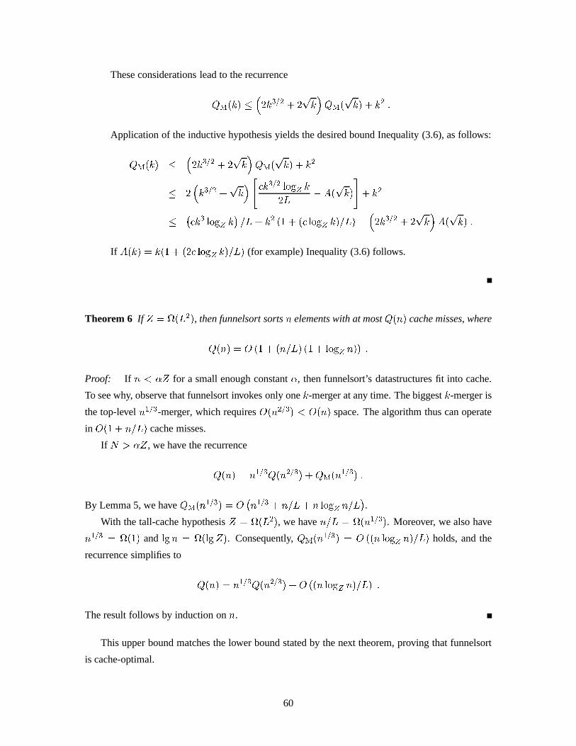
These considerations lead to the recurrence
QM(k) ��2k3=2 + 2
pk�QM(pk) + k2 :
Application of the inductive hypothesis yields the desired bound Inequality (3.6), as follows:
QM(k) ��2k3=2 + 2
pk�QM(pk) + k2
� 2�k3=2 +
pk�"ck3=2 logZ k
2L�A(
pk)
#+ k2
� �ck3 logZ k
�=L+ k2 (1 + (c logZ k)=L)�
�2k3=2 + 2
pk�A(pk) :
If A(k) = k(1 + (2c logZ k)=L) (for example) Inequality (3.6) follows.
Theorem 6 If Z = (L2), then funnelsort sortsn elements with at mostQ(n) cache misses, where
Q(n) = O (1 + (n=L) (1 + logZ n)) :
Proof: If n < �Z for a small enough constant�, then funnelsort’s datastructures fit into cache.
To see why, observe that funnelsort invokes only onek-merger at any time. The biggestk-merger is
the top-leveln1=3-merger, which requiresO(n2=3) < O(n) space. The algorithm thus can operate
in O(1 + n=L) cache misses.
If N > �Z, we have the recurrence
Q(n) = n1=3Q(n2=3) +QM(n1=3) :
By Lemma 5, we haveQM(n1=3) = O
�n1=3 + n=L+ n logZ n=L
�.
With the tall-cache hypothesisZ = (L2), we haven=L = (n1=3). Moreover, we also have
n1=3 = (1) and lgn = (lgZ). Consequently,QM(n1=3) = O ((n logZ n)=L) holds, and the
recurrence simplifies to
Q(n) = n1=3Q(n2=3) +O ((n logZ n)=L) :
The result follows by induction onn.
This upper bound matches the lower bound stated by the next theorem, proving that funnelsort
is cache-optimal.
60
Theorem 7 The cache complexity of any sorting algorithm is
Q(n) = (1 + (n=L) (1 + logZ n)) :
Proof: Aggarwal and Vitter [6] show that there is an�(n=L) logZ=L(n=Z)
�bound on the
number of cache misses made by any sorting algorithm on their “out-of-core” memory model, a
bound that extends to the ideal-cache model. The theorem can be proved by applying the tall-cache
assumptionZ = (L2) and the trivial lower bounds ofQ(n) = (1) andQ(n) = (n=L).
3.4 Distribution sort
In this section, we describe another cache-oblivious optimal sorting algorithm based on distribu-
tion sort. Like the funnelsort algorithm from Section 3.3, the distribution-sorting algorithm uses
O(n lgn) work to sortn elements, and it incursO (1 + (n=L) (1 + logZ n)) cache misses if the
cache is tall. Unlike previous cache-efficient distribution-sorting algorithms [4, 6, 120, 148, 150],
which use sampling or other techniques to find the partitioning elements before the distribution
step, our algorithm uses a “bucket splitting” technique to select pivots incrementally during the
distribution.
Given an arrayA (stored in contiguous locations) of lengthn, the cache-oblivious distribution
sort performs sortsA as follows:
1. PartitionA intopn contiguous subarrays of size
pn. Recursively sort each subarray.
2. Distribute the sorted subarrays intoq bucketsB1; : : : ; Bq of sizen1; : : : ; nq, respectively,
such that
(a) max fx j x 2 Big � minfx j x 2 Bi+1g for all 1 � i < q;
(b) ni � 2pn for all 1 � i � q.
(See below for details.)
3. Recursively sort each bucket.
4. Copy the sorted buckets to arrayA.
A stack-based memory allocator is used to exploit spatial locality.
Distribution step The goal of Step 2 is to distribute the sorted subarrays ofA into q buckets
B1; B2; : : : ; Bq. The algorithm maintains two invariants. First, each bucket holds at most2pn
elements at any time, and any element in bucketBi is smaller than any element in bucketBi+1.
61

Second, every bucket has an associated pivot. Initially, only one empty bucket exists whose pivot
is1.
The idea is to copy all elements from the subarrays into the buckets while maintaining the
invariants. We keep state information for each subarray and bucket. The state of a subarray consists
of the indexnext of the next element to be read from the subarray and the bucket numberbnum
where this element should be copied. By convention,bnum =1 if all elements in a subarray have
been copied. The state of a bucket consists of the pivot and the number of elements currently in the
bucket.
We would like to copy the element at positionnextof a subarray to bucketbnum. If this element
is greater than the pivot of bucketbnum, we would incrementbnumuntil we find a bucket for which
the element is smaller than the pivot. Unfortunately, this basic strategy has poor caching behavior,
which calls for a more complicated procedure.
The distribution step is accomplished by the recursive procedure DISTRIBUTE(i; j;m) which
distributes elements from theith through(i + m � 1)th subarrays into buckets starting fromBj.
Given the precondition that each subarrayi; i+ 1; : : : ; i+m� 1 has itsbnum � j, the execution
of DISTRIBUTE(i; j;m) enforces the postcondition that subarraysi; i+1; : : : ; i+m� 1 have their
bnum � j +m. Step 2 of the distribution sort invokes DISTRIBUTE(1; 1;pn). The following is a
recursive implementation of DISTRIBUTE:
DISTRIBUTE(i; j;m)
1 if m = 1
2 then COPYELEMS(i; j)
3 else DISTRIBUTE(i; j;m=2)
4 DISTRIBUTE(i+m=2; j;m=2)
5 DISTRIBUTE(i; j +m=2;m=2)
6 DISTRIBUTE(i+m=2; j +m=2;m=2)
In the base case, the procedure COPYELEMS(i; j) copies all elements from subarrayi that
belong to bucketj. If bucketj has more than2pn elements after the insertion, it can be split into
two buckets of size at leastpn. For the splitting operation, we use the deterministic median-finding
algorithm [42, p. 189] followed by a partition. The median-finding algorithm usesO(m) work and
incursO(1 +m=L) cache misses to find the median of an array of sizem. (In our case, we have
m = 2pn + 1.) In addition, when a bucket splits, all subarrays whosebnumis greater than the
bnumof the split bucket must have theirbnum’s incremented. The analysis of DISTRIBUTE is given
by the next two lemmas.
Lemma 8 The median ofn elements can be found cache-obliviously usingO(n) work and incur-
ring O(1 + n=L) cache misses.
62

Proof: See [42, p. 189] for the linear-time median finding algorithm and the work analysis. The
cache complexity is given by the same recurrence as the work complexity with a different base case.
Q(m) =
8>><>>:
O(1 +m=L) if m � �Z ;
Q(dm=5e) +Q(7m=10 + 6)
+O(1 +m=L) otherwise;
where� is a sufficiently small constant. The result follows.
Lemma 9 The distribute step usesO(n) work, incursO(1 + n=L) cache misses, and usesO(n)
stack space to distributen elements.
Proof: In order to simplify the analysis of the work used by DISTRIBUTE, assume that COPY-
ELEMS usesO(1) work for procedural overhead. We account for the work due to copying elements
and splitting of buckets separately. The work of DISTRIBUTE is described by the recurrence
T (c) = 4T (c=2) +O(1) :
It follows thatT (c) = O(c2), wherec =pn initially. The work due to copying elements is also
O(n).
The total number of bucket splits is at mostpn. To see why, observe that there are at most
pn
buckets at the end of the distribution step, since each bucket contains at leastpn elements. Each
split operation involvesO(pn) work and so the net contribution to the work isO(n). Thus, the
total work used by DISTRIBUTE isW (n) = O(T (pn)) +O(n) +O(n) = O(n).
For the cache analysis, we distinguish two cases. Let� be a sufficiently small constant such that
the stack space used fits into cache.
Case I: n � �Z.
The input and the auxiliary space of sizeO(n) fit into cache usingO(1 + n=L) cache lines.
Consequently, the cache complexity isO(1 + n=L).
Case II: n > �Z.
Let R(c;m) denote the cache misses incurred by an invocation of DISTRIBUTE(a; b; c) that
copiesm elements from subarrays to buckets. We again account for the splitting of buckets
separately. We first prove thatR satisfies the following recurrence:
R(c;m) �(
O(L+m=L) if c � �L ;P1�i�4R(c=2;mi) otherwise;
(3.7)
63

whereP
1�i�4mi = m.
First, consider the base casec � �L. An invocation of DISTRIBUTE(a; b; c) operates withc
subarrays andc buckets. Since there are(L) cache lines, the cache can hold all the auxiliary
storage involved and the currently accessed element in each subarray and bucket. In this
case there areO(L + m=L) cache misses. The initial access to each subarray and bucket
causesO(c) = O(L) cache misses. The cache complexity of copying them elements from
contiguous to contiguous locations isO(1+m=L). This completes the proof of the base case.
The recursive case, whenc > �L, follows immediately from the algorithm. The solution for
Equation (3.7) isR(c;m) = O(L+ c2=L+m=L).
We still need to account for the cache misses caused by the splitting of buckets. Each split
causesO(1 +pn=L) cache misses due to median finding (Lemma 8) and partitioning of
pn
contiguous elements. An additionalO(1+pn=L) misses are incurred by restoring the cache.
As proven in the work analysis, there are at mostpn split operations.
By addingR(pn; n) to the split complexity, we conclude that the total cache complexity of
the distribution step isO(L+ n=L+pn(1 +
pn=L)) = O(n=L).
Theorem 10 Distribution sort usesO(n lgn) work and incursO(1 + (n=L) (1 + logZ n)) cache
misses to sortn elements.
Proof: The work done by the algorithm is given by
W (n) =pnW (
pn) +
qXi=1
W (ni) +O(n) ;
where eachni � 2pn and
Pni = n. The solution to this recurrence isW (n) = O(n lgn).
The space complexity of the algorithm is given by
S(n) � S(2pn) +O(n) ;
where theO(n) term comes from Step 2. The solution to this recurrence isS(n) = O(n).
The cache complexity of distribution sort is described by the recurrence
Q(n) �
8>><>>:
O(1 + n=L) if n � �Z ;pnQ(pn) +
Pqi=1Q(ni) otherwise;
+O(1 + n=L)
64

where� is a sufficiently small constant such that the stack space used by a sorting problem of size
�Z, including the input array, fits completely in cache. The base casen � �Z arises when both
the input arrayA and the contiguous stack space of sizeS(n) = O(n) fit in O(1 + n=L) cache
lines of the cache. In this case, the algorithm incursO(1 + n=L) cache misses to touch all involved
memory locations once. In the case wheren > �Z, the recursive calls in Steps 1 and 3 cause
Q(pn) +
Pqi=1Q(ni) cache misses andO(1 + n=L) is the cache complexity of Steps 2 and 4, as
shown by Lemma 9. The theorem now follows by solving the recurrence.
3.5 Other cache models
In this section we show that cache-oblivious algorithms designed in the two-level ideal-cache model
can be efficiently ported to other cache models. We show that algorithms whose complexity bounds
satisfy a simple regularity condition (including all algorithms heretofore presented) can be ported
to less-ideal caches incorporating least-recently-used (LRU) or first-in, first-out (FIFO) replace-
ment policies [79, p. 378]. We argue that optimal cache-oblivious algorithms are also optimal for
multilevel caches. Finally, we present simulation results proving that optimal cache-oblivious algo-
rithms satisfying the regularity condition are also optimal (in expectation) in the previously studied
SUMH [11, 148] and HMM [4] models. Thus, all the algorithmic results in this chapter apply to
these models, matching the best bounds previously achieved.
3.5.1 Two-level models
Many researchers, such as [6, 82, 149], employ two-level models similar to the ideal-cache model,
but without an automatic replacement strategy. In these models, data must be moved explicitly
between the the primary and secondary levels “by hand.” We define a cache complexity bound
Q(n;Z;L) to beregular if
Q(n;Z;L) = O(Q(n; 2Z;L)) : (3.8)
We now show that optimal algorithms in the ideal-cache model whose cache complexity bounds are
regular can be ported to these models to run using optimal work and incurring an optimal expected
number of cache misses.
The first lemma shows that the optimal and omniscient replacement strategy used by an ideal
cache can be simulated efficiently by the LRU and FIFO replacement strategies.
Lemma 11 Consider an algorithm that causesQ�(n;Z;L) cache misses on a problem of sizen
using a(Z;L) ideal cache. Then, the same algorithm incursQ(n;Z;L) � 2Q�(n;Z=2; L) cache
misses on a(Z;L) cache that uses either LRU or FIFO replacement.
65

Proof: Sleator and Tarjan [133] have shown that the cache misses on a(Z;L) cache using LRU
replacement is(Z=(Z � Z� + 1))-competitive with optimal replacement on a(Z�; L) ideal if both
caches start with an empty cache. It follows that the number of misses on a(Z;L) LRU-cache is
at most twice the number of misses on a(Z=2; L) ideal-cache. The same argument holds for FIFO
caches.
Corollary 12 For algorithms with regular cache complexity bounds, the asymptotic number of
cache misses is the same for LRU, FIFO, and optimal replacement.
Proof: Follows directly from Lemma 11 and the regularity condition Equation (3.8).
Since previous two-level models do not support automatic replacement, to port a cache-oblivious
algorithms to them, we implement a LRU (or FIFO) replacement strategy in software.
Lemma 13 A (Z;L) LRU-cache (or FIFO-cache) can be maintained usingO(Z) primary memory
locations such that every access to a cache line in primary memory takesO(1) expected time.
Proof: Given the address of the memory location to be accessed, we use a2-universal hash func-
tion [114, p. 216] to maintain a hash table of cache lines present in the primary memory. TheZ=L
entries in the hash table point to linked lists in a heap of memory containingZ=L records corre-
sponding to the cache lines. The2-universal hash function guarantees that the expected size of a
chain isO(1). All records in the heap are organized as a doubly linked list in the LRU order (or
singly linked for FIFO). Thus, the LRU (FIFO) replacement policy can be implemented inO(1)
expected time usingO(Z=L) records ofO(L) words each.
Theorem 14 An optimal cache-oblivious algorithm with a regular cache-complexity bound can be
implemented optimally in expectation in two-level models with explicit memory management.
Proof: Follows from Corollary 12 and Lemma 13.
Consequently, our cache-oblivious algorithms for matrix multiplication, matrix transpose, FFT,
and sorting are optimal in two-level models.
3.5.2 Multilevel ideal caches
We now show that optimal cache-oblivious algorithms also perform optimally in computers with
multiple levels of ideal caches. Moreover, Theorem 14 extends to multilevel models with explicit
memory management.
The h(Z1; L1); (Z2; L2); : : : ; (Zr; Lr)i ideal-cache modelconsists of an arbitrarily large
main memory and a hierarchy ofr caches, each of which is managed by an optimal replacement
66

strategy. The model assumes that the caches satisfy theinclusion property [79, p. 723], which
says that fori = 1; 2; : : : ; r � 1, the values stored in cachei are also stored in cachei + 1. The
performance of an algorithm running on an input of sizen is measured by its work complexity
W (n) and its cache complexitiesQi(n;Zi; Li) for each leveli = 1; 2; : : : ; r.
Theorem 15 An optimal cache-oblivious algorithm in the ideal-cache model incurs an asymptoti-
cally optimal number of cache misses on each level of a multilevel cache with optimal replacement.
Proof: The theorem follows directly from the definition of cache obliviousness and the optimality
of the algorithm in the two-level ideal-cache model.
Theorem 16 An optimal cache-oblivious algorithm with a regular cache-complexity bound incurs
an asymptotically optimal number of cache misses on each level of a multilevel cache with LRU,
FIFO, or optimal replacement.
Proof: Follows from Corollary 12 and Theorem 16.
3.5.3 The SUMH model
In 1990 Alpern et al. [11] presented the uniform memory hierarchy model (UMH), a parameterized
model for a memory hierarchy. In the UMH�;�;b(l) model, for integer constants�; � > 1, the size
of the ith memory level isZi = ��2i and the line length isLi = �i. A transfer of one�l-length
line between the caches on levell andl + 1 takes�l=b(l) time. The bandwidth functionb(l) must
be nonincreasing and the processor accesses the cache on level1 in constant time per access. An
algorithm given for the UMH model must include a schedule that, given for a particular set of input
variables, tells exactly when each block is moved along which of the buses between caches. Work
and cache misses are folded into one cost measureT (n). Alpern et al. prove that an algorithm
that performs the optimal number of I/O’s at all levels of the hierarchy does not necessarily run in
optimal time in the UMH model, since scheduling bottlenecks can occur when all buses are active.
In the more restrictive SUMH model [148], however, only one bus is active at a time. Consequently,
we can prove that optimal cache-oblivious algorithms run in optimal expected time in the SUMH
model.
Lemma 17 A cache-oblivious algorithm withW (n)work andQ(n;Z;L) cache misses on a(Z;L)-
ideal cache can be executed in the SUMH�;�;b(l) model in expected time
T (n) = O�W (n) +
r�1Xi=1
�i
b(i)Q(n; �(Zi); Li)
�;
67

whereZi = ��2i, Li = �i, andZr is big enough to hold all elements used during the execution of
the algorithm.
Proof: Use the memory at theith level as a cache of sizeZi = ��2i with line lengthLi = �i and
manage it with software LRU described in Lemma 13. Therth level is the main memory, which is
direct mapped and not organized by the software LRU mechanism. An LRU-cache of size�(Zi)
can be simulated by theith level, since it has sizeZi. Thus, the number of cache misses at level
i is 2Q(n; �(Zi); Li), and each takes�i=b(i) time. Since only one memory movement happens at
any point in time, and there areO(W (n)) accesses to level1, the lemma follows by summing the
individual costs.
Lemma 18 Consider a cache-oblivious algorithm whose work on a problem of sizen is lower-
bounded byW �(n) and whose cache complexity is lower-bounded byQ�(n;Z;L) on an (Z;L)
ideal-cache. Then, no matter how data movement is implemented in SUMH�;�;b(l), the time taken
on a problem of sizen is at least
T (n) = �W �(n) +
rXi=1
�i
b(i)Q�(n;�(Zj); Li)
�;
whereZi = ��2i, Li = �i andZr is big enough to hold all elements used during the execution of
the algorithm.
Proof: The optimal scheduling of the data movements does not need to obey the inclusion prop-
erty, and thus the number ofith-level cache misses is at least as large as for an ideal cache of sizePij=1 Zi = O(Zi). SinceQ�(n;Z;L) lower-bounds the cache misses on a cache of sizeZ, at least
Q�(n;�(Zi); Li) data movements occur at leveli, each of which takes�i=b(i) time. Since only one
movement can occur at a time, the total cost is the maximum of the work and the sum of the costs
at all the levels, which is within a factor of2 of their sum.
Theorem 19 A cache-oblivious algorithm that is optimal in the ideal-cache model and whose
cache-complexity is regular can be executed optimal expected time in the SUMH�;�;b(l) model.
Proof: The theorem follows directly from regularity and Lemmas 17 and 18.
3.6 Related work
In this section, we discuss the origin of the notion of cache-obliviousness. We also give an overview
of other hierarchical memory models.
68

Our research group at MIT noticed as far back as 1994 that divide-and-conquer matrix mul-
tiplication was a cache-optimal algorithm that required no tuning, but we did not adopt the term
“cache-oblivious” until 1997. This matrix-multiplication algorithm, as well as a cache-oblivious
algorithm for LU-decomposition without pivoting, eventually appeared in [26]. Shortly after leav-
ing our research group, Toledo [143] independently proposed a cache-oblivious algorithm for LU-
decomposition, but with pivoting. Forn � n matrices, Toledo’s algorithm uses�(n3) work and
incurs�(1 + n2=L + n3=LpZ) cache misses. My own FFTW Fourier transform library em-
ploys a register-allocation and scheduling algorithm inspired by the cache-oblivious FFT algorithm.
The general idea that divide-and-conquer enhances memory locality has been known for a long
time [132].
Previous theoretical work on understanding hierarchical memories and the I/O-complexity of al-
gorithms has been studied in cache-aware models lacking an automatic replacement strategy. Hong
and Kung [82] use the red-blue pebble game to prove lower bounds on the I/O-complexity of ma-
trix multiplication, FFT, and other problems. The red-blue pebble game models temporal locality
using two levels of memory. The model was extended by Savage [129] for deeper memory hierar-
chies. Aggarwal and Vitter [6] introduced spatial locality and investigated a two-level memory in
which a block ofP contiguous items can be transferred in one step. They obtained tight bounds for
matrix multiplication, FFT, sorting, and other problems. The hierarchical memory model (HMM)
by Aggarwal et al. [4] treats memory as a linear array, where the cost of an access to element at
locationx is given by a cost functionf(x). The BT model [5] extends HMM to support block
transfers. The UMH model by Alpern et al. [11] is a multilevel model that allows I/O at different
levels to proceed in parallel. Vitter and Shriver introduce parallelism, and they give algorithms for
matrix multiplication, FFT, sorting, and other problems in both a two-level model [149] and sev-
eral parallel hierarchical memory models [150]. Vitter [147] provides a comprehensive survey of
external-memory algorithms.
3.7 Conclusion
In this chapter, we discussed the notion of cache-obliviousness, and we presented optimal cache-
oblivious algorithms for rectangular matrix transpose and multiplication, FFT, and sorting. Cache-
oblivious algorithms are inherently portable, because they depend on no tuning parameters, and
optimal cache-oblivious algorithms enable portability of performance across systems with diverse
memory hierarchies. We learned that divide and conquer can yield algorithms that are good from
both Cilk’s perspective, because they have short critical path, and from the point of view of the
memory hierarchy, because they achieve the optimal cache complexity.
Far from answering all questions in portable high performance, however, this chapter open more
problems than I am capable of solving. Intuitively, I would expect the cache complexity of cache-
69

aware algorithms to be inherently lower than the complexity of cache-oblivious algorithms, but the
results of this chapter contradict this intuition. Do optimal cache-oblivious algorithms exist for all
problems, or can we find a problem for which cache-aware algorithms are inherently better? This
problem is open for future research.
A second set of questions arises when we try to run a cache-oblivious algorithm in parallel, for
example using Cilk. Running these algorithms in parallel would produce a formidable combination
of portability and high performance, because the resulting program would be high-performance and
yet insensitive to both the number of processors and the memory hierarchy. Unfortunately, things
are not so easy. The analysis Cilk scheduler offers no performance guarantees if Cilk threads are
delayed by cache misses, and conversely, the analysis of cache-oblivious algorithm offer no cache-
complexity guarantees in a Cilk environment where the scheduler moves threads across the parallel
machine. The problem of combining Cilk with cache-oblivious algorithms is not completely open,
however, and we shall discuss a possible solution in Chapter 4.
The ideal-cache model is not an adequate model of write-through caches. In many modern pro-
cessor, the L1 cache iswrite-through, i.e., it transmits written values to the L2 cache immediately.
With write-through caches, we can no longer argue that once a problem fits into cache no further
misses are incurred, since the cache incurs a “miss” at every write operation. We currently do not
know how to account for write-through caches in our theory of cache-oblivious algorithms.
70
Chapter 4
Portable parallel memory
In this chapter we attempt to marry Cilk with cache-oblivious algorithms. In Cilk, we can write
high-performance programs that run efficiently with varying degrees of parallelism. The theory of
cache-oblivious algorithms allows us to design fast algorithms that are insensitive to the parameters
of the memory hierarchy. What happens when we code the cache-oblivious algorithms in Cilk and
run them on a parallel machine? Specifically, consider the following two questions.
1. Can we preserve Cilk’s performance guarantees and its empirical efficiency if we augment the
Cilk scheduler with a cache? The Cilk theory of Section 2.3 does not mention caches at all.
The execution-time upper bound from [25] does not hold in the presence of caches, because
the proof does not account for the time spent in servicing cache misses.
2. Is the cache complexity preserved when a program is executed in parallel? For example, if
work is moved from one processor to another, the contents of the first cache are unavailable
to the destination processor, and communication between caches is necessary for the correct
execution of the program.
The answer to these two questions seems to depend crucially on the memory model that we use.
A memory modelis a specification of how memory behaves in a computer system. To see why a
good memory model is important, imagine executing a Cilk program on a network of workstations
in which each processor operates within its own memory and no attempt is ever made to synchronize
the memory contents. Such a system would be very fast, since workstations do not communicate at
all, but most likely useless since processors cannot see each other’s results. On the other extreme,
thesequential consistencymodel [96] dictates that the whole memory of the machine behave as a
single black box, so that every processor sees the same order of memory events (reads and writes).
Sequential consistency appears at first sight to be the ideal memory model, because it preserves
This chapter represents joint work with Bobby Blumofe, Chris Joerg, and Charles Leiserson, and Keith Randall. Apreliminary version appears in [27, 26].
71

the black-box abstraction of a single memory, but unfortunately, sequential consistency has a price.
It is generally believed [79] that sequential consistency imposes major inefficiencies in an imple-
mentation. (See [81] for the opposite view, however.) Consequently, many researchers have tried
to relax the requirements of sequential consistency in exchange for better performance and ease of
implementation. For example,processor consistency[70] is a model where every processor can
have an independent view of memory, andrelease consistency[64] is a model where the memory
becomes consistent only when certain synchronizing operations are performed. See [1] for a good
tutorial on this subject.
In this chapter, we focus on a memory model calledlocation consistency.1 Location consistency
is relevant to portable high performance because it is the memory model maintained by theBACKER
coherence algorithm, and a combination of BACKER and Cilk executes a cache-oblivious Cilk pro-
gram maintaining both the performance guarantees of Cilk and the program’s cache complexity.
Specifically, we prove that a Cilk program with workT1, critical pathT1, and cache-complexity
Q(Z;L) runs onP processors in expected time
TP = O((T1 + �Q(Z;L))=P + �ZT1=L) ;
where� is the cost of transferring one cache line between main memory and the cache. To my
knowledge, the combination of Cilk andBACKER is the only shared-memory programming system
algorithm with any sort of performance guarantee. While the BACKER coherence algorithm is
simplistic and does not attempt optimizations, it has been implemented in the Cilk-3 runtime system
with encouraging empirical results [27].
To illustrate the concepts behind location consistency, consider again thematrixmul program
from Section 2.4. Like any Cilk multithreaded computation [28], the parallel instruction stream of
matrixmul can be viewed as a “spawn tree” of procedures broken into a directed acyclic graph, or
dag, of “threads.” Thespawn treeis exactly analogous to a traditional call tree. When a procedure,
such asmatrixmul performs a spawn, the spawned procedure becomes a child of the procedure that
performed the spawn. Each procedure is broken bysync statements into nonblocking sequences of
instructions, calledthreads, and the threads of the computation are organized into a dag representing
the partial execution order defined by the program. Figure 4-1 illustrates the structure of the dag
for matrixmul. Each vertex corresponds to a thread of the computation, and the edges define the
partial execution order. The syncs in lines 21 and 23 break the procedurematrixmul into three
threadsu, v, andw, which correspond respectively to the partitioning and spawning of subproblems
M0;M1; : : : ;M7 in lines 2–20, the spawning of the additionS in line 22, and the return in line 25.
1Location consistency is often called coherence in the literature [79]. It isnot the model with the same name intro-duced by Gao and Sarkar [61]. See [54] for a justification of this terminology.
72

u v w
SM7M6M5M4M3M2M1M0
Figure 4-1: Dag generated by the execution of the matrix multiplication program in Figure 2-4. Some edgeshave been omitted for clarity.
Location-consistent shared memory is a natural consistency model to support a shared-memory
program such asmatrixmul. Certainly, sequential consistency [96] can guarantee the correctness of
the program, but a closer look at the precedence relation given by the dag reveals that a much weaker
consistency model suffices. Specifically, the 8 recursively spawned childrenM0;M1; : : : ;M7 need
not have the same view of shared memory, because the portion of shared memory that each writes
is neither read nor written by the others. On the other hand, the parallel addition oftmp into R
by the computationS requiresS to have a view in which all of the writes to shared memory by
M0;M1; : : : ;M7 have completed.
The intuition behind location consistency is that each memory location sees values that are
consistent with some serial execution order of the dag, but two different locations may see different
serial orders. Thus, the writes performed by a thread are seen by its successors, but threads that are
incomparable in the dag may or may not see each other’s writes. Inmatrixmul, the computationS
sees the writes ofM0;M1; : : : ;M7, because all the threads ofS are successors ofM0;M1; : : : ;M7,
but since theMi are incomparable, they cannot depend on seeing each others writes. We shall define
location consistency precisely in Section 4.2.
All threads of a multithreaded computation should have access to a single, shared virtual address
space, and in order to support such a shared-memory abstraction on a computer with physically
distributed memory, the runtime scheduler must be coupled with a coherence algorithm. For our
BACKER coherence algorithm, we assume that each processor’s memory is divided into two regions,
each containing lines of shared-memory objects. One region is acacheof sizeZ, partitioned into
Z=L lines of lengthL containing locations that have been recently accessed by that processor.
The rest of each processors’ memory is maintained as amain memoryof locations that have been
allocated in the virtual address space. Each allocated line is assigned to the main memory of a
processor chosen by hashing the cache line’s virtual address. In order for a processor to operate on
a location, the location must be resident in the processor’s cache; otherwise, a cache miss occurs,
and BACKER must “fetch” the correct cache line from main memory into the cache. We assume that
when a cache miss occurs, no progress can be made on the computation during the time it takes to
service the miss, and the miss time may vary due to congestion of concurrent accesses to the main
memory. Like in the ideal-cache model of Chapter 3, we shall further assume that lines in the cache
73

are maintained using the LRU (least-recently-used) [88] heuristic. In addition to servicing cache
misses, BACKER must “reconcile” cache lines between the processor caches and the main memory
so that the semantics of the execution obey the assumptions of location consistency.
The remainder of this chapter is organized as follows. Section 4.1 combines the Cilk perfor-
mance model and the ideal-cache model, and states the performance of BACKER precisely. Sec-
tion 4.2 gives a precise definition of location consistency and describes the BACKER coherence al-
gorithm. Section 4.3 analyzes the execution time of fully strict [25] multithreaded algorithms when
the execution is scheduled by the randomized work-stealing scheduler and location consistency is
maintained by the BACKER coherence algorithm. Section 4.4 analyzes the space requirements of
parallel divide-and-conquer algorithms. Finally, Section 4.5 offers some comparisons with other
consistency models.
4.1 Performance model and summary of results
This section defines performance measures for location-consistent Cilk programs, and states the
main results of this chapter formally. We define thetotal workT1(Z;L) as the serial execution time
on a machine with a(Z;L) cache, and we clarify the meaning of critical-path length in programs
that use shared memory. We state bounds on the execution time and cache misses of fully strict [25]
programs executed by Cilk in conjunction with the BACKER coherence algorithm. We state bounds
on the space requirements of parallel divide-and-conquer algorithms. As an example of application,
we apply these results to the cache-oblivious Cilk programmatrixmul.
In order to model the performance of multithreaded algorithms that use location-consistent
shared memory, it is important to observe that running times will vary as a function of the cache
sizeZ and of the line sizeL, and consequently we must introduce measures that account for this
dependence. Consider a(Z;L) cache, which containsH = Z=L lines of sizeL. We call quantity
H the cache height. Let � be the time to service a cache miss in the serial execution. For exam-
ple,� might be proportional to the line sizeL, but here we do not assume any specific relationship
between� andL.
Consider again the multithreaded computation (such as the one in Figure 4-1) that results when
a given multithreaded algorithm is used to solve a given problem. We shall define a new work
measure, the “total work,” that accounts for the cost of cache misses in the serial execution of the
computation, as follows. We associate a weight with each instruction of the dag. Each instruction
that generates a cache miss in the one-processor execution with the standard, depth-first serial ex-
ecution order has weight� + 1, and all other instructions have weight1. The total work, denoted
T1(Z;L), is the total weight of all instructions in the dag, which corresponds to the serial execution
time if cache misses take� units of time to be serviced. We shall continue to letT1 denote the num-
ber of instructions in the dag, but for clarity, we shall refer toT1 as thecomputational work. (The
74

computational workT1 corresponds to the serial execution time if all cache misses take zero time
to be serviced.) To relate these measures, we define theserial cache complexity, denotedQ(Z;L),
to be the number of cache misses taken in the serial execution (that is, the number of instructions
with weight � + 1). This measure is the same as the cache complexity of Chapter 3. Thus, we
haveT1(Z;L) = T1 + �Q(Z;L). The total work therefore translates both the work and the cache
complexity of Chapter 3 into units of execution time. This definition is useful because from the
point of view of the Cilk scheduler it does not matter whether threads spend time in computational
work or in waiting for cache misses.
The quantityT1(Z;L) is an unusual measure. UnlikeT1, it depends on the serial execution order
of the computation. The quantityT1(Z;L) further differs fromT1 in thatT1(Z;L)=P is not a lower
bound on the execution time forP processors. It is possible to construct a computation containing
P subcomputations that run onP separate processors in which each processor repeatedly accesses
H different cache lines in sequence. Consequently, with(Z;L) caches, no processor ever misses,
except to warm up the cache at the start of the computation. If we run the same computation serially
with a cache of heightH (or any size less thanHP ), however, the necessary multiplexing among
tasks can cause numerous cache misses. Consequently, for this computation, the execution time
with P processors is much less thanT1(Z;L)=P . In this dissertation, we shall forgo the possibility
of obtaining such superlinear speedup on computations. Instead, we shall simply attempt to obtain
linear speedup.
Critical-path length can likewise be split into two notions. We define thetotal critical-path
length, denotedT1(Z;L), to be the maximum over all directed paths in the computational dag, of
the time, including cache misses, to execute along the path by a single processor with an(Z;L)
cache. Thecomputational critical-path lengthT1 is the same, but where misses cost zero time.
Both T1 andT1(Z;L) are lower bounds on execution time. AlthoughT1(Z;L) is the stronger
lower bound, it appears difficult to compute and analyze, and our upper-bound results will be char-
acterized in terms ofT1, which we shall continue to refer to simply as the critical-path length.
The main result of this chapter is the analysis of the execution time of “fully strict” multi-
threaded algorithms that use location consistent shared memory. A multithreaded computation is
fully strict [25] if every dependency edge goes from a procedure to either itself or its parent pro-
cedure. All Cilk-5 computations are fully strict, because a Cilk procedure can return a value only
to its parent, but not to its other ancestors. (This constraint is enforced by the call/return semantics
of Cilk.) Consequently, the analysis applies to all Cilk programs. The multithreaded algorithm is
executed on a parallel computer withP processors, each with a(Z;L) cache, and a cache miss
that encounters no congestion is serviced in� units of time. The execution is scheduled by the
Cilk work-stealing scheduler and location consistency is maintained by the BACKER coherence al-
gorithm. In addition, we assume that accesses to shared memory are distributed uniformly and
independently over the main memory—often a plausible assumption, since BACKER hashes cache
75

lines to the main memory. The following theorem bounds the parallel execution time.
Theorem 20 Consider any fully strict multithreaded computation executed onP processors, each
with an LRU cache of heightH, using the Cilk work-stealing scheduler in conjunction with the
BACKER coherence algorithm. Let� be the service time for a cache miss that encounters no con-
gestion, and assume that accesses to the main memory are random and independent. Suppose the
computation hasT1 computational work,Q(Z;L) serial cache misses,T1(Z;L) = T1 + �Q(Z;L)
total work, andT1 critical-path length. Then for any� > 0, the execution time isO(T1(Z;L)=P +
�HT1 + �P lgP + �H lg(1=�)) with probability at least1� �. Moreover, the expected execution
time isO(T1(Z;L)=P + �HT1).
Proof: See Section 4.3.
This theorem enables us to design high-performance portable programs by designing algorithms
with optimal work, critical path, and cache complexity. In the cases where we cannot optimize all
three quantities simultaneously, Theorem 20 gives a model to investigate the tradeoffs. For example,
the critical path ofmatrixmul is �(lg2 n). We could write a matrix multiplication program with
critical path�(lgn) by spawning a separate thread to compute each element of the output array,
where each thread spawns a divide-and-conquer addition. This algorithm would have a�(n3)
cache complexity, however, whilematrixmul’s complexity is�(n3)=(LpZ). For large values
of n, Theorem 20 predicts thatmatrixmul is faster.
Theorem 20 is not as strong a result as we would like to prove, because accesses to the main
memory are not necessarily independent. For example, threads may concurrently access the same
cache lines by algorithm design. We can artificially solve this problem by insisting, as does the
EREW-PRAM model, that the algorithm performs exclusive accesses only. More seriously, how-
ever, congestion delay in accessing the main memory can cause the computation to be scheduled
differently than if there were no congestion, thereby perhaps causing more congestion to occur. It
may be possible to prove our bounds for a hashed main memory without making this independence
assumption, but we do not know how at this time. The problem with independence does not seem
to be serious in practice, and indeed, given the randomized nature of our scheduler, it is hard to
conceive of how an adversary can actually take advantage of the lack of independence implied by
hashing to slow the execution. Although our results are imperfect, we are actually analyzing the
effects of congestion, and thus our results are much stronger than if we had assumed, for example,
that accesses to the main memory independently suffer Poisson-distributed delays.
In this chapter, we also analyze the number of cache misses that occur during algorithm exe-
cution. This is the parallel analogue of the cache complexity. Again, execution is scheduled with
the Cilk work-stealing scheduler and location consistency is maintained by the BACKER coherence
algorithm, and we assume that accesses to main memory are random and independent. A bound on
76

the number of cache misses is stated by the next corollary.
Corollary 21 Consider any fully strict multithreaded computation executed onP processors, each
with an LRU cache of heightH, using the Cilk work-stealing scheduler in conjunction with the
BACKER coherence algorithm. Assume that accesses to the main memory are random and indepen-
dent. Suppose the computation hasQ(Z;L) serial cache misses andT1 critical-path length. Then
for any � > 0, the number of cache misses is at mostQ(Z;L) + O(HPT1 + HP lg(1=�)) with
probability at least1 � �. Moreover, the expected number of cache misses is at mostQ(Z;L) +
O(HPT1).
Proof: See Section 4.3.
For example, the total number of cache misses incurred bymatrixmul when multiplyingn�nmatrices usingP processors isO(1+n2=L+n3=(L
pZ)+HP lg2 n), assuming that the indepen-
dence assumption for the main memory holds.
Space utilization of Cilk programs is relevant to portable high performance, too. If a program
exhausts memory when run in parallel, it is not portable no matter how fast it is. In this chapter, we
analyze the space requirements of “simple” multithreaded algorithms that use location-consistent
shared memory. We assume that the computation is scheduled by a scheduler, such as the work-
stealing algorithm, that maintains the “busy-leaves” property [25, 30]. For a given simple multi-
threaded algorithm, letS1 denote the space required by the standard, depth-first serial execution of
the algorithm to solve a given problem. In previous work, Blumofe has shown that the space used by
aP -processor execution is at mostS1P in the worst case [25, 30]. We improve this characterization
of the space requirements, and we provide a much stronger upper bound on the space requirements
of “regular” divide-and-conquer multithreaded algorithms, in which each thread divides a problem
of sizen into a subproblems, each of sizen=b for some constantsa � 1 andb > 1, and then it
recursively spawns child threads to solve each subproblem.
Theorem 22 Consider any regular divide-and-conquer multithreaded algorithm executed onP
processors using a busy-leaves scheduler. Suppose that each thread, when spawned to solve a
problem of sizen, allocatess(n) space, and ifn is larger than some constant, then the thread di-
vides the problem intoa subproblems each of sizen=b for some constantsa � 1 andb > 1. Then,
the total amountSP (n) of space taken by the algorithm in the worst case when solving a problem
of sizen can be determined as follows:2
1. If s(n) = �(lgk n) for some constantk � 0, thenSP (n) = �(P lgk+1(n=P )).
2Other cases exist besides those given here.
77

2. If s(n) = O(nlogb a��) for some constant� > 0, thenSP (n) = �(Ps(n=P 1= logb a)), if,
in addition, s(n) satisfies the regularity condition 1s(n=b) � s(n) � a 2s(n=b) for some
constants 1 > 1 and 2 < 1.
3. If s(n) = �(nlogb a), thenSP (n) = �(s(n) lgP ).
4. If s(n) = (nlogb a+�) for some constant� > 0, thenSP (n) = �(s(n)), if, in addition,s(n)
satisfies the regularity condition thats(n) � a s(n=b) for some constant > 1.
Proof: See Section 4.4.
For example, Theorem 22 applies tomatrixmul with a = 8, b = 2, ands(n) = O(n2). From
Case 2, we see that multiplyingn�n matrices onP processors uses only�(n2P 1=3) space, which
is tighter than theO(n2P ) result obtained by directly applying theS1P bound.
4.2 Location consistency and the BACKER coherence algorithm
In this section we give a precise definition of location consistency, and we describe the BACKER
[27] coherence algorithm for maintaining this memory model. Location consistency is a relaxed
consistency model for distributed shared memory, and the BACKER algorithm can maintain location
consistency for multithreaded computations that execute on a parallel computer with physically
distributed memory. In this chapter we give a simplified definition of location consistency. Chapter 5
offers an equivalent definition (Definition 48) in the more formalcomputation-centrictheory of
memory models.
Shared memory consists of a set oflocations that instructions can read and write. When an
instruction performs a read of a location, it receives some value, but the particular value it receives
depends upon the consistency model. As its name suggests, location consistency is defined sepa-
rately for each location in shared memory.
Definition 23 Let C be the dag of a multithreaded computation. The shared memoryM of the
computationC is location consistentif for all locationsl there exists a topological sortTl ofC such
that every read operation on locationl returns the value of the last write to locationl occurring in
Tl.
In previous work [27, 26], we presenteddag consistency, a memory model strictly weaker than
location consistency. Afterwards, I showed anomalies in the definition of dag consistency, and
I argued that location consistency is the weakest reasonable memory model [54]. In Chapter 5,
we will use the “computation-centric” theoretical framework to understand the differences among
location consistency, dag consistency, and other memory models.
78
We now describe the BACKER coherence algorithm from [27], in which versions of shared-
memory locations can reside simultaneously in any of the processor caches and the main memory.
Each processor’s cache contains locations recently used by the threads that have executed on that
processor, and the main memory provides default global storage for each location. In order for a
thread executing on the processor to read or write a location, the location must be in the processor’s
cache. Each location in the cache has adirty bit to record whether the location has been modified
since it was brought into the cache.
BACKER uses three basic operations to manipulate shared-memory locations: fetch, reconcile,
and flush. Afetch copies an location from the main memory to a processor cache and marks the
cached location as clean. Areconcilecopies a dirty location from a processor cache to the main
memory and marks the cached location as clean. Finally, aflush removes a clean location from a
processor cache.
The BACKER coherence algorithm operates as follows. When the user code performs a read or
write operation on a location, the operation is performed directly on a cached copy of the location.
If the location is not in the cache, it is fetched from the main memory before the operation is
performed. If the operation is a write, the dirty bit of the location is set. To make space in the cache
for a new location, a clean location can be removed by flushing it from the cache. To remove a dirty
location, BACKER first reconciles and then flushes it.
Besides performing these basic operations in response to user reads and writes, BACKER per-
forms additional reconciles and flushes to enforce location consistency. For each edgeu! v in the
computation dag, if nodesu andv are executed on different processors, sayp andq, then BACKER
causesp to reconcile all its cached locations after executingu but before enablingv, and it causesq
to reconcile and flush its entire cache before executingv. Note that ifq’s cache is flushed for some
other reason afterp has reconciled its cache but beforeq executesv (perhaps because of another
interprocessor dag edge), it need not be flushed again before executingv.
The following theorem by Luchangco states that BACKER is correct.
Theorem 24 If the shared memoryM of a multithreaded computation is maintained usingBACKER,
thenM is location consistent.
Proof: See [104].
4.3 Analysis of execution time
In this section, we bound the execution time of fully strict multithreaded computations when the
parallel execution is scheduled by a work-stealing scheduler and location consistency is maintained
by the BACKER algorithm, under the assumption that accesses to the main memory are random and
79

independent. For a given fully strict multithreaded algorithm, letTP (Z;L) denote the time taken
by the algorithm to solve a given problem on a parallel computer withP processors, each with
an LRU (Z;L)-cache, when the execution is scheduled by the Cilk scheduler in conjunction with
the BACKER coherence algorithm. In this section, we show that if accesses to main memory are
random and independent, then the expected value ofTP (Z;L) isO(T1(Z;L)=P + �HT1), where
H = Z=L is the height of the cache,� denotes the minimum time to transfer a cache line, andT1 is
the critical-path length of the computation. In addition, we bound the number of cache misses. The
exposition of the proofs in this section makes heavy use of results and techniques from [25, 30].
In the following analysis, we consider the fully strict multithreaded computation that results
when a given fully strict multithreaded algorithm is executed to solve a given input problem. We as-
sume that the computation is executed by a work-stealing scheduler in conjunction with the BACKER
coherence algorithm on a parallel computer withP homogeneous processors. The main memory
is distributed across the processors by hashing, with each processor managing a proportional share
of the locations which are grouped into cache lines of sizeL. In addition to main memory, each
processor has a cache ofH lines that is maintained using the LRU replacement heuristic. We as-
sume that a minimum of� time steps are required to transfer a cache line. When cache lines are
transferred between processors, congestion may occur at a destination processor, in which case we
assume that the transfers are serviced at the destination in FIFO (first-in, first-out) order.
The work-stealing scheduler assumed in our analysis is the work-stealing scheduler from [25,
30], but with a small technical modification. Between successful steals, we wish to guarantee that a
processor performs at leastH line transfers (fetches or reconciles) so that it does not steal too often.
Consequently, whenever a processor runs out of work, if it has not performedH line transfers since
its last successful steal, the modified work-stealing scheduler performs enough additional “idle”
transfers until it has transferredH lines. At that point, it can steal again. Similarly, we require that
each processor perform one idle transfer after each unsuccessful steal request to ensure that steal
requests do not happen too often.
Our analysis of execution time is organized as follows. First, we prove a lemma describing
how the BACKER algorithm adds cache misses to a parallel execution. Then, we obtain a bound
on the number of “rounds” that a parallel execution contains. Each round contains a fixed amount
of scheduler overhead, so bounding the number of rounds bounds the total amount of scheduler
overhead. To complete the analysis, we use an accounting argument to add up the total execution
time.
Before embarking on the analysis, however, we first define some helpful terminology. Atask
is the fundamental building block of a computation and is either a local instruction (one that does
not access shared memory) or a shared-memory operation. If a task is a local instruction or ref-
erences a location in the local cache, it takes 1 step to execute. Otherwise, the task is referencing
an location not in the local cache, and a line transfer occurs, taking at least� steps to execute. A
80

synchronizationtask is a task in the dag that forces BACKER to perform a cache flush in order to
maintain location consistency. Remember that for each interprocessor edgeu ! v in the dag, a
cache flush is required by the processor executingv sometime afteru executes but beforev exe-
cutes. A synchronization task is thus a taskv having an incoming interprocessor edgeu! v in the
dag, wherev executes on a processor that has not flushed its cache sinceu was executed. Asub-
computationis the computation that one processor performs from the time it obtains work to the
time it goes idle or enables a synchronization task. We distinguish two kinds of subcomputations:
primary subcomputations start when a processor obtains work from a random steal request, andsec-
ondary subcomputations start when a processor starts executing from a synchronization task. We
distinguish three kinds of line transfers. Anintrinsic transfer is a transfer that would occur during
a 1-processor depth-first execution of the computation. The remainingextrinsic line transfers are
divided into two types. Aprimary transfer is any extrinsic transfer that occurs during a primary sub-
computation. Likewise, asecondarytransfer is any extrinsic transfer that occurs during a secondary
subcomputation. We use these terms to refer to cache misses as well.
Lemma 25 Each primary transfer during an execution can be associated with a currently running
primary subcomputation such that each primary subcomputation has at most3H associated pri-
mary transfers. Similarly, each secondary transfer during an execution can be associated with a
currently running secondary subcomputation such that each secondary subcomputation has at most
3H associated secondary transfers.
Proof: For this proof, we use a fact shown in [27] that executing a subcomputation starting with
an arbitrary cache can only incurH more cache misses than the same block of code incurred in the
serial execution. This fact follows from the observation that a subcomputation is executed in the
same depth-first order as it would have been executed in the serial execution, and the fact that the
cache replacement strategy is LRU.
We associate each primary transfer with a running primary subcomputation as follows. During
a steal, we associate the (at most)H reconciles done by the victim with the stealing subcompu-
tation. In addition, the stolen subcomputation has at mostH extrinsic cache misses, because the
stolen subcomputation is executed in the same order as the subcomputation executes in the serial
order. At the end of the subcomputation, at mostH lines need be reconciled, and these reconciles
may be extrinsic transfers. In total, at most3H primary transfers are associated with any primary
subcomputation.
A similar argument holds for secondary transfers. Each secondary subcomputation must per-
form at mostH reconciles to flush the cache at the start of the subcomputation. The subcomputation
then has at mostH extrinsic cache misses during its execution, because it executes in the same order
as it executes in the serial order. Finally, at mostH lines need to be reconciled at the end of the
subcomputation.
81

We now bound the amount of scheduler overhead by counting the number of rounds in an
execution.
Lemma 26 If each line transfer (fetch or reconcile) in the execution is serviced by a processor
chosen independently at random, and each processor queues its transfer requests in FIFO order,
then, for any� > 0, with probability at least1 � �, the total number of steal requests and primary
transfers is at mostO(HPT1 +HP lg(1=�)).
Proof: To begin, we shall assume that each access to the main memory takes one step regardless
of the congestion. We shall describe how to handle congestion at the end of the proof.
First, we wish to bound the overhead of scheduling, that is, the additional work that the one-
processor execution would not need to perform. We define aneventas either the sending of a steal
request or the sending of a primary line-transfer request. In order to bound the number of events,
we divide the execution into rounds. Round 1 starts at time step 1 and ends at the first time step at
which at least27HP events have occurred. Round 2 starts one time step after round 1 completes
and ends when it contains at least27HP events, and so on. We shall show that with probability at
least1� �, an execution contains onlyO(T1 + lg(1=�)) rounds.
To bound the number of rounds, we shall use a delay-sequence argument. We define a modified
dagG0 exactly as in [30]. (The dagG0 is for the purposes of analysis only and has no effect on the
computation.) The critical-path length ofG0 is at most2T1. We define a task with no unexecuted
predecessors inG0 to becritical, and it is by construction one of the first two tasks to be stolen from
the processor on which it resides. Given a task that is critical at the beginning of a round, we wish
to show that it is executed by the start of the next round with constant probability. This fact will
enable us to show that progress is likely to be made on any path ofG0 in each round.
We now show that at least4P steal requests are initiated during the first22HP events of a
round. If at least4P of the 22HP events are steal requests, then we are done. If not, then there
are at least18HP primary transfers. By Lemma 25, we know that at most3HP of these transfers
are associated with subcomputations running at the start of the round, leaving15HP for steals that
start in this round. Since at most3H primary transfers can be associated with any steal, at least5P
steals must have occurred. At mostP of these steals were requested in previous rounds, so there
must be at least4P steal requests in this round.
We now argue that any task that is critical at the beginning of a round has a probability of at
least1=2 of being executed by the end of the round. Since there are at least4P steal requests during
the first22HP events, the probability is at least1=2 that any task that is critical at the beginning of
a round is the target of a steal request [30, Lemma 10], if it is not executed locally by the processor
on which it resides. Any task takes at most3�H +1 � 4�H time to execute, since we are ignoring
the effects of congestion for the moment. Since the last4HP events of a round take at least4�H
time to execute, if a task is stolen in the first part of the round, it is done by the end of the round.
82

We want to show that with probability at least1 � �, the total number of rounds isO(T1 +
lg(1=�)). Consider a possible delay sequence. Recall from [30] that a delay sequence of sizeR is
a maximal pathU in the augmented dagG0 of length at most2T1, along with a partition� of R
which represents the number of rounds during which each task of the path inG0 is critical. We now
show that the probability of a large delay sequence is tiny.
Whenever a task on the pathU is critical at the beginning of a round, it has a probability of at
least1=2 of being executed during the round, because it is likely to be the target of one of the4P
steals in the first part of the round. Furthermore, this probability is independent of the success of
critical tasks in previous rounds, because victims are chosen independently at random. Thus, the
probability is at most(1=2)R�2T1 that a particular delay sequence with sizeR > 2T1 actually
occurs in an execution. There are at most22T1�R+2T1
2T1
�delay sequences of sizeR. Thus, the
probability that any delay sequence of sizeR occurs is at most
22T1�R+ 2T12T1
��1
2
�R�2T1
� 22T1�e(R + 2T1)
2T1
�2T1 �12
�R�2T1
��4e(R + 2T1)
2T1
�2T1 �12
�R;
which can be made less than� by choosingR = 14T1 + lg(1=�). Therefore, there are at most
O(T1 + lg(1=�)) rounds with probability at least1 � �. In each round, there are at most28HP
events, so there are at mostO(HPT1 +HP lg(1=�)) steal requests and primary transfers in total.
Now, let us consider what happens when congestion occurs at the main memory. We still have at
most3H transfers per task, but these transfers may take more than3�H time to complete because
of congestion. We define the following indicator random variables to keep track of the conges-
tion. Let xuip be the indicator random variable that tells whether tasku’s ith transfer request is
delayed by a transfer request from processorp. The probability is at most1=P that one of these
indicator variables is 1. Furthermore, we shall argue that they are nonpositively correlated, that is,
Prnxuip = 1
���Vu0i0p0 xu0i0p0 = 1o� 1=P , as long as none of the(u0; i0) requests execute at the
same time as the(u; i) request. That they are nonpositively correlated follows from an examination
of the queuing behavior at the main memory. If a request(u0; i0) is delayed by a request from pro-
cessorp0 (that is,xu0i0p0 = 1), then once the(u0; i0) request has been serviced, processorp0’s request
has also been serviced, because we have FIFO queuing of transfer requests. Consequently,p0’s
next request, if any, goes to a new, random processor when the(u; i) request occurs. Thus, a long
delay for request(u0; i0) cannot adversely affect the delay for request(u; i). Finally, we also have
Prnxuip = 1
���Vp0 6=p xuip0 = 1o� 1=P , because the requests from the other processors besidesp
are distributed at random.
83

The execution timeX of the transfer requests for a pathU in G0 can be written asX �Pu2U (5�H + �
Pip xuip). Rearranging, we haveX � 10�HT1 + �
Puip xuip, becauseU
has length at most2T1. This sum is just the sum of10HPT1 indicator random variables, each
with expectation at most1=P . Since the tasksu in U do not execute concurrently, thexuip are non-
positively correlated, and thus, their sum can be bounded using combinatorial techniques. The sum
is greater thanz only if somez-size subset of these10HPT1 variables are all1, which happens
with probability:
Pr
8<:Xuip
xuip � z
9=; �
�10HPT1
z
��1
P
�z
��10eHPT1
z
�z � 1
P
�z
��10eHT1
z
�z:
This probability can be made less than(1=2)z by choosingz � 20eHT1. Therefore, we have
X > (10 + 20e)�HT1 with probability at most(1=2)X�10�HT1 . Since there are at most2T1tasks on the critical path, at most2T1 +X=�H rounds can be overlapped by the long execution of
line transfers of these critical tasks. Therefore, the probability of a delay sequence of sizeR is at
most(1=2)R�O(T1). Consequently, we can apply the same argument as for unit-cost transfers, with
slightly different constants, to show that with probability at least1� �, there areO(T1 + lg(1=�))
rounds, and henceO(HPT1 +HP lg(1=�)) events, during the execution.
We now bound the running time of a computation.
Theorem 20 Consider any fully strict multithreaded computation executed onP processors, each
with an LRU(Z;L)-cache of heightH, using the Cilk work-stealing scheduler in conjunction with
the BACKER coherence algorithm. Let� be the service time for a cache miss that encounters no
congestion, and assume that accesses to the main memory are random and independent. Suppose the
computation hasT1 computational work,Q(Z;L) serial cache misses,T1(Z;L) = T1 + �Q(Z;L)
total work, andT1 critical-path length. Then for any� > 0, the execution time isO(T1(Z;L)=P +
�HT1 + �P lgP + �H lg(1=�)) with probability at least1� �. Moreover, the expected execution
time isO(T1(Z;L)=P + �HT1).
Proof: As in [30], we shall use an accounting argument to bound the running time. During the
execution, at each time step, each processor puts a piece of silver into one of 5 buckets according to
its activity at that time step. Specifically, a processor puts a piece of silver in the bucket labeled:
• WORK , if the processor executes a task;
• STEAL , if the processor sends a steal request;
84

• STEAL WAIT , if the processor waits for a response to a steal request;
• XFER, if the processor sends a line-transfer request; and
• XFERWAIT , if the processor waits for a line transfer to complete.
When the execution completes, we add up the pieces of silver in each bucket and divide byP to get
the running time.
We now bound the amount of money in each of the buckets at the end of the computation
by using the fact, from Lemma 26, that with probability at least1 � �0, there areO(HPT1 +
HP lg(1=�0)) events:
WORK. The WORK bucket contains exactlyT1 pieces of silver, because there are exactlyT1
tasks in the computation.
STEAL . We know that there areO(HPT1+HP lg(1=�0)) steal requests, so there areO(HPT1+
HP lg(1=�0)) pieces of silver in the STEAL bucket.
STEAL WAIT . We use the analysis of therecycling game([30, Lemma 5]) to bound the num-
ber of pieces of silver in the STEALWAIT bucket. The recycling game says that ifN requests
are distributed randomly toP processors for service, with at mostP requests outstanding simulta-
neously, the total time waiting for the requests to complete isO(N + P lgP + P lg(1=�0)) with
probability at least1 � �0. Since steal requests obey the assumptions of the recycling game,
if there areO(HPT1 + HP lg(1=�0)) steals, then the total time waiting for steal requests is
O(HPT1 + P lgP + HP lg(1=�0)) with probability at least1 � �0. We must add to this total
an extraO(�HPT1 + �HP lg(1=�0)) pieces of silver because the processors initiating a success-
ful steal must also wait for the cache of the victim to be reconciled, and we know that there are
O(HPT1 + HP lg(1=�0)) such reconciles. Finally, we must addO(�HPT1 + �HP lg(1=�))
pieces of silver because each steal request might also have up to� idle steps associated with it.
Thus, with probability at least1 � �0, we have a total ofO(�HPT1 + P lgP + �HP lg(1=�0))
pieces of silver in the STEALWAIT bucket.
XFER. We know that there areO(Q(Z;L) + HPT1 + HP lg(1=�0)) transfers during the
execution: a fetch and a reconcile for each intrinsic miss,O(HPT1+HP lg(1=�0)) primary trans-
fers from Lemma 26, andO(HPT1 +HP lg(1=�0)) secondary transfers. We have this bound on
secondary transfers, because each secondary subcomputation can be paired with a unique primary
subcomputation. We construct this pairing as follows. For each synchronization taskv, we examine
each interprocessor edge enteringv. Each of these edges corresponds to some child ofv’s thread
in the spawn tree, because the computation is fully strict. At least one of these children (call itw)
is not finished executing at the time of the last cache flush byv’s processor, sincev is a synchro-
nization task. We now show that there must be a random steal ofv’s thread just afterw is spawned.
If not, thenw is completed beforev’s thread continues executing after the spawn. There must be
85
a random steal somewhere between whenw is spawned and whenv is executed, however, because
v andw execute on different processors. On the last such random steal, the processor executingv
must flush its cache, but this cannot happen becausew is still executing when the last flush of the
cache occurs. Thus, there must be a random steal just afterw is spawned. We pair the secondary
subcomputation that starts at taskv with the primary subcomputation that starts with the random
steal afterw is spawned. By construction, each primary subcomputation has at most one secondary
subcomputation paired with it, and since each primary subcomputation does at leastH extrinsic
transfers and each secondary subcomputation does at most3H extrinsic transfers, there are at most
O(HPT1 + HP lg(1=�0)) secondary transfers. Since each transfer takes� time, the number of
pieces of silver in the XFER bucket isO(�Q(Z;L) + �HPT1 + �HP lg(1=�0)).
XFERWAIT . To bound the pieces of silver in the XFERWAIT bucket, we use the recycling game
as we did for the STEALWAIT bucket. The recycling game shows that there areO(�Q(Z;L) +
�HPT1+�P lgP + �HP lg(1=�0)) pieces of silver in the XFERWAIT bucket with probability at
least1� �0.
With probability at least1 � 3�0, the sum of all the pieces of silver in all the buckets isT1 +
O(�Q(Z;L) + �HPT1+ �P lgP + �HP lg(1=�0)). Dividing byP , we obtain a running time of
TP � O((T1 + �Q(Z;L))=P + �HT1 + � lgP + �H lg(1=�0)) with probability at least1� 3�0.
Using the identityT1(Z;L) = T1 + �Q(Z;L) and substituting� = 3�0 yields the desired high-
probability bound. The expected bound follows similarly.
To conclude this section, we now bound the number of cache misses.
Corollary 21 Consider any fully strict multithreaded computation executed onP processors, each
with an LRU(Z;L)-cache of heightH, using the Cilk work-stealing scheduler in conjunction with
the BACKER coherence algorithm. Assume that accesses to the main memory are random and in-
dependent. Suppose the computation hasQ(Z;L) serial cache misses andT1 critical-path length.
Then for any� > 0, the number of cache misses is at mostQ(Z;L) + O(HPT1 + HP lg(1=�))
with probability at least1� �. Moreover, the expected number of cache misses is at mostQ(Z;L)+
O(HPT1).
Proof: In the parallel execution, we have one miss for each intrinsic miss, plus an extraO(HPT1+
HP lg(1=�)) primary and secondary misses. The expected bound follows similarly.
4.4 Analysis of space utilization
This section provides upper bounds on the memory requirements of “regular” divide-and-conquer
multithreaded algorithms when the parallel execution is scheduled by a “busy-leaves” scheduler,
86

such as the work-stealing scheduler used by Cilk. Abusy-leavesscheduler is a scheduler with the
property that at all times during the execution, if a thread has no living children, then that thread
has a processor working on it. The work-stealing scheduler is a busy-leaves scheduler [25, 30].
In a regular divide-and-conquer multithreaded algorithm, each thread, when spawned to solve a
problem of sizen, operates as follows. Ifn is larger than some given constant, the thread divides
the problem intoa subproblems, each of sizen=b for some constantsa � 1 andb > 1, and then it
recursively spawns child threads to solve each subproblem. When alla of the children have com-
pleted, the thread merges their results, and then returns. In the base case, whenn is smaller than
the specified constant, the thread directly solves the problem, and then returns. We shall proceed
through a series of lemmas that provide an exact characterization of the space used by “simple”
multithreaded algorithms when executed by a busy-leaves scheduler. Asimple multithreaded algo-
rithm is a fully strict multithreaded algorithm in which each thread’s control consists of allocating
memory, spawning children, waiting for the children to complete, deallocating memory, and return-
ing, in that order. We shall then specialize this characterization to provide space bounds for regular
divide-and-conquer algorithms.
Previous work [25, 30] has shown that a busy-leaves scheduler can efficiently execute a fully
strict multithreaded algorithm onP processors using no more space thanP times the space required
to execute the algorithm on a single processor. Specifically, for a given fully strict multithreaded
algorithm, ifS1 denotes the space used by the algorithm to solve a given problem with the standard,
depth-first, serial execution order, then for any numberP of processors, a busy leaves scheduler uses
at mostPS1 space. The basic idea in the proof of this bound is that a busy-leaves scheduler never
allows more thanP leaves in the spawn tree of the resulting computation to be living at one time.
If we look at any path in the spawn tree from the root to a leaf and add up all the space allocated on
that path, the largest such value we can obtain isS1. The bound then follows, because each of the
at mostP leaves living at any time is responsible for at mostS1 space, for a total ofPS1 space. For
many algorithms, however, the boundPS1 is an overestimate of the true space, because space near
the root of the spawn tree may be counted multiple times. In this section, we tighten this bound for
the case of regular divide-and-conquer algorithms. We start by considering the more general case
of simple multithreaded algorithms.
We first introduce some terminology. Consider any simple multithreaded algorithm and input
problem, and letT be the spawn tree of the simple multithreaded computation that results when the
given algorithm is executed to solve the given problem. Let� be any nonempty set of the leaves
of T . A node (thread)u 2 T is coveredby � if u lies on the path from some leaf in� to the root
of T . Thecoverof �, denotedC(�), is the set of nodes covered by�. Since all nodes on the path
from any node inC(�) to the root are covered, it follows thatC(�) is connected and forms a subtree
87

of T . If each nodeu allocatesf(u) memory, then the space used by� is defined as
S (�) =X
u2C(�)f(u) :
The following lemma shows how the notion of a cover can be used to characterize the space
required by a simple multithreaded algorithm when executed by a busy leaves scheduler.
Lemma 27 LetT be the spawn tree of a simple multithreaded computation, and letf(u) denote the
memory allocated by nodeu 2 T . For any numberP of processors, if the computation is executed
using a busy-leaves scheduler, then the total amount of allocated memory at any time during the
execution is at mostS �, which we define by the identity
S � = maxj�j�P
S (�) ;
with the maximum taken over all sets� of leaves ofT of size at mostP .
Proof: Consider any given time during the execution, and let� denote the set of leaves living
at that time, which by the busy-leaves property has cardinality at mostP . The total amount of
allocated memory is the sum of the memory allocated by the leaves in� plus the memory allocated
by all their ancestors. Since both leaves and ancestors belong toC(�) andj�j � P holds, the lemma
follows.
The next few definitions will help us characterize the structure ofC(�) when� maximizes the
space used. LetT be the spawn tree of a simple multithreaded computation, and letf(u) denote the
memory allocated by nodeu 2 T , where we shall henceforth make the technical assumption that
f(u) = 0 holds ifu is a leaf andf(u) > 0 holds ifu is an internal node. When necessary, we can
extend the spawn tree with a new level of leaves in order to meet this technical assumption. Define
theserial-space functionS(u) inductively on the nodes ofT as follows:
S(u) =
(0 if u is a leaf;
f(u) + max fS(v) : v is a child ofug otherwise:
The serial-space function assumes a strictly increasing sequence of values on the path from any leaf
to the root. Moreover, for each nodeu 2 T , there exists a leaf such that if� is the unique simple
path fromu to that leaf, then we haveS(u) =P
v2� f(v). We shall denote that leaf (or an arbitrary
such leaf, if more than one exists) by�(u). Theu-induced dominatorof a set� of leaves ofT is
88

A2 10
B1 8 C2 6
D7 7 E5 5 F0 0 G2 4
H0 0 I0 0 J0 0 K2 2
L0 0 M0 0
Figure 4-2: An illustration of the definition of a dominator set. For the tree shown, letf be given by thelabels at the left of the nodes, and let� = fF;Hg. Then, the serial spaceS is given by the labels at the rightof the nodes,C(�) = fA;B;C;D; F;Hg (the dark nodes), andD (�; G) = fC;Dg. The space required by� is S (�) = 12.
defined by
D (�; u) = fv 2 T : 9w 2 C(�) such thatw is a child
of v andS(w) < S(u) � S(v)g :
The next lemma shows that every induced dominator of� is indeed a “dominator” of�.
Lemma 28 Let T be the spawn tree of a simple multithreaded computation encompassing more
than one node, and let� be a nonempty set of leaves ofT . Then, for any internal nodeu 2 T ,
removal ofD (�; u) fromT disconnects each leaf in� from the root ofT .
Proof: Let r be the root ofT , and consider the path� from any leafl 2 � to r. We shall show
that some node on the path belongs toD (�; u). Sinceu is not a leaf andS is strictly increasing on
the nodes of the path�, we must have0 = S(l) < S(u) � S(r). Letw be the node lying on� that
maximizesS(w) such thatS(w) < S(u) holds, and letv be its parent. We haveS(w) < S(u) �S(v) andw 2 C(�), because all nodes lying on� belong toC(�), which implies thatv 2 D (�; u)
holds.
The next lemma shows that whenever we have a set� of leaves that maximizes space, every
internal nodeu not covered by� induces a dominator that is at least as large as�.
89

Lemma 29 Let T be the spawn tree of a simple multithreaded computation encompassing more
than one node, and for any integerP � 1, let � be a set of leaves such thatS (�) = S � holds.
Then, for all internal nodesu 62 C(�), we havejD (�; u)j � j�j.
Proof: Suppose, for the purpose of contradiction, thatjD (�; u)j < j�j holds. Lemma 28 implies
that each leaf in� is a descendant of some node inD (�; u). Consequently, by the pigeonhole
principle, there must exist a nodev 2 D (�; u) that is ancestor of at least two leaves in�. By the
definition of induced dominator, a childw 2 C(�) of v must exist such thatS(w) < S(u) holds.
We shall now show that a new set�0 of leaves can be constructed such that we haveS (�0) >
S (�), thus contradicting the assumption that the functionS achieves its maximum value on�.
Sincew is covered by�, the subtree rooted atw must contain a leafl 2 �. Define�0 = �� flg [f�(u)g. Adding�(u) to� causes the value ofS (�) to increase by at leastS(u), and the removal of
l causes the path froml to some descendant ofw (possiblyw itself) to be removed, thus decreasing
the value ofS (�) by at mostS(w). Therefore, we haveS (�0) � S (�)� S(w) + S(u) > S (�),
sinceS(w) < S(u) holds.
We now restrict our attention to regular divide-and-conquer multithreaded algorithms. In a
regular divide-and-conquer multithreaded algorithm, each thread, when spawned to solve a problem
of sizen, allocates an amount of spaces(n) for some functions of n. The following lemma
characterizes the structure of the worst-case space usage for this class of algorithms.
Lemma 30 Let T be the spawn tree of a regular divide-and-conquer multithreaded algorithm en-
compassing more than one node, and for any integerP � 1, let � be a set of leaves such that
S (�) = S � holds. Then,C(�) contains every node at every level of the tree withP or fewer nodes.
Proof: If T has fewer thanP leaves, then� consists of all the leaves ofT and the lemma follows
trivially. Thus, we assume thatT has at leastP leaves, and we havej�j = P .
Suppose now, for the sake of contradiction, that there is a nodeu at a level of the tree withP or
fewer nodes such thatu 62 C(�) holds. Since all nodes at the same level of the spawn tree allocate
the same amount of space, the setD (�; u) consists of all covered nodes at the same level asu, all
of which have the same serial spaceS(u). Lemma 29 then says that there are at leastP nodes at
the same level asu that are covered by�. This fact contradicts our assumption that the tree hasP
or fewer nodes at the same level asu.
We are now ready to prove Theorem 22 from Section 4.1, which bounds the worst-case space
used by a regular divide-and-conquer multithreaded algorithm when it is scheduled using a busy-
leaves scheduler.
Theorem 22 Consider any regular divide-and-conquer multithreaded algorithm executed onP
processors using a busy-leaves scheduler. Suppose that each thread, when spawned to solve a
90

problem of sizen, allocatess(n) space, and ifn is larger than some constant, then the thread di-
vides the problem intoa subproblems each of sizen=b for some constantsa � 1 andb > 1. Then,
the total amountSP (n) of space taken by the algorithm in the worst case when solving a problem
of sizen can be determined as follows:3
1. If s(n) = �(lgk n) for some constantk � 0, thenSP (n) = �(P lgk+1(n=P )).
2. If s(n) = O(nlogb a��) for some constant� > 0, thenSP (n) = �(Ps(n=P 1= logb a)), if,
in addition, s(n) satisfies the regularity condition 1s(n=b) � s(n) � a 2s(n=b) for some
constants 1 > 1 and 2 < 1.
3. If s(n) = �(nlogb a), thenSP (n) = �(s(n) lgP ).
4. If s(n) = (nlogb a+�) for some constant� > 0, thenSP (n) = �(s(n)), if, in addition,s(n)
satisfies the regularity condition thats(n) � a s(n=b) for some constant > 1.
Proof: Consider the spawn treeT of the multithreaded computation that results when the algo-
rithm is used to solve a given input problem of sizen. The spawn treeT is a perfectly balanced
a-ary tree. A nodeu at levelk in the tree allocates spacef(u) = s(n=bk). From Lemma 27 we
know that the maximum space usage is bounded byS �, which we defined as the maximum value
of the space functionS (�) over all sets� of leaves of the spawn tree having size at mostP .
In order to bound the maximum value ofS (�), we shall appeal to Lemma 30 which charac-
terizes the set� at which this maximum occurs. Lemma 30 states that for this set�, the setC(�)contains every node in the firstbloga P c levels of the spawn tree. Thus, we have
SP (n) �bloga P c�1X
i=0
ais(n=bi) + �(PS1(n=P1= logb a)) : (4.1)
To determine which term in Equation (4.1) dominates, we must evaluateS1(n), which satisfies
the recurrence
S1(n) = S1(n=b) + s(n) ;
because with serial execution the depth-first discipline allows each of thea subproblems to reuse
the same space. The solution to this recurrence [42, Section 4.4] is
• S1(n) = �(lgk+1 n), if s(n) = �(lgk n) for some constantk � 0, and
• S1(n) = �(s(n)), if s(n) = (n�) for some constant� > 0 and in addition satisfies the
regularity condition thats(n) � s(n=b) for some constant > 1.
3Other cases exist besides those given here.
91

The theorem follows by evaluating Equation (4.1) for each of the cases. We only sketch the
essential ideas in the algebraic manipulations. For Cases 1 and 2, the serial space dominates, and
we simply substitute appropriate values for the serial space. In Cases 3 and 4, the space at the top
of the spawn tree dominates. In Case 3, the total space at each level of the spawn tree is the same.
In Case 4, the space at each level of the spawn tree decreases geometrically, and thus, the space
allocated by the root dominates the entire tree.
4.5 Related work
Like Cilk’s location consistency, most distributed shared memories (DSM’s) employ a relaxed con-
sistency model in order to realize performance gains, but unlike location consistency, most dis-
tributed shared memories take a low-level view of parallel programs and cannot give analytical
performance bounds. Relaxed shared-memory consistency models are motivated by the fact that
sequential consistency [96] and various forms of processor consistency [70] are too expensive to
implement in a distributed setting. (Even modern “symmetric multiprocessors” do not typically
implement sequential consistency.) Relaxed models, such as location consistency [60] and various
forms of release consistency [3, 47, 64], ensure consistency (to varying degrees) only when explicit
synchronization operations occur, such as the acquisition or release of a lock. Causal memory [7]
ensures consistency only to the extent that if a processA reads a value written by another process
B, then all subsequent operations byA must appear to occur after the write byB. Most DSM’s im-
plement one of these relaxed consistency models [33, 87, 89, 130], though some implement a fixed
collection of consistency models [20], while others merely implement a collection of mechanisms
on top of which users write their own DSM consistency policies [97, 128]. All of these consistency
models and the DSM’s that implement these models take a low-level view of a parallel program as
a collection of cooperating processes.
In contrast, location consistency takes the high-level view of a parallel program as a dag, and this
dag exactly defines the memory consistency required by the program. (This perspective is elabo-
rated in Chapter 5.) Like some of these other DSM’s, location consistency allows synchronization to
affect only the synchronizing processors and does not require a global broadcast to update or inval-
idate data. Unlike these other DSM’s, however, location consistency requires no extra bookkeeping
overhead to keep track of which processors might be involved in a synchronization operation, be-
cause this information is encoded explicitly in the dag. By leveraging this high-level knowledge, the
BACKER algorithm in conjunction with the work-stealing scheduler is able to execute multithreaded
algorithms with the performance bounds shown here. The BLAZE parallel language [109] and the
Myrias parallel computer [19] define a high-level relaxed consistency model much like location
consistency, but we do not know of any efficient implementation of either of these systems. After
92

an extensive literature search, we are aware of no other distributed shared memory with analytical
performance bounds for any nontrivial algorithms.
4.6 Conclusion
Location consistency gives a framework that unifies the performance guarantees of Cilk and cache-
oblivious algorithms. Using the BACKER coherence algorithm and the analytical bounds of Theo-
rem 20, we can design portable algorithms that cope with both parallelism and memory hierarchies
efficiently.
For portability across both parallelism and memory hierarchies, the central problem is the iden-
tification of the “right” memory model and of an appropriate coherence protocol, but many current
shared-memory designs are inadequate in this respect. For example, I recently helped Don Dailey
to tune the Cilkchess chess program for the forthcoming world championship. Cilkchess will be
running on a 256-processor SGI Origin 2000, thanks to the generosity of NASA and SGI. This is
an experimental machine installed at NASA Ames Research Center, and it is not available commer-
cially. During the development of Cilkchess, the performance of the program suddenly dropped by
a factor of about 100 after introducing a minor change. The problem turned out to be caused by
a shared memory location: Every processor was writing to this location at the same time. More
annoyingly, we observed similar cases of performance degradation because offalse sharing, in
which processors were writing in parallel to different locations that happened to be allocated on
the same cache line. It is very hard to program for portability on such a system. For Cilkchess,
however, portability is fundamental, because the program is developed on many platforms ranging
from Linux laptops to supercomputers like the Origin 2000. A programming system built on top of
Cilk and BACKER would have guaranteed performance and no such bad surprises.
I do not expect the results in this chapter to be the ultimate technique for portability across
parallelism and memory hierarchies. BACKER is a simple protocol that might perform unnecessary
communication; it is likely that more efficient protocols can be devised for which we can still
preserve the performance guarantees. Location consistency is too weak for certain applications,
although it is sufficient in surprisingly many cases. For these applications, Cilk-5 provides a stronger
memory model through mutual-exclusion locks, but these locks are a sort of afterthought and they
break all performance guarantees.
Our work to date leaves open several analytical questions regarding the performance of mul-
tithreaded algorithms that use location consistent shared memory. We would like to improve the
analysis of execution time to directly account for the cost of cache misses when lines are hashed to
main memory instead of assuming that accesses to main memory “appear” to be independent and
random as assumed here.
93

Chapter 5
A theory of memory models
In Chapter 4, we identified location consistency as the memory model that allowed us to preserve
Cilk’s performance guarantees in the presence of hierarchical memory. This chapter elaborates
on the idea of defining memory models based only oncomputationssuch as the multithreaded
computations generated by Cilk. This idea was implicit in Chapter 4, where it was just ancillary to
the performance analysis, and now now we develop its implications.
A memory model specifies the values that may be returned by the memory of a computer system
in response to instructions issued by a program. In this chapter, we develop acomputation-centric
theory of memory models in which we can reason about memory models abstractly. We define
formally what a memory model is, and we investigate the implications ofconstructibility, an ab-
stract property which is necessary for a model to be maintainable exactly by an online algorithm.
The computation-centric theory is based on the two concepts of acomputationand anobserver
function.
The computation-centric theory is not directly concerned with the topic of this dissertation,
which is portable high performance. Historically, however, this theory played a crucial role in
convincing me that location consistency is the “right” memory model of Cilk [54], as opposed to
the “dag consistency” memory model that we used in [27, 26]. I include the computation-centric
theory in this dissertation because it introduces concepts, such as constructibility, that I think will
be important to other researchers who want to improve upon location consistency and BACKER.
Most existing memory models [47, 3, 70, 64, 90, 20, 84] are expressed in terms ofprocessors
acting onmemory. We call these memory modelsprocessor-centric; the memory model specifies
what happens when a processor performs some action on memory. In contrast, the philosophy of
the computation-centric theory is to separate the logical dependencies among instructions (the com-
putation) from the way instructions are mapped to processors (the schedule). For example, in a
multithreaded program, the programmer specifies several execution threads and certain dependen-
This chapter represents joint work with Victor Luchangco. A preliminary version appears in [57].
94

cies among the threads, and expects the behavior of the program to be specified independently of
which processor happens to execute a particular thread. Computation-centric memory models focus
on the computation alone, and not on the schedule. While the processor-centric description has the
advantage of modeling real hardware closely, our approach allows us to define formal properties of
memory models that are independent of any implementation.
A computation is an abstraction of a parallel instruction stream. The computation specifies
machine instructions and dependencies among them. A computation does not model a parallel pro-
gram, but rather the way a program unfolds in a particular execution. (A program may unfold in
different ways because of input values and nondeterministic or random choices.) We model the
result of this unfolding process by a directed acyclic graph whose nodes represent instances of in-
structions in the execution. For example, a computation could be generated using a multithreaded
language with fork/join parallelism (such as Cilk). Computations are by no means limited to model-
ing multithreaded programs, however. In this chapter, we assume that the computation is given, and
defer the important problem of determining which computations a given program generates. We
can view computations as providing a means forpost mortemanalysis, to verify whether a system
meets a specification by checking its behavior after it has finished executing.
To specify memory semantics, we use the notion of anobserver functionfor a computation.
Informally, for each node of the computation (i.e., an instance of an instruction) that reads a value
from the memory, the observer function specifies the node that wrote the value that the read opera-
tion receives. Computation-centric memory models are defined by specifying a set of valid observer
functions for each computation. A memory implements a memory model if, for every computation,
it always generates an observer function belonging to the model.
Within the computation-centric theory, we define a property we callconstructibility. Informally,
a nonconstructible memory model cannot be implemented exactly by an online algorithm; any on-
line implementation of a nonconstructible memory must maintain a strictly stronger constructible
model. We find constructibility interesting because it makes little sense to adopt a memory model if
any implementation of it must maintain a stronger model. One important result of this chapter is that
such a stronger model is unique. We prove that for any memory model�, the class of constructible
memory models stronger than� has a unique weakest element, which we call theconstructible
version�� of �.
We discuss two approaches for specifying memory models within this theory. In the first ap-
proach, a memory model is defined in terms of topological sorts of the computation. Using this
approach, we generalize the definition ofsequential consistency[96], and redefine thelocation
consistencymodel from Chapter 4,1 in which every location is serialized independently of other lo-
cations. In the second approach, a memory model is defined by imposing certain constraints on the
1Location consistency is often called coherence in the literature [79]. It isnot the model with the same name intro-duced by Gao and Sarkar [61]. See [54] for a justification of this terminology.
95

value that the observer function can assume on paths in the computation dag. Using this approach,
we explore the class ofdag-consistentmemory models, a generalization of thedag consistency
of [27, 26, 85]. Such models do not even require that a single location be serialized, and are thus
strictly weaker than the other class of models. Nonetheless, we found an interesting link between
location consistency, dag consistency and constructibility. The strongest variant of dag consistency
(calledNN-dag consistency) is not constructible, and is strictly weaker than location consistency.
Its constructible version, however, turns out to be the same model as location consistency.
We believe that the advantages of the computation-centric framework transcend the particular
results mentioned so far. First, we believe that reasoning about computations is easier than reasoning
about processors. Second, the framework is completely formal, and thus we can make rigorous
proofs of the correctness of a memory. Third, our approach allows us to generalize familiar memory
models, such as sequential consistency. Most of the simplicity of our theory comes from ignoring
the fundamental issue of how programs generate computations. This simplification does not come
without cost, however. The computation generated by a program may depend on the values received
from the memory, which in turn depend on the computation. It remains important to account for
this circularity within a unified theory. We believe, however, that the problem of memory semantics
alone is sufficiently difficult that it is better to isolate it initially.
The rest of this chapter is organized as follows. In Section 5.1, we present the basic computation-
centric theory axiomatically. In Section 5.2, we define constructibility, prove the uniqueness of
the constructible version, and establish necessary and sufficient conditions for constructibility to
hold. In Section 5.3, we discuss models based on a topological sort, and give computation-centric
definitions of sequential consistency [96] and location consistency. In Section 5.4, we define the
class of dag-consistent memory models and investigate the relations among them. In Section 5.5,
we prove that location consistency is the constructible version of NN-dag consistency. Finally, we
situate our work in the context of related research in Section 5.6.
5.1 Computation-centric memory models
In this section, we define the basic concepts of the computation-centric theory of memory models.
The main definitions are those of acomputation (Definition 31), anobserver function(Defini-
tion 32), and amemory model(Definition 33). We also define two straightforward properties of
memory models calledcompletenessandmonotonicity.
We start with a formal definition of memory. Amemoryis characterized by a setL of locations,
a setO of abstract instructions (such as read and write), and a set ofvaluesthat can be stored at
each location. In the rest of the chapter, we abstract away the actual data, and consider a memory to
be characterized byL andO, using values only for concrete examples.
For a setO of abstract instructions, we formally define a computation as follows.
96

Definition 31 A computationC = (G;op) is a pair of a finite directed acyclic graph (dag)G =
(V;E) and a function op: V 7! O.
For a computationC, we useGC , VC ,EC andopC to indicate its various components. The smallest
computation is theempty computation", which has an empty dag. Intuitively, each nodeu 2 V
represents an instance of the instructionop(u), and each edge indicates a dependency between its
endpoints.
The way a computation is generated from an actual execution depends on the language used
to write the program. For example, consider a program written in a language with fork/join paral-
lelism. The execution of the program can be viewed as a set of operations on memory that obey the
dependencies imposed by the fork/join constructs. The issues of how the computation is expressed
and scheduled are extremely important, but in this chapter, we consider the computation as fixed
and givena priori. The Cilk system demonstrates one way to address the scheduling problem.
In this chapter, we consider only read-write memories. We denote reads and writes to locationl
by R(l) andW (l) respectively. For the rest of the chapter, the set of instructions is assumed to be
O = fR(l) : l 2 Lg[fW (l) : l 2 Lg[fNg, whereN denotes any instruction that does not access
the memory (a “no-op”).
We now define some terminology for dags and computations. If there is a path from nodeu to
nodev in the dagG, we say thatu precedesv in G, and we writeu �G v. We may omit the dag
and writeu � v when it is clear from context. We often need to indicate strict precedence, in which
case we writeu � v. A relaxation of a dagG = (V;E) is any dag(V;E0) such thatE0 � E. A
prefix of G is any subgraphG0 = (V 0; E0) of G such that if(u; v) 2 E andv 2 V 0, thenu 2 V 0 and
(u; v) 2 E0.
A topological sortT of G = (V;E) is a total order onV consistent with the precedence relation,
i.e., u �G v implies thatu precedesv in T . The precedence relation of the topological sort is
denoted withu �T v. We represent topological sorts as sequences, and denote byTS(G) the set
of all topological sorts of a dagG. Note that for anyV 0 � V , if G0 is the subgraph ofG induced
by V 0 andG00 is the subgraph induced byV � V 0, andT 0 andT 00 are topological sorts ofG0 and
G00 respectively, then the concatenation ofT 0 andT 00 is a topological sort ofG if and only if for all
u 2 V 0 andv 2 V � V 0, we havev 6�G u.
For a computationC = (G;op), if G0 is a subgraph ofG andop0 is the restriction ofop to G0,thenC 0 = (G0;op0) is a subcomputationof C. We also callop0 the restriction of op to C 0, and
denote it byopjC0 , i.e., opjC0(u) = op(u) for all u 2 VC0 . We abuse notation by using the same
terminology for computations as for dags. For example,C 0 is aprefix of C if GC0 is a prefix ofGCandopC0 = opC jC0 . Similarly,TS(C) = TS(GC). In addition,C is anextensionof C 0 by o 2 O if
C 0 is a prefix ofC, VC = VC0 [ fug for someu =2 VC0 andopC(u) = o. Note that ifC 0 is a prefix
of C with jVC j = jVC0 j+ 1 thenC is an extension ofC 0 by opC(u), whereu 2 VC � VC0 .
97

We imagine a computation as being executed in some way by one or more processors, subject
to the dependency constraints specified by the dag, and we want to define precisely the semantics of
the read and write operations. For this purpose, rather than specifying the meaning of read and write
operations directly, we introduce a technical device called anobserver function. For every nodeu
in the computation and for every locationl, the value of the observer functionv = �(l; u) is another
node that writes tol. The idea is thatu “observes” the write performed byv, so that ifu readsl, it
receives the value written byv. The observer function can assume the special value?, indicating
that no write has been observed, in which case a read operation receives an undefined value. Note
that? is not a value stored at a location, but an element of the range of the observer function similar
to a node of the computation. For notational convenience, we extend the precedence relation so that
? � u for every nodeu of any computation, and we also include? as a node in the domain of
observer functions.
Definition 32 Anobserver functionfor a computationC is a function� : L�VC[f?g 7! VC[f?gsatisfying the following properties for alll 2 L andu 2 VC[f?g:
32.1. If�(l; u) = v 6= ? then opC(v) =W (l).
32.2. u 6� �(l; u).
32.3. Ifu 6= ? and opC(u) =W (l) then�(l; u) = u.
Informally, every observed node must be a write (part 32.1), and a node cannot precede the
node it observes (part 32.2). Furthermore, every write must observe itself (part 32.3). Note that
Condition 32.2 implies�(l;?) = ? for all l 2 L. The empty computation has a unique observer
function, which we denote by�".
The observer function allows us to abstract away from memory values, and to give memory
semantics even to nodes that do not perform memory operations. In other words, our formalism
may distinguish two observer functions that produce the same execution. We choose this formalism
because it allows a computation node to denote some form of synchronization, which affects the
memory semantics even if the node does not access the memory.
A memory model� is a set of pairs of computations and observer functions, including the
empty computation and its observer function,2 as stated formally by the next definition.
Definition 33 A memory modelis a set� such that
f(";�")g � � � f(C;�) : � is an observer function forCg
The next definition is used to compare memory models.
2This is a technical requirement to simplify boundary cases.
98

Definition 34 A model� is stronger than a model�0 if � � �0. We also say that�0 is weaker
than�.
Notice that the subset, not the superset, is said to be stronger, because the subset allows fewer
memory behaviors.
A memory model may provide an observer function only for some computations. It is natural
to restrict ourselves to those models that define at least one observer function for each computation.
We call such models complete. Formally, a memory model� is completeif, for every computation
C, there exists an observer function� such that(C;�) 2 �.
From the definitions of weaker and complete, it follows that any model weaker than some com-
plete model is also complete. Formally, if� is complete and�0 � �, then�0 is also complete.
Another natural property for memory models to satisfy is that relaxations of a computation
should not invalidate observer functions for the original computation. We call this property mono-
tonicity.
Definition 35 A memory model� is monotonicif for all (C;�) 2 �, we also have(C 0;�) 2 �,
for all relaxationsC 0 ofC.
Monotonicity is a technical property that simplifies certain proofs (for example, see Theo-
rem 42), and we regard it as a natural requirement for any “reasonable” memory model.
5.2 Constructibility
In this section, we define a key property of memory models that we callconstructibility. Con-
structibility says that if we have a computation and an observer function in some model, it is always
possible to extend the observer function to a “bigger” computation. Not all memory models are
constructible. However, there is a natural way to define a uniqueconstructible versionof a noncon-
structible memory model. At the end of the section, we give a necessary and sufficient condition for
the constructibility of monotonic memory models.
The motivation behind constructibility is the following. Suppose that, instead of being given
completely at the beginning of an execution, a computation is revealed one node at a time by an
adversary.3 Suppose also that there is an algorithm that maintains a given memory model online.
Intuitively, the algorithm constructs an observer function as the computation is revealed. Suppose
there is some observer function for the part of the computation revealed so far, but when the adver-
sary reveals the next node, there is no way to assign a value to it that satisfies the memory model. In
this case, the consistency algorithm is “stuck”. It should have chosen a different observer function
in the past, but that would have required some knowledge of the future. Constructibility says that
3This is the case with multithreaded languages such as Cilk.
99

this situation cannot happen: if� is a valid observer function in a constructible model, then there is
always a way to extend� to a “bigger” computation as it is revealed.
Definition 36 A memory model� is constructibleif the following property holds: for all computa-
tionsC 0 and for all prefixesC ofC 0, if (C;�) 2 � then there exists an observer function�0 for C 0
such that(C 0;�0) 2 � and the restriction of�0 toC is �, i.e.,�0jC = �.
Completeness follows immediately from constructibility, since the empty computation is a pre-
fix of all computations and, together with its unique observer function, belongs to every memory
model.
Not all memory models are constructible; we shall discuss some nonconstructible memory mod-
els in Section 5.4. However, a nonconstructible model� can be strengthened in an essentially
unique way until it becomes constructible. More precisely, the set of constructible models stronger
than� contains a unique weakest element��, which we call theconstructible versionof �. To
prove this statement, we first prove that the union of constructible models is constructible.
Lemma 37 Let S be a (possibly infinite) set of constructible memory models. ThenS�2S � is
constructible.
Proof: LetC 0 be a computation andC be a prefix ofC 0. We must prove that, if(C;�) 2 S�2S �,
then an extension�0 of the observer function� exists such that(C 0;�0) 2 S�2S �.
If (C;�) 2 S�2S � then(C;�) 2 � for some� 2 S. Since� is constructible, there exists
an observer function�0 for C 0 such that(C 0;�0) 2 � and�0jC = �0. Thus,(C 0;�0) 2 S�2S �,
as required.
We now define the constructible version of a model�, and prove that it is the weakest con-
structible model stronger than�.
Definition 38 Theconstructible version�� of a memory model� is the union of all constructible
models stronger than�.
Theorem 39 For any memory model�,
39.1. �� � �;
39.2. �� is constructible;
39.3. for any constructible model�0 such that�0 � �, we have�0 � ��.
Proof: �� satisfies Conditions 39.1 and 39.3 by construction, and Condition 39.2 because of
Lemma 37.
100

In two theorems, we establish conditions that guarantee constructibility. Theorem 40 gives a
sufficient condition for the constructibility of general memory models. For monotonic memory
models, the condition is simpler (Theorem 42).
Theorem 40 A memory model� is constructible if for any(C;�) 2 �, o 2 O, and extensionC 0
ofC byo, there exists an observer function�0 for C 0 such that(C 0;�0) 2 � and� = �0jC .
Proof: We must prove that ifC is a prefix ofC 0 and(C;�) 2 �, then there exists an observer
function�0 for C 0 such that(C 0;�0) 2 � and�0jC = �.
SinceC is a prefix ofC 0, there exists a sequence of computationsC0; C1; : : : ; Ck such that
C0 = C, Ck = C 0, andCi is an extension ofCi�1 by someoi 2 O for all i = 1; : : : ; k, where
k = jVC0 j � jVC j.The proof of the theorem is by induction onk. The base casek = 0 is trivial sinceC 0 = C.
Now, suppose inductively that there exists�k�1 such that(Ck�1;�k�1) 2 �. SinceC 0 is an
extension ofCk�1 by ok, the theorem hypothesis implies that an observer function�0 exists such
that(C 0;�0) 2 �, as required to complete the inductive step.
For monotonic memory models, we do not need to check every extension of a computation to
prove constructibility, but rather only a small class of them, which we call theaugmented compu-
tations. An augmented computation is an extension by one “new” node, where the “new” node is a
successor of all “old” nodes.
Definition 41 LetC be a computation ando 2 O be any operation. Theaugmented computation
ofC byo, denoted augo(C), is the computationC 0 such that
VC0 = VC [ ffinal(C)gEC0 = EC [ f(v; final(C)) : v 2 VCg
opC0(v) =
(opC(v) for v 2 VCo for v = final(C)
;
where final(C) =2 VC is a new node.
The final theorem of this section states that if a monotonic memory model can extend the ob-
server function for any computation to its augmented computations, then the memory model is
constructible.
Theorem 42 A monotonic memory model� is constructible if and only if for all(C;�) 2 � and
o 2 O, there exists an observer function�0 such that(augo(C);�0) 2 � and�0jC = �.
Proof: The “)” part is obvious, sinceC is a prefix ofaugo(C).
101

For the “(” direction, suppose(C;�) 2 � ando 2 O. By hypothesis, there exists�0 such that
(augo(C);�0) 2 �. For any extensionC 0 of C by o, note thatC 0 is a relaxation ofaugo(C). Since
� is monotonic, we also have(C 0;�0) 2 �. Thus, by Theorem 40,� is constructible.
One interpretation of Theorem 42 is the following. Consider an execution of a computation.
At any point in time some prefix of the computation will have been executed. If at all times it is
possible to define a “final” state of the memory (given by the observer function on the final node of
the augmented computation) then the memory model is constructible.
5.3 Models based on topological sorts
In this section, we define two well known memory models in terms of topological sorts of a com-
putation. The first model issequential consistency[96]. The second model is sometimes called
coherencein the literature [61, 79]; we call itlocation consistency. Both models are complete,
monotonic and constructible. Because we define these models using computations, our definitions
generalize traditional processor-centric ones without requiring explicit synchronization operations.
It is convenient to state both definitions in terms of the “last writer preceding a given node”,
which is well defined if we superimpose a total order on a computation, producing a topological
sort.
Definition 43 LetC be a computation, andT 2 TS(C) be a topological sort ofC. Thelast writer
function according toT isWT : L�VC[f?g 7! VC[f?g such that for alll 2 L andu 2 VC[f?g:
43.1. IfWT (l; u) = v 6= ? then opC(v) =W (l).
43.2.WT (l; u) �T u.
43.3.WT (l; u) �T v �T u =) opC(v) 6=W (l) for all v 2 VC .
We now prove two straightforward facts about last writer functions. The first states that Defini-
tion 43 is well defined. The second states that ifw is the last writer preceding a nodeu, then it is
also the last writer preceding any node betweenw andu.
Theorem 44 For any topological sortT , there exists a unique last writer function according toT .
Proof: It is sufficient to show that for anyl 2 L andu 2 VC , there is a uniquev 2 VC[f?g such
thatWT (l; u) = v satisfies the three conditions in the definition ofWT .
Suppose thatv andv0 both satisfy these conditions. SinceT is a topological sort, we assume
without loss of generality thatv �T v0. If v0 = ? thenv = ?. Otherwise, usingv0 = WT (l; u)
in Conditions 43.1 and 43.2,opC(v0) = W (l) andv0 �T u. Thus, usingv = WT (l; u) in Condi-
tion 43.3, we getv 6�T v0. In either case,v = v0 as required.
102

Theorem 45 For any computationC, if WT is the last writer function according toT for some
T 2 TS(C) then for allu; v 2 VC and l 2 L such thatWT (l; u) �T v �T u, we haveWT (l; v) =
WT (l; u).
Proof: Let w = WT (l; u). Because of Theorem 44, it is sufficient to prove thatw satisfies the
three conditions forWT (l; v). It satisfies Condition 43.2 by hypothesis, and it satisfies Condi-
tion 43.1 since it is the last writer precedingu. Finally, note that anyv0 such thatw �T v0 �T v
also satisfiesw �T v0 �T u, so by Condition 43.3 applied tou, opC(v0) 6= W (l). Thus,
WT (l; v) = w =WT (l; u).
We use the last writer function for defining memory models, which is possible because the the
last writer function is an observer function, as stated in the next theorem.
Theorem 46 LetC be a computation, andT 2 TS(C) be a topological sort ofC. The last writer
functionWT is an observer function forC.
Proof: Condition 43.1 is the same as Condition 32.1 and Condition 32.2 is implied by Condi-
tion 43.2. Finally, note that the contrapositive of Condition 43.3 withv = u 6= ? is opC(u) =
W (l) =) WT (l; u) 6�T u. Using Condition 43.2, this simplifies toopC(u) = W (l) =)WT (l; u) = u, thus proving Condition 32.3.
We define sequential consistency using last writer functions.
Definition 47 Sequential consistencyis the memory model
SC= f(C;WT ) : T 2 TS(C)g
This definition captures the spirit of Lamport’s original model [96], that there exists a global
total order of events observed by all nodes. However, unlike Lamport’s definition, it does not
restrict dependencies to be sequences of operations at each processor, nor does it depend on how
the computation is mapped onto processors.
Sequential consistency requires that the topological sort be the same for all locations. By al-
lowing a different topological sort for each location, we define a memory model that is often called
coherence[61, 79]. We believe that a more appropriate name for this model islocation consistency,
even though the same name is used in [61] for a different memory model.4
Definition 48 Location consistencyis the memory model
LC = f(C;�) : 8l 9Tl 2 TS(C) 8u; �(l; u) =WTl(l; u)g
4See [54] for a discussion of this terminology.
103
Location consistency requires that all writes to the same location behaveas if they were serial-
ized. This need not be the case in the actual implementation. For example, the BACKER algorithm
from [27, 26] maintains location consistency, even though it may keep several incoherent copies of
the same location. In Section 5.5, we prove that location consistency is the constructible version of
a model we call NN-dag consistency.
It follows immediately from the definitions that SC is stronger than LC. In fact, this relation is
strict as long as there is more than one location.
Both SC and LC are complete memory models, because an observer function can be constructed
for any computation by sorting the dag and using the last writer function. We now prove that they
are also monotonic and constructible.
Theorem 49 SC and LC are monotonic and constructible memory models.
Proof: The monotonicity of both follows immediately from the definition sinceTS(C) � TS(C 0)
for all relaxationsC 0 of C.
For constructibility, we give only the proof for SC; the proof for LC is similar. Since SC is
monotonic, we only need to prove that it is possible to extend any observer function for a computa-
tion to its augmented computation, and then apply Theorem 42.
If (C;�) 2 SC then, by definition of SC,� = WT for some topological sortT 2 TS(C). For
eacho 2 O, consider the augmented computationaugo(C), and letT 0 be the following total order
of the nodes ofaugo(C): all the nodes ofC in T order, followed byfinal(C). It is immediate that
T 0 is a topological sort ofaugo(C). Thus,WT 0 is a valid SC observer function foraugo(C), and
WT 0 jC =WT = �. The conclusion follows by application of Theorem 42.
5.4 Dag-consistent memory models
In this section, we consider the class ofdag-consistentmemory models, which are not based on
topological sorts of the computation. Rather, dag-consistent models impose conditions on the value
that the observer function can assume on paths in the computation. We focus on four “interesting”
dag-consistent memory models, and investigate their mutual relations.
In the dag-consistent models the observer function obeys a restriction of the following form:
If a node lies on a path between two other nodes, and the observer function assumes the valuex
at the two end nodes, and the three nodes satisfy certain additional conditions, then the observer
function also assumes the valuex at the middle node. The various dag consistency models differ in
the additional conditions they impose on the nodes.
104

Definition 50 Let Q be a predicate onL � V � V � V , whereV is the set of all nodes of a
computation. TheQ-dag consistencymemory model is the set of all pairs(C;�) such that� is an
observer function forC and the following condition holds:
50.1. For all locationsl 2 L and nodesu; v; w 2 VC[f?g such thatu � v � w andQ(l; u; v; w),
we have�(l; u) = �(l; w) =) �(l; v) = �(l; u).
Definition 50 is a generalization of the two definitions of dag consistency that the Cilk group of
MIT (including myself) proposed in the past [27, 26]. Varying the predicateQ in Condition 50.1
yields different memory models. Note that strengtheningQ weakens the memory model.
In the rest of the chapter, we consider four specific predicates, NN, NW, WN and WW, and the
dag consistency models they define. These predicates do not depend onw, but only on whetheru
andv write to l. The rationale behind the names is that “W” stands for “write”, and “N” stands for
“do not care”. For example, WN means that the first node is a write and we do not care about the
second. Formally,
NN(l; u; v; w) = true
NW(l; u; v; w) = “opC(v) =W (l)”
WN(l; u; v; w) = “opC(u) =W (l)”
WW(l; u; v; w) = NW(l; u; v; w) ^WN(l; u; v; w)
We use NN as a shorthand for NN-dag consistency, and similarly for WN, NW and WW.
The relations among NN, WN, NW, WW, LC and SC are shown in Figure 5-1. WW is the
original dag consistency model defined in [27, 85]. WN is the model called dag consistency in [26],
strengthened to avoid anomalies such as the one illustrated in Figure 5-2. NN is the strongest
dag-consistent memory model (as proven in Theorem 51 below). Symmetry suggests that we also
consider NW.
Theorem 51 NN� Q-dag consistency for any predicateQ.
Proof: The proof is immediate from the definition: an observer function satisfying Condition 50.1
with Q(l; u; v; w) = true will satisfy Condition 50.1 for any other predicateQ.
The rest of the chapter is mostly concerned with the proof of the relations shown in Figure 5-
1. We have already observed in Section 5.3 that SC is strictly stronger than LC. In the rest of
this section, we give informal proofs of the relations among the dag-consistent models. Proving
relations between the dag-consistent models and the models based on topological sorts, however, is
more involved, and we postpone the proof that LC( NN and that LC= NN� until Section 5.5.
That NN� NW � WW and NN� WN � WW follows immediately from the definitions of
these models. To see that these inclusions are strict and that WN6� NW and NW 6� WN, consider
105

weaker
stronger
WN� NN
WW = WW�
NW�
WN NW
LC = NN�
SC= SC�
Figure 5-1: The relations among (some) dag-consistent models. A straight line indicates that the model atthe lower end of the line is strictly weaker than the model at the upper end. For example, LC is strictly weakerthan SC. It is known that LC�WN� and that LC� NW�, but we do not know whether these inclusions arestrict. This situation is indicated with a dashed line.
the computation/observer function pairs shown in Figures 5-2 and 5-3. These examples illustrate
operations on a single memory location, which is implicit. It is easy to verify that the first pair is
in WW and NW but not WN and NN, and the second is in WW and WN but not NW and NN. We
could also show that NN( NW \WN and WW) NW [WN, using similar examples.
To see that NN is not constructible, letC 0 be the computation in Figure 5-4, and(C;�) be the
computation/observer function pair to the left of the dashed line. It is easy to verify thatC is a
prefix ofC 0 and that(C;�) 2 NN. However, unlessF writes to the memory location, there is no
way to extend� to C 0 without violating NN-dag consistency. Formally, there is no�0 such that
(C 0;�0) 2 NN and�0jC = �. Informally, suppose that we use an algorithm that claims to support
NN-dag consistency. The adversary reveals the computationC, and our algorithm produces the
observer function�, which satisfies NN-dag consistency. Then the adversary reveals the new node
F . The algorithm is “stuck”; it cannot assign a value to the observer function forF that satisfies
NN-dag consistency.
The same example shows that WN is not constructible, and a similar one can be used to show
that NW is not constructible. WW is constructible, although we do not prove this fact in this
dissertation.
Historically, we investigated the various dag-consistent models after discovering the problem
with WN illustrated in Figure 5-4. Our attempts to find a “better” definition of dag consistency
led us to the notion of constructibility. As Figure 5-1 shows, among the four models only WW is
constructible. A full discussion of these models (including a criticism of WW) can be found in [54].
106

A
W (0)
A
B
W (1)
B
C
R(0)
A
D
R(1)
B
Figure 5-2: An example of a computation/observer function pair in WW and NW but not WN or NN.The computation has four nodes,A, B, C andD (the name of the node is shown inside the node). Thememory consists of a single location, which is implicit. Every node performs a read or a write operation onthe location, and this is indicated above the node. For example,W (0) means that the node writes a 0 to thelocation, andR(1) means that it reads a 1. The value of the observer function is displayed below each node.For example, the value of the function for nodeC is A, which accounts for the fact that nodeC reads thevalue written by nodeA.
A
R(0)
B
B
W (0)
B
C
W (1)
C
D
R(0)
B
Figure 5-3: An example of a computation/observer function pair in WW and WN but not NW or NN. Theconventions used in this figure are explained in Figure 5-2.
A
W (0)
A
B
W (1)
B
C
R(2)
D
D
W (2)
D
E
R(1)
B
F
Figure 5-4: An example demonstrating the nonconstructibility of NN. The conventions used in this figureare explained in Figure 5-2. A new nodeF has been revealed by the adversary after the left part of thecomputation has been executed. It is not possible to assign a value to the observer function for nodeFsatisfying NN-dag consistency.
107

At this stage of our research, little is known about WN� and NW�, which would be alternative ways
of defining dag consistency.
5.5 Dag consistency and location consistency
In this section, we investigate the relation between NN-dag consistency and location consistency.
We show that location consistency is strictly stronger than any dag-consistent model, and moreover,
that it is the constructible version of NN-dag consistency, i.e., LC= NN�.
We begin by proving that LC is strictly stronger than NN, which implies that NN� is no stronger
than LC, since LC is constructible.
Theorem 52 LC( NN.
Proof: We first prove that LC� NN. Let (C;�) 2 LC. We want to prove that(C;�) 2 NN.
For each locationl, we argue as follows: By the definition of LC, there existsT 2 TS(C) such that
WT (l; u) = �(l; u) for all u 2 V .
Suppose thatu � v � w and�(l; u) = �(l; w). ThenWT (l; w) = WT (l; u) �T u �T v �Tw. So by Theorem 45,WT (l; v) =WT (l; u). Thus�(l; v) = �(l; u) as required.
To complete the proof, we only need to note that LC6= NN since LC is constructible and NN is
not.
From Theorems 51 and 52, it immediately follows that LC is strictly stronger than any dag-
consistent memory model. And since LC is complete, it follows from that all dag-consistent models
are complete.
Finally, we prove that the constructible version of NN-dag consistency is exactly location con-
sistency.
Theorem 53 LC = NN�.
Proof: We first prove that NN� � LC, and then that NN� � LC. By Theorem 52, LC� NN, and
by Theorem 49, LC is constructible. Therefore, by Condition 39.3, we have that NN� � LC. That
NN� � LC is implied by the claim that follows.
Claim: For any nonnegative integerk, suppose(C;�) 2 NN� andjVC j = k. Then for eachl 2 L,
there existsT 2 TS(C) such that�(l; u) =WT (l; u), for all u 2 VC .
Proof of claim: The proof is by strong induction onk. The claim is trivially true ifk = 0, since
C = " and� = �" in this case.
If k > 0, assume inductively that the claim is true for all computations with fewer thank nodes.
We prove it is true forC. Since NN� is constructible, Theorem 42 implies that there exists�0 such
that(augN (C);�0) 2 NN� and�0jC = �. There are two cases: either�0(l; final(C)) = ? or not.
108

If �0(l; final(C)) = ? then, by the definition of NN,�(l; u) = ? for all u 2 VC since? �u � final(C). Thus, by Condition 32.3,opC(u) 6=W (l) for all u 2 VC . Thus, for anyT 2 TS(C),WT (l; u) = ? for all u 2 VC , as required.
Otherwise, letw = �0(l; final(C)) 2 VC , let C 0 be the subcomputation ofC induced by
fu 2 VC : �(l; u) 6= wg, and letC 00 be the subcomputation ofC induced byfu 2 VC : �(l; u) = wg.That is,C 0 consists of nodes that do not observew andC 00 consists of nodes that observew.
Sincew =2 VC0 , we havejVC0 j < k, so by the inductive hypothesis, a topological sortT 0 2TS(C 0) exists such that�(l; u) =WT 0(l; u) for all u 2 VC0 . Let T 00 be any topological sort ofC 00
that begins withw; such a topological sort exists becausev 6� w for all v 2 VC00 by Condition 32.2.
Sincew is the only node ofC 00 that writes tol,WT 00(l; v) = w holds for allv 2 VC00 . Let T be the
concatenation ofT 0 andT 00. If we can prove thatT is a legitimate topological sort ofC, then the
claim is proven, sinceWT = � by construction ofT .
To prove thatT 2 TS(C), we only need to show thatv 6� u for all u 2 VC0 andv 2 VC00 .
This property holds, because otherwisev � u � final(C), and by the NN-dag consistency property,
�0(l; u) = �0(l; v) = w must hold since�0(l; final(C)) = �0(l; v) = w. But this conclusion
contradicts the assumption thatu 2 VC0 .
5.6 Discussion
This chapter presents a computation-centric formal framework for defining and understanding mem-
ory models. The idea that the partial order induced by a program should be the basis for defining
memory semantics, as opposed to the sequential order of instructions within one processor, already
appears in the work by Gao and Sarkar on their version of location consistency [61]. Motivated by
the experience with dag consistency [27, 26, 85], we completely abstract away from a program, and
assume the partial order (the “computation”) as our starting point.Post mortemanalysis has been
used by [65] to verify (after the fact) that a given execution is sequentially consistent.
The need for formal frameworks for memory models has been felt by other researchers. Gib-
bons, Merrit, and Gharachorloo [67] use the I/O automata model of Lynch and Tuttle [105] to give
a formal specification of release consistency [64]. Later work [66] extends the framework to non-
blocking memories. The main concern of these papers is to expose the architectural assumptions
that are implicit in previous literature on relaxed memory models. In this chapter, rather than focus-
ing on the correctness of specific implementations of a memory model, we are more interested in
the formal properties of models, such as constructibility.
A different formal approach has been taken by the proponents of the�S calculus [16], which is
an extension of the� calculus with synchronization and side-effects. The�S calculus gives a unified
semantics of languageand memory which is based on a set of rewriting rules. Preliminary�S
109
descriptions of sequential consistency [96] and location consistency (in the sense of Definition 48)
exist [15].
Finally, many papers on memory models, starting with the seminal paper on sequential consis-
tency [96], have been written from an hardware viewpoint, without a strict formal framework. The
reader is referred to [79] and [2] for good tutorials and further references on the subject. Gharachor-
loo [63] also distinguishessystem-centric models, which expose the programmer to the details of
how a system may reorder operations, andprogrammer-centric models, which require the program-
mer to provide program-level information about the intended behavior of shared-memory operations
but then allow the programmer to reason as if the memory were sequentially consistent. Both types
of models, however, are processor-centric by our definition, since programs are still assumed to be
sequential pieces of code running concurrently on several processors.
Historically, the abstract theory described in this chapter arose from concrete problems in the
context of research on dag consistency, a memory model for the Cilk multithreaded language for
parallel computing [28, 25, 85]. Dag consistency was developed to capture formally the minimal
guarantees that users of Cilk expected from the memory. It was formulated to forbid particular
behaviors considered undesirable when programming in Cilk. This point of view can be thought
of as looking for the weakest “reasonable” memory model. (See [54] for a full discussion of this
theme.) Dag consistency was also attractive because it is maintained by the BACKER algorithm used
by Cilk, which has provably good performance [26].
Variants of dag consistency were developed to forbid “anomalies”, or undesirable memory be-
haviors, as they were discovered. The papers [27] and [26] give two different definitions of dag con-
sistency, which we call WW and WN. We were surprised to discover that WN is not constructible,
and we tried both to find a “better” definition of dag consistency, and to capture the exact semantics
of BACKER. Both problems have been solved. This chapter presents a more or less complete picture
of the various dag-consistent models and their mutual relationships. In another paper, Luchangco
[104] proves that BACKER supports location consistency. Consequently, the algorithmic analysis of
[26] and the experimental results from [27] apply to location consistency with no change.
There are many possible directions in which this research can be extended. One obvious open
problem is finding a simple characterization of NW� and WN�. It would also be useful to inves-
tigate whether any algorithm can be found that is more efficient than BACKER that implements a
weaker memory model than LC. Another direction is to formulate other consistency models in
the computation-centric framework. Some models, such as release consistency [64], require com-
putations to be augmented with locks, and how to do this is a matter of active research. Finally,
as mentioned previously, it is important to develop an integrated theory of memory and language
semantics.
110

Chapter 6
FFTW
In previous chapters, we studied theoretical techniques for designing algorithms oblivious to the
degree of parallelism and to the parameters of the cache. Real-world computer systems, however,
are never completely described by any theory. For example, our previous discussion did not take
into account details such as the structure of the processor pipeline, branch predictors, the limited
associativity of caches, compiler transformations, and so on. We do not possess any accurate theory
that predicts the behavior of the details of real-world processors and compilers. Because of this
lack of theoretical understanding, we cannot design high-performance algorithms that are oblivi-
ous to the processor architecture in the same way as cache-oblivious algorithms are insensitive to
the parameters of the cache. Nevertheless, in this chapter we study how to obtain portable high
performance despite the intricacies of real systems.
To attain portable high performance in the face of diverse processor architectures, we adopt
a “closed-loop,” end-to-end approach. We do not attempt to model performance, but instead we
allow a program to adapt itself to the processor architecture automatically. An example of such a
self-optimizing program is theFFTW library that I have developed with Steven G. Johnson. FFTW
(theFastest Fourier Transform in the West) is a library of fast C routines for computing the discrete
Fourier transform (DFT) in one or more dimensions, of both real and complex data, and of arbitrary
input size. This chapter describes the mechanisms that FFTW uses to optimize itself and thegenfft
special-purpose compiler that generated 95% of the FFTW code.
The discrete Fourier transform (DFT) is arguably one of the most important computational prob-
lems, and it pervades most branches of science and engineering [121, 48]. For many practical ap-
plications it is important to have an implementation of the DFT that is as fast as possible. In the
past, speed was the direct consequence of clever algorithms [48] that minimized the number of
arithmetic operations. On present-day general-purpose microprocessors, however, the performance
of a program is mostly determined by complicated interactions of the code with the processor ar-
chitecture, and by the structure of the memory. Designing for performance under these conditions
111

requires an intimate knowledge of the computer architecture and considerable effort. For example,
[95] documents a case where adding a “no-op” instruction to a program doubles its speed because
of a particular implementation of branch prediction.
The FFTW system copes with varying processor architecture by means of a self-optimizing ap-
proach, where the program itself adapts the computation to the details of the hardware. We have
compared many C and Fortran implementations of the DFT on several machines, and our exper-
iments show that FFTW typically yields significantly better performance than all other publicly
available DFT software. More interestingly, while retaining complete portability, FFTW is com-
petitive with or faster than proprietary codes such as Sun’s Performance Library and IBM’s ESSL
library that are highly tuned for a single machine.
The mechanics of self-optimization is the following. In FFTW, the computation of the trans-
form is accomplished by anexecutor that consists of highly optimized, composable blocks of C
code calledcodelets. A codelet is a specialized piece of code that computes part of the transform.
For example, a codelet might compute a Fourier transform of a fixed size. The combination of
codelets called by the executor is specified by a data structure called aplan. The plan is determined
at runtime, before the computation begins, by aplanner which uses a dynamic programming algo-
rithm [42, chapter 16] to find a fast composition of codelets. The planner tries to minimize the actual
execution time, and not the number of floating point operations, since, as we shall see in Section 6.3,
there is little correlation between these two performance measures. Consequently, the planner mea-
sures the run time of many plans and selects the fastest. In the current FFTW implementation, plans
can also be saved to disk and used at a later time.
The speed of the executor depends crucially on the efficiency of the codelets, but writing and
optimizing them is a tedious and error-prone process. We solve this problem in FFTW by means
of metaprogramming. Rather than being written by hand, FFTW’s codelets are generated automat-
ically by a special-purpose compiler calledgenfft. Written in the Objective Caml dialect of the
functional language ML [99],genfft is a sophisticated program that first produces a representation
of the codelet in the form of a data-flow graph, and then “optimizes” the codelet. In this optimiza-
tion phase,genfft applies well-known transformations such as constant folding, and some DFT
specific tricks (see Section 6.4.) Metaprogramming is a powerful technique for high-performance
portability. First, a large space of codelets is essential for self-optimizing machinery to be effec-
tive. genfft produces many thousands of lines of optimized code—comparable in speed to what
the best programmers could write by hand—within minutes. Second, it is easy to experiment with
several algorithms and optimization strategies by changing only a handful lines ofgenfft’s code
and regenerating the whole FFTW system. This experimentation process quickly converges to a
high-performance implementation.
FFTW’s internal sophistication is not visible to the user, however. The user interacts with FFTW
only through the planner and the executor. (See Figure 6-1.)genfft is not used after compile time,
112

fftw_plan plan;
COMPLEX A[n], B[n];
/* plan the computation */
plan = fftw_create_plan(n);
/* execute the plan */
fftw(plan, A);
/* the plan can be reused for
other inputs of size N */
fftw(plan, B);
Figure 6-1: Simplified example of FFTW’s use for complex one-dimensional transform. The user must firstcreate a plan, which can be then used at will. The same usage pattern applies to multidimensional transformsand to transforms of real data.
nor does the user need to know Objective Caml or have a Objective Caml compiler.1 FFTW provides
a function that creates a plan for a transform of a specified size, and once the plan has been created
it can be used as many times as needed.
The FFTW library (currently at version 2.1.2) is free software available at the FFTW Web page.2
FFTW is not a toy system, but a production-quality library that currently enjoys several thousand
users and a few commercial customers. FFTW performs one- and multidimensional transforms,
both of real and complex data, and it is not restricted to input sizes that are powers of2. The
distribution also contains parallel versions for Cilk-5 (see Chapter 2), Posix threads, and MPI [134].
While conceptually simple, the current FFTW system is complicated by the need of computing
one- and multidimensional Fourier transforms of both complex and real data. The same pattern of
planning and execution applies to all four modes of operation of FFTW: complex one-dimensional,
complex multidimensional, real one-dimensional, and real multidimensional transforms. For sim-
plicity, most of our discussion in this chapter focuses on one-dimensional Fourier transforms of
complex data. In Section 6.8, we will see how FFTW uses similar ideas for the other kinds of
transforms.
The rest of this chapter is organized as follows. Section 6.1 presents some background material
on Fourier transforms. Section 6.2 presents experimental data that demonstrate FFTW’s speed.
Section 6.3 outlines the runtime structure of FFTW, consisting of the executor and the planner.
The remaining sections are dedicated togenfft. Section 6.4 presentsgenfft at a high-level.
1In this sense,genfft resembles “Wittgenstein’s ladder”:
My propositions are elucidatory in this way: he who understands me finally recognizes them as sense-less, when he has climbed out through them, on them, over them. (He must so to speak throw away theladder, after he has climbed up on it.) He must surmount these propositions; then he sees the world rightly.
(Approximate translation of [154, Proposition 6.54].)2http://theory.lcs.mit.edu/~fftw
113
Section 6.5 describes what a codelet looks like whengenfft constructs it. Section 6.6 describes
how genfft optimizes a codelet. Section 6.7 describes the cache-oblivious scheduler thatgenfft
uses to minimize the number of transfers between memory and registers. Section 6.8 discusses the
implementation of real and multidimensional transforms. Section 6.9 discusses some pragmatic
aspects of FFTW, such asgenfft’s running time and memory requirements, the interaction of
genfft’s output with C compilers, and the testing methodology that FFTW uses. Section 6.10
overviews related work on automatic generation of DFT programs.
6.1 Background
In this section we review some background material about the discrete Fourier transform (DFT). We
give the definition of the DFT, and reference the most commonly used algorithms for computing it.
See [48] for a more complete discussion.
Let X be an array ofn complex numbers. The (one-dimensional, complex, forward)discrete
Fourier transform of X is the arrayY given by
Y [i] =
n�1Xj=0
X[j]!�ijn ; (6.1)
where!n = e2�p�1=n is a primitiven-th root of unity, and0 � i < n. In caseX is a real vector,
the transformY has thehermitian symmetry
Y [n� i] = Y �[i] ;
whereY �[i] is the complex conjugate ofY �[i].
The backward DFT flips the sign at the exponent of!n, and it is defined in the following
equation.
Y [i] =
n�1Xj=0
X[j]!ijn : (6.2)
The backward transform is the “scaled inverse” of the forward DFT, in the sense that computing the
backward transform of the forward transform yields the original array multiplied byn.
If n can be factored inton = n1n2, Equation (6.1) can be rewritten as follows. Letj = j1n2+j2,
114

andi = i1 + i2n1. We then have,
Y [i1 + i2n1] = (6.3)
n2�1Xj2=0
240@n1�1X
j1=0
X[j1n2 + j2]!�i1j1n1
1A!�i1j2n
35!�i2j2n2 :
This formula yields theCooley-Tukey fast Fourier transformalgorithm (FFT) [41]. The algorithm
computesn2 transforms of sizen1 (the inner sum), it multiplies the result by the so-calledtwiddle
factors!�i1j2n , and finally it computesn1 transforms of sizen2 (the outer sum).
If gcd(n1; n2) = 1, theprime factoralgorithm can be applied, which avoids the multiplications
by the twiddle factors at the expense of a more involved computation of indices. (See [121, page
619].) If n is a multiple of4, thesplit-radix algorithm [48] can save some operations with respect
to Cooley-Tukey. Ifn is prime, it is possible to useRader’s algorithm[126], which converts the
transform into a circular convolution of sizen � 1. The circular convolution can be computed
recursively using two Fourier transforms, or by means of a clever technique due to Winograd [153]
(FFTW does not employ Winograd’s technique yet, however). Other algorithms are known for
prime sizes, and this is still the subject of active research. See [144] for a recent compendium on the
topic. Any algorithm for the forward DFT can be readily adapted to compute the backward DFT, the
difference being that certain complex constants become conjugate. For the purposes of this chapter,
we do not distinguish between forward and backward transform, and we simply refer to both as the
“complex DFT”.
In the case when the input is purely real, the transform can be computed with roughly half the
number of operations of the complex case, and the hermitian output requires half the storage of a
complex array of the same size. In general, keeping track of the hermitian symmetry throughout the
recursion is nontrivial, however. This bookkeeping is relatively easy for the split-radix algorithm,
and it becomes particularly nasty for the prime factor and the Rader algorithms. The topic is dis-
cussed in detail in [136]. In the real transform case, it becomes important to distinguish the forward
transform, which takes a real input and produces an hermitian output, from the backward transform,
whose input is hermitian and whose output is real, requiring a different algorithm. We refer to these
cases as the “real to complex” and “complex to real” DFT, respectively.
The definition of DFT can be generalized to multidimensional input arrays. Informally, a mul-
tidimensional transform corresponds to transforming the input along each dimension. The precise
order in which dimensions are transformed does not matter for complex transforms, but it becomes
important for the real case, where one has to worry about which “half” array to compute in order to
exploit the hermitian symmetry. We discuss these details in Section 6.8.
In the DFT literature, unlike in most of Computer Science, it is customary to report the exact
number of arithmetic operations performed by the various algorithms, instead of their asymptotic
115

complexity. Indeed, the time complexity of all DFT algorithms of interest isO(n logn), and a
detailed count of the exact number of operation is usually doable (which by no means implies that
the analysis is easy to carry out). It is no problem for me to follow this convention in this dissertation,
becausegenfft produces the exact arithmetic complexity of a codelet.
In the literature, the term FFT (“fast Fourier transform”) denotes either the Cooley-Tukey algo-
rithm or anyO(n logn) algorithm for the DFT, depending on the author. In this dissertation, FFT
denotes anyO(n log n) algorithm.
6.2 Performance results
This section present the result of benchmarking FFTW against many freely-available and a few
proprietary codes. From the results of the benchmark, FFTW appears to be the fastest portable
FFT implementation for most transform sizes. Indeed, its performance is competitive with that of
the vendor-optimized Sun Performance and ESSL libraries on the UltraSPARC and the RS/6000,
respectively.
Steven G. Johnson and I have benchmarked FFTW against about 50 other FFT programs written
in the past 30 years (starting with Singleton’s program [132] written in 1969), and we have collected
performance results for one-, two-, and three-dimensional transforms on 10 different machines. Be-
cause of lack of space, we cannot include all these performance numbers here, but this selection
of data should be sufficient to convince you that FFTW is both fast and portable. We show per-
formance results from three machines: an IBM RS/6000 Model 3BT (120-MHz POWER2), a Sun
HPC 5000 (167MHz UltraSPARC-I), and a DEC AlphaServer 4100 (467-MHz Alpha EV56). For
each machine, we show performance results of both complex and real one-dimensional transforms
in double precision. We show results for both the case where the input size is a power of 2, and
for certain commonly used nonpowers of 2. (See Figures 6-2 through 6-13). For space reasons, for
each machine we only show the performance of the 10 programs that execute fastest on average.
Only 5 programs were available that compute real DFT’s of size nonpower of 2, and the figures
show all of them. The full collection of data, including multidimensional transforms, can be found
at the FFTW web site.3
The performance results are given as a graph of the speed of the transform in MFLOPS versus
array size. “MFLOPS” is a more-or-less arbitrary measure of performance, which can be thought
of as the normalized inverse of execution time. For complex transforms, the MFLOPS count is
computed by postulating the number of floating-point operations to be4 5n lgn, wheren is the
size of the input array. This is the operation count of the radix-2 Cooley-Tukey FFT algorithm
3http://theory.lcs.mit.edu/~fftw4Recall that we use the notationlg x
�= log2 x.
116

Bergland A radix-8 C FFT, translated by Dr. Richard L. Lachance from a Fortran programby G. D. Bergland and M. T. Dolan. Works only for powers of 2, and does notinclude a true inverse transform. The original source can be found in [39].
Bernstein A 1D C FFT (djbfft 0.60) by D. J. Bernstein (1997), optimized specifically forthe Pentium andgcc. It is limited to transforms whose sizes are powers of 2 from2 to 1024. This code is not strictly comparable to the rest of the programs since itproduces out-of-order results.
Bloodworth C FFT by Carey E. Bloodworth (1998), including real-complex transforms andfast Hartley transforms. Works only for powers of 2.
Crandall C real-complex FFT by R. E. Crandall, developed as a part of a Mersenne-primesearch program. Only works for powers of 2 and its output is in permuted order.See also [43].
CWP A prime-factor FFT implementation by D. Hale in a C numerical library from theColorado School of Mines.
�DXML FFT from the Digital Extended Math Library, optimized for the Alpha.�ESSL IBM’s ESSL library for the RS/6000.
FFTPACK Fortran 1D FFT library by P. N. Swarztrauber [139].Green Code by John Green (v2.0, 1998). Only works for powers of 2.
GSL C FFT routines from the GNU Scientific Library (GSL) version 0.3a. The FFTcode was written by Brian Gough (1996).
Krukar 1D C FFT by R. H. Krukar.Monnier C FFT by Yves Monnier (1995).
Ooura C and Fortran FFTs by Takuya Ooura (1996). They only work for sizes that arepowers of 2. Includes real-complex and 2d transforms.
RMayer C FFT by Ron Mayer (1993). Computes the DFT via the Hartley transform. Onlyworks for powers of 2.
SCIPORT Fortran FFT’s from the SCIPORT package, a portable implementation of Cray’sSCILIB library. These routines were developed at General Electric, probably byScott H. Lamson. Only works for powers of 2, and includes real-complex routines.This code is an implementation of the Stockham auto-sort FFT algorithm.
Singleton Mixed-radix, multidimensional, Fortran FFT by R. C. Singleton [132].Sorensen Fortran split-radix DIF FFT by H. V. Sorensen (1987). Includes real-complex
transforms, and only works for powers of 2 [135].�SUNPERF Sun Performance Library (UltraSPARC version 5.0)Temperton Fortran FFT in one and three dimensions by C. Temperton [142].
Table 6.1: Description of the programs benchmarked. All codes are generally available except for the entriesmarked with an asterisk, which are proprietary codes optimized for particular machines.
117

0
20
40
60
80
100
120
140
2 4 8 16 32
64
12
8
25
6
51
2
10
24
20
48
40
96
81
92
16
38
4
32
76
8
65
53
6
13
10
72
26
21
44
� FFTW
� Bernstein
� ESSL
� Green
F Ooura (F)
F Ooura (C)
N FFTPACK
N FFTPACK (f2c)
Krukar� Bergland
Transform size
MF
LOP
S
�
�
�
�
��
�
�
� �
�
�
��
�� �
��
��� � � � � � �
�
�
�
�
� �
� �
�
� � �
� � ��
�
�
�
�
�
�� �
� ��
�
� � �� � �
F
F
F
F
F
FF
F FF F
F
F F F F FF
F
F
F
F
F
FF
F FF F
F
F F F F F
F
N
N
N
NN
N
N
N
N
N
N
NN N
NN N
N
N
N
N
N
N
N
N
N
NN
N
NN N N N N
N
� �������� � � �
� � � � � �
Figure 6-2: Comparison of complex FFTs for powers of 2 on RS/6000 Model 3BT (120-MHz POWER2).Compiled withcc -O3 -qarch=pwrx -qtune=pwrx andf77 -O3 -qarch=pwr2 -qtune=pwr2. AIX3.2, IBM’s xlc C compiler andxlf90 Fortran compiler.
118

0
20
40
60
80
100
120
6 9 12
15
18
24 36
80
10
8
21
0
50
4
10
00
19
60
47
25
10
36
8
27
00
0
75
60
0
16
53
75
36
28
80
� FFTW
5 CWP
� ESSL
N FFTPACK
N FFTPACK (f2c)
� GSL
� Singleton
� Singleton (f2c)
� Temperton
� Temperton (f2c)
Transform size
MF
LOP
S
��
��
�
�
�
�� �
� �
��
�
� �
� �
55 5
5 555
55
5
5
5
5
5 55
5 5
5�
�
� �
�
�
N
N N
N
N
N
N
NN
NN
N
N
N
NN
N
N
NN
NN N
N
N
N
N N
NN
N
N
N
N
N
N
N
N
� � � � � � � � �� � � � �
�� � � �
�� � �
� �
�
�
��
�
�
�
�
� � ���
�� � �
��
�
�
� �
��� �
� ��
� ��� �
� ��
�
�
��
� �
�� � � �
�� �
� �
� �
Figure 6-3: Comparison of complex FFTs for nonpowers of 2 on RS/6000 Model 3BT (120-MHzPOWER2). See Figure 6-2 for the compiler flags.
(see [40, page 23] and [102, page 45]). For real transforms, we postulate that the transform requires
2:5n lg n floating-point operations. Most FFT implementations (including FFTW) use algorithms
with lower arithmetic complexity, and consequently the MFLOPS count is not an accurate measure
of the processor performance. Although it is imprecise, this MFLOPS metric allows our numbers
to be compared with other results in the literature [139], and it normalizes execution time so that we
can display the results for different transform sizes on the same graph. All numbers refer to double
precision transforms (64-bit IEEE floating point). Table 6.1 describes all FFT implementations for
which we are showing performance results. Some codes in the benchmark are written in C, and
others in Fortran; for some Fortran programs, we ran both the original code and a C translation
produced by the freef2c software [51].
Figures 6-2 through 6-5 refer to the IBM RS/6000 Model 3BT machine. For powers of 2 (Fig-
ure 6-2), the strongest contenders are FFTW, IBM’s ESSL library, and a program by John Green.
FFTW is typically faster than ESSL, and it is faster than Green’s code except for the range 512–
4096. We shall see other cases where Green’s program surpasses FFTW speed. The reason is
119

0
20
40
60
80
100
120
2 4 8 16 32
64
12
8
25
6
51
2
10
24
20
48
40
96
81
92
16
38
4
32
76
8
65
53
6
13
10
72
26
21
44
� FFTW
� Green
F Ooura (F)
F Ooura (C)
N FFTPACK
? Crandall� Bloodworth
� GSL
� Singleton
� Singleton (f2c)
Transform size
MF
LOP
S
�
�
�
�
�
� �
�
�
�
�
�
�
� �� � �
�
�
�
�
�
�
����
�
�
�
� � �� �
F
FF
F
F
F
F
F
F
F
F
F
F
F F F F F
F
FF
F
F
F
F
FF F
F
F
F
F F F F F
NN
N
N
N
N
N
N
N
N
N
N
NN N N N
N
??
?
?
?
??
? ?
?
? ? ?
? ? ? ? ?
� � � � � � �
�
�
�
�� � � � �
� ��� �
��
�� �
�
� � � � � � �
� �� �
�
�
� �
��
�
��
� ��
� �
� �� �
�
�
� �
�
� �
� �
� ��
� �
Figure 6-4: Comparison of real FFTs for powers of 2 on RS/6000 Model 3BT (120-MHz POWER2). SeeFigure 6-2 for the compiler flags.
that FFTW computes the transform out of place, i.e., with a separate input and output array, while
Green’s code computes the transform in place, and therefore FFTW uses twice as much memory as
Green’s program. For out-of-cache transforms, FFTW uses more memory bandwidth than Green’s
code. FFTW works out of place because no convenient in-place algorithm exists that works for gen-
eraln. It is possible to implement a general in-place Fourier transform algorithm, but a complicated
permutation is required to produce the proper output order. Green’s program avoids this problem
because it works only for powers of 2, where the permutation reduces to a simple bit-reversal. The
program by Singleton [132] works in-place for many values ofn, but it imposes seemingly inexpli-
cable restrictions that derive from the implementation of the transposition. For example, ifn has
more than one square-free factor, the program requires that the product of the square-free factors
be at most 210. Like the out-of-place library FFTPACK [139], FFTW opted for a consistent user
interface to user’s programs, even at the expense of performance.
Figure 6-3 shows complex transforms for nonpowers of 2. For these sizes, a remarkable pro-
gram is the one labelled “CWP”, which sometimes surpasses the speed of FFTW. The performance
120

of CWP might not be directly comparable with that of other codes, because CWP is actually
solving a different problem. Unlike all other programs we tried, CWP uses a prime-factor algo-
rithm [140, 141] instead of the Cooley-Tukey FFT. The prime-factor algorithm works only when
the sizen of the transform can be factored into relatively prime integers (and therefore CWP does
not work for powers of 2), but when it works, the prime-factor algorithm uses fewer operations than
Cooley-Tukey. (FFTW currently does not implement the prime-factor algorithm at the executor
level, although codelets do.) The CWP program only computes a transform of sizen whenn is the
product of mutually prime factors from the setf2; 3; 4; 5; 7; 8; 9; 11; 13; 16g. You should be aware
that some sizes displayed in the figure do not obey this restriction (for example,1960 = 23 � 5 � 72),in which case we ran CWP on a problem of the smallest acceptable size larger than the given size
(like 1980 = 22 � 32 � 5 � 11). This is the normalmodus operandiof the CWP library. A DFT of
sizen cannot simply be computed by padding the input with zeros and computing a DFT of larger
size, however. It is possible to embedded a DFT into a DFT of larger size, using for example the
“chirp” transform [121], but this embedding is nontrivial, and in any case, CWP does not perform
any embedding. We included CWP in the benchmark because it uses interesting algorithms, and
because it might be a viable choice in applications where one can choose the transform size.
Figure 6-4 shows results for real-to-complex transforms of size power of 2. Our previous re-
marks about Green’s code apply here too. Figure 6-5 shows benchmark results for nonpowers of
2 real-to-complex transforms. We only had five codes available for this benchmark, since this kind
of transform is particularly messy to program and only a handful implementations exist. (Luckily
for us, in FFTWgenfft produced all messy code automatically.)
The next set of figures (6-6 through 6-9) refer to a Sun HPC 5000 machine (167MHz UltraSPARC-
I). For powers of 2 (Figure 6-6), FFTW succumbs to Sun’s Performance Library in 4 cases out of
18, and it is slower than Green’s program in 6 cases. For nonpowers of 2 (Figure 6-7), the fastest
codes are FFTW, Sun’s performance library, and CWP, where FFTW dominates for small sizes and
the three codes are more or less in the same range for larger sizes. For real transforms, in the powers
of 2 case (Figure 6-8) FFTW dominates everywhere except for 3 data points, and for other sizes
(Figure 6-9) it is by far the fastest available code.
The third set of figures (6-10 through 6-13) refer to a DEC AlphaServer 4100 (467-MHz Alpha
EV56). For powers of 2, complex data (Figure 6-10), we see a behavior similar to the IBM machine.
FFTW is faster than all other codes for medium-sized transforms, but for large problems Green’s
program has again the advantage of a smaller memory footprint. For nonpowers of 2, complex data
(Figure 6-11), CWP the fastest code for many big transforms—but recall that CWP is computing
transforms of a different size which favors the algorithm that CWP uses. For real transforms (Fig-
ures 6-12 and 6-13) we see the familiar behavior where FFTW dominates in-cache transforms, but
its performance drops below Green’s for some big problems.
These figures show that for large transforms, FFTW is sometimes penalized because it is out-
121

0
10
20
30
40
50
60
70
80
90
6 9 12
15
18
24 36
80
10
8
21
0
50
4
10
00
19
60
47
25
10
36
8
27
00
0
75
60
0
16
53
75
36
28
80
� FFTW
N FFTPACK
� Singleton
� Singleton (f2c)
� GSL
Transform size
MF
LOP
S
�
�
�
�
�
�
�
� �
�
��
�
� �
��
� �
N
N
N
NN
N
N
N
N
NN
N
N
N
N
N
N
N
N
��
� �
��
�
�
�
�
�
�
��
�
��
� �
����
�
�
�
�
�
��
� ������ �
�
��
�
� �� �
�� �
Figure 6-5: Comparison of real FFTs for nonpowers of 2 on RS/6000 Model 3BT (120-MHz POWER2).See Figure 6-2 for the compiler flags.
122

0
50
100
150
200
250
300
2 4 8 16 32
64
12
8
25
6
51
2
10
24
20
48
40
96
81
92
16
38
4
32
76
8
65
53
6
13
10
72
26
21
44
� FFTW
� Green� Bernstein
� SUNPERF
F Ooura (F)
F Ooura (C)
? Sorensen
Krukar
� Singleton
� GSL
Transform size
MF
LOP
S
�
�
�
� �
�
�
�� �
� � �
�
� � � �
�
�
�
��
�� �
� �
���� �
�� �
�
� �� � � � � �
�
��
�
�
�
�
�
�
�
�
�
�
�
�
� �� �
F
F
F F
FF
FF F F
FF
FF
F
F F F
F
F
F F
FF
FF F F
FF
FF
F
F F F
? ??
?
??
??
??
? ? ? ?
?
? ? ?
�� �
��
� �
� ��
�� �
�
�
� � �
���� �
� � �� � � �
� �� � � �
Figure 6-6: Comparison of complex FFTs for powers of 2 on a Sun HPC 5000 (167MHz UltraSPARC-I). Compiled withcc -native -fast -xO5 -dalign -xarch=v9 andf77 -fast -native -dalign
-libmil -xO5 -xarch=v9. SunOS 5.7, Sun WorkShop Compilers version 5.0.
123

0
50
100
150
200
250
6 9 12
15
18
24 36
80
10
8
21
0
50
4
10
00
19
60
47
25
10
36
8
27
00
0
75
60
0
16
53
75
36
28
80
� FFTW
5 CWP
� SUNPERF
� GSL
� Temperton
N FFTPACK
� Singleton
N FFTPACK (f2c)
� Singleton (f2c)
� Monnier
Transform size
MF
LOP
S
��
�
�
�
�
�
�
�
��
� �� �
��
�
�
55 5 5 5
555 5
5
5
5 555 5
5 5
5��
���
�
�
��
� �
�
�
�
�
��� �
� ������
� �� � �
� ���� � �
��
� � �
��
� �
� ��
NNN N
NN
N
N N
N N
N
NN
N
NN N N
�� � � � �
�
�
� ��
�
� ��
�
�� �N
NN N
NN
N
N N
NN
N
NNNN
NNN
� � � � � �
�
�
��
�
�
� ��
�
�� ��
�� �
���
��
� �
�
��
� �
� � �
Figure 6-7: Comparison of complex FFTs for nonpowers of 2 on a Sun HPC 5000 (167MHz UltraSPARC-I). See Figure 6-6 for the compiler flags.
124

0
50
100
150
200
250
300
2 4 8 16 32
64
12
8
25
6
51
2
10
24
20
48
40
96
81
92
16
38
4
32
76
8
65
53
6
13
10
72
26
21
44
� FFTW
� Green
F Ooura (C)
F Ooura (F)
� GSL� Bloodworth
? Crandall
� Singleton
N FFTPACK
� Singleton (f2c)
Transform size
MF
LOP
S
�
�
�
�
� �
�
�
��
� �
��
�
�
��
���
���
�� �
��� � � � �
��
F
F F
FF
FF
F F FF
F F F FF
F F
F
F F
FF
FF
F FF
F
FF F F
F
F F
� ��� �
��
�
� � � ��� �
� � �
� � � � � � � � � � � � � �� �
? ? ??
??
?? ? ? ?
? ? ? ??
? ?� � � �
��
� �
� ��
�� �
�
�
� �
NN N
N N
N N
N
N
NN N
N
N
NN
N N
� � � �
��
� �
� ��
�� � �
�
� �
Figure 6-8: Comparison of real FFTs for powers of 2 on a Sun HPC 5000 (167MHz UltraSPARC-I). SeeFigure 6-6 for the compiler flags.
125

0
20
40
60
80
100
120
140
160
180
6 9 12
15
18
24 36
80
10
8
21
0
50
4
10
00
19
60
47
25
10
36
8
27
00
0
75
60
0
16
53
75
36
28
80
� FFTW
� GSL
N FFTPACK
� Singleton
� Singleton (f2c)
Transform size
MF
LOP
S
�
�
�
�
�
�
�
�
�
�
��
�
�
�
�
�
� �
� ������ �
�
� �
�
��
��
� � �N N
N N N
NN
N
N
N N
N
N
N
N
N
NN N
� �� �
��� �
�
�
��
�
�
�
� �� �
�
� � �
�
�
� ��
�
�
Figure 6-9: Comparison of real FFTs for nonpowers of 2 on a Sun HPC 5000 (167MHz UltraSPARC-I).See Figure 6-6 for the compiler flags.
of-place, a design choice dictated by our desire to build a general DFT library with a uniform user
interface. For in-cache transforms, however, FFTW excels at extracting near-peak performance
for in-cache transforms, showing that FFTW copes effectively with the intricacies of processor
architectures as well or better than the best hand-tuned codes.
The results of a particular benchmark run were never entirely reproducible. Usually, the differ-
ences between runs of the same binary program were 5% or less, but small changes in the benchmark
could produce much larger variations in performance, which proved to be very sensitive to the align-
ment of code and data in memory. We were able to produce changes of up to 30% in the benchmark
results by playing with the data alignment (e.g. by adding small integers to the array sizes), or by
changing the order in which different FFT routines were linked in the benchmark program. The
numbers reported are not tweaked in any way, of course. The various FFT routines were linked in
alphabetical order, and no special array alignment/padding was implemented.
126

6.3 FFTW’s runtime structure
This section describes FFTW’s runtime structure, which is comprised of theexecutor—the part of
FFTW that actually computes the transform—and theplanner, which implements FFTW’s self-
optimization capabilities. The planner uses a dynamic programming algorithm and runtime mea-
surements to produce a fast composition of codelets. At the end of the section, we show that FFTW’s
planner is instrumental to attain portable high performance, since it can improve performance by a
factor of 60% over a naive scheme that attempts to minimize the number of floating-point opera-
tions.
We start by describing the executor. The current release of FFTW employs several executors,
for the various cases of complex, real-to-complex, and complex-to-real transforms, and for multiple
dimensions. Here, we confine our discussion to the executor for complex one-dimensional trans-
forms, which implements the Cooley-Tukey FFT algorithm [41] for transforms of composite size,
and either Rader’s algorithm or the definition Equation (6.1) for transforms of prime size.
With reference to Equation (6.3), the Cooley-Tukey algorithm centers around factoring the
sizeN of the transform inton = n1n2. The algorithm recursively computesn2 transforms of
sizen1, multiplies the results by certain constants traditionally calledtwiddle factors, and finally
computesn1 transforms of sizen2. The executor consists of a C function that implements the al-
gorithm just outlined, and of a library ofcodeletsthat implement special cases of the Cooley-Tukey
algorithm. Specifically, codelets come in two flavors.Normal codelets compute the DFT of a fixed
size, and are used as the base case for the recursion.Twiddle codelets are like normal codelets,
but in addition they multiply their input by the twiddle factors. Twiddle codelets are used for the
internal levels of the recursion. The current FFTW release contains codelets for all the integers up
to 16 and all the powers of2 up to64, covering a wide spectrum of practical applications. Users
who need transforms of special sizes (say,19) can configure the executor for their needs by running
genfft to produce specialized codelets.
The executor takes as input the array to be transformed, and also aplan, which is a data structure
that specifies the factorization ofn as well as which codelets should be used. For example, here is
a high-level description of a possible plan for a transform of lengthn = 128:
DIVIDE-AND-CONQUER(128, 4)
DIVIDE-AND-CONQUER(32, 8)
SOLVE(4)
In response to this plan, the executor initially computes4 transforms of size32 recursively, and
then it uses the twiddle codelet of size4 to combine the results of the subproblems. In the same
way, the problems of size32 are divided into8 problems of size4, which are solved directly using
a normal codelet (as specified by the last line of the plan) and are then combined using a size-8
twiddle codelet.
127

0
100
200
300
400
500
600
2 4 8 16 32
64
12
8
25
6
51
2
10
24
20
48
40
96
81
92
16
38
4
32
76
8
65
53
6
13
10
72
26
21
44
� FFTW
� Green
� Bernstein
� DXML
F Ooura (F)
F Ooura (C)
N FFTPACK� Bergland
� GSL
� Singleton
Transform size
MF
LOP
S
�
�
�
�
�
�
��
�
�
�
�
�
��
� ���
�
�
�
�
� ��� �
� �
�
� � �� �
�
�
�� � � � � � �
��
�
�
�
��
��
�
�
�
�
�� �
�
�
F
FF
F
F
F FF
FF
FF
F
FF F F F
F
F
F F
F
F F
FF
FF
F
F
F FF F F
N
N
N
N
N
N
N
N
NN
N
N
NN N N
NN
� ����� �
� � �� �
�� � � � �
���
� �� �
�� � �
�� � � � � �
�� �
��
� �
� � ��
�
�
�� � � �
Figure 6-10: Comparison of complex FFTs for powers of 2 on a DEC AlphaServer 4100 (467-MHz Al-pha EV56). Compiled withcc -newc -w0 -O5 -ansi alias -ansi args -fp reorder -tune host
-arch host -std1 and f77 -w0 -O5 -ansi alias -ansi args -fp reorder -tune host -arch
host -std1. OSF1 V4.0, DEC C V5.6, DIGITAL Fortran 77 V5.1.
128

0
100
200
300
400
500
600
6 9 12
15
18
24 36
80
10
8
21
0
50
4
10
00
19
60
47
25
10
36
8
27
00
0
75
60
0
16
53
75
36
28
80
� FFTW
5 CWP
N FFTPACK
� GSL
� DXML
� Temperton
N FFTPACK (f2c)
� Temperton (f2c)
� Monnier
� Singleton
Transform size
MF
LOP
S
�
�
�
�
�
��
��
�
��
�
�
�
��
�
�
55 5 5 5
55
5
5
5
5
5
5
5 5
5
55 5N
N
N
NN
N
N
N N
N N
N
N NN
N
NN N
� ���
���
�
�
�
�
�� � �
� � ��
��
� � �
��
� �
� �
�
�
� ��
� �
�
��
� � �
��
��
�
�
�NNN N
NN
N
N
N
N N
N
NN N
N
NNN�
��� �
��
� ��
�
�� �
� � ���
�
�
� �
�
��
�
�� �
��� � � � �
�
�
� ��
�
�� �
��
� �
Figure 6-11: Comparison of complex FFTs for nonpowers of 2 on a DEC AlphaServer 4100 (467-MHzAlpha EV56). See Figure 6-10 for the compiler flags.
129

0
100
200
300
400
500
600
2 4 8 16 32
64
12
8
25
6
51
2
10
24
20
48
40
96
81
92
16
38
4
32
76
8
65
53
6
13
10
72
26
21
44
� FFTW
� Green
F Ooura (F)
F Ooura (C)
N FFTPACK
? Crandall
� Singleton
� SCIPORT� Bloodworth
� Singleton (f2c)
Transform size
MF
LOP
S
�
�
�
�
�
� �
�
�
��
�
�
�
��
� �
�
�
�
�
��
�� �
� � � �
�
� � ��
F
FF
F
FF
F FF F
FF
F
FF F F F
F
FF
FF
FF F
F FF
FF
F
F FF F
NN N
NN
N
N
N
N N N
N
N
NN N N N
??
??
??
? ? ? ?? ? ?
?? ? ? ?
� �� �
��
� �
� � ��
�
��
� � ���
��
�� � � �
�
�� � � �
�
� � � � � � � � � � � � � � � �
� �� �
��
� �
� � ��
�
��
� � �
Figure 6-12: Comparison of real FFTs for powers of 2 on a DEC AlphaServer 4100 (467-MHz AlphaEV56). See Figure 6-10 for the compiler flags.
130

0
50
100
150
200
250
300
350
400
6 9 12
15
18
24 36
80
10
8
21
0
50
4
10
00
19
60
47
25
10
36
8
27
00
0
75
60
0
16
53
75
36
28
80
� FFTW
N FFTPACK
� Singleton
� Singleton (f2c)
� GSL
Transform size
MF
LOP
S
�
�
�
�
�
�
�
� �
�
�
�
�
�
�
�
�
��
N
N
N
N
N
N
N
N
N
N N
N
N
N N N
N
N N
� �� �
�� � �
�
�
�
�
��
�
� �� �
�� � �
�
�
��
�� �
� ��� � �
� �
�
� �
�
��
��� � �
Figure 6-13: Comparison of real FFTs for nonpowers of 2 on a DEC AlphaServer 4100 (467-MHz AlphaEV56). See Figure 6-10 for the compiler flags.
131

The executor works by explicit recursion, in contrast with the traditional loop-based implemen-
tations [121, page 608]. This explicitly recursive implementation was motivated by considerations
analogous to those discusses in Chapter 3: Divide and conquer is good for the memory hierarchy. As
we saw in Chapter 3, as soon as a subproblem fits into the cache, no further cache misses are needed
in order to solve that subproblem. Most FFT implementations benchmarked in Section 6.2 are loop
based, and the benchmark results should convince you that divide and conquer does not introduce
any unacceptable overhead. A precise evaluation of the relative merits of divide and conquer and
loops would require the complete reimplementation of FFTW’s planner and executor using loops,
and the generation of a different set of codelets, and I have not yet performed this comparison.
Although we discussed an optimal cache-oblivious optimal FFT algorithm in Section 3.2, FFTW’s
executor does not implement it. Recall that the cache-oblivious algorithm works only for power-of-2
sizes, while FFTW is a general-purpose system that computes transforms of arbitrary size. Although
the cache-oblivious algorithm can be generalized, the generalization involves a transposition that is
tough to perform in the general case without using additional memory. I am investigating ways of
implementing this algorithm efficiently, if only for powers of 2, since as we saw in Section 6.2,
performance drops significantly as soon as the transform does not fit into cache.
How does one construct a good plan? FFTW’s strategy is tomeasurethe execution time of many
plans and to select the best. This simple idea is one of the reasons of FFTW’s high performance and
portability. If a codelet happens to be fast on a given machine, for whatever reason, FFTW uses it.
If the codelet is slow, FFTW does not use it. If the selection of codelets involves tradeoffs, the best
tradeoff is found automatically.
Ideally, FFTW’splanner should try all possible plans. This approach, however, is not practical
due to the combinatorial explosion of the number of plans. Instead, the planner uses a dynamic-
programming algorithm [42, chapter 16] to prune the search space. In order to use dynamic-
programming, FFTW assumesoptimal substructure: if an optimal plan for a sizen is known,
this plan is still optimal when sizen is used as a subproblem of a larger transform. This assump-
tion is in principle false because of the different states of the cache and of the processor pipeline in
the two cases. In practice, we tried both approaches and the simplifying hypothesis yielded good
results, but the dynamic-programming algorithm runs much faster.
In order to demonstrate the importance of the planner, as well as the difficulty of predicting
the optimal plan, in Figure 6-14 we show the speed of various plans (measured and reported as in
Section 6.2) as a function of the number of floating point operations (flops) required by each plan. In
this graph we can observe two important phenomena. First, different compositions of the codelets
result in a wide range of performance, and it is important to choose the right combination. Second,
the total number of flops is an inadequate predictor of the execution time, at least for the relatively
small variations in the flops that obtain for a givenn. As the figure shows, the fastest plan is about
60% faster than the one with the fewest operations.
132

E
E
E
E
E
E
EE
E
E
EE
E E
30
40
50
60
70
80
90
1790
000
1800
000
1810
000
1820
000
1830
000
1840
000
1850
000
1860
000
Spee
d in
“M
FLO
PS”
Floating Point Operations
best:
worst:
Figure 6-14: Speeds vs. flops of various plans considered by the planner forn = 32768. The “MFLOPS”unit of speed is described in Section 6.2. Notice that the fastest plan is not the one that performs the fewest op-erations. The machine is a Sun HPC 5000 (167MHz UltraSPARC-I). FFTW was compiled withcc -native
-fast -xO5 -dalign. SunOS 5.5.1, Sun WorkShop Compilers version 4.2. (Note that the compiler is notthe same as the one used in Figure 6-6. This test was performed with an older compiler.)
We have found that the optimal plan depends heavily on the processor, the memory architecture,
and the compiler. For example, for double-precision complex transforms,n = 1024 is factored into
1024 = 8 � 8 � 16 on an UltraSPARC and into1024 = 32 � 32 on an Alpha. We currently have no
theory that predicts the optimal plan, other than some heuristic rules of the form “codeletX seems
to work best on machineY .”
6.4 The FFTW codelet generator
In this and in the following three sections, we focus our attention ongenfft, the special-purpose
compiler that generated 95% of FFTW’s code.genfft shows the importance ofmetaprogramming
in portable high-performance programs: instead of writing long sequences of optimized code by
hand, it is easier to write a compiler that generates them. This section gives a high-level description
of genfft and it explains how it is instrumental to achieve performance, portability, and correctness.
Codelets form the computational kernel of FFTW, but writing them by hand would be a long and
error-prone process. Instead, FFTW’s codelets are produced automatically by theFFTW codelet
generator, unimaginatively calledgenfft, which is an unusual special-purpose compiler. While a
normal compiler accepts C code (say) and outputs numbers,genfft inputs the single integern (the
size of the transform) and outputs C code.genfft contains optimizations that are advantageous
for DFT programs but not appropriate for a general compiler, and conversely, it does not contain
optimizations that are not required for the DFT programs it generates (for example loop unrolling).
It also contains optimizations thatareappropriate both for a general-purpose compiler and for DFT
133

programs, such as recursion unrolling, but that current compilers unfortunately do not implement.
As we have seen in Section 6.3, codelets come in two flavors: normal and twiddle. A normal
codelet is just a fragment of C code that computes a Fourier transform of a fixed size (say, 16, or
19). For simplicity, we only focus on the generation of normal codelets, which compute Fourier
transforms of a fixed size. Twiddle codelets are obtained by adding a multiplication stage to the
inputs of a normal codelet.
genfft’s strategy is to express an FFT algorithm at a high level, and to automate all messy
optimization details. As a consequence of this strategy,genfft operates in four phases.
1. In thedag creationphase,genfft produces a directed acyclic graph (dag) of the codelet,
according to some well-known algorithm for the DFT, such as those from [48]. The generator
contains many such algorithms and it applies the most appropriate. The algorithms used in
this phase are almost literal translations of mathematical formulas such as Equation (6.1),
without any optimization attempt.
2. In the simplifier, genfft applies local rewriting rules to each node of the dag, in order
to simplify it. This phase performs well-known algebraic transformations and common-
subexpression elimination, but it also performs other transformations that are specific to the
DFT. For example, it turns out that if all floating point constants are made positive, the
generated code runs faster. (See Section 6.6.) Another important transformation isnetwork
transposition, which derives from the theory of linear networks [44]. Moreover, besides
noticing common subexpressions, the simplifier also attempts to create them. The simplifier
is written in monadic style [151]. Using a monad,genfft deals with the dag as if it were a
tree, which simplifies the implementation considerably.
3. In thescheduler, genfft produces a cache-oblivious topological sort of the dag (a “sched-
ule”), using the algorithm from Section 3.2. For transforms of size2k, this schedule imple-
ments the cache-oblivious algorithm from Section 3.2, and therefore it provably minimizes
the asymptotic number of register spills, regardless of how many registers the target machine
has. For transforms of other sizes the scheduling strategy is no longer provably good, but it
still works well in practice. The scheduler depends heavily on the topological structure of
DFT dags, and it would not be appropriate in a general-purpose compiler.
4. Finally, the schedule is unparsed to C. (It would be easy to produce FORTRAN or other
languages by changing the unparser.) The unparser is rather obvious and uninteresting, except
for one subtlety discussed in Section 6.9.
Although the creation phase uses algorithms that have been known for several years, the output
of genfft is at times completely unexpected. For example, for a complex transform of sizen = 13,
the generator employs an algorithm due to Rader, in the form presented by Tolimieri and others
134
[144]. In its most sophisticated variant, this algorithm performs 172 real (floating-point) additions
and 90 real multiplications. (See [103, Table VIII].) The generated code in FFTW for the same
algorithm, however, contains 176 real additions and only 68 real multiplications.genfft’s output
appears not to have been known before,5 and it is among the best algorithms for this problem along
with the algorithm from [131], which requires 188 additions and 40 multiplications. For reference
purposes, Table 6.2 shows the operation counts of the DFT programs produced bygenfft.
The generator specializes the dag automatically for the case where the input data are real, which
occurs frequently in applications. This specialization is nontrivial, and in the past the design of
an efficient real DFT algorithm required a serious effort that was well worth a publication [136].
genfft, however, automatically derives real DFT programs from the complex algorithms, and the
resulting programs have the same arithmetic complexity as those discussed by [136, Table II].6
The generator also produces real variants of the Rader’s algorithm mentioned above, which to my
knowledge do not appear anywhere in the literature.
genfft shows the important role ofmetaprogrammingin portable high-performance programs.
The philosophy ofgenfft is to separate the logic of an algorithm from its implementation. The
user specifies an algorithm at a high level (the “program”), and also how he or she wants the code
to be implemented (the “metaprogram”). Because of this structure, we achieve the following goals:
• Performanceis the main goal of the FFTW project, and it could not have been achieved
without genfft. For example, the codelet that performs a DFT of size 64 is used routinely
by FFTW on the Alpha processor. As shown in Figure 6-10, this codelet is about 50% faster
than any other code on that machine. The codelet consists of about 2400 lines of code,
including 912 additions and 248 multiplications. Writing such a program by hand would be a
formidable task for any programmer. At least for the DFT problem, these long sequences of
straight-line code seem to be necessary in order to take full advantage of large CPU register
sets and the scheduling capabilities of C compilers.
• Portability of FFTW’s performance across diverse processor architectures is possible only
because ofgenfft, because FFTW’s self-optimizing machinery requires a large space of
codelets in order to select the fast ones. Moreover,genfft enables portability to future
systems. When next-generation microprocessors will be available with larger register sets
and higher internal parallelism, even longer code sequences will be needed to exploit the
new hardware fully. Withgenfft, it will be sufficient to ask the generator to produce larger
codelets.
5In previous work [55], I erroneously claimed thatgenfft’s algorithm has the lowest known additive complexity fora DFT of size 13. I later discovered that in fact, the algorithm from [103] uses 4 fewer additions thangenfft’s algorithm,although it requires 22 more multiplications.
6In fact,genfft saves a few operations in certain cases, such asn = 15.
135
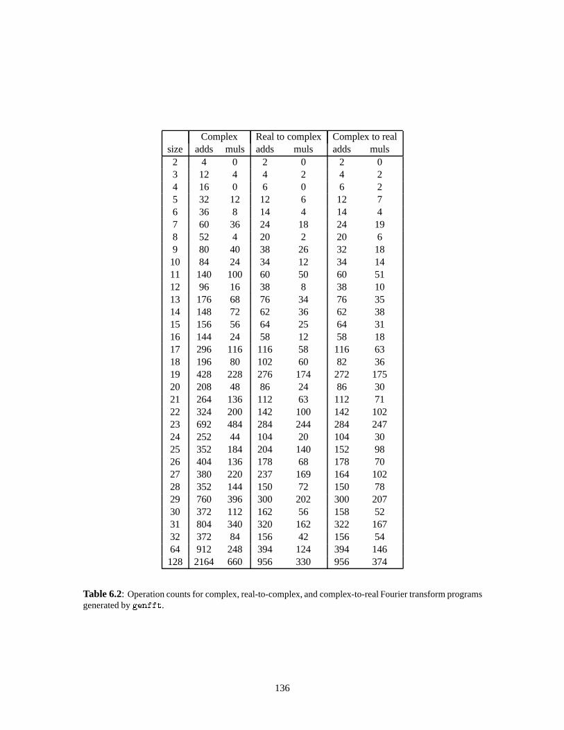
Complex Real to complex Complex to realsize adds muls adds muls adds muls2 4 0 2 0 2 03 12 4 4 2 4 24 16 0 6 0 6 25 32 12 12 6 12 76 36 8 14 4 14 47 60 36 24 18 24 198 52 4 20 2 20 69 80 40 38 26 32 1810 84 24 34 12 34 1411 140 100 60 50 60 5112 96 16 38 8 38 1013 176 68 76 34 76 3514 148 72 62 36 62 3815 156 56 64 25 64 3116 144 24 58 12 58 1817 296 116 116 58 116 6318 196 80 102 60 82 3619 428 228 276 174 272 17520 208 48 86 24 86 3021 264 136 112 63 112 7122 324 200 142 100 142 10223 692 484 284 244 284 24724 252 44 104 20 104 3025 352 184 204 140 152 9826 404 136 178 68 178 7027 380 220 237 169 164 10228 352 144 150 72 150 7829 760 396 300 202 300 20730 372 112 162 56 158 5231 804 340 320 162 322 16732 372 84 156 42 156 5464 912 248 394 124 394 146128 2164 660 956 330 956 374
Table 6.2: Operation counts for complex, real-to-complex, and complex-to-real Fourier transform programsgenerated bygenfft.
136

• Achieving correctnesshas been surprisingly easy. The DFT algorithms ingenfft are en-
coded straightforwardly using a high-level language. The simplification phase transforms
this high-level algorithm into optimized code by applying simple algebraic rules that are easy
to verify. In the rare cases during development when the generator contained a bug, the output
was completely incorrect, making the bug manifest.
• Rapid turnaroundwas essential to achieve the performance goals. Becausegenfft separates
the specificationof a DFT algorithm from itsimplementation, one can quickly experiment
with optimizations and determine their effect experimentally. For example, the minus-sign
propagation trick that we will describe in Section 6.6 could be implemented in only a few
lines of code and tested within minutes.
• The generator is effective because it can applyproblem-specificcode improvements. For
example, the scheduler is effective only for DFT dags, and it would perform poorly for other
computations. Moreover, the simplifier performs certain improvements that depend on the
DFT being a linear transformation.
• Finally, genfft derived somenew algorithms, as in the examplen = 13 discussed above.
While this dissertation does not focus on these algorithmsper se, they are of independent
theoretical and practical interest.
In the next three sections, we describe the operation ofgenfft. Section 6.5 shows howgenfft
creates a dag for a codelet. Section 6.6 describes howgenfft simplifies the dag. Section 6.7
describesgenfft’s cache-oblivious scheduler.
6.5 Creation of the expression dag
This section describes howgenfft creates an expression dag by evaluating a DFT algorithm sym-
bolically. Consistently with the metaprogramming philosophy of separating the algorithm with the
implementation, ingenfft we express DFT algorithms at a high level, almost “straight out of the
DSP book,” without worrying about optimization. This section first describes the data type that
encodes a codelet dag. Then, we show how the Cooley-Tukey algorithm (Equation (6.3)) translates
verbatim into Caml code.
We start by defining thenode data type, which encodes an arithmetic expression dag. Each
dag node represents an operator, and the node’s children represent the operands. This is the same
representation as the one generally used in compilers [9, Section 5.2]. A node in the dag can have
more than one “parent”, in which case the node represents a common subexpression. The Objective
Caml definition ofnode is given in Figure 6-15, and it is straightforward. A node is either a real
number (encoded by the abstract data typeNumber.number), a load of an input variable, a store of
137

type node =
| Num of Number.number
| Load of Variable.variable
| Store of Variable.variable * node
| Plus of node list
| Times of node * node
| Uminus of node
Figure 6-15: Objective Caml code that defines thenode data type, which encodes an expression dag.
an expression into an output node, the sum of the children nodes, the product of two nodes, or the
sign negation of a node. For example, the expressiona � b, wherea andb are input variables, is
represented byPlus [Load a; Uminus (Load b)].
The structureNumber maintains floating-point constants with arbitrarily high precision. FFTW
currently computes all constants with 50 decimal digits of precision, so that a user can use the
quadruple precision floating-point unit on a processor such as the UltraSPARC.Number is imple-
mented on top of Objective Caml’s arbitrary-precision rationals. If you wish, this is an extreme form
of portability: If machines with 100-digits floating-point accuracy ever become available, FFTW is
ready to run on them. The structureVariable encodes the input/output nodes of the dag, and the
temporary variables of the generated C code. For the purposes of this dissertation, variables can be
considered an abstract data type that is never used explicitly.
Thenode data type encodes expressions over real numbers, since the final C output contains
only real expressions. For creating the expression dag of the codelet, however, it is convenient
to express the algorithms in terms of complex numbers. The generator contains a structure called
Complex, which implements complex expressions on top of thenode data type, in a straightforward
way.7 The typeComplex.expr (not shown) is essentially a pair ofnodes.
We now describe the functionfftgen, which creates a dag for a DFT of sizen. In the current
implementation,fftgen uses one of the following algorithms.
• A split-radix algorithm [48], ifn is a multiple of4. Otherwise,
• A prime factor algorithm (as described in [121, page 619]), ifn factors inton1n2, where
ni 6= 1 andgcd(n1; n2) = 1. Otherwise,
• The Cooley-Tukey FFT algorithm (Equation (6.3)) ifn factors inton1n2, whereni 6= 1.
Otherwise,
7One subtlety is that a complex multiplication by a constant can be implemented with either 4 real multiplicationsand 2 real additions, or 3 real multiplications and 3 real additions [92, Exercise 4.6.4-41]. The current generator usesthe former algorithm, since the operation count of the dag is generally dominated by additions. On most CPUs, it isadvantageous to move work from the floating-point adder to the multiplier.
138

let rec cooley_tukey n1 n2 input sign =
let tmp1 j2 = fftgen n1
(fun j1 -> input (j1 * n2 + j2)) sign in
let tmp2 i1 j2 =
exp n (sign * i1 * j2) @* tmp1 j2 i1 in
let tmp3 i1 = fftgen n2 (tmp2 i1) sign
in
(fun i -> tmp3 (i mod n1) (i / n1))
Figure 6-16: Fragment of the FFTW codelet generator that implements the Cooley-Tukey FFT algo-rithm. The infix operator@* computes the complex product. The functionexp n k computes the constantexp(2�k
p�1=n).
• (n is a prime number) Rader’s algorithm for transforms of prime length [126] ifn = 5 or
n � 13. Otherwise,
• Direct application of the definition of DFT (Equation (6.1)).
We now look at the operation offftgen more closely. The function has type
fftgen : int -> (int -> Complex.expr) ->
int -> (int -> Complex.expr)
The first argument tofftgen is the sizen of the transform. The second argument is a function
input with typeint -> Complex.expr. The application(input i) returns a complex expres-
sion that contains thei-th input. The third argumentsign is either1 or �1, and it determines the
direction of the transform.
Depending on the sizen of the requested transform,fftgen dispatches one of the algorithms
mentioned above. We now discuss howgenfft implements the Cooley-Tukey FFT algorithm. The
implementation of the other algorithms proceeds along similar lines.
Objective Caml code that implements the Cooley-Tukey algorithm can be found in Figure 6-16.
In order to understand the code, recall Equation (6.3). This equation translates almost verbatim
into Objective Caml. With reference to Figure 6-16, the function applicationtmp1 j2 computes
the inner sum of Equation (6.3) for a given value ofj2, and it returns a function ofi1. (tmp1
is curried overi1, and thereforei1 does not appear explicitly in the definition.) Next,(tmp1 j2
i1) is multiplied by the twiddle factors, yieldingtmp2, that is, the expression in square braces in
Equation (6.3). Next,tmp3 computes the outer summation, which is itself a DFT of sizen2. (Again,
tmp3 is a function ofi1 andi2, curried overi2.) In order to obtain thei-th element of the output of
the transform, the indexi is finally mapped intoi1 andi2 and(tmp3 i1 i2) is returned.
Observe that the code in Figure 6-16 does not actually perform any computation. Instead, it
builds a symbolic expression dag that specifies the computation. The other DFT algorithms are
implemented in a similar fashion.
139

At the top level, the generator invokesfftgen with the sizen and the directionsign specified
by the user. Theinput function is set tofun i -> Complex.load (Variable.input i), i.e.,
a function that loads thei-th input variable. Recall now thatfftgen returns a functionoutput,
where(output i) is a complex expression that computes thei-th element of the output array. The
top level builds a list ofStore expressions that store(output i) into thei-th output variable, for
all 0 � i < n. This list ofStores is the codelet dag that forms the input of subsequent phases of
the generator.
We conclude this section with a some remarks. According to the description given in this sec-
tion, fftgen contains no special support for the case where the input is real. This statement is not
completely true. In the actual implementation,fftgen maintains certain symmetries explicitly. For
example, if the input is real, then the output is known to have hermitian symmetry. These addi-
tional constraints do not change the final output, but they speed up the generation process, since
they avoid computing and simplifying the same expression twice. For the same reason, the actual
implementation memoizes expressions such astmp1 i2 i1 in Figure 6-16, so that they are only
computed once. These performance improvements were important for a user of FFTW who needed
a hard-coded transform of size 101, and had not obtained an answer after the generator had run for
three days. (See Section 6.9 for more details on the running time ofgenfft.)
At this stage, the generated dag contains many redundant computations, such as multiplications
by 1 or 0, additions of0, and so forth.fftgen makes no attempt to eliminate these redundancies.
Figure 6-17 shows a possible C translation of a codelet dag at this stage of the generation process.
6.6 The simplifier
In this section, we presentgenfft’s simplifier, which transforms code such as the one in Fig-
ure 6-17 into simpler code. This section is divided into two parts. We first discuss how the simpli-
fier transforms the dag by applying algebraic transformations, common-subexpression elimination,
minus-sign propagation and network transposition. Then, we discuss the actual implementation of
the simplifier. Monads [151] form a convenient structuring mechanism for the code of the simplifier.
6.6.1 What the simplifier does
We begin by illustrating the improvements applied by the simplifier to a codelet dag. The simpli-
fier traverses the dag bottom-up, and it applies a series of local improvements to every node. For
explanation purposes, these improvements can be subdivided into three categories: algebraic trans-
formations, common-subexpression elimination, and DFT-specific improvements. Since the first
two kinds are well-known [9], I just discuss them briefly. We then consider the third kind in more
detail.
140

tmp1 = REAL(input[0]);
tmp5 = REAL(input[0]);
tmp6 = IMAG(input[0]);
tmp2 = IMAG(input[0]);
tmp3 = REAL(input[1]);
tmp7 = REAL(input[1]);
tmp8 = IMAG(input[1]);
tmp4 = IMAG(input[1]);
REAL(output[0]) = ((1 * tmp1) - (0 * tmp2))
+ ((1 * tmp3) - (0 * tmp4));
IMAG(output[0]) = ((1 * tmp2) + (0 * tmp1))
+ ((1 * tmp4) + (0 * tmp3));
REAL(output[1]) = ((1 * tmp5) - (0 * tmp6))
+ ((-1 * tmp7) - (0 * tmp8));
IMAG(output[1]) = ((1 * tmp6) + (0 * tmp5))
+ ((-1 * tmp8) + (0 * tmp7));
Figure 6-17: C translation of a dag for a complex DFT of size 2, as generated byfftgen. Variabledeclarations have been omitted from the figure. The code contains many common subexpression (e.g.,tmp1
andtmp5), and redundant multiplications by0 or 1.
Algebraic transformationsreduce the arithmetic complexity of the dag. Like a traditional com-
piler, the simplifier performs constant folding, and it simplifies multiplications by0, 1, or�1, and
additions of0. Moreover, the simplifier applies the distributive property systematically. Expres-
sions of the formkx+ ky are transformed intok(x+ y). In the same way, expressions of the form
k1x+k2x are transformed into(k1+k2)x. In general, these two transformations have the potential
of destroying common subexpressions, and they might increase the operation count. This does not
appear to be the case for all DFT dags I have studied, although I do not fully understand the reason
for this phenomenon.
Common-subexpression eliminationis also applied systematically. Not only does the simplifier
eliminate common subexpressions, it also attempts to create new ones. For example, it is common
for a DFT dag (especially in the case of real input) to contain bothx�y andy�x as subexpressions,
for somex andy. The simplifier converts both expressions to eitherx�y and�(x�y), or�(y�x)andy � x, depending on which expression is encountered first during the dag traversal.
The simplifier applies two kinds ofDFT-specific improvements. First, all numeric constants
are made positive, possibly propagating a minus sign to other nodes of the dag. This curious trans-
formation is effective because constants generally appear in pairsk and�k in a DFT dag. To my
knowledge, every C compiler would store bothk and�k in the program text, and it would load both
constants into a register at runtime. Making all constants positive reduces the number of loads of
constants by a factor of two, and this transformation alone speeds up the generated codelets by 10-
15% on most machines. This transformation has the additional effect of converting subexpressions
141

x
y
s
t4
5
3 2
�st
�=
�5 32 4
��xy
�
x
y
s
t4
5
3 2
�xy
�=
�5 23 4
��st
�
Figure 6-18: Illustration of “network” transposition. Each graph defines an algorithm for computing a linearfunction. These graphs are calledlinear networks, and they can be interpreted as follows. Data are flowingin the network, from input nodes to output nodes. An edge multiplies data by some constant (possibly1), andeach node is understood to compute the sum of all incoming edges. In this example, the network on the leftcomputess = 5x+3y andt = 2x+4y. The network on the right is the “transposed” form of the first network,obtained by reversing all edges. The new network computes the linear functionx = 5s+2t andy = 3s+4t.In general, if a network computesx =My for some matrixM , the transposed network computesy =MTx.(See [44] for a proof.) These linear networks are similar to but not the same as expression dags normally usedin compilers and ingenfft, because in the latter case the nodes and not the edges perform computation. Anetwork can be easily transformed into an expression dag, however. The converse is not true in general, butit is true for DFT dags where all multiplications are by constants.
into a canonical form, which helps common-subexpression elimination.
The second DFT-specific improvement is not local to nodes, and is instead applied to the whole
dag. The transformation is based on the fact that a dag computing a linear function can be “reversed”
yielding atransposeddag [44]. This transposition process is well-known in the Signal Processing
literature [121, page 309], and it operates a shown in Figure 6-18. It turns out that in certain
cases the transposed dag exposes some simplifications that are not present in the original dag. (An
example will be shown later.) Accordingly, the simplifier performs three passes over the dag. It first
simplifies the original dagG yielding a dagG1. Then, it simplifies the transposed dagGT1 yielding
a dagGT2 . Finally, it simplifiesG2 (the transposed dag ofGT
2 ) yielding a dagG3. (Although one
might imagine iterating this process, three passes seem to be sufficient in all cases.) Figure 6-19
shows the savings in arithmetic complexity that derive from network transposition for codelets of
various sizes. As it can be seen in the figure, transposition can reduce the number of multiplications,
but it does not reduce the number of additions.
Figure 6-20 shows a simple case where transposition is beneficial. The network in the figure
computesc = 4 � (2a + 3b). It is not safe to simplify this expression toc = 8a + 12b, since
this transformation destroys the common subexpressions2a and3b. (The transformation destroys 1
operation and 2 common subexpressions, which might increase the operation count by 1.) Indeed,
the whole point of most FFT algorithms is to create common subexpressions. When the network
is transposed, however, it computesa = 2 � 4c andb = 3 � 4c. These transposed expressionscan
be safely transformed intoa = 8c andb = 12c because each transformation saves 1 operation and
142
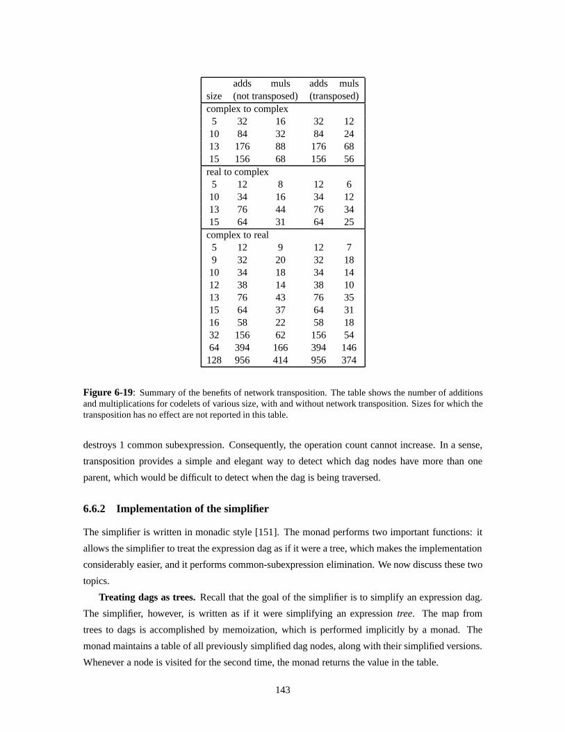
adds muls adds mulssize (not transposed) (transposed)complex to complex5 32 16 32 1210 84 32 84 2413 176 88 176 6815 156 68 156 56real to complex5 12 8 12 610 34 16 34 1213 76 44 76 3415 64 31 64 25complex to real5 12 9 12 79 32 20 32 1810 34 18 34 1412 38 14 38 1013 76 43 76 3515 64 37 64 3116 58 22 58 1832 156 62 156 5464 394 166 394 146128 956 414 956 374
Figure 6-19: Summary of the benefits of network transposition. The table shows the number of additionsand multiplications for codelets of various size, with and without network transposition. Sizes for which thetransposition has no effect are not reported in this table.
destroys 1 common subexpression. Consequently, the operation count cannot increase. In a sense,
transposition provides a simple and elegant way to detect which dag nodes have more than one
parent, which would be difficult to detect when the dag is being traversed.
6.6.2 Implementation of the simplifier
The simplifier is written in monadic style [151]. The monad performs two important functions: it
allows the simplifier to treat the expression dag as if it were a tree, which makes the implementation
considerably easier, and it performs common-subexpression elimination. We now discuss these two
topics.
Treating dags as trees.Recall that the goal of the simplifier is to simplify an expression dag.
The simplifier, however, is written as if it were simplifying an expressiontree. The map from
trees to dags is accomplished by memoization, which is performed implicitly by a monad. The
monad maintains a table of all previously simplified dag nodes, along with their simplified versions.
Whenever a node is visited for the second time, the monad returns the value in the table.
143
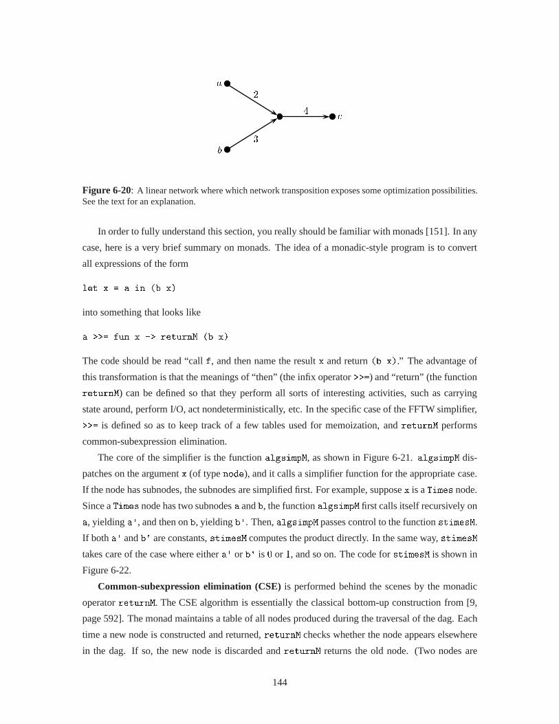
a
b
c4
2
3
Figure 6-20: A linear network where which network transposition exposes some optimization possibilities.See the text for an explanation.
In order to fully understand this section, you really should be familiar with monads [151]. In any
case, here is a very brief summary on monads. The idea of a monadic-style program is to convert
all expressions of the form
let x = a in (b x)
into something that looks like
a >>= fun x -> returnM (b x)
The code should be read “callf, and then name the resultx and return(b x).” The advantage of
this transformation is that the meanings of “then” (the infix operator>>=) and “return” (the function
returnM) can be defined so that they perform all sorts of interesting activities, such as carrying
state around, perform I/O, act nondeterministically, etc. In the specific case of the FFTW simplifier,
>>= is defined so as to keep track of a few tables used for memoization, andreturnM performs
common-subexpression elimination.
The core of the simplifier is the functionalgsimpM, as shown in Figure 6-21.algsimpM dis-
patches on the argumentx (of typenode), and it calls a simplifier function for the appropriate case.
If the node has subnodes, the subnodes are simplified first. For example, supposex is aTimes node.
Since aTimes node has two subnodesa andb, the functionalgsimpM first calls itself recursively on
a, yieldinga', and then onb, yieldingb'. Then,algsimpM passes control to the functionstimesM.
If both a' andb' are constants,stimesM computes the product directly. In the same way,stimesM
takes care of the case where eithera' or b' is 0 or 1, and so on. The code forstimesM is shown in
Figure 6-22.
Common-subexpression elimination (CSE)is performed behind the scenes by the monadic
operatorreturnM. The CSE algorithm is essentially the classical bottom-up construction from [9,
page 592]. The monad maintains a table of all nodes produced during the traversal of the dag. Each
time a new node is constructed and returned,returnM checks whether the node appears elsewhere
in the dag. If so, the new node is discarded andreturnM returns the old node. (Two nodes are
144

let rec algsimpM x =
memoizing
(function
Num a -> snumM a
| Plus a ->
mapM algsimpM a >>= splusM
| Times (a, b) ->
algsimpM a >>= fun a' ->
algsimpM b >>= fun b' ->
stimesM (a', b')
| Uminus a ->
algsimpM a >>= suminusM
| Store (v, a) ->
algsimpM a >>= fun a' ->
returnM (Store (v, a'))
| x -> returnM x)
x
Figure 6-21: The top-level simplifier functionalgsimpM, written in monadic style. See the text for anexplanation.
considered the same if they compute equivalent expressions. For example,a + b is the same as
b+ a.)
The simplifierinterleavescommon-subexpression elimination with algebraic transformations.
To see why interleaving is important, consider for example the expressiona � a0, wherea anda0
are distinct nodes of the dag that compute the same subexpression. CSE rewrites the expression to
a� a, which is then simplified to0. This pattern occurs frequently in DFT dags.
The idea of using memoization for graph traversal is very old, but monadic style provides a
particularly clean and modular implementation that isolates the memoization details. For example,
the operator>>= in Figures 6-21 and 6-22 performs one step of common-subexpression elimination
every time it is evaluated, it guarantees thatgenfft is not simplifying the same node twice, and so
on. When writing the simplifier, however, we need not be concerned with this bookkeeping, and we
can concentrate on the algebraic transformations that we want to implement.
6.7 The scheduler
In this section we discuss thegenfft “cache-oblivious” scheduler, which produces a topological
sort of the dag attempting to minimize register spills. For transforms whose size is a power of2,
genfft produces the cache-oblivious algorithm of Section 3.2, which is asymptotically optimal in
terms of register usage even though the schedule is independent of the number of registers.
Even after simplification, a codelet dag of a large transform typically contains hundreds or even
145
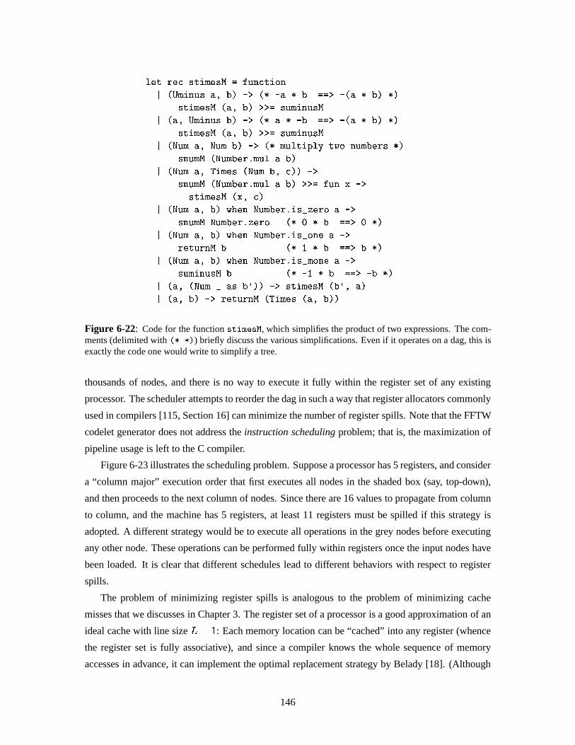
let rec stimesM = function
| (Uminus a, b) -> (* -a * b ==> -(a * b) *)
stimesM (a, b) >>= suminusM
| (a, Uminus b) -> (* a * -b ==> -(a * b) *)
stimesM (a, b) >>= suminusM
| (Num a, Num b) -> (* multiply two numbers *)
snumM (Number.mul a b)
| (Num a, Times (Num b, c)) ->
snumM (Number.mul a b) >>= fun x ->
stimesM (x, c)
| (Num a, b) when Number.is_zero a ->
snumM Number.zero (* 0 * b ==> 0 *)
| (Num a, b) when Number.is_one a ->
returnM b (* 1 * b ==> b *)
| (Num a, b) when Number.is_mone a ->
suminusM b (* -1 * b ==> -b *)
| (a, (Num _ as b')) -> stimesM (b', a)
| (a, b) -> returnM (Times (a, b))
Figure 6-22: Code for the functionstimesM, which simplifies the product of two expressions. The com-ments (delimited with(* *)) briefly discuss the various simplifications. Even if it operates on a dag, this isexactly the code one would write to simplify a tree.
thousands of nodes, and there is no way to execute it fully within the register set of any existing
processor. The scheduler attempts to reorder the dag in such a way that register allocators commonly
used in compilers [115, Section 16] can minimize the number of register spills. Note that the FFTW
codelet generator does not address theinstruction schedulingproblem; that is, the maximization of
pipeline usage is left to the C compiler.
Figure 6-23 illustrates the scheduling problem. Suppose a processor has 5 registers, and consider
a “column major” execution order that first executes all nodes in the shaded box (say, top-down),
and then proceeds to the next column of nodes. Since there are 16 values to propagate from column
to column, and the machine has 5 registers, at least 11 registers must be spilled if this strategy is
adopted. A different strategy would be to execute all operations in the grey nodes before executing
any other node. These operations can be performed fully within registers once the input nodes have
been loaded. It is clear that different schedules lead to different behaviors with respect to register
spills.
The problem of minimizing register spills is analogous to the problem of minimizing cache
misses that we discusses in Chapter 3. The register set of a processor is a good approximation of an
ideal cache with line sizeL = 1: Each memory location can be “cached” into any register (whence
the register set is fully associative), and since a compiler knows the whole sequence of memory
accesses in advance, it can implement the optimal replacement strategy by Belady [18]. (Although
146
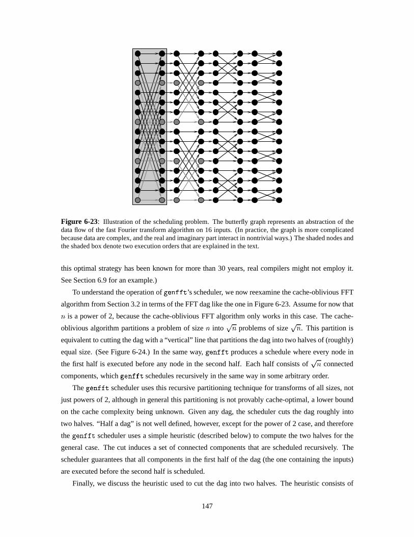
Figure 6-23: Illustration of the scheduling problem. The butterfly graph represents an abstraction of thedata flow of the fast Fourier transform algorithm on 16 inputs. (In practice, the graph is more complicatedbecause data are complex, and the real and imaginary part interact in nontrivial ways.) The shaded nodes andthe shaded box denote two execution orders that are explained in the text.
this optimal strategy has been known for more than 30 years, real compilers might not employ it.
See Section 6.9 for an example.)
To understand the operation ofgenfft’s scheduler, we now reexamine the cache-oblivious FFT
algorithm from Section 3.2 in terms of the FFT dag like the one in Figure 6-23. Assume for now that
n is a power of 2, because the cache-oblivious FFT algorithm only works in this case. The cache-
oblivious algorithm partitions a problem of sizen intopn problems of size
pn. This partition is
equivalent to cutting the dag with a “vertical” line that partitions the dag into two halves of (roughly)
equal size. (See Figure 6-24.) In the same way,genfft produces a schedule where every node in
the first half is executed before any node in the second half. Each half consists ofpn connected
components, whichgenfft schedules recursively in the same way in some arbitrary order.
Thegenfft scheduler uses this recursive partitioning technique for transforms of all sizes, not
just powers of 2, although in general this partitioning is not provably cache-optimal, a lower bound
on the cache complexity being unknown. Given any dag, the scheduler cuts the dag roughly into
two halves. “Half a dag” is not well defined, however, except for the power of 2 case, and therefore
thegenfft scheduler uses a simple heuristic (described below) to compute the two halves for the
general case. The cut induces a set of connected components that are scheduled recursively. The
scheduler guarantees that all components in the first half of the dag (the one containing the inputs)
are executed before the second half is scheduled.
Finally, we discuss the heuristic used to cut the dag into two halves. The heuristic consists of
147

Figure 6-24: Illustration of the recursive partitioning operated by thegenfft cache-oblivious scheduler.Like Figure 6-23, this figure shows the data flow dag of a FFT of 16 points. By cutting the dag in the“middle”, as determined by the dashed lines, we produce
p16 = 4 connected components on each side of
the cut. These components are shown in the figure with different shades of gray.
“burning the candle at both ends”. Initially, the scheduler colors the input nodes red, the output
nodes blue, and all other nodes black. After this initial step, the scheduler alternates between a red
and a blue coloring phase. In a red phase, any node whose predecessors are all red becomes red.
In a blue phase, all nodes whose successors are blue are colored blue. This alternation continues
while black nodes exist. When coloring is done, red nodes form the first “half” of the dag, and blue
nodes the second. Whenn is a power of 2, the FFT dag has a regular structure like the one shown
in Figure 6-24, and this process has the effect of cutting the dag in the middle with a vertical line,
yielding the desired optimal cache-oblivious behavior.
6.8 Real and multidimensional transforms
In this section, we discuss the implementation of real and multidimensional transforms in FFTW.
Like complex transforms, the real transform code uses “normal” and “twiddle” codelets, and it
employs its own planner and executor. The multidimensional code currently is built on top of one-
dimensional transforms, that is, FFTW does not use multidimensional codelets.
Real one-dimensional transforms. FFTW computes real transforms using a planner and an ex-
ecutor similar to those of complex transforms. The executor currently implements a real variant of
the Cooley-Tukey algorithm. Transforms of prime size are currently computed using Equation (6.1),
and not by Rader’s algorithm. Real input data occur frequently in applications, and a specialized
148
real DFT code is important because the transform of a real array is an array with hermitian sym-
metry. Because of this symmetry, half of the output array is redundant and need not be computed
and stored. Real transforms introduce two complications, however. First, hermitian arrays must be
stored in such a way that the Cooley-Tukey recursion can be executed without performing compli-
cated permutations. Second, the inverse transform can no longer be computed by conjugation of
certain constants, because the input to the inverse transform is a hermitian array (as opposed to a
real array) and the output is real (as opposed to hermitian).
FFTW stores a hermitian arrayX[0 : : : n�1] into a real arrayY [0 : : : n�1] using the following
halfcomplexstorage layout. For all integersi such that0 � i � bn=2c, we haveY [i] = Re(X[i]).
For all integersi such that0 < i < bn=2c, we haveY [n � i] := Im(X[i]). In other words, if
rj = Re(X[j]) andij = Im(X[j]), the arrayY has the form:
r0; r1; r2; : : : ; rbn=2c; ib(n�1)=2c; : : : ; i2; i1 :
This layout is a generalization of the layout presented in [136]. The name “halfcomplex” appears
in the GNU Scientific Library (GSL)[59], which uses this layout for powers-of-2 transforms. This
storage scheme is useful becausen1 halfcomplex arrays, each containing a transform of sizen2,
can be combined in place to produce a transform of sizen1n2, just like in the complex case. This
property is not true of layouts like the one used in FFTPACK [139], which stores a hermitian array
by interleaving real and imaginary parts as follows.
Hence, the FFTW forward real executor is recursive and it contains two kinds of codelets.Real-
to-halfcomplexcodelets form the leaves of the recursion. Their input is a real array, and their
output is the DFT of the input in halfcomplex order.Forward halfcomplexcodelets combine small
transforms (in halfcomplex order) to produce a larger transform. Similarly, the backward real ex-
ecutor useshalfcomplex-to-realcodelets at the leaves of the recursion, andbackward halfcomplex
codelets in the intermediate stages. A backward halfcomplex codelet splits a large halfcomplex
array into smaller arrays, that are then transformed recursively.
Multidimensional transforms. Multidimensional transforms are currently implemented on top
of one-dimensional transforms. For example, a two-dimensional DFT of an array is computed by
transforming all rows and then all columns (or vice versa). Alternatively, and more in the spirit of
the rest of the FFTW system, we could use multidimensional codelets. For example, in the 2D case,
we could employ two-dimensional codelets to “tile” the array. While it would be easy to modify
genfft to produce the required codelets, this approach leads to an explosion in code size that is
currently unacceptable, and the performance gains do not appear to justify the effort. This tradeoff
will probably change once computers have so much memory that codelet size is not a problem. One
drawback of the current implementation is that it is inefficient for small transforms. For example,
149

on most processors it would be much faster to compute a4� 4 transform with a special codelet.
6.9 Pragmatic aspects of FFTW
This section discusses briefly the running time and the memory requirements ofgenfft, some
problems that arise in the interaction of thegenfft scheduler with C compilers, and FFTW’s testing
methodology.
Resource requirements. The FFTW codelet generator is not optimized for speed, since it is in-
tended to be run only once. Indeed, users of FFTW can download a distribution of generated C
code and never rungenfft at all. Nevertheless, the resources needed bygenfft are quite modest.
Generation of C code for a transform of size 64 (the biggest used in FFTW) takes about 75 seconds
on a 200MHz Pentium Pro running Linux 2.2 and the native-code compiler of Objective Caml 2.01.
genfft needs less than 3 MB of memory to complete the generation. The resulting codelet contains
912 additions, 248 multiplications. On the same machine, the whole FFTW system can be regener-
ated in about 15 minutes. The system contains about 55,000 lines of code in 120 files, consisting of
various kinds of codelets for forward, backward, real to complex, and complex to real transforms.
The sizes of these transforms in the standard FFTW distribution include all integers up to 16 and all
powers of 2 up to 64.
A few FFTW users needed fast hard-coded transforms of uncommon sizes (such as 19 and 23),
and they were able to run the generator to produce a system tailored to their needs. The biggest
program generated so far was for a complex transform of size 101, which required slightly less than
two hours of CPU time on the Pentium Pro machine, and about 10 MB of memory. Again, a user
had a special need for such a transform, which would be formidable to code by hand. In order to
achieve this running time, I was forced to replace a linked-list implementation of associative tables
by hashing, and to avoid generating “obvious” common subexpressions more than once when the
dag is created. The naive generator was somewhat more elegant, but had not produced an answer
after three days.
Interaction with C compilers. The long sequences of straight-line code produced bygenfft can
push C compilers (in particular, register allocators) to their limits. The combined effect ofgenfft
and of the C compiler can lead to performance problems. The following discussion presents two
particular cases that I found particularly surprising, and is not intended to blame any particular
compiler or vendor.
The optimizer of theegcs-1.1.1 compiler performs an instruction scheduling pass, followed
by register allocation, followed by another instruction scheduling pass. On some architectures,
including the SPARC and PowerPC processors,egcs employs the so-called “Haifa scheduler”,
150

void foo(void)
void foo(void) {
{ {
double a; double a;
double b; .. lifetime of a ..
}
.. lifetime of a .. {
.. lifetime of b .. double b;
} .. lifetime of b ..
}
}
Figure 6-25: Two possible declarations of local variables in C. On the left side, variables are declared in thetopmost lexical scope. On the right side, variables are declared in a private lexical scope that encompassesthe lifetime of the variable.
which usually produces better code than the normalegcs/gcc scheduler. The first pass of the
Haifa scheduler, however, has the unfortunate effect of destroyinggenfft’s schedule (computed as
explained in Section 6.7). Inegcs, the first instruction scheduling pass can be disabled with the
option-fno-schedule-insns, and on a 167-MHz UltraSPARC I, the compiled code is between
50% and 100% faster and about half the size when this option is used. Inspection of the assembly
code produced byegcs reveals that the difference consists entirely of register spills and reloads.
Digital’s C compiler for Alpha (DEC C V5.6-071 on Digital UNIX V4.0 (Rev. 878)) seems to
be particularly sensitive to the way local variables are declared. For example, Figure 6-25 illustrates
two ways to declare temporary variables in a C program. Let’s call them the “left” and the “right”
style. genfft can be programmed to produce code in either way, and for most compilers I have
tried there is no appreciable performance difference between the two styles. Digital’s C compiler,
however, appears to produce better code with the right style (the right side of Figure 6-25). For a
transform of size 64, for example, and compiler flags-newc -w0 -O5 -ansi alias -ansi args
-fp reorder -tune host -std1, a 467MHz Alpha achieves about 450 MFLOPS with the left
style, and 600 MFLOPS with the right style. (Different sizes lead to similar results.) I could not
determine the exact source of this difference.
Testing FFTW. FFTW uses different plans on each platform, and some codelets are not used at
all on the machines available to me. How do we ensure that FFTW is correct? FFTW uses the
self-testingalgorithm by Funda Erg¨un [49], a randomized test that guarantees that a given program
computes the DFT for an overwhelmingly large fraction of all possible inputs. The self-tester does
not require any other DFT program to be available. In the past, we checked FFTW against the pro-
gram by Singleton [132], assuming that any bug in the program would have been found in the thirty
years passed since the program was written. Unfortunately, while Singleton’s routine is correct, one
151
of the FORTRAN compilers we used was not. Besides, Singleton’s program does not work for all
input sizes, while FFTW does, and thus we could not test FFTW fully. In contrast, Erg¨un’s tester
is fast, easy to code, and it works for all sizes. Computer theoreticians have developed many test-
ing techniques that possess similar advantages, but regrettably, these techniques seem to be mostly
unknown to practitioners. I definitely recommend that any programmer become familiar with this
beautiful topic; see [24] for a gentle introduction.
6.10 Related work
Other systems exist with self-optimization capabilities. PHiPAC [22] generates automatically-tuned
matrix-multiplication kernels by generating many C programs and selecting the fastest. In most
cases, PHiPAC is able to beat hand-optimized BLAS routines. PHiPAC predates FFTW [21], but I
became acquainted with it only after the publication of [22] in July 1997, after the release of FFTW-
1.0 in March 1997. PhiPAC and FFTW focus on complementary aspects of self-optimization.
PHiPAC automatically optimizes the multiplication kernels, which correspond to FFTW’s codelets,
while FFTW optimizes compositions of codelets, or plans, and it relies ongenfft to produce good
codelets. Consequently, FFTW’s self-optimization occurs at runtime, while PHiPAC operates at
installation time and it is not needed after the kernels have been generated. Because of the mathe-
matical richness of the Fourier transform, FFTW employs a sophisticated compiler that focuses on
algebraic transformations and on cache-oblivious scheduling. On the other hand, PHiPAC uses the
standard matrix multiplication algorithm, and it is concerned with scheduling it appropriately for
a processor’s pipeline. Both approaches are legitimate and effective techniques for portable high
performance, and I expect FFTW to evolve to produce codelets tailored to a single machine, in the
same spirit of PHiPAC.
The Linux kernel included in Redhat 6.0 incorporates many routines that compute checksums
in the RAID disk drivers. At boot time, the kernel measures the execution time of the various
subroutines and uses the fastest.
Researchers have been generating FFT programs for at least twenty years, possibly to avoid the
tedium of getting all the implementation details right by hand. To my knowledge, the first generator
of FFT programs was FOURGEN, written by J. A. Maruhn [108]. It was written in PL/I and it
generated FORTRAN.8 FOURGEN is limited to transforms of size2k.
Perez and Takaoka [123] present a generator of Pascal programs implementing a prime factor
8Maruhn argues that PL/I is more suited than FORTRAN to this program-generation task, and has the followingcurious remark:
One peculiar difficulty is that some FORTRAN systems produce an output format for floating-point num-bers without the exponent delimiter “E”, and this makes them illegal in FORTRAN statements.
152

FFT algorithm. This program is limited to complex transforms of sizen, wherenmust be factorable
into mutually prime factors in the setf2; 3; 4; 5; 7; 8; 9; 16g.Johnson9 and Burrus [86] applied dynamic programming to the automatic design of DFT mod-
ules. Selesnick and Burrus [131] used a program to generate MATLAB subroutines for DFT’s of
certain prime sizes. In many cases, these subroutines are the best known in terms of arithmetic
complexity.
The EXTENT system by Gupta and others [74] generates FORTRAN code in response to an
input expressed in atensor productlanguage. Using the tensor product abstraction one can ex-
press concisely a variety of algorithms that includes the FFT and matrix multiplication (including
Strassen’s algorithm).
Another program calledgenfft generating Haskell FFT subroutines is part of thenofib bench-
mark for Haskell [122]. Unlike my program, thisgenfft is limited to transforms of size2k. The
program innofib is not documented at all, but apparently it can be traced back to [77].
Veldhuizen [146] used a template metaprograms technique to generateC++ programs. The
technique exploits the template facility ofC++ to force theC++ compiler to perform computations
at compile time.
All these code generators are restricted to complex transforms, and the FFT algorithm is known
a priori. To my knowledge, the FFTW generator is the only one that produces real algorithms, and
in fact, which canderivereal algorithms by specializing a complex algorithm. Also, my generator
is the only one that addressed the problem of scheduling the program efficiently.
6.11 Conclusion
Current computer systems are so complex that their behavior is unpredictable. Ironically, while
performance is the very reason for this complexity, peak performance is almost impossible to at-
tain because of lack of predictability. Only time will tell whether we will regret having designed
machines so complex. In the meanwhile, in this chapter we showed that a software system that is
aware of its own performance can achieve high performance with no tuning. For the case of FFTW,
a special-purpose compiler is a necessary component of such a self-optimizing system, because we
need a sufficiently large space of algorithmic variations to be able to pick the most effective.
From another point of view, this chapter presented a real-world application of domain-specific
compilers and of advanced programming techniques, such as monads. In this respect, the FFTW
experience has been very successful: the current release FFTW-2.1.2 is being downloaded by more
than 100 people every week, and a few users have been motivated to learn ML after their experience
with FFTW. In the rest of this concluding section, I offer some ideas about future work and possible
9Unrelated to Steven G. Johnson, the other author of FFTW.
153

developments of the FFTW system.
The currentgenfft program is somewhat specialized to computing linear functions, using al-
gorithms whose control structure is independent of the input. Even with this restriction, the field of
applicability ofgenfft is potentially huge. For example, signal processing FIR and IIR filters fall
into this category, as well as other kinds of transforms used in image processing (for example, the
discrete cosine transform used in JPEG). I am confident that the techniques described in this chapter
will prove valuable in this sort of application.
Recently, I modifiedgenfft to generate crystallographic Fourier transforms [12]. In this par-
ticular application, the input consists of 2D or 3D data with certain symmetries. For example, the
input data set might be invariant with respect to rotations of 60 degrees, and it is desirable to have
a special-purpose FFT algorithm that does not execute redundant computations. Preliminary in-
vestigation shows thatgenfft is able to exploit most symmetries. I am currently working on this
problem.
In its present form,genfft is somewhat unsatisfactory because it intermixes programming and
metaprogramming. At the programming level, one specifies a DFT algorithm, as in Figure 6-16.
At the metaprogramming level, one specifies how the program should be simplified and scheduled.
In the current implementation, the two levels are confused together in a single binary program. It
would be nice to build a general-purpose “metacompiler” that clearly separates programming from
metaprogramming and allows other problems to be addressed in a similar fashion.
154

Chapter 7
Conclusion
[T]here ain't nothing more to write about, and I
am rotten glad of it, because if I'd a knowed what
a trouble it was to make a book I wouldn't
a tackled it and aint't agoing to no more.
(Huckleberry Finn)
In this concluding chapter, we look at some ideas for future work, and we finally summarize the
main ideas of this thesis.
7.1 Future work
Portable high-performance I/O. The topic of portable high-performance disk I/O was not ad-
dressed at all in this document. We can identify two general research topics in this area, roughly
inspired by cache-oblivious algorithms and Cilk. The first topic is to design “disk-geometry-
oblivious” data structures for single (i.e., not parallel) disks. The second topic is to extend the
Cilk model with provably efficient parallel I/O.
Disk access time depends on the geometrical and mechanical properties of disks. Current disks
are partitioned intocylinders, and cylinders are divided intosectors. Data within the same sector
can be accessed quickly with one operation. Accesses within the same cylinder are slower than
accesses within a sector, but faster than accesses to another cylinder. In this latter case, the speed
of intra-cylinder accesses depends on the physical distance between the old and the new cylinder.
With current technology, the number of sectors per cylinder is not constant, since cylinders in the
outer part of the disk comprise a larger area and thus can host more sectors.
It should be possible to design “cache-oblivious” data structures to store data on a disk. Suppose
for example that we want to store a binary search tree on a disk. If a disk “cache line” (the unit of
155

transfer between disk and memory, usually called apageor a block) containsL elements, it is a
good idea to group subtrees of heightlgL, as explained in [91], so that a tree ofn elements can be
searched inlogL n page accesses. This disk-aware layout depends onL, but it is possible to devise
a “disk-oblivious” tree layout by cutting the tree at level(lg n)=2 and storing the resulting�(pn)
subtrees in a recursive fashion. This “disk-oblivious” layout has the same asymptotic I/O complexity
as the disk-aware one. I conjecture that this layout is insensitive to the variable number of sectors
per cylinder; if true, this conjecture would show a nice advantage of cache-oblivious algorithms
over cache-aware ones. The ideal-cache theory does not model the intra-cylinder physical distance,
however. Is there a “disk-oblivious” way to store a binary tree on disk so as to minimize the total
execution time of the search, no matter what the parameters of the disk are? Indeed, the whole
topic of cache- and disk-oblivious data structures has not been investigated yet, and I would expect
such an investigation to yield useful algorithms and programming paradigms. For example, can we
design a cache/disk-oblivious B-tree?
Concerning parallel I/O, it would be nice to extend the Cilk system with I/O in a way that pre-
serves Cilk’s performance guarantees. Since files can be used to simulate shared memory, I expect
the solution to this problem to depend on the consistency model that we use for files. Location
consistency and other traditional memory models seem inadequate for the case of files, however.
For example, the “parallel append” file operation appears to be useful. In a parallel append, a file is
opened and two parallel threads are spawned to append data to the file. The output is the same as
if the C elision of the Cilk program had been executed, regardless of how many processors execute
the parallel program. How to implement parallel append preserving the performance of the Cilk
scheduler is an open problem.
Extensions to Cilk. The Cilk system needs to be extended to support other kinds of synchroniza-
tion, such as producer-consumer relationships and mutual exclusion. Currently, the Cilk-5 imple-
mentation of locks is an afterthought that invalidates many of Cilk’s performance guarantees. Even
worse, there is no linguistic support for locks in Cilk (the Nondeterminator will detect data races in
programs that use locks [37], however). How to incorporate easy-to-use and efficient synchroniza-
tion in a general-purpose programming language is a tough problem that nobody has fully solved
yet. If you find a solution, submit it immediately to the Java and Perl authors before the World-Wide
Web collapses because of incorrect protocols.
From the point of view of the Cilk implementation, Cilk needs work in two directions. First,
Cilk for SMP’s should be made easily available to the general public. Although every version of
Cilk has been publicly released, and although Cilk-5 is relatively bug-free and robust, the system
is still a research prototype. Cilk is mature enough to become a “product,” and it is time to write a
production-quality system, which should be distributed with Linux and other operating systems so
that many people can use it. Second, Cilk needs to be implemented on distributed-memory systems
156

such as networks of workstations. An implementation was written by Keith Randall [127] for Unix
systems, but this implementation is still preliminary. The main problem is the implementation of
shared memory, using BACKER or its variants described in [127]. Keith’s implementation uses the
Unix user-level virtual-memory system, but this solution is too slow. It seems necessary to imple-
ment BACKER in the Unix kernel, where it can use the virtual-memory and network subsystems
without too many overheads. Fortunately, the Linux kernel is currently robust and mature enough
that such an implementation is feasible and will probably be efficient.
Extensions to FFTW. The current FFTW system covers most of the spectrum of practical uses of
Fourier transforms, but it would be nice to extend it to compute related transforms, such as the dis-
crete cosine transform (DCT) and maybe the Hartley transform [31]. Currently,genfft is capable
of generating DCT programs, but the planner/executor machinery has not been implemented.
We should implement a planner for multidimensional transforms and an executor that uses mul-
tidimensional codelets. I expect performance improvements at least for small transforms (say,
4 � 4 � 4 or 8 � 8), which can be unrolled as straight-line code. The8 � 8 DCT is especially
important because it is used in the JPEG image compression standard.
Open problems in cache-obliviousness. The limits of cache obliviousness need to be investi-
gated. In particular, it is unknown whether the cache complexity of cache-aware algorithms is
inherently lower than the complexity of cache-oblivious algorithms. It would be nice to find a
separation between the two classes, as well as a simulation result that shows how to make any
cache-aware algorithm cache-oblivious with minimal increase in its cache complexity.
Compiler research. The work of this dissertation inspires two lines of research in compilers.
First, because divide and conquer is such an important technique in portable high-performance
programs, we should investigate compiler techniques to unroll recursion, in the same way as current
compilers unroll loops.
Second, the FFTW system shows the importance of metaprogramming for high performance,
whether it be portable or not. For example, the fastest code for a DFT of size 64 on an Alpha
processor is one of FFTW’s codelets, which consists of about 2400 lines of code. It would have
been very hard to write this code by hand. We should investigate the general idea of ametacompiler,
which allows a programmer to write both a program and a metaprogram as done ingenfft. The
programmer should be allowed to express algorithms at a high level, and specify how he or she
wants the program to be compiled. I do not expect such a system to be generally applicable, but
genfft shows that even if the metacompiler works for only one problem, it is still worth the effort.
157

7.2 Summary
In this dissertation we explored techniques to write fast programs whose high-performance is portable
in the face of parallelism, memory hierarchy, and diverse processor architectures.
To write high-performance parallel programs, we developed the Cilk-5 language and system.
Cilk provides simple yet powerful constructs for expressing parallelism in an application. Cilk
programs run on one processor as efficiently as equivalent sequential programs, and they scale up
on multiple processors. Cilk’s compilation and runtime strategies, which are inspired by the “work-
first principle,” are effective for writing portable high-performance parallel programs.
Cache-oblivious algorithms provide performance and portability across platforms with different
cache sizes. They are oblivious to the parameters of the memory hierarchy, and yet they use multiple
levels of caches asymptotically optimally. In this dissertation, we discussed cache-oblivious algo-
rithms for matrix transpose and multiplication, FFT, and sorting that are asymptotically as good as
previously known cache-aware algorithms, and provably optimal for those problems whose optimal
cache complexity is known.
The location consistency memory model and the BACKER coherence algorithm are one way
to achieve portability in high-performance parallel systems with a memory hierarchy. In this dis-
sertation, we proved good asymptotic performance bounds for Cilk programs that uses location
consistency.
Finally, the FFTW library adapts itself to the hardware, and it deals automatically with some of
the intricacies of processor architectures. While FFTW does not require machine-specific perfor-
mance tuning, its performance is comparable with or better than codes that were tuned for specific
machines.
158
Bibliography
[1] S. ADVE AND K. GHARACHORLOO, Shared memory consistency models: A tutorial, Tech.Rep. 9512, Rice University, Sept. 1995.http://www-ece.rice.edu/ece/faculty/Adve/publications/models tutorial.ps.
[2] S. V. ADVE AND K. GHARACHORLOO, Shared memory consistency models: A tutorial,IEEE Computer, (1996), pp. 66–76.
[3] S. V. ADVE AND M. D. HILL , Weak ordering - new definition, in Proceedings of the 17thAnnual International Symposium on Computer Architecture, Seattle, Washington, May 1990,pp. 2–14.
[4] A. A GGARWAL, B. ALPERN, A. K. CHANDRA, AND M. SNIR, A model for hierarchicalmemory, in Proceedings of the 19th Annual ACM Symposium on Theory of Computing, May1987, pp. 305–314.
[5] A. A GGARWAL, A. K. CHANDRA, AND M. SNIR, Hierarchical memory with block transfer,in 28th Annual Symposium on Foundations of Computer Science, Los Angeles, California,12–14 Oct. 1987, IEEE, pp. 204–216.
[6] A. A GGARWAL AND J. S. VITTER, The input/output complexity of sorting and related prob-lems, Communications of the ACM, 31 (1988), pp. 1116–1127.
[7] M. A HAMAD , P. W. HUTTO, AND R. JOHN, Implementing and programming causal dis-tributed shared memory, in Proceedings of the 11th International Conference on DistributedComputing systems, Arlington, Texas, May 1991, pp. 274–281.
[8] A. V. A HO, J. E. HOPCROFT, AND J. D. ULLMAN , The Design and Analysis of ComputerAlgorithms, Addison-Wesley Publishing Company, 1974.
[9] A. V. A HO, R. SETHI, AND J. D. ULLMAN , Compilers, principles, techniques, and tools,Addison-Wesley, Mar. 1986.
[10] S. G. AKL AND N. SANTORO, Optimal parallel merging and sorting without memory con-flicts, IEEE Transactions on Computers, C-36 (1987).
[11] B. ALPERN, L. CARTER, AND E. FEIG, Uniform memory hierarchies, in Proceedings of the31st Annual IEEE Symposium on Foundations of Computer Science, Oct. 1990, pp. 600–608.
[12] M. A N, J. W. COOLEY, AND R. TOLIMIERI , Factorization method for crystallographicFourier transforms, Advances in Applied Mathematics, 11 (1990), pp. 358–371.
159

[13] A. W. APPEL AND Z. SHAO, Empirical and analytic study of stack versus heap cost forlanguages with closures, Journal of Functional Programming, 6 (1996), pp. 47–74.
[14] N. S. ARORA, R. D. BLUMOFE, AND C. G. PLAXTON, Thread scheduling for multipro-grammed multiprocessors, in Proceedings of the Tenth Annual ACM Symposium on ParallelAlgorithms and Architectures (SPAA), Puerto Vallarta, Mexico, June 1998.
[15] ARVIND, Personal communication, Jan. 1998.
[16] ARVIND, J. W. MAESSEN, R. S. NIKHIL , AND J. STOY, Lambda-S: an implicitly parallellambda-calculus with letrec, synchronization and side-effects, tech. rep., MIT Laboratory forComputer Science, Nov 1996. Computation Structures Group Memo 393, also available athttp://www.csg.lcs.mit.edu:8001/pubs/csgmemo.html.
[17] D. H. BAILEY , FFTs in external or hierarchical memory, Journal of Supercomputing, 4(1990), pp. 23–35.
[18] L. A. BELADY, A study of replacement algorithms for virtual storage computers, IBM Sys-tems Journal, 5 (1966), pp. 78–101.
[19] M. BELTRAMETTI, K. BOBEY, AND J. R. ZORBAS, The control mechanism for the Myriasparallel computer system, Computer Architecture News, 16 (1988), pp. 21–30.
[20] B. N. BERSHAD, M. J. ZEKAUSKAS, AND W. A. SAWDON, The Midway distributed sharedmemory system, in Digest of Papers from the Thirty-Eighth IEEE Computer Society Interna-tional Conference (Spring COMPCON), San Francisco, California, Feb. 1993, pp. 528–537.
[21] J. BILMES, K. ASANOVIC, J. DEMMEL, D. LAM , AND C. CHIN, PHiPAC: A portable,high-performance, ANSI C coding methodology and its application to matrix multiply, LA-PACK working note 111, University of Tennessee, 1996.
[22] J. BILMES, K. ASANOVIC, C. WHYE CHIN, AND J. DEMMEL, Optimizing matrix multiplyusing PHiPAC: a portable, high-performance, ANSI C coding methodology, in Proceedingsof International Conference on Supercomputing, Vienna, Austria, July 1997.
[23] G. E. BLELLOCH, Programming parallel algorithms, Communications of the ACM, 39(1996), pp. 85–97.
[24] M. BLUM AND H. WASSERMAN, Reflections on the pentium bug, IEEE Transactions onComputers, 45 (1996), pp. 385–393.
[25] R. D. BLUMOFE, Executing Multithreaded Programs Efficiently, PhD thesis, Departmentof Electrical Engineering and Computer Science, Massachusetts Institute of Technology,September 1995.
[26] R. D. BLUMOFE, M. FRIGO, C. F. JOERG, C. E. LEISERSON, AND K. H. RANDALL ,An analysis of dag-consistent distributed shared-memory algorithms, in Proceedings of theEighth Annual ACM Symposium on Parallel Algorithms and Architectures (SPAA), Padua,Italy, June 1996, pp. 297–308.
[27] R. D. BLUMOFE, M. FRIGO, C. F. JOERG, C. E. LEISERSON, AND K. H. RANDALL ,Dag-consistent distributed shared memory, in Proceedings of the 10th International ParallelProcessing Symposium, Honolulu, Hawaii, Apr. 1996.
160
[28] R. D. BLUMOFE, C. F. JOERG, B. C. KUSZMAUL, C. E. LEISERSON, K. H. RANDALL ,AND Y. ZHOU, Cilk: An efficient multithreaded runtime system, in Proceedings of the FifthACM SIGPLAN Symposium on Principles and Practice of Parallel Programming (PPoPP),Santa Barbara, California, July 1995, pp. 207–216.
[29] , Cilk: An efficient multithreaded runtime system, Journal of Parallel and DistributedComputing, 37 (1996), pp. 55–69.
[30] R. D. BLUMOFE AND C. E. LEISERSON, Scheduling multithreaded computations by workstealing, in Proceedings of the 35th Annual Symposium on Foundations of Computer Sci-ence, Santa Fe, New Mexico, Nov. 1994, pp. 356–368.
[31] R. N. BRACEWELL, The Hartley Transform, Oxford Press, 1986.
[32] R. P. BRENT, The parallel evaluation of general arithmetic expressions, Journal of the ACM,21 (1974), pp. 201–206.
[33] J. B. CARTER, J. K. BENNETT, AND W. ZWAENEPOEL, Implementation and performanceof Munin, in Proceedings of the Thirteenth ACM Symposium on Operating Systems Princi-ples, Pacific Grove, California, Oct. 1991, pp. 152–164.
[34] B. L. CHAMBERLAIN , S.-E. CHOI, E. C. LEWIS, C. LIN, L. SNYDER, AND W. D.WEATHERSBY, The case for high level parallel programmin in zpl, IEEE ComputationalScience and Engineering, 5 (1998), pp. 76–86.
[35] S. CHATTERJEE, V. V. JAIN , A. R. LEBECK, AND S. MUNDHRA, Nonlinear array layoutsfor hierarchical memory systems, in Proceedings of the ACM International Conference onSupercomputing, Rhodes, Greece, June 1999.
[36] S. CHATTERJEE, A. R. LEBECK, P. K. PATNALA , AND M. THOTTETHODI, Recursive ar-ray layouts and fast parallel matrix multiplication, in Proceedings of the Eleventh ACMSIGPLAN Symposium on Parallel Algorithms and Architectures, June 1999.
[37] G.-I. CHENG, M. FENG, C. E. LEISERSON, K. H. RANDALL , AND A. F. STARK, Detect-ing data races in Cilk programs that use locks, in Proceedings of the Tenth Annual ACMSymposium on Parallel Algorithms and Architectures (SPAA), Puerto Vallarta, Mexico, June1998.
[38] Cilk-5.2 Reference Manual, 1998. Available on the Internet fromhttp://theory.lcs.mit.edu/~cilk.
[39] D. COMMITTEE, ed.,Programs for Digital Signal Processing, IEEE Press, 1979.
[40] J. W. COOLEY, P. A. W. LEWIS, AND P. D. WELCH, The Fast Fourier Transform algorithmand its applications, IBM Research, (1967).
[41] J. W. COOLEY AND J. W. TUKEY, An algorithm for the machine computation of the complexFourier series, Mathematics of Computation, 19 (1965), pp. 297–301.
[42] T. H. CORMEN, C. E. LEISERSON, AND R. L. RIVEST, Introduction to Algorithms, TheMIT Press, Cambridge, Massachusetts, 1990.
[43] R. E. CRANDALL AND B. FAGIN, Discrete weighted transforms and large-integer arith-metic, Math. Comp., (1994), pp. 305–324.
161
[44] R. E. CROCHIERE ANDA. V. OPPENHEIM, Analysis of linear digital networks, Proceedingsof the IEEE, 63 (1975), pp. 581–595.
[45] D. E. CULLER, A. SAH, K. E. SCHAUSER, T. VON EICKEN, AND J. WAWRZYNEK, Fine-grain parallelism with minimal hardware support: A compiler-controlled threaded abstractmachine, in Proceedings of the Fourth International Conference on Architectural Supportfor Programming Languages and Operating Systems, Santa Clara, California, Apr. 1991,pp. 164–175.
[46] E. W. DIJKSTRA, Solution of a problem in concurrent programming control, Communica-tions of the ACM, 8 (1965), p. 569.
[47] M. DUBOIS, C. SCHEURICH, AND F. A. BRIGGS, Memory access buffering in multiproces-sors, in Proceedings of the 13th Annual International Symposium on Computer Architecture,June 1986, pp. 434–442.
[48] P. DUHAMEL AND M. V ETTERLI, Fast Fourier transforms: a tutorial review and a state ofthe art, Signal Processing, 19 (1990), pp. 259–299.
[49] F. ERGUN, Testing multivariate linear functions: Overcoming the generator bottleneck, inProceedings of the Twenty-Seventh Annual ACM Symposium on the Theory of Computing,Las Vegas, Nevada, jun 1995, pp. 407–416.
[50] M. FEELEY, Polling efficiently on stock hardware, in Proceedings of the 1993 ACM SIG-PLAN Conference on Functional Programming and Computer Architecture, Copenhagen,Denmark, June 1993, pp. 179–187.
[51] S. I. FELDMAN , D. M. GAY, M. W. MAIMONE, AND N. L. SCHRYER, A Fortran to Cconverter, Tech. Rep. 149, AT&T Bell Laboratories, 1995.
[52] M. FENG AND C. E. LEISERSON, Efficient detection of determinacy races in Cilk programs,Theory Comput. Systems, 32 (1999), pp. 301–326.
[53] J. D. FRENS AND D. S. WISE, Auto-blocking matrix-multiplication or tracking blas3 per-formance from source code, in Proceedings of the Sixth ACM SIGPLAN Symposium onPrinciples and Practice of Parallel Programming, Las Vegas, NV, June 1997, pp. 206–216.
[54] M. FRIGO, The weakest reasonable memory model, Master’s thesis, Massachusetts Instituteof Technology, 1998.
[55] , A fast Fourier transform compiler, in Proceedings of the ACM SIGPLAN’99 Confer-ence on Programming Language Design and Implementation (PLDI), Atlanta, Georgia, May1999.
[56] M. FRIGO, C. E. LEISERSON, H. PROKOP, AND S. RAMACHANDRAN , Cache-obliviousalgorithms. Submitted for publication.
[57] M. FRIGO AND V. L UCHANGCO, Computation-centric memory models, in Proceedingsof the Tenth Annual ACM Symposium on Parallel Algorithms and Architectures (SPAA),Puerto Vallarta, Mexico, June 1998.
[58] M. FRIGO, K. H. RANDALL , AND C. E. LEISERSON, The implementation of the Cilk-5 mul-tithreaded language, in Proceedings of the ACM SIGPLAN ’98 Conference on ProgrammingLanguage Design and Implementation (PLDI), Montreal, Canada, June 1998.
162

[59] M. GALASSI, J. DAVIES, J. THEILER, B. GOUGH, R. PRIEDHORSKY, G. JUNGMAN, AND
M. BOOTH, GNU Scientific Library—Reference Manual, 1999.
[60] G. R. GAO AND V. SARKAR, Location consistency: Stepping beyond the barriers of mem-ory coherence and serializability, Tech. Rep. 78, McGill University, School of ComputerScience, Advanced Compilers, Architectures, and Parallel Systems (ACAPS) Laboratory,Dec. 1993. Revised December 31, 1994. Available atftp://ftp-acaps.cs.mcgill.ca.
[61] , Location consistency: Stepping beyond memory coherence barrier, in Proceedings ofthe 1995 International Conference on Parallel Processing, Oconomowoc, Wisconsin, August1995, pp. 73–76.
[62] A. GEIST, A. BEGUELIN, J. DONGARRA, W. JIANG, R. MANCHEK, AND V. SUNDERAM,PVM: Parallel Virtual Machine, The MIT Press, Cambridge, Massachusetts, 1994.
[63] K. GHARACHORLOO, Memory Consistency Models for Shared-Memory Multiprocessors,PhD thesis, Department of Electrical Engineering, Stanford University, Dec. 1995.
[64] K. GHARACHORLOO, D. LENOSKI, J. LAUDON, P. GIBBONS, A. GUPTA, AND J. HEN-NESSY, Memory consistency and event ordering in scalable shared-memory multiprocessors,in Proceedings of the 17th Annual International Symposium on Computer Architecture, Seat-tle, Washington, June 1990, pp. 15–26.
[65] P. B. GIBBONS AND E. KORACH, On testing cache-coherent shared memories, in Proceed-ings of the Sixth Annual ACM Symposium on Parallel Algorithms and Architectures, CapeMay, NJ, 1994, pp. 177–188.
[66] P. B. GIBBONS AND M. M ERRITT, Specifying nonblocking shared memories, in Proceedingsof the Fourth Annual ACM Symposium on Parallel Algorithms and Architectures, 1992,pp. 306–315.
[67] P. B. GIBBONS, M. MERRITT, AND K. GHARACHORLOO, Proving sequential consistencyof high-performance shared memories, in Proceedings of the Third Annual ACM Symposiumon Parallel Algorithms and Architectures, 1991, pp. 292–303.
[68] S. C. GOLDSTEIN, K. E. SCHAUSER, AND D. E. CULLER, Lazy threads: Implementing afast parallel call, Journal of Parallel and Distributed Computing, 37 (1996), pp. 5–20.
[69] G. H. GOLUB AND C. F.VAN LOAN, Matrix Computations, Johns Hopkins University Press,1989.
[70] J. R. GOODMAN, Cache consistency and sequential consistency, Tech. Rep. 61, IEEE Scal-able Coherent Interface (SCI) Working Group, Mar. 1989.
[71] R. L. GRAHAM, Bounds on multiprocessing timing anomalies, SIAM Journal on AppliedMathematics, 17 (1969), pp. 416–429.
[72] D. GRUNWALD, Heaps o’ stacks: Time and space efficient threads without operating systemsupport, Tech. Rep. CU-CS-750-94, University of Colorado, Nov. 1994.
[73] D. GRUNWALD AND R. NEVES, Whole-program optimization for time and space efficientthreads, in Proceedings of the Seventh International Conference on Architectural Supportfor Programming Languages and Operating Systems (ASPLOS), Cambridge, Massachusetts,Oct. 1996, pp. 50–59.
163

[74] S. K. S. GUPTA, C. HUANG, P. SADAYAPPAN, AND R. W. JOHNSON, A framework forgenerating distributed-memory parallel programs for block recursive algorithms, Journal ofParallel and Distributed Computing, 34 (1996), pp. 137–153.
[75] R. H. HALSTEAD, JR., Implementation of Multilisp: Lisp on a multiprocessor, in Confer-ence Record of the 1984 ACM Symposium on Lisp and Functional Programming, Austin,Texas, August 1984, pp. 9–17.
[76] , Multilisp: A language for concurrent symbolic computation, ACM Transactions onProgramming Languages and Systems, 7 (1985), pp. 501–538.
[77] P. H. HARTEL AND W. G. VREE, Arrays in a lazy functional language—a case study: thefast Fourier transform, in Arrays, functional languages, and parallel systems (ATABLE),G. Hains and L. M. R. Mullin, eds., June 1992, pp. 52–66.
[78] E. A. HAUCK AND B. A. DENT, Burroughs’ B6500/B7500 stack mechanism, Proceedingsof the AFIPS Spring Joint Computer Conference, (1968), pp. 245–251.
[79] J. L. HENNESSY ANDD. A. PATTERSON, Computer Architecture: a Quantitative Approach,Morgan Kaufmann, San Francisco, CA, second ed., 1996.
[80] HIGH PERFORMANCEFORTRAN FORUM, High performance Fortran language specificationv. 2.0, Jan. 1997.
[81] M. D. HILL , Multiprocessors should support simple memory consistency protocols, IEEEComputer, 31 (1998).
[82] J.-W. HONG AND H. T. KUNG, I/O complexity: the red-blue pebbling game, in Proceedingsof the Thirteenth Annual ACM Symposium on Theory of Computing, Milwaukee, 1981,pp. 326–333.
[83] IBM AND MOTOROLA, PowerPC 604e user’s manual.
[84] L. I FTODE, J. P. SINGH, AND K. L I, Scope consistency: A bridge between release con-sistency and entry consistency, in Proceedings of the Eighth Annual ACM Symposium onParallel Algorithms and Architectures (SPAA), Padua, Italy, June 1996, pp. 277–287.
[85] C. F. JOERG, The Cilk System for Parallel Multithreaded Computing, PhD thesis, Departmentof Electrical Engineering and Computer Science, Massachusetts Institute of Technology, Jan.1996.
[86] H. W. JOHNSON AND C. S. BURRUS, The design of optimal DFT algorithms using dynamicprogramming, IEEE Transactions on Acoustics, Speech and Signal Processing, 31 (1983),pp. 378–387.
[87] K. L. JOHNSON, M. F. KAASHOEK, AND D. A. WALLACH , CRL: High-performance all-software distributed shared memory, in Proceedings of the Fifteenth ACM Symposium onOperating Systems Principles, Copper Mountain Resort, Colorado, Dec. 1995, pp. 213–228.
[88] E. G. C. JR. AND P. J. DENNING, Operating Systems Theory, Prentice-Hall, Inc., EnglewoodCliffs, NJ, 1973.
164

[89] P. KELEHER, A. L. COX, S. DWARKADAS, AND W. ZWAENEPOEL, TreadMarks: Dis-tributed shared memory on standard workstations and operating systems, in USENIX Winter1994 Conference Proceedings, San Francisco, California, Jan. 1994, pp. 115–132.
[90] P. KELEHER, A. L. COX, AND W. ZWAENEPOEL, Lazy release consistency for softwaredistributed shared memory, in Proceedings of the 19th Annual International Symposium onComputer Architecture, May 1992.
[91] D. E. KNUTH, Sorting and Searching, vol. 3 of The Art of Computer Programming, Addison-Wesley, second ed., 1973.
[92] , Seminumerical Algorithms, vol. 2 of The Art of Computer Programming, Addison-Wesley, 3rd ed., 1998.
[93] C. H. KOELBEL, D. B. LOVEMAN, R. S. SCHREIBER, J. GUY L. STEELE, AND M. E.ZOSEL, The High Performance Fortran Handbook, The MIT Press, 1994.
[94] D. A. KRANZ, R. H. HALSTEAD, JR., AND E. MOHR, Mul-T: A high-performance parallelLisp, in Proceedings of the SIGPLAN ’89 Conference on Programming Language Designand Implementation, Portland, Oregon, June 1989, pp. 81–90.
[95] N. A. KUSHMAN, Performance nonmonotonicities: A case study of the UltraSPARC proces-sor, Master’s thesis, MIT Department of Electrical Engineering and Computer Science, June1998.
[96] L. L AMPORT, How to make a multiprocessor computer that correctly executes multiprocessprograms, IEEE Transactions on Computers, C-28 (1979), pp. 690–691.
[97] J. R. LARUS, B. RICHARDS, AND G. VISWANATHAN, LCM: Memory system support forparallel language implementation, in Proceedings of the Sixth International Conference onArchitectural Support for Programming Languages and Operating Systems, San Jose, Cali-fornia, Oct. 1994, pp. 208–218.
[98] F. T. LEIGHTON, Introduction to Parallel Algorithms and Architectures: Arrays� Trees�Hypercubes, Morgan Kaufmann Publishers, San Mateo, California, 1992.
[99] X. L EROY, The Objective Caml system release 2.00, Institut National de Recherche en Infor-matique at Automatique (INRIA), August 1998.
[100] E. C. LEWIS, C. LIN, AND L. SNYDER, The implementation and evaluation of fusion andcontraction in array languages, in Proceedings of the ACM SIGPLAN ’98 Conference onProgramming Language Design and Implementation, jun 1998, pp. 50–59.
[101] P. LISIECKI AND A. M EDINA. Personal communication, 1998.
[102] C. V. LOAN, Computational Frameworks for the Fast Fourier Transform, SIAM, Philadel-phia, 1992.
[103] C. LU, J. W. COOLEY, AND R. TOLIMIERI , FFT algorithms for prime transform sizes andtheir implementations on VAX, IBM3090VF, and IBM RS/6000, IEEE Transactions on SignalProcessing, 41 (1993), pp. 638–647.
165

[104] V. LUCHANGCO, Precedence-based memory models, in Eleventh International Workshop onDistributed Algorithms, no. 1320 in Lecture Notes in Computer Science, Springer-Verlag,1997, pp. 215–229.
[105] N. LYNCH AND M. TUTTLE, Hierarchical correctness proofs for distributed algorithms,in 6th Annual ACM Symposium on Principles of Distributed Computation, August 1987,pp. 137–151.
[106] W. L. LYNCH, B. K. BRAY, AND M. J. FLYNN, The effect of page allocation on caches, inMICRO-25 Conference Proceedings, dec 1992, pp. 222–225.
[107] C. MARLOWE, The Tragical History of Doctor Faustus, 1604. A-Text.
[108] J. A. MARUHN, FOURGEN: a fast Fourier transform program generator, Computer PhysicsCommunications, 12 (1976), pp. 147–162.
[109] P. MEHROTRA AND J. V. ROSENDALE, The BLAZE language: A parallel language forscientific programming, Parallel Computing, 5 (1987), pp. 339–361.
[110] J. S. MILLER AND G. J. ROZAS, Garbage collection is fast, but a stack is faster, Tech. Rep.Memo 1462, MIT Artificial Intelligence Laboratory, Cambridge, MA, 1994.
[111] R. C. MILLER, A type-checking preprocessor for Cilk 2, a multithreaded C language, Mas-ter’s thesis, Department of Electrical Engineering and Computer Science, MassachusettsInstitute of Technology, May 1995.
[112] E. MOHR, D. A. KRANZ, AND R. H. HALSTEAD, JR., Lazy task creation: A techniquefor increasing the granularity of parallel programs, IEEE Transactions on Parallel and Dis-tributed Systems, 2 (1991), pp. 264–280.
[113] J. MOSES, The function of FUNCTION in LISP or why the FUNARG problem should becalled the envronment problem, Tech. Rep. memo AI-199, MIT Artificial Intelligence Labo-ratory, June 1970.
[114] R. MOTWANI AND P. RAGHAVAN , Randomized Algorithms, Cambridge University Press,1995.
[115] S. S. MUCHNICK, Advanced Compiler Design Implementation, Morgan Kaufmann, 1997.
[116] T. NGO, L. SNYDER, AND B. CHAMBERLAIN , Portable performance of data parallel lan-guages, in Proceesings of the SC’97: High Performance Networking and Computing, 1997.
[117] R. NIKHIL , ARVIND, J. HICKS, S. ADITYA , L. AUGUSTSSON, J. MAESSEN, AND
Y. ZHOU, pH language reference manual, version 1.0, Tech. Rep. CSG-Memo-369, MITComputation Structures Group, Jan. 1995.
[118] R. S. NIKHIL , Parallel Symbolic Computing in Cid, in Proc. Wkshp. on Parallel SymbolicComputing, Beaune, France, Springer-Verlag LNCS 1068, October 1995, pp. 217–242.
[119] R. S. NIKHIL AND ARVIND, Id: a language with implicit parallelism, in A ComparativeStudy of Parallel Programming Languages: The Salishan Problems, J. Feo, ed., ElsevierScience Publishers, 1990.
166

[120] M. H. NODINE AND J. S. VITTER, Deterministic distribution sort in shared and distributedmemory multiprocessors, in Proceedings of the Fifth Symposium on Parallel Algorithms andArchitectures, Velen, Germany, 1993, pp. 120–129.
[121] A. V. OPPENHEIM AND R. W. SCHAFER, Discrete-time Signal Processing, Prentice-Hall,Englewood Cliffs, NJ 07632, 1989.
[122] W. PARTAIN , Thenofib benchmark suite of Haskell programs, in Functional Programming,J. Launchbury and P. M. Sansom, eds., Springer Verlag, 1992, pp. 195–202.
[123] F. PEREZ AND T. TAKAOKA , A prime factor FFT algorithm implementation using a programgeneration technique, IEEE Transactions on Acoustics, Speech and Signal Processing, 35(1987), pp. 1221–1223.
[124] Proceedings of the ACM SIGPLAN ’99 conference on programming language design andimplementation (PLDI), May 1999.
[125] H. PROKOP, Cache-oblivious algorithms, Master’s thesis, Massachusetts Institute of Tech-nology, June 1999.
[126] C. M. RADER, Discrete Fourier transforms when the number of data samples is prime, Proc.of the IEEE, 56 (1968), pp. 1107–1108.
[127] K. H. RANDALL , Cilk: Efficient Multithreaded Computing, PhD thesis, Massachusetts Insti-tute of Technology, 1998.
[128] S. K. REINHARDT, J. R. LARUS, AND D. A. WOOD, Tempest and Typhoon: User-levelshared memory, in Proceedings of the 21st Annual International Symposium on ComputerArchitecture, Chicago, Illinois, Apr. 1994, pp. 325–336.
[129] J. E. SAVAGE, Extending the Hong-Kung model to memory hierarchies, in Computing andCombinatorics, D.-Z. Du and M. Li, eds., vol. 959 of Lecture Notes in Computer Science,Springer Verlag, 1995, pp. 270–281.
[130] D. J. SCALES AND M. S. LAM, The design and evaluation of a shared object system fordistributed memory machines, in Proceedings of the First Symposium on Operating SystemsDesign and Implementation, Monterey, California, Nov. 1994, pp. 101–114.
[131] I. SELESNICK AND C. S. BURRUS, Automatic generation of prime length FFT programs,IEEE Transactions on Signal Processing, (1996), pp. 14–24.
[132] R. C. SINGLETON, An algorithm for computing the mixed radix fast Fourier transform, IEEETransactions on Audio and Electroacoustics, AU-17 (1969), pp. 93–103.
[133] D. D. SLEATOR AND R. E. TARJAN, Amortized efficiency of list update and paging rules,Communications of the ACM, 28 (1985), pp. 202–208.
[134] M. SNIR, S. OTTO, S. HUSS-LEDERMAN, D. WALKER, AND J. DONGARRA, MPI: TheComplete Reference, MIT Press, 1995.
[135] H. V. SORENSEN, M. T. HEIDEMAN, AND C. S. BURRUS, On computing the split-radixFFT, IEEE Transactions on Acoustics, Speech and Signal Processing, 34 (1986), pp. 152–156.
167

[136] H. V. SORENSEN, D. L. JONES, M. T. HEIDEMAN, AND C. S. BURRUS, Real-valued fastFourier transform algorithms, IEEE Transactions on Acoustics, Speech, and Signal Process-ing, ASSP-35 (1987), pp. 849–863.
[137] P. STENSTROM, VLSI support for a cactus stack oriented memory organization, in Proceed-ings of the Twenty-First Annual Hawaii International Conference on System Sciences, vol-ume 1, Jan. 1988, pp. 211–220.
[138] V. STRASSEN, Gaussian elimination is not optimal, Numerische Mathematik, 14 (1969),pp. 354–356.
[139] P. N. SWARZTRAUBER, Vectorizing the FFTs, Parallel Computations, (1982), pp. 51–83.G. Rodrigue ed.
[140] C. TEMPERTON, Implementation of a self-sorting in-place prime factor FFT algorithm, Jour-nal of Computational Physics, 58 (1985), pp. 283–299.
[141] , A new set of minimum-add small-n rotated DFT modules, Journal of ComputationalPhysics, 75 (1988), pp. 190–198.
[142] , A generalized prime factor FFT algorithm for anyn = 2p3q5r, SIAM Journal onScientific and Statistical Computing, 13 (1992), pp. 676–686.
[143] S. TOLEDO, Locality of reference inLU decomposition with partial pivoting, SIAM Journalon Matrix Analysis and Applications, 18 (1997), pp. 1065–1081.
[144] R. TOLIMIERI , M. AN, AND C. LU, Algorithms for Discrete Fourier Transform and Convo-lution, Springer Verlag, 1997.
[145] L. G. VALIANT , A bridging model for parallel computation, Communications of the ACM,33 (1990), pp. 103–111.
[146] T. VELDHUIZEN, Using C++ template metaprograms, C++ Report, 7 (1995), pp. 36–43.Reprinted in C++ Gems, ed. Stanley Lippman.
[147] J. S. VITTER, External memory algorithms and data structures, in External Memory Algo-rithms and Visualization, J. Abello and J. S. Vitter, eds., DIMACS Series in Discrete Math-ematics and Theoretical Computer Science, American Mathematical Society Press, Provi-dence, RI, 1999.
[148] J. S. VITTER AND M. H. NODINE, Large-scale sorting in uniform memory hierarchies,Journal of Parallel and Distributed Computing, 17 (1993), pp. 107–114.
[149] J. S. VITTER AND E. A. M. SHRIVER, Algorithms for parallel memory I: Two-level memo-ries, Algorithmica, 12 (1994), pp. 110–147.
[150] , Algorithms for parallel memory II: Hierarchical multilevel memories, Algorithmica,12 (1994), pp. 148–169.
[151] P. WADLER, How to declare an imperative, ACM Computing Surveys, 29 (1997), pp. 240–263.
[152] S. WINOGRAD, On the algebraic complexity of functions, Actes du Congr`es Internationaldes Mathematiciens, 3 (1970), pp. 283–288.
168

[153] , On computing the discrete Fourier transform, Mathematics of Computation, 32 (1978),pp. 175–199.
[154] L. WITTGENSTEIN, Tractatus logico-philosophicus, Routledge and Kegan Paul Ltd, London,1922.
169


