
POWER CONTROL OF CDMA-BASED CELLULAR COMMUNICATIONNETWORKS WITH TIME-VARYING STOCHASTIC CHANNEL UNCERTAINTIES
By
SANKRITH SUBRAMANIAN
A THESIS PRESENTED TO THE GRADUATE SCHOOLOF THE UNIVERSITY OF FLORIDA IN PARTIAL FULFILLMENT
OF THE REQUIREMENTS FOR THE DEGREE OFMASTER OF SCIENCE
UNIVERSITY OF FLORIDA
2009
1

c© 2009 Sankrith Subramanian
2

To my parents, P.R. Subramanian and Indhumathi Subramanian; my sister Shilpa;
and my friends and family members, who constantly provided me with motivation,
encouragement and joy
3

ACKNOWLEDGMENTS
I express my most sincere appreciation to my supervisory committee chair and
mentor, Dr.Warren E. Dixon. I thank him for the education, advice, and the encouragement
that he had provided me with during the course of my study at the University of Florida.
I also thank Dr. John M. Shea for lending his knowledge and support, and providing
technical guidance. It is a great priviledge to have worked with such far-thinking and
inspirational individuals. All that I have learnt and accomplished would not have been
possible without their dedication.
I thank all of my colleagues for helping me with my thesis research and creating a
friendly work atmosphere. I also extend my appreciation to them, especially Parag M.
Patre, Siddhartha S. Mehta, and William Mackunis, for sharing their knowledge and
encouraging some thought-provoking analytical discussions.
Most importantly, I would like to express my deepest appreciation to my parents
P. R. Subramanian and Indhumathi Subramanian and my sister Shilpa. Their love,
understanding, patience and personal sacrifice made this dissertation possible.
4
TABLE OF CONTENTS
page
ACKNOWLEDGMENTS . . . . . . . . . . . . . . . . . . . . . . . . . . . . . . . . . 4
LIST OF TABLES . . . . . . . . . . . . . . . . . . . . . . . . . . . . . . . . . . . . . 7
LIST OF FIGURES . . . . . . . . . . . . . . . . . . . . . . . . . . . . . . . . . . . . 8
ABSTRACT . . . . . . . . . . . . . . . . . . . . . . . . . . . . . . . . . . . . . . . . 9
CHAPTER
1 INTRODUCTION . . . . . . . . . . . . . . . . . . . . . . . . . . . . . . . . . . 10
2 Radio-Channel Modeling . . . . . . . . . . . . . . . . . . . . . . . . . . . . . . . 14
3 Robust Power Control of Cellular Communication Networks with Time-VaryingChannel Uncertainties . . . . . . . . . . . . . . . . . . . . . . . . . . . . . . . . 22
3.1 Control Development . . . . . . . . . . . . . . . . . . . . . . . . . . . . . 223.1.1 Control Objective . . . . . . . . . . . . . . . . . . . . . . . . . . . . 223.1.2 Closed-Loop Error System . . . . . . . . . . . . . . . . . . . . . . . 23
3.2 Stability Analysis . . . . . . . . . . . . . . . . . . . . . . . . . . . . . . . 243.3 Estimation of Error at Unsampled Instances . . . . . . . . . . . . . . . . . 253.4 Simulation . . . . . . . . . . . . . . . . . . . . . . . . . . . . . . . . . . . . 28
3.4.1 Network Mobility Model . . . . . . . . . . . . . . . . . . . . . . . . 283.4.2 Simulation Results . . . . . . . . . . . . . . . . . . . . . . . . . . . 32
4 Prediction-Based Power Control of Distributed Cellular Communication Networkswith Time-Varying Channel Uncertainties . . . . . . . . . . . . . . . . . . . . . 35
4.1 Network Model . . . . . . . . . . . . . . . . . . . . . . . . . . . . . . . . . 364.2 Linear Prediction of Fading Coefficient . . . . . . . . . . . . . . . . . . . . 374.3 Control Development . . . . . . . . . . . . . . . . . . . . . . . . . . . . . . 40
4.3.1 Control Objective . . . . . . . . . . . . . . . . . . . . . . . . . . . . 404.3.2 Closed Loop Error System . . . . . . . . . . . . . . . . . . . . . . . 41
4.4 Stability Analysis . . . . . . . . . . . . . . . . . . . . . . . . . . . . . . . . 434.5 Simulation Results . . . . . . . . . . . . . . . . . . . . . . . . . . . . . . . 45
5 CONCLUSION . . . . . . . . . . . . . . . . . . . . . . . . . . . . . . . . . . . . 51
5.1 Summary of Results . . . . . . . . . . . . . . . . . . . . . . . . . . . . . . 515.2 Recommendations for Future Work . . . . . . . . . . . . . . . . . . . . . . 52
APPENDIX
A ESTIMATION OF RANDOM PROCESSES . . . . . . . . . . . . . . . . . . . . 53
5

A-1 General MMSE based estimation theory . . . . . . . . . . . . . . . . . . . 53A-2 Gaussian Case . . . . . . . . . . . . . . . . . . . . . . . . . . . . . . . . . . 54
B Orthogonality Condition . . . . . . . . . . . . . . . . . . . . . . . . . . . . . . . 56
REFERENCES . . . . . . . . . . . . . . . . . . . . . . . . . . . . . . . . . . . . . . . 58
BIOGRAPHICAL SKETCH . . . . . . . . . . . . . . . . . . . . . . . . . . . . . . . . 61
6
LIST OF TABLES
Table page
3-1 Percentage of samples within the desired SINR range . . . . . . . . . . . . . . . 33
4-1 Percentage of samples within the desired SINR range . . . . . . . . . . . . . . . 49
7
LIST OF FIGURES
Figure page
2-1 Reverse link. . . . . . . . . . . . . . . . . . . . . . . . . . . . . . . . . . . . . . 15
2-2 Fading due to Doppler shift and scattering. . . . . . . . . . . . . . . . . . . . . . 15
2-3 Probability density function (PDF) of a Rayleigh random variable. . . . . . . . 17
2-4 Power of the received envelope for a 10Hz fading channel. . . . . . . . . . . . . . 18
3-1 Autocorrelation function for fading. . . . . . . . . . . . . . . . . . . . . . . . . . 28
3-2 Cellular network topology - random way-point mobility model . . . . . . . . . . 29
3-3 Error plot: MTs with low doppler frequencies. . . . . . . . . . . . . . . . . . . . 30
3-4 Error plot: MTs with high doppler frequencies. . . . . . . . . . . . . . . . . . . 31
3-5 Error, channel gain and power plot: MT with a doppler frequency of 1.98 Hz. . 31
3-6 Error, channel gain and power plot: MT with a doppler frequency of 34.14 Hz. . 32
4-1 Distributed cellular network topology. . . . . . . . . . . . . . . . . . . . . . . . . 45
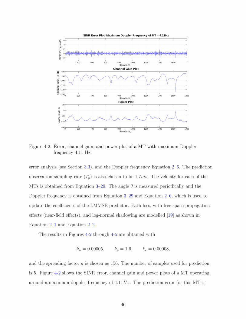
4-2 Error, channel gain, and power plot of a MT with maximum Doppler frequency4.11 Hz. . . . . . . . . . . . . . . . . . . . . . . . . . . . . . . . . . . . . . . . . 46
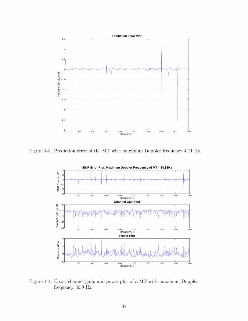
4-3 Prediction error of the MT with maximum Doppler frequency 4.11 Hz. . . . . . 47
4-4 Error, channel gain, and power plot of a MT with maximum Doppler frequency30.9 Hz. . . . . . . . . . . . . . . . . . . . . . . . . . . . . . . . . . . . . . . . . 47
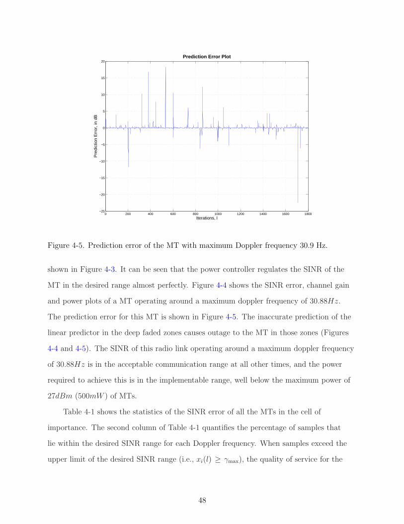
4-5 Prediction error of the MT with maximum Doppler frequency 30.9 Hz. . . . . . 48
4-6 Comparison of high gain and predictive power control algorithms. . . . . . . . . 50
8
Abstract of Thesis Presented to the Graduate Schoolof the University of Florida in Partial Fulfillment of the
Requirements for the Degree of Master of Science
POWER CONTROL OF CDMA-BASED CELLULAR COMMUNICATIONNETWORKS WITH TIME-VARYING STOCHASTIC CHANNEL UNCERTAINTIES
By
Sankrith Subramanian
May 2009
Chair: Warren E. DixonCo-Chair: John M. SheaMajor: Electrical and Computer Engineering
Power control is used to ensure that each link achieves its target signal-to-interference-
plus-noise ratio (SINR) to effect communication in the reverse link (uplink) of a wireless
cellular communication network. In cellular systems using direct-sequence code-division
multiple access (CDMA), the SINR depends inversely on the power assigned to the
other users in the system, creating a nonlinear control problem. Due to the spreading
of bands in CDMA based cellular communication networks, the interference in the
system is mitigated. The nonlinearity now arises by the uncertain random phenomena
across the radio link, causing detrimental effects to the signal power that is desired at
the base station. Mobility of the terminals, along with associated random shadowing
and multi-path fading present in the radio link, results in uncertainty in the channel
parameters. To quantify these effects, a nonlinear MIMO discrete differential equation is
built with the SINR of the radio-link as the state to analyze the behavior of the network.
Controllers are designed based on analysis of this networked system, and power updates
are obtained from the control law. Analysis is also provided to examine how mobility and
the desired SINR regulation range affects the choice of channel update times. Realistic
wireless network mobility models are used for simulation and the power control algorithm
formulated from the control development is verified on this mobility model for acceptable
communication.
9
CHAPTER 1INTRODUCTION
Various transmitter power control methods have been developed to deliver a desired
quality of service (QoS) in wireless networks [1–8]. Early work on power control using a
centralized approach was investigated in [9] and [10]. The concept of Signal-to-Interference
(SIR) balancing was introduced in [9] and [10], where all receivers experience the same SIR
levels. Maximum achievable SIRs were formulated considering the SIR balancing problem
as an eigenvalue problem. A stochastic distributed transmitter power approach was also
investigated in [6–8]. Methods were developed to reduce co-channel interference for a given
channel allocation using transmitter power control in [6] and [8]. In [6], transmitter power
control schemes are developed to reduce the cochannel interferences, the performance
of which is measured by defining Outage probabilities as the probability of having a
too low Signal to Interference (SIR) ratio. An optimum (in the sense that the outage or
interference probability is minimized) eigenvalue based power control scheme is employed
using this approach.
The performance of optimum transmitter power control algorithms is investigated
in [8]. Performance bounds and conditions of stability for all types for transmitter power
control algorithms are found. The system model is developed using N cells with M
independent channel pairs (and hence crosstalk between channels is neglected). The
thermal noise is neglected, as an interference limited system is considered. A link gain
matrix is introduced in [8], each of the components is defined as the link gain from the
base station in cell j to the mobile terminal in cell i, normalized to the link gain in the
desired path, from base station i to mobile terminal i. In [8], a global power control
algorithm is defined as an algorithm that has access to the entire gain matrix in every
instant. An optimum power control algorithm that minimizes the interference probability
is proposed in [8] assuming global power control, and the performance bounds are derived
10
for this algorithm. A Stepwise Removal Algorithm (SRA) is proposed in [8] that minimizes
the computational requirements, suffered by the optimal power control algorithm.
To address the problems associated with measurements of link gains in [8], a
distributed approach was made in [7], where only SIR measurements in those links
actually in use are made. A distributed SIR balancing scheme is developed and a discrete
time power control algorithm (DPCA) is proposed as
P (l + 1) = βZP (l), (1–1)
where P is the power vector, and β is a control gain chosen to avoid increasing powers.
Due to the difficulty in calculating this quantity, a stepwise removal with distributed
balancing scheme is developed in [7]. These algorithms were framed when only path loss
was effecting the channel uncertainty.
A centralized SIR balancing power control scheme was formulated in [11]. Fading and
noise were ignored in this approach. An eigenvalue approach aimed at achieving the same
target SIR for all the radio links is used. An upper limit for the power was imposed to
each user in the constrained power control algorithm of [3], and an optimum power control
for maximizing the minimum SIR is formulated.
A simple distributed autonomous power control algorithm was introduced in [2]
where channel reuse is maximized. Networks where certain power settings exists are
considered and exponential fast convergence to such settings is demonstrated in [2]. Local
measurements were made in [2] to meet the target SINR in each channel. For this purpose,
the distributed control law is manipulated in terms of the power, and SINR for mobile
terminal in a radio link. Making local measurements helps in [2] implies that the SINR for
each radio channel at every sampling instant is measurable, the SINR being a function of
not only a interference in the current cell, but also co-channel interferences from adjacent
cells. Based on the linear analysis of the system, and constraining the eigenvalues, the
power approaches an optimal power vector. The power algorithm formulation for this
11
approach is applicable to both uplink (mobile terminal to base station) and downlink
(base station to mobile terminal) channels.
A framework which integrates power control and base station assignment was
introduced by [12]. A Minimum Transmitted Power (MTP) was formulated for a
CDMA-based system in which the total power is minimized subject to maitaining as
individual target SIR for each mobile. Synchronous (power updates are done at the same
sampling rate for all radio links) and asynchronous (power updates done at different
sampling rates for different radio links) distributed algorithms that find the optimal power
vector and base station assignment is identified.
A generalized framework for uplink iterative power control is provided in [5], where
common properties for interference constraints are identified. The problem of finding the
power control vector for the radio links to achieve acceptable communication is reduced to
satisfying a vector inequality condition stated in [5] as the interference that a user must
overcome to achieve an acceptable connection. Synchronous and asynchronous power
control converge to an optimal power which minimizes the total transmitted power.
Active link protection (ALP) schemes were introduced in [1] and [13], where the QoS
of active links is maintained above a threshold limit to protect the link quality. In [1],
the Foschini-Miljanic power control algorithm is modified for reduced measurements and
emphasis was given on ALP for Distributed Power Control (DPC).
Optimal power control algorithm with outage-probability constraints was developed
in [14], where the network is interference-limited with Rayleigh fading of both the desired
and interference signals. Power control with joint Multiuser Detection (MUD) scheme was
developed in [15] for Rayleigh faded systems with outage constraints.
Recently, a distributed power control scheme was suggested in [16] in the presence
of radio channel uncertainties caused by mobility of the user terminals. These channel
uncertainties include exponential path loss, shadowing, and multi-path fading, which
are modeled as random variables in the SINR measurements. The uncertainty of the
12
multi-path fading effects provided motivation for the results in [16] and [17]. Specifically,
a persistently exciting adaptation scheme is proposed in [16] and [17]. However, in these
works, the fading process is modeled as slowly changing so that the channel gain can be
accurately estimated and practical limitations of transmission power limitations are not
considered.
Of the channel uncertainties, multi-path fading has the most critical effect on the
design of a power-control system because of the time and amplitude scales. Multi-path
fading is caused by reflections in the environment, which cause multiple time-delayed
versions of the transmitted signal to add together at the receiver. The time offsets
cause the signals to add with different phases, and thus multi-path fading can change
significantly over distance scales as short as a fraction of a wavelength. For instance,
for a system using the 900 MHz cellular band, the channel coherence time (the time
for which the channel is essentially invariant) for a mobile terminal traveling at 30
miles/hour is approximately 10 ms. There is a need to quantify the multi-path fading
effects of the channel in the system. In this thesis, efforts are made to understand
the fading phenomena in the radio channel of a CDMA-based cellular communication
network and quantify them to develop power control algorithms. The modeling of cellular
communication networks is based on analysis of the nonlinear networked system and
Lyapunov-based control structures are formulated for such systems in this thesis. An
analytical approach to choosing power update sampling time is used in this thesis where
channel uncertainties (especially Rayleigh fading) are quantified based on estimation of
error between the desired and actual Signal-to-Interference plus Noise Ratio (SINR).
13
CHAPTER 2RADIO-CHANNEL MODELING
In this chapter, the characterictics of the reverse link of the radio channel is
investigated and modeled.
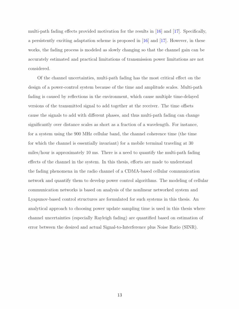
The channel gain of a radio link (see Figure 2-1) is comprised of three components:
Exponential path-loss, Log-normal shadowing, and Multi-path fading. The gain of the
channel is defined [18] as
gii(l) = gd0
(
di(l)
d0
)−κ
100.1δi(l)|Xi(l)|2, (2–1)
where the term |Xi(l)|2 is used to model Rayleigh fading., gd0 is the near-field gain given
by [19]
gd0 =GtGrλ
2
(4π)2 d20L
, df ≤ d0 ≤ di(l), (2–2)
where Gt is the transmitter antenna gain, Gr is the receiver antenna gain, λ is the
wavelength in meters, L is the system-loss factor, d0 is the distance between the
transmitter and receiver antenna, and df = 6m is the Fraunhofer distance. Without
loss of generality, Gt, Gr, and L are all assumed to be 1. Since the power updates are
provided at discrete instances due to bandwidth constraints, the system is analyzed at
discrete instances of time (l ∈ Z). For this reason, the continuous time channel parameters
are analyzed and a suitable channel sampling time is chosen in Chapter 3.
The term(
di(l)d0
)−κ
is used to model the average path loss at distance di(l) from
mobile terminal (MT) i to the base station (BS), where κ is the path-loss exponent, which
typically takes values between two and five. The term 100.1δi(l) is used to model large-scale
log-normal shadowing from buildings, terrain, or foliage, where δi(l) is a Gaussian random
process (see [19]).
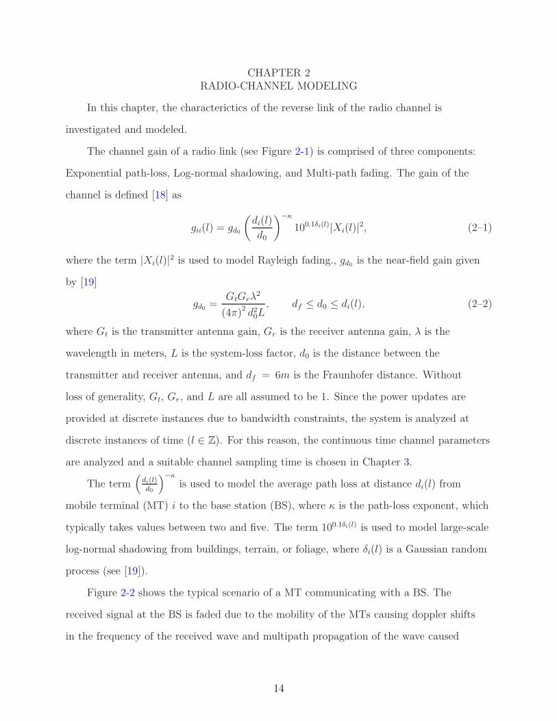
Figure 2-2 shows the typical scenario of a MT communicating with a BS. The
received signal at the BS is faded due to the mobility of the MTs causing doppler shifts
in the frequency of the received wave and multipath propagation of the wave caused
14
Figure 2-1. Reverse link.
Figure 2-2. Fading due to Doppler shift and scattering.
15
by scattering in the presence of surrounding objects. These individual components add
up in a constructive or destructive manner, depending on random phase shifts of these
components of the received signal.
The received fading component of the signal can be represented as [19]
Xi(t) = Gc(t) cos(2πfct) − Gs(t) sin(2πfct) (2–3)
where fc is the carrier frequency, the Gaussian random processes Gc(t) and Gs(t) are
defined as
Gc(t) = E0
N∑
n=1
Cn cos(2πfnt + φn) (2–4)
Gs(t) = E0
N∑
n=1
Cn sin(2πfnt + φn). (2–5)
The processes Gc(t) and Gs(t) are uncorrelated zero-mean Gaussian random variables
for any t with equal varianceE2
0
2, where E0 is the real amplitude of the local average
E-field (assumed constant), Cn is the real random variable representing the amplitude of
individual waves, φn is the phase shift due to reflections of the individual waves and is an
uniform random variable in [0, 2π], N is the number of scattered waves, and fn(t) is the
doppler frequency defined as
fn =v
λcos θ. (2–6)
In Equation 2–6, v(t) is the velocity of motion of the MT and θ(t) is the angle between the
transmitted signal and the direction of motion of the MT.
The envelope of the received signal (E-field) is
|Xi(t)| =√
G2c(t) + G2
s(t), (2–7)
16
0 0.5 1 1.5 2 2.5 3 3.5 4 4.5 50
0.1
0.2
0.3
0.4
0.5
0.6
0.7
Rayleigh Variable, X
f(X
)
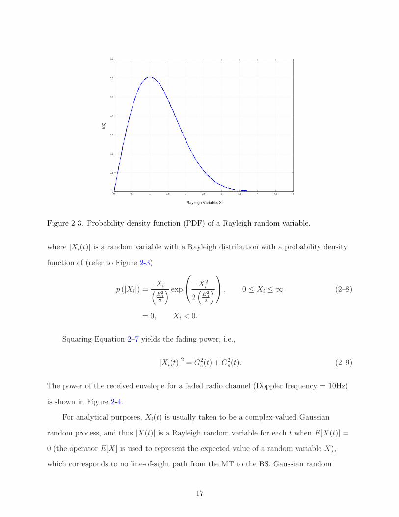
Figure 2-3. Probability density function (PDF) of a Rayleigh random variable.
where |Xi(t)| is a random variable with a Rayleigh distribution with a probability density
function of (refer to Figure 2-3)
p (|Xi|) =Xi(
E20
2
) exp
X2i
2(
E20
2
)
, 0 ≤ Xi ≤ ∞ (2–8)
= 0, Xi < 0.
Squaring Equation 2–7 yields the fading power, i.e.,
|Xi(t)|2 = G2
c(t) + G2s(t). (2–9)
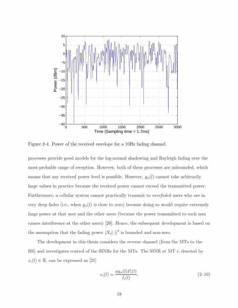
The power of the received envelope for a faded radio channel (Doppler frequency = 10Hz)
is shown in Figure 2-4.
For analytical purposes, Xi(t) is usually taken to be a complex-valued Gaussian
random process, and thus |X(t)| is a Rayleigh random variable for each t when E[X(t)] =
0 (the operator E[X] is used to represent the expected value of a random variable X),
which corresponds to no line-of-sight path from the MT to the BS. Gaussian random
17
0 500 1000 1500 2000 2500 3000−40
−35
−30
−25
−20
−15
−10
−5
0
5
10
Time (Sampling time = 1.7ms)
Pow
er (
dBm
)
Figure 2-4. Power of the received envelope for a 10Hz fading channel.
processes provide good models for the log-normal shadowing and Rayleigh fading over the
most-probable range of reception. However, both of these processes are unbounded, which
means that any received power level is possible. However, gii(l) cannot take arbitrarily
large values in practice because the received power cannot exceed the transmitted power.
Furthermore, a cellular system cannot practically transmit to overfaded users who are in
very deep fades (i.e., when gii(l) is close to zero) because doing so would require extremely
large power at that user and the other users (because the power transmitted to each user
causes interference at the other users) [20]. Hence, the subsequent development is based on
the assumption that the fading power |Xi(·)|2 is bounded and non-zero.
The development in this thesis considers the reverse channel (from the MTs to the
BS) and investigates control of the SINRs for the MTs. The SINR at MT i, denoted by
xi(l) ∈ R, can be expressed as [21]
xi(l) =agii(l)Pi(l)
Ii(l), (2–10)
18
where Pi(l) ∈ R is the power from the MT i to the BS, and gii(l) ∈ R is the channel gain
from the BS to the MT i. In Equation 2–10, Ii(l) ∈ R denotes the interference-plus-noise
power at the BS due to transmissions by other MTs in the cellular network, defined as
Ii(l) =∑
j 6=i
gij(l)Pj(l) + aηi, (2–11)
where gij(l) ∈ R is the channel gain for the link between MT j and the BS that affects
the interference in the radio link between MT i and the BS, Pj(l) ∈ R is the power
transmitted by MT j to the BS, and ηi ∈ R denotes the thermal noise in link i. In a
CDMA based network, each radio link is forced to share the same bandwidth; hence, Ii(·)
is non-zero and bounded. The bandwidth spreading factor, or the processing gain [22] for
the cellular system using CDMA is denoted by a defined as
a =W
R, (2–12)
where W is the transmission bandwidth, in hertz, and R is the data rate in bits/second.
By increasing the bandwidth spreading factor, the interference of the system can be
reduced. Therefore, focus is laid on the effects of fading in the radio channel in this
thesis to develop power controllers for radio links operating in a CDMA based cellular
communication network.
The first difference of the SINR defined in Equation 2–10 can be determined as
∆xi(l) = a (Ii(l) + ∆Ii(l))−1
(
∆gii(l)
Ts
)
Pi(l) + a (Ii(l) + ∆Ii(l))−1 gii(l)
(
∆Pi(l)
Ts
)
− Ii(l) (Ii(l) + ∆Ii(l))−1
a
(
∑
i6=j
(
∆gij(l)Pj(l)
Ts
)
)
gii(l)Pi(l)
+a
(
∑
i6=j
(
gij(l)∆Pj(l)
Ts
)
)
gii(l)Pi(l)
+[
a (Ii(l) + ∆Ii(l))−1
.
(
∆gii(l)
Ts
)(
∆Pi(l)
Ts
)
− a∑
i6=j
(
∆gij(l)∆Pj(l)
T 2s
)
. Ii(l) (Ii(l) + ∆Ii(l))−1 gii(l)Pi(l)
]
(2–13)
19
where Equation 2–10 and Equation 2–11 were used, and Ts is the power update interval.
Neglecting the residual terms in square brackets in Equation 2–13, approximating
(Ii(l) + ∆Ii(l)) ≈ Ii(l), and using Equation 2–10 yields
xi(l + 1) = αi(l, x)xi(l) + ui(l), (2–14)
where αi(l, x) ∈ R is an unknown, time-varying state-dependent quantity, defined as
αi(l, x) = agii(l + 1)g−1ii (l) − a
(
∑
i6=j
(∆gij(l)Pj(l))
)
I−1i (l) − a
(
∑
i6=j
(gij(l)∆Pj(l))
)
I−1i (l)
=⇒ αi(l, x) = aI−1i (l)Pi(l)
[
gii(l + 1)
xi(l)−∑
i6=j
(∆gij(l)Pj(l))
Pi(l)+∑
i6=j
(gij(l)∆Pj(l))
Pi(l)
]
, (2–15)
and ui(l) ∈ R is the control input, defined as
ui(l) =xi(l)
Pi(l)[Pi(l + 1) − Pi(l)] , (2–16)
since
agii(l)
Ii(l)=
xi(l)
Pi(l).
After including measurement noise ξi(l, x), the expression in Equation 2–14 can be
rewritten as
xi(l + 1) = αi(l, x)xi(l) + ui(l) + ξi(l, x). (2–17)
By defining the interference I(l) ∈ Rn×n as a diagonal matrix with entries Ii(l) expressed
in Equation 2–11, g(l) ∈ Rn×n as a diagonal matrix with entries gii(l), and P (l) ∈ R
n, then
the MIMO system can be developed as
x(l + 1) = α(l, x)x(l) + u(l) + ξ(l, x), (2–18)
where α(l, x) = diag (αi(l, x)) ∈ Rn×n denotes the unknown, time-varying state-dependent
diagonal matrix (since αi(l, x) is a function of the state xi(l) as shown in the Equation
2–15) which can be assumed to be upper bounded by a known positive constant from the
preceding discussion on the uncertain channel parameters, x(l) ∈ Rn is the state vector at
20
instant l, u(l) ∈ Rn is the control input vector, x(l + 1) ∈ R
n is the state vector at instant
l + 1, and ξ(l, x) ∈ Rn is the stochastic measurement noise bounded by a known constant.
The measurement noise is assumed to be bounded by a positive constant.
Here, u(l) is expressed in terms of the power update law as
Pi(l + 1) =ui(l)
xi(l)Pi(l) + Pi(l). (2–19)
21
CHAPTER 3ROBUST POWER CONTROL OF CELLULAR COMMUNICATION NETWORKS
WITH TIME-VARYING CHANNEL UNCERTAINTIES
In this chapter, the objective is to design and analyze the performance of a controller
for use in a radio channel operating in a CDMA based cellular communication network
with Rayleigh fading following Clarke’s model [23]. The Rayleigh fading process produces
unbounded changes in the SINRs with non-zero probability, even for arbitrarily short
time scales, but by using the concept of overfaded users [20], the channel gains can be
bounded. Based on this model, a simple proportional controller to minimize the sampled
SINR error is developed in this chapter. Specifically, despite uncertainty in the multi-path
fading effects, a Lyapunov-based analysis is used to develop an ultimate bound for the
sampled SINR error which is a function of the upper bound on the channel uncertainty
divided by a nonlinear damping gain that can be made arbitrarily large up to some upper
value dictated by the power update law. The performance of this controller is evaluated
in this chapter via simulation under realistic power limits and channel changes based on
the standard random-waypoint mobility model. A statistical analysis of the performance
effects of fading between the sampling intervals is considered in this chapter, which is
used to discuss the choice of the control update rate. Additional analysis is provided
to conclude that the expected value of the squared norm of the SINR error converges
to an ultimate bound that is a function of sampling rate. Therefore, the sampling rate
can be adjusted to keep the SINR error within a desired range that allows for signal
decoding. Simulation results are provided for a Random-Waypoint model that illustrates
the performance of the developed controller.
3.1 Control Development
3.1.1 Control Objective
The SINR should remain between two thresholds as
γmin ≤ xi ≤ γmax (3–1)
22
to achieve acceptable communication performance over the link while minimizing
interference to adjacent cells. The control objective for the following development is
to regulate the SINR to a target value for each channel, denoted by γ ∈ Rn, while ensuring
that the SINR remains between the specified lower and upper limits for each channel,
as described in Equation 3–1. To quantify the objective, a regulation error e(l) ∈ Rn is
defined as
e(l) = x(l) − γ. (3–2)
3.1.2 Closed-Loop Error System
The first difference of the regulation error, denoted as ∆e(l) ∈ Rn, is
∆e(l) = e(l + 1) − e(l) = x(l + 1) − x(l) (3–3)
= α(l, x)x(l) + u(l) + ξ(l, x) − x(l).
To facilitate the subsequent analysis, the expression in Equation 3–3 is rewritten as
∆e(l) = χ(l, x) + Ω(l, x) + u(l), (3–4)
where χ(l, x) ∈ Rn denotes an auxiliary term defined as
χ(l, x) =(
α(l, x) − In×1)
e(l), (3–5)
and Ω(l, x) ∈ Rn is defined as
Ω(l, x) =(
α(l, x) − In×1)
γ + ξ(l, x). (3–6)
Motivation for introducing the auxiliary terms in Equation 3–5 and Equation 3–6 is to
collect terms that have a common upper bound. Specifically, upper bounds for χ(l, x) and
Ω(l, x) can be developed as
‖χ(l, x)‖ ≤ c1‖e(l)‖ and ‖Ω(l, x)‖ ≤ c2, (3–7)
23
where c1, c2 ∈ R denote known positive constants. Based on Equation 3–4, Equation 3–7,
and the subsequent stability analysis, a proportional controller is designed as
u(l) , − (c1 + kn + k1) e(l), (3–8)
where c1 is introduced in Equation 3–7, and k1, kn ∈ R denote positive control gains.
Based on Equation 2–19 and Equation 3–8, the power update law is
Pi(l + 1) =− (c1 + kn + k1) ei(l)Pi(l)
(ei(l) + γ)+ Pi(l) (3–9)
under the constraint that 0 < Pi(l) ≤ Pmax, where Pmax is a maximum power level. After
substituting Equation 3–8 into Equation 3–4, the closed-loop error system for e(l) can be
determined as
∆e(l) = χ(l, x) + Ω(l, x) − (c1 + kn + k1) e(l).
3.2 Stability Analysis
Theorem 3-1: The controller in Equation 3–8 and Equation 3–9 ensures that the
SINR regulation error approaches an ultimate bound ε(kn, l0) ∈ R in the sense that
‖e(l)‖ → ε(kn, l0) as l → ∞. (3–10)
Proof: Let V (e, l) : D × [0,∞) → R be a positive definite function defined as
V (e, l) =1
2eT (l)e(l). (3–11)
After taking the first difference of Equation 3–11, substituting Equation 3–4 into the
resulting expression, and then cancelling common terms, the following expression can be
obtained:
∆V = eT (l)χ(l, x) + eT (l)Ω(l, x) − (c1 + kn + k1) eT (l)e(l). (3–12)
24
By using Equation 3–7, the expression in Equation 3–12 can be upper bounded as
∆V ≤ c1‖e(l)‖2 + c2‖e(l)‖ − (c1 + kn + k1)‖e(l)‖
2
≤ c2‖e(l)‖ − kn‖e(l)‖2 − k1‖e(l)‖
2. (3–13)
Completing the squares on the first two terms in Equation 3–13 yields the following upper
bound
∆V ≤ −k1V (e, l) +c22
4kn. (3–14)
Lemma 13.1 of [24] can now be invoked to conclude that
V (e, l) ≤ blV (e(l0), l0) +
(
1 − bl
k1
)
c22
4kn, (3–15)
where
b = 1 − k1,
where 0 < k1 ≤ 1. Based on Equation 3–15, an upper bound for e(l) can be developed as
‖e(l)‖2 ≤ bl‖e(l0)‖2 +
(
1 − bl
k1
)
c22
4kn. (3–16)
The ultimate bound in Equation 3–16 asymptotically converges as
liml→∞
‖e(l)‖2 =c22
4k1kn. (3–17)
From Equation 3–17, the ultimate bound can be decreased by increasing kn; however, the
magnitude of kn is restricted by Equation 3–9 and the constraint that 0 < Pi(l) ≤ Pmax.
3.3 Estimation of Error at Unsampled Instances
The developed controller operates at discrete times using a predefined sampling rate.
The stability analysis in Section 3.2 only proves that the controller can achieve arbitrarily
low error at the sampling times. In this section, an approximate analysis of the error is
provided between the sampling times, and the mean-squared error is shown to be bounded
by a constant that depends on the time between samples.
25
Consider the performance for large t, such that the error magnitude satisfies |e(l)| =
|x(l) − γ| < ε. Let Ts denote the time between samples. Then the error for the signal from
MT i at time t, where lTs < t < (l + 1)Ts is
ei(t) = xi(t) − γ =gii(t)Pi(t)
Iai (t)
− γ. (3–18)
Letting ∆gii(t) = gii(t) − gii(lTs) and using Equation 2–11, the error can be written as
ei(t) =a[gii(l) + ∆gii(t)]Pi(t)
∑
j 6=i
[gij(l) + ∆gij(t)]Pj(l) + aηi(t)− γ
=agii(l)Pi(t) + a∆gii(t)Pi(t)
∑
j 6=i
gij(l)Pj(l) +∑
j 6=i
∆gij(t)Pj(l) + aηi(t)− γ. (3–19)
To facilitate the analysis, under the assumption of a large number of mobile stations
operating in the current cell, the weak law of large numbers can be invoked to approximate
the second term in the denominator as
∑
j 6=i
∆gij(t)Pj(l) ≈∑
j 6=i
E[∆gij(t)] = 0. (3–20)
Thus, the magnitude of the error can be approximated as
|ei(t)| ≈
∣
∣
∣
∣
∣
∣
∣
agii(l)Pi(t) + a∆gii(t)Pi(t)∑
j 6=i
gij(l)Pj(l) + aηi(t)− γ
∣
∣
∣
∣
∣
∣
∣
,
and upper bounded by
|ei(t)| <
∣
∣
∣
∣
∣
∣
∣
a∆gii(t)Pi(t)∑
j 6=i
gij(l)Pj(l) + aηi(t)
∣
∣
∣
∣
∣
∣
∣
+ εCT . (3–21)
Noting that E[∆gii(t)] = 0, the mean-squared error at time t is bounded by
E[e2i (t)] <
a2E[∆g2ii(t)]P
2i (t)
[
∑
j 6=i
gij(l)Pj(l) + aηi(t)
]2 + ε2CT , (3–22)
26
where the expectation E[∆g2ii(t)] is with respect to the random change in the fading
∆gii(t).
Let Rg(τ) be the autocorrelation function of the channel gain process. The expected
value in Equation 3–22 can be written as
E[∆g2ii(t)] = E
[g(t) − g(lTs)]2
= E[g2(t)] − 2E[g(t)g(lT s)] + E[g2(lT s)]
= 2Rg(0) − 2RG(τ), (3–23)
where τ = t − lT s. In most systems, the sampling time will be fast enough that the
exponential path loss and shadowing can be modeled as constant between sampling times,
and thus the effects of multi-path fading is only considered. The autocorrelation function
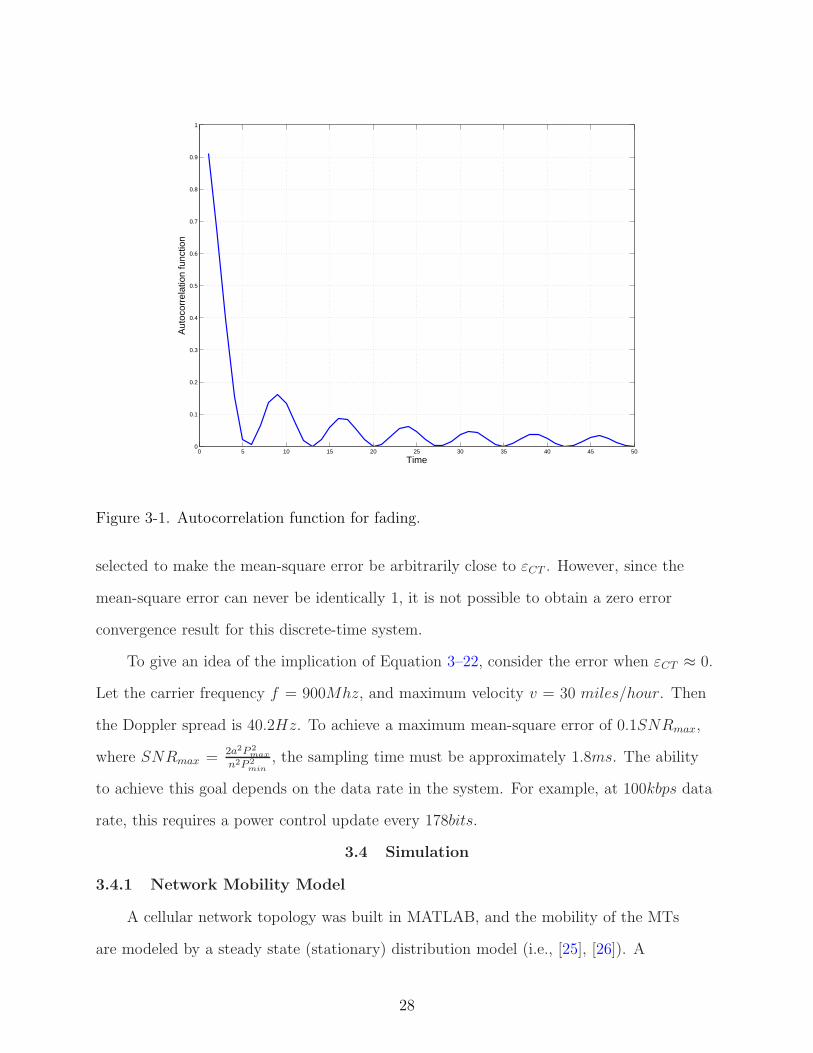
for the power in a Rayleigh fading process (refer to Figure 3-1) is given by [23]
Rg(τ) = J20 (2πfnτ), (3–24)
where J0 is the zeroth-order Bessel function of the first kind, and fn is the Doppler spread.
The Doppler spread is given by fv/c, where f is the carrier frequency, v is the mobile
velocity, and c is the speed of light.
Then, the mean-squared error is bounded by
E[e2i (t)] <
2a2 [1 − J20 (2πfnτ)] P 2
i (t)[
∑
j 6=i
gij(l)Pj(l) + ηi(t)
]2 + ε2CT
< 2a2[
1 − J20 (2πfnTs)
] P 2max
n2P 2min
+ ε2CT , (3–25)
where the weak law of large numbers is applied to the denominator with E[g2ij(l)] = 1.
Here, Pmax and Pmin are, respectively, the maximum and minimum transmit powers
allocated to a non-overfaded user. By taking into account the maximum power ratio
Pmax/Pmin, number of users n, spreading gain a, and maximum MT velocity, Ts can be
27
0 5 10 15 20 25 30 35 40 45 500
0.1
0.2
0.3
0.4
0.5
0.6
0.7
0.8
0.9
1
Aut
ocor
rela
tion
func
tion
Time
Figure 3-1. Autocorrelation function for fading.
selected to make the mean-square error be arbitrarily close to εCT . However, since the
mean-square error can never be identically 1, it is not possible to obtain a zero error
convergence result for this discrete-time system.
To give an idea of the implication of Equation 3–22, consider the error when εCT ≈ 0.
Let the carrier frequency f = 900Mhz, and maximum velocity v = 30 miles/hour. Then
the Doppler spread is 40.2Hz. To achieve a maximum mean-square error of 0.1SNRmax,
where SNRmax = 2a2P 2max
n2P 2min
, the sampling time must be approximately 1.8ms. The ability
to achieve this goal depends on the data rate in the system. For example, at 100kbps data
rate, this requires a power control update every 178bits.
3.4 Simulation
3.4.1 Network Mobility Model
A cellular network topology was built in MATLAB, and the mobility of the MTs
are modeled by a steady state (stationary) distribution model (i.e., [25], [26]). A
28
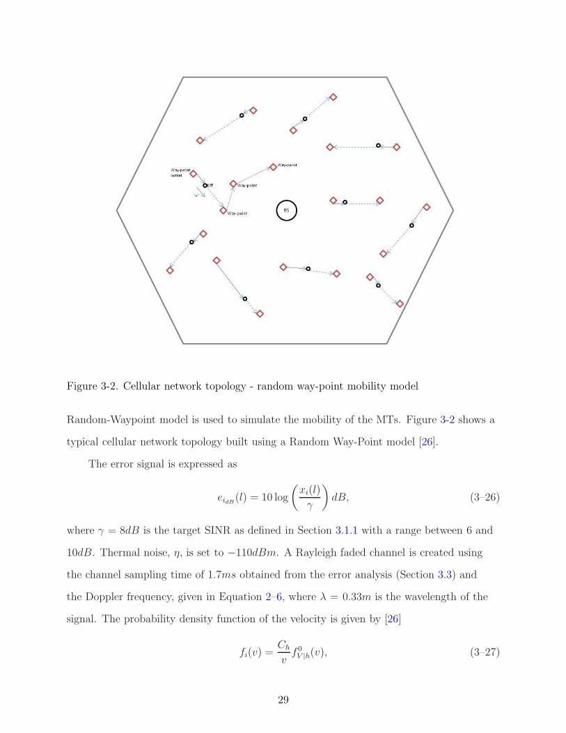
Figure 3-2. Cellular network topology - random way-point mobility model
Random-Waypoint model is used to simulate the mobility of the MTs. Figure 3-2 shows a
typical cellular network topology built using a Random Way-Point model [26].
The error signal is expressed as
eidB(l) = 10 log
(
xi(l)
γ
)
dB, (3–26)
where γ = 8dB is the target SINR as defined in Section 3.1.1 with a range between 6 and
10dB. Thermal noise, η, is set to −110dBm. A Rayleigh faded channel is created using
the channel sampling time of 1.7ms obtained from the error analysis (Section 3.3) and
the Doppler frequency, given in Equation 2–6, where λ = 0.33m is the wavelength of the
signal. The probability density function of the velocity is given by [26]
fi(v) =Ch
vf 0
V |h(v), (3–27)
29
0 500 1000 1500 2000 2500 3000−30
−25
−20
−15
−10
−5
0
5
10
15
20
Iterations, l
Err
or, i
n dB
Doppler freq.=1.98HzDoppler freq.=4.71HzDoppler freq.=2.49HzDoppler freq.=9.86HzDoppler freq.=3.25HzDoppler freq.=6.35Hz
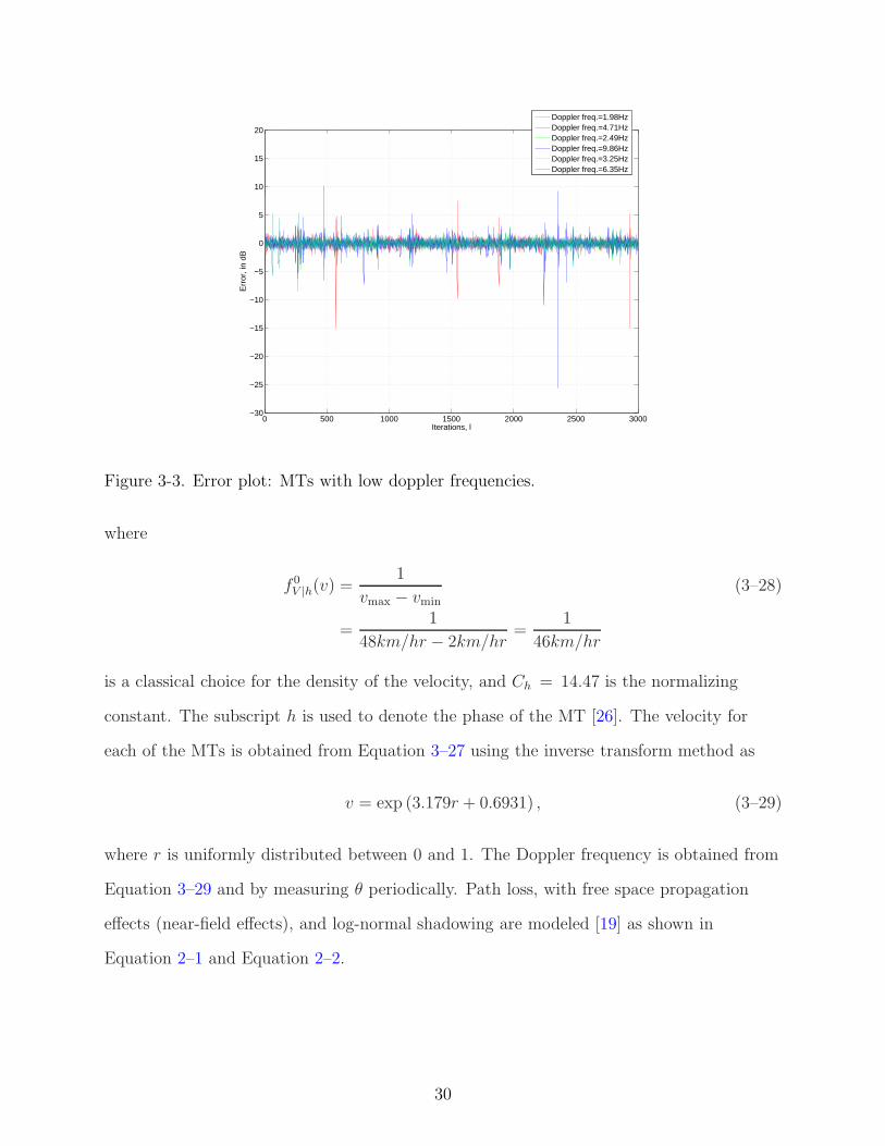
Figure 3-3. Error plot: MTs with low doppler frequencies.
where
f 0V |h(v) =
1
vmax − vmin(3–28)
=1
48km/hr − 2km/hr=
1
46km/hr
is a classical choice for the density of the velocity, and Ch = 14.47 is the normalizing
constant. The subscript h is used to denote the phase of the MT [26]. The velocity for
each of the MTs is obtained from Equation 3–27 using the inverse transform method as
v = exp (3.179r + 0.6931) , (3–29)
where r is uniformly distributed between 0 and 1. The Doppler frequency is obtained from
Equation 3–29 and by measuring θ periodically. Path loss, with free space propagation
effects (near-field effects), and log-normal shadowing are modeled [19] as shown in
Equation 2–1 and Equation 2–2.
30
0 500 1000 1500 2000 2500 3000−25
−20
−15
−10
−5
0
5
10
15
20
25
Iterations, l
Err
or
(dB
)
Doppler Freq. = 34.14HzDoppler Freq. = 18.36HzDoppler Freq. = 18.28HzDoppler Freq. = 10.84Hz
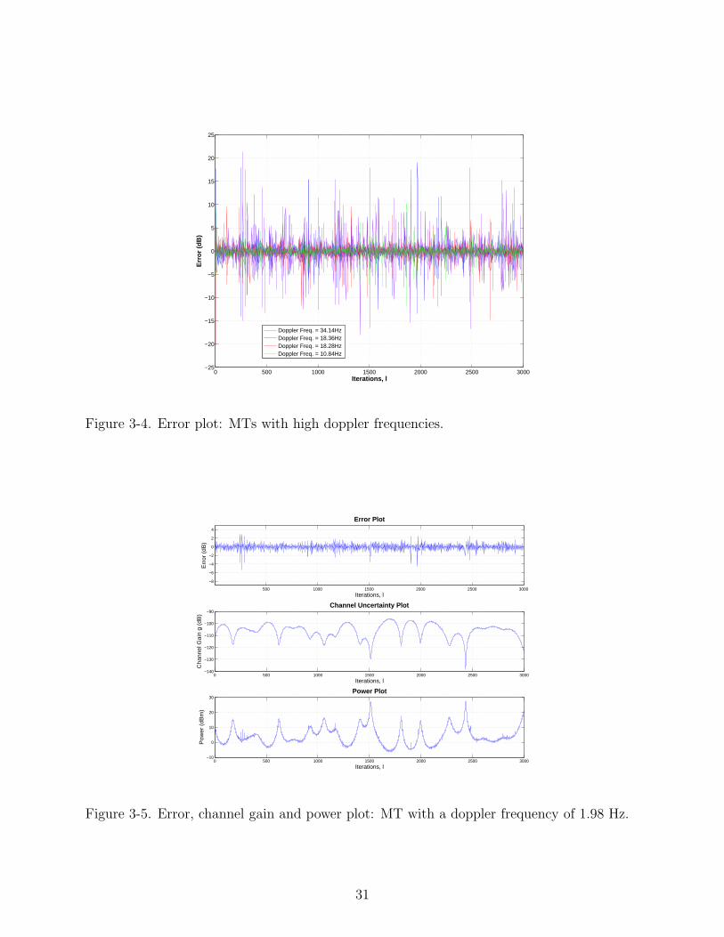
Figure 3-4. Error plot: MTs with high doppler frequencies.
500 1000 1500 2000 2500 3000
−8
−6
−4
−2
0
2
4
Iterations, l
Err
or (
dB)
Error Plot
0 500 1000 1500 2000 2500 3000−140
−130
−120
−110
−100
−90
Iterations, l
Cha
nnel
Gai
n g
(dB
)
Channel Uncertainty Plot
0 500 1000 1500 2000 2500 3000−10
0
10
20
30
Iterations, l
Pow
er (
dBm
)
Power Plot
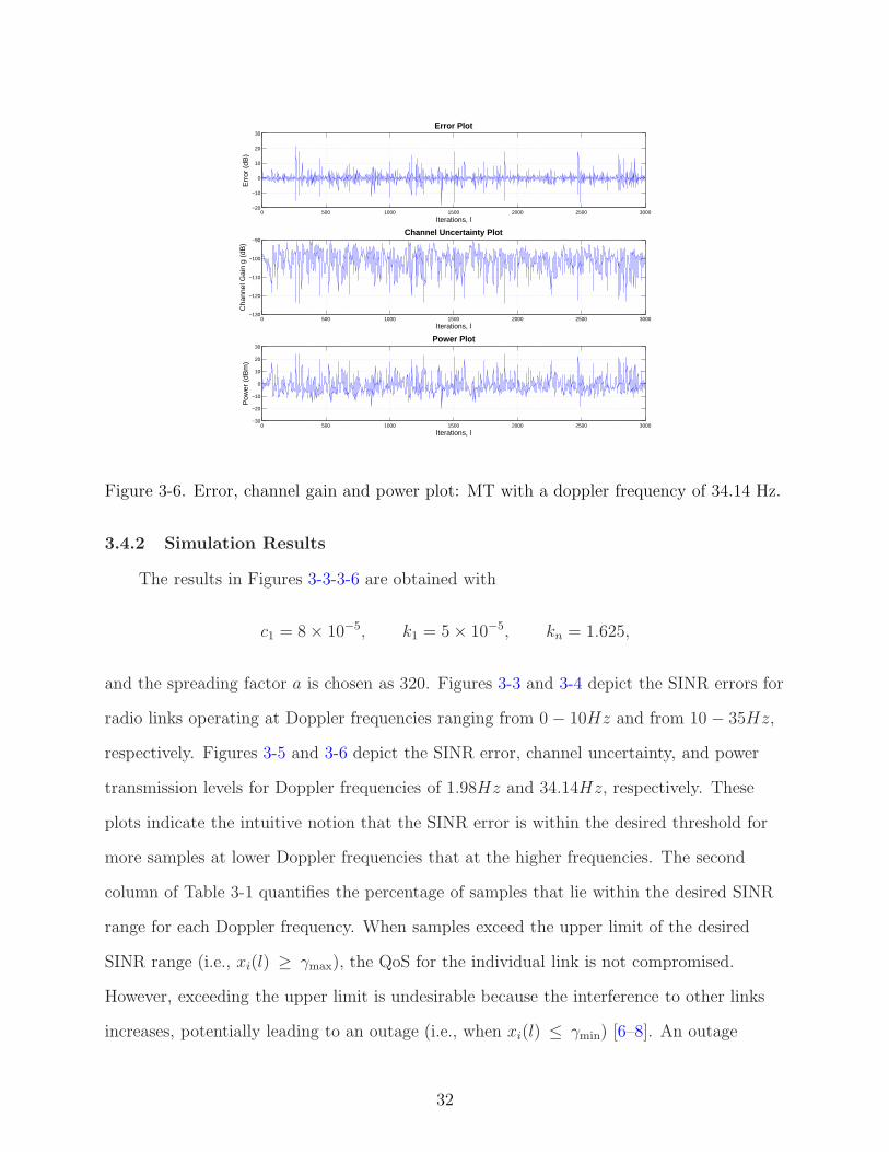
Figure 3-5. Error, channel gain and power plot: MT with a doppler frequency of 1.98 Hz.
31
0 500 1000 1500 2000 2500 3000−20
−10
0
10
20
30
Iterations, l
Err
or (
dB)
Error Plot
0 500 1000 1500 2000 2500 3000−130
−120
−110
−100
−90
Iterations, l
Cha
nnel
Gai
n g
(dB
)Channel Uncertainty Plot
0 500 1000 1500 2000 2500 3000−30
−20
−10
0
10
20
30
Iterations, l
Pow
er (
dBm
)
Power Plot
Figure 3-6. Error, channel gain and power plot: MT with a doppler frequency of 34.14 Hz.
3.4.2 Simulation Results
The results in Figures 3-3-3-6 are obtained with
c1 = 8 × 10⁻⁵, k1 = 5 × 10⁻⁵, kn = 1.625,
and the spreading factor a is chosen as 320. Figures 3-3 and 3-4 depict the SINR errors for
radio links operating at Doppler frequencies ranging from 0 − 10Hz and from 10 − 35Hz,
respectively. Figures 3-5 and 3-6 depict the SINR error, channel uncertainty, and power
transmission levels for Doppler frequencies of 1.98Hz and 34.14Hz, respectively. These
plots indicate the intuitive notion that the SINR error is within the desired threshold for
more samples at lower Doppler frequencies that at the higher frequencies. The second
column of Table 3-1 quantifies the percentage of samples that lie within the desired SINR
range for each Doppler frequency. When samples exceed the upper limit of the desired
SINR range (i.e., xi(l) ≥ γmax), the QoS for the individual link is not compromised.
However, exceeding the upper limit is undesirable because the interference to other links
increases, potentially leading to an outage (i.e., when xi(l) ≤ γmin) [6–8]. An outage
32
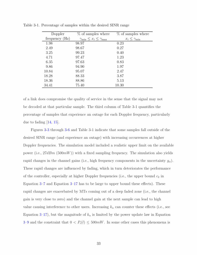
Table 3-1. Percentage of samples within the desired SINR range
Dopplerfrequency (Hz)
% of samples whereγmin ≤ xi ≤ γmax
% of samples wherexi ≤ γmin
1.98 98.97 0.232.49 98.67 0.273.25 99.23 0.404.71 97.47 1.236.35 97.63 0.839.86 94.90 1.97
10.84 95.07 2.4718.28 88.33 3.8718.36 88.86 5.1334.41 75.40 10.30
of a link does compromise the quality of service in the sense that the signal may not
be decoded at that particular sample. The third column of Table 3-1 quantifies the
percentage of samples that experience an outage for each Doppler frequency, particularly
due to fading [14, 15].
Figures 3-3 through 3-6 and Table 3-1 indicate that some samples fall outside of the
desired SINR range (and experience an outage) with increasing occurrences at higher
Doppler frequencies. The simulation model included a realistic upper limit on the available
power (i.e., 27dBm (500mW )) with a fixed sampling frequency. The simulation also yields
rapid changes in the channel gains (i.e., high frequency components in the uncertainty gii).
These rapid changes are influenced by fading, which in turn deteriorates the performance
of the controller, especially at higher Doppler frequencies (i.e., the upper bound c2 in
Equation 3–7 and Equation 3–17 has to be large to upper bound these effects). These
rapid changes are exacerbated by MTs coming out of a deep faded zone (i.e., the channel
gain is very close to zero) and the channel gain at the next sample can lead to high
value causing interference to other users. Increasing kn can counter these effects (i.e., see
Equation 3–17), but the magnitude of kn is limited by the power update law in Equation
3–9 and the constraint that 0 < Pi(l) ≤ 500mW . In some other cases this phenomena is
33

coupled with over-fading, when the power of some MTs reach an upper saturation limit
and the controller can no longer increase the power to compensate for the fading.
34
CHAPTER 4PREDICTION-BASED POWER CONTROL OF DISTRIBUTED CELLULAR
COMMUNICATION NETWORKS WITH TIME-VARYING CHANNELUNCERTAINTIES
Fast changing radio channels in a CDMA based cellular network have detrimental
effects on the control efforts required to regulate the SINR to the desired level, especially
for channels with high doppler frequency MTs. The motivation behind introducing a
prediction-based power control algorithm is to meet the problems associated with rapid
changes in the channel gain (by orders of magnitude between power update intervals)
influenced by fading and exacerbated by the MTs coming out of the ’deep faded’ zone.
For a fast fading channel, a reliable prediction of the channel coefficient is required for
accurate control design. For this purpose, a linear prediction filter is used in this chapter
to estimate the channel fading parameter and this information is fed to the controller.
A controller is developed in this chapter that uses local SINR measurements from the
current and neighboring cells ([2], [1]) to maintain the SINRs of all the MTs present in
the acceptable communication range. A Lyapunov based analysis is provided to explain
the bound which the SINR error reaches, the size of which can be reduced by choosing
appropriate control gains. The power control algorithm is simulated on a cellular network
with distributed cells and the results indicate that the controller regulates the SINRs of all
the MTs with low outage probability.
Due to the fast fading channel that a power controller has to encounter before
ensuring acceptable communication between the MTs and the BS, prediction of the fading
power would provide the controller with useful channel information. Earlier research
conducted by Hallen on fading prediction focused on long range prediction [27–31] based
on the fact that the amplitude, frequency and phase of each multi-path component vary
much slower than the actual fading coefficient Xi(·). In [28], fading channel prediction
is combined with transmitter signal optimization to mitigate the effects of deep fades.
Physical channel modeling, with adaptive prediction was presented in [29]. Consequently,
35
focus was laid on performance analysis of long range prediction, transmitter diversity and
adaptive long range prediction of fast fading channel coefficients [32].
In this chapter, the basic concepts on the radio channel characteristics as discussed
above is analyzed and power of the fading coefficient is predicted, which is used in the
subsequent control design. More specifically, for accurate prediction, more recent samples
are used to estimate the fading coefficient at the next instance, unlike the long range
fading prediction schemes where the goal is to predict the pattern of the fading envelope.
For this purpose, a linear Minimum Mean Square Error (MMSE) predictor is used to
obtain a reliable prediction of the fading coefficient at the next instance. Lyapunov based
analysis is performed to provide an ultimate bound on the SINR error, the size of which
can be reduced by choosing appropriate control gains. In addition, variations in other
components of the radio channel such as path loss and log-normal shadowing are also
accounted for using this analysis tool. Simulation results are provided for analysis and
verification of results, and motivation is provided for future work.
4.1 Network Model
The SINR x(l) ,
[
x1(l) x2(l) . . xn(l)
]T
∈ Rn is defined (in dB) for each radio
link i = 1, 2, ...n as
xi(l) = 10 log
(
agii(l)Pi(l)
Ii(l)
)
(4–1)
where the function log(·) denotes the base 10 logarithm. The quantities inside the log(·)
function of Equation 4–1 is defined in Chapter 3.
Understanding how the SINR changes is beneficial for the development and analysis
of the subsequent power control law. Taking the first difference of Equation 4–1 yields
∆xi(l)
Ts=
xi(l + 1) − xi(l)
Ts
=[10 log(gii(l + 1)) − 10 log(gii(l))]
Ts
+ui(l)
Ts
−[10 log(Ii(l + 1)) − 10 log(Ii(l))]
Ts, (4–2)
36
where Ts is the power update interval, and u(l) ,
[
u1(l) u2(l) . . un(l)
]T
∈ Rn
denotes an auxiliary control signal defined ∀i = 1, 2, ...., n as
ui(l) = 10 [log(Pi(l + 1)) − log(Pi(l))] , (4–3)
which is used to determine the power update law. The reason for defining the state as in
Equation 4–1 is to obtain the controller as Equation 4–3 that would yield a power update
that is more sensitive in operation than the power update Equation 3–9 used in Chapter 3.
After including measurement noise ξ(l, x) ,
[
ξ1(l, x1) ξ2(l, x2) . . ξn(l, xn)
]T
∈
Rn, the SINR at the next update interval x(l+1) ,
[
x1(l + 1) x2(l + 1) . . xn(l + 1)
]T
∈
Rn can be expressed as
x(l + 1) = f1 (x(l)) + f2 (x(l)) + x(l) + u(l) + ξ(l, x), (4–4)
where the channel gain functional f1 (x(l)) ∈ Rn is defined ∀i = 1, 2, ...., n as
f1 (xi(l)) = 10 log
(
gii(l + 1)
gii(l)
)
, (4–5)
and the interference functional f2 (x(l)) ∈ Rn is defined ∀i = 1, 2, ...., n as
f2 (xi(l)) = 10 log
(
Ii(l)
Ii(l + 1)
)
. (4–6)
4.2 Linear Prediction of Fading Coefficient
The development of a power controller for radio links in a CDMA network is
challanging due to rapid, large scale changes in the coefficients of the nonlinear SINR
dynamics. A further challange is that the power capacity at each MT is constrained as
0 < Pi(l) ≤ Pmax,
where Pmax ∈ R is a maximum power level. As indicated in the simulation results in our
previous effort [33], this dual problem leads to signal outages, especially when the MT
37
enters a deep faded zone. Motivated to address these issues, the current result estimates
(or predicts) |Xi(l + 1)|2 and feeds this information to the controller to account for such
fast changing channels and power limitations.
The prediction of |Xi(l + 1)|2 can be defined as a Optimum Mean Square Error
(MSE) problem (see Appendix A), i.e.,
ε2min = min
Xi
E
[
(
|Xi(l + 1)|2 − Xi(l))2]
given |Xi(l)|2 , |Xi(l − 1)|2 , .., |Xi(l − (n1 − 1))|2 ,
where Xi(l) is the estimate of |Xi(l + 1)|2 that reduces the MSE. The optimum estimator
is equal to the conditional mean [34]
E[
|Xi(l + 1)|2 | |Xi(l)|2 , ....., |Xi(l − (n1 − 1))|2
]
,
which is read as the expected value of |Xi(l + 1)|2 given |Xi(l)|2,....., |Xi(l − (n1 − 1))|2.
Obtaining conditional estimate for nongaussian random processes (i.e., |Xi(l + 1)|2)
is difficult; nonlinear estimates might be optimum for such cases and it requires higher
order moments to obtain such nonlinear estimates. For these reasons, a linear estimator is
chosen for predicting the fading variable |Xi(l + 1)|2.
The Linear MMSE for a non-gaussian random variable |Xi(·)|2 can be obtained
from [34] as
Xi(l) =l∑
m=l−(n1−1)
β(m)i
|Xi(m)|2 − µ|Xi|2
+ µ|Xi|2
=
l∑
m=l−(n1−1)
β(m)i
|Xi(m)|2
+µ|Xi|2
(
1 −l∑
m=l−n1
β(m)i
)
; fn 6= 0
|Xi(l)|2 ; fn = 0
(4–7)
where µ|Xi|2 is the mean of the random process |Xi(·)|
2 for all l, fn is the doppler
frequency of the MT defined in Equation 2–6 at instance (lTp + 1) − (lTp). The linear
38
estimate Xi(l) can take non-zero values if the prediction observation sampling rate (Tp)
can be chosen appropriately. Based on [27], the sampling rate is chosen such that it is
atleast the Nyquist rate, i.e., twice the maximum doppler frequency of the MT.
The β(l−1)m ’s satisfy the orthogonality condition [see Appendix B]. Defining βi ,
[
β(l−(n1−1))i β
(l−(n1−2))i ..... β
(l)i
]T
and using the orthogonality condition yields
βTi =
E[
|Xi(l + 1)|2 |Xi(l − (n1 − 1))|2]
E[
|Xi(l + 1)|2 |Xi(l − (n1 − 2))|2]
.
E[
|Xi(l + 1)|2 |Xi(l)|2]
T
Z−1, (4–8)
where Z ∈ Rn1×n1 is defined ∀j, k = 1, 2, ...., n1 as
Zjk = E[
|Xi(l − (n1 − j))|2 |Xi(l − (n1 − k))|2]
.
The autocovariance function for |Xi()|2 is given by [23], [35]
R|Xi|2(lTp) = E
[
|Xi(l)|2 |Xi (l + (lTp))|
2]
≈ J20 (2πfn (lTp)) , (4–9)
(refer Figure 3-1) where J0 is the zeroth-order Bessel function of the first kind. Therefore,
from Equation 4–8,
βTi =
J20 (2πfn (Tpn1))
J20 (2πfn (Tp (n1 − 1)))
.
J20 (2πfnTp)
T
Z−1, fn 6= 0. (4–10)
where the components of Z are defined ∀j, k = 1, 2, ...., n1 as
Zjk = Zkj =
J20 (2πfnTp |j − k|) ; j 6= k
σ|Xi|2 ; j = k
, fn 6= 0. (4–11)
39
By orthogonality, we have the LMMSE [34] as
ε2min = E
[
(
|Xi(l + 1)|2)2]
−l∑
m=l−(n1−1)
βmi E
[
|Xi (m)|2 |Xi (l + 1)|2]
.
Claim 4-1: The Linear predictor in Equation 4–7 is bounded based on the following
facts. The power of the faded envelope |Xi(·)|2 at the receiver is bounded since in a radio
link, the received power cannot be greater than the transmitted power (refer to Chapter
2 and Section 4.1). Therefore, the mean µ|Xi|2 and the variance σ|Xi|
2 are bounded. The
coefficients of βi in Equation 4–10 are bounded if the covariance matrix in Equation 4–11
is invertible. A prediction observation sampling rate (Tp) equal to or lower [31] than the
power update rate (Ts) is chosen (such that it is atleast the Nyquist rate [27]) and the
effect of additive noise is incorporated in Z [27], so that the inverse of Z can be computed.
Linear prediction of the fading process requires measurement of the |X1(·)|2 at the
current and previous instances; the performance of the predictor can be improved by
increasing the number of measurements n1 used to predict the fading process at instance
l + 1. Practically, as more measurements are used, the performance of the predictor
does not improve but degrades due to computational problems associated with inverting
the matrix Z. Note that the fading power of individual MTs at instance l used in the
predictor is also used in the controller in the χX(l) term.
4.3 Control Development
4.3.1 Control Objective
The network quality of service can be quantified by the ability of the SINR to remain
within a specified operating range with upper and lowers limits, γmin, γmax ∈ Rn for each
link defined ∀i = 1, 2, ...., n as
γmin ≤ xi(l) ≤ γmax. (4–12)
Keeping the SINR above the minimum threshold eliminates signal dropout, whereas
remaining below the upper threshold minimizes interference to adjacent cells. As in
Chapter 3, the control objective in this chapter is to regulate the SINR to a target value
40
for each channel, denoted by γ ∈ Rn, while ensuring that the SINR remains between the
specified lower and upper limits for each channel. To quantify this objective, a regulation
error is defined as e(l) ,
[
e1(l) e2(l) . . en(l)
]T
∈ Rn where
ei(l) = xi(l) − γ, ∀i = 1, 2, ...., n. (4–13)
4.3.2 Closed Loop Error System
By taking the first difference of Equation 4–13, and using Equation 2–1, Equation
4–4, and Equation 4–5, the open-loop error dynamics for each link can be determined as
∆ei(l) = 10 log
gd0
(
di(l + 1)
d0
)−κ
100.1δi(l+1) |Xi(l + 1)|2
− 10 log
gd0
(
di(l)
d0
)−κ
100.1δi(l) |Xi(l)|2
+ f2 (xi(l)) + ξi(l, x) + ui(l).
After using properties of the log(·) function, the open-loop error dynamics can be
simplified as
∆e(l) = 10χd(l, l + 1) + χδ(l, l + 1) + 10χX (l + 1)
− 10χX(l) + f2 (x(l)) + ξ(l, x) + u(l), (4–14)
where the auxiliary functions χd(l, l + 1), χδ(l, l + 1), χX (·) ∈ Rn are defined ∀i = 1, 2, ...., n
as
χd(l, l + 1) =
[
κ log
(
d1(l)
d1(l + 1)
)
κ log
(
d2(l)
d2(l + 1)
)
... κ log
(
dn(l)
dn(l + 1)
)]T
, (4–15)
χδ(l, l + 1) = [δ1 (l + 1) − δ1(l) δ2 (l + 1) − δ2(l) ... δn (l + 1) − δn(l)]T , (4–16)
and
χχ(·) =[
log |X1(·)|2 log |X2(·)|
2 ... log |Xn(·)|2]T
. (4–17)
Based on the model development in Chapter 2 (i.e., di(·) and Ii(·) are non-zero and
bounded), the norm of χd(l, l + 1) and f2 (x(l)) can be upper bounded by some positive
41
scalars as
‖χd(l, l + 1)‖ ≤ c1, (4–18)
and
‖f2 (x(l))‖ ≤ c2. (4–19)
Moroever, since δ(·) is a zero-mean gaussian distributed variable (in dB) with a bounded
standard deviation [19], then the norm of χδ(l, l + 1) can be upper bounded by some
positive scalar as
‖χδ(l, l + 1)‖ ≤ c3, (4–20)
and the measurement noise is assumed to be bounded, i.e.,
‖ξ(l, x)‖ ≤ c4. (4–21)
Based on Equation 4–14 and the subsequent stability analysis, the auxiliary power
controller u(l) is designed as
u(l) = − (kn + kp + ke) e(l) − 10Log(∣
∣
∣X(l)
∣
∣
∣
)
+ 10χX(l), (4–22)
where the notation Log(∣
∣
∣X(l)
∣
∣
∣
)
is defined ∀i = 1, 2, ...., n as
Log(∣
∣
∣X(l)
∣
∣
∣
)
=[
log(∣
∣
∣X1(l)
∣
∣
∣
)
log(∣
∣
∣X2(l)
∣
∣
∣
)
... log(∣
∣
∣Xn(l)
∣
∣
∣
)]T
, (4–23)
and∣
∣
∣Xi(·)
∣
∣
∣6= 0, (4–24)
where the components of Log(∣
∣
∣X(l)
∣
∣
∣
)
are obtained from Equation 4–7, and the prediction
sampling rate is chosen to be at least the Nyquist rate for Equation 4–24 to hold. From
Equation 4–3, Equation 4–17, Equation 4–22, and Equation 4–23, the power update law
for each radio channel is obtained as
Pi(l + 1) = 10Ωi, ∀i = 1, 2, ...., n, (4–25)
42
where
Ωi =− (kn + kp + ke) ei(l)
10− log
(∣
∣
∣Xi(l)
∣
∣
∣
)
+ log |Xi(l)|2 + log(Pi(l)). (4–26)
4.4 Stability Analysis
Theorem 4-1: The controller in Equation 4–22 and Equation 4–25 ensures that
all closed loop signals are bounded, and that the SINR regulation error approaches an
ultimate bound ε(kn, kp, l0) ∈ R in the sense that
‖e(l)‖ → ε(kn, kp, l0) as l → ∞ (4–27)
provided ke in Equation 4–22 is selected as
0 < ke ≤ 1. (4–28)
Proof: Let V (e, l) : D × [0,∞) → R be a positive definite function defined as
V (e, l) =1
2eT (l)e(l). (4–29)
Taking the first difference of Equation 4–29, and substituting for Equation 4–14 yields
∆V = eT (l) [10χd(l, l + 1) + χδ(l, l + 1) + 10χX (l + 1)
−10χX(l) + f2 (x(l)) + ξ(l, x) + u(l)] . (4–30)
Using Equations 4–18-4–21, and substituting Equation 4–22 into Equation 4–30 yields
∆V ≤ −ke ‖e(l)‖2 + 10 ‖e(l)‖
(∥
∥
∥χX (l + 1) − Log
(∣
∣
∣X(l)
∣
∣
∣
)∥
∥
∥
)
− kp ‖e(l)‖2
+ (10c1 + c2 + c3 + c4) ‖e(l)‖ − kn ‖e(l)‖2 . (4–31)
By completing the squares for the second and third lines, the inequality in Equation 4–31
can be further upper bounded as
∆V ≤ −ke ‖e(l)‖2 +
25(∥
∥
∥χX (l + 1) − Log
(∣
∣
∣X(l)
∣
∣
∣
)∥
∥
∥
)2
kp+
(10c1 + c2 + c3 + c4)2
4kn.
43
After using Equation 4–29, the following inequality can be developed
∆V ≤ −keV +25(∥
∥
∥χX (l + 1) − Log
(∣
∣
∣X(l)
∣
∣
∣
)∥
∥
∥
)2
kp+
(10c1 + c2 + c3 + c4)2
4kn. (4–32)
Provided the sufficient condition in Equation 4–28 is satisfied, Lemma 13.1 of [24] can be
invoked to conclude that
V (e, l) ≤ (1 − ke)l V (e(l0), l0) +
(
1 − (1 − ke)l
ke
)[
(10c1 + c2 + c3 + c4)2
4kn+
25ς
kp
]
, (4–33)
where
ς =∥
∥
∥χX (l + 1) − Log
(∣
∣
∣X(l)
∣
∣
∣
)∥
∥
∥
2
is upper bounded by a positive scalar c5, i.e.,
ς ≤ c5
based on the results from Claim 4-1, the development in Chapter 2, and Section 4.2.
Based on Equation 4–33, an upper bound for the SINR error can be developed as
‖e(l)‖2 ≤ (1 − ke)l ‖e(l0)‖
2 +
(
1 − (1 − ke)l
ke
)[
(10c1 + c2 + c3 + c4)2
4kn+
25c5
kp
]
. (4–34)
The assumption that χX(l) ∈ L∞, the fact that Log(∣
∣
∣X(l)
∣
∣
∣
)
∈ L∞ from Claim 4-1 and
Equation 4–24, and the fact that e(l) ∈ L∞ from Equation 4–34 can be used to conclude
that u(l) ∈ L∞ from Equation 4–22, and hence Pi(l + 1) ∈ L∞ from Equation 4–25. The
ultimate bound in Equation 4–34 asymptotically converges as
liml→∞
‖e(l)‖2 =(10c1 + c2 + c3 + c4)
2
4kn
+25c5
kp
. (4–35)
From Equation 4–35, the ultimate bound can be decreased by increasing kn and kp;
however, the magnitude of kn is restricted by the constraint that 0 < Pi(l) ≤ Pmax.
44
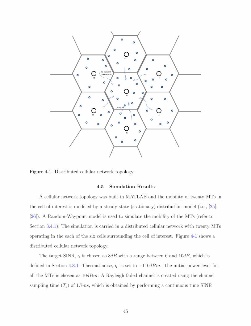
Figure 4-1. Distributed cellular network topology.
4.5 Simulation Results
A cellular network topology was built in MATLAB and the mobility of twenty MTs in
the cell of interest is modeled by a steady state (stationary) distribution model (i.e., [25],
[26]). A Random-Waypoint model is used to simulate the mobility of the MTs (refer to
Section 3.4.1). The simulation is carried in a distributed cellular network with twenty MTs
operating in the each of the six cells surrounding the cell of interest. Figure 4-1 shows a
distributed cellular network topology.
The target SINR, γ is chosen as 8dB with a range between 6 and 10dB, which is
defined in Section 4.3.1. Thermal noise, η, is set to −110dBm. The initial power level for
all the MTs is chosen as 10dBm. A Rayleigh faded channel is created using the channel
sampling time (Ts) of 1.7ms, which is obtained by performing a continuous time SINR
45
200 400 600 800 1000 1200 1400 1600
−2
0
2
4
6
Iterations, l
SIN
R E
rror
, in
dB
SINR Error Plot. Maximum Doppler Frequency of MT = 4.11Hz
0 200 400 600 800 1000 1200 1400 1600 1800−130
−120
−110
−100
−90
−80
Iterations, l
Cha
nnel
Gai
n, in
dB
Channel Gain Plot
0 200 400 600 800 1000 1200 1400 1600 1800−60
−40
−20
0
20
Iterations, l
Pow
er, i
n dB
m
Power Plot
Figure 4-2. Error, channel gain, and power plot of a MT with maximum Dopplerfrequency 4.11 Hz.
error analysis (see Section 3.3), and the Doppler frequency Equation 2–6. The prediction
observation sampling rate (Tp) is also chosen to be 1.7ms. The velocity for each of the
MTs is obtained from Equation 3–29. The angle θ is measured periodically and the
Doppler frequency is obtained from Equation 3–29 and Equation 2–6, which is used to
update the coefficients of the LMMSE predictor. Path loss, with free space propagation
effects (near-field effects), and log-normal shadowing are modelled [19] as shown in
Equation 2–1 and Equation 2–2.
The results in Figures 4-2 through 4-5 are obtained with
kn = 0.00005, kp = 1.6, ke = 0.00008,
and the spreading factor a is chosen as 156. The number of samples used for prediction
is 5. Figure 4-2 shows the SINR error, channel gain and power plots of a MT operating
around a maximum doppler frequency of 4.11Hz. The prediction error for this MT is
46
0 200 400 600 800 1000 1200 1400 1600 1800−3
−2.5
−2
−1.5
−1
−0.5
0
0.5
1
1.5
Iterations, l
Pre
dict
ion
Err
or, i
n dB
Prediction Error Plot
Figure 4-3. Prediction error of the MT with maximum Doppler frequency 4.11 Hz.
0 200 400 600 800 1000 1200 1400 1600 1800−30
−20
−10
0
10
20
Iterations, l
SIN
R E
rror
, in
dB
SINR Error Plot. Maximum Doppler Frequency of MT = 30.88Hz
0 200 400 600 800 1000 1200 1400 1600 1800−160
−140
−120
−100
−80
Iterations, l
Cha
nnel
Gai
n, in
dB
Channel Gain Plot
0 200 400 600 800 1000 1200 1400 1600 1800−40
−20
0
20
Iterations, l
Pow
er, i
n dB
m
Power Plot
Figure 4-4. Error, channel gain, and power plot of a MT with maximum Dopplerfrequency 30.9 Hz.
47
0 200 400 600 800 1000 1200 1400 1600 1800−25
−20
−15
−10
−5
0
5
10
15
20
Iterations, l
Pre
dict
ion
Err
or, i
n dB
Prediction Error Plot
Figure 4-5. Prediction error of the MT with maximum Doppler frequency 30.9 Hz.
shown in Figure 4-3. It can be seen that the power controller regulates the SINR of the
MT in the desired range almost perfectly. Figure 4-4 shows the SINR error, channel gain
and power plots of a MT operating around a maximum doppler frequency of 30.88Hz.
The prediction error for this MT is shown in Figure 4-5. The inaccurate prediction of the
linear predictor in the deep faded zones causes outage to the MT in those zones (Figures
4-4 and 4-5). The SINR of this radio link operating around a maximum doppler frequency
of 30.88Hz is in the acceptable communication range at all other times, and the power
required to achieve this is in the implementable range, well below the maximum power of
27dBm (500mW ) of MTs.
Table 4-1 shows the statistics of the SINR error of all the MTs in the cell of
importance. The second column of Table 4-1 quantifies the percentage of samples that
lie within the desired SINR range for each Doppler frequency. When samples exceed the
upper limit of the desired SINR range (i.e., xi(l) ≥ γmax), the quality of service for the
48
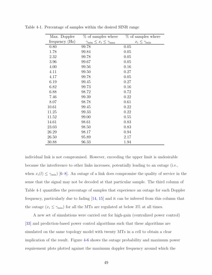
Table 4-1. Percentage of samples within the desired SINR range
Max. Dopplerfrequency (Hz)
% of samples whereγmin ≤ xi ≤ γmax
% of samples wherexi ≤ γmin
0.80 99.78 0.051.78 99.84 0.052.32 99.78 0.053.96 99.67 0.054.00 99.56 0.164.11 99.50 0.274.17 99.78 0.056.19 99.45 0.276.82 99.73 0.166.88 98.72 0.727.46 99.39 0.228.07 98.78 0.61
10.61 99.45 0.2211.25 99.33 0.2211.52 99.00 0.5514.61 98.61 0.8323.03 98.50 0.8326.29 98.17 0.9426.50 95.89 2.1730.88 96.33 1.94
individual link is not compromised. However, exceeding the upper limit is undesirable
because the interference to other links increases, potentially leading to an outage (i.e.,
when xi(l) ≤ γmin) [6–8]. An outage of a link does compromise the quality of service in the
sense that the signal may not be decoded at that particular sample. The third column of
Table 4-1 quantifies the percentage of samples that experience an outage for each Doppler
frequency, particularly due to fading [14, 15] and it can be inferred from this column that
the outage (xi ≤ γmin) for all the MTs are regulated at below 3% at all times.
A new set of simulations were carried out for high-gain (centralized power control)
[33] and prediction-based power control algorithms such that these algorithms are
simulated on the same topology model with twenty MTs in a cell to obtain a clear
implication of the result. Figure 4-6 shows the outage probability and maximum power
requirement plots plotted against the maximum doppler frequency around which the
49
0 5 10 15 20 25 30 3510
−4
10−3
10−2
10−1
100
Outage Probability Vs Maximum Doppler Frequency of MTs
Maximum Doppler Frequency (Hz)
Out
age
Pro
babi
lity
0 5 10 15 20 25 30 35
10
15
20
25
27
30Maximum Power Level Vs Maximum Doppler Frequency of MTs
Maximum Doppler Frequency (Hz)
Max
imum
Pow
er (
dBm
)
1 Prediction Sample3 Prediction Samples5 Prediction SamplesHigh−Gain (No Prediction)
Figure 4-6. Comparison of high gain and predictive power control algorithms.
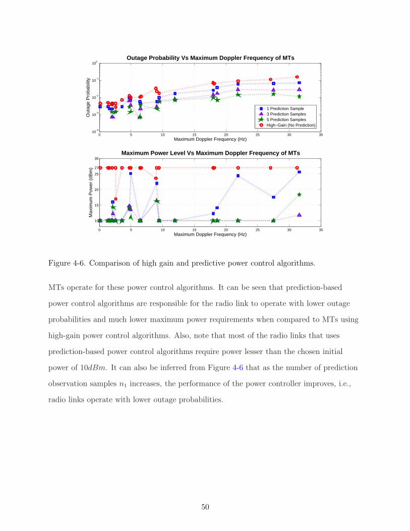
MTs operate for these power control algorithms. It can be seen that prediction-based
power control algorithms are responsible for the radio link to operate with lower outage
probabilities and much lower maximum power requirements when compared to MTs using
high-gain power control algorithms. Also, note that most of the radio links that uses
prediction-based power control algorithms require power lesser than the chosen initial
power of 10dBm. It can also be inferred from Figure 4-6 that as the number of prediction
observation samples n1 increases, the performance of the power controller improves, i.e.,
radio links operate with lower outage probabilities.
50
CHAPTER 5CONCLUSION
5.1 Summary of Results
Radio channel uncertainties, particularly fading, are responsible for the cellular
network to be characterized as a nonlinear system. The fading process is characterized
as a time-varying stochastic process which is responsible for significant power drops in
certain regions known as deep faded regions causing problems in recovering the signal
at the receiver. Further, restrictions in the maximum power at which the signals can be
transmitted in such systems and bandwidth availability intensifies the need to develop
power controllers for such radio links. To address these problems, controllers are designed
that uses the Lyapunov-based tools to analyze the nonlinear system, and the simulation
results are discussed to demonstrate and validate the theory behind the control design.
In Chapter 3, a robust power controller is developed for a wireless CDMA-based
cellular network system. Lyapunov-based stability analysis is used to develop an ultimate
bound for the sampled SINR error which can be decreased up to a point by increasing a
nonlinear damping gain. An analysis is also provided to illustrate how mobility and the
desired SINR regulation range affects the choice of channel update times. The choice of
the update time also affects the ultimate bound that the sampled SINR error reaches -
Lowering the sampling time reduces the ultimate bound. Simulations indicate that the
SINRs of radio links operating with lower maximum Doppler frequency are maintained in
the desired communication range. Radio links operating with a high maximum Doppler
frequency have high outage probability due to the fastly time-varying nature of the
channel uncertainties, and this motivated to use the concept of prediction to address the
issue.
Chapter 4 introduces a MMSE prediction-based power control algorithm for a wireless
CDMA-based distributed cellular networked system. A linear predictor is used to predict
the fading power at the l + 1 th instant, and this information is fed to the controller from
51

which the power update law is obtained, which in this case is logarithmic in operation
unlike the proportional controller developed in Chapter 3. A Lyapunov-based analysis is
used to develop an ultimate bound for the sampled SINR error which can be decreased
up to a point by increasing a nonlinear damping gains. Simulations indicate that the
SINRs of all the radio links are regulated in the region γmin ≤ xi(·) ≤ γmax with a
outage probability of less than 3%. Local SINR measurements are used to simulate the
distributed cellular network. Outages at some regions were determined to be due to
limitations of the linear predictor, especially in the deep faded zones.
5.2 Recommendations for Future Work
In order to improve to performance of the controller designed in Chapter 4, more
sophisticated prediction and control development concepts are required in such highly
time-varying radio channels as encountered in the fading radio channels of urban
environments. Wiener filters and other Lyapunov-based adaptive control development
techniques can be used to improve the quality of service for cellular communication
networks. Optimal control development for such nonlinear stochastic radio channels can
potentially enhance the radio link quality of cellular communication networks.
The modeling and the control development methodologies followed in this work
can be extended to wireless Mobile Ad-Hoc Networks (MANETs), where in addition
to the random time-varying phenomena in the radio channel, unpredictable topological
changes, bandwidth and power constraints, multiuser interference, time-delays (due to
contention, back-off, etc), link scheduling and routing are some of the additional challenges
encountered. Modeling and embedding such factors experienced in MANETs in the system
model developed in this thesis for developing power control algorithms, and optimizing its
performance based on the constraints in MANETs is potentially the next goal in this line
of research.
52
APPENDIX AESTIMATION OF RANDOM PROCESSES
A-1 General MMSE based estimation theory
Let W (l) be some random process that needs to be estimated. The problem of finding
the estimates of the zero mean gaussian random variables can be defined as follows.
ε2min = min
W (l)E
[
(
W (l) − W (l))2]
given W (l − 1), W (l − 2), W (l − 3), ..
= minW (l)
E[(
W 2(l) − 2W (l)W (l) + W 2(l))]
given W (l − 1), W (l − 2), W (l − 3), ..
= minW (l)
E[
W 2(l)]
− 2W (l)E [W (l)] + W 2(l) given W (l − 1), W (l − 2), W (l − 3), .. (A-1)
To find the minimum value of the estimate of W ,
d
dW (l)
E[
W 2(l)]
− 2W (l)E [W (l)]
= 0 given W (l − 1), W (l − 2), W (l − 3), ..
=⇒ 0 − 2E [W (l)] + 2W (l) = 0 given W (l − 1), W (l − 2), W (l − 3), ..
The estimate is given by [34]
W (l) = E [W (l) | W (l − 1), W (l − 2), W (l − 3), ..] , (A-2)
The conditional estimate is given by
E [W (l) | W (l − 1), W (l − 2), W (l − 3), ..] ,
where W (l), W (l − 1), W (l − 2), W (l − 3), .. are all jointly gaussian and W (l − 1), W (l −
2), W (l−3), .... are the past values of the random variable W that are used to estimate the
current value W (l).
53
A-2 Gaussian Case
The conditional probability density function is given by [36]
fW (l) [W (l) | W (l − 1), W (l − 2), W (l − 3), ..]
=fW (l),W (l−1),W (l−2),... [W (l), W (l − 1), W (l − 2), W (l − 3), ..]
fW (l−1),W (l−2),... [W (l − 1), W (l − 2), W (l − 3), ..], (A-3)
where the numerator and denominator are joint density functions of the zero-mean
gaussian random variables W upto instants l and l − 1 respectively. The Covariance
Matrices Kn and Kn−1 are defined as follows
Kn = E[
[Yl] . [Yl]T]
,
and Kn−1 = E[
[Yl−1] . [Yl−1]T]
,
where
Yl =
[
W (l − s) W (l − (s − 1)) . . W (l)
]T
,
and Yl−1 =
[
W (l − s) W (l − (s − 1)) . W (l − 1)
]T
.
Since the means of the random variables W are zero at any l
fW (l) [W (l) | W (l − 1), W (l − 2), W (l − 3), ..]
=exp
−12Y T
l K−1n Yl
(2π)n
2 |Kn|1/2
.
exp
−12Y T
l−1K−1n−1Yl−1
(2π)(n−1)
2 |Kn−1|1/2
−1
. (A-4)
Since W (l) is a zero-mean gaussian random process, the MMSE estimate is a linear
estimate, i.e., E [W (l) | W (l − 1), W (l − 2), W (l − 3), ..] can be obtained by manipulating
Equation A-4. For a simple case with only one given value, the linear MMSE estimation is
54
given by
E [W (l) | W (l − 1)]
= µW (l) + ρW (l)W (l−1)
(
σW (l)
σW (l−1)
)
(
W (l − 1) − µW (l−1)
)
=
[
ρW (l)W (l−1)
(
σW (l)
σW (l−1)
)]
W (l − 1), (A-5)
where ρW (l)W (l−1) is the autocorrelation function, σW (l) and σW (l−1) are the variances.
55
APPENDIX BORTHOGONALITY CONDITION
Let Y , X1, X2, X3, ...., XN be gaussian random variables with zero means. The
MMSE estimate is the conditional mean, given by
E [Y | X1,X2, X3, ...., XN ] =
N∑
k=1
aiXi. (B-1)
The random variables
(
Y −N∑
k=1
aiXi
)
, X1, X2, X3, ...., XN are jointly gaussian. Since
the first term is uncorrelated with all the rest, it can be inferred that the random variable(
Y −N∑
k=1
aiXi
)
is uncorrelated with X1, X2, X3, ...., XN . Therefore,
E
[(
Y −
N∑
k=1
aiXi
)
| X1,X2, X3, ...., XN
]
= E
[(
Y −
N∑
k=1
aiXi
)]
= E [Y ] −
N∑
k=1
aiE [Xi] = 0,
since E [Y ] = E [Xi] = 0. The condition
E
[(
Y −N∑
k=1
aiXi
)
| X1,X2, X3, ...., XN
]
= 0 (B-2)
is known as the Orthogonality Condition, which can also be written as
[
Y − aT X]
⊥ X, (B-3)
where
X =
[
X1 X2 . . XN
]T
.
The ai’s can be obtained from the orthogonality condition.
Note: From Equation B-2, we get
E [Y | X1,X2, X3, ...., XN ] −
N∑
k=1
aiE [Xi | X] = 0.
56
=⇒ E [Y | X1,X2, X3, ...., XN ] −
N∑
k=1
aiXi = 0
=⇒ E [Y | X1,X2, X3, ...., XN ] =
N∑
k=1
aiXi. (B-4)
Thus, the conditional mean of a zero-mean gaussian random variable Y is given by a linear
estimate of the given variables Xis.
Calculation of ai’s.
From the Orthogonality condition in Equation B-2, we get [34]
E
[(
Y −N∑
k=1
aiXi
)
| Xp
]
= 0, 1 ≤ p ≤ k
=⇒ E [Y Xp] =
N∑
k=1
aiE [XkXp] , 1 ≤ p ≤ k.
=⇒ kY X = aT KY Y , (B-5)
where
a ,
[
a1 a2 . . aN
]T
,
kY X ,
[
E [Y X1] E [Y X2] E [Y X3] . . E [Y XN ]
]
=
[
KY X1 KY X2 KY X3 . . KY XN
]
,
and the covariance matrix
KXX = E[
XXT]
. (B-6)
From Equation B-5, we get
aT = kY XKTXX . (B-7)
57
REFERENCES
[1] N. Bambos, S. Chen, and G. Pottie, “Channel access algorithms with active linkprotection for wireless communication networks with power control,” IEEE/ACMTrans. Networking, no. 5, pp. 583–597, 2000.
[2] G. Foschini and Z. Miljanic, “A simple distributed autonomous power controlalgorithm and its convergence,” IEEE Tran. Veh. Technol., vol. 42, pp. 641–646, 1993.
[3] S. Grandhi and J. Zander, “Constrained power control in cellular radio systems,” inVehicular Technology Conference, 1994 IEEE 44th, 8-10 June 1994, pp. 824–828vol.2.
[4] R. Jantti and S. Kim, “Second-order power control with asymptotically fastconvergence,” IEEE J. Select. Commun, vol. 18, no. 3, 2000.
[5] R. D. Yates, “A framework for uplink power control in cellular radio systems,” IEEEJ. Select. Areas Commun., vol. 13, pp. 1341–1347, Sept. 1995.
[6] J. Zander, “Optimum global transmitter power control in cellular radio systems,” inIEEE Int. Symp. on Personal, Indoor and Mobile Radio Commun., London, U.K.,1991.
[7] ——, “Distributed cochannel interference control in cellular radio systems,” IEEETran. Veh. Technol., vol. 41, pp. 305–311, 1992.
[8] ——, “Performance of optimum transmitter power control in cellular radio systems,”IEEE Trans. Veh. Technol., vol. 41, pp. 57–62, 1992.
[9] J. Aein, “Power balancing in systems employing frequency reuse,” COMSAT Tech.Rev., pp. 277–299, 1973.
[10] H. Alavi and R. Nettleton, “Downstream power control for a spread spectrum cellularmobile radio system,” in Proc. IEEE GLOBECOM, 1982, pp. 84–88.
[11] S. Grandhi, R. Vijayan, and J. Zander, “Centralized power control in cellular radiosystems,” IEEE Transactions on Vehicular Technology, vol. 42, no. 4, November 1993.
[12] R. D. Yates and C. Y. Huang, “Integrated power control and base stationassignment,” IEEE Trans. Veh. Technol., vol. 44, pp. 638–644, Aug. 1995.
[13] S. Dontula and S. Jagannathan, “Active link protection for wireless peer-to-peer andcellular networks with power control,” in World Wireless Congress, 2004, pp. 612–617.
[14] S. Kandukuri and S. Boyd, “Optimal power control in interference-limited fadingwireless channels with outage-probability specifications,” IEEE Transactions onWireless Communications, vol. 1, no. 1, pp. 46–55, January 2002.
[15] J. Papandriopoulos, J. Evans, and S. Dey, “Optimal power control for Rayleigh-fadedmultiuser systems with outage constraints,” IEEE Transactions on Wireless Commu-nications, vol. 4, no. 6, pp. 2705–2715, November 2005.
58
[16] S. Jagannathan, Wireless Ad Hoc and Sensor Networks, F. L. Lewis, Ed. CRC Press,2007.
[17] S. Jagannathan, M. Zawodniok, and Q. Shang, “Distributed power control for cellularnetworks in the presence of channel uncertainties,” IEEE Transactions on WirelessCommunications, vol. 5, no. 3, 2006.
[18] R. Canchi and Y. Akaiwa, “Performance of adaptive transmit power control inπ/4 DQPSK mobile radio systems in flat Rayleigh fading channels,” in VehicularTechnology Conference, 1999 IEEE 49th, vol. 2, 16-20 May 1999, pp. 1261–1265vol.2.
[19] T. Rappaport, Wireless Communications, Principles and Practice. Prentice Hall,1999.
[20] L. Gao and T. Wong, “Power control and spreading sequence allocation in a cdmaforward link,” IEEE Trans. Inform. Theory, vol. 50, no. 1, pp. 105–124, Jan. 2004.
[21] N. Bambos, “Towards power-sensitive network architechtures in wirelesscommunications: Concepts, issues and design aspects,” IEEE Pers. Commun.,pp. 50–59, 1998.
[22] A. J. Viterbi, CDMA: Principles of Spread Spectrum Communication. AddisonWesley, 1995.
[23] R. H. Clarke, “A statistical theory of mobile-radio reception,” Bell Syst. Technical J.,vol. 47, no. 6, pp. 957–1000, Jul.–Aug. 1968.
[24] J. Spooner, M. Maggiore, R. Ordonez, and K. Passino, Stable Adaptive Control andEstimation for Nonlinear Systems. Wiley, 2002.
[25] S. PalChaudhuri, J.-Y. Le Boudec, and M. Vojnovic, “Perfect simulations for randomtrip mobility models,” in Simulation Symposium, 2005. Proceedings. 38th Annual, 4-6April 2005, pp. 72–79.
[26] J.-Y. Le Boudec and M. Vojnovic, “Perfect simulation and stationarity of a class ofmobility models,” in INFOCOM 2005. 24th Annual Joint Conference of the IEEEComputer and Communications Societies. Proceedings IEEE, vol. 4, 13-17 March2005, pp. 2743–2754vol.4.
[27] A. Duel-Hallen, S. Hu, and H. Hallen, “Long range prediction of fading signals:Enabling adaptive transmission for mobile radio channels,” IEEE Signal ProcessingMag., vol. 17, no. 3, pp. 62–75, May 2000.
[28] T. Eyceoz, A. Duel-Hallen, and H. Hallen, “Deterministic channel modeling and longrange prediction of fast fading mobile radio channels,” IEEE Commun. Lett., vol. 2,no. 9, pp. 254–256, Sept. 1998.
59
[29] T. Eyceoz, S. Hu, and A. Duel-Hallen, “Performance analysis of long range predictionfor fast fading channels,” in Proc. of 33rd Annual Conf. on Inform. Sciences andSystems CISS99, vol. II, Mar. 1999, pp. 656 – 661.
[30] S. Hu, H. Hallen, and A. Duel-Hallen, “Physical channel modeling, adaptiveprediction and transmitter diversity for flat fading mobile channel,” in Signal Pro-cessing Advances in Wireless Communications, 1999. SPAWC ’99. 1999 2nd IEEEWorkshop on, 9-12 May 1999, pp. 387–390.
[31] S. Hu, T. Eyceoz, A. Duel-Hallen, and H. Hallen, “Transmitter antenna diversity andadaptive signaling using long range prediction for fast fading DS/CDMA mobile radiochannels,” in Wireless Communications and Networking Conference, 1999. WCNC.1999 IEEE, 21-24 Sept. 1999, pp. 824–828vol.2.
[32] T. Eyceoz, S. Hu, A. Duel-Hallen, and H. Hallen, “Adaptive prediction, tracking andpower adjustment for frequency non-selective fast fading channels,” in CommunicationTheory Mini-Conference, 1999, 6-10 June 1999, pp. 1–5.
[33] S. Subramanian, J. M. Shea, and W. E. Dixon, “Power control of cellularcommunications with channel uncertainties,” in American Control Conference,2009. ACC ’09, 2009, to appear.
[34] H. Stark and J. W. Woods, Probability and Random Processes with Applications toSignal Processing, 3rd ed. Pearson Education, 2002.
[35] W. C. Jakes, Microwave Mobile Communications. Wiley, 1974.
[36] A. Leon-Garcia, Probability and Random Processes for Electrical Engineering, 2nd ed.Addison Wesley, 1994.
60
BIOGRAPHICAL SKETCH
Sankrith Subramanian was born in Chennai, India in 1985. He received his bachelor’s
degree in instrumentation and control engineering from St. Joseph’s College of Engineering
(Anna University), Chennai, India in May 2006. He received his Master of Science degree
from the University of Florida in 2009. His interests lie in the field of networked control
systems, nonlinear controls, wireless communication, signal processing and automation.
Sankrith pursued his Master of Science degree in the Department of Electrical and
Computer Engineering and was a graduate research assistant in the Nonlinear Controls
and Robotics group in the Department of Mechanical and Aerospace Engineering at the
University of Florida, under the supervision of Dr. Warren E. Dixon. He was co-advised
by Dr. John M. Shea of the Wireless Information Networking Group in the Department of
Electrical and Computer Engineering at the University of Florida.
The primary focus of his research was to analyze wireless CDMA-based cellular
communication networks with time-varying stochastic channel uncertainties and design
Lyapunov-based nonlinear power controllers. Simulation demonstrations were provided
with the help of realistic network topology models. His future interest is to extend and
apply his research to wireless ad-hoc networks.
61


