

PPTs onProbability Theory and Stochastic Process
B.TECH III SEM-ECEIARE-R16
By
– Mrs. G Ajitha, Assistant Professor– Dr. M V Krishna Rao, Professor– Mr. N Nagaraju, Assistant Professor– Mr. G. Anil Kumar Reddy, Assistant Professor
1

UNIT-IProbability and Random Variable
2

Introduction to Set
• Set: A set is a well defined collection of objects. These objects arecalled elements or members of the set. Usually uppercase letters areused to denote sets.
• The set theory was developed by George Cantor in 1845-1918. Today,it is used in almost every branch of mathematics and serves as afundamental part of present-day mathematics.
• In everyday life, we often talk of the collection of objects such as abunch of keys, flock of birds, pack of cards, etc.
• In mathematics, we come across collections like natural numbers,whole numbers, prime and composite numbers.
3
Laws in set theory
• A∩B = B∩A (Commutative law)
• (A∩B)∩C = A∩ (B∩C) (Associative law)
• Ф ∩ A = Ф (Law of Ф)
• U∩A = A (Law of ∪)
• A∩A = A (Idempotent law)
• A∩(B∪C) = (A∩B) ∪ (A∩C) (Distributive law) Here ∩ distributes over ∪
• Also, A∪(B∩C) = (AUB) ∩ (AUC) (Distributive law) Here ∪ distributes over ∩
4
Probability
• Experiment:
In probability theory, an experiment or trial (see below) is anyprocedure that can be infinitely repeated and has a well-defined setof possible outcomes, known as the sample space.
• An experiment is said to be random if it has more than one possibleoutcome, and deterministic if it has only one.
• A random experiment that has exactly two (mutually exclusive)possible outcomes is known as a Bernoulli trial.
5

Experiment
6

Random Experiment
• An experiment is a random experiment if its outcome cannot bepredicted precisely. One out of a number of outcomes is possible ina random experiment.
• A single performance of the random experiment is called atrial.Random experiments are often conducted repeatedly, so thatthe collective results may be subjected to statistical analysis.
• A fixed number of repetitions of the same experiment can bethought of as a composed experiment, in which case the individualrepetitions are called trials.
• For example, if one were to toss the same coin one hundred timesand record each result, each toss would be considered a trial withinthe experiment composed of all hundred tosses.
7

• Relative Frequency:
Random experiment with sample space S. we shall assign non-negative number called probability to each event in the sample space.Let A be a particular event in S. then “the probability of event A” isdenoted by P(A).
• Suppose that the random experiment is repeated n times, if the eventA occurs nA times, then the probability of event A is defined as“Relative frequency
• Event A is defined as
Relative frequency, Experiments
8

Sample Space
• Sample Space: The sample space is the collection of all possibleoutcomes of a random experiment. The elements of are calledsample points. A sample space may be finite, countable infinite oruncountable.
• A list of exhaustive *don’t leave anything out] and mutuallyexclusive outcomes [impossible for 2 different events to occur inthe same experiment] is called a sample space and is denoted by S.
• The outcomes are denoted by O1, O2, …, Ok
• Using notation from set theory, we can represent the sample spaceand its outcomes as:
S = {O1, O2, …, Ok}
9

Sample Space
• Given a sample space S = {O1, O2, …, Ok}, the probabilities assigned to the outcome must satisfy these requirements:
(1) The probability of any outcome is between 0 and 1
i.e. 0 ≤ P(Oi) ≤ 1 for each i, and
(2) The sum of the probabilities of all the outcomes equals 1
i.e. P(O1) + P(O2) + … + P(Ok) = 1
10

Discrete and Continuous Sample Spaces
• Probability assignment in a discrete sample space: Consider a finitesample space . Then the sigma algebra is defined by the power set ofS. For any elementary event , we can assign a probability such that,For any event , we can define the probability
11

Continuous sample space
• Suppose the sample space S is continuous and uncountable. Such asample space arises when the outcomes of an experiment arenumbers. For example, such sample space occurs when theexperiment consists in measuring the voltage, the current or theresistance.
12

Events
• The probability of an event is the sum of the probabilities of thesimple events that constitute the event.
• E.g. (assuming a fair die) S = {1, 2, 3, 4, 5, 6} and P(1) = P(2) = P(3) =P(4) = P(5) = P(6) = 1/6
• Then: P(EVEN) = P(2) + P(4) + P(6) = 1/6 + 1/6 + 1/6 = 3/6 = 1/2
13
Types of Events
1. Exhaustive Events:
A set of events is said to be exhaustive, if it includes all the possibleevents. Ex. In tossing a coin, the outcome can be either Head or Tailand there is no other possible outcome. So, the set of events{ H , T }is exhaustive.
2. Mutually Exclusive Events:
Two events, A and B are said to be mutually exclusive if they cannotoccur together. i.e. if the occurrence of one of the events precludesthe occurrence of all others, then such a set of events is said to bemutually exclusive. If two events are mutually exclusive then theprobability of either occurring is
14

Types of Events
3. Equally Likely Events:
If one of the events cannot be expected to happen in preference toanother, then such events are said to be Equally Likely Events.( Or)Each outcome of the random experiment has an equal chance ofoccurring.
Ex. In tossing a coin, the coming of the head or the tail is equallylikely
4. Independent Events:
Two events are said to be independent, if happening or failureof one does not affect the happening or failure of the other.Otherwise, the events are said to be dependent.
15

Probability Definitions and Axioms
Relative frequency Definition:
Consider that an experiment E is repeated n times, and let A and B betwo events associated with E. Let nA and nB be the number of timesthat the event A and the event B occurred among the n repetitionsrespectively. The relative frequency of the event A in the 'n'repetitions of E is defined as
f( A) = nA /n
16

Axioms of Probability
• The Relative frequency has the following properties:
• 0 ≤f(A) ≤ 1
• f(A) =1 if and only if A occurs every time among the n repetitions.
• If an experiment is repeated n times under similar conditions and the event A occurs in nAtimes, then the probability of the event A is defined as
17

Joint probability
• Joint probability:
Joint probability is defined as the probability of both A and B taking place, and is denoted by P (AB) or P(A∩B) .
• probability notation: P(AB) = P(A | B) * P(B)
18

Conditional Probability
• Conditional probability is used to determine how two events arerelated; that is, we can determine the probability of one event giventhe occurrence of another related event.
• Experiment: random select one student in class.
• P(randomly selected student is male)
• P(randomly selected student is male/student is on 3rd row)
• Conditional probabilities are written as P(A | B) and read as “theprobability of A given B” and is calculated as
19

Bayes’ Theorem
• Bayes’ Law is named for Thomas Bayes, an eighteenth centurymathematician.
• In its most basic form, if we know P(B | A),
• we can apply Bayes’ Law to determine P(A | B)
• Bayes' theorem centers on relating different conditionalprobabilities. A conditional probability is an expression of howprobable one event is given that some other event occurred(a fixed value).
• For a joint probability distribution over events A and B ,P(A^B), the conditional probability of given is defined as
20

Bayes’ theorem
• Note that P(A^B) is the probability of both A and B occurring, whichis the same as the probability of A occurring times the probabilitythat B occurs given that A occurred P(B/A)*P(A)• Using the same reasoning P(A^B), is also the probability that Boccurs times the probability that A occurs given that B occurs:P(A/B)*P(B) The fact that these two expressions are equal leads toBayes' Theorem. Expressed mathematically, this is:
21

• The probabilities P(A) and P(AC) are called prior probabilitiesbecause they are determined prior to the decision about taking thepreparatory course.
• The conditional probability P(A | B) is called a posterior probability(or revised probability), because the prior probability is revisedafter the decision about taking the preparatory course.
Bayes’ theorem
22

Random variable
• A (real-valued) random variable, often denoted by X (or some othercapital letter), is a function mapping a probability space (S, P) intothe real line R. This is shown in next slide.
• Associated with each point s in the domain S the function X assignsone and only one value X(s) in the range R. (The set of possiblevalues of X(s) is usually a proper subset of the real line; i.e., not allreal numbers need occur. If S is a finite set with m elements, thenX(s) can assume at most m different values as s varies in S.)
23

RV in graphical representation
24

RV in graphical representation
25
Discrete random variable
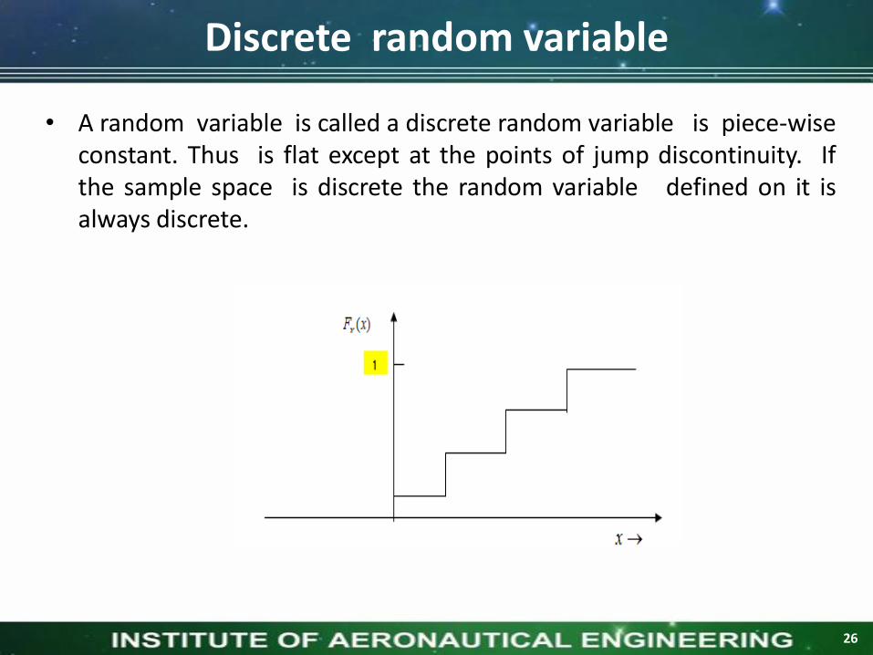
• A random variable is called a discrete random variable is piece-wiseconstant. Thus is flat except at the points of jump discontinuity. Ifthe sample space is discrete the random variable defined on it isalways discrete.
26

Continuous random variable
• X is called a continuous random variable if is an absolutely continuousfunction of x. Thus is continuous everywhere on and existseverywhere except at finite or countable infinite points.
27
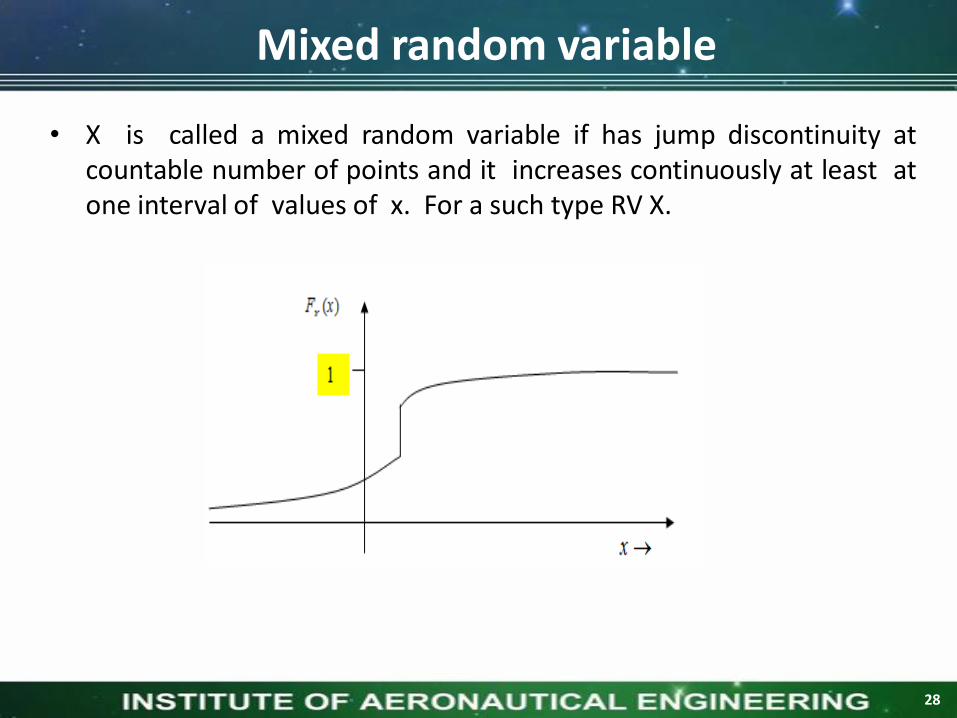
Mixed random variable
• X is called a mixed random variable if has jump discontinuity atcountable number of points and it increases continuously at least atone interval of values of x. For a such type RV X.
28

UNIT-IIDistribution and Density Functions
29

Random Variable
Review of the concepts1. Random Experiment2. Random Event 3. Outcomes4. Sample Space5. Random Variable:
Mapping of sample space to a real line
30

Mapping of sample space to a real line
Random Variable
31

Distribution function
32
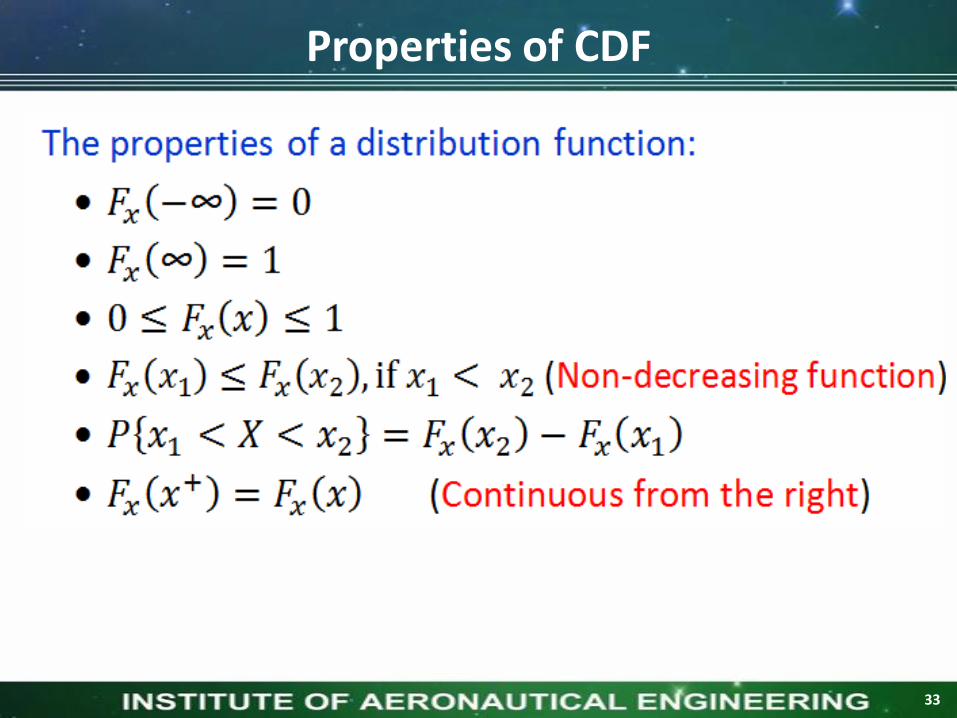
Properties of CDF
33

Properties of CDF (contd..)
34

Properties of CDF (contd..)
35

Probability density function
36

Probability density function (contd..)
37
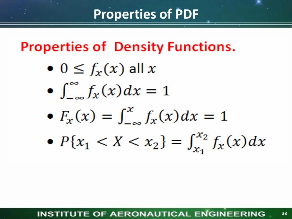
Properties of PDF
38

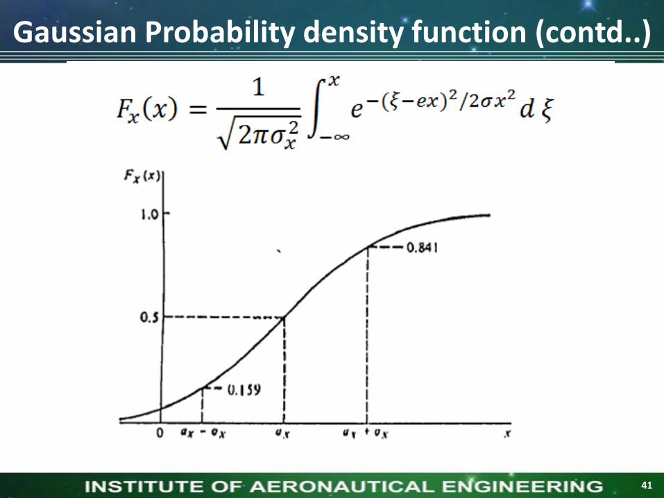
Gaussian Probability density function
39

Gaussian Probability density function (contd..)
40
Gaussian Probability density function (contd..)
41

Gaussian Probability density function (contd..)
42

Gaussian Probability density function (contd..)
43

Binomial Probability density function
44
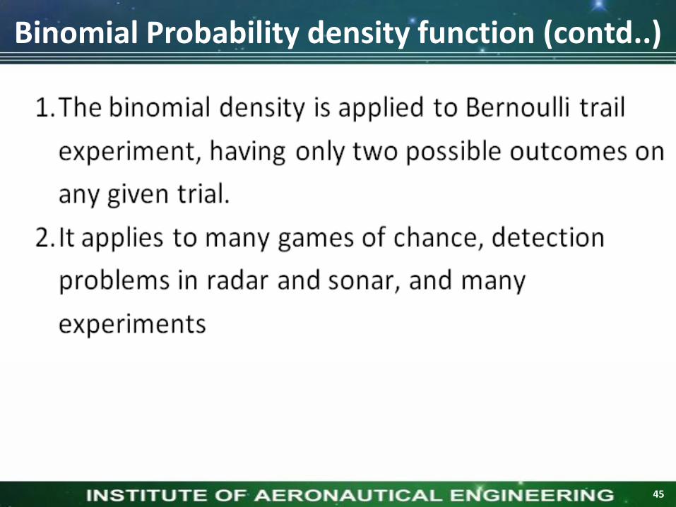
Binomial Probability density function (contd..)
45
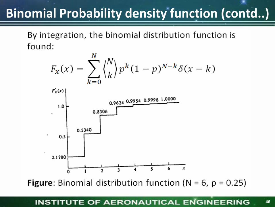
Binomial Probability density function (contd..)
46

Poisson Probability density function
47

Poisson Probability density function (contd..)
48
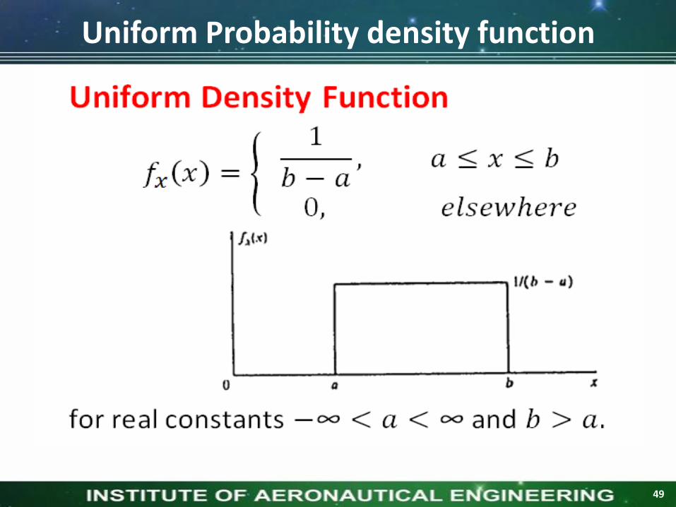
Uniform Probability density function
49

Uniform Probability density function (contd..)
50

Uniform Probability density function (contd..)
51

Exponential Probability density function
52
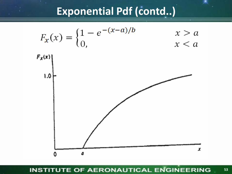
Exponential Pdf (contd..)
53

Exponential Pdf (contd..)
54

Rayleigh Probability density function
55

Rayleigh Probability density function (contd..)
56

Rayleigh Probability density function (contd..)
57

Conditional distribution function
58

Properties of Conditional distribution function
59

Conditional density function
60
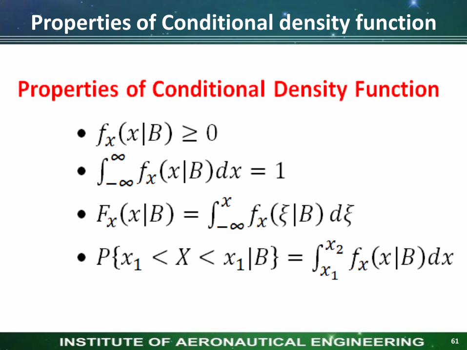
Properties of Conditional density function
61

Methods of conditioning event
62

Methods of conditioning event (contd..)
63

Methods of conditioning event (contd..)
64

Methods of conditioning event (contd..)
65

Methods of conditioning event (contd..)
66

Moments about origin
67
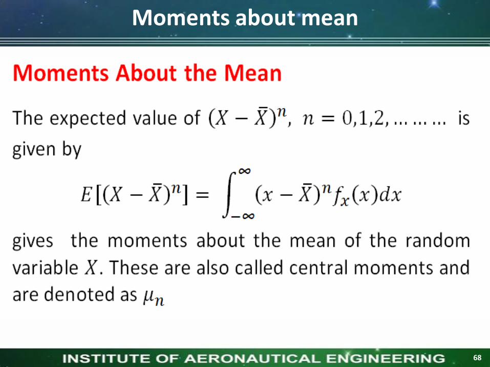
Moments about mean
68

Characteristic function
69

Moment generating function
70

Moment generating function
71

Monotonically increasing RV
72

Monotonically increasing RV (contd..)
73
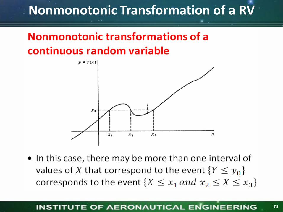
Nonmonotonic Transformation of a RV
74

Nonmonotonic Transformation of a RV (contd..)
75

Nonmonotonic Transformation of a RV (contd..)
76

Transformation of a DiscreteRV
77
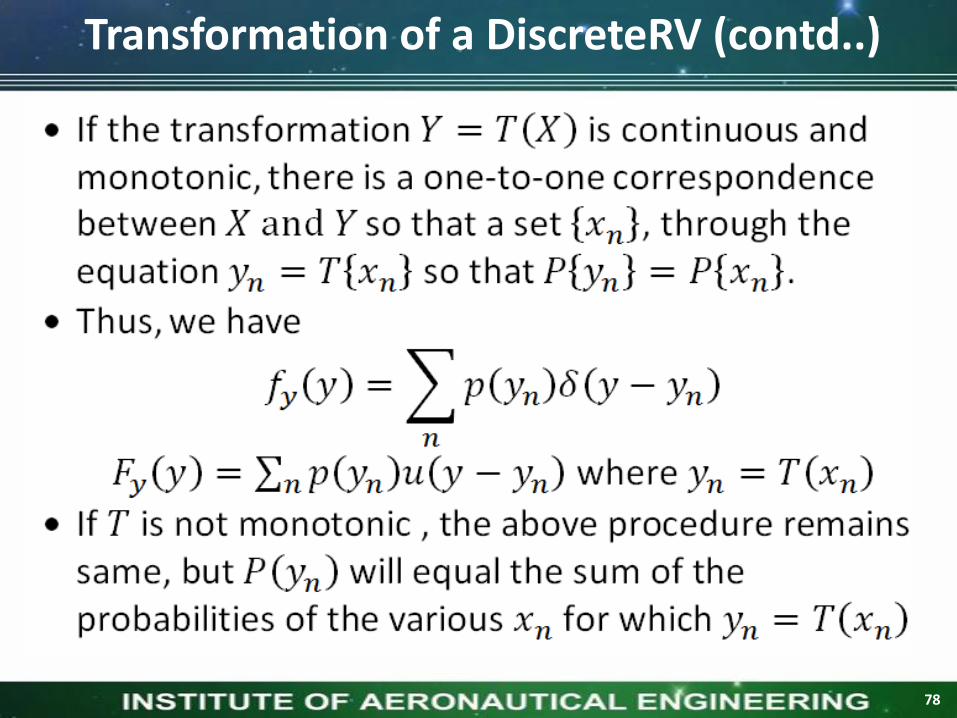
Transformation of a DiscreteRV (contd..)
78

Expected value of a RV
79
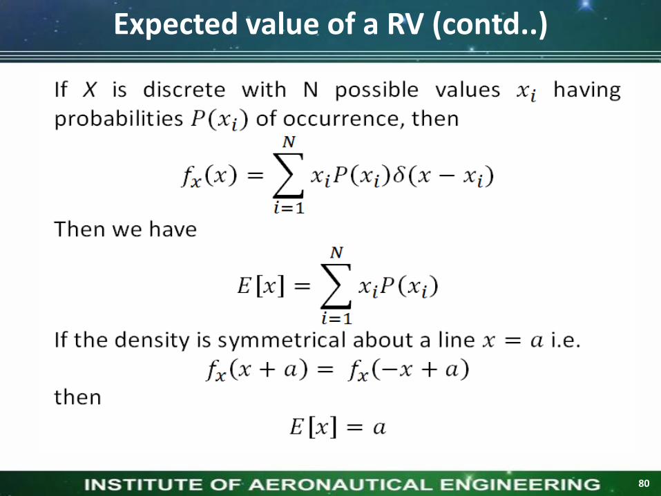
Expected value of a RV (contd..)
80

Conditional Expected value of a RV
81

Conditional Expected value of a RV (contd..)
82

Moments about origin
83

Moments about origin (contd..)
84

Moments about mean
85

Moments about mean (contd..)
86

Variance
87

Variance (contd..)
88

Skew
89

Skew (contd..)
90

UNIT-IIIMultiple Random Variables and
Operations
91

Vector random variables
• There are many cases where the outcome is a vector of numbers.We have already seen one such experiment, in, where a dart isthrown at random on a dartboard of radius r. The outcome is a pair(X, Y) of random variables that are such that X2 + Y2 ≤ r2.
• we measure voltage and current in an electric circuit with knownresistance. Owing to random fluctuations and measurement error,we can view this as an outcome (V, I)of a pair of random variables.
• Mapping the sample space to joint sample space
Comparision of sample space s with sj
92

Joint distribution function
• Let X and Y be random variables. The pair (X, Y) is then called a (two-dimensional) random vector.
• The joint distribution function (joint cdf) of (X, Y) is defined as F(x, y) = P(X ≤ x, Y ≤ y) for x, y ∈ R.
• Assume the joint sample space SJ has only three possible elements (1,1),(2,1),(3,3).The probabilities of the elements are to be P(1,1)=0.2,P(2,1)=0.3 ,P(3,3)=0.5.We find FX,Y(X,Y)
• In constructing joint distribution function we observe that has noelements for x<1,y<1.only at the point (1,1)does the function assumea step value.
• So long as x≥1,y≥1 this probability is maintained.For larger x and ythe point(2,1) produces a second stair step of 0.3 which holds theregion x≥2,y≥1.The second step is added to the first.Finally third stepof 0.5 is added to the two for x≥3,y≥3
93
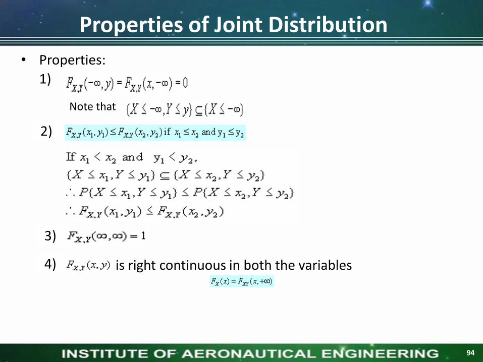
Properties of Joint Distribution
• Properties:
1)
Note that
2)
3)
is right continuous in both the variables4)
94

Properties of joint distribution
5)
6)
Called marginal cumulative distribution function
95

Marginal distribution functions
• The distribution of one random variable can be obtained by settingthe other value to infinity in FX,Y(x,y). The functions obtained in thismanner FX(x),FY(y) are called marginal distribution functions.
• Example:
FX,Y(x,y)=P(1,1)u(x-1)u(y-1)+P(2,1)u(x-2)u(y-1)+ P(3,3)u(x-3)u(y-3)
P(1,1)=0.2, P(2,1)=0.3, P(3,3)=0.5 if we set y=∞ then
FX(x)= 0.2u(x-1)+0.3u(x-2)+ 0.5u(x-3)
similarly
FY(y)= 0.2u(y-1)+0.3u(y-1)+ 0.5u(y-3)
=0.5u(y-1)+0.5u(y-3)
96

Marginal distribution functions
• Consider two jointly distributed random variables and with the joint CDF
1) Find the marginal CDFs
2) Find the probability P(1<x≤2, 1<y≤2)
2
,
(1 )(1 ) 0 , 0( , )
0 o th e rw ise
x y
X Y
e e x yF x y
97

Marginal distribution functions
a)2
,
,
1 0( ) lim ( , )
0 e ls e w h e re
1 y 0( ) lim ( , )
0 e ls e w h e re
x
X X Yy
y
Y X Yx
e xF x F x y
eF y F x y
, , , ,
4 2 2 1 2 2 4 1
{1 2 , 1 2} ( 2 , 2 ) (1,1) (1, 2 ) ( 2 ,1)
(1 )(1 ) (1 )(1 ) (1 )(1 ) (1 )(1 )
= 0 .0 2
X Y X Y X Y X YP X Y F F F F
e e e e e e e e
7 2
98

Joint Probability Density Function
• If and are two continuous random variables and their jointdistribution function is continuous in both and then we can definejoint probability density function by
provided it exists.
Clearly
2
, ,( , ) ( , ) ,
X Y X Yf x y F x y
x y
, ,( , ) ( , )
yx
X Y X YF x y f u v d vd u
99

Marginal density function
• The marginal CDF and pdf are same as the CDF and pdf of theconcerned single random variable. The marginal term simply refersthat it is derived from the corresponding joint distribution ordensity function of two or more jointly random variables.
• With the help of the two-dimensional Dirac Delta function, we candefine the joint pdf of two discrete jointly random variables. Thusfor discrete jointly random variables and
, , ( , ) .
( , ) ( , ) ( , )
i j X Y
X Y X Y i jx y R R
f x y p x y x x y y
100

Marginal density function
• The joint density function
2
,
(1 )(1 ) 0 , 0( , )
0 o th e rw ise
x y
X Y
e e x yF x y
2
, ,
2
2
2
( , ) ( , )
[ (1 )(1 )] 0 , 0
2 0 , 0
X Y X Y
x y
x y
f x y F x yx y
e e x yx y
e e x y
101

Conditional distribution
• We discussed the conditional CDF and conditional PDF of a randomvariable conditioned on some events defined in terms of the samerandom variable. We observed that
102

Conditional density function
• Suppose and are two discrete jointly random variable with the joint PMF fxy(x,y) . The conditional PMF of y given x=x is denoted by and defined as
)/(/
xyfxy
103

Conditional Probability Distribution Function
• Consider two continuous jointly random variables and with thejoint probability distribution function We are interested to find theconditional distribution function of one of the random variables onthe condition of a particular value of the other random variable.
• We cannot define the conditional distribution function of therandom variable on the condition of the event by the relation
)(
),(
)/()/(/
xXP
xXyYP
xXyYPxyFXY
104

Point conditioning
• First consider the case when X and Y are both discrete. Then the marginal pdf's
• fY(y)=P(Y=y) fX(x)=P(X=x)
• The joint pdf is, similarly
fX,Y(x,y)=P(X≤x,Y≤y)
• Conditional density function is given by
fX(x/B)=
105

Point conditioning (contd..)
• The conditional pdf of the conditional distribution Y|X is
• Distribution function of one random variable X conditioned by that second variable Y has some specific values of y. This is called point conditioning• B={y-Δy<Y≤y+Δy}
Where Δy is a small quantity that we eventually let approach 0.
106

Point conditioning (contd..)
Fx(x/ y-Δy<Y≤y+Δy)=
yy
yy
Y
yy
yy
x
YX
df
ddf
)(
),(2121,
N
i
M
j
jijiYXyyxxyxPyxF
1 1
,,)()()(),(
Now the specific value of y of interest is yk
)()(
),(=yk)=fx(x/Y
)()(
),( =yk)=Fx(x/Y
1
N
1i
i
N
i k
ki
i
k
ki
xxyP
yxP
xxuyP
yxP
107

Interval Conditioning
• Distribution function of one random variable X conditioned by that second variable Y has some specific values of y. This is called point conditioning B={ya<Y≤yb}
• P(x1,y1)=2/15,P(x2,y1)=3/15.etc.since P(y3)=4/15+5/15=9/15 find fx(x/y=y3)
108

Statistical independence
• Let and be two random variables characterized by the joint distribution function
and the corresponding joint density function
109

Sum of two random variables
• We are often interested in finding out the probability density function of a function of two or more RVs
•The received signal by a communication receiver is given by
• where is received signal which is the superposition of the message signal and the noise.
110

Sum of two random variables
corresponding to each z. We can find a variable subset
111

Central Limit Theorem
• Consider n independent random variables x1,x2,x3……xn ,The mean and variance of each of the random variables are assumed to be known. Suppose E[x]=µx var(x)=ςx
2 and . Form a random variable
YN=X1+X2+…….XN
The mean and variance of YN are given by
E[yn]= µx 1 + µx 2 + µx 3………. + µx n
112

Central Limit Theorem (contd..)
The CLT states that under very general conditions
converges in distribution to as
1. The random variables are independent and identically distributed.
2. The random variables are independent with same mean and variance, but not identically distributed.
3. The random variables are independent with different means and same variance and not identically distributed.
4. The random variables are independent with different means and each variance being neither too small nor too large.
n
113

Expected Values of Random Variables
X ,Y
i k X ,Y i k
i k
C o ng (x ,y )f (x ,y )d x d y
g = E g (X ,Y ) = g (x ,y )P (x ,
t in
y D is c
u o u
r
s
t) e e
• If g(x,y) is a function of a continuous random variables X and Y then then the expected value of is given by
114

Example
• Consider the discrete random variables x and y. The joint probability mass function of the random variables are tabulated in Table . Find the joint expectation of g(x,y)=xy.
37.0
01.02135.011
),(),(][
x y
XYyxpyxgXYE
115

Properties
• Expectation is a linear operator. We can generally write
E[a1g1(x,y)+a2g2(x,y)=a1E(g1(x,y)+a2E(g2(x,y))
E[xy+5logexy]=E[xy]+5E[logexy]
• If x and y are independent random variables and g(x,y)=g1(x,y)×g2(x,y) then E[g(x,y)]=E[g1(x,y)]×E[g2(x,y]
116

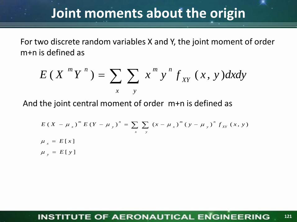
Joint moments about the origin
For two continuous random variables X and Y, the joint moment of order m+n is defined as
dxdyyxfyxYXEXY
nmnm
),()(
And the joint central moment of order m+n is defined as
][
][
),()()()()(
yE
xE
dxdyyxfyxYEXE
y
x
XY
n
y
m
x
n
y
m
x
117

Covariance of two random variables
The covariance of two random variables X and Y is defined as
Cov(X, Y) is also denoted as ςXY.
Cov(X,Y)=E(X-μx)E(Y- μy)
yx
YXXY
yxxy
n
y
m
x
XYE
yEXEXYE
YXXYE
YEXEYXCov
)(
)()()(
)(
)()(),(
118

Uncorrelated random variables
Two random variables are called uncorrelated if
Cov(X,Y)=0
Which also means E(XY)=μxμy
If are independent random variables, then
Thus two independent random variables are always uncorrelated.
)()(),( yfxfyxfYXXY
119

joint characteristic function
The joint characteristic function of two random variables X and Y is defined by
If and are jointly continuous random variables, then
dxdyeyxf
yjxj
XYYX
21),(),(21,
][),( 21
21
yjxj
XYeE
120
Joint moments about the origin
For two discrete random variables X and Y, the joint moment of order m+n is defined as
And the joint central moment of order m+n is defined as
dxdyyxfyxYXE
x y
XY
nmnm
),()(
][
][
),()()()()(
yE
xE
yxfyxYEXE
y
x
XY
n
y
m
x
x y
n
y
m
x
121

Covariance of two random variables
The covariance of two random variables X and Y is defined as
Cov(X, Y) is also denoted as ςXY.
Cov(X,Y)=E(X-μx)E(Y- μy)
yx
YXXY
yxxy
n
y
m
x
XYE
yEXEXYE
YXXYE
YEXEYXCov
)(
)()()(
)(
)()(),(
122
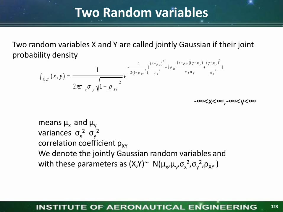
Two Random variables
Two random variables X and Y are called jointly Gaussian if their joint probability density
])())((
2)(
[
)1(2
1
2,
2
2
2
2
2
12
1),( Y
y
YX
yX
XY
X
x
XY
yyxx
XYyx
YXeyxf
-∞<x<∞,-∞<y<∞
means μx and μy
variances ςx2 ςy
2
correlation coefficient ρXY
We denote the jointly Gaussian random variables and with these parameters as (X,Y)~ N(μx,μy,ςx
2,ςy2,ρXY )
123

Transformations of multiple random variables
The joint density function of new random variable Yi=T(X1,X2,……XN) i=1,2,3….n
The random variable Xj can be obtained from inverse transformationX j=Tj
-1(Y1,Y2,…..YN)
**
y,,y,ygx
y,,y,ygx
y,,y,ygx
nknn
k
k
211
211
22
211
11
124

• Assuming that the partial derivatives exist at every point (y1, y2,…,yk=n). Under these assumptions, we have the following determinant J
called as the Jacobian of the transformation specified by (**). Then, the joint pdf of Y1, Y2,…,Yk can be obtained by using the change of variable technique of multiple variables.
ii y/g 1
Transformations of multiple random variables
n
nn
n
y
g
y
g
y
g
y
g
detJ1
1
1
11
1
11
125

• As a result, the new p.d.f. is defined as follows:
otherwise
yyyJgggfyyyg
nnXX
n
n
,0
,,,for |,|,,,,,,
21
11
2
1
1,,
21
1
Transformations of multiple random variables
126
Linearly transformation of Gaussian RV
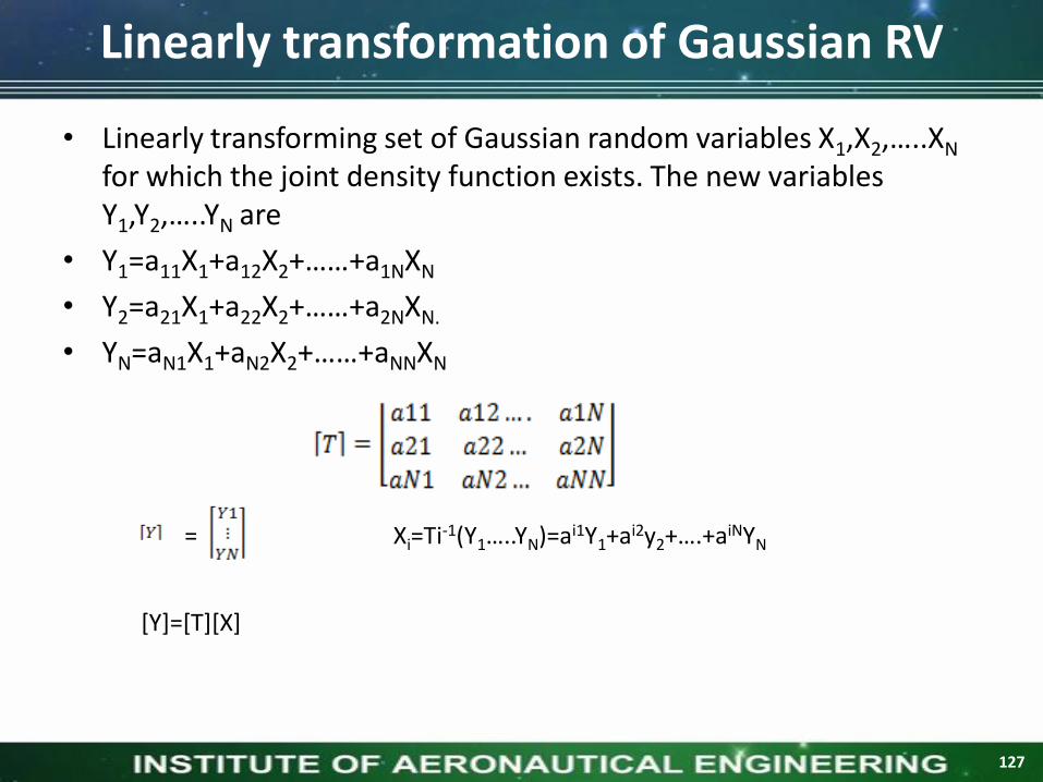
• Linearly transforming set of Gaussian random variables X1,X2,…..XN
for which the joint density function exists. The new variables Y1,Y2,…..YN are
• Y1=a11X1+a12X2+……+a1NXN
• Y2=a21X1+a22X2+……+a2NXN.
• YN=aN1X1+aN2X2+……+aNNXN
=
[Y]=[T][X]
Xi=Ti-1(Y1…..YN)=ai1Y1+ai2y2+….+aiNYN
127

UNIT-IVStochastic Processes: Temporal
Characteristics
128

Random Process
The concept of random variable was defined previously as mapping from the Sample Space S to the real line as shown below
Sample Space
S
2ns 1ns
ns
1ns
1nx
2nx
nx
1nx
A random process is a process (i.e.,variation in time or one dimensionalspace) whose behavior is notcompletely predictable and can becharacterized by statistical laws.
Examples of random processesDaily stream flowHourly rainfall of storm eventsStock index
129

The concept of randomprocess can be extended toinclude time and the outcomewill be random functions oftime as shown besideWhere s is the outcome ofan experiment
The functions
are one realizations of many ofthe random process X(t)
2 1 1( ), ( ), ( ), ( ),
n n n nx t x t x t x t
A random process also represents a random variable when time is fixed
1X (t ) is a random variable
Random Process (Contd..)
),( stx
130

Classification of Random Process
Classification of random process
Continuous random process
Discrete random process
Continuous random sequence
Discrete random sequence
Continuous time t => x(t) = Random processDiscrete time n => x[n] = Random sequence
131
Continuous Random Process
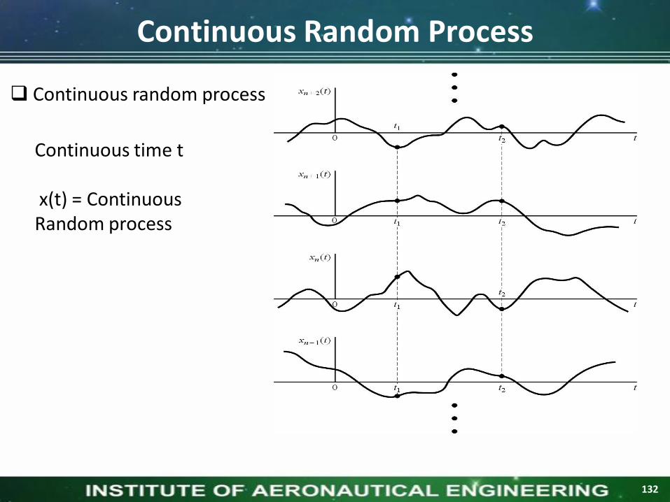
Continuous random process
Continuous time t
x(t) = Continuous Random process
132

Discrete Random Process
Discrete random process
Continuous time t
x(t) = Discrete Random process
133
Continuous Random Sequence
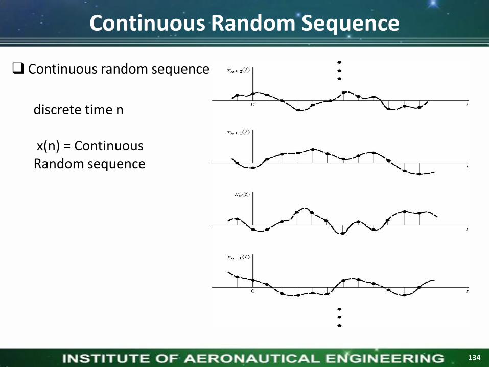
Continuous random sequence
discrete time n
x(n) = Continuous Random sequence
134
Discrete Random Sequence
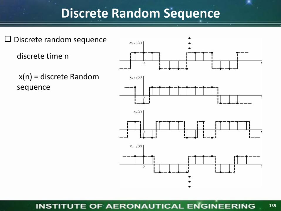
Discrete random sequence
discrete time n
x(n) = discrete Random sequence
135
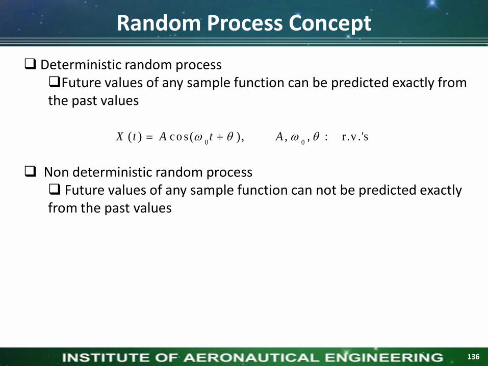
Random Process Concept
0( ) co s ( ),X t A t
0, , : r .v .'sA
Deterministic random processFuture values of any sample function can be predicted exactly from the past values
Non deterministic random process Future values of any sample function can not be predicted exactly from the past values
136
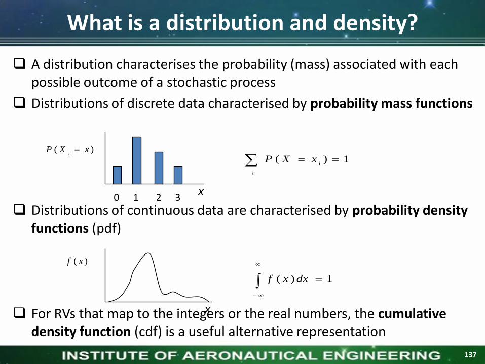
What is a distribution and density?
A distribution characterises the probability (mass) associated with each possible outcome of a stochastic process
Distributions of discrete data characterised by probability mass functions
Distributions of continuous data are characterised by probability density functions (pdf)
For RVs that map to the integers or the real numbers, the cumulative density function (cdf) is a useful alternative representation
1)( i
ixXP
1)(
dxxf
)( xXPi
x
)( xf
x
0 1 2 3
137

Stationary and Independence
Stationary Random Process all its statistical properties do not change with time
Non Stationary Random Process not stationary
138

First-order densities of a random process
A stochastic process is defined to be completely or totallycharacterized if the joint densities for the random variables
are known for all times and all n.)(),(),(21 n
tXtXtX nttt ,,,
21
Stationary and Independence (Contd..)
For a specific t, X(t) is a random variable with distribution
The function F(x,t) is defined as the first-order distribution of the random variable X(t). Its derivative with respect to x
is the first-order density of X(t).
])([),( xtXptxF
x
txFtxf
),(),(
139

If the first-order densities defined for all time t, i.e. f(x,t), are all thesame, then f(x,t) does not depend on t and we call the resultingdensity the first-order density of the random process {x(t)} ; otherwise,we have a family of first-order densities.
The first-order densities (or distributions) are only a partialcharacterization of the random process as they do not containinformation that specifies the joint densities of the random variablesdefined at two or more different times.
Stationary and Independence (Contd..)
140
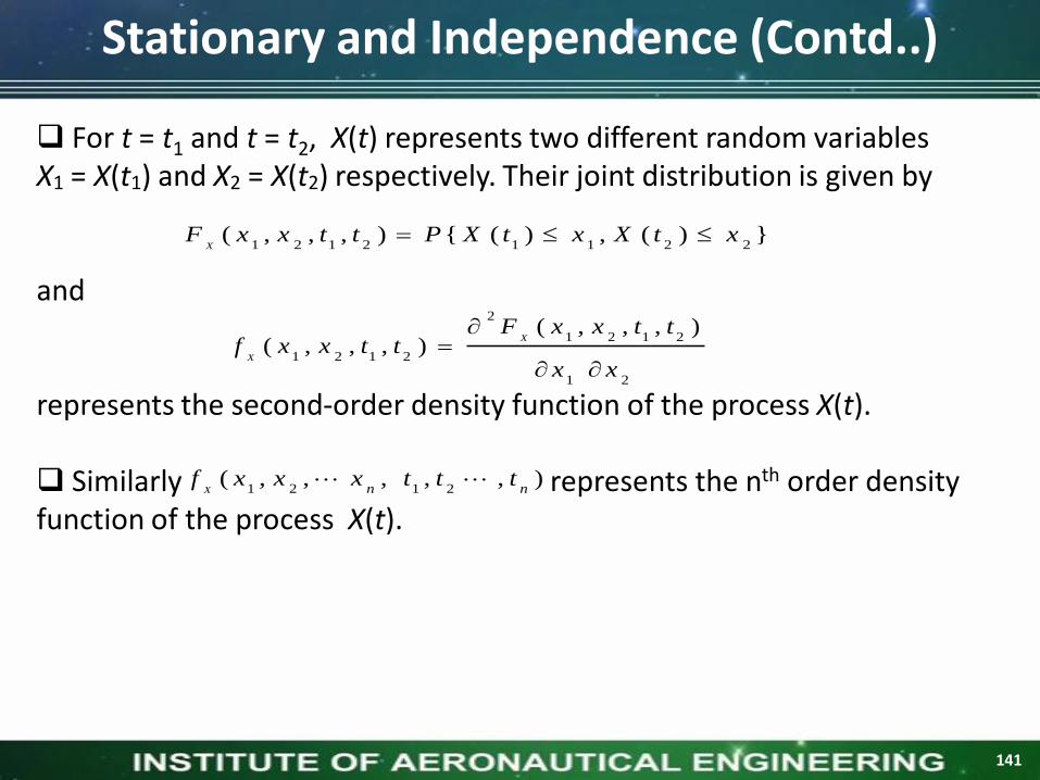
For t = t1 and t = t2, X(t) represents two different random variablesX1 = X(t1) and X2 = X(t2) respectively. Their joint distribution is given by
and
represents the second-order density function of the process X(t).
Similarly represents the nth order densityfunction of the process X(t).
})(,)({),,,(22112121
xtXxtXPttxxFX
2
1 2 1 2
1 2 1 2
1 2
( , , , )( , , , )
X
X
F x x t tf x x t t
x x
),, ,,,(2121 nn
tttxxxfX
Stationary and Independence (Contd..)
141

Mean and variance of a random process
The first-order density of a random process, f(x,t), gives theprobability density of the random variables X(t) defined for all time t.The mean of a random process, mX(t), is thus a function of time specifiedby
ttttX
dxtxfxXEtXEtm ),(][)]([)(
For the case where the mean of X(t) does not depend on t, we have
The variance of a random process, also a function of time, is defined by
constant) (a )]([)(XX
mtXEtm
2222)]([][)]()([)( tmXEtmtXEt
XtXX
142
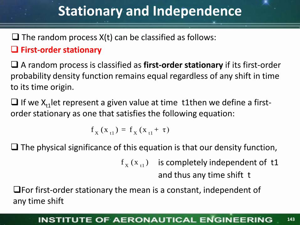
The random process X(t) can be classified as follows:
Stationary and Independence
First-order stationary
A random process is classified as first-order stationary if its first-orderprobability density function remains equal regardless of any shift in time to its time origin.
If we Xt1let represent a given value at time t1then we define a first-order stationary as one that satisfies the following equation:
X t1 X t1f (x ) = f (x + τ )
The physical significance of this equation is that our density function,
X t1f (x ) is completely independent of t1
and thus any time shift t
For first-order stationary the mean is a constant, independent of any time shift
143

Second-order stationary
A random process is classified as second-order stationary if its second-order probability density function does not vary over any time shiftapplied to both values.
In other words, for values Xt1 and Xt2 then we will have the followingbe equal for an arbitrary time shift t
X t1 t2 X t1 + τ t2 + τf (x ,x ) = f (x ,x )
From this equation we see that the absolute time does not affect ourfunctions, rather it only really depends on the time difference betweenthe two variables.
Stationary and Independence (Contd..)
144

For a second-order stationary process, we need to look at theautocorrelation function ( will be presented later) to see its mostimportant property.
Since we have already stated that a second-order stationaryprocess depends only on the time difference, then all of these typesof processes have the following property:
X X
X X
R (t,t+ τ ) = E [X (t)X (t+ τ )]
= R (τ )
Stationary and Independence (Contd..)
145

Wide-Sense Stationary (WSS)
A process that satisfies the following:
E X (t) = X = co n s tan t
X XE X (t)X (t + τ ) = R (τ )
is a Wide-Sense Stationary (WSS)
Second-order stationary Wide-Sense Stationary
The converse is not true in general
The mean is a constant and the autocorrelation function depends only on the difference between the time indices
146

Similarly
,0}{sinsin}{coscos
)}{cos()}({)(
0
0
0
EtaEta
taEtXEtX
).(cos2
)}2)(cos()({cos2
)}cos(){cos(),(
210
2
210210
2
2010
2
21
tta
ttttEa
ttEattRXX
).2,0(~ ),cos()(0
UtatX
This gives
2
0 }.{sin0cos}{cos since
2
1 EdE
Wide-Sense Stationary (Example)
So given X(t) is WSS
Constant
147

Nth order and Strict-Sense Stationary
In strict terms, the statistical properties are governed by the jointprobability density function. Hence a process is nth-order Strict-SenseStationary (S.S.S) if
For any c, where the left side represents the joint density function ofthe random variablesand the right side corresponds to the joint density function of the randomvariables
A process X(t) is said to be strict-sense stationary if equation (1)true for all
)1(),, ,,,(),, ,,,(21212121
ctctctxxxftttxxxfnnnn XX
)( , ),( ),(2211 nn
tXXtXXtXX
).( , ),( ),(2211
ctXXctXXctXXnn
. and ,2 ,1 , , ,2 ,1 , canynniti
148

A stationary random process for which time averages equal ensembleaverages is called an ergodic process:
Ergodic Process
x
mnx
mnxmnxxx
149

1
0
1
0
22
1
0
1
1
1
L
nL
L
n
xx
L
n
x
nxmnxL
nxmnx
mnxL
nxL
m
ˆ
ˆ
In practice, we cannotcompute with the limits, butinstead the quantities.
Similar quantities are oftencomputed as estimates ofthe mean, variance, andautocorrelation.
Ergodic Process (Contd..)
It is common to assume that a given sequence is a sample sequence ofan ergodic random process, so that averages can be computed from asingle sequence.
150

Time Average and Ergodicity
The time average of a quantity is defined as
Here A is used to denote time average in a manner analogous to Efor the statistical average.
The time average is taken over all time because, as applied to randomprocesses, sample functions of processes are presumed to exist for alltime.
1[ ] lim [ ]
2
T
TT
A d tT
151

Let x(t) be a sample of the random process X(t) were the lower case letter imply a sample function.
We define the mean value x = A x (t)
( a lowercase letter is used to imply a sample function) and the time autocorrelation function
X X(τ ) as follows:
T
TT
1x = A x (t) = lim x (t) d t
2 T
X X(τ ) = A x (t)x (t + τ )
T
TT
1= lim x (t)x (t + τ ) d t
2 T
For any one sample function ( i.e., x(t) ) of the random process X(t), the last two integrals simply produce two numbers.
x A number for the averageX X
(τ )
for a specific value of
and a number for
Time Average and Ergodicity (Contd..)
152

Since the sample function x(t) is one out of other samples functions of the random process X(t),
The average xX X
(τ )and the autocorrelation are random variables
By taking the expected value for xX X
(τ )and ,we obtainT
TT
1E [x ] = E [A [x (t)]] = E lim x (t) d t
2 T
T
TT
1lim E [x (t)] d t
2 T
T
TT
1lim X d t
2 T
T
= lim X (1 )
= X
T
X XTT
1E [ (τ )] = E [A [x (t)x (t + τ )] ] = E lim x (t )x (t + τ ) d t
2 T
T T
X X X XT TT T
1 1= lim E [x (t)x (t + τ )] d t = lim R (τ ) d t = R (τ )
2 T 2 T
Time Average and Ergodicity (Contd..)
153

1( ) [ ( ) ( ) ] lim ( ) ( )
2
T
x yTT
A x t y t x t y t d tT
( ) ( )x x X X
x X
R
Time Average and Ergodicity (Contd..)
Time cross correlation
Ergodic =>
Jointly Ergodic => Ergodic X(t) and Y(t)
)()( XYxy
R
154

Introduction to Autocorrelation
Autocorrelation occurs in time-series studies when the errorsassociated with a given time period carry over into future time periods.
For example, if we are predicting the growth of stock dividends, anoverestimate in one year is likely to lead to overestimates insucceeding years.
Times series data follow a natural ordering over time.
It is likely that such data exhibit intercorrelation, especially if the timeinterval between successive observations is short, such as weeks ordays.
155

We expect stock market prices to move or move down for several daysin succession.
We experience autocorrelation when
Tintner defines autocorrelation as ‘lag correlation of a given serieswithin itself, lagged by a number of times units’ whereas serialcorrelation is the ‘lag correlation between two different series’.
Introduction (contd..)
0)( ji
uuE
156
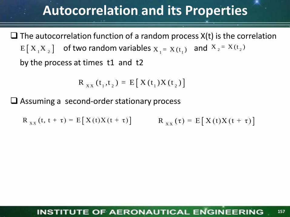
The autocorrelation function of a random process X(t) is the correlation
1 2E X X of two random variables
1 1X = X (t ) 2 2
X = X (t )and
by the process at times t1 and t2
X X 1 2 1 2R (t ,t ) = E X (t )X (t )
Assuming a second-order stationary process
X XR (t, t + τ ) = E X (t)X (t + τ ) X X
R (τ ) = E X (t)X (t + τ )
Autocorrelation and its Properties
157

Autocorrelation :
The value of x() at equal to 0 is the variance, x2
T
0Tx
dt x-τ)x(t.x-x(t)T
1Lim)(
The autocorrelation, or auto covariance, describes the general dependency of x(t) with its value at a short time later, x(t+)
time, t
x(t)
T
Normalized auto-correlation : R()= R(0)= 1
Autocorrelation and its Properties (Contd..)
x()/x2
158

The autocorrelation for a random process eventually decays tozero at large
R()
Time lag,
1
0
The autocorrelation for a sinusoidal process (deterministic) is acosine function which does not decay to zero
Autocorrelation and its Properties (Contd..)
159
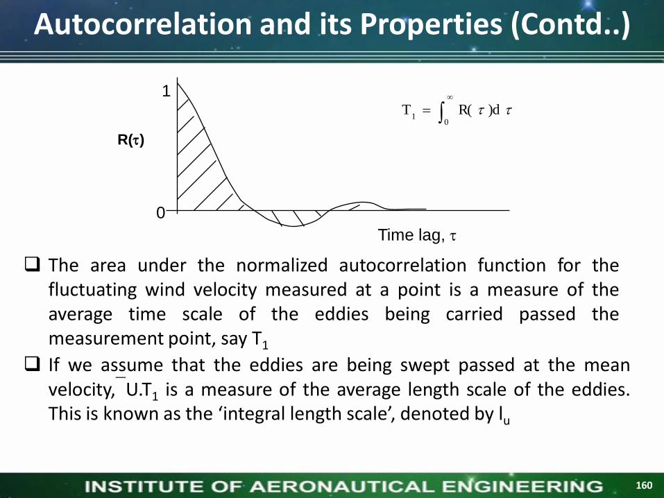
The area under the normalized autocorrelation function for thefluctuating wind velocity measured at a point is a measure of theaverage time scale of the eddies being carried passed themeasurement point, say T1
R()
Time lag,
1
0
If we assume that the eddies are being swept passed at the meanvelocity,U.T1 is a measure of the average length scale of the eddies.This is known as the ‘integral length scale’, denoted by lu
0
1)dR(T
Autocorrelation and its Properties (Contd..)
160

( , ) [ ( ) ( )] ( )X X X X
R t t E X t X t R
2
(1) ( ) (0 )
( 2 ) ( ) ( )
(3 ) (0 ) [ ( ) ]
X X X X
X X X X
X X
R R
R R
R E X t
( 4 ) s ta t io n a ry & e rg o d ic ( ) w ith n o p e r io d ic c o m p o n e n tsX t
2
| |
lim ( )X X
R X
(5 ) s ta t io n a ry ( ) h a s a p e r io d ic c o m p o n e n tX t
( ) h as a p e rio d ic co m p o n en t w ith th e sam e p e rio d .X X
R
Autocorrelation and its Properties (Contd..)
Properties of Autocorrelation function
161

Cross-correlation
T
0Txy
dt y-τ)y(t.x-x(t)T
1Lim)(c
The cross-correlation function describes the general dependency of x(t) with another random process y(t+), delayed by a time delay,
time, t
x(t)
T
time, t
y(t)
T
x
y
Cross-correlation
162
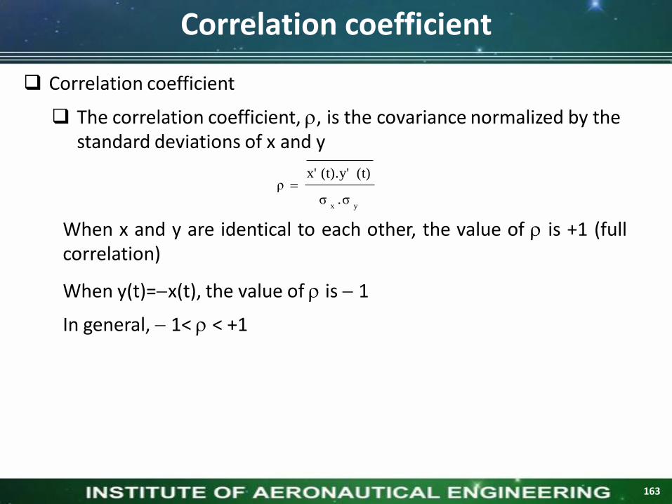
Correlation coefficient
The correlation coefficient, , is the covariance normalized by the standard deviations of x and y
When x and y are identical to each other, the value of is +1 (fullcorrelation)
When y(t)=x(t), the value of is 1
In general, 1< < +1
yx.σσ
(t)(t).y'x'ρ
Correlation coefficient
163

Correlation - application :
The fluctuating wind loading of a tower depends on the correlation coefficient between wind velocities and hence wind loads, at various heights
For heights, z1, and z2
: )(z). σ(zσ
)(z).u'(zu')z,ρ(z
2u1u
21
21
z1
z2
Application of correlation
164

Properties of Cross Correlation
( ) [ ( ) ( )]X Y
R E X t Y t
(1) ( ) ( )
( 2 ) ( ) (0 ) (0 )
1(3 ) ( ) (0 ) (0 )
2
X Y Y X
X Y X X Y Y
X Y X X Y Y
R R
R R R
R R R
2[{ ( ) ( )} ] 0 ,E Y t X t
1( 0 ) ( 0 ) [ ( 0 ) ( 0 )]
2X X Y Y X X Y Y
R R R R
Properties of cross-correlation function of jointly w.s.s. r.p.’s:
165

Example of Cross Correlation
0, : r .v .'s co n s tA B
2 2 2[ ] [ ] 0 , [ ] 0 , [ ] [ ]E A E B E A B E A E B
0 0 0 0( ) co s ( ) s in ( ), ( ) co s ( ) s in ( )X t A t B t Y t B t A t
0 0 0 0[ ( )] [ co s ( ) s in ( )] [ ] co s ( ) [ ] s in ( ) 0E X t E A t B t E A t E B t
2
0 0 0 0 0 0
2
0 0 0 0 0 0
2 2
0 0 0 0 0 0 0
( , ) [ ( ) ( ) ]
[ c o s ( ) c o s ( ) c o s ( ) s in ( )
s in ( ) c o s ( ) s in ( ) s in ( ) ]
{ c o s ( ) c o s ( ) s in ( ) s in ( )} c o s ( )
X XR t t E X t X t
E A t t A B t t
A B t t B t t
t t t t
( ) : w .s .s .X t
166
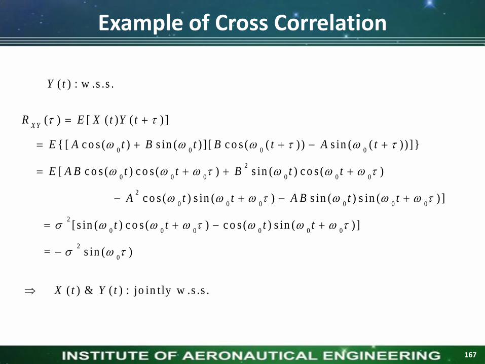
( ) : w .s .s .Y t
0 0 0 0
2
0 0 0 0 0 0
2
0 0 0 0 0 0
( ) [ ( ) ( ) ]
{ [ c o s ( ) s in ( ) ] [ c o s ( ( ) ) s in ( ( ) ) ]}
[ c o s ( ) c o s ( ) s in ( ) c o s ( )
c o s ( ) s in ( ) s in ( ) s in ( ) ]
X YR E X t Y t
E A t B t B t A t
E A B t t B t t
A t t A B t t
2
0 0 0 0 0 0
2
0
[ s in ( ) c o s ( ) c o s ( ) s in ( ) ]
= s in ( )
t t t t
( ) & ( ) : jo in t ly w .s .s .X t Y t
Example of Cross Correlation
167

Covariance
T
0Txy
dt y-y(t).x-x(t)T
1Lim(t)y(t).x(0)c
The covariance is the cross correlation function with the time delay, , set to zero
Note that here x'(t) and y'(t) are used to denote the fluctuating parts of x(t) and y(t) (mean parts subtracted)
Covariance
168

Auto Covariance
The auto covariance Cx(t1,t2) of a random process X(t) is defined as the covariance of X(t1) and X(t2)
Cx(t1,t2)=E[{X(t1)-mx(t1)}{X(t2)-mx(t2)}]
Cx(t1,t2) = Rx(t1,t2)-mx(t1)mx(t2)
The variance of X(t) can be obtained from Cx(t1,t2)
VAR[X(t)] = E[(X(t)-mx(t))2] = Cx(t,t)
The correlation coefficient of X(t) is given by
1)t,(tρ
),(),(
),()t,(tρ
21x
2211
21
21x
ttCttC
ttC
XX
X
169
Auto Covariance Example#1
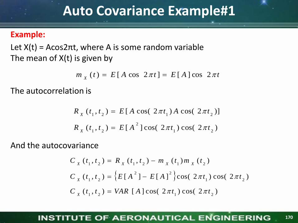
Example:
Let X(t) = Acos2πt, where A is some random variableThe mean of X(t) is given by
The autocorrelation is
And the autocovariance
tAEtAEtmX
2cos][]2cos[)(
)2cos()2cos(][),(
)]2cos()2cos([),(
21
2
21
2121
ttAEttR
tAtAEttR
X
X
)2cos()2cos(][),(
)2cos()2cos(][][),(
)()(),(),(
2121
21
22
21
212121
ttAVARttC
ttAEAEttC
tmtmttRttC
X
X
XXXX
170

Auto Covariance Example#2
Let X(t) = cos(ωt+θ), where θ is uniformly distributed in the interval (-π, π).The mean of X(t) is given by
The autocorrelation and autocovariance are then
0)cos(2
1)][cos()(
ttEtmX
))(cos(2
1),(
)2)(cos())(cos(2
1
2
1),(
)]cos()[cos(),(),(
2121
212121
212121
ttttC
dttttttC
ttEttRttC
X
X
XX
Example:
171
Cross Covariance
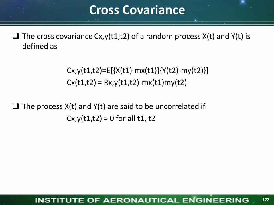
The cross covariance Cx,y(t1,t2) of a random process X(t) and Y(t) is defined as
Cx,y(t1,t2)=E[{X(t1)-mx(t1)}{Y(t2)-my(t2)}]
Cx(t1,t2) = Rx,y(t1,t2)-mx(t1)my(t2)
The process X(t) and Y(t) are said to be uncorrelated if
Cx,y(t1,t2) = 0 for all t1, t2
172

Random sequence
R a n d o m S e q u e n c e (= D is c re te -t im e R .P )
( ) [ ]s
X n T X n
M e a n ( [ ] )E X n
( , ) ( [ ] [ ])X X
R n n k E X n X n k
( , ) { ( [ ] [ ])( [ ] [ ] )}
( , ) [ ] [ ]
X X
X X
C n n k E X n X n X n k X n k
R n n k X n X n k
( , ) ( [ ] [ ])X Y
R n n k E X n Y n k
( , ) { ( [ ] [ ])( [ ] [ ])}
( , ) [ ] [ ]
X Y
X Y
C n n k E X n X n Y n k Y n k
R n n k X n Y n k
173

Let X(t) be a random process and let X(t1), X(t2), ….X(tn) be the randomvariables obtained from X(t) at t=t1,t2……..tn sec respectively
Let all these random variables be expressed in the form of a matrix
Then, X(t) is referred to as normal or Gaussian process if all theelements of X are jointly Gaussian
Gaussian Random Process
)(
)(
)(
2
1
ntX
tX
tX
X
174

Gaussian Random Process
( ) ,X t t - c o n t in u o u s r .p .
1
1 1
1 1( , , ; , , ) e x p { [ ] [ ]}
2( 2 )
t
X N N XN
X
f x x t t x X C x X
C
[ ( )]i i
X E X t ( , )ik X X i k
C C t t
s ta tio n a ry [ ( )] (c o n s t) & ( , ) ( )X X i k X X k i
E X t X R t t R t t
( , ) ( )X X i k X X k i
C t t C t t
w .s .s . G a u s s ia n s t r ic t ly s ta t io n a ry
175
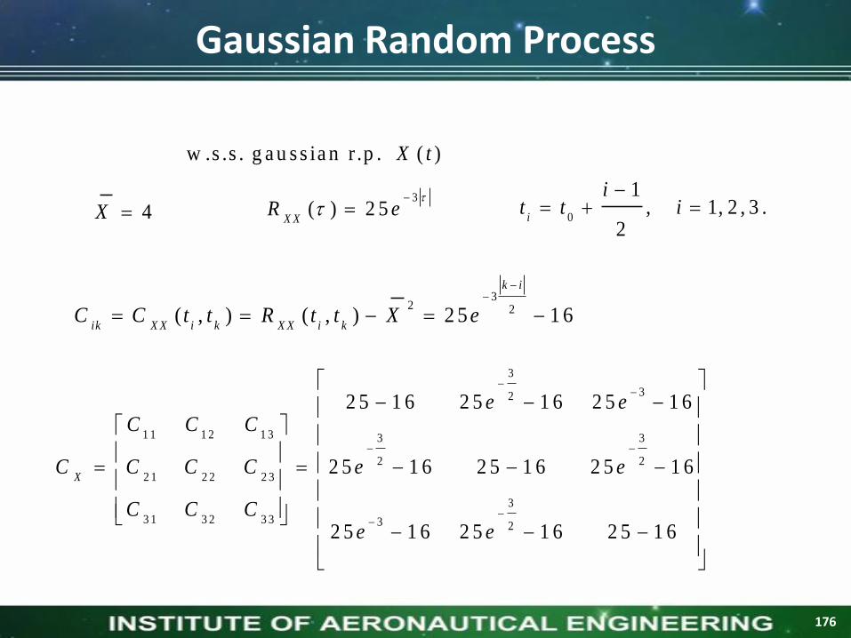
w .s .s . g a u s s ia n r .p . ( )X t
4X 3
( ) 2 5X X
R e
0
1, 1, 2 , 3 .
2i
it t i
32 2( , ) ( , ) 2 5 1 6
k i
ik X X i k X X i kC C t t R t t X e
3
32
1 1 1 2 1 3 3 3
2 2
2 1 2 2 2 3
3
3 1 3 2 3 3 3 2
2 5 1 6 2 5 1 6 2 5 1 6
2 5 1 6 2 5 1 6 2 5 1 6
2 5 1 6 2 5 1 6 2 5 1 6
X
e eC C C
C C C C e e
C C Ce e
Gaussian Random Process
176

Properties of Gaussian Process
If a gaussian process X(t) is applied to a stable linear filter, then therandom process Y(t) developed at the output of the filter is alsogaussian.
Considering the set of random variables or samples X(t1),X(t2),…..X(tn) obtained by observation of a random process X(t) atinstants t1,t2,…….tn, if the process X(t) is gaussian, then this set ofrandom variables are jointly gaussian for any n, with their n-fold jointp.d.f. being completely determined by the set of means.
mx(ti) = E[X(ti)] for i=1,2,….n
and the set of auto covariance function
Cxx(t1,t2) = E[{X(t1)-E[X(t1)]}{X(t2)-E[X(t2)]}]
If a gaussian process is wide sense stationary, then the process is alsostationary in the strict sense
If the set of random variables X(t1),X(t2)…X(tn) are uncorrelated thenthey are statistically independent
177

Poisson Random Process
we introduced Poisson arrivals as the limiting behaviorof Binomial random variables
where
,2 ,1 ,0 ,!" duration of interval
an inoccur arrivals "
k
ke
kP
k
T
Tnp
0 T
arrivals k
20 T
arrivals k
178
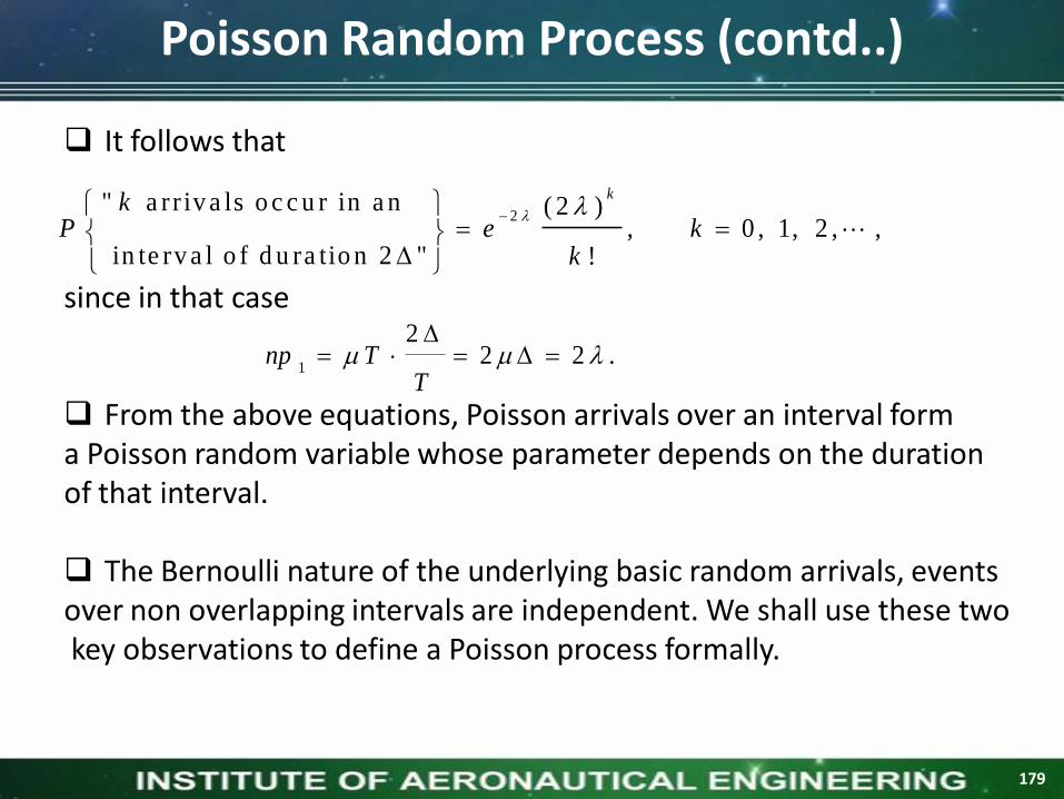
It follows that
since in that case
From the above equations, Poisson arrivals over an interval forma Poisson random variable whose parameter depends on the durationof that interval.
The Bernoulli nature of the underlying basic random arrivals, eventsover non overlapping intervals are independent. We shall use these twokey observations to define a Poisson process formally.
.222
1
TTnp
2" a r r iv a ls o c c u r in a n ( 2 )
, 0 , 1, 2 , , in te rv a l o f d u ra tio n 2 " !
kkP e k
k
Poisson Random Process (contd..)
179

and(ii) If the intervals (t1, t2) and (t3, t4) are non overlapping, then the random variables n(t1, t2) and n(t3, t4) are independent. Since n(0, t) ~ we have
and
1221 ,,2 ,1 ,0 ,
!
)(}) ,({ tttk
k
tekttnP
k
t
),( tP
ttnEtXE )] ,0([)]([
.)] ,0([)]([2222
tttnEtXE
Definition: X(t) = n(0, t) represents a Poisson process if(i) the number of arrivals n(t1, t2) in an interval (t1, t2) of length t = t2 – t1
is a Poisson random variable with parameterThus
.t
Poisson Random Process (contd..)
180

But
and hence the left side of above equation can be rewritten as
Similarly
Thus
)()(),0() ,0() ,(121221
tXtXtntnttn
)].([) ,()}]()(){([1
2
21121tXEttRtXtXtXE
XX
. ,
)]([) () ,(
1221
2
1
1
2
121
2
21
ttttt
tXEtttttRXX
. , ) ,(1221
2
221tttttttR
XX
). , min( ) ,(2121
2
21ttttttR
XX
To determine the autocorrelation function let t2 > t1 , then from (ii) above n(0, t1) and n(t1, t2) are independent Poisson random variables with parameters and respectively. Thus
), ,(21
ttRXX
1t )(
12tt
).()] ,([)] ,0([)] ,() ,0([121
2
211211tttttnEtnEttntnE
Poisson Random Process (contd..)
181

Notice that the Poisson process X(t) does not represent a wide sense stationary process.
Define a binary level process
that represents a telegraph signal Notice that the transitioninstants {ti} are random Although X(t) does not represent awide sense stationary process,
)()1()(
tXtY
01
ti
t
t
)( tX
t
)( tY
t
1
Poissonarrivals
1
1t
Poisson Random Process (contd..)
182
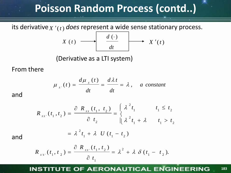
its derivative does represent a wide sense stationary process.
From there
and
and
)( tX
)( tX )( tX dt
d )(
(Derivative as a LTI system)
2
1 1 21 2
1 2 2
2 1 1 2
2
1 1 2
( , )( )
( )
X X
X X
t t tR t tR t , t
t t t t
t U t t
constant adt
td
dt
tdt
X
X ,
)()(
).(
) ,( )(
21
2
1
21
21 tt
t
ttR, ttR
XX
XX
Poisson Random Process (contd..)
183
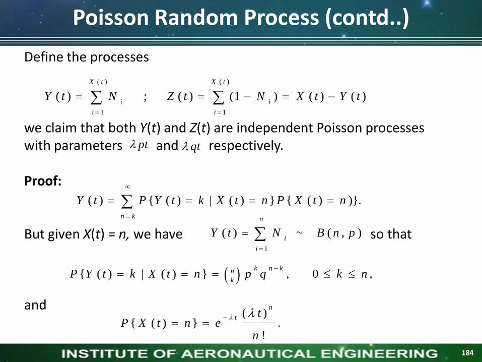
Define the processes
we claim that both Y(t) and Z(t) are independent Poisson processeswith parameters and respectively.
Proof:
But given X(t) = n, we have so that
and
pt qt
kn
ntXPntXktYPtY )}.)({})(|)({)(
)()()1()( ; )(
)(
1
)(
1
tYtXNtZNtY
tX
i
i
tX
i
i
),( ~ )(
1
pnBNtY
n
i
i
{ ( ) | ( ) } , 0 ,k n kn
kP Y t k X t n p q k n
( ){ ( ) } .
!
n
t tP X t n e
n
Poisson Random Process (contd..)
184

More generally,
( ) ( )!
( ) ! ! ! ( ) !
(1 )
{ ( ) } ( )!
( ) ( ) , 0 , 1 , 2 ,
! !
~ ( ) .
n n k
q t
k t
t q tt k n k kn
n k k n n k
n k n k
e
q t k
k p t
p eP Y t k e p q t
k
e p tp t e k
k k
P p t
( ( ) ) ( (
{ ( ) , ( ) } { ( ) , ( ) ( ) }
{ ( ) , ( ) }
{ ( ) | ( ) } { ( ) }
( ) ( ) ( )
( ) ! ! !
k m n n
k m t p t q tk m
k
P Y t k P Z
P Y t k Z t m P Y t k X t Y t m
P Y t k X t k m
P Y t k X t k m P X t k m
t p t q tp q e e e
k m k m
) )
{ ( ) } { ( ) } ,
t m
P Y t k P Z t m
which completes the proof.
Poisson Random Process (contd..)
185

Poisson Random Process (contd..)
( ) ,X t t -- in te g e r-v a lu e d d is c re te r .p .
( 0 ) 0X ( ) ( )b a b a
t t X t X t
( )[ ( )][ ( ) ( ) ] , 0 ,1, 2 ,
!
a b
k
t ta b
a b
t tP X t X t k e k
k
( ) ( ) & ( ) ( ) a re in d ep .d c b a a b c d
t t t t X t X t X t X t
( ) [ ( )]X t E X t t 2 2
( , ) [ ( ) ] ( )X X
R t t E X t t t
( , )X X
C t t t
186
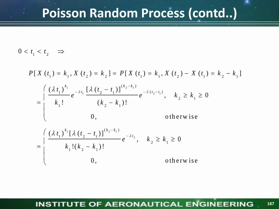
1 20 t t
1 2 1
1 2 1
1 2 1
2
1 1 2 2 1 1 2 1 2 1
( )
( )1 2 1
2 1
1 2 1
( )
1 2 1
2 1
1 2 1
[ ( ) , ( ) ] [ ( ) , ( ) ( ) ]
( ) [ ( ) ], 0
! ( ) !
0 , o th e rw is e
( ) [ ( ) ], 0
!( ) !
0 , o th e rw is e
k k k
t t t
k k k
t
P X t k X t k P X t k X t X t k k
t t te e k k
k k k
t t te k k
k k k
Poisson Random Process (contd..)
187

1 20 t t
2 1
2 1
2 2 1 1 2 1 2 1 1 1
2 1 2 1
( )
( )2 1
2 1
2 1
[ ( ) ( ) ] [ ( ) ( ) ( ) ]
[ ( ) ( ) ]
[ ( ) ],
( ) !
0 , o th e rw is e
k k
t t
P X t k X t k P X t X t k k X t k
P X t X t k k
t te k k
k k
Poisson Random Process (contd..)
188

( ) P o is s o n r .p .X t
1 2 30 t t t
1 2 30 k k k
3 21 2 1
1 2 1
1 1 2 2 3 3
1 1 2 1 2 1 3 2 3 2
1 1 2 1 2 1 3 2 3 2
( )( )
( ) 3 21 2 1
1 2 1 3
[ ( ) , ( ) , ( ) ]
[ ( ) , ( ) ( ) , ( ) ( ) ]
[ ( ) ] [ ( ) ( ) ] [ ( ) ( ) ]
[ ( ) ]( ) [ ( ) ]
! ( ) ! (
k kk k k
t t t
P X t k X t k X t k
P X t k X t X t k k X t X t k k
P X t k P X t X t k k P X t X t k k
t tt t te e
k k k k
3 2
3 21 2 1
3
( )
2
( )( )
1 2 1 3 2
1 2 1 3 2
) !
( ) [ ( ) ] [ ( ) ]
!( ) !( ) !
t t
k kk k k
t
ek
t t t t te
k k k k k
Example
189

UNIT-VStochastic Processes: Spectral
Characteristics
190
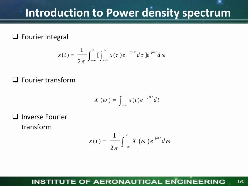
Introduction to Power density spectrum
Fourier integral
1( ) ( )
2
j tx t X e d
1( ) [ ( ) ]
2
j j tx t x e d e d
( ) ( )j t
X x t e d t
Fourier transform
Inverse Fourier
transform
191

22 2 1( ) ( ) ( ) ( )
2
T
T TT
E T x t d t x t d t X d
( ) ( ) ( )T
j t j t
T TT
X x t e d t x t e d t
( ) ,( )
0 , /T
x t T t Tx t
o w
A ssu m e ( ) , fo r a ll f in ite .T
TT
x t d t T
Introduction (Contd..)
Energy contained in x(t) in the interval (-T,T)
192

( ) ( ) , ta k e e x p e c ta t io n , le t .x t X t T
2{ [ ( ) ]}
X XP A E X t
p o w e r d e n s i ty s p e c tru m
2
2( )1 1
( ) ( )2 2 2
TT
T
XP T x t d t d
T T
2
2[ ( ) ]1 1
[ ( ) ]2 2 2
lim limT
T
X XT
T T
E XP E X t d t d
T T
1( )
2X X X X
P S d
2
[ ( ) ]
2lim
T
X X
T
E XS
T
Average power in x(t) in the interval (-T,T)
Introduction (Contd..)
Average power in random process x(t)
193

2 2
2 2 2 0 0
0 0 0
2 2 2 2
0 0 0 02 20 0 00
2 2
0 0
0
[ ( ) ] [ c o s ( )] [ c o s ( 2 2 )]2 2
2c o s ( 2 2 ) s in ( 2 2 )
2 2 2 2
s in ( 2 )2
A AE X t E A t E t
A A A At d t
A At
2 2 2
2 0 0 0
0
1{ [ ( ) ]} [ s in ( 2 )]
2 2 2lim
T
X XT
T
A A AP A E X t t d t
T
2{ [ ( ) ]}
X XP A E X t
w .s .s . (0 )X X X X
P R
0 0( ) co s ( )X t A t -- u n ifo rm ly d is tr ib u te d o n (0 , )
2
Example-1
Example-
1
194

p o w e r d e n s i ty s p e c tru m
0 0( ) co s ( )X t A t
0 0
0 0
0 0 0
( ) ( )0 0
0 0
0 0
0 0
1( ) c o s ( ) [ ]
2
2 2
s in [( ) ] s in [( ) ]
( ) ( )
T Tj t j tj t j j j t
TT T
T Tj t j tj j
T T
j j
X A t e d t A e e e e e d t
A Ae e d t e e d t
T TA T e A T e
T T
1 s in ( )2
j T j TT T
j t j t
t TT
e e Te d t e T
j j T
2
[ ( ) ]
2lim
T
X X
T
E XS
T
Example-
2
Example-2
195
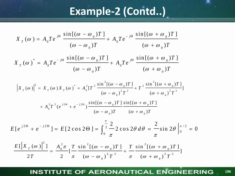
2 22 * 2 2 20 0
0 2 2 2 2
0 0
2 2 2 2 0 0
0
0 0
s in [( ) ] s in [( ) ]( ) ( ) ( ) [ ]
( ) ( )
s in [( ) ] s in [( ) ]( )
( ) ( )
T T T
j j
T TX X X A T T
T T
T TA T e e
T T
0 0
0 0
0 0
s in [( ) ] s in [( ) ]( )
( ) ( )
j j
T
T TX A T e A T e
T T
2 2 / 22
00
2 2[ ] [ 2 c o s 2 ] 2 c o s 2 s in 2 0
j jE e e E d
22 2 2
0 0 0
2 2 2 2
0 0
[ ( ) ] s in [( ) ] s in [( ) ][ ]
2 2 ( ) ( )
TE X A T TT T
T T T
* 0 0
0 0
0 0
s in [( ) ] s in [( ) ]( )
( ) ( )
j j
T
T TX A T e A T e
T T
Example-2 (Contd..)
196

22
0
0 0
[ ( ) ]( ) lim [ ( ) ( ) ]
2 2
T
X XT
E X AS
T
2
2
, i f 0s in ( )lim (b )
0 , if 0( )T
T T
T
2
2
s in ( )(a ) & (b ) lim ( )
( )T
T T
T
2 2
2 2
s in ( ) s in 11 (a )
( )
T T T xd d x
T x T
2 2
0 0
0 0
1 1( ) [ ( ) ( )]
2 2 2 2X X X X
A AP S d d
Example-2 (Contd..)
dxx
x
2
2sin
197

Properties Power density spectrum
P ro p e r t ie s o f th e p o w e r d e n s i ty s p e c tru m :
(1) ( ) 0X X
S
( 2 ) ( ) rea l ( ) ( )X X X X
X t S S
(3) ( ) is rea lX X
S
21( 4 ) ( ) { [ ( ) ]}
2X X
S d A E X t
( ) ( )T
j t
TT
X X t e d t
* *[ ( ) ( ) ] [ ( ) ( )]
( ) lim lim ( )2 2
T T T T
X X X XT T
E X X E X XS S
T T
P F o f (2 ) :
* *( ) ( ) ( ) ( )
T Tj t j t
T TT T
X X t e d t X t e d t X
2
[ ( ) ]( ) lim
2
T
X XT
E XS
T
198
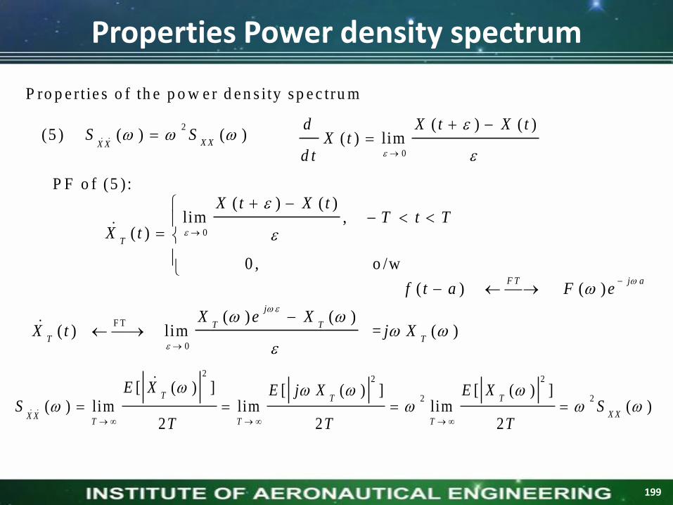
P ro p e r t ie s o f th e p o w e r d e n s i ty s p e c tru m
2(5 ) ( ) ( )
X XX XS S
22 2
2 2[ ( ) ] [ ( ) ] [ ( ) ]
( ) lim lim lim ( )2 2 2
T T T
X XX XT T T
E X E j X E XS S
T T T
P F o f (5 ) :
0
( ) ( )( ) lim
d X t X tX t
d t
0
( ) ( )lim ,
( )
0 , o /w
T
X t X tT t T
X t
F T
0
( ) ( )( ) lim = ( )
j
T T
T T
X e XX t j X
( ) ( )F T j a
f t a F e
Properties Power density spectrum
199

B a n d w id th o f th e p o w e r d e n s i ty s p e c tru m
( ) rea l ( ) evenX X
X t S
( ) lo w p ass fo rm X X
S
2
2
rm s
( )
( )
X X
X X
S d
W
S d
2
02 0
rm s
0
4 ( ) ( )
( )
X X
X X
S d
W
S d
ro o t m e a n s q u a re B a n d w id th
m e a n f re q u e n c y
rm s B W
( ) b an d p ass fo rm X X
S 0
0
0
( )
( )
X X
X X
S d
S d
Properties Power density spectrum
200
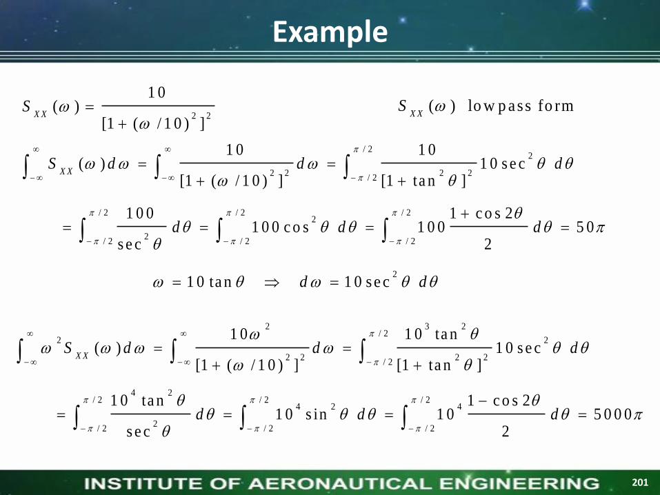
( ) lo w p ass fo rmX X
S 2 2
1 0( )
[1 ( / 1 0 ) ]X X
S
/ 22
2 2 2 2/ 2
/ 2 / 2 / 22
2/ 2 / 2 / 2
1 0 1 0( ) 1 0 s e c
[1 ( / 1 0 ) ] [1 ta n ]
1 0 0 1 c o s 21 0 0 c o s 1 0 0 5 0
s e c 2
X XS d d d
d d d
21 0 ta n 1 0 se cd d
2 3 2/ 2
2 2
2 2 2 2/ 2
4 2/ 2 / 2 / 2
4 2 4
2/ 2 / 2 / 2
1 0 1 0 ta n( ) 1 0 s e c
[1 ( / 1 0 ) ] [1 ta n ]
1 0 ta n 1 c o s 21 0 s in 1 0 5 0 0 0
s e c 2
X XS d d d
d d d
Example
201

2
2
rm s
( )
1 0 0
( )
X X
X X
S d
W
S d
rm s B W
2 2
1 0( )
[1 ( / 1 0 ) ]X X
S
rm s1 0 rad /secW
Example
202

Relationship between PSD and autocorrelation
1( ) [ ( , ) ]
2
( ) [ ( , ) ]
j
X X X X
j
X X X X
S e d A R t t
S A R t t e d
1 2
1 2
1 2
*
1 1 2 2
( )
1 2 2 1
( )
1 2 2 1
[ ( ) ( ) ] 1( ) lim lim [ ( ) ( ) ]
2 2
1lim [ ( ) ( ) ]
2
1lim ( , )
2
T Tj t j tT T
X XT TT T
T Tj t t
T TT
T Tj t t
X XT TT
E X XS E X t e d t X t e d t
T T
E X t X t e d t d tT
R t t e d t d tT
1 2
1 2
( )
1 2 2 1
( )
1 2 2 1
1 1 1( ) lim ( , )
2 2 2
1 1lim ( , )
2 2
T Tj t tj j
X X X XT TT
T Tj t t
X XT TT
S e d R t t e d t d t e dT
R t t e d d t d tT
203

( ) [ ( , )]j
X X X XS A R t t e d
1 2 1 2 2 1
1 1 1
1 1( ) lim ( , ) ( )
2 2
1 1lim ( , ) lim ( , )
2 2
[ ( , ) ]
T Tj
X X X XT TT
T T
X X X XT TT T
X X
S e d R t t t t d t d tT
R t t d t R t t d tT T
A R t t
( ) 1F T
t
( ) 1
1( )
2
j t
j t
t e d t
t e d
[ ( , ) ] ( )F T
X X X XA R t t S
Relationship between PSD and autocorrelation
204

( ) ( )j
X X X XS R e d
1( ) ( )
2
j
X X X XR S e d
( ) ( )F T
X X X XR S
( ) w .s .s . [ ( , )] ( )X X X X
X t A R t t R
Relationship between PSD and autocorrelation
205
Cross-power density spectrum
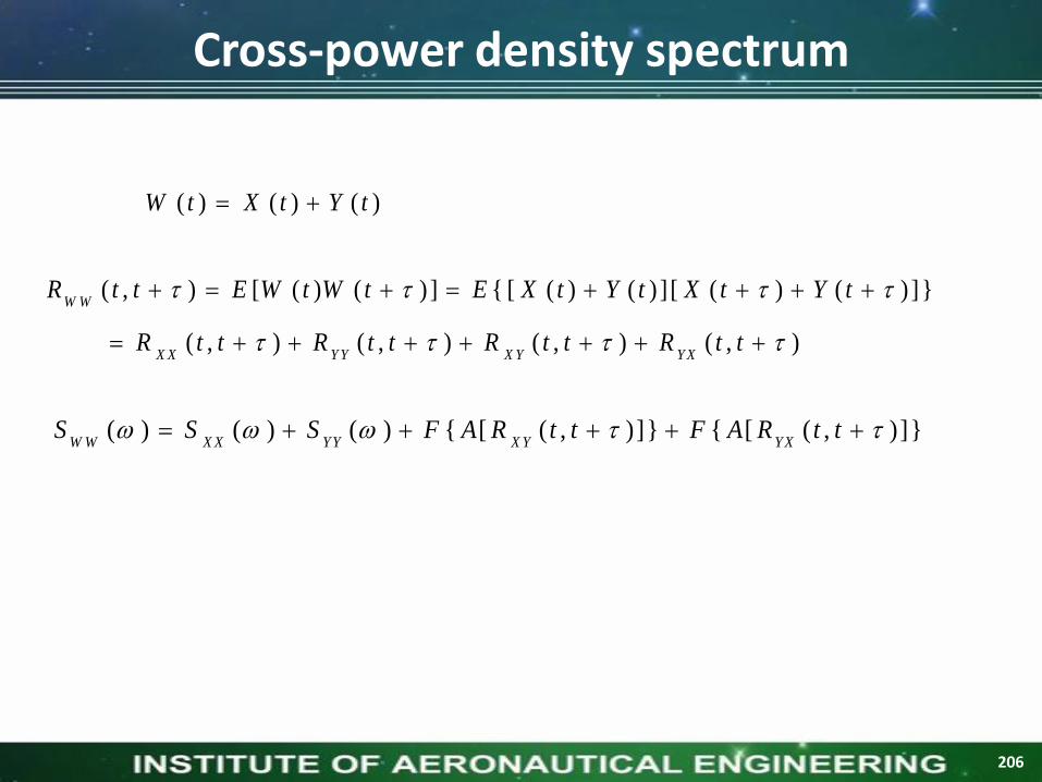
( ) ( ) ( )W t X t Y t
( , ) [ ( ) ( ) ] { [ ( ) ( ) ] [ ( ) ( ) ]}
( , ) ( , ) ( , ) ( , )
W W
X X Y Y X Y Y X
R t t E W t W t E X t Y t X t Y t
R t t R t t R t t R t t
( ) ( ) ( ) { [ ( , )]} { [ ( , )]}W W X X Y Y X Y YX
S S S F A R t t F A R t t
206

( ) ,( )
0 , /T
x t T t Tx t
o w
C ro s s P o w e r c o n ta in e d in ( ) , ( ) in th e in te rv a l ( , )x t y t T T
( ) ,( )
0 , /T
y t T t Ty t
o w
F T( ) ( )
T Tx t X
F T( ) ( )
T Ty t Y
P arseva l's th eo rem
A ssu m e ( ) & ( ) , fo r a ll f in ite .T T
T TT T
x t d t y t d t T
*( ) ( )1 1 1
( ) ( ) ( ) ( ) ( )2 2 2 2
TT T
X Y T TT
X YP T x t y t d t x t y t d t d
T T T
Cross-power density spectrum
207

a v e ra g e C ro s s P o w e r c o n ta in e d in ( ) , ( ) i n th e in te rv a l ( , )X t Y t T T
c ro s s -p o w e r d e n s i ty s p e c tru m
to ta l a v e ra g e C ro s s P o w e r c o n ta in e d in ( ) , ( )X t Y t
*[ ( ) ( )]1 1
lim ( , ) lim2 2 2
TT T
X Y X YTT T
E X YP R t t d t d
T T
*[ ( ) ( )]
( ) lim2
T T
X YT
E X YS
T
*[ ( ) ( )]1 1
( ) ( , )2 2 2
TT T
X Y X YT
E X YP T R t t d t d
T T
Cross-power density spectrum
208

T o ta l c ro ss p o w er = X Y YX
P P
( ) , ( ) o rth o g o n a l 0X Y Y X
X t Y t P P
1( )
2X Y X Y
P S d
*[ ( ) ( )]
( ) lim2
T T
Y XT
E Y XS
T
*1( )
2Y X Y X X Y
P S d P
Cross-power density spectrum
209

Properties of cross-power density spectrum
P ro p e r t ie s o f th e c ro s s -p o w e r d e n s i ty s p e c tru m :
*(1) ( ) ( ) ( )
X Y Y X Y XS S S
( ) ( )T
j t
TT
X X t e d t
* *[ ( ) ( )] [ ( ) ( ) ]
( ) lim lim ( )2 2
T T T T
Y X X YT T
E Y X E Y XS S
T T
P F o f (1 ) :
( ) , ( ) re a lX t Y t
* *
*[ ( ) ( )] [ ( ) ( ) ]( ) lim lim ( )
2 2
T T T T
Y X Y XT T
E Y X E Y XS S
T T
* *( ) ( ) ( ) ( )
T Tj t j t
T TT T
X X t e d t X t e d t X
210

( 2 ) R e[ ( )] & R e[ ( )] -- evenX Y YX
S S
( 4 ) ( ) & ( ) o rth o g o n a l ( ) ( ) 0X Y YX
X t Y t S S
(5 ) ( ) & ( ) u n c o rre la te d & h a v e c o n s t a n t m e a n ,
( ) ( ) 2 ( )X Y Y X
X t Y t X Y
S S X Y
(3) Im [ ( )] & Im [ ( )] -- o d dX Y Y X
S S
( ) & ( ) o rth o g o n a l ( , ) 0 A [ ( , )] 0X Y X Y
X t Y t R t t R t t
Properties of cross-power density spectrum
)(),(
)(),(
YX
FT
YX
XY
FT
XY
SttRA
SttRA
211

* ( ) 2 ( ) ( )
X Y Y XS X Y S
P F o f (5 ) : ( , ) [ ( , )]X Y X Y
R t t X Y A R t t X Y
( ) , ( ) -- jo in t ly w .s .s . X t Y t F T
( ) ( )X Y X Y
R S
F T( ) ( )
Y X Y XR S
Properties of cross-power density spectrum
212

Relationship between C-PSD and cross-correlation
1( ) [ ( , ) ]
2
( ) [ ( , ) ]
j
X Y X Y
j
X Y X Y
S e d A R t t
S A R t t e d
1 2
1 2
1 2
*
1 1 2 2
( )
1 2 2 1
( )
1 2 2 1
[ ( ) ( ) ] 1( ) lim lim [ ( ) ( ) ]
2 2
1lim [ ( ) ( ) ]
2
1lim ( , )
2
T Tj t j tT T
X YT TT T
T Tj t t
T TT
T Tj t t
X YT TT
E X YS E X t e d t Y t e d t
T T
E X t Y t e d t d tT
R t t e d t d tT
1 2
1 2
( )
1 2 2 1
( )
1 2 2 1
1 1 1( ) lim ( , )
2 2 2
1 1lim ( , )
2 2
T Tj t tj j
X Y X YT TT
T Tj t t
X YT TT
S e d R t t e d t d t e dT
R t t e d d t d tT
213

( ) [ ( , )]j
X Y X YS A R t t e d
1 2 1 2 2 1
1 1 1
1 1( ) lim ( , ) ( )
2 2
1 1lim ( , ) lim ( , )
2 2
[ ( , ) ]
T Tj
X Y X YT TT
T T
X Y X YT TT T
X Y
S e d R t t t t d t d tT
R t t d t R t t d tT T
A R t t
( ) 1F T
t
( ) 1
1( )
2
j t
j t
t e d t
t e d
[ ( , ) ] ( )F T
X Y X YA R t t S
Relationship between C-PSD and cross-correlation
214

0 0 0 0( ) [ 2 ( ) 2 ( )] [ ( ) ( )]
4 2X Y
A B j A BS
j
0 0( , ) { s in ( ) c o s [ ( 2 )]}
2X Y
A BR t t t
0 0
0 0
0
1[ ( , ) ] lim ( , )
2
1s in ( ) lim c o s [ ( 2 )]
2 2 2
s in ( ) [ ]2 4
T
X Y X YTT
T
TT
j j
A R t t R t t d tT
A B A Bt d t
T
A B A Be e
j
Example
Example:
215

Linear system fundamentals
( ) ( ) ( ) ( ) ( )y t x h t d h x t d
( ) ( ) ( ) ( ) ( )y t x t h t h t x t
( ) ( ) ( , )y t x h t d
L in e a r S ys te m
( ) ( , ) im p u ls e re s p o n s et h t
L in e a r T im e -In v a r ia n t S ys te m (L T I s y s te m )
c o n v o lu t io n in te g ra l
( ) ( ) ( )Y X H
( )( )( )
( ) ( ) ( )( )
j t
j t j
j t
h e dy tx t e h e d H
x t e
216

E x a m p le -1 : ( )R
H ss L R
( )R
Hj L R
L T I c a u s a l ( ) 0 fo r 0h t t
L T I s ta b le ( )h t d t
Linear system fundamentals
217

Id e a l lo w p a s s f i lte r
0 ,( )
0 , o /w
j te W
H
0 0
0
0 0
( )
( )
0
( ) ( )
0
0
0
1 1( )
2 2
1 1
2 ( )
1
2 ( )
s in [( ) ]
( )
W Wjt j t tj t
W W
W
j t t
W
j t t W j t t W
h t e e d e d
ej t t
e e
j t t
t t WW
t t W
N o t c a u s a l N o t p h ys ic a lly re a liz a b le
Linear system fundamentals
218

Random signal response of linear systems
( ) ( ) ( )Y t h X t d
( ) -- w .s .s . ra n d o m in p u tX t
( ) w .s .s . ( ) w .s .s .X t Y t
[ ( ) ] [ ( ) ( ) ] ( ) [ ( ) ]
( )
E Y t E h X t d h E X t d
X h d Y
1 1 1 2 2 2
1 2 1 2 1 2
1 2 1 2 1 2
( , ) [ ( ) ( ) ]
[ ( ) ( ) ( ) ( ) ]
[ ( ) ( ) ] ( ) ( )
( ) ( ) ( )
Y Y
X X
R t t E Y t Y t
E h X t d h X t d
E X t X t h h d d
R h h d d
219
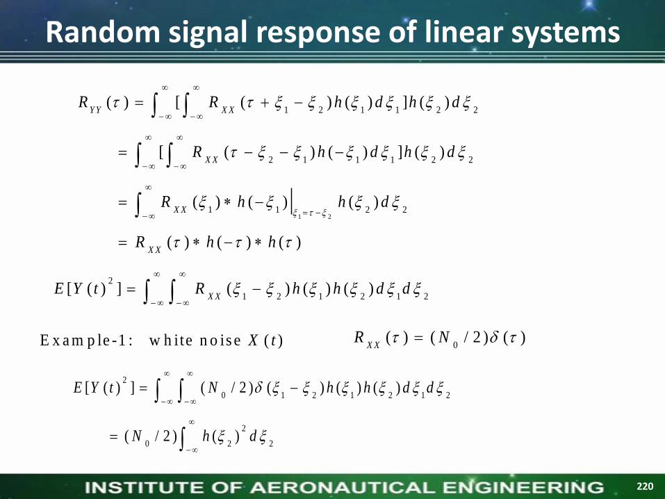
E x a m p le -1 : w h ite n o is e ( )X t 0( ) ( / 2 ) ( )
X XR N
2
0 1 2 1 2 1 2
2
0 2 2
[ ( ) ] ( / 2 ) ( ) ( ) ( )
( / 2 ) ( )
E Y t N h h d d
N h d
1 2
1 2 1 1 2 2
2 1 1 1 2 2
1 1 2 2
( ) [ ( ) ( ) ] ( )
[ ( ) ( ) ] ( )
( ) ( ) ( )
( ) ( ) ( )
Y Y X X
X X
X X
X X
R R h d h d
R h d h d
R h h d
R h h
2
1 2 1 2 1 2[ ( ) ] ( ) ( ) ( )
X XE Y t R h h d d
Random signal response of linear systems
220

( , ) [ ( ) ( ) ] [ ( ) ( ) ( ) ]
[ ( ) ( ) ] ( )
( ) ( )
( ) ( ) ( )
X Y
X X
X X X Y
R t t E X t Y t E X t h X t d
E X t X t h d
R h d
R h R
( ) ( ) ( ) ( ) ( ) ( )
( ) ( )
Y X X Y X X X X
X X
R R R h R h
R h d
( ) w .s .s . ( ) & ( ) jo in t ly w .s .s .X t X t Y t
( ) ( ) ( ) ( ) ( )YY X Y Y X
R R h R h
Random signal response of linear systems
221
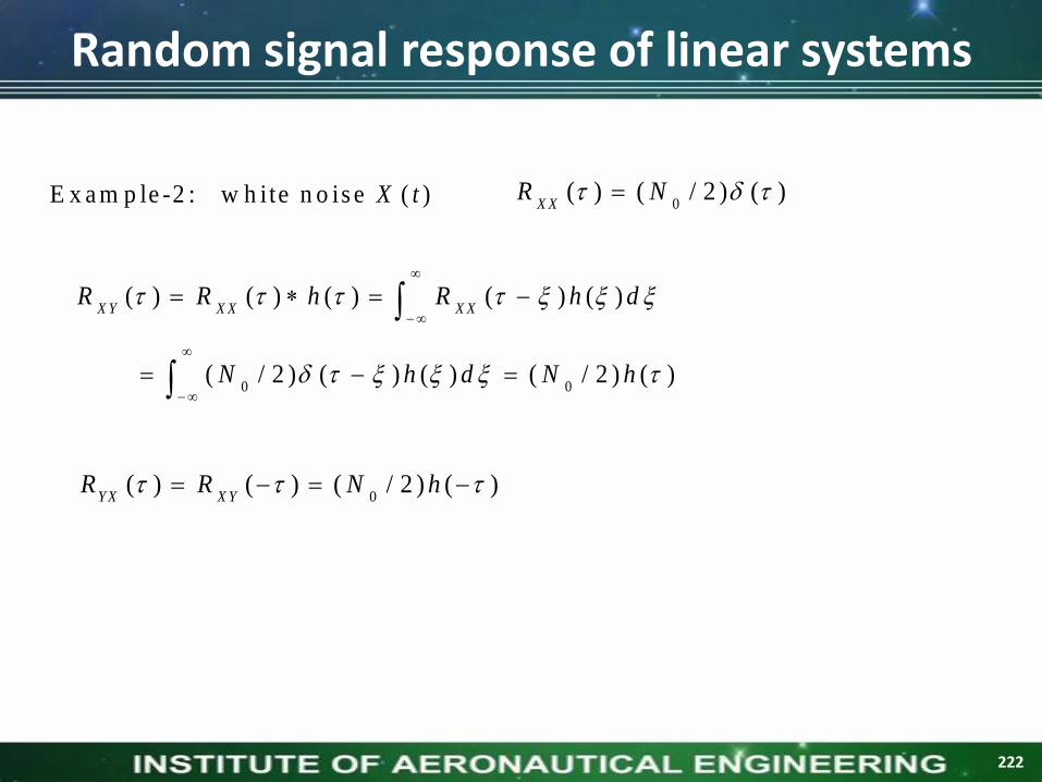
E x a m p le -2 : w h ite n o is e ( )X t 0( ) ( / 2 ) ( )
X XR N
0 0
( ) ( ) ( ) ( ) ( )
( / 2 ) ( ) ( ) ( / 2 ) ( )
X Y X X X XR R h R h d
N h d N h
0( ) ( ) ( / 2 ) ( )
Y X X YR R N h
Random signal response of linear systems
222

Spectral characteristics of system response
( ) ( ) ( )X Y X X
R R h ( ) ( ) ( )X Y X X
S S H
*( ) ( ) ( ) ( ) ( )
Y X X X X XS S H S H
2* *( ) ( ) ( ) ( ) ( ) ( ) ( ) ( )
Y Y X Y X X X XS S H S H H S H
( ) ( )F T
h H
*( ) ( ) ( )
F Th H H ( ) re a l h
( ) ( ) ( )Y X X X
R R h
( ) ( ) ( ) ( ) ( ) ( )Y Y X Y X X
R R h R h h
223

20
2
/ 2( ) ( ) ( )
1 ( / )Y Y X X
NS S H
L R
21 1( ) ( ) ( )
2 2Y Y Y Y X X
P S d S H d
averag e p o w er
E x a m p le -1 :0
( )2
X X
NS
1( )
1 ( / )H
j L R
0
2
/ 2 / 220 0 0
2/ 2 / 2
1 1( )
2 4 1 ( / )
1s e c
4 1 ta n 4 4
Y Y Y Y
NP S d d
L R
N N R N RRd d
L L L
Spectral characteristics of system response
224

1( )
1 ( / )H
j L R
2 2 2 / 2 /0 0 0 0
00
( ) ( / )2 2 4 4
R t L R t L
Y Y
N N N R N RP h t d t R L e d t e
L L
/( ) ( / ) ( )
F TR t Lh t R L u t e
B y E x a m p le -1 ,
Spectral characteristics of system response
225

where h(t) is the impulse response of the system
If E[X(t)] is finiteand system is stable
If X(t) is stationary,H(0) :System DC response.
111 )()()( d ττtXτhtY
-
1 1 1
1 1 1
1 1 1
( ) ( )
( ) ( )
( ) ( )
( ) ( )
Y
-
-
X-
μ t E Y t
E h τ X t τ d τ
h τ E x t τ d τ
h τ μ t τ d τ
1 1
( ) (0 ) ,
Y X X-
μ μ h τ d τ μ H
Random process through a LTI System
226
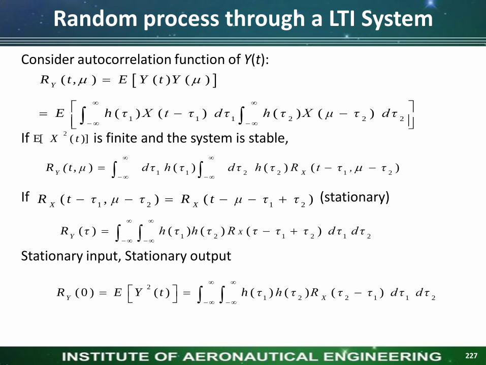
Consider autocorrelation function of Y(t):
If is finite and the system is stable,
If (stationary)
Stationary input, Stationary output
1 1 1 2 2 2
( ) ( ) ( )
( ) ( ) ( ) ( )
Y
R t, E Y t Y
E h τ X t τ d τ h τ X μ τ d τ
)](E[
2tX
1 1 2 2 1 2
) ( ) ( ) ( )
Y XR (t, μ d τ h τ d τ h τ R t τ , τ
)(),(2121
ττμtRτμτtRXX
1 2 1 2 1 2
( ) ( ) ( ) ( )
X Y
R τ h τ h τ R τ τ τ d τ d τ
2
1 2 2 1 1 2(0 ) ( ) ( ) ( ) ( )
Y X
R E Y t h τ h τ R τ τ d τ d τ
Random process through a LTI System
227

Consider the Fourier transform of g(t),
Let H(f ) denote the frequency response,
dfπftjfGtg
dtπftjtgfG
)2exp()()(
)2exp()()(
1 1
2
1 2 2 1 1 2
2
( ) ( ) e x p ( 2 )
( ) ( ) e x p ( 2 ) ( ) ( )
( ) (
X
h τ H f j π fτ d f
E Y t H f j fτ d f h τ R τ τ d τ d τ
d f H f d τ h τ
2 2 1 1 1
2 2 2
) e x p ( 2 )
( ) e x p ( 2 ) ( ) e x p ( 2 )
X
X
R (τ τ ) j fτ d τ
d f H f d τ h (τ ) j fτ R j fτ d
( ) (c o m p le x c o n ju g a te re s p o n s e o f th e f i lte r)*
H f
12 -
Power Spectral Density (PSD)
228

: the magnitude response
Define: Power Spectral Density ( Fourier Transform of )
Recall
Let be the magnitude response of an ideal narrowband filter
D f : Filter Bandwidth
22( ) ( ) ) e x p ( 2 )
X- -
E Y t d f H f R ( τ j f d τ
)( fH
)τR(
22
( ) ( ) ex p ( 2 )
( ) ( ) ( )
X X-
X-
S f R π fτ d
E Y t H f S f d f
2
1 2 1 1 2( ) ( ) ( ) X
- -
E Y t h τ R τ τ d τ d τ
W/Hz in )(Δ2)(
,continuous is )( andΔ If
2
cX
Xc
ff StYE
fSff
)( fH
ff,
ff,|f|H
f
f
c
c
2
1
2
1
0
1)(
Power Spectral Density (PSD)
229

1 2 1 2 1 2
1 2 1 2 1 2
1 2 0 0 1 2
1
( ) ( ) ( ) ( )
( ) ( ) ( ) ( ) e x p ( 2 )
, o r
( ) ( )
Y X
Y X
Y
R h h R d d
S f h h R j f d d d
L e t
S f h h
2 1 0 2 0 1 2 0
2
( ) ( ) e x p ( 2 ) e x p ( 2 ) e x p ( 2 )
( ) ( ) * ( )
( ) ( )
X
X
X
R j f j f j f d τ d τ d τ
S f H f H f
H f S f
h(t)
X(t)
SX (f)
Y(t)
SY (f)
The PSD of the Input and Output Random Processes
230

Let x(t) be a sample function of a stationary and ergodic Process X(t).
In general, the condition for Fourier transformable is
This condition can never be satisfied by any stationary x(t) with infinite duration.
We may write
If x(t) is a power signal (finite average power)
Time-averaged autocorrelation periodogram function
( , ) ( ) e x p ( 2 )
E rg o d ic T a k e tim e a v e ra g e
1 ( ) lim ( ) ( )
2
T
T
T
XTT
X f T x t j f t d t
R x t x t d tT
( ) x t d t
21 1( ) ( ) ( , )
2 2 T
T
T
x t x t d t X f TT
Relation Among The PSD and The Magnitude Spectrum of a Sample Function
231

Take inverse Fourier Transform
we have
Note that for any given x(t) periodogram does not converge asSince x(t) is ergodic
is used to estimate the PSD of x(t)
21 1( ) ( ) ( , ) ex p ( 2 )
2 2
T
T
x t x t d t X f T j fT d fT
21( ) lim ( , ) ex p ( 2 )
2X
T
R X f T j f d fT
T
Relation Among The PSD and The Magnitude Spectrum of a Sample Function
)2exp()(2
1lim
),(2
1lim)(
)2exp()()(
)2exp()(2
1lim)(
)2exp()(2
1lim)()(
2
2
2
2
T
TT
TX
XX
TX
TXX
dtftjtxET
TfXET
fS
dffjfSR
dffjTfXET
R
dffjTfXET
RRE
232

Cross-Spectral Densities
( ) ( ) e x p ( 2 )
( ) ( ) e x p ( 2 )
( ) a n d ( ) m a y n o t b e re a l.
( ) ( ) e x p ( 2 )
( ) ( ) e
X Y X Y
Y X Y X
X Y Y X
X Y X Y
Y X Y X
S f R j f d
S f R j f d
S f S f
R τ S f j π fτ d f
R τ S f
x p ( 2 )
( ) ( )
( ) ( ) ( )
X Y Y X
X Y Y X Y X
j π fτ d f
R τ R τ
S f S f S f
233
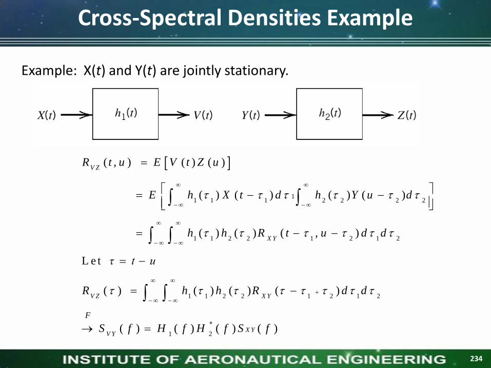
Example: X(t) and Y(t) are jointly stationary.
11 1 1 2 2 2 2
1 1 2 2 1 2 1 2
1 1 2 2 1 2 1 2
( , ) ( ) ( )
( ) ( ) ( ) ( )
( ) ( ) ( , )
L e t
( ) ( ) ( ) ( )
V Z
X Y
V Z X Y
V Y
F
R t u E V t Z u
E h X t d h Y u d
h h R t u d d
τ t u
R h h R d d
S
1 2( ) ( ) ( ) ( )X Yf H f H f S f
Cross-Spectral Densities Example
234
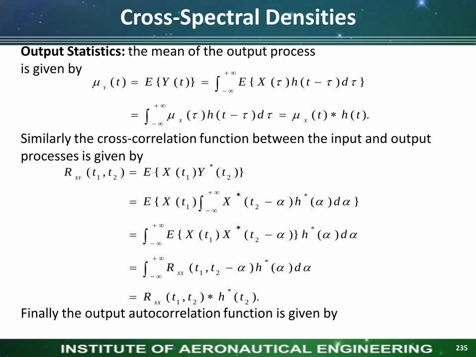
Output Statistics: the mean of the output processis given by
Similarly the cross-correlation function between the input and outputprocesses is given by
Finally the output autocorrelation function is given by
).()()()(
})()({)}({)(
thtdth
dthXEtYEt
XX
Y
).(),(
)(),(
)()}()({
})()()({
)}()({),(
2
*
21
*
21
*
21
*
21
2
*
121
thttR
dhttR
dhtXtXE
dhtXtXE
tYtXEttR
XX
XX
XY
*
*
Cross-Spectral Densities
235

or
),(),(
)(),(
)()}()({
})( )()({
)}()({),(
121
21
21
2
*
1
2
*
121
thttR
dhttR
dhtYtXE
tYdhtXE
tYtYEttR
XY
XY
YY
*
).()(),(),(12
*
2121ththttRttR
XXYY
h(t))( tX
)( tY
h*(t2) h(t1) ),(
21ttR
XY ),(21
ttRYY
),(21
ttRXX
(a)
(b)
Cross-Spectral Densities
236

In particular if X(t) is wide-sense stationary, then we haveso that
Also so that reduces to
Thus X(t) and Y(t) are jointly w.s.s. Further, the output autocorrelation simplifies to
we obtain
XXt )(
constant.a cdhtXXY
,)()(
)(),(2121
ttRttRXXXX
).()()(
,)()(),(21
2121
YYXY
XYYY
RhR
ttdhttRttR
).()()()(*
hhRRXXYY
. ),()()(
)()(),(
21
*
*
2121
ttRhR
dhttRttR
XYXX
XXXY
Cross-Spectral Densities
237

the output process is also wide-sense stationary. This gives rise to the following representation
LTI systemh(t)
Linear system
wide-sense stationary process
strict-sense stationary process
Gaussianprocess (alsostationary)
wide-sense stationary process.
strict-sensestationary process(see Text for proof )
Gaussian process(also stationary)
)( tX )( tY
LTI systemh(t)
)( tX
)( tX
)( tY
)( tY
(a)
(b)
(c)
Cross-Spectral Densities
238

W(t) is said to be a white noise process if
i.e., E[W(t1) W*(t2)] = 0 unless t1 = t2.W(t) is said to be wide-sense stationary (w.s.s) white noise if E[W(t)] = constant, and
If W(t) is also a Gaussian process (white Gaussian process), then all of its samples are independent random variables
For w.s.s. white noise input W(t), we have
),()(),(21121
tttqttRWW
).()(),(2121
qttqttRWW
White noiseW(t)
LTIh(t)
C o lo re d n o ise
( ) ( ) ( )N t h t W t
White Noise Process
239

and
where
Thus the output of a white noise process through an LTI system represents a (colored) noise process.Note: White noise need not be Gaussian.
“White” and “Gaussian” are two different concepts!
)()()(
)()()()(
*
*
qhqh
hhqRnn
.)()()()()(
**
dhhhh
[ ( ) ] ( ) ,
WE N t h d
a con stan t
White Noise Process
240
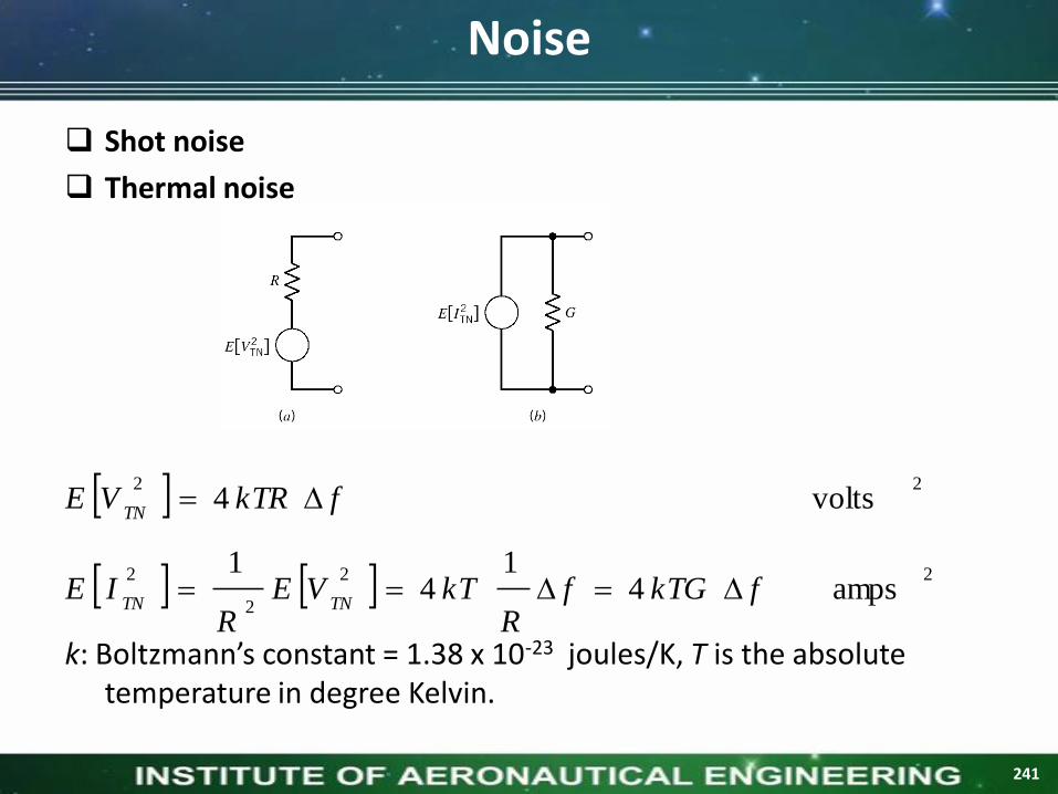
Shot noise
Thermal noise
k: Boltzmann’s constant = 1.38 x 10⁻²³ joules/K, T is the absolute temperature in degree Kelvin.
22
2
2
22
amps 41
41
volts 4
fkTGfR
kTVER
IE
fkTRVE
TNTN
TN
Noise
241

·
)(2
)(
receiver theof re temperatunoise equivalent:
2
)(
0
0
0
N
R
T
kTN
NfS
W
e
e
W
White noise
242

Ideal Low-Pass Filtered White Noise
)2sinc(
)2exp(2
)(
0
2)(
0
0
0
BBN
df fjN
R
B f
B f-B N
fS
B
BN
N
243

Correlation of White Noise with a Sinusoidal Wave
2
)2(cos
)2cos()2cos()(2
2
)2cos()2cos(),(2
)2cos()2cos()()(2
)2cos()()2cos()(2
is )( of varanceThe
)2cos()(2
)('
0
020
210 0
2121
02
210 0
2121
210 0
2121
210 0
2211
2
0
T
c
T T
cc
T T
ccW
T T
cc
T T
cc
T
c
N dtt f
T
N
dt dtt ft fttN
T
dt dtt ft fttRT
dt dtt ft ftwtwET
dt dtt ftwt ftwT
E
tw'
dttftwT
tw
X T
dt0
integer is , , )2cos(2
kT
kftf
Tcc
)( tw )( tw'
White noise
244

Two representations
a. in-phase and quadrature components (cos(2 fct), sin(2 fct))
b. envelope and phase
In-phase and quadrature representation
signals pass-low are )( and )(
)2sin()()2cos()()(
tntn
t ftnt ftntn
Q
Q
I
ccI
Narrowband Noise (NBN)
245

1.nI(t) and nQ(t) have zero mean.
2.If n(t) is Gaussian then nI(t) and nQ(t) are jointly Gaussian.
3.If n(t) is stationary then nI(t) and nQ(t) are jointly stationary.
4.
5. nI(t) and nQ(t) have the same variance .
6.Cross-spectral density is purely imaginary.
7.If n(t) is Gaussian, its PSD is symmetric about fc, then nI(t) and nQ(t) are statistically independent.
otherwise
0
, )()()()(
Bf-BffSffSfSfS
cNcN
NNQI
2
0N
otherwise
0
,
)( )(
Bf-BffSffSj
fSfS
cNcN
NNNNIQQI
Important Properties
246

Ideal Band-Pass Filtered White Noise
).2sinc(2)()(
), offactor (a Compare
)2cos()2sinc(2
)2exp()2exp()2sinc(
)2exp(2
)2exp(2
)(
0
0
0
00
BBNRR
fBBN
fj fjBBN
df fjN
df fjN
R
QI
c
c
c
c
NN
c
cc
Bf
Bf
Bf
BfN
247


