
Practical issues in ALM and
Stochastic modelling for
actuaries
Shaun Gibbs FIA
Eric McNamara FFA FIAA
• Demystify some terms
• Issues around model selection
• Awareness of key choices
• Practical problems in model/parameter
selection
• Demystify market-consistency
• Practical problems with market-consistent
valuations
Objectives

Why use Stochastic
Models?
Because we want to
Because we have to
Basel II Prudential
Sourcebook
(UK) IFRS
ICA (UK)
EEV
Target Surplus (Aus)
Guarantees
on UL
products
Optimising
Asset
Allocation
Alternative
Investments –
Risk/Return
Real Options Embedded Options e.g. NNEG

• Mean reversion
• Fat-Tails
• Arbitrage
• Market-Consistent Calibration
Model Features

Mean Reversion Graphically –
Exchange Rates ASD vs USD (1969-present)
0.0000
0.2000
0.4000
0.6000
0.8000
1.0000
1.2000
1.4000
1.6000
31/0
7/6
9
31/0
7/7
0
31/0
7/7
1
31/0
7/7
2
31/0
7/7
3
31/0
7/7
4
31/0
7/7
5
31/0
7/7
6
31/0
7/7
7
31/0
7/7
8
31/0
7/7
9
31/0
7/8
0
31/0
7/8
1
31/0
7/8
2
31/0
7/8
3
31/0
7/8
4
31/0
7/8
5
31/0
7/8
6
31/0
7/8
7
31/0
7/8
8
31/0
7/8
9
31/0
7/9
0
31/0
7/9
1
31/0
7/9
2
31/0
7/9
3
31/0
7/9
4
31/0
7/9
5
31/0
7/9
6
31/0
7/9
7
31/0
7/9
8
31/0
7/9
9
31/0
7/0
0
31/0
7/0
1
31/0
7/0
2
31/0
7/0
3
31/0
7/0
4
31/0
7/0
5
31/0
7/0
6
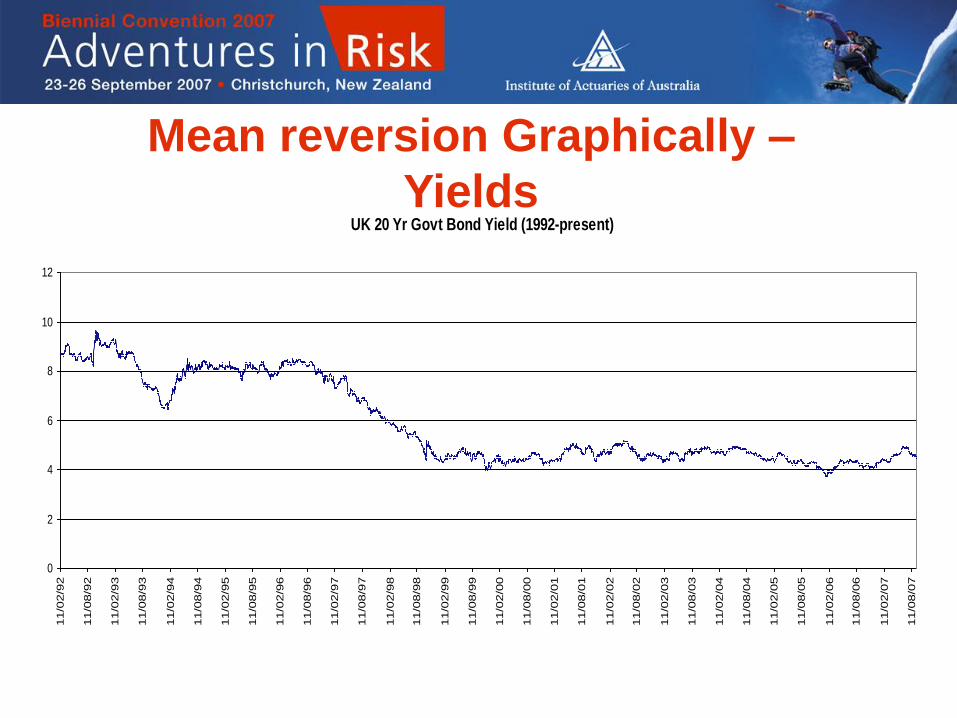
Mean reversion Graphically –
Yields UK 20 Yr Govt Bond Yield (1992-present)
0
2
4
6
8
10
12
11/0
2/9
2
11/0
8/9
2
11/0
2/9
3
11/0
8/9
3
11/0
2/9
4
11/0
8/9
4
11/0
2/9
5
11/0
8/9
5
11/0
2/9
6
11/0
8/9
6
11/0
2/9
7
11/0
8/9
7
11/0
2/9
8
11/0
8/9
8
11/0
2/9
9
11/0
8/9
9
11/0
2/0
0
11/0
8/0
0
11/0
2/0
1
11/0
8/0
1
11/0
2/0
2
11/0
8/0
2
11/0
2/0
3
11/0
8/0
3
11/0
2/0
4
11/0
8/0
4
11/0
2/0
5
11/0
8/0
5
11/0
2/0
6
11/0
8/0
6
11/0
2/0
7
11/0
8/0
7

What is the Consensus?
Equity (Capital Values)
Equity (Dividend Yield) Will differ over different
industries
Bond Yields At least a band of activity
Inflation Developed countries –
Inflation targeting
Exchange Rates Possibly – PPP arguments
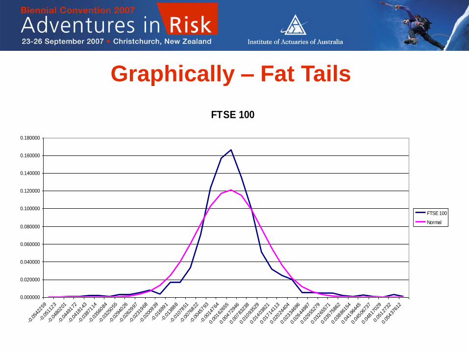
Graphically – Fat Tails
FTSE 100
0.000000
0.020000
0.040000
0.060000
0.080000
0.100000
0.120000
0.140000
0.160000
0.180000
-0.054
2259
-0.051
123
-0.048
0201
-0.044
9172
-0.041
8143
-0.038
7114
-0.035
6084
-0.032
5055
-0.029
4026
-0.026
2997
-0.023
1968
-0.020
0939
-0.016
991
-0.013
888
-0.010
7851
-0.007
6822
-0.004
5793
-0.001
4764
0.00
16265
5
0.00
47294
6
0.00
78323
8
0.01
09352
9
0.01
40382
1
0.01
71411
3
0.02
02440
4
0.02
33469
6
0.02
64498
7
0.02
95527
9
0.03
26557
1
0.03
57586
2
0.03
88615
4
0.04
19644
5
0.04
50673
7
0.04
81702
9
0.05
12732
0.05
43761
2
FTSE 100
Normal
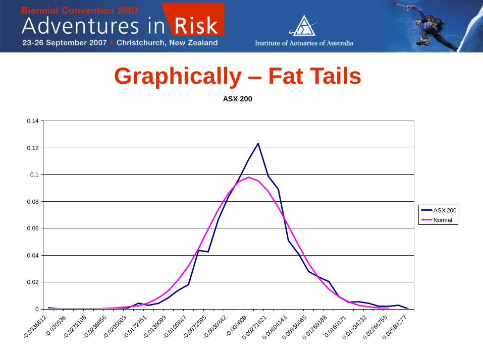
Graphically – Fat Tails ASX 200
0
0.02
0.04
0.06
0.08
0.1
0.12
0.14
-0.0338
612
-0.0305
36
-0.0272
108
-0.0238
856
-0.0205
603
-0.0172
351
-0.0139
099
-0.0105
847
-0.0072
595
-0.0039
342
-0.0006
09
0.00
27162
1
0.00
60414
3
0.00
93666
5
0.01
26918
8
0.01
60171
0.01
93423
2
0.02
26675
5
0.02
59927
7
ASX 200
Normal

• A model that produces outputs permitting
arbitrage opportunities implies that the user
can predict certain future profits
• Modern models produce arbitrage-free
outcomes e.g. yield curves
Arbitrage-Free
• Much demand for models that can produce
market-consistent valuations
• That is, the ability to calibrate the model to
current market prices
• Some models (e.g. The Smith Model, Barrie
& Hibbert) are designed to incorporate MC
calibrations
• Older ones e.g. Wilkie are not
• Importance depends on purpose of modelling
Market-Consistent Calibration

Impact of Model Choice
Source: Creedon S (and 10 other authors), 2003 “Risk and Capital Assessment and Supervision in Financial Firms”,
Interim Working Party Paper, Finance and Investment Conference 2003.

Impact of Model Choice
Source: Creedon S (and 10 other authors), 2003 “Risk and Capital Assessment and Supervision in Financial Firms”,
Interim Working Party Paper, Finance and Investment Conference 2003.
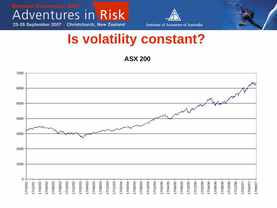
Is volatility constant?
ASX 200
0
1000
2000
3000
4000
5000
6000
7000
17/1
0/0
1
17/1
2/0
1
17/0
2/0
2
17/0
4/0
2
17/0
6/0
2
17/0
8/0
2
17/1
0/0
2
17/1
2/0
2
17/0
2/0
3
17/0
4/0
3
17/0
6/0
3
17/0
8/0
3
17/1
0/0
3
17/1
2/0
3
17/0
2/0
4
17/0
4/0
4
17/0
6/0
4
17/0
8/0
4
17/1
0/0
4
17/1
2/0
4
17/0
2/0
5
17/0
4/0
5
17/0
6/0
5
17/0
8/0
5
17/1
0/0
5
17/1
2/0
5
17/0
2/0
6
17/0
4/0
6
17/0
6/0
6
17/0
8/0
6
17/1
0/0
6
17/1
2/0
6
17/0
2/0
7
17/0
4/0
7
17/0
6/0
7

Is volatility constant? ASX 200 - % Daily movement
-4.00%
-3.00%
-2.00%
-1.00%
0.00%
1.00%
2.00%
3.00%
4.00%
18/1
0/0
1
18/1
2/0
1
18/0
2/0
2
18/0
4/0
2
18/0
6/0
2
18/0
8/0
2
18/1
0/0
2
18/1
2/0
2
18/0
2/0
3
18/0
4/0
3
18/0
6/0
3
18/0
8/0
3
18/1
0/0
3
18/1
2/0
3
18/0
2/0
4
18/0
4/0
4
18/0
6/0
4
18/0
8/0
4
18/1
0/0
4
18/1
2/0
4
18/0
2/0
5
18/0
4/0
5
18/0
6/0
5
18/0
8/0
5
18/1
0/0
5
18/1
2/0
5
18/0
2/0
6
18/0
4/0
6
18/0
6/0
6
18/0
8/0
6
18/1
0/0
6
18/1
2/0
6
18/0
2/0
7
18/0
4/0
7
18/0
6/0
7

• Many approaches to deal with non-constant
volatility:
• ARCH family: Error term is heteroscedastic and
auto-correlated, allowing “runs” of high and low
volatility
• Ornstein-Uhlenbeck: Model volatility as a mean
reverting stochastic process
• Markov regime switching: Model economy as
having states with varying volatility
characteristics. Transition matrices govern
movements between states
Modelling Volatility

• Reverse Mortgages incorporate the No Negative- Equity
Guarantee – an embedded put option for the borrower
• Our risky assets here are:
– The value of the Property
– Short term interest rates (if loan is variable rate)
• Valuing this put option require a property model
• How volatile is an individual house price?
• How does volatility differ between geographical areas?
• Some data available on mean house prices, but moving
prices for an individual property not available
• One solution is to merge knowledge of volatility in mean
price index and distribution of price around mean
A Topical Problem – Implied Volatility

• Stochastic programming allows us to incorporate
contingent events within each simulation
• Some Examples:
– Policyholder decisions: Lapses/renewals/new
business/policy conversions related to economic
conditions
– Management decisions: Asset allocation, premium
rates, closure to NB
• Modelling policyholder decisions means fully allowing for
contingent risks
• Modelling management decisions means allowing for
reasonably foreseeable action, usually to prevent
insolvency or improve performance
Dynamic Decisions

• Some considerations:
• Contingent actions of policyholders need to have
credible backing evidence
• Management decisions need to be based on
business plans, contingency arrangements and
best-practice
• Need to allow for any delays in action i.e. cure
unlikely to be applied instantaneously
Dynamic Decisions (contd)
• The concept of market consistent valuation is here
to stay. Areas of application include International
Financial Reporting Standards (IFRS), European
Embedded Value (EEV) and Solvency II
• In essence, the concept is to place a value on
liabilities in a manner which is consistent with
how the market prices comparable financial
instruments
Market consistent valuations (MCV)
Not when you break it down to basics……
• MCV of an annuity requires the matching bonds
• MCV of a capital guaranteed bond requires the
underlying asset plus a suitable put option
Market prices of comparable
market instruments sounds very
fancy!!

• This is a common scenario
• Then we must use financial mathematics to derive
or model a synthetic replication to come up with a
MCV
2 main methods exist. They are:
• Real world methods with deflators
• Risk neutral methods
Comparable instrument or
‘replicating asset’ may not exist

• Is there a replicating asset?
• Are we calibrated to the market?
• Are we arbitrage free (there should be a unique
price for an asset)?
• Do we use risk neutral or real world?
Key points of MCV
• Real world techniques involve projecting realistic
cashflows and using deflators to discount them
• Deflators are essentially stochastic discount
functions
Traditional PV of cashflow = Vt E[ Ct]
MCV PV of cashflow = E[ Vt Ct]
Real world – realistic cashflows

• The probabilities in the expected cashflows in
real world are realistic but in risk neutral they
are adjusted ‘risk neutral’ probabilities
• Rather than apply a deflator to value a cashflow,
the risk neutral approach uses the risk-free rate
The MCV should be the same whether we use
real or risk neutral
Risk neutral – risk adjusted
cashflows
Real world
+ Cashflows can be used for planning/forecasting
+ Real world method is more transparent
+ Potentially quicker as only one model required for
valuation and planning results
- Mathematically more complicated as deflators are
required
- More difficult to calibrate to the market due to the
complexity involved
- Harder to understand and explain
Comparison of approaches

Risk Neutral
+ A mathematically simpler approach to achieving a market
consistent valuation
+ Easier to calibrate to market
+ Results are easier to explain as based on risk free rates
and not deflators
+ More understood as banks have been using this method
for some time
- Cashflows are not the realistic expected cashflows and so
cannot be used for planning/forecasting
- Must run two models, one for valuation and one for
cashflow projections
It depends!
Both approaches will give the same value result.
Really depends on the purpose of the valuation i.e.
is it say checking solvency at a point in time? Or is
it a planning exercise that requires realistic
cashflows?
Which method is best?
• Objectivity? Still have to choose a statistical
distribution. Still have to think about tails,
reversion etc. Subjective?
• Incomplete/inefficient markets – as highlighted in
‘Deflators Demystified’ by Joshua Corrigan et al
(2007). In such cases we cannot reliably model in
a MC fashion
Other issues to think about
• Being objective as calibrated by the market?
• Prevent any issues such as artificial value creation
through changing the asset mix.
• Produce a fair value of liabilities
• Place an appropriate value on options and
guarantees
Why bother with MCV?
• The MCV approach is becoming popular in AV/EV/EEV
work. In particular, EEV methodology was born to
enhance the consistency between EV results in Europe.
The MCV approach is a natural choice for this as:
• Removes subjectivity in results caused by selection of a
risk discount rate
• More appropriate modelling of the cost of guarantees and
options
• Does not allow the creation of value by changing the
asset mix
Practical application of MCV

• MCV methodologies only address systematic risk. MCV
assumes that all unsystematic risks are diversifiable as in
pure financial theory
• However, development in this area has shown there is a
cost/reward for these unsystematic risks in the form of
frictional costs. These frictional costs are often used as
the balancing item to explain the differences between
MCV and traditional methods
Frictional costs
Main sources are as follows:
• Agency costs - management decisions
• Cost of financial distress - financial difficulties
• Transaction costs - salaries etc
• Neutrality of taxes - asymmetric taxes
Frictional costs
• We have shown that you can calibrate to the
market for investment returns but how do you
calibrate to market growth rates for life insurance
business?
• This is more of an issue in situations where the
value of future new business is significant. And
this is often the case in the Australian market
MCV AVs – the problem with new
business

• There is no obvious method to calculate a market
consistent growth rate. Therefore, when applying
a new business multiplier we need to think of how
the growth rate will vary with the market
• Wealth management products positively
correlated with market………risk products less
so……..others?
MCV AVs – the problem with new
business
• In a traditional appraisal value, a single discount
rate is often applied to both the inforce and new
business. This discount rate includes implicit
allowances for business risks including the risks
associated with selling new business
• Effectively, this means that both the EV and new
business have a value reduction
MCV AVs – the problem with new
business

• In a MCV AV, by definition, there is only
allowance for market risk. Therefore, an
adjustment is required to be made to the new
business component to allow for the unsystematic
new business risk
• Unlike a traditional method, this value reduction
will be captured completely in the new business
value
MCV AVs – the problem with new
business

• Therefore, all else being equal, the market
consistent multiplier will potentially be lower
than the corresponding traditional multiplier.
However, to what degree is difficult to quantify
• The real solution lies in the ability to develop a
stochastic growth rate with a distribution that is
based on market data. This most likely means a
different new business multiplier for each product
type
MCV AVs – the problem with new
business
• HOW??? Calibrate to what? No suitable assets
exist
• Proxy MCV to calibrate to recent market
transactions. A workaround and not MC in the
true sense
• We require a method to derive an appropriate
level of correlation between growth rates and the
market returns
MCV AVs – the problem with new
business

Questions????


