

Ç.Ü. Sosyal Bilimler Enstitüsü Dergisi, Cilt 25, Sayı 2, 2016, Sayfa 41-56
41
PREDICTION OF CENTRAL GOVERNMENT BUDGET TAX REVENUES
USING MARKOV MODEL
Merkezi Bütçe Vergi Gelirlerinin Markov Modeli ile Tahmin Edilmesi
Can Mavruk*
Ersin KIRAL**
ABSTRACT
The aim of this paper is to describe the behavior of the sample data and to
predict the realization rates of tax revenues by one step stochastic Markov chain model.
The realization rates of the tax revenues are estimated by using 2000-2014 gross annual
data extracted from TR Revenue Administration. Four Markov models are constructed
for the realization rates of every tax revenue. The realization probabilities for the year
2016 are predicted by constructing probability matrices of transitions between classes
described for every model. Revenues are also forecasted by the product of the initial
probability matrix and transition probability matrix. Limiting matrix of predictions are
found. The best Markov model was found by estimating the sum of mean square errors
for every model. The results are compared and interpreted.
Keywords: Tax Revenues, Transition Probabilities, Markov Analysis, Budget Forecast
ÖZET
Bu makalenin amacı örnek verinin davranışını tanımlamak ve bir adımlı
stokastik Markov zinciri modeli ile vergi gelirleri kalemlerinin gerçekleşme oranlarını
tahmin etmektir. Gelir İdaresi Başkanlığı 2000-2014 brüt yıllık verileri kullanılarak
vergi gelirlerinin gerçekleşme olasılığı hesaplanmıştır. Her verginin gerçekleşme
oranları için dört Markov modeli oluşturulmuştur. Her model için belirlenen sınıflar
arası geçiş olasılıkları matrisleri oluşturularak 2016 yılı gerçekleşme olasılıkları tahmin
edilmiştir. Ayrıca gelirler başlangıç matrisi ve geçiş olasılıkları matrisinin çarpımı ile
tahminlenmiştir. Tahminlerin limit matrisleri bulunmuştur. En iyi Markov modeli hata
karelerinin ortalamasının hesaplanmasıyla bulunmuştur. Sonuçlar karşılaştırılarak
yorumlanmıştır.
Anahtar Kelimeler: Vergi gelirleri, Geçiş Olasılıkları, Markov Analizi, Bütçe Tahmin
Introduction
Prediction of central government budget tax revenues has a great importance in
planning the distribution of revenues to public expenditures. Tax revenues are generated
from taxes collected from income, property, goods, services and foreign trade. The
proportion of tax incomes in general budget revenues has been increasing
* Öğr.Gör., Lecturer of Mathematics and Statistics, Nigde University, Vocational
School of Social Sciences, [email protected] ** Yrd.Doç.Dr., Assistant Professor of Operations Research, Cukurova University,
School of Business and Economics Dept. of Econometrics, [email protected]

Ç.Ü. Sosyal Bilimler Enstitüsü Dergisi, Cilt 25, Sayı 2, 2016, Sayfa 41-56
42
(www.ekodialog.com>konular>genel_butce 8.12.2015). Even though tax incomes have
increased over time, the realization rates show a decreasing to stationary or increasing to
stationary behavior. Since public expenditures are also increasing by time, an increase
in realization rates is also expected. Otherwise, indirect tax items would be increased to
cover increasing public expenditures, which brings a heavy load to public. Tax increase
and revaluation rates are determined by Turkish Statistical Institute (TUIK) from twelve
month mean of domestic producer price index (dppi) in October
(http://www.zaman.com.tr/ekonomi_2015-yilinda-vergiler-yuzde-1011-oraninda-
artacak_2255169.html 10.12.2015). As of January 1st 2016, motor vehicle tax, stamp
duty tax, environmental tax, fees, traffic fines and tax fines will increse by the
revaluation rate 5.58% unless Council of Ministers increase or decrease this rate
(http://www.hurriyet.com.tr/2016-vergi-artis-oranlari-belli-oldu-40009417 9.12.2016).
Sub-items of tax revenues are individual income tax, corporate income tax, property tax,
inheritance and gift tax, motor vehicle tax, value added tax, special consumption tax,
banking and insurance transaction taxes, tax on wagering, special communication tax,
tax on customs, VAT on imports and stamp duty tax. In this paper, tax revenues are
analyzed and predicted by four Markov Models. The best of the four has the least sum
of the mean square errors. Predictions of tax revenues are expected to be stationary and
to have a limiting matrix.
Literature
Baasch et. al (2010) used Markov models to quantify transitions between
successional stages. They presented a solution for converting multivariate ecological
time series into transition matrices and demonstrate the applicability of this approach for
a data set that resulted from monitoring the succession of sandy dry grassland in a post-
mining landscape. They analyzed five transition matrices, four one-step matrices
referring to specific periods of transition (1995–1998, 1998–2001, 2001–2004, 2004–
2007), and one matrix for the whole study period (stationary model, 1995–2007).
Büyüktatlı et. al (2013) used initial allocations of investment program with
actual spending percentages from the years of 1998-2009 of Turkish Atomic Energy
Institute (TAEK) to predict annual allowances from Ministry of Energy and Natural
Resources. An estimated percentage of realization of investment program for 2011 and
results are interpreted with Markov analysis.
Cavers and Vasudevan (2015) directed graph representation of a Markov chain
model to study global earthquake sequencing leads to a time series of state-to-state
transition probabilities that includes the spatio-temporally linked recurrent events in the
recordbreaking sense. A state refers to a configuration comprised of zones with either the occurrence or non-occurrence of an earthquake in each zone in a pre-determined
time interval. Grimshaw and Alexander (2011) used a Markov chain model to forecast
outstanding balance of loans in each delinquency state. For that they used a markov
chain Xn as the delinquency state of a loan in month n and a Markov Chain model for
loan accounts that are ‘current’ this month having a probability of moving next month
into ‘current’, ‘delinquent’ or ‘paid-off’ states. They forecasted ‘one month ahead’

Ç.Ü. Sosyal Bilimler Enstitüsü Dergisi, Cilt 25, Sayı 2, 2016, Sayfa 41-56
43
portfolio delinquency balance for a portfolio of loans where each loan is ni months from
origination this month i=1,...,N.
Lazri et.al (2015) adopted a Markovian approach to discern the probabilistic
behaviour of the time series of the drought. A transition probability matrix was
constructed from drought distribution maps. Markov transition probability formula for
four states and a simulation model with an initial probability vector was used to
calculate the drought distribution area in the future.
Lukić et. al. (2013) used the stochastic method based on a Markov chain
model to predict the annual precipitation in the territory of South Serbia for the period
2009-2013. For this purpose, the precipitation data rainfall recorded on the four
synoptic stations were used for the period 1980-2010.
Usher (1979) discussed that complex non-random or Markovian processes are
likely to characterize ecological successions, the transition probability matrix elements
not being constant but being functions either of the abundance, or of the rate of change
of abundance, of a recipient class.
Methodology: Markov Model
Markov chain is a stochastic process which is described by a transition matrix
of transition probabilities from one state into another state (Vantika and Pasaribu, 2014,
p.2).
A discrete time process {Xn,n = 0,1,2,...} with discrete state space Xn ∈ {0, 1,
2, ...} is a Markov chain if it has the Markov property: P(Xn+1=j | Xn=i, Xn−1 = in−1, ...,X0
= i0) = P(Xn+1=j|Xn=i) = p(i,j) where p(i,j) depends only on the states i,j, and not on the
time n or the previous states” (dept.stat.lsa.umich.edu/~ionides/620/notes/markov
_chains.pdf 15.12.2015). The numbers p(i,j) are called the transition probabilities of the
chain. (galton.uchicago.edu/~lalley/Courses/312/MarkovChains.pdf 15.12.2015).
One step probability is pij=P(X1=j | X0=i) (İlarslan, 2014, s.6190). In a first
order Markov chain, the state at any time instant depends only on the state immediately
preceding it, and hence is defined as a single-dependence chain and m step probability
is pm
ij =P(Xm=j | X0=i).
Construction of Transition Probabilities
Transition probability matrices are estimated for 2000-2014 for sub-items of
tax revenues. The estimator of the transition probabilities is the relative frequency of the
actual transitions from phase i to phase j, i.e. the observed transitions have to be divided
by the sum of the transitions to all other phases (Lipták, 2011, p.141)
In this paper, j ijijij nnP / where i, j = A, B, C, D, E and nij is the number of
observed transitions from i to j and j ijn is the sum of observed transitions from i to j.
Frequency distribution of the realization rate intervals must be mutually
exclusive (nonoverlapping) and class width must be equal for each interval (Bluman,
2014, p.45-46). Transition probabilities from Xi to Xj, i, j = 0,1,2,…,n, can be
constructed as the following matrix (Taha, 2000, p.726)

Ç.Ü. Sosyal Bilimler Enstitüsü Dergisi, Cilt 25, Sayı 2, 2016, Sayfa 41-56
44
nnnn
n
n
ij
PPP
PPP
PPP
P
...
...
...
21
22221
11211
Since pij are constant and independent of time (time homogeneous), matrix Pij
= P is called a stochastic matrix. Pij probabilities must satisfy the following conditions:
njiPij ,...,2,1,0 nipi
ij ,...,2,11
Prediction
Given that data at time n is in state X0 and that the data will be in one of states
Xn ∈ {0,1,2,...} at time n+1, then the data at time n+2 can be predicted. Given initial
probability P(X0 = i) = pi for every i, the required probability is matrix multiplication pi
kjk ikPP . Equivalently, next year’s probability distribution matrix can be predicted by
Qn+1 = Qn P n = 0,1,2,3,… (1)
Initial probability matrices for four Markov models are 1xj row matrices. Stationary
prediction matrices Qn+1 have a limiting matrix Q, which can be written as QQnn
lim .
Best of Four Markov Models
For every year of the sample and for every Markov model, mean square error
(mse) is calculated by
n
i
ii rrn 1
2ˆ
1 where i is the number of states, nnn PQQ 1
ˆ
nrrrr ˆˆˆˆ321 is predicted realization rate at time n+1 and nn rrrQ 21 is
observed realization rate at time n. The least mse gives the best Markov model.
Statistical Significance of the Models
Variations between observed and expected frequencies can be tested by
constructing a contingency table of frequency distribution of transitions between the
states at 0,05 significance level with a degree of freedom.
To validate Markov model, for every year, the value of the χ2 statistic is
computed based on the null hypothesis, H0: model is valid. At 0,05 level of significance
and with the degrees of freedom, the χ2 critical value and χ
2 test value are estimated.
The null hypothesis is not rejected whenever χ2 test value is less than the critical value.
Test values are calculated by iii i rrr ˆ/)ˆ( 22 where i is the number of
categories, and ir and
ir̂ are the actual and estimated values, respectively.
Income Tax
Income tax targeted, collected (http://www.gib.gov.tr/sites/default/files/fileadmin/user_
upload/VI/GBG/Tablo_47.xls.htm, http://www.gib.gov.tr/sites/default/files/fileadmin/
user_upload/VI/GBG/Tablo_44.xls.htm, http://www.gib.gov.tr/sites/default/files/
fileadmin/user_upload/VI/GBG/Tablo_46.xls.htm, http://www.gib.gov.tr/sites/default

Ç.Ü. Sosyal Bilimler Enstitüsü Dergisi, Cilt 25, Sayı 2, 2016, Sayfa 41-56
45
/files/fileadmin/user_upload/VI/GBG/Tablo_45.xls.htm 5.12.2015) and realization rates
for the years 2000-2014 are given in Table 2. In the last fifteen years the highest rate in
income tax realized was 113,7% in 2001 and the lowest realized was 85.1% in 2009.
Targeted income tax has increased every year except the year 2010. Tax collection has
increased every year between 2000-2014. While targeted income tax was increasing
4,47 billion TL per year on average, tax collection was also increasing 4,88 billion TL
per year on average.
Income Tax Markov Models and Transition Probability Matrices
Income tax realization rates from smallest to largest are classified as E,D,C,B,
A in model 1, D, C, B, A in model 2, C, B, A in model 3 and B, A in model 4. For years
between 2000 and 2014 table 2 shows that realization rates are over 100% in three
categories of model 1, in two categories of model 2, in two categories of model 3.
Table 1. Income Tax Markov Models and Transition Probability Matrices
Markov Model 1 Transition Matrix Markov Model 2 Transition Matrix
Real.Interval (%) A B C D E Real.Interval (%) A B C D
108.3 ≤ r
102.5 ≤ r ≤ 108.2
96.7 ≤ r ≤ 102.4
90.9 ≤ r ≤ 96.6
r ≤ 90.8
A
B
C
D
E
0 1/2 0 0 1/2 106.7 ≤ r A
B
C
D
1/3 1/3 0 1/3
1/5 2/5 2/5 0 0 99.5 ≤ r ≤ 106.6
1/3 1/2 0 1/6
2/5 2/5 0 0 1/5 92.3 ≤ r ≤ 99.4
1/3 2/3 0 0
0 0 0 0 0 r ≤ 92.2
0 0 1 0
0 0 1 0 0
Markov Model 3 Transition Matrix Markov Model 4 Transition Matrix
Real. Interval (%) A B C Real. Interval (%) A B
104.3 ≤ r
A
B
C
2/5 2/5 1/5 99.5 ≤ r
A
B
C
7/9 2/9
94.7 ≤ r ≤ 104.2
4/7 2/7 1/7 r ≤ 99.4 B 3/5 2/5
r ≤ 94.6
0 1 0
For the years 2000-2014, the realization rates of income tax, classes and
transitions for four Markov models are shown in Table 2.
Tablo 2. Income Tax (000 TL) and Classification of Realization Rates and Transitions
Year Targeted Collected
Real.
Rate
(%)
Class M1 Class M2 Class M3 Class M4
2000 6.276.000 6.212.977 99 C C B B
2001 10.186.000 11.579.424 113,7 A CA A CA A BA A BA
2002 15.401.000 13.717.660 89,1 E AE D AD C AC B AB
2003 17.196.918 17.063.761 99,2 C EC C DC B CB B BB
2004 18.655.000 19.689.593 105,5 B CB B CB A BA A BA
2005 21.170.000 22.817.530 107,8 B BB A BA A AA A AA
2006 29.071.000 31.727.644 109,1 A BA A AA A AA A AA
2007 36.922.897 38.061.543 103,1 B AB B AB B AB A AA
2008 38.780.119 39.249.867 101,2 C BC B BB B BB A AA
2009 46.598.274 39.668.595 85,1 E CE D BD C BC B AB
2010 42.927.809 41.969.451 97,8 C EC C DC B CB B BB
2011 48.951.204 51.092.935 104,4 B CB B CB A BA A BA
2012 56.710.510 58.797.752 103,7 B BB B BB B AB A AA
2013 65.483.652 65.914.727 100,7 C BC B BB B BB A AA
2014 73.289.337 79.451.776 108,4 A CA A BA A BA A AA

Ç.Ü. Sosyal Bilimler Enstitüsü Dergisi, Cilt 25, Sayı 2, 2016, Sayfa 41-56
46
Prediction For Income Tax Realization Rate
Given that 2014 income tax realization rate 108.4% is in state A and that income
tax will be in one of states A, B, C, D or E in 2015, income tax realization rate for 2016
is predicted.
Tablo 3. Income Tax Realization Rates Predictions for 2016
Realization
Interval (%)
M1
Pred.
Realization
Interval (%)
M2
Pred.
Realization
Interval (%)
M3
Pred.
Real. Int.
(%)
M4
Pred.
r ≤ 90.8 0 r < 92.2 0.17 r ≤ 94.6 0,14 r ≤ 99.4 0,26
90.9 ≤ r ≤ 96.6 0 92.3 ≤ r ≤ 99.4 0,33 94.7 ≤ r ≤ 104.2 0,47 99.5 ≤ r 0,74
96.7 ≤ r ≤ 102.4 0,70 99.5 ≤ r ≤ 106.6 0,28 104.3 ≤ r 0,39
102.5 ≤ r ≤ 108.2 0,20 106.7 ≤ r 0,22
108.3 ≤ r 0,10
Stationarity of Income Tax Predictions
Predictions are estimated in Excel by formula (1) for all models. According to
four models, all probabilities become stationary in 2031, 2026, 2022 and 2020
respectively.
Statistical Significance of The Model For Income Tax
In model 1 of income tax, variations between observed and expected
frequencies can be tested by constructing a contingency table of frequency distribution
of transitions between the states at 0,05 significance level with 16 df. Since chi square
test value 11,23 is less than critical value 26,296, H0 is not rejected. This shows that
there is no significant variations. The values in paranthesis in the Table 4 are expected
frequencies which are found from (row sum X column sum)/total. Table 4 shows that in
model 1 transitions in higher realization states are stable and in lower states rates are
improving.
Table 4. Contingency Table of Observed and Expected Income Tax Rates of Model 1. A B C D E Total
A 0 (0,43) 1 (0,71) 0 (0,57) 0 1 (0,29) 2
B 1 (1,07) 2 (1,79) 2 (1,43) 0 0 (0,71) 5
C 2 (1,07) 2 (1,79) 0 (1,43) 0 1 (0,71) 5
D 0 0 0 0 0 0
E 0 (0,43) 0 (0,71) 2 (0,57) 0 0 (0,29) 2
Total 3 5 4 0 2 14
Corporate Tax
Corporate tax targeted, collected and realization rates for years 2000-2014 are
given in Table 6. In the last fifteen years the highest corporate tax rate realized was
175% in 2001 when targeted at the lowest and the lowest realized was 71,2 in 2000.
Targeted corporate tax has increased every year except the years 2001, 2005, 2007 and
2010. Tax collection has increased every year between 2000-2014 except in 2013 when
it had a slight decrease. While targeted corporate tax was increasing 2 billion TL per
year on average, tax collection was also increasing 2,2 billion TL per year on average.

Ç.Ü. Sosyal Bilimler Enstitüsü Dergisi, Cilt 25, Sayı 2, 2016, Sayfa 41-56
47
But, the realization rate was decreasing by approximately 1,5% per year in the given
period.
Corporate Tax Transition Probability Matrices
In four categories of model 1, in three categories of model 2, in all categories
of model 3 and model 4, realization rates are over 100% between 2000 and 2014.
Table 5. Corporate Tax Markov Models and Transition Probability Matrices
Markov Model 1 Transition Matrix Markov Model 2 Transition Matrix
Real.Interval (%) A B C D E Real. Interval (%) A B C D
154,4 ≤ r
133,6 ≤ r ≤ 154,3
112,8 ≤ r ≤ 133,5
92 ≤ r ≤ 112,7
r ≤ 91,9
A
B
C
D
E
.5 0 0 .5 0 149,2 ≤ r A
B
C
D
.5 0 .5 0
0 0 0 0 0 123,2 ≤ r ≤ 149,1 0 0 0 1
0 0 1/3 1/3 1/3 97,2 ≤ r ≤ 123,1 0 1/7 5/7 1/7
0 0 1/6 4/6 1/6 r ≤ 97,1 1/4 0 3/4 0
1/3 0 1/3 1/3 0
Markov Model 3 Transition Matrix Markov Model 4 Transition Matrix
Real. Interval (%) A B C Real. Interval (%) A B
140,8 ≤ r A
B
C
.5 0 .5 123,2 ≤ r A
B
C
1/3 2/3
105,8 ≤ r ≤ 140,7 0 .5 .5 r ≤ 123,1 B 2/11 9/11
r ≤ 105,7 1/6 1/2 1/3
For the years 2000-2014, the realization rates of corporate tax, classes and
transitions for four Markov models are shown in Table 6.
Table 6. Corporate Tax (000 TL) and Classification of Realization Rates and Transitions
Year Targeted Collected Real.
Rate
(%)
Class MM1 Class MM2 Class MM3 Class MM4
2000 3.309.000 2.356.787 71,2 E D C B
2001 2.100.000 3.675.665 175 A EA A DA A CA A BA
2002 3.595.000 5.575.495 155,1 A AA A AA A AA A AA
2003 8.918.160 8.645.345 96,9 D AD D AD C AC B AB
2004 9.335.000 9.619.359 103 D DD C DC C CC B BB
2005 8.890.000 11.401.986 128,3 C DC B CB B CB A BA
2006 14.756.000 12.447.354 84,4 E CE D BD C BC B AB
2007 14.410.186 15.718.474 109,1 D ED C DC B CB B BB
2008 16.976.161 18.658.195 109,9 D DD C CC B BB B BB
2009 22.611.359 20.701.805 91,6 E DE D CD C BC B BB
2010 20.071.108 22.854.846 113,9 C EC C DC B CB B BB
2011 25.359.580 29.233.725 115,3 C CC C CC B BB B BB
2012 30.035.121 32.111.820 106,9 D CD C CC B BB B BB
2013 32.043.560 31.434.581 98,1 D DD C CC C BC B BB
2014 33.892.413 35.163.517 103,8 D DD C CC C CC B BB

Ç.Ü. Sosyal Bilimler Enstitüsü Dergisi, Cilt 25, Sayı 2, 2016, Sayfa 41-56
48
Realization Rates and Transition Probability Matrices of Other Tax Revenues
Table 7. Property Tax Markov Models and Transition Probability Matrices
Markov Model 1 Transition Matrix Markov Model 2 Transition Matrix
Real.Interval (%) A B C D E Real. Interval (%) A B C D
134,5 ≤ r
123,1 ≤ r ≤ 134,4
111,7 ≤ r ≤ 123
100,3 ≤ r ≤ 111,6
r ≤ 100,2
A
B
C
D
E
0 0 0 .5 .5 r ≤ 103 A
B
C
D
0 0 .5 .5
0 0 0 0 0 103,1 ≤ r ≤ 117,2 0 0 0 0
0 0 0 1 0 117,3 ≤ r ≤ 131,4 0 0 .25 .75
0 0 0 .4 .6 131,5 ≤ r 1/8 0 1/8 6/8
1/6 0 1/6 1/6 3/6
Markov Model 3 Transition Matrix Markov Model 4 Transition Matrix
Real. Interval (%) A B C Real. Interval (%) A B
r ≤ 103 A
B
C
0 0 1 117,3 ≤ r
A
B
C
0 1
103,1 ≤ r ≤ 117,2 0 0 1 r ≤ 117,2
B 1/12 11/12
117,3 ≤ r ≤ 131,4 1/11 1/11 9/11
Table 8. Inheritance and Gift Tax Markov Models and Transition Probability Matrices
Markov Model 1 Transition Matrix Markov Model 2 Transition Matrix
Real.Interval (%) A B C D E Real. Interval (%) A B C D
125,7 ≤ r
108,6 ≤ r <125,6
91.5 ≤ r < 108,5
74,4 ≤ r < 91,4
r < 74,3
A
B
C
D
E
1/3 0 2/3 0 0 121,5 ≤ r A
B
C
D
.25 .75 0 0
0 1/3 1/3 0 1/3 100,1 ≤ r ≤ 121,4
.2 .4 .2 .2
2/5 1/5 2/5 0 0 78,7 ≤ r ≤ 100
1 0 0 0
0 0 0 0 0 r ≤ 78,6 0 1/3 1/3 1/3
0 1/3 1/3 0
/
6
1/3
Markov Model 3 Transition Matrix Markov Model 4 Transition Matrix
Real. Interval (%) A B C Real. Interval (%) A B
114,1 ≤ r
A
B
C
1/3 1/2 1/6 100,1 ≤ r
A
B
C
7/9 2/9
85,8 ≤ r ≤ 114,2
3/5 2/5 0 r ≤ 100 B 3/5 2/5
r ≤ 85,7 1/3 1/3 1/3
Table 9. Motor Vehicle Tax Markov Models and Transition Probability Matrices
Markov Model 1 Transition Matrix Markov Model 2 Transition Matrix
Real.Interval (%) A B C D E Real.Interval (%) A B C D
110,8 ≤ r
105,5 ≤ r ≤110,7
100,2 ≤ r ≤105,4
94,9 ≤ r ≤ 100,1
r ≤ 94,8
A
B
C
D
E
0 0 1 0 0 109,7 ≤ r A
B
C
D
0 0 1 0
0 .5 .25 .25 0 103 ≤ r ≤109,6
0 4/5 1/5 0
0 0 4/6 2/6 0 96,3 ≤ r ≤ 102,9
0 0 4/6 2/6
1/3 0 1/3 0 1/3 r ≤ 96,2 .5 .5 0 0
0 1 0 0 0
Markov Model 3 Transition Matrix Markov Model 4 Transition Matrix
Real. Interval (%) A B C Real. Interval (%) A B
107,4 ≤ r
A
B
C
0 1 0 102,9 ≤ r
A
B
C
4/6 2/6
98,5 ≤ r ≤ 107,3
1/9 6/9 2/9 r ≤ 102,8 B 2/8 6/8
r ≤ 98,4 1/3 1/3 1/3

Ç.Ü. Sosyal Bilimler Enstitüsü Dergisi, Cilt 25, Sayı 2, 2016, Sayfa 41-56
49
Table 10. Value Added Tax Included Markov Models and Transition Probability Matrices
Markov Model 1 Transition Matrix Markov Model 2 Transition Matrix
Real.Interval (%) A B C D E Real.Interval (%) A B C D
109.8 ≤ r
105.4 ≤ r ≤ 109.7
101 ≤ r ≤ 105.3
96.6 ≤ r ≤ 100.9
r ≤ 96.5
A
B
C
D
E
0 0 1 0 0 108.7 ≤ r A
B
C
D
0 1/2 0 1/2
0 0 0 0 1 103.2 ≤ r ≤ 108.6
1/2 0 1/2 0
1/4 1/4 1/2 0 0 97.7 ≤ r ≤ 103.1
1/6 2/6 3/6 0
0 0 2/5 3/5 0 r ≤ 97.6
0 0 1/2 1/2
0 0 0 1/3 2/3
Markov Model 3 Transition Matrix Markov Model 4 Transition Matrix
Real. Interval (%) A B C Real. Interval (%) A B
106.8 ≤ r
A
B
C
0 1/2 1/2 103.3 ≤ r
A
B
C
1/2 1/2
99.5 ≤ r ≤ 106.7 2/5 3/5 0 r ≤ 103.2 B 3/10 7/10
r ≤ 99.4 0 2/7 5/7
Table 11. Special Consumption Tax Markov Models and Transition Probability Matrices
Markov Model 1 Transition Matrix Markov Model 2 Transition Matrix
Real.Interval (%) A B C D E Real.Interval (%) A B C D
102,6 ≤ r
98,7 ≤ r ≤ 102,5
95,4 ≤ r ≤ 98,6
91,8 ≤ r ≤ 95,3
r ≤ 91,7
A
B
C
D
E
1/3 0 2/3 0 0 101,7 ≤ r A
B
C
D
2/3 1/3 0 0
0 1/3 1/3 0 1/3 97,2 ≤ r ≤ 101,6
1/4 1/4 1/2 0
2/5 1/5 2/5 0 0 92,7 ≤ r ≤ 97,1
0 1/3 1/3 1/3
0 0 0 0 0 r ≤ 92,6 1 0 0 0
0 1/3 1/3 0 1/3
Markov Model 3 Transition Matrix Markov Model 4 Transition Matrix
Real. Interval (%) A B C Real. Interval (%) A B
100,2 ≤ r
A
B
C
1 0 0 97,2 ≤ r
A
B
C
5/7 2/7
94,2 ≤ r ≤ 100,1
0 4/5 1/5 r ≤ 97,1
B 2/4 2/4
r ≤ 94,1
½ 0 1/2
Table 12. Banking and Insurance Transaction Tax Markov Models and Transition Probability Matrices
Markov Model 1 Transition Matrix Markov Model 2 Transition Matrix
Real.Interval (%) A B C D E Real.Interval (%) A B C D
131,6 ≤ r
114,2 ≤ r ≤ 131,5
96,8 ≤ r ≤ 114,1
79,4 ≤ r ≤ 96,7
r ≤ 79,3
A
B
C
D
E
1/2 0 1/2 0 0 127,1 ≤ r A
B
C
D
1/3 0 1/3 1/3
0 1/3 1/3 0 1/3 105,4 ≤ r ≤ 127
1/3 0 2/3 0
1/5 1/5 2/5 1/5 0 83,7 ≤ r ≤ 105,3
1/7 1/7 5/7 0
0 0 1/3 2/3 0 r ≤ 83,6
0 1 0 0
0 0 1 0 0
Markov Model 3 Transition Matrix Markov Model 4 Transition Matrix
Real. Interval (%) A B C Real. Interval (%) A B
119,8 ≤ r
A
B
C
1/4 1/2 1/4 105,4 ≤ r
A
B
C
2/6 4/6
90,9 ≤ r ≤ 119,7
1/3 2/3 0 r ≤ 105,3 B 3/8 5/8
r ≤ 90,8
0 1 0

Ç.Ü. Sosyal Bilimler Enstitüsü Dergisi, Cilt 25, Sayı 2, 2016, Sayfa 41-56
50
Table 13. Tax on Wagering Markov Models and Transition Probability Matrices
Markov Model 1 Transition Matrix Markov Model 2 Transition Matrix
Real.Interval (%) A B C D E Real.Interval (%) A B C D
111,5 ≤ r
103,2 ≤ r ≤111,6
94,7 ≤ r ≤103,1
86, 2 ≤ r ≤ 94,6
r ≤ 86,1
A
B
C
D
E
1/2 0 1/2 0 0 109,5 ≤ r A
B
C
D
1/3 0 1/3 1/3
1/2 0 0 0 1/2 98,9 ≤ r ≤ 109,4
1 0 0 0
0 1 0 0 0 88,3 ≤ r ≤ 98,8
1/4 1/2 1/2 0
0 1/2 12 0 0 r ≤ 88,2
0 0 1 0
0 0 1 0 0
Markov Model 3 Transition Matrix Markov Model 4 Transition Matrix
Real. Interval (%) A B C Real. Interval (%) A B
105,9 ≤ r
A
B
C
1/4 1/2 1/4 98,9 ≤ r
A
B
C
1/2 1/2
91,8 ≤ r ≤ 105,8
1/2 1/2 0 r ≤ 98,8 B 3/5 2/5
r ≤ 91,7
0 1 0
Table 14. Special Communication Tax Markov Models and Transition Probability Matrices
Markov Model 1 Transition Matrix Markov Model 2 Transition Matrix
Real.Interval (%) A B C D E Real.Interval (%) A B C D
125,9 ≤ r
111,9 ≤ r ≤ 125,8
97,9 ≤ r ≤ 111,8
83,9 ≤ r ≤ 97,8
r ≤ 83,8
A
B
C
D
E
0 0 1 0 0 122,4 ≤ r A
B
C
D
0 1 0 0
0 0 0 0 0 104,9 ≤ r ≤ 122,3
0 0 1 0
0 0 1/4 1/2 1/4 87,4 ≤ r ≤ 104,8
1/9 1/9 2/3 1/9
1/7 0 4/7 2/7 0 r ≤ 87,3
0 0 1/2 1/2
0 0 0 1 0
Markov Model 3 Transition Matrix Markov Model 4 Transition Matrix
Real. Interval (%) A B C Real. Interval (%) A B
116,5 ≤ r
A
B
C
0 0 1 104,9 ≤ r
A
B
C
1/2 1/2
93,2 ≤ r ≤ 116,4
1/8 5/8 2/8 r ≤ 104,8 B 1/11 10/11
r ≤ 93,1 0 3/4 1/4
Table 15. Tax on Customs Markov Models and Transition Probability Matrices
Markov Model 1 Transition Matrix Markov Model 2 Transition Matrix
Real.Interval (%) A B C D E Real.Interval (%) A B C D
116,1 ≤ r
104,6 ≤ r ≤ 116
93,1 ≤ r ≤ 104,5
81,6 ≤ r ≤ 93
r ≤ 81,5
A
B
C
D
E
0 1/3 1/3 1/3 0 113,3 ≤ r A
B
C
D
0 2/3 1/3 0
2/3 0 0 1/3 0 98,9 ≤ r ≤ 113,2
2/5 0 2/5 1/5
0 0 1/3 0 2/3 84,5 ≤ r ≤ 98,8
2/4 1/4 0 1/4
2/3 1/3 0 0 0 r ≤ 84,4 0 1/2 1/2 0
0 1/2 0 1/2 0
Markov Model 3 Transition Matrix Markov Model 4 Transition Matrix
Real. Interval (%) A B C Real. Interval (%) A B
108.5 ≤ r
A
B
C
2/5 2/5 1/5 98.8 ≤ r
A
B
C
1/2 1/2
89,3 ≤ r ≤ 108,4
1/5 1/5 3/5 r ≤ 98.7 B 4/6 2/6
r ≤ 89,2 3/4 1/4 0

Ç.Ü. Sosyal Bilimler Enstitüsü Dergisi, Cilt 25, Sayı 2, 2016, Sayfa 41-56
51
Table 16. VAT on Imports Markov Models and Transition Probability Matrices
Markov Model 1 Transition Matrix Markov Model 2 Transition Matrix
Real.Interval (%) A B C D E Real.Interval (%) A B C D
130,3 ≤ r
114,7 ≤ r ≤ 130,2
99,1 ≤ r ≤ 114,6
83,5 ≤ r < 99
r ≤ 83,4
A
B
C
D
E
0 0 0 1 0 126,4 ≤ r A
B
C
D
0 0 0 1
0 1/2 0 1/2 0 106,9 ≤ r ≤ 126,3
0 1/4 3/4 0
0 0 3/5 2/5 0 87,4 ≤ r ≤ 106,8
0 2/7 4/7 1/7
0 0 3/5 1/5 1/5 r ≤ 87,3 0 1/2 1/2 0
0 1 0 0 0
Markov Model 3 Transition Matrix Markov Model 4 Transition Matrix
Real. Interval (%) A B C Real. Interval (%) A B
119,7 ≤ r
A
B
C
0 1/2 1/5 106,8 ≤ r
A
B
C
1/5 4/5
93,8 ≤ r ≤ 119,6
0 3/7 4/7 r ≤ 106,7 B 3/9 6/9
r ≤ 93,7 1/5 4/5 0
Table 17. Stamp Duty Tax Markov Models and Transition Probability Matrices
Markov Model 1 Transition Matrix Markov Model 2 Transition Matrix
Real.Interval (%) A B C D E Real.Interval (%) A B C D
115,8 ≤ r
108,2 ≤ r ≤ 115,7
100,6 ≤ r ≤ 108,1
93 ≤ r ≤ 100,5
r ≤ 92,9
A
B
C
D
E
0 0 0 1/2 1/2 113,9 ≤ r A
B
C
D
0 1/4 1/4 2/4
0 1/4 1/4 1/2 0 104,4 ≤ r ≤ 113,8
0 0 1/2 1/2
0 1 0 0 0 94,9 ≤ r ≤ 104,3
2/3 0 1/3 0
1/5 1/5 0 2/5 1/5 r ≤ 94,8 1/5 1/5 1/5 2/5
0 1/2 0 1/2 0
Markov Model 3 Transition Matrix Markov Model 4 Transition Matrix
Real. Interval (%) A B C Real. Interval (%) A B
110,6 ≤ r A
B
C
1/6 3/6 2/6 104,3 ≤ r
A
B
C
1/6 5/6
98 ≤ r ≤ 110,5
1/2 0 1/2 r ≤ 104,2
B 4/8 4/8
r ≤ 97,9 1/2 0 1/2
Predictions of Tax Revenues for 2016
Given that 2014 tax realization rate in a state and this tax will be in one of states
A, B, C, D or E in 2015, realization rates matrices are predicted for 2016 by formula (1).

Ç.Ü. Sosyal Bilimler Enstitüsü Dergisi, Cilt 25, Sayı 2, 2016, Sayfa 41-56
52
Table 18. 2016 Prediction of Tax Revenues A B C D E A B C D E
Inco
me
Tax
M1 0,10 0,20 0,70 0,00 0,00
Co
rpo
rate
Tax
0,06 0 0,22 0,56 0,17
M2 0,22 0,28 0,33 0,17 0,04 0,10 0,62 0,24
M3 0,39 0,47 0,14 0,14 0,42 0,44
M4 0,74 0,26 0,21 0,79
Pro
per
ty
Tax
M1 0,08 0,00 0,08 0,40 0,44
IGT
0,29 0,15 0,49 0,00 0,07
M2 0,09 0,00 0,19 0,72 0,33 0,38 0,15 0,14
M3 0,07 0,07 0,86 0,44 0,46 0,10
M4 0,08 0,92 0,74 0,26
MV
T M1 0,00 0,50 0,25 0,25 0,00
VA
T
Incl
ud
e
0,12 0,13 0,50 0,00 0,25
M2 0,00 0,40 0,60 0,00 0,08 0,42 0,25 0,25
M3 0,15 0,67 0,19 0,24 0,56 0,20
M4 0,35 0,65 0,40 0,60
Sp
ecia
l
Con
Tax
M1 0,12 0,13 0,50 0,00 0,25
BIT
T 0,20 0,20 0,40 0,20 0,00
M2 0,08 0,42 0,25 0,25 0,33 0,00 0,67 0,00
M3 0,24 0,56 0,20 0,33 0,67 0,00
M4 0,40 0,60 0,36 0,64
Tax
on
Wag
erin
M1 0,25 0,00 0,75 0,00 0,00
Sp
ecia
l
Co
m T
ax 0,07 0,00 0,35 0,52 0,06
M2 0,34 0,00 0,33 0,33 0,07 0,19 0,61 0,13
M3 0,50 0,38 0,12 0,08 0,58 0,34
M4 0,55 0,45 0,13 0,87
Tax
on
Cu
stom
s
M1 0,45 0,11 0,11 0,11 0,22
VA
T o
n
Imp
ort
s
0,00 0,00 0,60 0,32 0,08
M2 0,43 0,08 0,27 0,22 0,00 0,31 0,61 0,08
M3 0,39 0,29 0,32 0,11 0,64 0,25
M4 0,58 0,42 0,29 0,71
Sta
mp
Du
ty T
ax M1 0,08 0,23 0,05 0,46 0,18
M2 0,22 0,17 0,28 0,33
M3 0,33 0,25 0,42
M4 0,33 0,67
A Better Model For Tax Revenues
Sum of mean square errors for a better model of each tax revenue is given in
table 19. Values in bold indicates the better model.
Table 19. Tax Revenues SMSE Tax Revenues Sum of Mean Square Errors (SMSE)
Model 1 Model 2 Model 3 Model 4
Income tax 2,61 3,65 3,89 5,07
Corporate tax 3,52 3,26 4,80 3,97
Property Tax 2,62 2,36 2,08 2,69
Inheritence and Gift Tax 3,21 4,28 4,75 4,30
Motor Vehicle Tax 3,04 4,21 4,99 4,75
Vat Included 2,91 3,45 4,66 4,14
Special Consumption Tax 2,60 3,14 2,50 3,69
Banking and Insurance Tax 3,02 3,42 3,89 3,83
Tax on Wagering 2,30 2,79 3,14 2,80
Special Communication Tax 2,12 3,08 4,33 2,33
Tax on Customs 3,83 4,26 4,77 4,61
Vat on Imports 2,61 3,88 5,00 4,51
Stamp Duty Tax 3,54 4,15 4,22 3,67
Ç.Ü. Sosyal Bilimler Enstitüsü Dergisi, Cilt 25, Sayı 2, 2016, Sayfa 41-56
53
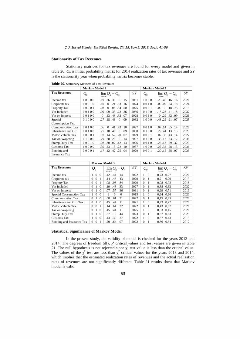
Stationarity of Tax Revenues
Stationary matrices for tax revenues are found for every model and given in
table 20. Q0 is initial probability matrix for 2014 realization rates of tax revenues and SY
is the stationarity year when probability matrix becomes stable.
Table 20. Stationary Matrices of Tax Revenues Markov Model 1 Markov Model 2
Tax Revenues 0Q
QQnnlim SY
0Q
QQn
nlim SY
Income tax 1 0 0 0 0 .19 .36 .30 0 .15 2031 1 0 0 0 .28 .40 .16 .16 2026
Corporate tax 0 0 0 1 0 .10 0 .21 .53 .16 2024 0 0 1 0 .09 .09 .64 .18 2024
Property Tax 0 0 0 0 1 .08 0 .08 .34 .50 2025 0 0 0 1 .09 0 .18 .73 2019
Vat Included 0 0 1 0 0 .09 .09 .35 .22 .26 2036 0 1 0 0 .18 .23 .41 .18 2032
Vat on Imports 0 0 1 0 0 0 .13 .48 .32 .07 2028 0 0 1 0 0 .29 .62 .09 2021
Special
Consumption Tax
0 1 0 0 0 .27 .18 .46 0 .09 2032 1 0 0 0 .43 .29 .21 .07 2025
Communication Tax 0 0 1 0 0 .06 0 .41 .43 .10 2027 0 0 1 0 .07 .14 .65 .14 2026
Inheritence and Gift 0 0 1 0 0 .27 .18 .46 0 .09 2030 0 1 0 0 .29 .44 .13 .13 2023
Motor Vehicle Tax 0 0 0 0 1 .07 .14 .52 .20 .07 2029 0 0 0 1 .07 .36 .43 .14 2027
Tax on Wagering 0 1 0 0 0 .29 .28 .29 0 .14 2097 0 1 0 0 .38 .17 .33 .12 2038
Stamp Duty Tax 0 0 0 1 0 .08 .30 .07 .42 .13 2026 0 0 1 0 .26 .13 .29 .32 2023
Customs Tax 1 0 0 0 0 .30 .23 .15 .22 .10 2037 1 0 0 0 .27 .32 .28 .13 2036
Banking and Insurance Tax
0 0 0 0 1 .17 .12 .42 .25 .04 2029 0 0 0 1 .20 .15 .58 .07 2025
Markov Model 3 Markov Model 4
Tax Revenues 0Q
QQnnlim SY
0Q
QQn
nlim SY
Income tax 1 0 0 .42 .44 .14 2022 1 0 0,73 0,27 2020
Corporate tax 0 0 1 .14 .43 .43 2020 0 1 0,21 0,79 2019
Property Tax 0 0 1 .08 .08 .84 2020 0 1 0,08 0,92 2018
Vat Included 0 1 0 .19 .48 .33 2027 0 1 0,38 0,62 2032
Vat on Imports 0 1 0 .07 .57 .36 2031 0 1 0,29 0,71 2019
Special Consumption Tax 1 0 0 1 0 0 2015 1 0 0,64 0,36 2020
Communication Tax 0 1 0 .08 .61 .31 2022 0 1 0,15 0,85 2023
Inheritence and Gift Tax 0 1 0 .45 .44 .11 2021 1 0 0,73 0,27 2020
Motor Vehicle Tax 0 0 1 .14 .64 .22 2022 0 1 0,43 0,57 2026
Tax on Wagering 0 1 0 .45 .44 .11 2025 1 0 0,53 0,45 2020
Stamp Duty Tax 0 1 0 .37 .19 .44 2023 0 1 0,37 0,63 2023
Customs Tax 1 0 0 .43 .30 .27 2022 1 0 0,57 0,43 2019
Banking and Insurance Tax 0 0 1 .29 .64 .07 2022 0 1 0,36 0,64 2017
Statistical Significance of Markov Model
In the present study, the validity of model is checked for the years 2013 and
2014. The degrees of freedom (df), χ2 critical values and test values are given in table
21. The null hypothesis is not rejected since χ2 test value is less than the critical value.
The values of the χ2 test are less than χ
2 critical values for the years 2013 and 2014,
which implies that the estimated realization rates of revenues and the actual realization
rates of revenues are not significantly different. Table 21 results show that Markov
model is valid.

Ç.Ü. Sosyal Bilimler Enstitüsü Dergisi, Cilt 25, Sayı 2, 2016, Sayfa 41-56
54
Table 21. Validity of Tax Revenues 2013 2014
Tax Revenues df Χ20,05
Crit.V
Χ20,05
Test V
H0:
Valid
df Χ20,05
Crit.V
Χ20,05
Test V
H0:
Valid
Income tax 2 5,991 1,12 Accept 2 5,991 2,03 Accept
Corporate tax 1 3,841 0,17 Accept 2 5,991 4 Accept
Property Tax 2 5,991 0,29 Accept 2 5,991 0,25 Accept
Vat Included 1 3,841 2 Accept 1 3,841 3,5 Accept
Vat on Imports 1 3,841 0,75 Accept 1 3,841 0,75 Accept
Special Consumption Tax 1 3,841 0,67 Accept 1 3,841 0,5 Accept
Communication Tax 2 5,991 1 Accept 2 5,991 0,75 Accept
Inheritence and Gift Tax 1 3,841 0,4 Accept 1 3,841 0,33 Accept
Motor Vehicle Tax 1 3,841 0,5 Accept 1 3,841 0,4 Accept
Tax on Wagering 1 3,841 2 Accept 1 3,841 1 Accept
Stamp Duty Tax 1 3,841 1 Accept 1 3,841 0,5 Accept
Customs Tax 1 3,841 1 Accept 1 3,841 0,5 Accept
Banking and Insurance Tax 1 3,841 0,8 Accept 1 3,841 0,5 Accept
Findings, Discussion and Results
According to transition matrices, transitions of tax revenues are declining in
higher states and improving in lower states. 2016 predictions with respect to middle
state using the better models are given in table 22.
Table 22. Tax Revenue Predictions For 2016 According to Better Models
Tax Revenues
Better
Markov
Model
Realization Rate r
(%)
Predictions For 2016
According to Better Models
Probability
(%)
1 – Probability
(%)
Income tax 1 C or higher 96,7 ≤ r 100 0
Corporate tax 2 C or higher 97,2 ≤ r 76 24
Property Tax 3 B or higher 103,1 ≤ r 14 86
Inheritence and Gift Tax 1 C or higher 91,5 ≤ r 93 7
Motor Vehicle Tax 1 C or higher 100,2 ≤ r 75 25
Vat Included 1 C or higher 101 ≤ r 75 25
Special Consumption Tax 3 B or higher 94,2 ≤ r 80 20
Banking and Insurance Tax 1 C or higher 96,8 ≤ r 80 20
Tax on Wagering 1 C or higher 94,7 ≤ r 100 0
Special Communication Tax 1 C or higher 97,9 ≤ r 42 58
Tax on Customs 1 C or higher 93,1 ≤ r 67 33
Vat on Imports 1 C or higher 99,1 ≤ r 60 40
Stamp Duty Tax 1 C or higher 100,6 ≤ r 36 74
According to model 1 of income tax, the probabilities of five states will be
stable in 2031. Income tax rate more likely will be realized at 102.5% or higher in the
long run. Probability of income tax rate greater than 108.3% is improving from 10% in
2016 to a stable 19.05%. Probability of income tax rate between 102.5% and 108.2% is
improving from 20% in 2016 to a stable 35.71%. Probability of 96.7 ≤ r ≤ 102.4 is
decreasing from 70% to a stable 29.76%. Other tax revenues predictions are compared
in table 23.

Ç.Ü. Sosyal Bilimler Enstitüsü Dergisi, Cilt 25, Sayı 2, 2016, Sayfa 41-56
55
Table 23. Comparison of 2016 Predictions To Stationary Matrices According to Better Models
Tax Revenues
Better
Markov
Model
Comparison of 2016 Predictions To Stationary Matrices
According to Better Models
2016 Prediction Stationary Matrix SY
Income tax 1 .10 .20 .70 0 0 .19 .36 .30 0 .15 2031
Corporate tax 2 .04 .10 .62 .24 .09 .09 .64 .18 2024
Property Tax 3 .07 .07 .86 .08 .08 .84 2020
Inheritence and Gift Tax 1 .29 .15 .49 0 0 .27 .18 .46 0 .09 2030
Motor Vehicle Tax 1 0 .50 .25 .25 0 .07 .14 .52 .20 .07 2029
Vat Included 1 .12 .13 .50 0 .25 .09 .09 .35 .22 .26 2036
Special Consumption Tax 3 .24 .56 .20 1 0 0 2015
Banking and Insurance Tax 1 .20 .20 .40 .20 0 .17 .12 .42 .25 .04 2029
Tax on Wagering 1 .25 0 .75 0 0 .29 .28 .29 0 .14 2097
Special Communication Tax 1 .07 0 .35 .52 .06 .06 0 .41 .43 .10 2027
Tax on Customs 1 .45 .11 .11 .11 .22 .30 .23 .15 .22 .10 2037
Vat on Imports 1 0 0 .60 .32 .08 0 .13 .48 .32 .07 2031
Stamp Duty Tax 1 .08 .23 .05 .46 .18 .08 .30 .07 .42 .13 2026
This study can be used to predict the other sub-items of tax revenues. Central
government can take the advantages of this study in the planning and improvement of
tax collection process.
Resources
Usher M.B, Jun., 1979, Markovian Approaches to Ecological Succession, Journal of
Animal Ecology, 48(2):413-426
Taha H.A, Yöneylem Araştırması, 6.baskıdan çeviri, Literatür Yayıncılık, 2000: 726
Yeh HW, Chan W, Symanski E, Davis B.R, 2010, Estimating Transition Probabilities
for Ignorable Intermittent Missing Data in a Discrete-Time Markov Chain,
Communications in Statistics-Simulation and Computation, 39(2):433-448
Baasch A, Tischew S and Bruelheide H, June 2010, Twelve years of succession on
sandy substrates in a post-mining landscape: A Markov chain analysis,
Ecological Applications, 20(4):1136-1147
Grimshaw S.D, Alexander W.P, 2011, Markov Chain Models for Deliquency:
Transition Matrix Estimation and Forecasting, John Wiley&Sons, Applied
Stochastic Models in Business and Industry, 27: 267-279
Lipták K, 2011, The Application Of Markov Chain Model To The Description Of
Hungarian Labor Market Processes, Zarządzanie Publiczne 4(16):133–149
Büyüktatlı F, İşbilir S, Çetin E.İ, 2013, Markov Analizi ile Yıllık Ödeneklere Bağlı Bir
Tahmin Uygulaması, Uluslararası Alanya İşletme Fakültesi Dergisi (5):1-8
Lukić P.,Gocić M., Trajković S., 2013, Prediction of annual precipitation on the
territory of south Serbia using markov chains, Bulletin of the Faculty of
Forestry, 108: 81-92.

Ç.Ü. Sosyal Bilimler Enstitüsü Dergisi, Cilt 25, Sayı 2, 2016, Sayfa 41-56
56
Bluman A.G, 2014, Elemantary Statistics, McGraw Hill Education, New York
Vantika S., Pasaribu U.S, 2014, Application of Markov Chain To the Pattern of
Mitochondrical Deoxyribonucleic Acid Mutations, AIP Conference Proc. 1589, 296
İlarslan K, 2014, Hisse Senedi Fiyat Hareketlerinin Tahmin Edilmesinde Markov
Zincirlerinin Kullanılması: IMKB 10 Bankacılık Endeksi İşletmeleri Üzerine
Ampirik Bir Çalışma, E-Journal of Yaşar University, 9(35): 6099-6260
Cavers M.S., Vasudevan K., 2015, Brief Communication: Earthquake sequencing:
Analysis of Time Series constructed from the Markov Chain Model, Nonlinear
Process Geophysics, 22:589-599
Lazri M., Ameur S., Brucker J.M., Lahdir M. and Sehad M., Analysis of drought areas
in northern Algeria using Markov chains, February 2015, J. Earth Syst. Sci.
124(1):61–70
http://www.gib.gov.tr/sites/default/files/fileadmin/user_upload/VI/GBG/Tablo_47.xls.ht
m 5.12.2015
http://www.gib.gov.tr/sites/default/files/fileadmin/user_upload/VI/GBG/Tablo_44.xls.ht
m 5.12.2015
http://www.gib.gov.tr/sites/default/files/fileadmin/user_upload/VI/GBG/Tablo_46.xls.ht
m 5.12.2015
http://www.gib.gov.tr/sites/default/files/fileadmin/user_upload/VI/GBG/Tablo_45.xls.ht
m 5.12.2015
www.ekodialog.com>konular>genel_butce 8.12.2015
http://www.hurriyet.com.tr/2016-vergi-artis-oranlari-belli-oldu-40009417 9.12.2016
http://www.zaman.com.tr/ekonomi_2015-yilinda-vergiler-yuzde-1011-oraninda-
artacak_2255169.html 10.12.2015
galton.uchicago.edu/~lalley/Courses/312/MarkovChains.pdf 15.12.2015
dept.stat.lsa.umich.edu/~ionides/620/notes/markov_chains.pdf 15.12.2015


