HAL Id: hal-00872639https://hal.archives-ouvertes.fr/hal-00872639

Submitted on 14 Oct 2013

HAL is a multi-disciplinary open accessarchive for the deposit and dissemination of sci-entific research documents, whether they are pub-lished or not. The documents may come fromteaching and research institutions in France orabroad, or from public or private research centers.

L’archive ouverte pluridisciplinaire HAL, estdestinée au dépôt et à la diffusion de documentsscientifiques de niveau recherche, publiés ou non,émanant des établissements d’enseignement et derecherche français ou étrangers, des laboratoirespublics ou privés.

Prediction of Solid Polycyclic Aromatic HydrocarbonsSolubility in Water with the NRTL-PR Model

Joan Escandell, Isabelle Raspo, Evelyne Neau

To cite this version:Joan Escandell, Isabelle Raspo, Evelyne Neau. Prediction of Solid Polycyclic Aromatic HydrocarbonsSolubility in Water with the NRTL-PR Model. Fluid Phase Equilibria, Elsevier, 2014, 362 (25),pp.87-95. <10.1016/j.fluid.2013.09.009>. <hal-00872639>

Prediction of Solid Polycyclic Aromatic Hydrocarbons Solubility in Water

with the NRTL-PR Model

Joan Escandella, Isabelle Raspo

b, Evelyne Neau

a

aAix-Marseille Universite, CNRS, Centrale Marseille, M2P2 UMR 7340, Faculty of Sciences of Luminy, 13288 Marseille, France bAix-Marseille Universite, CNRS, Centrale Marseille, M2P2 UMR 7340, Technopôle de Château-Gombert, 13451 Marseille, France

Abstract

The accurate prediction of high pressure phase equilibria is crucial for the development and the

design of chemical engineering processes. Among them the modeling of complex systems, such as

petroleum fluids with water, has become more and more important with the exploitation of reservoirs

in extreme conditions. The aim of this work is to explore the capability of the NRTL-PR model to

predict the solubility of solid polycyclic aromatic hydrocarbons in water. For this purpose, we first

validate our methodology for fluid phase equilibria predictions of aromatic hydrocarbons and gas

(CO2, C2H6) mixtures. Finally, we consider the prediction of the solid solubility of PAH in water, by

fitting group parameters either only on SLE data or on both LLE and SLE data of aromatic

hydrocarbon-water binary systems.

Keywords: solubility; solid-liquid equilibrium; EoS/GE approach; NRTL-PR model; polycyclic

aromatic hydrocarbons; water.

1. Introduction

Polycyclic aromatic hydrocarbons (PAH) are very toxic substances which are often generated by

human activities. They can be found in hydrocarbon-contaminated waste sites or in the sea after oil

discharges by ships. They are also produced by offshore oil and gas exploration [1] and by several

combustion processes [2,3], among others. Because these pollutants accumulate in soils and

sediments and are persistent in the environment, it is crucial to understand their transport and

transformation processes [4]. The solubility in water is an important transport property in the

potential distribution of these compounds throughout the hydrologic system. Besides, the solubility is

also necessary for the design of extraction processes of PAH with subcritical water [5,6] since it

provides the extractability limit which can be used. Therefore, a good representation of solid-liquid

equilibria in water-PAH mixtures is essential for many practical applications; but PAH are highly

hydrophobic compounds and, consequently, an accurate prediction of their very low solubilities is

difficult to obtain.

In literature, models proposed for the calculation of non-polar hydrophobic compound aqueous

solubility are essentially based on empirical or semi-empirical equations, which do not allow

accurate results at both low and high temperatures [7]. However, for some years, a few papers were

concerned with the modeling of solid-liquid equilibria in water-PAH systems by means of equations

of state and GE models. Fornari et al. [8] compared the accuracy of the original UNIFAC, the

modified version of Dortmund and the A-UNIFAC models, the latter including association effects

between groups, for the representation of the solubility of solid PAH in subcritical water. These

authors showed that the modified UNIFAC model gives a better prediction than the A-UNIFAC one,

provided that the interaction parameters between water and aromatic groups are optimized by taking

into account SLE data in the parameter fitting procedure. More recently, the CPA EoS, which adds

an association term to the SRK equation of state, was applied by Oliveira et al. [9] to the modeling of

the aqueous solubility of PAH. The major advantage of EoS based models, such as CPA, compared

to GE models, such as UNIFAC, is to allow solubility predictions in a wide range of temperature and

pressure, and especially under high pressures. Oliveira et al. showed that a good representation of the

solubility of PAH can be obtained by fitting the solvation parameter for each binary water-PAH

system on SLE data.

The purpose of this work is to explore the capability of the NRTL-PR model [10,11] to predict

solid-liquid equilibria (SLE) in water-PAH mixtures. This model is based on the EoS/GE approach in

which the Peng-Robinson equation of state is associated with the generalized NRTL excess Gibbs

energy model [12]. In this formalism, binary interaction parameters are estimated from group

contributions providing a totally predictive EoS. In order to validate the approach, the NRTL-PR

model is first applied to the prediction of vapor-liquid equilibria (VLE) and of the solid solubility in

supercritical fluids (SFE) of aromatic hydrocarbons with carbon dioxide or ethane. Then we

investigate the capability of the model to predict both liquid-liquid equilibria (LLE) of aromatic

hydrocarbons in water and the very low solubilities of PAH (SLE).

2. Modeling

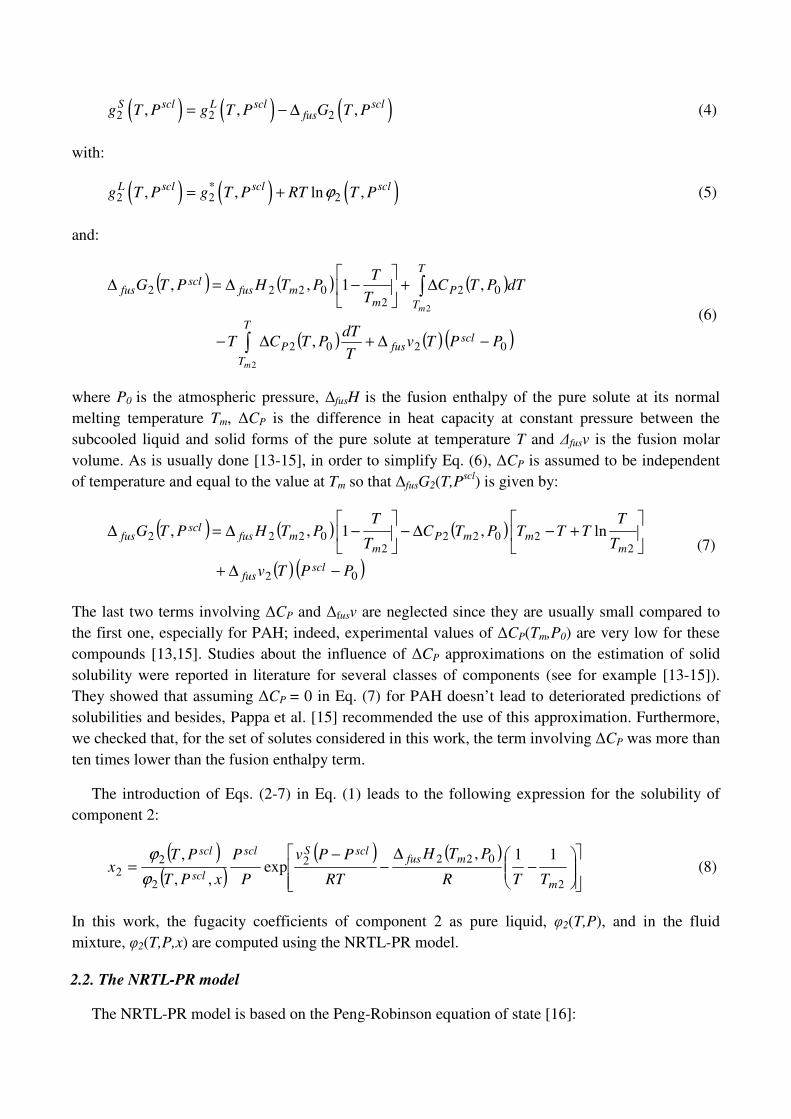
2.1. Solid-fluid equilibrium

Solid-fluid equilibrium of binary mixtures of solvent(1)-PAH(2) is described assuming that the

solid phase is pure PAH(2). The equilibrium condition for this component is thus written as:

( ) ( )2 2, , ,S Fg T P g T P x= (1)

where ( )2 ,Sg T P and ( )2 , ,F

g T P x are the molar Gibbs free energies of the pure solid (2) and of the

solute in the fluid mixture, under the same temperature and pressure conditions; they are calculated

by the following equations:

( ) ( ) ( )2 2 2, ,= + −S S ref S refg T P g T P v P P (2)

( ) ( ) ( )*2 2 2 2, , , ln , ,F ref

ref

Pg T P x g T P RT T P x x

Pϕ

= + (3)

with: Pref

a reference pressure, 2S

v the molar volume of the solid, ( )*2 , ref

g T P the Gibbs free energy

of pure compound 2 in the standard state and φ2(T,P,x) the fugacity coefficient in the fluid phase.

The subcooled liquid pressure, Pscl

, is chosen as the reference pressure, so that the term ( )2 ,S refg T P

in Eq. (2) can be obtained from the Gibbs free energy of 2 as pure liquid, ( )2 ,L sclg T P , considering

the fusion properties:

( ) ( ) ( )2 2 2, , ,S scl L scl sclfusg T P g T P G T P= − ∆ (4)

with:

( ) ( ) ( )*2 2 2, , ln ,L scl scl scl

g T P g T P RT T Pϕ= + (5)

and:

( ) ( ) ( )

( ) ( ) ( )0202

022

0222

,

,1 ,,

2

2

PPTvT

dTPTCT

dTPTCT

TPTHPTG

sclT

T

fusP

T

T

Pm

mfusscl

fus

m

m

−∆+∆−

∆+

−∆=∆

∫

∫ (6)

where P0 is the atmospheric pressure, ∆fusH is the fusion enthalpy of the pure solute at its normal

melting temperature Tm, ∆CP is the difference in heat capacity at constant pressure between the

subcooled liquid and solid forms of the pure solute at temperature T and ∆fusv is the fusion molar

volume. As is usually done [13-15], in order to simplify Eq. (6), ∆CP is assumed to be independent

of temperature and equal to the value at Tm so that ∆fusG2(T,Pscl

) is given by:

( ) ( ) ( )

( ) ( )02

22022

20222

ln , 1 ,,

PPTv

T

TTTTPTC

T

TPTHPTG

sclfus

mmmP

mmfus

sclfus

−∆+

+−∆−

−∆=∆

(7)

The last two terms involving ∆CP and ∆fusv are neglected since they are usually small compared to

the first one, especially for PAH; indeed, experimental values of ∆CP(Tm,P0) are very low for these

compounds [13,15]. Studies about the influence of ∆CP approximations on the estimation of solid

solubility were reported in literature for several classes of components (see for example [13-15]).

They showed that assuming ∆CP = 0 in Eq. (7) for PAH doesn’t lead to deteriorated predictions of

solubilities and besides, Pappa et al. [15] recommended the use of this approximation. Furthermore,

we checked that, for the set of solutes considered in this work, the term involving ∆CP was more than

ten times lower than the fusion enthalpy term.

The introduction of Eqs. (2-7) in Eq. (1) leads to the following expression for the solubility of

component 2:

( )( )

( ) ( )

−

∆−

−=

2

0222

2

22

11,exp

,,

,

m

mfussclSscl

scl

scl

TTR

PTH

RT

PPv

P

P

xPT

PTx

ϕ

ϕ (8)

In this work, the fugacity coefficients of component 2 as pure liquid, φ2(T,P), and in the fluid

mixture, φ2(T,P,x) are computed using the NRTL-PR model.

2.2. The NRTL-PR model

The NRTL-PR model is based on the Peng-Robinson equation of state [16]:

2 22

RT aP

v b v bv b= −

− + − (9)

in which the attractive term a is estimated using the EoS/GE approach based on the generalized

reference state proposed in [17]:

1ln

0.53

Ei

i i ii i

a g rx x

bRT RT rα α

= = − −

∑ ∑ (10)

where b is the covolume, i iib x b=∑ , ri and i ii

r x r=∑ are the volume area factors characteristic of

lattice fluid models and gE is the excess Gibbs energy expressed, with the generalized NRTL

equation [12], as:

ln

j j ji jijE i

i i il l lii i

l

x q Gr

g RT x x qr x q G

Γ

= +

∑∑ ∑

∑ , ( )0expji jiG RTα Γ= − (11)

So that:

1

0.53

Eres

i ii

gx

RTα α

= −

∑ ,

j j ji jijE

res i il l lii

l

x q G

g x qx q G

Γ

=

∑∑

∑ (12)

In the above equation, α0 is the non randomness factor (α0 = -1) and qi are the lattice fluid surface

area parameters, estimated from the UNIFAC subgroups Qk:

i ik kk

q Qν=∑ (13)

with νik the number of subgroup k in a molecule i. The group contribution and the surface area

parameters Qk considered in the NRTL-PR model are indicated in Table 1. It must be noted that no

distinction is made between substituted single benzene ring carbons and fused-ring carbons. In Eqs.

(11-12) the binary interaction parameters Γji are computed by means of a group contribution [10]

which makes the NRTL-PR equation a totally predictive model:

( ) ( ) , kji iK jL iL LK iK ik K

iK L k

Q

qΓ θ θ θ Γ θ ν= − =∑ ∑ ∑ with : 0 , KK KL LKΓ Γ Γ= ≠ (14)

where θiK is the probability that a contact from a molecule i involves a main group K and νik(K) is the

number of subgroup k belonging to the main group K in a molecule i. The group interaction

parameters ΓLK depend on temperature with the following equation:

(0) (1) 001 with 298.15KLK LK LK

TT

TΓ Γ Γ

= + − =

(15)

Finally, the model requires the estimation of pure component parameters: the attractive term ai and

the covolume bi (necessary to calculate αi in Eq. (12)) are estimated from the critical temperature and

pressure, Tci and Pci respectively, by the formulae:

( )2 2

0.4572 , 0.0778i i

i i

c ci r i

c c

R T RTa f T b

P P= = (16)

where Tr is the reduced temperature, ir cT T T= , and f(Tr) is the generalized Soave function [20]:

( ) ( )2

1 1r rf T m T γ = + −

(17)

For hydrocarbons and non associating compounds, we used the original Soave function [21],

corresponding to γ = 0.5, and the parameter m correlated to the acentric factor ω through the

generalized expression proposed by Robinson and Peng [22]:

2

2 3

0.37464 1.54226 0.26992 if 0.49

0.379642 1.48503 0.164423 +0.016666 if 0.49

m

m

ω ω ω

ω ω ω ω

= + − <

= + − ≥ (18)

On the other hand, for associating compounds, the γ and m parameters were fitted on saturation

properties as proposed in [20], which allows highly improved vapor pressure representations. For

water the fitted values are : γ = 0.65, m = 0.6864.

With the NRTL-PR equation, the fugacity coefficient of a component i is given by the following

relation:

( ) ( )( )( ) ,

1 1 21 1ln ln 1 1 ln

2 2 1 1 2j j

ii in T n

nb nZ Z

b n n

η αϕ η

η

+ + ∂ ∂ = − − + − − ∂ ∂ + −

(19)

where Z is the compressibility factor, η = b/v and :

, ,

1

0.53j j

Ei res

i i iT n T n

n a ng

n b RT n

α ∂ ∂= − ∂ ∂

(20)

3. Results

The set of solvents and PAH considered in this work is given in Table 2, together with the values

of the pure component properties. For PAH, the normal melting temperatures, Tm, and fusion

enthalpies at melting point, ∆fusH, as well as the solid volumes, v2s, were taken from literature.

3.1. Solubility of PAH in supercritical fluids

As already mentioned in the introduction, PAH are highly hydrophobic compounds. Therefore, an

accurate representation of their very low solubilities in water is very difficult to obtain. As a

consequence, water-PAH systems are not the most appropriate to check if a model is able to predict

correctly solid-fluid equilibria. Thus, in order to validate the approach proposed in section 2, we first

considered the solubility of PAH in supercritical fluids; indeed, as can be seen in Tables 3 and 4 for

CO2 and ethane, the experimental values are about three orders of magnitude higher than those in

liquid water.

The calculation of solid-fluid equilibria of CO2-PAH and ethane-PAH mixtures with the NRTL-

PR model (Eq. 12) requires fitting the EoS binary parameters Γaromatic,CO2 and Γaromatic,C2H6 (Eqs. 14,

15) taking into account simultaneously VLE and SFE data. Results thus obtained on PAH solubilities

in supercritical carbon dioxide and ethane are reported respectively in Tables 3 and 4. For almost all

mixtures, mean deviations are smaller than 30%, except for some heavier compounds involving at

least three benzene rings and exhibiting lower solubilities.

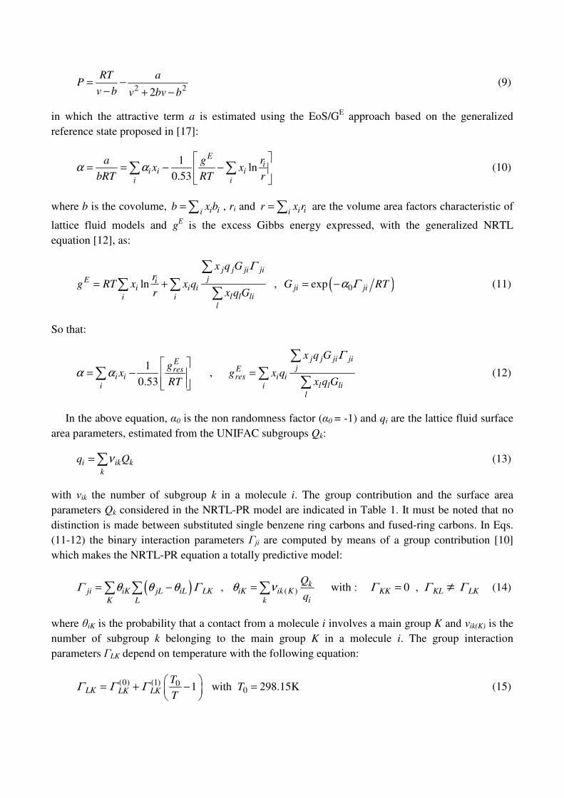
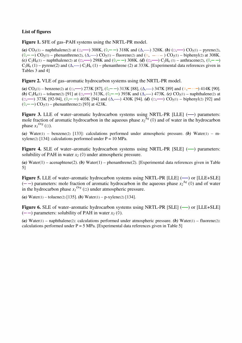
Figure 1 illustrates the prediction of solubilities, with respect to pressure, for the most

representative systems in the range of experimental temperature. It can be seen that for mixtures of

naphthalene, pyrene, phenanthrene, fluorene and biphenyl with CO2, as well as naphthalene with

ethane, predictions with the NRTL-PR model are in very good agreement with experimental data.

Figure 1d, concerning anthracene, pyrene and phenanthrene with supercritical ethane, shows that,

despite higher deviations, a satisfactory representation of the solubilities is obtained. For

measurements made in the vicinity of the mixture lower critical endpoint (Fig. 1a), the strong

variation of the solubility with respect to pressure and the retrograde solubility phenomenon are

accurately described.

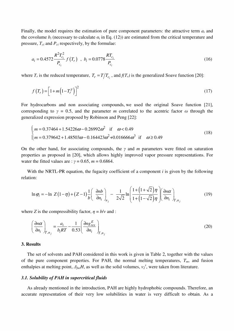
To ensure that VLE predictions were not deteriorated by considering SFE data during parameter

fitting procedure, we represent in Fig. 2 VLE for aromatic hydrocarbons. Figures 2a and 2b for CO2-

benzene and ethane-toluene highlight that results are similar to those previously published [11] for

single benzene ring molecules. Furthermore, as shown in Figs. 2c and 2d, satisfactory phase

envelopes are calculated for gas-PAH systems, although experimental data are not available in the

whole composition range.

We can therefore conclude that the NRTL-PR model is able to accurately estimate VLE of

aromatic hydrocarbons and solubilities of PAH in solvents with the same set of parameters.

3.2. Application to the solubility of PAH in liquid water

The calculation of SLE of water-PAH mixtures with the NRTL-PR model (Eq. 12) also requires

the values of the EoS binary parameters Γ aromatic,H2O and ΓH2O,aromatic (Eqs. 14, 15).

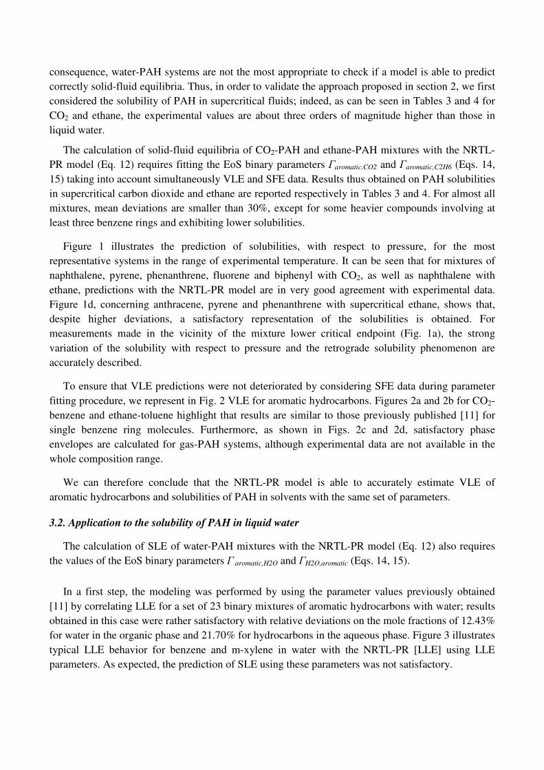
In a first step, the modeling was performed by using the parameter values previously obtained

[11] by correlating LLE for a set of 23 binary mixtures of aromatic hydrocarbons with water; results

obtained in this case were rather satisfactory with relative deviations on the mole fractions of 12.43%

for water in the organic phase and 21.70% for hydrocarbons in the aqueous phase. Figure 3 illustrates

typical LLE behavior for benzene and m-xylene in water with the NRTL-PR [LLE] using LLE

parameters. As expected, the prediction of SLE using these parameters was not satisfactory.

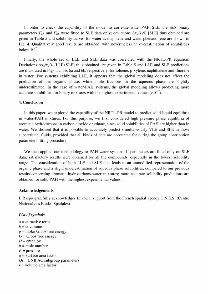
In order to check the capability of the model to correlate water-PAH SLE, the EoS binary

parameters ΓLK and ΓKL were fitted to SLE data only; deviations ∆x2/x2% [SLE] thus obtained are

given in Table 5 and solubility curves for water-acenaphtene and water-phenanthrene are shown in

Fig. 4. Qualitatively good results are obtained, with nevertheless an overestimation of solubilities

below 10-7

.

Finally, the whole set of LLE and SLE data was correlated with the NRTL-PR equation.

Deviations ∆x2/x2% [LLE+SLE] thus obtained are given in Table 5 and LLE and SLE predictions

are illustrated in Figs. 5a, 5b, 6a and 6b, respectively, for toluene, p-xylene, naphthalene and fluorene

in water. For systems exhibiting LLE, it appears that the global modeling does not affect the

prediction of the organic phase, while mole fractions in the aqueous phase are slightly

underestimated. In the case of water-PAH systems, the global modeling allows predicting more

accurate solubilities for binary mixtures with the highest experimental values (>10-7

).

4. Conclusion

In this paper, we explored the capability of the NRTL-PR model to predict solid-liquid equilibria

in water-PAH mixtures. For this purpose, we first considered high pressure phase equilibria of

aromatic hydrocarbons in carbon dioxide or ethane, since solid solubilities of PAH are higher than in

water. We showed that it is possible to accurately predict simultaneously VLE and SFE in those

supercritical fluids, provided that all kinds of data are accounted for during the group contribution

parameters fitting procedure.

We then applied our methodology to PAH-water systems. If parameters are fitted only on SLE

data, satisfactory results were obtained for all the compounds, especially in the lowest solubility

range. The consideration of both LLE and SLE data leads to an unmodified representation of the

organic phase and a slight underestimation of aqueous phase solubilities, compared to our previous

results concerning aromatic hydrocarbons-water mixtures; more accurate solubility predictions are

obtained for solid PAH with the highest experimental values.

Acknowledgements

I. Raspo gratefully acknowledges financial support from the French spatial agency C.N.E.S. (Centre

National des Etudes Spatiales).

List of symbols

a = attractive term

b = covolume

g = molar Gibbs free energy

G = Gibbs free energy

H = enthalpy

n = mole number

P = pressure

q = surface area factor

Qk = UNIFAC subgroup parameters

r = volume area factor

R = ideal gas constant

T = temperature

v = molar volume

x = mole fraction

Z = compressibility factor

Greek letters

α = alpha function

α0 = non randomness factor

η = packing fraction

φ = fugacity coefficient

Γji = interaction parameter between molecules j and i

ΓLK(0)

, ΓLK(1)

= interaction parameters between main groups K and L

ω = acentric factor

θiK = probability that a contact from molecule i involves a main group K

νiK = number of main group K in a molecule i

Subscript

c = critical property

fus = fusion property

i = pure component property

res = residual property

Superscript

E = excess property at constant pressure

F = fluid phase

L = liquid state

ref = reference property

S = solid state

scl = subcooled liquid

References

[1] P.G. Wells, Mar. Pollut. Bull. 42 (2001) 251-252.

[2] S.K.Durlak, P.Biswas, J.Shi, M.J. Bernhard, Environ. Sci. Technol. 32 (1998) 2301-2307.

[3] J.J. Schauer, M.J.Kleeman, G.R.Cass, B.R.T.Simoneit, Environ. Sci. Technol. 35 (2001) 1716-

1728.

[4] M.G. Zemanek, J.T.S. Pollard, S.L. Kenefick, S.E.Hrudey, Environ. Pollut. 98 (1997) 239-252.

[5] S.B. Hawthorne, Y. Yang, D.J. Miller, Anal. Chem. 66 (1994) 2912-1920.

[6] Y. Yang, S.B. Hawthorne, D.J. Miller, Environ. Sci. Technol. 31 (1997) 430-437.

[7] A.G. Carr, R. Mammucari, N.R. Foster, Chem. Eng. J. 172 (2011) 1-17.

[8] T. Fornari, R.P. Stateva, F.J. Señorans, G. Reglero, E. Ibañez, J. Super. Fluids. 46 (2008) 245-

251.

[9] M.B. Oliveira, V.L. Oliveira, J.A.P. Coutinho, A.J. Queimada, Ind. Eng. Chem. Res. 48 (2009)

5530-5536.

[10] E. Neau, J. Escandell, C. Nicolas, Ind. Eng. Chem. Res. 49 (2010) 7589-7596.

[11] J. Escandell, E. Neau, C. Nicolas, Fluid Phase Equilib. 301 (2011) 80-97.

[12] E. Neau, J. Escandell, C. Nicolas, Ind. Eng. Chem. Res. 49 (2010) 7580-7588.

[13] S.H. Neau, G.L. Flynn, Pharm. Res. 7 (1990) 1157-1162.

[14] D.S. Mishra, S.H. Yalkowsky, Pharm. Res. 9 (1992) 958-959.

[15] G.D. Pappa, E.C. Voutsas, K. Magoulas, D.P. Tassios, Ind. Eng. Chem. Res., 44 (2005) 3799-

3806.

[16] D.Y. Peng, D.B. Robinson, Ind. Chem. Fundam. 15 (1976) 59-64.

[17] E. Neau, J. Escandell, I. Raspo, Chem. Eng. Sci. 66 (2011), 4148-4156.

[18] A. Fredenslund, J. Gmehling, P. Rasmusen, Vapor-Liquid equilibrium using UNIFAC, Elsevier,

Amsterdam, 1977.

[19] T. Holderbaum, J. Gmehling, Fluid Phase Equilib. 70 (1991) 251-265.

[20] E. Neau, I. Raspo, J. Escandell, C. Nicolas, O. Hernández-Garduza, Fluid Phase Equilib. 276

(2009), 156-164.

[21] G. Soave, Chem. Eng. Sci. 27 (1972) 1197-1340.

[22] D.B. Robinson, D.Y. Peng, RR-28 The Characterization of the Heptanes and Heavier Fractions

for the GPA Peng-Robinson Programs, Gas Processors Association Research Report, Edmonton-

Alberta, 1978.

[23] S. Angus, B. Armstrong, K.M. de Reuck, International Thermodynamics Tables of the Fluid

State Carbon Dioxide, Pergamon Press, Oxford, 1976.

[24] B.E. Poling, J.M. Prausnitz, J.P. O’Connell, The properties of Gases and Liquids, 5th

ed.,

McGraw-Hill, New York, 2004.

[25] R.D. Goodwin, Provisional Values for the Thermodynamic Functions of Ethane, American Gas

Association, Research Report NBSIR 74-398, 1974.

[26] M. Skerget, Z. Novak-Pintaric, Z. Knez, Z. Kravanja, Fluid Phase Equilib. 203 (2002) 111-132.

[27] L. Constantinou, R. Gani, J.P. O’Connell, Fluid Phase Equilib. 103 (1995) 11-22.

[28] A.M. Chaudhury, Current Sci. 24 (1955) 80-81.

[29] R.C. Reid, J.M. Prausnitz, B.E. Poling, The properties of Gases and Liquids, 4th

ed., McGraw-

Hill, New York, 1987.

[30] R.R. Dreisbach, Physical Properties of Chemical Compounds, Advances in Chemistry Series,

ACS Publications, 1961.

[31] C. Nicolas, E. Neau, S. Meradji, I. Raspo, Fluid Phase Equilib. 232 (2005) 219-229.

[32] P. Karasek, J. Planeta, M. Roth, J. Chem. Eng. Data 51 (2006) 616-622.

[33] M. Prasad, L.A. de Sousa, Current Sci. 6 (1937) 220-221.

[34] L. D. Gluzman, A. G. Nikitenko, Zh. Prikl. Khim. (St-Peterburg) 34 (1961) 626-628.

[35] S.T. Chung, K.S. Shing, Fluid Phase Equilib. 81 (1992) 321-341.

[36] M. McHugh, M.E. Paulaitis, J. Chem. Eng. Data 25 (1980) 326-329.

[37] M.E. Paulaitis, M. McHugh, C.P. Chai, Chem. Eng. Super. Fluid Cond. (1983) 139-158.

[38] Z. Suoqi, W. Renan, Y. Guanghua, J. Super. Fluids 8 (1995) 15-19.

[39] K.P. Johnston, D.H. Ziger, C.A. Eckert, Ind. Eng. Chem. Fundam. 21 (1982) 191-197.

[40] A.P. Abbott, S. Corr, N.E. Durling, E.G. Hope, J. Chem. Eng. Data 47 (2002) 900-905.

[41] H.-J. Chang, D.G. Morrell, J. Chem. Eng. Data 30 (1985) 74-78.

[42] J.-W. Chen, F.-N. Tsai, Fluid Phase Equilib. 107 (1995) 189-200.

[43] J.M. Dobbs, J.M. Wong, K.P. Johnston, J. Chem. Eng. Data 31 (1986) 303-308.

[44] J. Garcia-Gonzalez, M.J. Molina, F. Rodriguez, F. Mirada, J. Chem. Eng. Data 46 (2001) 918-

921.

[45] I. Goodarznia, F. Esmaeilzadeh, J. Chem. Eng. Data 47 (2002) 333-338.

[46] A. Kalaga, M. Trebble, J. Chem. Eng. Data 44 (1999) 1063-1066.

[47] R.T. Kurnik, S.J. Holla, R.C. Reid, J. Chem. Eng. Data 26 (1981) 47-51.

[48] L.-S. Lee, J.-H. Fu, H.-L. Hsu, J. Chem. Eng. Data 45 (2000) 358-361.

[49] G.-T. Liu, K. Nagahama, J. Super. Fluids 9 (1996) 152-160.

[50] S. Mitra, J.W. Chen, D.S. Viswanath, J. Chem. Eng. Data 33 (1988) 35-37.

[51] E. Reverchon, P. Russo, A. Stassi, J. Chem. Eng. Data 38 (1993) 458-460.

[52] S. Sako, K. Ohgaki, T. Katayama, J. Super. Fluids 1 (1988) 1-6.

[53] M. Sauceau, J. Fages, J.-J. Letourneau, D. Richon, Ind. Eng. Chem. Res. 39 (2000) 4609-4614.

[54] A. Stassi, R. Bettini, A. Gazzaniga, F. Giordano, A. Schiraldi, J. Chem. Eng. Data 45 (2000)

161-165.

[55] Y.V. Tsekhanskaya, M.B. Iomtev, E.V. Mushkina, Russ. J. Phys. Chem. 38 (1964) 1173-1176.

[56] Y.V. Tsekhanskaya, N.G. Roginskaya, E.V. Musshkina, Russ. J. Phys. Chem. 40 (1966) 1152-

1156.

[57] A. Zuniga-Moreno, L.A. Galicia-Luna, L.E. Camacho-Camacho, Fluid Phase Equilib. 234

(2005) 151-163.

[58] F. Dongbao, S. Xuewen, Q. Yanhua, J. Xiaohui, Z. Suoqi, Fluid Phase Equilib. 251 (2007) 114-

120.

[59] K. Khimeche, P. Alessi, I. Kikic, A. Dahmani, J. Supercrit. Fluids 41 (2007) 10-19.

[60] A. Diefenbacher, M. Turk, J. Supercrit. Fluids 22 (2002) 175-184.

[61] V. Pauchon, Z. Cisse, M. Chavret, J. Jose, J. of Supercritical Fluids 32 (2004) 115-121.

[62] R. Qilong, S. Baogen, H. Mei, W. Pingdong, J. Chem. Eng. Data 45 (2000) 464-466.

[63] W. Jingdai, C. Jizhong, Y. Yongrong, Fluid Phase Equilib. 220 (2004) 147-151.

[64] M. Sahihi, H.S. Ghaziaskar, M. Hajebrahimi, J. Chem. Eng. Data 55 (2010) 2596-2599.

[65] Y. Yamini, R.M. Fat’hi, N. Alizadeh, M. Shamsipur, Fluid Phase Equilib. 152 (1998) 299-305.

[66] H. Buxing, P. Ding-Yu, F. Cheng-Tze, G. Vilcsak, Can. J. Chem. Eng. 70 (1992) 1164-1171.

[67] D.M. Lamb, T.M. Barbara, J. Jonas, J. Phys. Chem. 90 (1986) 4210-4215.

[68] G. Madras, C. Erkey, A. Akgermann, J. Chem. Eng. Data 38 (1993) 422-423.

[69] I. Moradinia, A.S. Teja, Fluid Phase Equilib. 28 (1986) 199-209.

[70] Y. Iwai, Y. Mori, N. Hosotani, H. Higashi, T. Furuya, Y. Arai, K. Yamamoto, Y. Mito, J. Chem.

Eng. data. 38 (1993) 509-511.

[71] G. Anitescu, L.L. Tavlarides, J. Super. Fluids 10 (1997) 175-189.

[72] J.M. Dobbs, K.P. Johnston, Ind. Eng. Chem. Res. 26 (1987) 1476-1482.

[73] F. Esmaeilzadeh, I. Goodarznia, J. Chem. Eng. Data 50 (2005) 49-51.

[74] J.W. Hampson, J. Chem. Eng Data 41 (1996) 97-100.

[75] E. Kosal, G.D. Holder, J. Chem. Eng. Data 32 (1987) 148-150.

[76] J. Kwiatkowski, Z. Lisicki, W. Majewski, Ber. Bunsenges. Phys. Chem. 88 (1984) 865-869.

[77] L. Qunsheng, Z. Zeting, Z. Chongli, L. Yancheng, Z. Qingrong, Fluid Phase Equilib. 207 (2003)

183-192.

[78] T.W. Zerda, B. Wiegand, J. Jonas, J. Chem. Eng. Data 31 (1986) 274-277.

[79] L. Barna, J.-M. Blanchard, E. Rauzy, C. Berro, J. Chem. Eng. Data 41 (1996) 1466-1469.

[80] K.D. Bartle, A.A. Clifford, S.A. Jafar, J. Chem. Eng. Data 35 (1990) 355-360.

[81] L.-S. Lee, J.-F. Huang, O.-X. Zhu, J. Chem. Eng. Data 46 (2001) 1156-1159.

[82] Y. Yamini, N. Bahramifar, J. Chem. Eng. Data 45 (2000) 53-56.

[83] T. Pang, E. McLaughlin, Ind. Eng. Chem. Proc. Des. Dev. 24 (1985) 1027-1032.

[84] K.D. Bartle, J. Chem. Eng. Data 35 (1990) 355-360.

[85] D.J. Miller, S.B. Hawthorne, A.A. Clifford, S. Zhu, J. Chem. Eng. Data 41 (1996) 779-786.

[86] W.J. Schmitt, R.C. Reid, J. Chem. Eng. Data 31 (1986) 204-212.

[87] G.I. Kaminishi, C. Yokoyama, S. Takahashi, Fluid Phase Equilib. 34 (1987) 83-99.

[88] M.K. Gupta, Y.-H. Li, B.J. Hulsey, R.L. Robinson Jr., J. Chem. Eng. Data 27 (1982) 55-57.

[89] P.G. Bendale, R.M. Enick, Fluid Phase Equilib., 94 (1994) 227-253.

[90] H. Inomata, K. Arai, S. Saito, Fluid Phase Equilib. 29 (1986) 225-232.

[91] S. Laugier, A. Valtz, A. Chareton, D. Richon, H. Renon, RR-82 Vapor-Liquid Equilibria

Measurements on the Systems Ethane-Tolune, Ethane-N-Propylbenzene, Ethane-Metaxylene,

Ethane-Mesitylene, Ethane-Methylcyclohexane, Gas Processors Association Research Report,

Edmonton-Alberta, 1984.

[92] D.S. Jan, F.N. Tsai, Ind. Eng. Chem. Res. 30 (1991) 1965-1970.

[93] M.W. Barrick, A.J. McRay, R.L. Robinson Jr., J. Chem. Eng. Data 32 (1987) 372-374.

[94] R.A. Harris, M. Wilken, K. Fischer, T.M. Letcher, J.D. Raal, D. Ramjugernath, Fluid Phase

Equilib. 260 (2007) 60-64.

[95] M. Akiyoshi, T. Deguchi, I. Sanemasa, Bull. Chem. Soc. Jpn. 60 (1987) 3935-3939.

[96] L.J. Andrews, R.M. Keefer, J. Am. Chem. Soc. 71 (1949) 3644-3647.

[97] S. Banerjee, S.H. Yalkowsky, S.C. Valvani, Environ. Sci. Technol. 14 (1980) 1227-1229.

[98] R.L. Bohon, W.F. Claussen, J. Am. Chem. Soc. 73 (1951) 1571-1578.

[99] G.T. Coyle, T.C. Harmon, I.H. Suffet, Environ. Sci. Technol. 31 (1997) 384-389.

[100] R.P. Eganhouse, J.A. Calder, Geochim. Cosmochim. Acta 40 (1976) 555-561.

[101] M. Janado, Y. Yano, Y. Doi, H. Sakamoto, J. Solution Chem. 12 (1983) 741-754.

[102] D. Mackay, W.Y. Shiu, J. Chem. Eng. Data. 22 (1977) 399-402.

[103] M.M. Miller, S. Ghobdane, S.P. Wasik, Y.B. Tewari, D.E. Martire, J. Chem. Eng. Data 29

(1984) 184-190.

[104] A. Vesala, Acta Chem. Scand. Ser. A 28 (1974) 839-845.

[105] R.D. Wauchope, F.W. Getzen, J. Chem. Eng. Data 17 (1972) 38-41

[106] S. Sawamura, M. Tsuchiya, T. Ishigami, Y. Taniguchi, K. Suzuki, J. Solution Chem. 22 (1993)

727-732.

[107] D. Bennett, W.J. Canady, J. Am. Chem. Soc. 106 (1984) 910-915.

[108] R.M. Dickhut, A.W. Andren, D.E. Armstrong, J. Chem. Eng. Data 34 (1989) 438-443.

[109] J.E. Gordon, R.L. Thorne, J. Phys. Chem. 71 (1967) 4390-4399.

[110] S. Hilpert, Angew. Chem. 29 (1916) 57-59.

[111] H.B. Klevens, J. Phys. Chem. 54 (1950) 283-298.

[112] W.E. May, S.P. Wasik, D.H. Freeman, Anal. Chem. 50 (1978) 997-1000.

[113] W.E. May, S.P. Wasik, M.M. Miler, Y.B. Tewari, J.M. Brown-Thomas, J. Chem. Eng. Data 28

(1983) 197-200.

[114] D.J. Miller, S.B. Hawthorne, Anal. Chem. 70 (1998) 1618-1621.

[115] S. Mitchell, J. Chem. Soc. (1926) 1333-1336.

[116] F.P. Schwarz, S.P. Wasik, Anal. Chem. 48 (1976) 524-528.

[117] F.P. Schwarz, S.P. Wasik, J. Chem. Eng. Data 22 (1977) 270-273.

[118] F.P. Schwarz, J. Chem. Eng. Data 22 (1977) 273-277.

[119] F.M. Van Meter, H.M. Neumann, J. Am. Chem. Soc. 98 (1976) 1382-1388.

[120] A. Vesala, H. Lonnberg, Acta Chem. Scand. Ser. A 34 (1980) 187-192.

[121] D.J. Miller, S.B. Hawthorne, A.M. Gizir, A.A. Clifford, J. Chem. Eng. Data 43 (1998) 1043-

1047.

[122] S. Sawamura, J. Solution Chem. 29 (2000) 369-375.

[123] T.A. Andersson, K.M. Hartonen, M-L. Riekkola, J. Chem. Eng. Data 50 (2005) 1177-1783.

[124] P. Dohanyosova, V. Dohnal, D. Fenclova, Fluid Phase Equilib. 214 (2003) 151-167.

[125] R.I.S. Haines, S.I. Sandler, J. Chem. Eng. Data 40 (1995) 833-836.

[126] Y. Hashimoto, K. Tokura, K. Ozaki, W.M.J. Strachan, Chemosphere 11 (1982) 991-1001.

[127] H. Kishi, Y. Hashimoto, Chemosphere 18 (1989) 1749-1759.

[128] R.W. Walters, R.G. Luthy, Environ. Sci. Technol. 18 (1984) 395-403.

[129] W.W. Davis, M.E. Krahl, G.H.A. Cloves, J. Am. Chem. Soc. 64 (1942) 108-110.

[130] P. Karasek, J. Planeta, M. Roth, J. Chromatogr. A 1140 (2007) 195-204.

[131] W.E. May, S.P. Wasik, D.H. Freeman, Anal. Chem. 50 (1978) 175-179.

[132] P. Karasek, J. Planeta, Roth M., Ind. Eng. Chem. Res. 45 (2006) 4454-4460.

[133] A. Maczynski, D.G. Shaw, M. Goral, B. Wisniewska-Goclowska, A. Skrzecz, I. Owczarek, K.

Blazej, M.C. Haulait-Pirson, G.T. Hefter, Z. Maczynska, A. Szafranski, C. Tsonopoulos, C.L.

Young, J. Phys. Chem. Ref. Data 34 (2005) 477-552.

[134] D.G. Shaw, A. Maczynski, M. Goral, B. Wisniewska-Goclowska, A. Skrzecz, I. Owczarek, K.

Blazej, M.C. Haulait-Pirson, G.T. Hefter, Z. Maczynska, A. Szafranski, J. Phys. Chem. Ref. Data 34

(2005) 1489-553.

[135] A. Maczynski, D.G. Shaw, M. Goral, B. Wisniewska-Goclowska, A. Skrzecz, I. Owczarek, K.

Blazej, M.C. Haulait-Pirson, G.T. Hefter, F. Kapukyu, Z. Maczynska, A. Szafranski, C.L. Young, J.

Phys. Chem. Ref. Data 34 (2005) 1399-487.

List of tables

Table 1

Group contribution of the NRTL-PR model and surface area parameters Qk considered.

Table 2

Properties of pure compounds. Critical temperature, Tc, and pressure, Pc, acentric factor, ω, melting

temperature, Tm, normal fusion enthalpy, ∆fusH, and solid molar volume, vS.

Table 3

Modeling of solid PAH in supercritical carbon dioxide by means of the NRTL-PR model. Number of

SFE data points, Np, percent deviations, ∆x2/x2%, on the solubility of PAH using parameters fitted on

VLE+SFE data; x2* is the range of experimental solubilities and Ref. is the reference of experimental

SFE data.

Table 4

Modeling of solid PAH in supercritical ethane by means of the NRTL-PR model. Number of SFE

data points, Np, percent deviations, ∆x2/x2%, on the solubility of PAH using parameters fitted on

VLE+SFE data; x2* is the range of experimental solubilities and Ref. is the reference of experimental

SFE data.

Table 5

Modeling of solid PAH in water by means of the NRTL-PR model. Number of SLE data points, Np,

percent deviations, ∆x2/x2%, on the solubility of PAH using parameters fitted on SLE data (∆x2/x2%

[SLE]) or on LLE+SLE data (∆x2/x2% [LLE+SLE]); x2* is the range of experimental solubilities and

Ref. is the reference of experimental SLE data.

Table 1

Group contribution of the NRTL-PR model and surface area parameters Qk considered.

Main Groups K Subgroups k Qk Ref.

CH3 0.848 [18]

CH2 0.540 [18]

CH 0.228 [18] Alkanes

C 0.000 [18]

CH2 0.540 [18]

CH 0.228 [18] Naphthens

C 0.000 [18]

CH 0.400 [18] Aromatics

C 0.120 [18]

Ethane C2H6 1.696 [18]

Carbon dioxide CO2 0.982 [19]

Water H2O 1.400 [18]

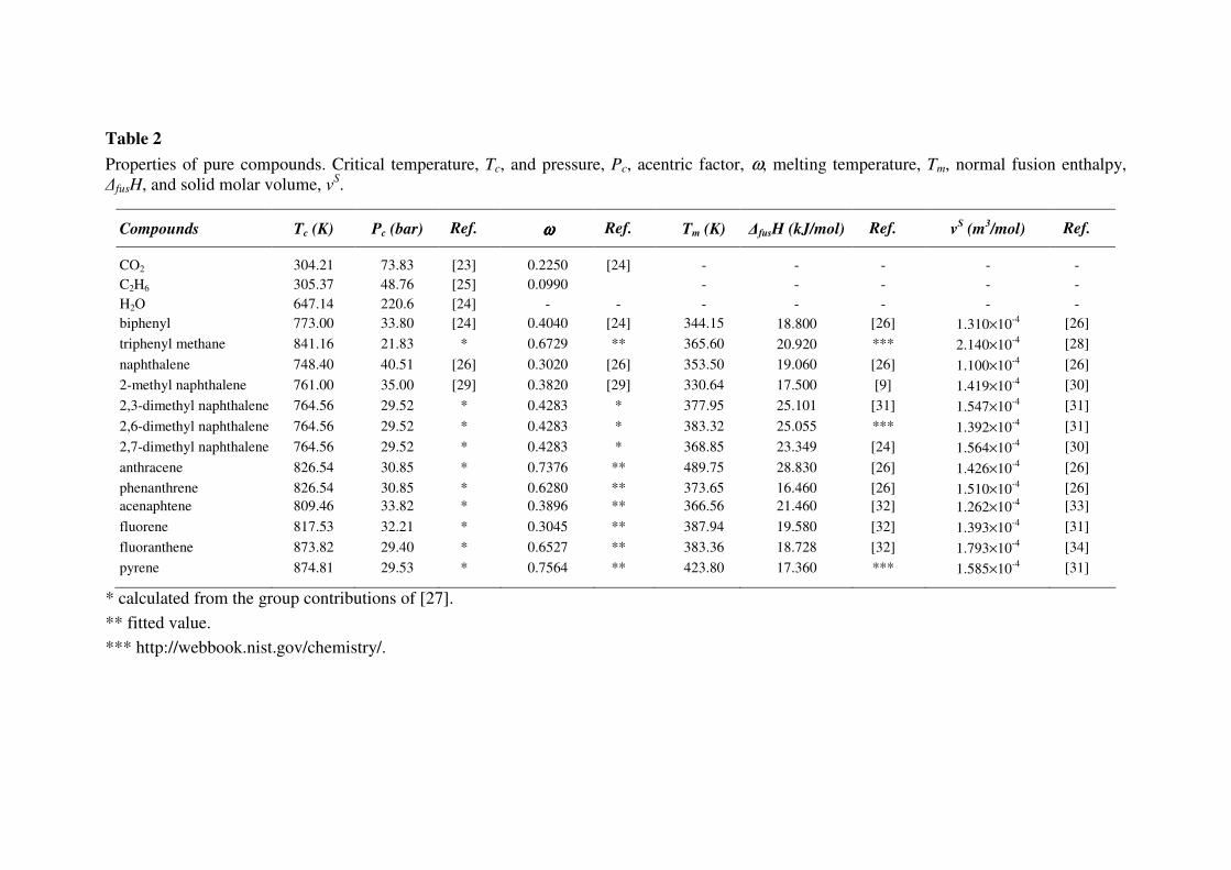
Table 2

Properties of pure compounds. Critical temperature, Tc, and pressure, Pc, acentric factor, ω, melting temperature, Tm, normal fusion enthalpy,

∆fusH, and solid molar volume, vS.

Compounds Tc (K) Pc (bar) Ref. ωωωω Ref. Tm (K) ∆fusH (kJ/mol) Ref. vS (m

3/mol) Ref.

CO2 304.21 73.83 [23] 0.2250 [24] - - - - -

C2H6 305.37 48.76 [25] 0.0990 - - - - -

H2O 647.14 220.6 [24] - - - - - - -

biphenyl 773.00 33.80 [24] 0.4040 [24] 344.15 18.800 [26] 1.310×10-4

[26]

triphenyl methane 841.16 21.83 * 0.6729 ** 365.60 20.920 *** 2.140×10-4

[28]

naphthalene 748.40 40.51 [26] 0.3020 [26] 353.50 19.060 [26] 1.100×10-4

[26]

2-methyl naphthalene 761.00 35.00 [29] 0.3820 [29] 330.64 17.500 [9] 1.419×10-4

[30]

2,3-dimethyl naphthalene 764.56 29.52 * 0.4283 * 377.95 25.101 [31] 1.547×10-4

[31]

2,6-dimethyl naphthalene 764.56 29.52 * 0.4283 * 383.32 25.055 *** 1.392×10-4

[31]

2,7-dimethyl naphthalene 764.56 29.52 * 0.4283 * 368.85 23.349 [24] 1.564×10-4

[30]

anthracene 826.54 30.85 * 0.7376 ** 489.75 28.830 [26] 1.426×10-4

[26]

phenanthrene 826.54 30.85 * 0.6280 ** 373.65 16.460 [26] 1.510×10-4

[26]

acenaphtene 809.46 33.82 * 0.3896 ** 366.56 21.460 [32] 1.262×10-4

[33]

fluorene 817.53 32.21 * 0.3045 ** 387.94 19.580 [32] 1.393×10-4

[31]

fluoranthene 873.82 29.40 * 0.6527 ** 383.36 18.728 [32] 1.793×10-4

[34]

pyrene 874.81 29.53 * 0.7564 ** 423.80 17.360 *** 1.585×10-4

[31]

* calculated from the group contributions of [27].

** fitted value.

*** http://webbook.nist.gov/chemistry/.

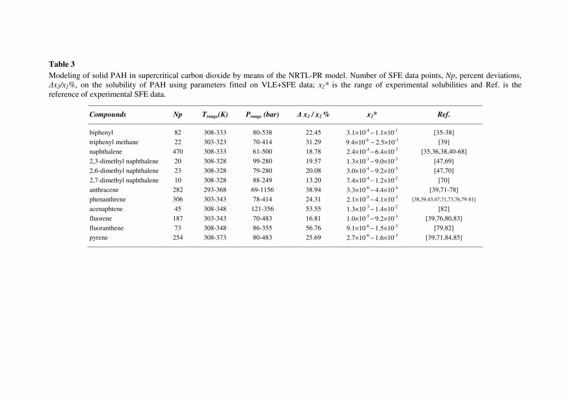
Table 3

Modeling of solid PAH in supercritical carbon dioxide by means of the NRTL-PR model. Number of SFE data points, Np, percent deviations,

∆x2/x2%, on the solubility of PAH using parameters fitted on VLE+SFE data; x2* is the range of experimental solubilities and Ref. is the

reference of experimental SFE data.

Compounds Np Trange(K) Prange (bar) ∆ x2 / x2 % x2* Ref.

biphenyl 82 308-333 80-538 22.45 3.1×10-4

− 1.1×10

-1 [35-38]

triphenyl methane 22 303-323 70-414 31.29 9.4×10-6

− 2.5×10

-3 [39]

naphthalene 470 308-333 61-500 18.78 2.4×10-4

− 6.4×10

-2 [35,36,38,40-68]

2,3-dimethyl naphthalene 20 308-328 99-280 19.57 1.3×10-3

− 9.0×10

-3 [47,69]

2,6-dimethyl naphthalene 23 308-328 79-280 20.08 3.0×10-4

− 9.2×10

-3 [47,70]

2,7-dimethyl naphthalene 10 308-328 88-249 13.20 7.4×10-4

− 1.2×10

-2 [70]

anthracene 282 293-368 69-1156 38.94 3.3×10-6

− 4.4×10

-4 [39,71-78]

phenanthrene 306 303-343 78-414 24.31 2.1×10-5

− 4.1×10

-3 [38,39,43,47,71,73,76,79-81]

acenaphtene 45 308-348 121-356 53.55 1.3×10-3

− 1.4×10

-2 [82]

fluorene 187 303-343 70-483 16.81 1.0×10-5

− 9.2×10

-3 [39,76,80,83]

fluoranthene 73 308-348 86-355 56.76 9.1×10-6

− 1.5×10

-3 [79,82]

pyrene 254 308-373 80-483 25.69 2.7×10-6

− 1.6×10

-3 [39,71,84,85]

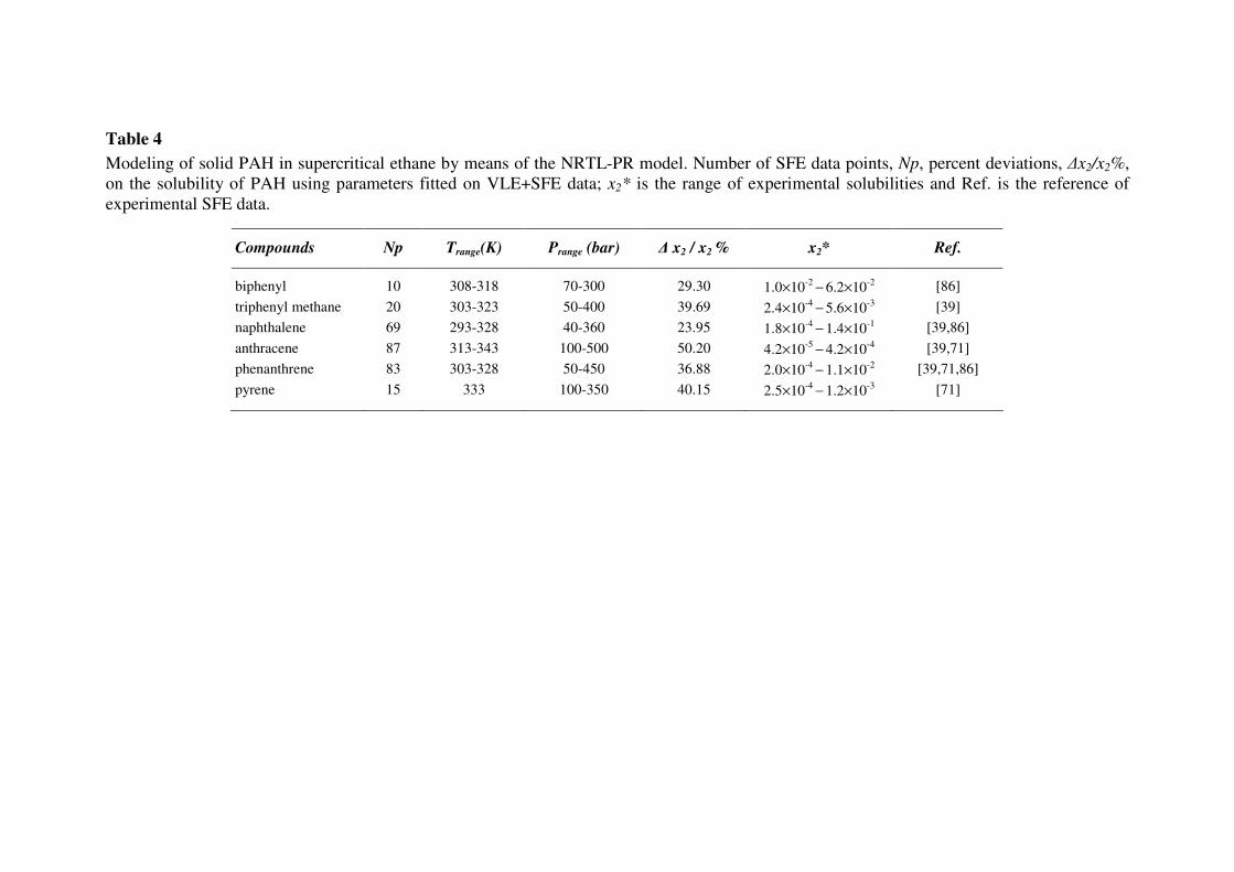
Table 4

Modeling of solid PAH in supercritical ethane by means of the NRTL-PR model. Number of SFE data points, Np, percent deviations, ∆x2/x2%,

on the solubility of PAH using parameters fitted on VLE+SFE data; x2* is the range of experimental solubilities and Ref. is the reference of

experimental SFE data.

Compounds Np Trange(K) Prange (bar) ∆ x2 / x2 % x2* Ref.

biphenyl 10 308-318 70-300 29.30 1.0×10-2

− 6.2×10

-2 [86]

triphenyl methane 20 303-323 50-400 39.69 2.4×10-4

− 5.6×10

-3 [39]

naphthalene 69 293-328 40-360 23.95 1.8×10-4

− 1.4×10

-1 [39,86]

anthracene 87 313-343 100-500 50.20 4.2×10-5

− 4.2×10

-4 [39,71]

phenanthrene 83 303-328 50-450 36.88 2.0×10-4

− 1.1×10

-2 [39,71,86]

pyrene 15 333 100-350 40.15 2.5×10-4

− 1.2×10

-3 [71]

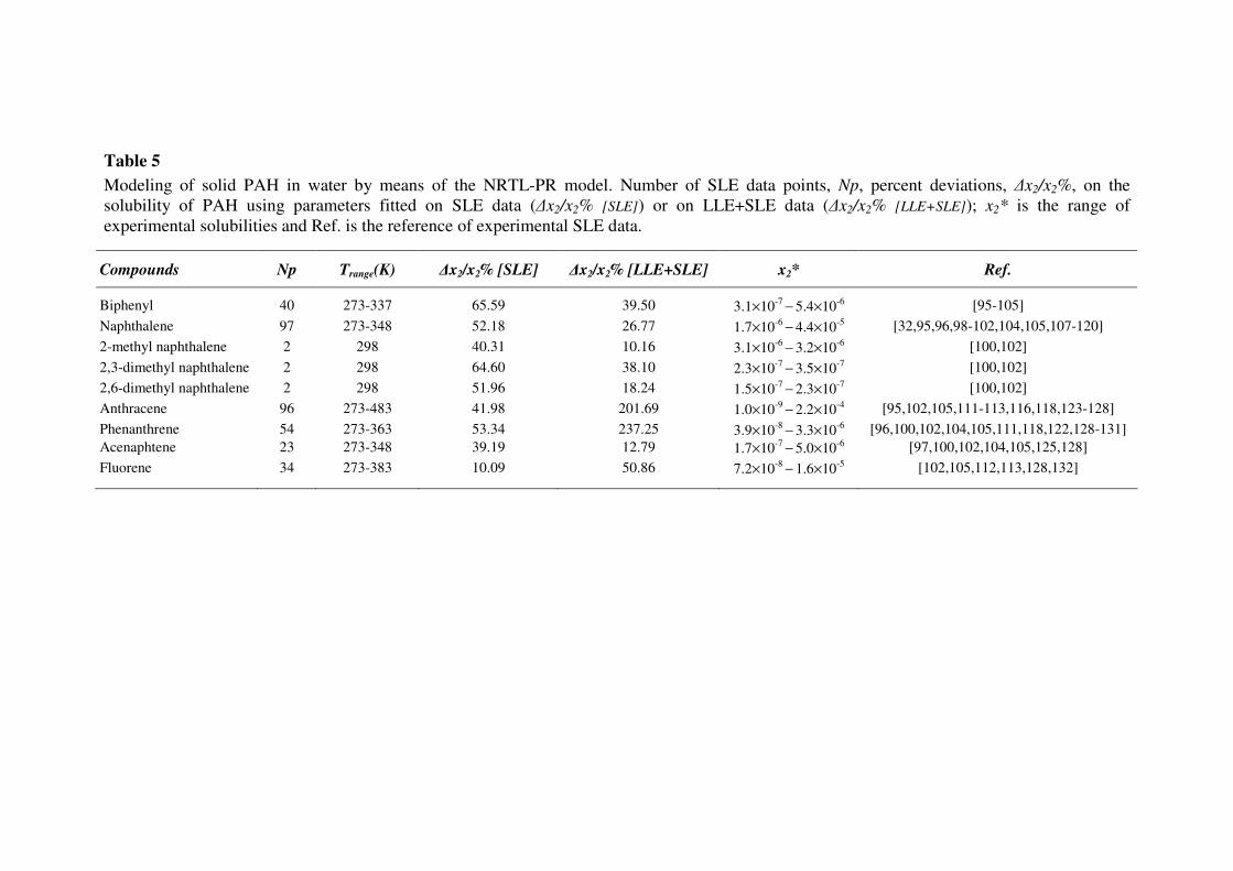
Table 5

Modeling of solid PAH in water by means of the NRTL-PR model. Number of SLE data points, Np, percent deviations, ∆x2/x2%, on the

solubility of PAH using parameters fitted on SLE data (∆x2/x2% [SLE]) or on LLE+SLE data (∆x2/x2% [LLE+SLE]); x2* is the range of

experimental solubilities and Ref. is the reference of experimental SLE data.

Compounds Np Trange(K) ∆x2/x2% [SLE] ∆x2/x2% [LLE+SLE] x2* Ref.

Biphenyl 40 273-337 65.59 39.50 3.1×10-7

− 5.4×10

-6 [95-105]

Naphthalene 97 273-348 52.18 26.77 1.7×10-6

− 4.4×10

-5 [32,95,96,98-102,104,105,107-120]

2-methyl naphthalene 2 298 40.31 10.16 3.1×10-6

− 3.2×10

-6 [100,102]

2,3-dimethyl naphthalene 2 298 64.60 38.10 2.3×10-7

− 3.5×10

-7 [100,102]

2,6-dimethyl naphthalene 2 298 51.96 18.24 1.5×10-7

− 2.3×10

-7 [100,102]

Anthracene 96 273-483 41.98 201.69 1.0×10-9

− 2.2×10

-4 [95,102,105,111-113,116,118,123-128]

Phenanthrene 54 273-363 53.34 237.25 3.9×10-8

− 3.3×10

-6 [96,100,102,104,105,111,118,122,128-131]

Acenaphtene 23 273-348 39.19 12.79 1.7×10-7

− 5.0×10

-6 [97,100,102,104,105,125,128]

Fluorene 34 273-383 10.09 50.86 7.2×10-8

− 1.6×10

-5 [102,105,112,113,128,132]

List of figures

Figure 1. SFE of gas–PAH systems using the NRTL-PR model.

(a) CO2(1) – naphthalene(2) at (□,──) 308K, (◊,─ ─) 318K and (∆,----) 328K. (b) (□,──) CO2(1) – pyrene(2),

(◊,─ ─) CO2(1) – phenanthrene(2), (∆,----) CO2(1) – fluorene(2) and (○, ) CO2(1) – biphenyl(2) at 308K.

(c) C2H6(1) – naphthalene(2) at (□,──) 298K and (◊,─ ─) 308K. (d) (□,──) C2H6 (1) – anthracene(2), (◊,─ ─)

C2H6 (1) – pyrene(2) and (∆,----) C2H6 (1) – phenanthrene (2) at 333K. [Experimental data references given in

Tables 3 and 4]

Figure 2. VLE of gas–aromatic hydrocarbon systems using the NRTL-PR model.

(a) CO2(1) – benzene(2) at (□,──) 273K [87], (◊,─ ─) 313K [88], (∆,----) 347K [89] and (○, ) 414K [90].

(b) C2H6(1) – toluene(2) [91] at (□,──) 313K, (◊,─ ─) 393K and (∆,----) 473K. (c) CO2(1) – naphthalene(2) at

(□,──) 373K [92-94], (◊,─ ─) 403K [94] and (∆,----) 430K [94]. (d) (□,──) CO2(1) – biphenyl(2) [92] and

(◊,─ ─) CO2(1) – phenanthrene(2) [93] at 423K.

Figure 3. LLE of water–aromatic hydrocarbon systems using NRTL-PR [LLE] (──) parameters:

mole fraction of aromatic hydrocarbon in the aqueous phase x2Aq

(◊) and of water in the hydrocarbon

phase x1Org

(□).

(a) Water(1) – benzene(2) [133]: calculations performed under atmospheric pressure. (b) Water(1) – m-

xylene(2) [134]: calculations performed under P = 10 MPa.

Figure 4. SLE of water–aromatic hydrocarbon systems using NRTL-PR [SLE] (──) parameters:

solubility of PAH in water x2 (◊) under atmospheric pressure.

(a) Water(1) – acenaphtene(2). (b) Water(1) – phenanthrene(2). [Experimental data references given in Table

5]

Figure 5. LLE of water–aromatic hydrocarbon systems using NRTL-PR [LLE] (──) or [LLE+SLE]

(─ ─) parameters: mole fraction of aromatic hydrocarbon in the aqueous phase x2Aq

(◊) and of water

in the hydrocarbon phase x1Org

(□) under atmospheric pressure.

(a) Water(1) – toluene(2) [135]. (b) Water(1) – p-xylene(2) [134].

Figure 6. SLE of water–aromatic hydrocarbon systems using NRTL-PR [SLE] (──) or [LLE+SLE]

(─ ─) parameters: solubility of PAH in water x2 (◊).

(a) Water(1) – naphthalene(2): calculations performed under atmospheric pressure. (b) Water(1) – fluorene(2):

calculations performed under P = 5 MPa. [Experimental data references given in Table 5]

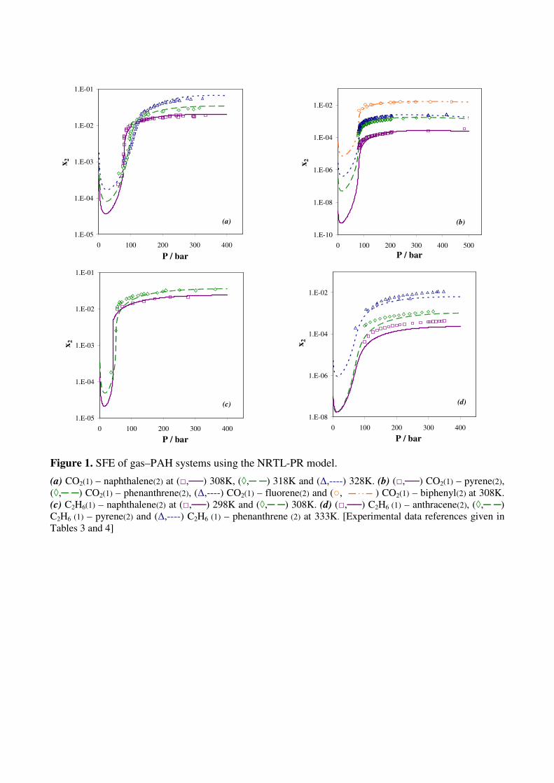
Figure 1. SFE of gas–PAH systems using the NRTL-PR model.

(a) CO2(1) – naphthalene(2) at (□,──) 308K, (◊,─ ─) 318K and (∆,----) 328K. (b) (□,──) CO2(1) – pyrene(2),

(◊,─ ─) CO2(1) – phenanthrene(2), (∆,----) CO2(1) – fluorene(2) and (○, ) CO2(1) – biphenyl(2) at 308K.

(c) C2H6(1) – naphthalene(2) at (□,──) 298K and (◊,─ ─) 308K. (d) (□,──) C2H6 (1) – anthracene(2), (◊,─ ─)

C2H6 (1) – pyrene(2) and (∆,----) C2H6 (1) – phenanthrene (2) at 333K. [Experimental data references given in

Tables 3 and 4]

1.E-05

1.E-04

1.E-03

1.E-02

1.E-01

0 100 200 300 400

P / bar

x2

1.E-10

1.E-08

1.E-06

1.E-04

1.E-02

0 100 200 300 400 500

P / bar

x2

1.E-05

1.E-04

1.E-03

1.E-02

1.E-01

0 100 200 300 400

P / bar

x2

1.E-08

1.E-06

1.E-04

1.E-02

0 100 200 300 400

P / bar

x2

(a) (b)

(c) (d)

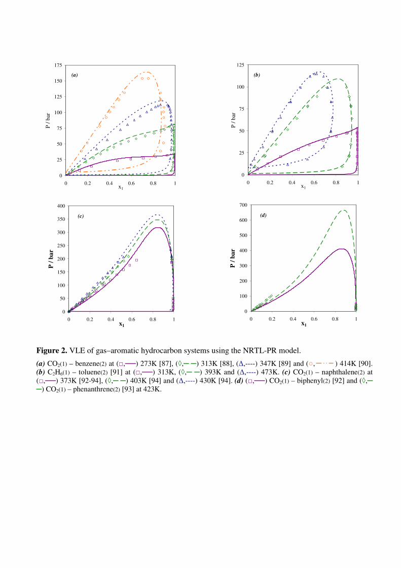
Figure 2. VLE of gas–aromatic hydrocarbon systems using the NRTL-PR model.

(a) CO2(1) – benzene(2) at (□,──) 273K [87], (◊,─ ─) 313K [88], (∆,----) 347K [89] and (○, ) 414K [90].

(b) C2H6(1) – toluene(2) [91] at (□,──) 313K, (◊,─ ─) 393K and (∆,----) 473K. (c) CO2(1) – naphthalene(2) at

(□,──) 373K [92-94], (◊,─ ─) 403K [94] and (∆,----) 430K [94]. (d) (□,──) CO2(1) – biphenyl(2) [92] and (◊,─

─) CO2(1) – phenanthrene(2) [93] at 423K.

0

25

50

75

100

125

0 0.2 0.4 0.6 0.8 1x1

P /

bar

0

25

50

75

100

125

150

175

0 0.2 0.4 0.6 0.8 1x1

P /

bar

(a) (b)

0

50

100

150

200

250

300

350

400

0 0.2 0.4 0.6 0.8 1x1

P /

ba

r

0

100

200

300

400

500

600

700

0 0.2 0.4 0.6 0.8 1x1

P /

ba

r

(d) (c)

Figure 3. LLE of water–aromatic hydrocarbon systems using NRTL-PR [LLE] (──) parameters: mole

fraction of aromatic hydrocarbon in the aqueous phase x2Aq

(◊) and of water in the hydrocarbon phase

x1Org

(□).

(a) Water(1) – benzene(2) [133]: calculations performed under atmospheric pressure. (b) Water(1) – m-xylene(2)

[134]: calculations performed under P = 10 MPa.

1.E-04

1.E-03

1.E-02

1.E-01

250 275 300 325 350 375 400

T / K

log x

2A

q, x

1O

rg

1.E-05

1.E-04

1.E-03

1.E-02

1.E-01

1.E+00

250 300 350 400 450 500

T / Klo

g x

2A

q, x

1O

rg

(a) (b)

Figure 4. SLE of water–aromatic hydrocarbon systems using NRTL-PR [SLE] (──) parameters:

solubility of PAH in water x2 (◊) under atmospheric pressure.

(a) Water(1) – acenaphtene(2). (b) Water(1) – phenanthrene(2). [Experimental data references given in Table 5]

(a) (b)

1.E-07

1.E-06

1.E-05

1.E-04

250 275 300 325 350 375 400

T / K

log x

2

1.E-08

1.E-07

1.E-06

1.E-05

250 275 300 325 350 375 400

T / K

log x

2

Figure 5. LLE of water–aromatic hydrocarbon systems using NRTL-PR [LLE] (──) or [LLE+SLE] (─

─) parameters: mole fraction of aromatic hydrocarbon in the aqueous phase x2Aq

(◊) and of water in the

hydrocarbon phase x1Org

(□) under atmospheric pressure.

(a) Water(1) – toluene(2) [135]. (b) Water(1) – p-xylene(2) [134].

1.E-05

1.E-04

1.E-03

1.E-02

1.E-01

250 275 300 325 350 375 400

T / K

log x

2A

q, x

1O

rg

(a) (b)

1.E-05

1.E-04

1.E-03

1.E-02

1.E-01

250 275 300 325 350 375 400

T / Klo

g x

2A

q, x

1O

rg

Figure 6. SLE of water–aromatic hydrocarbon systems using NRTL-PR [SLE] (──) or [LLE+SLE] (─

─) parameters: solubility of PAH in water x2 (◊).

(a) Water(1) – naphthalene(2): calculations performed under atmospheric pressure. (b) Water(1) – fluorene(2):

calculations performed under P = 5 MPa. [Experimental data references given in Table 5]

(a) (b)

1.E-07

1.E-06

1.E-05

1.E-04

250 275 300 325 350 375 400

T / K

log x

2

1.E-08

1.E-07

1.E-06

1.E-05

1.E-04

250 275 300 325 350 375 400 425

T / K

log x

2