

1 of 16
PROCEEDINGS, Thirty-Eighth Workshop on Geothermal Reservoir Engineering
Stanford University, Stanford, California, February 11-13, 2013
SGP-TR-198
PRELIMINARY INVESTIGATION OF RESERVOIR DYNAMICS MONITORED THROUGH
COMBINED SURFACE DEFORMATION AND MICRO-EARTHQUAKE ACTIVITY:
BRADY’S GEOTHERMAL FIELD, NEVADA
Nicholas C. DAVATZES1, Kurt L. FEIGL
2, Robert J. MELLORS
3, William FOXALL
3,
Herbert F. WANG2, and Peter DRAKOS
4
1Temple University1901 N. 13 Street;
EES, Beury Hall, Rm. 307
Philadelphia, PA 19122
e: [email protected], T: 215-204-2319 2University of Wisconsin Madison,
3Lawrence Livermore National Laboratory,
4ORMAT
ABSTRACT
Fluid pressure change accompanying pumping in
the Bradys Geothermal Field is associated with two
complimentary deformation responses: (1) surface
deformations sensible by InSAR corresponding to
thermo-poroelastic deformations resulting in volume
changes and (2) seismic slip on fractures induced by
either changes in effective normal stress or solid
stress with minimal impact to volume but potential
impact on permeability structure due to dilation or
compaction. We present an integrated data set that
compares the impulse from pumping to the
deformation response in order to investigate the
coupling of these behaviors, and to constrain the
geometry and rheology of the reservoir and
surrounding crust.
We find that surface deformation is strongly
associated with the location of the production wells,
with associated subsidence concentrated within a
bend in the Bradys normal fault. A broader region of
minor subsidence extends several kilometers to the
NNE and SSW along the fault trend. Interestingly,
MEQs are absent within the region of intense
subsidence where effective stress stabilizing fractures
are expected to be high but are broadly distributed in
and around the margins of the region of minor
subsidence below the reservoir depth. MEQs are also
densely distributed along the Bradys fault from
injectors to producers where effective stresses are
expected to be lower. Initial modeling indicates that
the pattern of subsidence is consistent with fluid
extraction along a vertical conduit from shallow
depths to approximately 1 km within the fault bend
and then extraction at ~1 km along the entire length
of the mapped Brady‟s fault indicating a reservoir
much larger than would be expected from the
footprint of the production wells. The planned EGS
stimulation well 15-12ST1 is located SSW of this
permeable volume associated with production along
the direction of SHmax , which is also the anticipated
direction of stimulation growth, and east of the
deeper reservoir volume in a low permeability
volume adjacent to the reservoir. Although the spatial
patterns provide relatively clear insights, we find that
temporal correlations are complex and that both
surface deformation and seismicity rates are highly
variable in time, but that simple correlations to
changes in pumping rate, which varies by ~15-20%,
are not yet obvious. This complexity, and resulting
limitations on predicting responses, is expected given
the long history of stressing by production and
geologic complexity and will be addressed in a future
study modeling the pressure diffusion due to
pumping and related deformation response.
INTRODUCTION
Management or stimulation of a geothermal
reservoir involves manipulating the fluid pressure at
depth to exploit, maintain, or create permeability.
Because relatively few tools are available to map the
permeability distribution, most of the reservoir
volume is poorly characterized with respect to fluid
flow. Stimulation via fluid injection at wells causes
two distinct effects throughout the reservoir and
beyond: (1) slip on fractures that can often be
detected as seismic events using seismology and (2)
expansion or contraction that can be detected as
deformation of the ground surface using geodesy.
The use of seismicity to map an evolving permeable
network presumes that the percolation of fluid
pressure initiates shear failure of fractures due to the
reduction of normal stress resulting in slip and/or
creates new opening-mode fractures, and that these

failure events are sensible through microseismic
monitoring thus revealing the extent of the volume
sustaining large fluid pressure changes. However, the
displacement of fracture walls may be either aseismic
or below the detection threshold of the local seismic
network, thus limiting the completeness of MEQ
mapping of fluid pressure variation. In addition,
pumping induces volume changes in the rock add an
additional source of stressing that further
complications the relationship between MEQs and
the transport of fluids and pressure within the
reservoir.
These same volume changes resulting from fluid
injection and extraction are manifested as surface
deformation that can be measured by Interferometric
Synthetic Aperture Radar (InSAR). The resulting
geodetic measurements provide an independent
constraint on models for the deforming reservoir.
By comparing these two responses to pressure
variation due to pumping in the reservoir, we
investigate three key issues:
1. Does the seismicity coincides with volume
changes at depth due to fluid pressure
fluctuations inferred from surface
deformations?
2. What proportion of the deformation observed
at the surface can be correlated to sensible
seismic processes?
3. How do pressure change, seismicity, and
permeability structure correlate in time?
At the Brady‟s geothermal field, we have begun
testing these relationships using the time series of
injection and extraction forcing the reservoir with
time series of micro-seismic events recorded by a
local seismic network and corresponding
measurements of surface deformation from InSAR.
In this paper, we investigate the first two issues
during a time interval of normal reservoir activity
from October 2010 through January 2013, and
preceding the planned EGS stimulation of well 15-
12ST1.
GEOLOGIC SETTING
The Brady‟s Geothermal Field is located in
western Nevada within a region of distributed
extension associated with the NE terminus of the
Walker Lane (Faulds et al., 2011; see summary in
Blake and Davatzes, 2012). The reservoir is located
along a complex series of normal faults (Faulds and
Garside, 2003; Faulds, 2010) at a prominent bend,
which is also associated with surface hydrothermal
activity (Coolbaugh et al., 2004) (Figure 1).
Production wells are generally clustered at this bend,
with injection wells primarily located to the NE along
the fault trace associated with surface hydrothermal
activity.
Standard production and injection of the
reservoir has been carried from 1992 to present. It is
characterized by pressure drawdown with minimal
cooling and subsidence. Six production wells and 2
primary injection wells are distributed over a 1.4 km
region along the fault with an average depth of 930
m; production wells range in depth from 400 m to
1770 m (Figure 1). Vertical displacements associated
with past and current production (Figure 1) center on
production wells and appear to extend over a 7 km
region, extending significantly beyond the surface
expression of the Brady‟s fault system but aligned
with it (Oppliger et al., 2006). Since 2010, seismicity
(Figure 1), albeit at low rates, has been detected by a
local seismometer array managed by Lawrence
Berkeley National Laboratory as part of the EGS
preparation (Nathwani et al., 2011) and deployed to
maximize sensitivity around the planned 15-12ST1
EGS well.
Early in 2013, a hydraulic stimulation is planned
in well 15-12ST1 to extend the reservoir, which will
be characterized by long-duration, variable pressure
injection, and once on-line, long-term low pressure
cold-water injection. This might be accompanied by
microseismicity indicating pore pressure invasion of
natural fractures and limited pore pressure rise in the
matrix porosity. Following stimulation, any newly
stimulated permeable network will experience pore
pressure perturbations from both injection and
production as it is incorporated into the reservoir.
DEFORMATION
The surface deformation measurements in this
study use an imaging geodetic technique called
InSAR (Interferometric Synthetic Aperture Radar).
This technique uses pairs of satellite radar images
taken at different times to infer the relative change in
surface position during the intervening period. The
change is calculated from the interference pattern
caused by the difference in phase between the two
images acquired by the space-borne radar sensor at
two distinct times. As the InSAR measurements are
made with respect to the line-of sight to the satellite,
the measurement includes both vertical and
horizontal components of surface motion.
Unfortunately, although the sensitivity to both
components can be calculated for a specific sensor, it
is not possible to uniquely distinguish vertical and
horizontal components with only a single
measurement. These results provide a high spatial
sampling density (~100 pixels/km2). Errors are
typically due to poorly imaged (decorrelated) areas,
atmospheric artifacts caused by variations in water
vapor, satellite orbit errors, or inaccuracies in the
digital elevation model used to make corrections.
3 of 16
Fig
ure
1:
Bra
dys
Fa
ult
, S
eism
icit
y, a
nd
Su
bsi
den
ce M
ap
s:
(a)
Geo
log
ic i
nd
ex m
ap
an
d s
tres
s m
od
el.
Th
e fa
ult
ma
p i
s fr
om
Fa
uld
s (2
01
0)
and
su
rfa
ce
hyd
roth
erm
al
act
ivit
y is
fro
m C
oo
lba
ugh
et
al.
(2
00
4).
Als
o i
nd
ica
ted
are
th
e lo
cati
on
s o
f in
ject
ion
and
pro
du
ctio
n w
ells
, a
nd
EG
S w
ell
15
-
12
ST
1.
Th
e st
ress
mo
del
is
fro
m M
oo
s (u
np
ub
lish
ed r
epo
rt,
20
11
) a
nd
ref
lect
s th
e a
na
lysi
s o
f in
sit
u r
ock
str
eng
th,
a d
ensi
ty l
og
, a
n
equ
ilib
rate
d P
TS
lo
g,
dri
llin
g-i
nd
uce
d b
ore
ho
le d
efo
rma
tio
n r
evea
led
in
im
ag
e lo
gs
of
15
-12
and
15
-12S
T1
, an
d a
min
i-h
ydra
uli
c fr
act
uri
ng
test
. T
he
stre
ss m
od
el i
s su
mm
ari
zed
as
an
ou
ter
red
rin
g c
ente
red
on
15
-12
ST
1 c
orr
esp
on
din
g t
o t
he
vert
ica
l st
ress
, a
n i
nn
er b
lue
rin
g
corr
esp
on
din
g t
o t
he
sta
tic
flu
id p
ress
ure
as
a f
ract
ion
of
the
vert
ica
l st
ress
, a
nd
th
e m
ean
ho
rizo
nta
l p
rin
cip
al
stre
ss d
irec
tio
ns
+/-
1
sta
nd
ard
dev
iati
on
are
in
dic
ate
d b
y th
e th
ick
bla
ck l
ine
an
d y
ello
w w
edg
es.
Th
e le
ng
ths
of
thes
e b
lack
lin
es
sum
ma
rize
th
e sc
ali
ng
bet
wee
n
the
ho
rizo
nta
l p
rin
cip
al
stre
ss m
ag
nit
ud
es a
nd t
he
vert
ical
stre
ss.
(b)
Sei
smic
ity
det
ecte
d b
y th
e lo
cal
seis
mo
met
er n
etw
ork
. T
he
ma
p o
f
seis
mic
ity
is c
olo
r-co
ded
by
da
te a
nd
is
con
sist
ent
wit
h a
ll s
ub
seq
uen
t fi
gu
res.
(c)
Su
rfa
ce d
efo
rma
tio
ns
ma
pp
ed b
y In
SA
R.
Th
e o
utl
ine
of
the
reg
ion
su
sta
inin
g s
ub
sid
ence
(g
reen
) a
nd
in
ten
se s
ub
sid
ence
(o
ran
ge-y
ello
w)
inte
rpre
ted
fro
m t
he
inte
rfer
og
ram
in
th
e ri
gh
t-h
an
d p
an
el a
re
als
o i
nd
ica
ted
. T
he
mo
del
of
def
orm
ati
on
so
urc
es u
sed
to
in
terp
ret
the
surf
ace
def
orm
ati
on
s in
clu
des
tw
o h
ori
zon
tal
Oka
da
rec
tang
ula
r a
nd
two
Mo
gi
po
int
sou
rces
are
plo
tted
in
(b).
Ma
ps
are
in
Un
iver
sal
Tra
nsv
erse
Mer
cato
r (z
on
e 1
1)
pro
ject
ion
.

4 of 16
Measurement precision depends on the sensor
wavelength, which varies among satellites, but 10
mm is a reasonable estimate. This remote-sensing
tool has been demonstrated and validated for many
actively deforming areas, including natural
earthquakes and anthropogenic activity (e.g.,
Massonnet and Feigl, 1998). InSAR data products are
typically registered to a digital elevation model
(DEM) in geographic or cartographic coordinates to
within ~10 m. The Brady‟s area, which is relatively
arid and lacks extreme topographic variations, is well
suited for InSAR.
InSAR observations
Previous studies using 5 cm wavelength (C-
band) data (e.g. Oppliger et al., 2006) demonstrated
the usefulness of InSAR for the Brady‟s area and
suggested 10 mm per year of line-of-sight motion.
We have analyzed synthetic aperture radar (SAR)
data acquired by four previous satellite missions and
from two ongoing missions. The archival missions
include data from 1992 to 2010 and includes 61
scenes from the C-band ERS-1, ERS-2, Envisat (e.g.
McLeod et al., 1998) as well as 36 images from the
21 cm (L-band) ALOS (Rosenqvist et al., 2007).
These data sets were acquired from the WINSAR
(http://winsar.unavco.org/) and Alaska SAR facility
data centers (http://www.asf.alaska.edu/). This
represents a much larger data set than previous
studies. In general, this dataset shows a consistent
pattern of deformation over time dating back to 1992.
The current study concentrates on SAR images
covering the study area from 2011 to 2012, which
overlaps with the available seismic data. Current data
collection (3.1 cm; X-band) is from the ongoing
TanDEM and TerraSAR-X satellites (Kieger et al.,
2007; Pitz and Miller, 2010). Thirty-six scenes have
been collected in 2011 and 2012. This new data is
processed using the Diapason InSAR processing
software (CNES, 2006) developed by the French
Space Agency, CNES, as described previously
(Massonnet and Rabaute, 1993, Massonnet et al.,
1993, Massonnet and Feigl, 1998). The wrapped
phase values are filtered and resampled using a quad-
tree algorithm called PHA2QLS (Ali and Feigl, 2012,
Feigl and Sobol, 2013).
The rate of deformation is not constant. After a
preliminary analysis of the deformation, we find
especially rapid deformation during a three-month
time interval in autumn 2011, using data from the
TanDEM-X satellite mission (Krieger et al., 2007)
(Figure 2). However, during other epochs,
preliminary analysis has revealed that this
deformation rate is highly variable (not presented
here). The principal signal in the interferogram is an
elongated pattern of range change centered on
Brady‟s Hot Springs consistent with subsidence. The
total line-of-sight deformation in this interferogram is
approximately 3 cm which corresponds to 2.1 cm of
subsidence (incidence angle of 44 from vertical) and
assuming pure vertical motion occurring within the
88 day period (Figure 3).
Figure 2. Interferograms for Brady’s Hot Springs, spanning the 88-day time interval from 2011 SEP 24 to 2011 DEC
21. The panels include (a) observed phase values; (b) modeled phase values calculated from the final
estimate of the parameters in the elastic model; (b) cartoon of modeled deformation sources; (d) final
residual phase values formed by subtracting final modeled values from observed phase values; and (e)
angular deviations for final estimate. Asterisk indicates the location of centroid of the modeled sill. One
cycle of phase denotes 15.5 mm of range change. The Tandem-X orbit numbers are 6984 and 8320 in
Strip 14 of Track 167.

5 of 16
InSAR signal is not an artifact
Before interpreting the InSAR observations in
terms of deformation on the ground, we consider, and
then reject, three other possibilities.
The first possibility is that uncertainties in the
orbital trajectories for the TANDEM-X spacecraft are
responsible for the observed fringe pattern. To test
this hypothesis, we estimate the orbital parameters
from the interferometric fringe pattern using the
approach proposed by Kohlhase et al. (2003),
implemented as the General Inversion of Phase
Technique (GIPhT) by Feigl and Thurber (2009), and
extended to the gradient of wrapped phase by Ali and
Feigl (2012). The estimated values do not differ
significantly from zero with 95% confidence for the
radial and along-track components of the spacecraft‟s
position and velocity vectors. Each of these four
parameters is estimated at each of the acquisition
epochs, except the first one in a tree, when the
adjustment is arbitrarily set to zero to regularize the
solution (Feigl and Thurber, 2009). This conclusion
is consistent with our intuitive expectation that orbital
errors do not generate closed fringes.
The second possibility is that atmospheric
perturbations contribute to the observed fringe
pattern. To evaluate this possibility, we estimate the
vertical component of the range change gradient
to be 10 ± 3 parts per million of
topographic relief using GIPhT. Although this value
indicates a relatively large tropospheric perturbation
(Hanssen, 2001), it would contribute less than ~1.5
mm in range or less than ~0.1 fringe to the C-band
interferograms considered here because the
(differential) topographic relief is less than ~150 m
across the study area.
The third possibility, that an error in the digital
elevation model (DEM) creates an artifact in the
InSAR results, can be excluded by two arguments:
one qualitative and one quantitative. First, the shape
of the observed fringe pattern does not resemble that
of the topographic relief or that produced by
interpolation of incorrect elevations (e.g., Massonnet
and Feigl, 1995). Second, the signal observed in the
fringe patterns is much too large to be explained by
an error in the DEM. Derived from the U.S. National
Elevation Dataset (Falorni et al., 2005, Gesch et al.,
2002), the DEM used to account for the topographic
contribution to the interferograms has an absolute,
vertical uncertainty of no worse than σh ~ 20 m in
elevation (Kellndorfer et al., 2004). For example, the
interferometric pair shown in has an orbital
configuration such that the altitude of ambiguity ha is
~400 m. The definition of ha (Massonnet and Feigl,
1998) implies that a hypothetical artifact in the DEM
would have to be 2ha ~ 800 m in elevation to create
the 2-cycle signature in the observed fringe pattern
(Figure a). Such an artifact is extremely unlikely
because it exceeds the DEM uncertainty by a factor
of 2ha/σh ~ (800 m)/(20 m) ~ 40. Furthermore, in the
case of a hypothetical artifact in the DEM, the
number of fringes would be inversely proportional to
the altitude of ambiguity ha in each pair (e.g.,
Massonnet and Feigl, 1995). In fact, however, the
number of fringes is roughly proportional to the time
interval spanned by the interferometric pair.
From the preceding three arguments, we
conclude that the signal observed in the InSAR
results is due to deformation on the ground.
Interpreting the deformation using an elastic
model of production and injection
In this section, we analyze the deformation on
the ground by estimating parameters in a geophysical
model using GIPhT (Feigl and Thurber, 2009, Ali
and Feigl, 2012). The model attributes the
deformation to changes in volume of the reservoir,
describing production wells as sinks and injection
wells as sources. The model assumes an elastic
rheology with uniform material properties
everywhere in a half space. The shear modulus (or
rigidity) G and Poisson‟s ratio ν are also adjustable
parameters. The model includes three sinks and one
source.
The sinks in the model interpret the observed
deformation as the result of extracting fluids from the
crust by geothermal production. The main part of the
producing reservoir is described as a horizontal,
rectangular prism at a depth of 1.1 ± 0.2 km. It
decreases in volume at a rate of dV/dt = –268 × 103
m3/yr (using a dislocation formulation with 9 free
parameters (Okada, 1985). The estimated values of
the model parameters, along with their uncertainties,
are listed in Appendix 1.
The second and third sinks are each modeled as
deflating spheres (Mogi, 1958, Segall, 2010).
Located at a depth of 299 ± 38 m, the first sink is
deflating with rate dV/dt = -10 ± 4 × 10³ m
3/yr (–5 ±
2 gallons/minute). Located at a depth of 298 ± 66 m,
the second sink is deflating with rate dV/dt = -13 ± 5
× 103 m
3/yr (= –6 ± 2 gallons/minute).
The injection into wells 18D-31and 18B-31 is
modeled as a horizontal, rectangular prism at a (very
shallow) depth of 37 ± 38 m. Its volume increases at
a rate of dV/dt = 16 × 103 m
3/yr (= +8
gallons/minute). using a dislocation formulation with
9 free parameters (Okada, 1985).
The total net change in volume between 2011
SEP 24 and 2011 DEC 21 is ΔV = -67 ± 8 × 10³ m
3
(= 18 ± 2 million gallons = 2.4 ± 0.2 million cubic
feet).
6 of 16
The resulting modeled phase values shown in
Figure b reproduce the elongated pattern of the
observed phase values shown in a. Their difference,
the wrapped residual phase values shown in Figure c,
exhibit less than one fringe of unexplained signal.
This model fits the resampled InSAR observations to
within 0.0494 cycles (0.7 mm), as measured by the
circular mean deviation of the phase residuals, the
objective function minimized by GIPhT. Considering
the angular deviations of all the pixels in the 88-day
interferogram (Figure d), we find their circular mean
deviation to be 0.0801 cycles (1.2 mm).
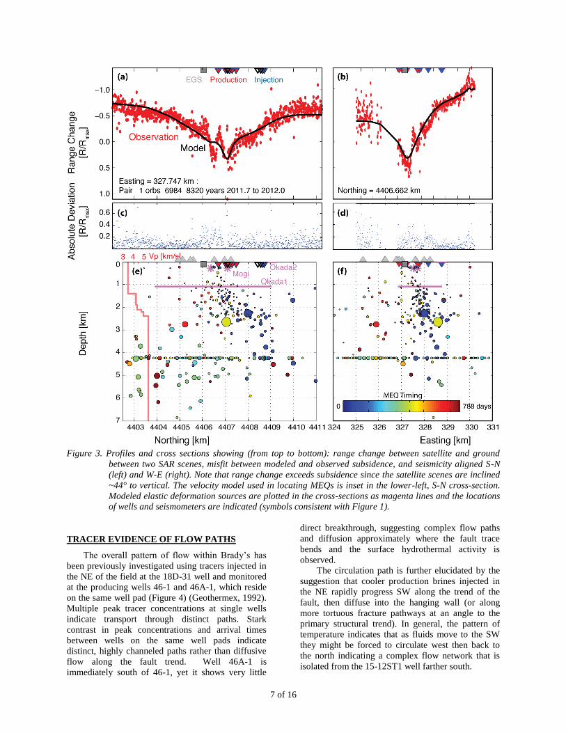
These models are most easily evaluated along
profiles of range change that reveal the agreement
between model and data for the interferogram. Two
profiles are shown, one trending south-to-north
profile along Easting 327.747 km capturing the
overall separation of production and injection wells,
and a second west-to-east along Northing 4406.662
km that is at a high angle to the trend of the fault
systems. Both transects pass through the region of
maximum subsidence (Figures 1 and 2). The solid
black curve shows the modeled value of range
change calculated from the final deformation model
that minimizes the misfit. The circles show the
observed range change calculated by multiplying the
unwrapped observed phase value by 15.5 mm/cycle.
The phase values have been unwrapped by adding the
final modeled values to the final residual values. By
construction, the filled circles must fall within ± ½
cycle of the model curve.
SEISMICITY
Microearthquake Locations, Magnitudes and
Seismic Moments
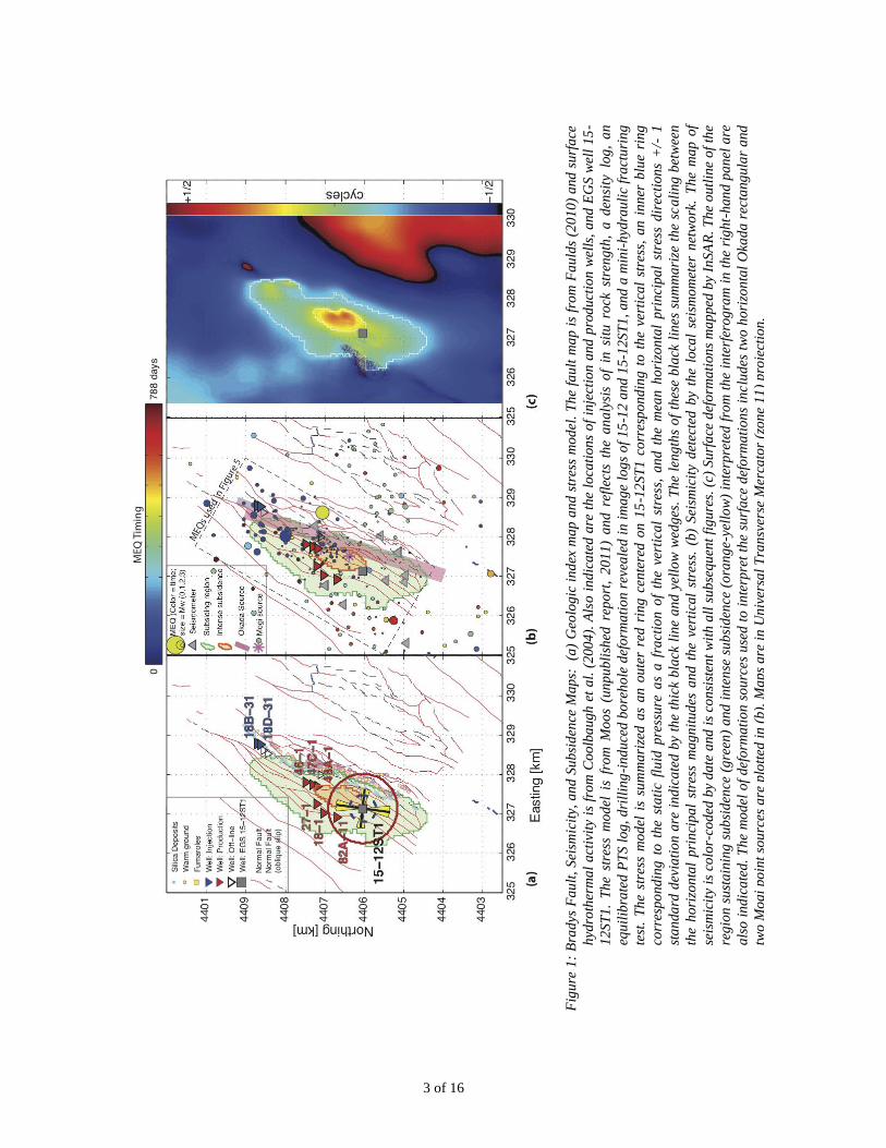
The microearthquake locations plotted on
Figures 1 and 3 are from the Lawrence Berkeley
National Laboratory (LBNL) Brady‟s seismicity
catalog for the period November, 2010 to January,
2013. The locations are routinely calculated from
data recorded by the Brady‟s local seismic network
and displayed in near-real time on the LBNL web site
(http://esd.lbl.gov/research/projects/induced_seismici
ty/egs/desert_peak_brady.html). The Brady‟s
network was installed around well 15-12ST1
specifically to monitor seismicity induced by the
upcoming stimulation in the well. In its current
configuration the network comprises five borehole
(depths 15 m to 90 m) and four surface three-
component sensors. All of the routine processing of
the Brady‟s data stream is carried out automatically.
Locations are calculated from automatic P- and S-
wave arrival time picks using the preliminary
velocity model shown on Figure 3. The shallow
velocities in the model are based on a vertical seismic
profile from the Desert Peak geothermal field located
approximately 6 km southeast of Brady‟s. Moment
magnitudes (Mw) are calculated from static seismic
moments estimated from the long-period levels of
automatically determined microearthquake (MEQ)
source displacement amplitude spectra. Cumulative
seismic moment release is shown on Figure 5. The
calculated magnitudes of events recorded during this
period range from -1 to 2.4.
The accuracy of the MEQ locations and size
estimates is limited by three factors. The first is the
precision of the automatic arrival time picks and
spectral fits, which would undoubtedly be improved
by manual checks. The second factor is that most of
the microearthquakes located to date fall outside of
the network coverage, and are therefore relatively
poorly constrained by the recorded data. This limits
in particular the depth resolution of events located at
distances greater than about one network aperture
from the nearest station. The apparent lineation at
4.3 km depth on Figure 3c corresponds to poorly
constrained locations for which the depth was held
fixed at an assumed 3 km below sea level in order to
obtain an epicentral solution. Finally, it is not known
at present how well the preliminary velocity model
represents the actual shallow velocity structure at
Brady‟s (S. Jarpe, LBNL, personal communication),
which also contributes to the uncertainty in the
locations.
Microearthquake activity and locations
The largest concentration of MEQs is located to
the north of the network between the injection and
production wells (Figure 1). The majority of the
events within this concentration occurred in two
bursts of activity, the first on February 3 and 4, 2011,
and a second smaller cluster of events on April 2,
2012 (Figure 5). More recently, in January 2013,
there as been increased earthquake activity, but these
events are more widely distributed, with the largest
events to the SW of the geothermal field.
7 of 16
Figure 3. Profiles and cross sections showing (from top to bottom): range change between satellite and ground
between two SAR scenes, misfit between modeled and observed subsidence, and seismicity aligned S-N
(left) and W-E (right). Note that range change exceeds subsidence since the satellite scenes are inclined
~44° to vertical. The velocity model used in locating MEQs is inset in the lower-left, S-N cross-section.
Modeled elastic deformation sources are plotted in the cross-sections as magenta lines and the locations
of wells and seismometers are indicated (symbols consistent with Figure 1).
TRACER EVIDENCE OF FLOW PATHS
The overall pattern of flow within Brady‟s has
been previously investigated using tracers injected in
the NE of the field at the 18D-31 well and monitored
at the producing wells 46-1 and 46A-1, which reside
on the same well pad (Figure 4) (Geothermex, 1992).
Multiple peak tracer concentrations at single wells
indicate transport through distinct paths. Stark
contrast in peak concentrations and arrival times
between wells on the same well pads indicate
distinct, highly channeled paths rather than diffusive
flow along the fault trend. Well 46A-1 is
immediately south of 46-1, yet it shows very little
direct breakthrough, suggesting complex flow paths
and diffusion approximately where the fault trace
bends and the surface hydrothermal activity is
observed.
The circulation path is further elucidated by the
suggestion that cooler production brines injected in
the NE rapidly progress SW along the trend of the
fault, then diffuse into the hanging wall (or along
more tortuous fracture pathways at an angle to the
primary structural trend). In general, the pattern of
temperature indicates that as fluids move to the SW
they might be forced to circulate west then back to
the north indicating a complex flow network that is
isolated from the 15-12ST1 well farther south.

8 of 16
Figure 4: (a) Results of pre-production tracer test
conducted April-May 1992 in which 200 lb
of fluoroscein tracer was injected into well
18D-31 and monitored in wells 46-1 and
46A-1 (GeothermEx, 1992). (b) Interpreted
circulation pattern inferred from tracer
data and supported by temperature
monitoring in injection and production
wells. Note that 46A-1 is not shown but is
on the same wellpad as 46A-1.
COMPARISON OF SUBSIDENCE AND MEQs
Spatial Comparison
The position of maximum subsidence
corresponding to fluid extraction is localized east and
south of the production wells in the hanging wall
adjacent to a bend in the major basin-bounding fault
trace as well as in surface hydrothermal features
(Figure 1). However, minimal earthquake activity
and seismic energy release occurs within this area
(Figure 1 and Figure 5). MEQS, including some of
the largest events, are localized within the adjacent
region between the production wells from the bend in
the fault to the injection wells along the fault trend.
This interval corresponds to a high gradient in
subsidence.
The relative position of MEQs with regard to
injectors could be consistent with reduction in
effective normal stresses by injection, and the
gradient in subsidence could imply stressing that
contributes to earthquakes. We note, however, that a
similar magnitude of subsidence gradient to the south
is not associated with spatially clustered seismicity.
Although intense subsidence is strongly
localized SW of this fault bend and adjacent to the
production wells, the region of subsidence extends to
the NNE ~1.5 km to the injection wells and ~3 km to
the SSW along the fault trend. Many MEQs are
distributed along this broader region of subsidence.
The best fitting deformation source used to fit the
surface deformation field similarly extends roughly
from the injection wells 1.5 km to the NNE to 3km to
the SSW along this fault, implying the potential for a
more extensive reservoir volume interacting with the
production wells. The horizontal planar Mode I
source in the deformation model („Okada1‟ in
Appendix A) roughly coincides with the reservoir
depth (pers. comm., E. Zemach, 2012; Faulds et al.,
2010; 2012). The majority of earthquakes appear to
occur below both the reservoir and the modeled
deformation sources (Figures 1 and 3).
Planned EGS well 15-12ST1 is located SW of
the region of intense subsidence, but within the
footprint of the more gently subsiding region (Figures
1, 2, and subsidence profiles in Figure 3). This
location is also associated with much higher static
temperatures than the currently producing reservoir
(Faulds et al., 2012). These characteristics imply a
spatially confined reservoir isolated from 15-12ST1.
Temporal Comparison
Correlation between the impulse provided by
pumping activities and the response evident from
seismicity and surface deformations requires a clear,
robust correlation in time in which pumping activity
consistently precedes deformation responses. At
Brady‟s we test for simple correlations among the
time series of this forcing and response over the
period of recorded microseismicity (Figure 5). In
general, injection and production rates are fairly
constant with small variation on the order of less than
15-20%.
A strong subsidence signal is evident in the
single interferogram analyzed to date. Initial
evaluation of SAR pairs indicate that subsidence is
often much smaller than this example, suggesting that
subsidence rate is highly variable in time. Seismicity
shows similar high variability in timing, generally
occurring in clusters interspersed with periods of
quiescence.
The period of the interferogram includes an
increase in injection rate with the production held
fairly constant. Thus it coincides with an overall
reduction in the rate of fluid extraction. Also within
this period there are several earthquakes, but these

9 of 16
earthquakes occur both before as well as after the
increase in the injection rate.
The earliest cluster of seismicity in November
2010 roughly follows a large reduction in injection
and production, but is preceded by an increased rate
of MEQ during a period of nearly constant pumping.
A later cluster of MEQ activity in April 2012 also
occurs during a period of nominally constant
pumping.
Deformation-Magnitude Comparison
Deformation within the Brady‟s geothermal field
is assessed by comparing the measured volume
change resulting from pumping with the modeled
sources of surface deformation from InSAR and from
earthquake slip. Volume change, dV, or static
moment, M0, associated with each source is
independently calculated.
Static moment from the InSAR deformation
sources corresponds to constant displacement normal
to the rectangular Okada dislocation and is defined as
, where the displacement takes place over
the dislocation area A and E is Young‟s modulus
(Table 1). In this case the volume change is directly
related to the static moment, distinguishing this
deformation source from a seismic deformation
source in which shearing dominates and opening is
negligible.
Table 1: Comparison of Deformations by Source
Whole
Period:
766 days
InSAR
Period:
88 days
Impulse: Pumping Records
dV [m3] -8.49e+06 -8.62e+05
Response: MEQ
Total Number1 (all) 186 ---
N in subsiding
region3
123 (66%) 6
N (strong subsidence
region2)
26 (14%) 0
Total M01 [N.m] (all) 1.83e+13 --
Total M0 [N.m]
(subsiding region3 )
7.25e+12 1.10e+11
M0 [N.m] (intense
subsidence region2)
1.38e+11
0
dV [m3] --- ---
Response: InSAR
M0 [N.m] (Prod.)4 --- 1.94e+15
M0 [N.m] (Inject.) --- 1.13e+14
dV [m3] (all sources) --- ‑6.7±8e+04
1 Within boxed region of Figure 1.
2 Orange contour of Figure 1
3 Green contour of Figure 1
4 Okada deformation sources
Static seismic moment corresponds to shear
displacement on faults and fractures and is defined as
, where the average shear displacement d
takes place over fault area A and is the shear
modulus. Note that volume change does not
contribute to the seismic moment estimate. The total
cumulative seismic moment release between
November, 2010 and July, 2012 was ~1013
N.m.
Almost all of this occurred during the Mw2.4 event on
December 17, 2010, with a minor contribution from
the burst of activity in February 2011 (Figure 5).
There was negligible seismic moment release during
88-day the period covered by the interferogram
(Figure 5, Table 1). Even if all of the seismic
moment release had been concentrated beneath the
area of subsidence, the microearthquakes would have
made insignificant, if any, contribution to measured
surface deformation.
DISCUSSION
Correspondence between the impulse provided
by pumping and response monitored by measurement
of surface deformations and seismicity has been
assessed in three ways: (1) relative position; (2)
relative timing; (3) relative strength. It is clear from
the comparison of deformations independently
derived from pumping records, modeling of surface
deformations, and seismicity that three distinct
signals are present. The surface deformation evident
from the InSAR scenes is consistent with a
deformation source at the depth of the reservoir
currently tapped by production wells, but
significantly under-predicts the dV measured from
the comparison of production and injection volumes
(Table 1). The difference cannot be explained by the
use of elastic versus poroelastic models for the source
volumes or by fluid volume changes between surface
and reservoir conditions. The two effects essentially
cancel as the former represents an approximately
20% increase in the modeled dV whereas the latter
represents a 20% decrease in the required water
volume when compared with surface conditions due
to thermal expansion. The largest of these, the
horizontal-planar „Okada1‟, which accounts for
production, is horizontally extensive along the fault
trace, whereas the majority of subsidence is localized
within a bend in the fault (Figure 1). This suggests
that a more extensive fault-hosted reservoir at depth
is supplying fluid for production through a smaller
vertical conduit providing the connection to the
production wells, and which experiences the greatest
subsidence due to the localized fluid extraction. Such
a geometry is consistent with isothermal gradients in
static temperature profiles from wells in the field
(Shevenell et al., 2012). This deformation is largely
aseismic and represents the majority of the energy
supplied by volume loss due to pumping.

10 of 16
Figure 5: Time series during the period of observation include: (a) average daily produced (red) and
injected (blue) volumes and their difference (gray);(b) cumulative fluid volume change in the
reservoir as well as a subset (c) during the period of InSAR observation of surface deformation
represented as the accumulation of subsidence over the period of the paired SAR scenes; (d)
Seismicity history derived from earthquakes within boxed region aligned with the fault trend in
the middle panel of Figure 1.

11 of 16
DISCUSSION
Correspondence between the impulse provided
by pumping and response monitored by measurement
of surface deformations and seismicity has been
assessed in three ways: (1) relative position; (2)
relative timing; (3) relative strength. It is clear from
the comparison of deformations independently
derived from pumping records, modeling of surface
deformations, and seismicity that three distinct
signals are present. The surface deformation evident
from the InSAR scenes is consistent with a
deformation source at the depth of the reservoir
currently tapped by production wells, but
significantly under-predicts the dV measured from
the comparison of production and injection volumes
(Table 1). The difference cannot be explained by the
use of elastic versus poroelastic models for the source
volumes or by fluid volume changes between surface
and reservoir conditions. The two effects essentially
cancel as the former represents an approximately
20% increase in the modeled dV whereas the latter
represents a 20% decrease in the required water
volume when compared with surface conditions due
to thermal expansion. The largest of these, the
horizontal-planar „Okada1‟, which accounts for
production, is horizontally extensive along the fault
trace, whereas the majority of subsidence is localized
within a bend in the fault (Figure 1). The suggestion
is that a more extensive fault-hosted reservoir at
depth is supplying fluid for production through a
smaller vertical conduit providing the connection to
the production wells, and which experiences the
greatest subsidence due to the localized fluid
extraction. Such a geometry is consistent with
isothermal gradients in static temperature profiles
from wells in the field (Shevenell et al., 2012). This
deformation is largely aseismic and represents the
majority of the energy supplied by volume loss due to
pumping.
MEQs primarily occur below the modeled
deformation source, but do not coincide aerially with
the region of maximum subsidence. Those MEQs
within the region of subsidence largely occur
between injection and production wells (Figure 1)
where tracer data, temperature data, and the fault
geometry suggest there is focused fluid flux (Figure
4) and where there is a high gradient in subsidence
(Figure 3). However, the relative size of the moment
release from the InSAR derived deformation sources
is many orders of magnitude greater than moment
release from earthquake slip, and as noted previously,
there are no detected earthquakes beneath the
footprint of the greatest subsidence. Consequently,
the subsidence cannot be explained as a response to
slip on normal faults.
Relative Spatial Position of MEQs and
Deformation
Assuming subsidence reflects fluid extraction at
depth, then for this production dominated system,
MEQ activity does not clearly correspond to the
fractures comprising the most permeable reservoir.
Production of fluids will lower the effective normal
stress and stabilize frictional contacts locally but the
overall reservoir contraction could decrease the solid
stress at the boundaries of the reservoir. Thus, under
production dominated forcing, MEQs might be
expected to reveal the margins of the reservoir
volume. Large changes in solid stresses are likely to
correspond to regions with high gradients in
subsidence. Examination of the MEQ distribution in
comparison to the subsidence field (Figure 1) at best
indicates a minor role of this mechanism as most
MEQs are sporadically distributed around and in the
approximate shape of the subsidence field.
The densest cluster of MEQs is localized within
the region of subsidence gradient NE of the reservoir
along the path from injectors to producers. Tracer
testing indicates multiple confined pathways that
deliver discrete peaks in tracer concentration
consistent with flow along multiple separate
fractures/faults, as well as longer term arrivals of
nearly constant concentration more consistent with
diffusive flow (Figure 4). This implies that fluid
pressure changes are likely localized and largest
within the flow-path and highly anisotropic. Such
localization implies that a reduction in effective
normal stress that would reduce frictional resistance
to slip might be the strongest factor in influencing
MEQ activity.
In addition the potential role of thermal
contraction in contributing to MEQ activity is likely
different along confined flow paths might where
differential temperature between fluid and rock will
likely remain higher than for diffusive pathways.
This flow geometry could mean that thermal stressing
could also have a strong impact on the relative role
on induced seismicity consistent with findings by
Kelkar et al. (2012) in a model of stimulation at
Desert Peak.
Relative Timing of MEQs and Deformation
It is clear that there is strong spatial correlation
between pumping and deformation response, but the
lack of clear correlation in the detailed time series
implies that establishing the relationship among
forcing due to pumping and response manifested by
surface deformations and seismicity requires
accounting for prior reservoir activity in the model.
In other words, the impact of short-period
fluctuations in pumping must be appropriately
superposed on past activities. In part, it is necessary
because of the inherent time lag associated with pore

12 of 16
pressure, and hence effective stress redistribution
associated with fluid flow. Furthermore, the Kaiser
effect, whereby seismicity occurs only after
exceeding the previous failure threshold, has been
observed to modulate MEQ responses during
injection (Baisch and Harjes, 2003; Baisch, and
Vörös, 2010). Thus, while MEQs are triggered in the
initial fluid pressure rise in the volume adjacent to the
well, repeated injection into the same volume at a
later date only triggers seismicity if the fluid pressure
rise in the near-borehole volume exceeds the fluid
pressure achieved by the first injection.
In the Brady‟s case, initial fluid withdrawal,
which has been on-going since ~1992, will produce a
reduction in effective normal stress within the
permeable network of the reservoir accessed by
production wells, which stabilizes frictional contacts,
while simultaneous deflation of the finite reservoir
volume will induce tensional solid stresses farther
away. Daily fluctuations in fluid pressure are
superposed upon this pre-existing deformation
history, which is likely also complicated by the
characteristics of the permeable fracture network.
On-going episodes of seismicity, especially where
localized in regions of expected effective normal
stress reduction due to injection, support the potential
for continuing evolution of the permeable pathways
in the reservoir. This correlation also suggests that
the volumes adjacent to the reservoir, such as that
occupied by 15-12ST1, are likely to be amenable to
stimulation having sustained both minimal increase
in effect stress and stressing by contraction in the
adjacent production area. In the case of 15-12ST1,
the azimuth of the maximum horizontal stress
projects in the direction of the reservoir and coincides
with the predicted growth direction of shear-based
stimulations in a normal faulting stress environment.
In addition, the coincidence of production at a
bend in the fault trace implies that the pre-existing
geometry of the natural fracture network, and perhaps
a corresponding heterogeneity in stress (e.g., Swyer,
2012; Swyer and Davatzes, 2012; 2013) also strongly
influence fluid. The fact that 5-12ST1 is one of the
farthest wells from the bend suggests that its lack of
injectivity (pers. comm. E. Zemach, 2012) could be
because it resides outside this postulated zone of
enhanced fracture density.
Next Steps
For earthquakes, the timing of the deformation is
well constrained, but the current catalog of seismicity
has relatively poor spatial constraints on locations as
most earthquakes occur greater than one network
aperture away from the array, and the poorly
constrained velocity model also stems from the same
limitations in network geometry. We note that this
network was designed to monitor the upcoming
stimulation of 15-12 rather than on-going seismicity
associated with the reservoir and anticipate that
during the stimulation a population of well-located
earthquakes will become available consistent with the
response at nearby Desert Peak (Chabora et al.,
2012). Additional events should allow refinement of
the velocity model as well as advanced relocation
techniques to improve location accuracy.
For subsidence, the spatial constraint on
deformation is tight (at the surface), but the temporal
resolution is coarse due to the repeat time of the
satellite observations. The most-precise timing and
duration of subsidence is not resolvable below the 11
day repeat time of the TerraSAR-X satellite SAR
scene if the subsidence signal is on the scale of a
millimeter in that time interval or coarser for more
gradual accumulations of subsidence.
Overall, both surface deformations and MEQ
activity show variation in their rates that are not
easily correlated to the impulse provided by the fluid
mass balance or rates of injection and production
suggesting the need to address two key issues: (1) the
accumulated history of forcing needed to assess the
threshold of stress change or pressure that should
culminate in deformation events and (2) the delivery
of fluid pressure change in the reservoir to pumping
via a fully coupled poroelastic model of fluid
transport. Given differences in timing, position and
magnitude, our working hypothesis is that subsidence
and seismicity provide complementary responses to
the forcing by pumping to constrain these issues. In
future work, a single reservoir model consistent with
each of these measurements, will be derived and
tested using a poroelastic rheology.
CONCLUSIONS
We are in the first stages of exploring the
relationship between a comprehensive data set of
surface deformation, seismicity, geological structure,
and pumping. Differences in the timing, position and
magnitude, of subsidence indicate that they provide
complimentary responses to the forcing provided by
pumping. The InSAR data possesses excellent spatial
resolution but poor temporal resolution while the
seismicity data is excellent temporally but not well
constrained in depth. As expected, the correlation
between pumping and the measured deformation
responses are complex yet rich, as each signal
provides complementary information on the
subsurface conditions although with varying
resolutions.
Both the subsidence and seismicity follow the
general structural trend (SSW-NNE) although the
seismicity is scattered over a much wider region.
Initial modeling of elastic deformation sources
independently indicates that the pattern of surface
deformation requires volume/pressure changes
13 of 16
extended over a range of depths from the reservoir
(as identified from well data) upwards. The best-
fitting Okada Mode I deformation source
representing the reservoir is laterally extensive along
the fault trend and implies a far larger drainage area
than would be inferred from the position of
successful production wells. Concentrated subsidence
at the production wells accounted for by shallow
Mogi deformation sources is consistent with a
structurally controlled high permeability vertical
conduit that is laterally bounded by low permeability
rock that extends to the fault-hosted reservoir at
depth. Earthquakes generally occur on the margins of
the region of subsidence but outside the region of
intense subsidence and production, although the
region between injectors and producers contains
concentrated seismicity. In general, seismicity occurs
below the reservoir depth as resolved from both the
elastic model of subsidence and well observations.
Along with the differences in the positions of
subsidence and seismicity, we note that the expected
strain from the cumulative seismic slip (assuming
double-couple) of the seismicity is inadequate to
cause the observed surface deformation. Therefore,
much of the deformation associated with the resource
is aseismic, especially within the region obviously
tapped by production wells. Thus surface
deformations provide additional constraints on the
subsurface conditions different and complimentary to
induced seismicity.
Temporally, we see variations in both subsidence
rate and seismicity although we note, as mentioned
above, that the temporal resolution of the InSAR is
relatively poor. Comparisons with variations
pumping rate are underway, but an obvious, first-
order correlation is not apparent. This is not
unexpected, as the relative variations in rate are not
extreme and the expected effect is modulated by the
complex flow path and diffusion. We anticipate that
the strong, impulsive signal associated with the
upcoming stimulation of 15-12ST1 will induce a
stronger response.
ACKNOWLEDGMENTS
This project is supported by the Department of
Energy support, through the Geothermal
Technologies Program (FOA DE-FOA-0000522;
award number DE –EE0005510) and by ORMAT.
We would like to thank Dr. James Faulds for access
to fault and hydrothermal map data. Synthetic
Aperture Radar data from the TerraSAR-X (Pitz and
Miller, 2010) and the TanDEM-X (Krieger et al.,
2007) satellite missions operated by the German
Space Agency (DLR) were used under the terms and
conditions of Research Project RES1236. PALSAR
data from the ALOS satellite mission (Rosenqvist et
al., 2007) operated by the Japanese Space Agency
(JAXA) were used under the terms and conditions of
the WINSAR consortium.
REFERENCES
Ali, S.T. & Feigl, K.L., (2012). A new strategy for
estimating geophysical parameters from InSAR
data: application to the Krafla central volcano,
Iceland, Geochemistry, Geophysics, Geosystems,
13.
Amelung, F. & Bell, J.W., (2003). Interferometric
synthetic aperture radar observations of the 1994
Double Spring Flat, Nevada earthquake (M 5.9):
Mainshock accompanied by triggered slip on a
conjugate fault, J. Geophys. Res., 108, 2433,
doi:2410.1029/2002JB001953.
Baisch, S., and H.-P.Harjes: A model for fluid
injection induced seismicity at the KTB.
Geophys. Jour. Int., 152, 160-170, (2003).
Baisch, S., and R. Vörös (2010). Reservoir Induced
Seismicity : Where, When , Why and How
Strong?, World Geothermal Conference, (April),
25-29, 5 p.
Blake, K. and Davatzes, N.C. (2011). Stress
Heterogeneity in the Vicinity of the Coso
Geothermal Field. Proceedings Thirty-Fifth
Workshop on Geothermal Reservoir
Engineering, Stanford University, Stanford,
California. 11 p.
Cavalié, O., Doin, M.P., Lasserre, C. & Briole, P.,
(2007). Ground motion measurement in the Lake
Mead area, Nevada, by differential synthetic
aperture radar interferometry time series
analysis: Probing the lithosphere rheological
structure, J. Geophys. Res, 112.
Chabora, E., Zemach, E., Spielman, P., Drakos, P.,
Hickman, S., Lutz, S., Boyle, K., Falconer, A.,
Robertson-Tait, A., Davatzes, N.C., Rose, P.,
and Majer, E., and Jarpe, S. (2012). Hydraulic
Stimulation of Well 27-15, Desert Peak
Geothermal Field, Nevada, USA, Proceedings,
Thirty-Seventh Workshop on Geothermal
Reservoir Engineering, Stanford, California,
January 30-February 1, SGP-TR-194, 12 p.
CNES, (2006). DIAPASON Automated
Interferometric Processing SoftwareCentre
National d'Etudes Spatiales, Toulouse, France.
Coolbaugh, M.F., Sladek, C., and Kratt, C., (2004).
Digital mapping of structurally controlled
geothermal features with GPS units and pocket
computers, Geothermal Resources Council
Transactions, 28, 321-325.
14 of 16
Falorni, G., Teles, V., Vivoni, E.R., Bras, R.L. &
Amaratunga, K.S., (2005). Analysis and
characterization of the vertical accuracy of
digital elevation models from the Shuttle Radar
Topography Mission, Journal of Geophysical
Research, 110.
Faulds, J. E., Garside, L., & Opplinger, G. L., (2003).
Structural analysis of the Desert Peak-Brady
Geothermal Fields, northwestern Nevada:
Implications for understanding linkages between
northeast-trending structures and geothermal
reservoirs in the Humboldt structural zone. GRC
Transactions. 27, pp. 859-864. Geothermal
Resources Council Transactions.
Faulds, J., I. Moeck, P. Drakos, E. Zemach, et al.,
(2010). Structural assessment and 3D geological
modeling of the Brady‟s Geothermal Area,
Churchill County (Nevada, USA): A preliminary
report. , Thirty-fifth workshop on Geothermal
Reservoir Engineering, Feb. 1-3, SGP-TR-188, 5
p.
Faulds, J.E., Coolbaugh, M.F., Benoit, D., Oppliger,
G., Perkins, M., Moeck, I., and Drakos, P.,
(2010). Structural controls of geothermal activity
in the northern Hot Springs Mountains, western
Nevada: The tale of three geo- thermal systems
(Brady‟s, Desert Perk, and Desert Queen).”
Geothermal Resources Council Transactions, v.
34, p. 675-683.
Faulds, J. L. Garside, A. Ramelli, and M. Coolbaugh,
2012 (in prep). “Pre- liminary geologic map of
the Desert Peak-Bradys geothermal fields,
Churchill County, Nevada.” Nevada Bureau of
Mines and Geology Map.
Feigl, K.L. & Sobol, P.E., (2013). PHA2QLS.C: a
computer program to compress images of
wrapped phase by simultaneously estimating
gradients and quadtree resampling, in prep.
Feigl, K.L. & Thurber, C.H., (2009). A method for
modelling radar interferograms without phase
unwrapping: application to the M 5 Fawnskin,
California earthquake of 1992 December 4,
Geophys. J. Int., 176, 491-504.
Gesch, D., Oimoen, M., Greenlee, S., Nelson, C.,
Steuck, M. & Tyler, D., (2002). The National
Elevation Dataset, Photogrammetric
Engineering & Remote Sensing, Journal of the
American Society for Photogrammetry and
Remote Sensing, 68.
Geothermex, (1992). Evaluation of the Geothermal
Resource at Bradys Hot Springs, Nevada.,
Geothermex, Inc., Richmond, California, 140 p.
Goldstein, R.M. & Werner, C.L., (1998). Radar
interferogram filtering for geophysical
applications, Geophys. Res. Lett., 25, 4035-4038.
Hanssen, R.F., (2001). Radar Interferometry: Data
Interpretation and Error Analysis, edn, Vol., pp.
Pages, Kluwer Academic Publishers, Dordrecht.
Hoffmann, J., Zebker, H.A., Galloway, D.L. &
Amelung, F., (2001). Seasonal subsidence and
rebound in Las Vegas Valley, Nevada, observed
by synthetic aperture radar interferometry, Water
Resour. Res., 37.
Kellndorfer, J., Walker, W., Pierce, L., Dobson, C.,
Fites, J.A., Hunsaker, C., Vona, J. & Clutter, M.,
(2004). Vegetation height estimation from
Shuttle Radar Topography Mission and National
Elevation Datasets, Remote Sensing of
Environment, 93, 339-358.
Kelkar, S., Lewis, K., Hickman, S., Davatzes, N.C.,
Moos, D., and Zyvoloski, G., (2012). Modeling
Coupled Thermal-Hydrological-Mechanical
Processes During Shear Stimulation of an EGS
Well, Proceedings, Thirty-Seventh Workshop on
Geothermal Reservoir Engineering, Stanford,
California, January 30-February 1, SGP-TR-194,
8 p.
Kohlhase, A.O., Feigl, K.L. & Massonnet, D.,
(2003). Applying differential InSAR to orbital
dynamics: a new approach for estimating ERS
trajectories, J. Geodesy, 77, 493-502.
Krieger, G., Moreira, A., Fiedler, H., Hajnsek, I.,
Werner, M., Younis, M. & Zink, M., (2007).
TanDEM-X: A Satellite Formation for High-
Resolution SAR Interferometry, Geoscience and
Remote Sensing, IEEE Transactions on, 45,
3317-3341.
Massonnet, D. & Feigl, K.L., (1995). Discriminating
geophysical phenomena in satellite radar
interferograms, Geophys. Res. Lett., 22, 1537-
1540.
Massonnet, D. & Feigl, K.L., (1998). Radar
interferometry and its application to changes in
the Earth's surface, Rev. Geophys., 36, 441-500.
Massonnet, D. & Rabaute, T., (1993). Radar
interferometry: limits and potential, IEEE Trans.
Geoscience & Rem. Sensing, 31, 455–464.
Massonnet, D., Rossi, M., Carmona, C., Adragna, F.,
Peltzer, G., Feigl, K. & Rabaute, T., (1993). The
displacement field of the Landers earthquake
mapped by radar interferometry, Nature, 364,
138-142.
McLeod, I.H., Cumming, I.G. & Seymour, M.S.,
1998. ENVISAT ASAR data reduction - Impact
15 of 16
on SAR interferometry, IEEE Transactions on
Geoscience and Remote Sensing, 36, 589-602.
Mogi, K., (1958). Relations between the eruption of
various volcanoes and the deformations of the
ground surfaces around them, Bull. Earthquake
Research Institute, 36, 99-134.
Nathwani, J., Majer, E., Boyle, K., Rock, D.,
Peterson, J. & Jarpe, S., (2011). DOE real-time
seismic monitoring at enhanced geothermal
system sites, Thirty-sixth workshop on
Geothermal Reservoir Engineering, SGP-TR-
191.
Okada, Y., (1985). Surface deformation due to shear
and tensile faults in a half-space, Bull. Seism.
Soc. Am., 75, 1135-1154.
Oppliger, G., Coolbaugh, M. & Foxall, W., (2004).
Imaging structure with fluid fluxes at the Bradys
geothermal field with satellite interferometric
radar (InSAR): New insights into reservoir
extent and structural controls, Geothermal
Resources Council Transactions, 28, 37-40.
Oppliger, G., Coolbaugh, M. & Shevenell, L., (2006).
Improved Visualization of Satellite Radar InSAR
Observed Structural Controls at Producing
Geothermal Fields Using Modeled Horizontal
Surface Displacements Horizontal Strains from
the Displacement Field, GRC Trans., 30, 927-
930.
Pitz, W. & Miller, D., (2010). The TerraSAR-X
Satellite, Geoscience and Remote Sensing, IEEE
Transactions on, 48, 615-622.
Rosenqvist, A., Shimada, M., Ito, N. & Watanabe,
M., (2007). ALOS PALSAR: A Pathfinder
Mission for Global-Scale Monitoring of the
Environment, Geoscience and Remote Sensing,
IEEE Transactions on, 45, 3307-3316.
Segall, P., (2010). Earthquake and volcano
deformation, edn, Vol., pp. Pages, Princeton
University Press, Princeton, N.J.
Shevenell, L., Oppliger, G., Coolbaugh, M. & Faulds,
J., (2012). Bradys (Nevada) InSAR Anomaly
Evaluated With Historical Well Temperature and
Pressure Data, Geothermal Resources Council
Transactions, 36, 1383-1390.
Swyer, M.W, (2012). Evaluating the role of the
rhyolite ridge fault system in the desert peak
geothermal field, NV: Boundary element
modeling of fracture potential in proximity to
fault slip; Masters Thesis, Temple University,
Philadelphia, PA. 247 p.
Swyer, M.W. and Davatzes, N.C. (2012) Using
Boundary Element Modeling of Fault Slip to
Predict Patterns of stress Perturbation and
Related Fractures in Geothermal Reservoirs and
Explore Parameter Uncertainty, Proceedings,
Thirty-Seventh Workshop on Geothermal
Reservoir Engineering, Stanford, California,
January 30-February 1, SGP-TR-194, 14 p.
Swyer, M.W. and Davatzes, N.C. (2013) Evaluating
the role of the Rhyolite Ridge fault system in the
Desert Peak Geothermal Field with robust
sensitivity testing through boundary element
modeling and likelihood analysis, Proceedings,
Thirty-Eight Workshop on Geothermal Reservoir
Engineering, Stanford, California, February 11-
February 13, SGP-TR-194, 16 p.
Vincent, P., Larsen, S., Galloway, D., Laczniak, R.J.,
Walter, W.R., Foxall, W. & Zucca, J.J., (2003).
New signatures of underground nuclear tests
revealed by satellite radar interferometry,
Geophysical Research Letters, 30.

16 of 16
APPENDIX 1: Final estimates and 1-sigma uncertainties of model parameters from GIPhT.
Parameter Estimate Uncertainty
E grad @ epoch 002 [] -6.39E-07 +/- 2.71E-07 N grad @ epoch 002 [] 2.65E-07 +/- 1.39E-07 U grad @ epoch 002 [] -9.91E-06 +/- 2.86E-06 Offset @ epoch 002 [cycles] -0.4015 +/- NaN Mogi1 Easting [m] 327689.9 +/- 600.6 Mogi1 Northing [m] 4407093.9 +/- 521.5 Mogi1 Depth [m] 294.1777 +/- 54.0039 Mogi1 Volume Increase [m3/yr] -1.06E+04 +/- 3.69E+03 Mogi2 Easting [m] 327513.6 +/- 705.6 Mogi2 Northing [m] 4406378.4 +/- 714.4 Mogi2 Depth [m] 297.7805 +/- 65.918 Mogi2 Volume Increase [m3/yr] -1.34E+04 +/- 4.95E+03 Okada1 Length [m] 5263.5023 +/- 189.7974 Okada1 Width [m] 319.3482 +/- 29.9559 Okada1 Depth [m] 1080.9686 +/- 173.4524 Okada1 Strike [azimuth] 17.7975 +/- 1.1958 Okada1 Easting [m] 327982.4 +/- 129.3 Okada1 Northing [m] 4406452.3 +/- 317.9 Okada1 Tensile Opening [m/yr] -0.1593 +/- 0.0131 Okada2 Length [m] 680.5913 +/- 399.9023 Okada2 Width [m] 181.376 +/- 99.9023 Okada2 Depth [m] 37.6492 +/- 38.75 Okada2 Strike [azimuth] 33.5086 +/- 9.4287 Okada2 Easting [m] 328848.6 +/- 189.5 Okada2 Northing [m] 4408778.7 +/- 177.3 Okada2 Tensile Opening [m/yr] 0.126 +/- 0.0422 Poisson Ratio [] 0.2364 +/- 0.0957 Shear Modulus [Pa] 2.76E+10 +/- 4.58E+09 Total Net Volume Increase [m3/yr] -2.76E+05 +/- 3.47E+04 Okada1 Centroid Easting [m] 327830.4 +/- --- Okada1 Centroid Northing [m] 4406501.1 +/- --- Okada1 Centroid latitude [deg] 39.7911 +/- --- Okada1 Centroid longitude [deg] 240.9892 +/- --- Okada1 Convt strike [azimuth] 197.7975 +/- 1.1958 Derived Okada1 potency in m3/yr 2.68E+05 +/- 5.53E+03 Derived Okada1 moment [N.m/yr] 8.03E+15 +/- --- Derived Okada1 Mw 4.5732 +/- --- Okada2 Centroid Easting [m] 328773 +/- --- Okada2 Centroid Northing [m] 4408828.8 +/- --- Okada2 Centroid latitude [deg] 39.8122 +/- --- Okada2 Centroid longitude [deg] 240.9996 +/- --- Okada2 Convt strike [azimuth] 213.5086 +/- 9.4287 Derived Okada2 potency [m3/yr] 1.56E+04 +/- --- Derived Okada2 moment [N.m/yr] 4.67E+14 +/- --- Derived Okada2 [Mw] 3.7494 +/- --- Mogi1 Centroid latitude [deg] 39.7964 +/- --- Mogi1 Centroid longitude [deg] 240.9874 +/- --- Mogi2 Centroid latitude [deg] 39.7899 +/- --- Mogi2 Centroid longitude [deg] 240.9855 +/- --- Youngs Modulus [Pa] 6.90E+10 +/- --- Derived Okada1 potency [m3/yr] 2.68e+05 +/- 5.53e+03 Derived Okada1 M0 [N.m/yr] 8.03e+15 +/- --- Derived Okada2 potency [m3/yr] 1.56e+04 +/- --- Derived Okada2 M0 [N.m/yr] 4.67e+14 +/- --- Mogi1 dV in [m3/yr] -1.06e+04 +/- 3.69e+03 Mogi2 dV in [m3/yr] -1.34e+04 +/- 4.95e+03


