
Describing, Assessing and Embedding Flexibility in System Architectures with Application to Wireless Terrestrial Networks and Handset Processors
by Prithviraj Banerjee
Bachelor of Technology, Electronics Engineering Institute of Technology, BHU, Varanasi India
Submitted to the System Design & Management Program in partial fulfillment of the requirements for the degree of
Master of Science in Engineering & Management at the
Massachusetts Institute of Technology, Cambridge, MA 02139 January 2004
© Prithviraj Banerjee. All rights reserved The author hereby grants to MIT permission to reproduce and to
distribute publicly paper and electronic copies of this thesis document in whole or in part. Author ……………………………………………………………………………………………..
Prithviraj Banerjee System Design and Management Program
28th January2004 Certified by ………………………………………………………………………………………..
Olivier L. de Weck Thesis Supervisor
Robert N. Noyce Assistant Professor of Aeronautics and Astronautics and of Engineering Systems
Accepted by………………………………………………………………………………………..
David Simchi Levi Co‐Director, LFM/SDM
Professor of Civil and of Environmental Engineering and Engineering Systems Accepted by………………………………………………………………………………………...
Tom Allen Co‐Director, LFM/SDM
Professor of Management and of Engineering Systems


Describing, Assessing and Embedding Flexibility in System Architectures with Application to Wireless Terrestrial Networks and
Handset Processors By
Prithviraj Banerjee
Submitted to the System Design & Management Program on January 28, 2003, in partial fulfillment of the
requirements for the degree of Master of Science in Engineering & Management
Abstract This thesis presents a framework that can be used to identify the flexibility attributes and determine the value of embedding flexibility in system architectures, from the context of network based wireless applications and wireless handset processors Flexibility is first defined and the three dimensions of flexibility – performance, capacity and functionality are explored. This analysis is used to formulate a general model of the dimensions of flexibility. The analysis to determine the value of embedding flexibility is then done using the example of a flexible handset processor. The Black‐Scholes model and the Binomial model are presented as methods for computing the economics of financial options. These methods are then applied to computing the value of flexibility options. In order to determine the value of the underlying asset, which is one of the terms needed for the valuation of flexibility, two approaches are presented: conjoint analysis and concept engineering. The bounds of time to expiation are explored. The cost of embedding flexibility is then assessed. Finally, a few methods are proposed for determining the optimal flexibility design vector and implementing a portfolio of real option based flexibility strategy. Thesis Supervisor: Olivier L. de Weck Robert N. Noyce Assistant Professor of Aeronautics and Astronautics and of Engineering Systems


Acknowledgements I would like to thank my thesis advisor Professor Olivier de Weck, for introducing me to the world of Flexibility and providing his valuable guidance. I would like to acknowledge the valuable help and advice provided by Professor Richard de Neufville. I would like to thank Badari Kommandur, Principal Engineer Intel Corporation and Jean Claude Saghbini, Principal Architect EMC Corporation for their contribution to formulate the real option based approach to determine the value of embedding flexibility. I would like to thank Professor Dan Frey, Professor Chris Magee and Ion Freeman for their valuable comments on the Flexibility framework. A special note of thanks to Anisha and Siddhant for their support, patience and love.
5

6

7
Contents INTRODUCTION.......................................................................................................................................................... 15
1.1 MOTIVATION................................................................................................................................................... 15 1.2 OBJECTIVES...................................................................................................................................................... 17
1.2.1 Describing Flexibility.............................................................................................................................. 18 1.2.2 Assessing Flexibility..................................................................................................................................................... 27
1.2.2 Embedding Flexibility ............................................................................................................................ 27 1.2.3 Approach .................................................................................................................................................. 28
1.2.3.1 Methodology.................................................................................................................................................... 29 1.2.3.2 Structure of Thesis........................................................................................................................................... 30
LITERATURE REVIEW................................................................................................................................................. 33 2.1 GENERAL......................................................................................................................................................... 33 2.2 DESCRIPTION OF FLEXIBILITY......................................................................................................................... 33 2.3 EMBEDDING FLEXIBILITY................................................................................................................................ 34 2.4 ASSESSING FLEXIBILITY................................................................................................................................... 35
DESCRIBING FLEXIBILITY........................................................................................................................................ 39 3.1 INTRODUCTION............................................................................................................................................... 39 3.2 THE WIRELESS NETWORK.............................................................................................................................. 43
3.2.1 Network Evolution ................................................................................................................................. 43 3.2.2 Evolution of Standards........................................................................................................................... 44 3.2.3 Europe Vs N America in 2G Standard Evolution.............................................................................. 46 3.2.4 3G Network Evolution ........................................................................................................................... 47
3.2.4.1 CDMA –Technological Edge......................................................................................................................... 47 3.2.5 The Future................................................................................................................................................. 49
3.3 DIFFUSION IN THE WIRELESS INDUSTRY ....................................................................................................... 49 3.3.1 The Voice Dimension ‐ Late Majority .................................................................................................. 50 3.3.2 Cost ............................................................................................................................................................ 52 3.3.3 Capacity .................................................................................................................................................... 52 3.3.4 Spectrum................................................................................................................................................... 53 3.3.5 Value Added Applications .................................................................................................................... 53
3.3.5.1 Applications – driving the future ................................................................................................................. 53 3.4 WIRELESS HANDSET PROCESSORS................................................................................................................. 55 3.5 THE VALUE CHAIN......................................................................................................................................... 56 3.6 END USERS ...................................................................................................................................................... 56 3.7 APPLICATIONS SERVICE/ CONTENT PROVIDERS........................................................................................... 56
3.7.1 Security Applications.............................................................................................................................. 57 3.7.2 Gaming Applications.............................................................................................................................. 57 3.7.3 Location Applications............................................................................................................................. 58 3.7.4 Multimedia Applications ....................................................................................................................... 59
3.8 PROCESSOR MANUFACTURERS...................................................................................................................... 62

8
3.9 APPROACH 1 – REDUCE THE POWER ............................................................................................................. 64 3.10 APPROACH 2 – ENHANCE INTERFACE COMPLEXITY ................................................................................... 64
EMBEDDING FLEXIBILITY........................................................................................................................................ 71 4.1 INTRODUCTION............................................................................................................................................... 71 4.2 FUNCTIONAL CONTEXT.................................................................................................................................. 72 4.3 NETWORK ARCHITECTURE ............................................................................................................................ 74 4.4 THE DIMENSIONS............................................................................................................................................ 76 4.5 THE STATE MACHINES ................................................................................................................................... 78 4.6 FLEXIBILITY DIMENSIONS............................................................................................................................... 79 4.7 THE MODEL .................................................................................................................................................... 79 CONCLUSION ................................................................................................................................................................. 89
VALUING PRODUCT FLEXIBILITY (MATHEMATICAL FRAMEWORK)................................................... 91 5.1 INTRODUCTION............................................................................................................................................... 91 5.2 CASE OF FLEXIBLE WIRELESS PROCESSOR..................................................................................................... 92
5.2.1 Background .............................................................................................................................................. 92 5.2.2 Value of the flexibility option................................................................................................................ 95 5.2.3 Recommendation................................................................................................................................... 100
5.3 QUANTITATIVE FRAMEWORK...................................................................................................................... 101 5.3.1 Flexibility Attributes ............................................................................................................................. 102 5.3.2 Time Window ........................................................................................................................................ 103 5.3.3 Flexibility Design Space ....................................................................................................................... 104 5.3.4 Current Costs ......................................................................................................................................... 105 5.3.5 Future Costs............................................................................................................................................ 105 5.3.6 Value........................................................................................................................................................ 106
5.4 REAL OPTION APPROACH............................................................................................................................ 106 5.4.1 Black‐Scholes Model (PDE) ................................................................................................................. 107 5.4.2 The Binomial Solution (Dynamic Programming)............................................................................ 114
5.5 CONCLUSION ................................................................................................................................................ 118 ASSESSING FLEXIBILITY – OPTION PARAMETERS AND COST.............................................................. 119
6.1 INTRODUCTION............................................................................................................................................. 119 6.2 FUTURE DEMAND......................................................................................................................................... 121
6.2.1 System Dynamics Model ..................................................................................................................... 123 6.3 VALUE TO CUSTOMERS................................................................................................................................. 125
6.3.1 Conjoint Analysis .................................................................................................................................. 125 6.3.2 Concept Engineering ............................................................................................................................ 128
6.4 TIME TO EXPIRATION.................................................................................................................................... 133 6.5 COST .............................................................................................................................................................. 137
6.5.1 Functional Flexibility ............................................................................................................................ 137 6.5.2 Capacity Flexibility ............................................................................................................................... 139
6.5.2.1 The Platform Strategy................................................................................................................................... 140 6.5.3 Performance Flexibility ........................................................................................................................ 143

9
6.6 CONCLUSION ................................................................................................................................................ 144 FLEXIBILITY STRATEGY AND CONCLUSIONS .............................................................................................. 147
7.1 INTRODUCTION............................................................................................................................................. 147 7.2 OPTION ANALYSIS ........................................................................................................................................ 150
7.2.1 Rate of Return Scenario ........................................................................................................................ 150 7.2.2 Unconstrained Scenario ....................................................................................................................... 153 7.2.3 Constrained Scenario............................................................................................................................ 155
7.3 PORTFOLIO OF REAL OPTIONS..................................................................................................................... 156 7.4 CONCLUSION ................................................................................................................................................ 157 7.5 FUTURE WORK.............................................................................................................................................. 158
10
List of figures Figure Number Page Figure 1 Flexible Design Objective Space (Adapted from [1]))............................................... 16 Figure 2 Adoption curve of a flexible product ........................................................................... 17 Figure 3 : Generic Object‐Process‐Diagram of System Operating. Source [4] ....................... 18 Figure 4 OPD Representation of Flexibility: Functional flexibility .......................................... 19 Figure 5 OPD Representation of Flexibility: Capacity and Performance Flexibility ........... 20 Figure 6 Intent‐Process‐Object Diagram for 2G GSM Network ............................................... 23 Figure 7 Reusable Components .................................................................................................... 26 Figure 8 Flexibility Design and Objective Space. Adapted from [6]........................................ 28 Figure 9 Flexibility Framework ...................................................................................................... 30 Figure 10 Thesis Roadmap ............................................................................................................. 32 Figure 11 Focus of Chapter 3 (adapted from [4]) ....................................................................... 40 Figure 12 Wireless Value Chain .................................................................................................... 41 Figure 13 Wireless and Wire line Network Evolution in North America .............................. 44 Figure 14 Diffusion for TDMA, CDMA and GSM. (Source: [12]) ............................................. 45 Figure 15 Evolution Paths of TDMA, GSM and CDMA............................................................ 48 Figure 16 North American Wireless Subscribers ....................................................................... 51 Figure 18 Migration Strategy of key players in the wireless processor segment. ................. 63 Figure 19 Focus of Chapter 4 (adapted from [4]) ....................................................................... 72 Figure 20 Simplified (2G) Wireless Network.............................................................................. 74 Figure 21 Application Platform Layers......................................................................................... 77 Figure 22 Flexibility Model of a System........................................................................................ 80 Figure 23 Intent‐Process‐Concept diagram of Application 1.................................................... 81 Figure 24 Application Attributes.................................................................................................... 82 Figure 25 Architectural Form of Application 1............................................................................ 83 Figure 26 Architectural Form of Application 1 with Functional Flexibility........................... 85 Figure 27 Architectural Form of Application 1 with Capacity Flexibility ............................. 86 Figure 28 Distributed realization of Application 1 ..................................................................... 88 Figure 29 The Three Dimensions Realized.................................................................................. 89 Figure 30 Market diffusion prediction ......................................................................................... 96 Figure 31 Cash Flows under certain demand .............................................................................. 97 Figure 32 Predicted 3G units sold with uncertainty (delayed 3G rollout) ............................ 98 Figure 33 Cash Flow under uncertain demand.......................................................................... 99 Figure 34 Relative advantage of Flexible DSP .......................................................................... 100 Figure 35 NPV Gain with increased Activation Cost. .............................................................. 101 Figure 36 Mapping Design Flexibility Options to Financial Options.................................... 110 Figure 37 Flexible Design Variants for a Processor.................................................................. 112
11
Figure 38 Diffusion Curve ............................................................................................................. 113 Figure 39 Black Scholes Valuation of Flexible CPU Architectures........................................ 114 Figure 40 Asset value change using the Binomial model (Adapted from [17])................... 115 Figure 41 Binomial method (stage 2). Rolling back to obtain the value of flexibility....... 117 Figure 42 Components of the Value distribution over time................................................... 121 Figure 43 The effect of uncertainty dimensions ........................................................................ 122 Figure 44 Causal Diagram of 3G Capacity ................................................................................ 124 Figure 45 Orthogonal Array for Processor Design using Conjoint Analysis ....................... 127 Figure 46 W‐V Model (Source [24]) ............................................................................................. 129 Figure 47 Kano Requirement Dimensions (Source [24]).......................................................... 131 Figure 48 Alternative Screening Matrix ...................................................................................... 132 Figure 49 Flexible Design Time Line .......................................................................................... 133 Figure 50 Boundary for Time to Expiration for an established product.............................. 135 Figure 51 Boundary for Time to Expiration for a disruptive product................................. 136 Figure 52 Functional Flexibility as part of the overall Functional objective space............. 138 Figure 53 Capacity vs. Cost .......................................................................................................... 142 Figure 54 Performance vs. Cost .................................................................................................... 143 Figure 55 Option Steps for a Flexible Design............................................................................. 148 Figure 56 Flexibility Design Space for maximizing rate of return ........................................ 153 Figure 57 Unconstrained Flexibility Options............................................................................. 155 Figure 58 General Real option reasoning Framework (adapted from [42]) ......................... 158

12
Nomenclature Abbreviations 2G 2nd Generation 3G 3rd Generation 3GPP 3rd Generation Partnership Project ANSI American National standard Institute ARPU Average Revenue Per User ASIC Application Specific Integrated circuit BSC Base Station Controller CDMA Code Division Multiple Access CPU Central Processing Unit DSP Digital Signal Processing EDGE Enhanced Data for GSM Evolution ETSI European Telecommunication Standard Institute FCC Federal Communication Commission GGSN Gateway GPRS Support Node GSM Global System Mobile HLR Home Location Register ISDN Integrated Services Digital Network ISUP ISDN User Part ITU‐T International Telecommunication Council ‐ Telecom JPEG Joint Photographic Expert Group LCD Liquid Crystal Display MAP Mobile Application Part MPEG Motion Picture Expert Group MSC Mobile Switching Center NPV Net Present Value OHG Operators Harmonization Group PDA Personal Digital Assistant PLMN Public Line Mobile Network POP Point Of Presence PSTN Public Switched Telephone Network

13
PV Present Value QFD Quality Function Deployment RISC Reduced Instruction Set Computer ROA Real Option Analysis SGSN Serving GPRS Support None SIM Subscriber Identity Module SM State Machine SMS Short Message Service SMSC Short Message Service Center SOC System On Chip TCAP Transaction Capability Application Part TDD Time Division Duplex TDM Time Division Multiplexing TDMA Time Division Multiple Access VAS Value Added Services VLR Visitor Location Register WDCDMA Wideband CDMA
Symbols
A Current value of underlying assets Ca Capacity attributes Cf Flexibility cost vector Ci Flexibility implementation cost vector Dfv Flexibility design option vector Dp Flexibility design parameter vector Dv Design option vector Fa Functionality attributes N(d) Value of normal distribution at d Pa Performance attributes r Risk free interest rate T Time of expiration Tc Capacity time window

14
Tf Functionality time window Tp Performance time window V Value of call option Vi Flexibility value vector Vv Option value vector X Exercise price σ Volatility of underlying asset Inv Net Incremental value of Investment CFixed Cost to the enterprise for fixed design option CFlex Cost to the enterprise for flexible design option V mod Value of a module/feature to the customer

15
C h a p t e r 1
Introduction
1.1 Motivation
Flexibility is very critical in addressing changing customer needs in the highly
competitive market scenario that we see around us nowadays. There is a general
recognition that flexibility is a desirable quality if there is bounded uncertainty in the
future usage of the system. These uncertainties can be due to dynamic customer needs,
technology, corporate strategy, market conditions, competitive scenario, economic and
regulatory policies among other factors.
Due to this, a key interest in industry today is to embed flexibility in Product and System
Architecture. In order to embark on a research initiative on flexibility, we need to
substantiate the dimension and attributes of flexibility and establish the methods by
which flexibility can be described in a rigorous but generic fashion.
Flexibility can be understood as the innate ability of a system or product to support new
functions and to perform these at some finite range of operating conditions and capacity
levels during later stages of its lifecycle. Usually the range of expected behavior is fixed in
a specification. One of the definitions of Flexibility in the published literature is the
property of a system that allows it to respond to changes in its initial objectives and requirements –
both in terms of capabilities and attributes‐ occurring after the system has been fielded [1].

16
This differs from robustness, where a fixed behavior is specified for an uncertain range of
external influences onto the system. It also differs from agility, which is the ability of a
system to be modified or adapt itself to wholly unanticipated operating conditions or
functional requirements as shown in Figure 1 Flexible Design Objective
Space (Adapted from [1])).
Figure 1 Flexible Design Objective Space (Adapted from [1]))
As mentioned earlier, there is a general recognition that flexibility is a desirable quality if
there is bounded uncertainty in the future usage of the system. Flexibility can be used to
address this uncertainty. Flexibility generally comes at the expense of other system
characteristics such as performance, robustness or cost.
This thesis is motivated by the exploration such tradeoffs in the context of system and
product architecture. Apart from this, evaluation of the conditions where a flexible

17
architecture is no longer financially viable vis‐à‐vis fixed architectures is very important
from the point of view of product design, placement and deployment strategy.
1.2 Objectives
As identified as one of the possible research areas in the Architecture Trade Methodology
research initiative [3], the primary research objective of this thesis is in describing,
assessing and embedding flexibility in Product and System Architectures. This thesis will
contribute to research in architecture flexibility by demonstrating how alternative
valuation methods such as conjoint analysis and concept engineering can yield an
estimate of product option value, yielding information on the relative value of flexibility
options during product design.
Figure 2 Adoption curve of a flexible product
In particular, the effect of timing between the decision to implement provisions for
flexibility in a product (“designing slots”) and actually taking advantage of the flexibility
(“populating the slots”) will be investigated in relation to the underlying industry
dynamics.

18
The proposed framework will be illustrated using the quantitative sample problem of a
flexible processor for a wireless handset to demonstrate how a flexible product can be
used for a consolidated adoption curve as shown in Figure 2 Adoption curve of a flexible
product.
1.2.1 Describing Flexibility
Crawley [4] explains that goods and services deliver value to beneficiaries, primarily by
acting on one or more operands [4].
Figure 3 : Generic Object‐Process‐Diagram of System Operating. Source [4]
19
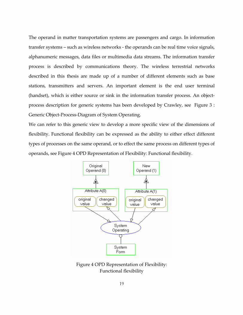
The operand in matter transportation systems are passengers and cargo. In information
transfer systems – such as wireless networks ‐ the operands can be real time voice signals,
alphanumeric messages, data files or multimedia data streams. The information transfer
process is described by communications theory. The wireless terrestrial networks
described in this thesis are made up of a number of different elements such as base
stations, transmitters and servers. An important element is the end user terminal
(handset), which is either source or sink in the information transfer process. An object‐
process description for generic systems has been developed by Crawley, see Figure 3 :
Generic Object‐Process‐Diagram of System Operating.
We can refer to this generic view to develop a more specific view of the dimensions of
flexibility. Functional flexibility can be expressed as the ability to either effect different
types of processes on the same operand, or to effect the same process on different types of
operands, see Figure 4 OPD Representation of Flexibility: Functional flexibility.
Figure 4 OPD Representation of Flexibility: Functional flexibility

20
Figure 5 OPD Representation of Flexibility: Capacity and Performance Flexibility

21
The notion of performance can be understood as the difference between the changed state
and the desired state, capacity is related to the quantity (amount of) operand see Figure
5 OPD Representation of Flexibility: Capacity and Performance Flexibility.
These dimensions would be defined by the range of the Performance and the Capacity
related attributes which are part of the transforming attribute of the primary intent and
the operating attribute of the process. There is another class of attributes which are
“Resource Attributes” (e.g. Cost) , which would set the constraints for the architectural
tradeoff and cost/benefit analysis.
Product flexibility can be achieved by activating dormant features or adding to existing
features to provide enhanced functionality along these dimensions at a later part of
product life cycle.
Why Three Dimensions?
Product flexibility could mean flexibility in multiple features of a product. A rigorous
analysis, which includes quantification of the range of such features, accessing the cost
and value of embedding this range of features would be a complex task.
We used Crawley’s architectural framework [4] to derive three categories of favorable
product “features”. These categories are –

22
Transformation of the beneficial attributes of the primary intent: Almost all products,
transform one or many beneficial attributes. The Transformation process defines the first
category of flexibility dimension. For example
Figure 6 Intent‐Process‐Object Diagram for 2G GSM Network , shows that the primary
intent of enabling outdoor voice conversation is enabled by the process of mobile voice
call. The Transformation process acts on a set of attributes. We can also see them as inputs
to the transformation function.
The second dimension is defined by the volume of these inputs. In the example shown in
Figure 6 Intent‐Process‐Object Diagram for 2G GSM Network , this dimension will drive
the (traditional) voice calls capacity supported by the network. The set of attributes that
are transformed, have a “rate” of transformation.
The third dimension is defined by this rate. In the example shown in
Figure 6 Intent‐Process‐Object Diagram for 2G GSM Network , this dimension can be
characterized how fast the primary intent is transformed (rate of enabling of voice
conversation). This will drive the (traditional) peak calls/second metrics of the network.
We should remember, however, that there could be attributes that are related to the
operation of a product and those could have a set of parallel flexibility dimensions apart
of these three. An example of an operating performance measure might be the Mean
Time Between Failure (MTBF).
Thus the motivation for the classification of the flexibility dimensions is due to two
important reasons:

23
1. Ease of identification of the “features” that would make the product flexible.
2. Ease of quantification of the range of these features.
Figure 6 Intent‐Process‐Object Diagram for 2G GSM Network
The objective of this thesis is to quantify a range of the functional, performance and
capacity attributes which would make the product “flexible” and then analyze the
tradeoff between the resource attributes and the value delivered due to flexibility.
24
The Functional, Capacity and Performance flexibility dimensions are the “results” of a
flexible product. These dimensions can be achieved by Reconfigurability, Platforming
and Extensibility [9]. Some examples of flexibility dimensions with respect to different
industry segments are described in the following sections.
Hardware (Processors)
A processor design optimized for only a particular class of application, leads to the
constraint of meeting needs of only one market segment. There is an uncertainty
associated with how the application scenario, will evolve. Implementing design features
for a flexible feature (e.g. cache architecture), we incur a cost in terms of additional design
effort, complexity and allocation of resources, which detract from traditional performance
metrics (for example it may lead to higher power and die cost ).
By implementing flexible design features which enable customization of applications, by
enabling of an additional on‐chip cache at a later decision point in time we can potentially
maximize the net benefit by meeting new market needs which may translate into a higher
ASP (average selling price) for each unit when the new features are enabled. These
features can be:
Operating Power Supply range changed to support mobile/desktop functionality.
Multi‐Threading enabled for greater CPU performance.
Security features enabled in wireless handsets for premium market segments.
Additional cache enabled for better performance.
Software (Network Applications)

25
A distributed network application can be designed, keeping in mind the functional,
capacity and performance scalability. Such an application could have “hooks” to add a
feature, or increase the application capacity at a later point in time. These features can be
Capacity of the database increased to meet increased capacity needs
Additional servers, with different instances of the application running in a load
sharing mode to increase the performance of the network application.
Additional application features enabled (either on the same server or on different
server).
The software “flexibility” features can be designed and embedded in a product and
activated later based on license agreements (increased capacity or functionality).
Configurability, which is particularly important from the point of view of software
products, can be is perceived as a feature in a product to enable the flexibility dimensions
in the future.
Civil Architecture
The concept of extensibility, as defined by Crawley [4] was to enable a system to be scaled
up significantly in the future or “organically integrate with a larger systems”. For this, he
believes that there should be a “master plan” to have a future map of this extensibility
and the interfaces must be designed with this in mind. Provision for expansion slots for
an additional bedroom or a new barn under the master plan of a house could be example
of this extensibility.
From the context of the dimensions of flexibility, the provision to add an additional
bedroom provides a capacity flexibility and provision to add a new barn provides a
functional flexibility.

26
Transportation
Blended Body Wing architecture presents an excellent example of modular platform
architecture, which enables flexibility [5]. The use of a single flexible platform enables
Boeing to be able to design a system which can be adapted to meet the demands of the
market. Boeing invests large amounts of R&D capital investment, in face of uncertainty (it
can not predict accurately the demand for either type of aircraft ‐ Commercial, Cargo, and
Military, or the quantities of these). By designing a BWB platform as shown in Figure 7
Reusable Components , Boeing can adapt the final mix of products manufactured based
on the actual market demand without the need to design a new aircraft from scratch.
Figure 7 Reusable Components (Source [5]): The blue components – cockpit and wings are common among the whole product family. The green and yellow components are customized, while the grey components are unique for each variant.

27
1.2.2 Assessing Flexibility
The flexibility in each of the dimensions identified in the research effort will be assessed
critically from the point of engineering and management domains. The engineering
domain would include (among others) performance and cost penalty due to embedding
flexibility. Management domain would include analysis of impact of architectural
flexibility on the market competitiveness by a financial evaluation of the optimal
flexibility options.
1.2.2 Embedding Flexibility
The dimensions of flexibility identified in the definition are investigated to a practical
depth to gather further insight in embedding flexibility into products and system
architectures. Some of the aspects that are covered include ‐
Study of performance, capacity and functionality from the context of network based
wireless applications.
Formulation of a general model of the dimensions of flexibility for network based
application.
The overlap of flexibility objective space with the overall objective space. – in other
words what are appropriate functional operating modes of the system and what
performance bandwidths (upper and lower) bounds are appropriate? de Weck has
shown a way to map the Design space to the Objective space using a system model, to
evaluate different architectures [3]. The Flexibility objective space can be mapped to a
subset of this Objective Space, which would necessitate incorporation of a range of

28
design space in the overall flexible architecture, see Figure 8 Flexibility Design and
Objective .
The identification of the flexibility objective space will depend on factors that would
address uncertainties due to dynamic customer needs, technology, corporate strategy,
market conditions, competitive scenario, economic and regulatory policies among other
factors. An example of this space is shown in Figure 1 Flexible Design Objective
Space (Adapted from [1])).
Figure 8 Flexibility Design and Objective Space. Adapted from [6].
1.2.3 Approach
29
1.2.3.1 Methodology
The dimensions of flexibility are explored using the components of a wireless
communication network (PLMN). The analysis is used to formulate a generic framework
of flexibility in Network Application space.
The framework for determining cost of embedding flexibility for a product is established,
based on the quantification of flexible design space as a sub‐set of the overall design
space for the product. The analysis to determine the value of embedding flexibility is then
done using the real options approach. The Black‐Scholes model and the Binomial model
are presented as methods for computing the economics of financial options. These
methods are then applied to computing the value of flexibility options. In order to
determine the value of the underlying asset, which is one of the terms needed for the
valuation of flexibility, two approaches are presented: conjoint analysis and concept
engineering. The bounds of time to expiation are explored. Whenever possible a baseline
system/product with no flexibility embedded in it is used as a reference system. Thus
flexibility is treated as a “real option in a project”, rather than real option on a project.
This requires a reinterpretation of time to expiration. The overall framework, mapping
the design space to the objective space, with respect to the cost and value of flexibility is
shown in Figure 9 Flexibility Framework.

30
Figure 9 Flexibility Framework
Finally, a method is proposed for determining the optimal flexibility design vector and
implementing a chain of real option based flexibility strategy. . This approach is based on
T. Luehrmann’s approach [25] of developing a strategy as a portfolio of, possibly nested,
real options.
1.2.3.2 Structure of Thesis
Chapter 1: Defines the scope and objective of the thesis – Describing, Embedding and
Assessing Flexibility, in product and system architectures with respect to terrestrial
wireless networks and handsets.
Chapter 2 Lists the Literature Reference ‐ publications reviewed and referenced in the
thesis. The main focus here is to highlight the difference between embedding flexibility in
31
products and architectures as “real options in projects” as opposed to the more
commonly known options “on projects” or the purely financial options.
Chapter 3 : Describing Flexibility : Proposes the dimensions of flexibility for wireless
networks and handsets after analyzing the determinants of diffusion in the respective
segments. This treats the outcomes of flexibility, i.e. the ways in which flexibility will
primarily benefit the user or customer. This chapter will not specify how flexibility is
achieved in a product.
Chapter 4: Embedding Flexibility: Develops a generic model, representing most of the
nodes in a wireless network, incorporating the flexibility dimensions identified in
Chapter 3. These dimensions are then formally defined and an architectural framework is
proposed to realize the three dimensions of flexibility from the point of network
applications.
Chapter 5: Valuing Flexibility: Builds a mathematical framework to assessing the value a
flexibility design option using the real option analysis. Traditional real options theory
“on” projects is extended to include building flexibility into products incrementally.
Chapter 6: Assessing Flexibility (Parameters): Lists the methods for determining the
values of the option parameters identified in chapter 5. We will see that finding the value
of the underlying asset and determining volatility are particularly challenging in a
product development environment. This also includes estimating the cost of embedding
flexibility.

32
Chapter 7: Builds the strategy to determine the best flexible design vector based on the
methods and results of the preceding chapters and states the conclusions,
recommendations and future work that can be done to expand the framework proposed
in the thesis.
Thesis Roadmap
The information flow organization of the different chapters of the thesis is shown in
Figure 10 Thesis Roadmap , to organize the thesis and help the reader.
1. Introduction 2. Literature Review
3. Describing Flexibility
4. Embedding Flexibility
5. Valuing Flexibility (Mathematical Framework)
7. Flexibility Strategy and Conclusion
6. Assessing Flexibility (Parameters and Cost)
Figure 10 Thesis Roadmap

33
C h a p t e r 2
Literature Review
2.1 General
Identified as one of the possible research areas in the Architecture Trade Methodology
research initiative [3], the primary research objective of the literature review was in the
area of describing, assessing and embedding flexibility in System Architectures. This
review also includes lecture notes of some of the subjects delivered as part of System
Design and Management coursework and patent reviews to identify distributed
architecture for wireless networks.
2.2 Description of Flexibility
The definition of flexibility as the property of a system that allows it to respond to changes in
its initial objectives and requirements –both in terms of capabilities and attributes‐ occurring after
the system has been fielded[1] was used as a guideline for the analysis of the outcome or as
referred in the thesis as “dimensions” of flexibility. These are also sometimes referred to
as “outcomes” of flexibility. In any case these dimensions regard product or system
functional attributes that are directly perceived by the customer. Other descriptions of
flexibility include – Flexible systems allow owner to adapt operating conditions [7] and the
(flexible system) system will have to evolve in the face of changing environments and expectations

34
[4]. Flexibility is one of the desired “ilities” [34,26] from the perspective of System
Engineering and System Architecture under uncertainties. An analysis of the relationship
of flexibility with extensibility [4,6,9] was also done.
Identification of the primary determinants of diffusion (anything that will cause a
favorable diffusion) for the product, within the market context, was the first step to
establish the probable objective space [3] for flexibility. These determinants are indicator
of the future trends in the industry and thus drive the flexibility dimensions of a product.
This study included analysis of the wireless industry (wireless networks and mobile
handset processors) from the context of Technology S‐Curves [11,36], industry dynamics
[36,18,20] and product diffusion [8,18].Identification of the possible product “features”
that will cause a positive diffusion included review of publicly available information in
the company web sites of the key players in the industry1 and market intelligence data
[11, 8, 31,29].Quantification/Definition of the range of these features(s) for wireless
handset processors was done based on analysis of the market research data.
In general, flexibility is embedded in products and systems to be able to better respond to
new customer preferences or trends, without having to redesign a product from the
ground up.
2.3 Embedding Flexibility
This section answers primarily the question of “how is it done”? Thinking about
embedding flexibility in the sense of modular innovation [10], we can distinguish three
levels of real options, when embedding flexibility in systems or products [9]:
1 Wireless Networks : AT&T , Verizon , Vodafone , British Telecom and Mobinet ; Wireless Handset Processors : Intel , Texas Instruments , Analog Devices , Starcore LLC.

35
- Reserving resources: this means that growth potential is assured by leaving
surface area, volume, excess power, computing bandwidth and so forth unused in
one generation of the product, such that a future product feature may use this
resource, should the option be exercised.
- Designing interfaces: the next step consists in designing interfaces between the
baseline product and the area reserved for the flexible product option. These
interfaces can be mechanical, energetic or informational. Industry standards and
common interface requirements documents (ICDs) significantly facilitate this step.
- Designing the flexible product feature: This next step consists in actually designing
the flexible product feature into the product, while using the resources and
interfaces provided for by the previous design steps.
Finally, the last step of the “embedding flexibility” process is actually implementing the
flexible product feature, which is analogous to actually exercising the real option in the
product. This research included analysis of the architectural details from the context of a
flexible implementation of wireless network applications. This research was largely
based on publicly available data, patent search [32]. Signaling System 7 [37], provided a
good insight of the network protocols. Wireless Network evolution was sufficiently
described in Smith and Collin’s book on the subject [38]. The ITU‐T, ETSI and 3GPP
telecommunication standards were also referred2.
2.4 Assessing Flexibility
2 IS‐41C , IS‐95,IS‐54, IS‐136, GSM‐MAP and 3GPP

36
A study of the different valuation methods ‐ NPV and Real Options, indicated that Real
option is better suited for conditions where there is uncertainty [14,15,16]. A good review
of the real option approaches in the existing literature was found in Adam Borison’s
paper [39]. Some of the approaches that were further investigated, based on the categories
described in [39] –
- Classic [17,33] ‐ the absence of data on replicating portfolio for flexible options
may make this approach impractical. Since flexible product options in innovative
industries are not traded on open security markets it is difficult – and often
impossible – to find a replicating portfolio for assessing the value of a particular,
flexible product feature as a European or American Call Option.
- Subjective [25,19] method uses a subjective assessment of price and volatility of
underlying asset. This approach can be used when this assessment is practically
possible and the existence of the assumption of a replicating portfolio exists. In
absence of this condition, the results would not be accurate.
- Dynamic Programming [17], shows an alternate way of estimating the option
price based on binomial lattice. This falls under the category of “simulation”,
where a set of potential future evolutions is created on the computer and run
against the flexible product architectures.
In order to recommend methods to estimate the option parameters (of the chosen
method), Conjoint [21,22] and Kano [24] analysis were investigated. Conjoint analysis
was found adequate for subjective assessment of the value of the underlying assets,
when used in conjunction to product diffusion data. Kano Analysis [24] provides an
estimate how well the “customer satisfaction” scales with “flexibility”. The basic
37
concept is to double check the dimensions of diffusion identified in the Description
section, to determine whether or not a customer is willing to pay for a scaled of
flexible feature.
The flexibility dimensions (Functionality, Capacity and Performance) are explored to
mathematically convey the relationships between Flexible design space and the
objective space. System Engineering Methods like QFD [30] was studied and
recommended for this transformation. The mathematical notation used to map Design
Space to Objective Space were based on Olivier de Weck’s paper on Architecture
Trade Methodology [3].
The cost of implementing flexible design options for wireless network applications
was determined using the server costing data available of relevant servers on
company website of Sun Microsystems.
Once an optimum design option is defined, assessed and embedded, we reviewed
methods to “nurture” this portfolio .The strategy recommended by Luehrman [25],
where the chosen portfolio is” tracked” to nurture – or populate/develop the fruitful
slots (in his paper, he refers to these as ripe tomatoes) and ignore the unpromising
ones, can be used to nurture the flexibility design options. According to this
framework each option is assessed using two separate metrics,. First, NPVq, which is
the quotient formulation of Net Present Value, which accounts for the value of being
able to defer an investment. The second metric, is the cumulative volatility �*sqrt(t),
which captures both the time to expiration as well as the riskiness of the option. Here
a large volatility is positive due to the asymmetry of possible option value. The value

38
of a flexible design option can never be negative. However, the initial investment to
purchase the real option by reserving resources, designing interfaces or the product
feature itself might be lost.

39
C h a p t e r 3
Describing Flexibility
3.1 Introduction
Flexibility can be understood as the ability of a system or product to support new features
and to perform these at some finite range of operating conditions and capacity levels
during later stages of its lifecycle. The new features can be classified in three important
non orthogonal dimensions from the perspective of wireless network applications and
handsets:
As described in Chapter 1, Functional flexibility can be expressed as the ability to either
effect different types of processes on the same operand, or to effect the same process on
different types of operands, see Figure 4 OPD Representation of Flexibility: Functional
flexibility. From the context of wireless network applications and handsets, this would
map into the ability to perform additional (or a range of) functions.
Capacity flexibility is related to the quantity (amount of) operand, (see Figure 5 OPD
Representation of Flexibility: Capacity and Performance Flexibility )and will be defined
by the Capacity attributes. From the context of wireless network applications and
handsets this would map into (among other features) the ability to handle additional (or a
range of) quantity of interactions.

40
Performance flexibility can be understood as the difference between the changed state
and the desired state and has a ‘rate’ component. This would be defined by the range of
the Performance attribute, see Figure 5 OPD Representation of Flexibility: Capacity and
Performance Flexibility. From the context of wireless network applications and handsets
this would map into (among other features) the ability to handle additional (or a range of)
interaction rate.
Identification of the primary determinants of diffusion (anything that will cause a
favorable diffusion) from the context of product feature, within the market context, is the
first step to establish the probable operating space for flexibility. These determinants are
indicator of the trends in the industry and thus drive the flexibility dimensions of a
product.
Figure 11 Focus of Chapter 3 (adapted from [4])
Focus of Chapter 3

41
The upstream influences in identifying the Needs and Goals for a flexible architecture
were mapped to Crawley’s framework [4] , as shown in Figure 11 Focus of Chapter 3
(adapted from [4]).
It should be noted that “a range of” functions, volume and rate of interactions can be
either more (Forward Flexibility) or less (Backward Flexibility) with reference to the fixed
design.
There are two key steps in this process:
- Identification of the possible product “features” that will cause a positive diffusion.
- Quantification/Definition of the range of these features(s) for a flexible product. This
range will be the objective space for the flexible product.
This analysis is done for Wireless Networks and Wireless Handset processors in the
subsequent sections. The wireless networks are analyzed from a “long term” perspective,
which would be typically 4‐5 years, based on the current trends of network convergence
and upgrade. The wireless handset processors, on the other hand, are analyzed from a
“short term” perspective of 1‐2 years.
Figure 12 Wireless Value Chain
Application Service/Content
ProvidersNetwork OEM’s
Mobile Network Operators
Handset Manufacturers
Component Manufacturers
End Users

42
This analysis was deliberately designed to validate the flexibility dimensions from the
point of long and short term determinants of diffusion in different segments of the same
value chain as shown in Figure 12 Wireless Value Chain.
We were able to identify the possible product “features” that will cause a positive
diffusion for both the cases. Definite quantification/definition of the range of these
features(s) for a flexible product was done for the “short term” case of wireless handset
processors. This was because, in order to define flexibility features with a bounded
uncertainty, we found the current market research data on wireless handset processor
diffusion, adequate (in contrast to similar data on wireless networks). One of the
flexibility feature identified (cache architecture), is used to analyze the value of flexibility
in Chapter 5 (Valuing Flexibility)
Once the determinants of diffusion are identified, these are then classified based on
similar attributes to derive the flexibility dimensions that would enable the product(s) to
operate in a finite range (flexible objective space) in the overall objective space as shown
in Figure 8 Flexibility Design and Objective Space. Adapted from [6].

43
3.2 The Wireless Network
The primary determinants of diffusion for the Wireless Networks are very important to
establish the probable operating space for flexibility. These determinants would be an
indicator of the trends in the industry and thus drive the flexibility dimensions. In this
section, the background of the Wireless Networks is explored, to identify these
dimensions.
3.2.1 Network Evolution
The overall reference of performance (and from the context of the, flexibility dimensions)
of the wireless networks has historically been on two key areas‐ Call Capacity and Data
rate. Though the apparent indicator of increased performance in the evolution of the 2G
networks has been the data rate (9.6 Kbps to 2 Mbps), the carriers are more interested in
the capacity scaling that the evolving networks provide (from tens to hundreds of users
per cell).
The qualitative performance scale for wire line network evolution is based on cost per
subscriber (including the fixed infrastructure cost and variable operating costs). Lower
the cost, higher is the relative position in this scale. The Technology S‐Curves [11]
showing the evolution of the wireless networks from 1G to 2G to 3G networks is shown
in Figure 13 Wireless and Wire line Network Evolution in North America.
The wireless and wire line S curves have been superimposed to give us an idea of the
timeline of evolution and a qualitative view of the comparative performance.

44
Figure 13 Wireless and Wire line Network
Evolution in North America
Today wireless networks can be set up at fraction of the costs of traditional wireline
networks. This is one of the reasons the third world countries are adopting the wireless
networks directly (skipping the wireline evolution phase).
3.2.2 Evolution of Standards

45
The Wireless Industry is divided by three dominant standards – GSM, TDMA and
CDMA3. GSM has evolved as a standard of choice based on overwhelming adoption by
users throughout the world as compared to the other two standards [13].
0
200,000,000
400,000,000
600,000,000
800,000,000
1,000,000,000
1,200,000,000
1992 1993 1994 1995 1996 1997 1998 1999 2000 2001 2002 2003
TDMACDMAGSM
Figure 14 Diffusion for TDMA, CDMA and GSM. (Source: [12])
The diffusion curve of GSM is steep due to the Network Effects and positive feedback
due to widespread adoption throughout the world as shown in Figure 14 Diffusion for
TDMA, CDMA and GSM. (Source: [12]). This diffusion curve is derived using the Lotka
Volterra model, which is a simple model of predator‐prey interactions.
Number of Subscribers
Year
3 See Appendix A for an overview of GSM , TDMA and CDMA frequency allocations and modulation schemes

46
TDMA and GSM are both based on similar concept of Time division Multiplexing and
have joined hands in the “standard tipping” war against CDMA which is considered to
be technically superior to TDMA or GSM. This has helped in increasing the installed base
of the TDM camp. The global 3G standards are based on CDMA technology. CDMA has
higher spectrum efficiency as compared to TDM (TDMA and GSM). Dynamic bandwidth
allocation provides flexibility in the maximum number of users supported per cell in
CDMA networks; this number is fixed based on the total timeslots in TDMA and GSM
networks. In TDM networks, adjacent cell interference is a common problem, in cases
where the cell sizes are very small and the carriers have limited bandwidths. This
problem is not present in CDMA networks, therefore modification of the existing cell
structure is easier, giving flexibility to the network operators to modify or expand their
networks.
3.2.3 Europe Vs N America in 2G Standard Evolution
ETSI (European Telecommunication Standards Institute) organized the GSM standard, at
the Pan‐European level. Europe had faced lot of interoperability problems due the
multiple Analog Standards that existed before the 2G migration was decided and was
motivated to adopt a common standard to mitigate the interoperability problem in the 2G
networks. European Wireless Operators strategy to capture value was to build the
installed base based on a consensus standard (GSM).
America on the other hand had just one Analog Standard (AMPS) – and evolved to the
2G wireless networks under two paths CDMA (IS‐95) and TDMA (IS‐136). The American

47
wireless industry followed the strategy of “Let the Market decide the Standard” strategy.
CDMA did not catch on in Europe because it had not developed fully enough to beat
GSM during the selection period that ETSI had set.
3.2.4 3G Network Evolution
3.2.4.1 CDMA –Technological Edge
The Code Division Multiple Access (CDMA) technology was developed by Qualcomm.
CDMA is widely considered a better technology as compared to the Time Division
Multiplexing technology used by GSM and TDMA because of its superior spectral
efficiency and lower installation and equipment costs. The Global wireless standards that
are proposed by G3G (Global 3 G Standard Committee) is WDCMA – which is based on
CDMA technology.
Strategic Alignment [18] of Primary Producers (TDMA & GSM)
In the Evolution to 3G networks, the TDMA and GSM standards aligned to have similar upgrade paths via GPRS, EDGE and WDCDMA ( Figure 15 Evolution Paths of TDMA, GSM and CDMA) . This alignment was
strategically very important, wherein though the operators would be licensing some
portions of the CDMA technology, they could resist the effort of Qualcomm to make
CDMA2000 as the worldwide standard, where Qualcomm would have a substantially
greater share of the overall value and a possible Winner Takes it all situation. The
standard war was resolved after many publicized rounds of confrontations.

Figure 15 Evolution Paths of TDMA, GSM and
CDMA
Strategic Alignment of Primary Producers (CDMA & GSM)
Qualcomm and Ericsson (Dominant Player in the GSM Market) had an Intellectual
Property deal in 1999, facilitated by the OHG (Operators Harmonization Group). This
resulted in the convergence of three paths of CDMA evolution (cdma 2000, WDCDMA
and TDD) TDD standards are not yet finalized. WDCDMA was aligned with the GSM
and TDMA evolution path.
This aligned the evolution path of CDMA, TDMA and GSM. As part of the agreement,
the companies committed to licensing their essential patents for a single CDMA standard,
removing all intellectual property restrictions that currently were in force. Ericsson
purchased Qualcomm’s terrestrial CDMA wireless infrastructure business, including its
research and development facilities in San Diego and Boulder, Colorado. In 2001
Qualcomm and Nokia had a similar cross license agreement.
GSMWDCDMAGPRS EDGE
CDMA Cdma2000IS95A 1xRTT
GPRS WDCDMAEDGETDMA
48

49
3.2.5 The Future
Due to the efforts of the different standards committee’s – the overall wireless industry
seems to have tipped towards the CDMA standard. It is interesting to note that the GSM
camp would still retain the value it had created due to the early market penetration,
based on strategic alignment with a technically superior standard.
This way, it will be able to use its vast installed base and complimentary assets, without
the risk of defection in the future. From the context of flexibility we will analyze the
wireless network from the context of a single converged standard.
3.3 Diffusion in the Wireless Industry
As mentioned earlier, the primary determinants of diffusion are very important to
establish the probable objective space for flexibility. These determinants would be an
indicator of the trends in the industry and thus drive the flexibility dimensions.
The Diffusion in the Wireless Industry can be perceived in at least two dimensions. The
first dimension is the traditional voice service, where the industry is currently wooing the
“Late Majority”. The Determinant for diffusion in this dimension is the support for
increased number of subscribers. Wireless network operators want to ensure that they
can continue to support their existing subscribers (and continue their subscriber base
expansion), before introducing the high bandwidth value added services. From the point
of view of the Network operators, Cost of deployment and Spectrum allocation would
also guide to a big extent the expansion of the networks.

50
The second dimension is Value Added Applications, where the wireless industry is in the
process of crossing the chasm between the Early Adopters and Early Majority. A key
Determinant for diffusion for the wireless industry in this dimension, is the subscriber’s
need for assessing value added data, while on move (apart from the traditional voice
connectivity).Value added data includes localized and personalized data, high
bandwidth entertainment data, among others.
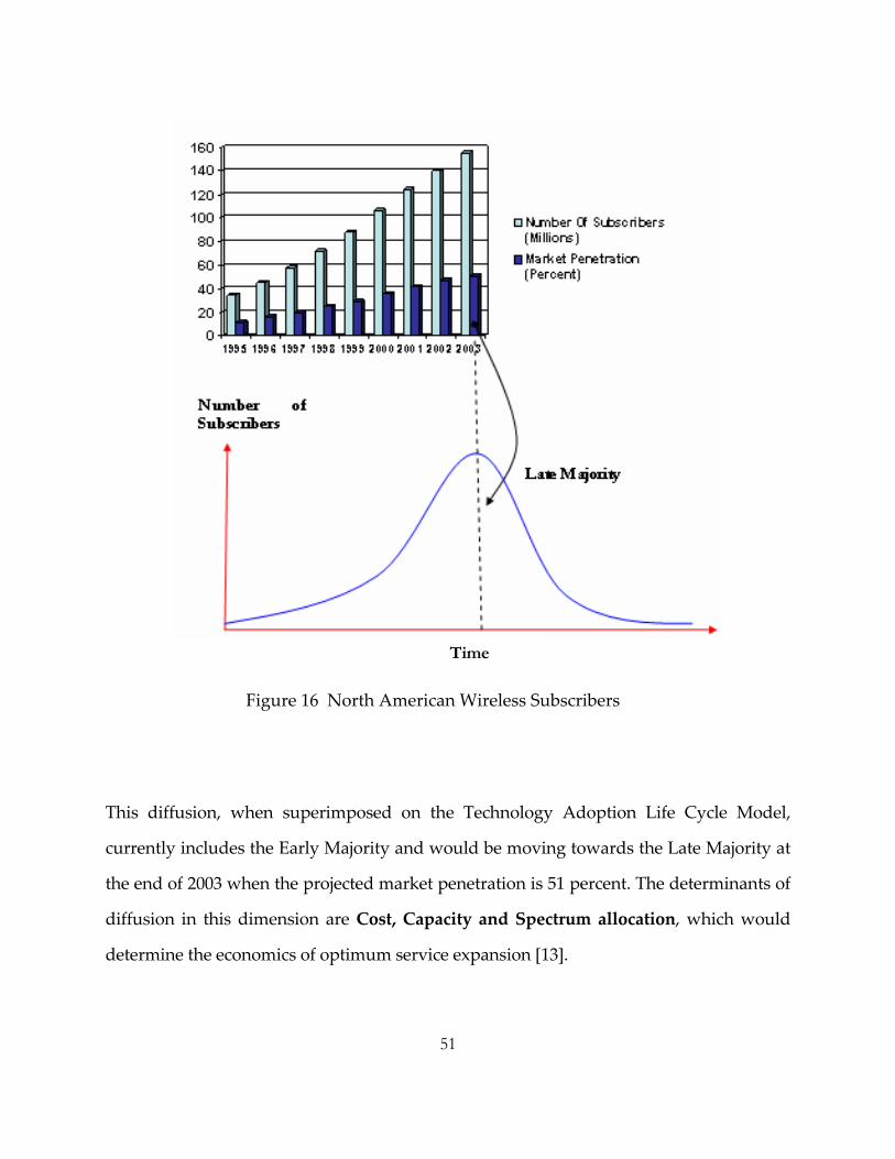
3.3.1 The Voice Dimension ‐ Late Majority
Total number of wireless subscribers has grown at a steady rate since 1995(Figure 16
North American Wireless Subscribers) shows the number of subscribers in North
America.
51
Figure 16 North American Wireless Subscribers
This diffusion, when superimposed on the Technology Adoption Life Cycle Model,
currently includes the Early Majority and would be moving towards the Late Majority at
the end of 2003 when the projected market penetration is 51 percent. The determinants of
diffusion in this dimension are Cost, Capacity and Spectrum allocation, which would
determine the economics of optimum service expansion [13].
Time

52
3.3.2 Cost
The Network operators are very sensitive about the cost of upgrading their networks,
where the projected capacity crunch is about 2 years away, based on the current
infrastructure. The cost would have a specific impact on the Diffusion of a particular type
of network (CDMA, TDMA, and GSM). CDMA has a higher initial cost, which would
make the GSM, TDMA upgrade option attractive to the carriers in the near term. This
makes it imperative to calculate the cost and value of embedding a flexible design option.
The cost is part of the “resource attribute of transferring” as shown in Figure 5 OPD
Representation of Flexibility: Capacity and Performance Flexibility. The methods to
calculate this cost and value are explored in Chapter 5 and Chapter 6.
3.3.3 Capacity
The wireless carriers (network operators) want to ensure that they can continue to
support their existing subscribers (and continue their subscriber base expansion), before
introducing the high bandwidth value added services. The voice service is a proven
revenue source – data is not yet. This is an important determinant that would affect the
diffusion of wireless network as a whole, where the subscribers are demanding or would
demand value added applications (Market Demand).The network capacity in terms of
total number of subscribers will directly map into the Capacity dimension of flexibility
and is part of the “capacity attribute of transferring” shown in Figure 5 OPD
Representation of Flexibility: Capacity and Performance Flexibility. There is a dimension
of performance, which will be related to the peak call rate supported by the network,

53
which is also part of the overall network capacity, and will be part of the “performance
attribute of transferring”.
3.3.4 Spectrum
The current spectrum restriction per carrier (45 MHz) in particular market limits the
market penetration – and thus diffusion in that market. This is therefore part of the
“resource attribute of transferring” as shown in Figure 5 OPD Representation of
Flexibility: Capacity and Performance Flexibility.
3.3.5 Value Added Applications
The value added applications would increase and sustain the subscriber’s base.
Some of the applications facilitate increased air time usage, increasing the ARPU
(Average Revenue per User).
3.3.5.1 Applications – driving the future
With the industry still looking for the “Killer Application” and innovative startups
coming with customized value added applications, to help the network operators capture
and retain new market segments once the Chasm [8] between early adopters and early
majority is crossed.
Some of the value added applications like Wireless Messaging have expanded the
subscriber base to a totally new market segment e.g. the school going teenage segment.
These applications are extremely popular in Europe and Asia and are catching up in
popularity in the US, where network interoperability issues had prevented the diffusion

54
of these applications in the past (which have been resolved now). These applications will
map into the functional dimension of flexibility.

55
3.4 Wireless Handset Processors
The next generation wireless handsets are growing increasingly complex. The existing
battery technologies have not been able to keep in pace with the advancement of circuit
technology and power demand of these handsets. The current trend to temporarily solve
this problem is to make the handset more “fuel efficient” using system level energy
conservation methodologies [28]. It is predicted that a 5X improvement in battery life is
achievable by carefully applying these methodologies.
A visible trend in the market is the evolution of wireless PDA’s and camera phones. The
convergence of the PDA’s with cell phones is leading to increased power demands for
these complex handheld devices There is also a trend of migration of increasingly
complex PC based office and multimedia applications in these handheld devices.
There is a high possibility of increasingly complex mobile applications, becoming popular
in the future. The system level energy conservation methodologies involving dynamic
frequency and voltage management, pioneered by Intel, might not be sufficient to keep
up to the demands of such applications in long run. Strategic alliances between DSP and
RISC houses (as seen by the recent alliance between Intel and Analog devices for PXA
800F which targets the GSM/GPRS data application segment) are indicators of
technological trends to address this issue.
In this section, the determinants of diffusion for low power and high performance
processors in the wireless segment are explored after analyzing the whole wireless
application value chain. This analysis is used to predict the optimal features of such
processors (for the next few years), which is critical for early market penetration in a

56
segment that is predicted to be larger than the desktop segment in a few years. These
features would be analyzed from the three flexibility dimensions – Functionality,
Performance and Capacity.
3.5 The Value Chain
The value chain for wireless applications is shown in Figure 12 Wireless Value Chain.
The primary concern of the Mobile Network Operator’s (MNO’s) today is voice service,
which has the lion’s share of the current MNO revenues.
3.6 End Users
The end user adoption of the wireless applications has not been consistent across the
globe. There are distinct geographical patterns that have emerged, like the adoption of
2.5/3G applications in Japan (MOVA/FOMA), SMS applications in Europe and Asia and a
lack of adoption of either of these applications in North America.
3.7 Applications Service/ Content Providers
Figure 12 Wireless Value Chain, shows Application Service providers parallel to the
MNO’s in the overall value chain. The Application Service / Content Providers can be
also depicted downstream in the value chain after the MNO’s. Since the voice service,
which is of primary importance in the overall value chain, is directly provided by the
MNO’s, the parallel representation is chosen for this report.
There is however, a considerable influence of the MNO’s on the value proposition of the
Application Service / Content Providers. For example, interoperability was a key issue
57
that limited the diffusion of SMS applications in US. Similar issues (which are discussed
in the next section) could influence the adoption/diffusion of future wireless applications.
In this section, wide categories of future wireless applications are explored. These
applications are currently in different stages of development. in companies all across the
globe.
3.7.1 Security Applications
These applications would enable remote access of the mobile computing devices, if the
device is lost or stolen. If the device is stolen, it can be activated remotely to “report”
mode where it transmits its location to the owner (source: Intel.com)
If the device is lost, the hard drive can be remotely locked to protect critical data. The
device can be recovered by activating the “report” mode.
Currently the users of complex mobile computing devices prefer to turn these devices off
to conserve battery power. The security applications would need these devices to be
“always on” in an analogous mode of Cell Phones, which are also always on to receive
data on the control channel (e.g. handoff, incoming call etc).These advanced devices
would operate in semi‐standby mode and would be location aware.
This would put substantially higher standby power requirement, – a demand that has to
be fulfilled partly by a low power monitoring core loop, typically running on a DSP.
3.7.2 Gaming Applications

58
Currently online games can only be played with a PC, although the 128‐bit consoles
were all developed with some kind of internet connectivity in mind. This market,
currently generating revenues of about $152.2 million annually, is affected by the slow
rate of broadband adoption [31].
Like online gaming, wireless gaming has the attention of many in the industry, and
could cause significant diffusion of wireless data services due to huge network effects.
At the present time, however, most wireless games have primitive graphics.
Introduction of better mobile computing processors will make the wireless graphics
comparable to the PC consoles. These applications would be very computation
intensive and would be a driver of reduced power consumption.
The battery life of basic PDAs with a monochrome screen can be weeks, but as soon as
the devices are more sophisticated, with color display and wireless connectivity, battery
life can be as short as two or three hours.
Processor power consumption typically accounts for approximately 7 percent to 10
percent of total notebook power consumption, while the LCD, chipset, and graphics
consume the most power on a percentage basis at approximately 30 percent, 13 percent
and 10 percent, respectively4. This data indicates that in the segment of gaming
applications, low power CPU would have to be complimented with efficient displays
and system level power optimization techniques.
3.7.3 Location Applications
4 source : Intel.com

59
The next generation location applications would involve “digital solicitation”, where an
individual’s computing devices would represent his or her interests and would
seamlessly interact with the environment, looking for promotions and negotiating offers.
An example scenario is that if you are in the market for a particular type of digital
camera, you input your preferences in your wireless computing device, with the price
you are wiling to pay. When you go to a mall – your device interacts with the retail outlet
“promotional computer” and informs you if such a camera is available.
These applications need a lot of background computation, increased drain power and
thus need for low power computation.
3.7.4 Multimedia Applications
There is a big potential of video/news on demand applications, which would be very
popular with business travelers. One could download a movie in his or her laptop or the
latest NBC news clip in his of her handheld computing device. These multimedia
applications are again computation intensive causing a demand for efficient, low power
processors.
Streaming Multimedia applications like video conferencing and broadcast applications
like picture sharing would also need low power multimedia decoding, typically suited
for a DSP processor.
Mobile Network Operators
60
Evolution Path
The evolution path of the TDMA, CDMA and GSM networks is
shown in
Figure 15 Evolution Paths of TDMA, GSM and CDMA. In US, Wireless Networks based
on all three standards, have national footprints.
There are two possible Networks upgrade paths – first is a direct 2.5G‐3G upgrade, which
costs less than the 2G‐2.5G‐3G upgrade. Since the recent downturn of the telecom
industry, the MNO’s have delayed their 3G network deployment and have chosen a 2G‐
2.5G network upgrade as a stop‐gap solution, which will cost considerably less than 2G‐
3G upgrade and would start the diffusion of low bandwidth data applications.
As a case study, there are two known 3G network deployment in Europe – Mobikom in
Austria and 3 in UK and Italy. Both the networks are grossly underutilized and the
operators are now offering 3G connection at the same price (or even less as part of
promotions) of the conventional 2/2.5 G networks.
Learning by the example of European MNO’s, it is likely that the North American MNO’s
delay their 3G rollout plan. This was indicated by AT&T’s announcement to delay their
3G rollout and announcement of their network upgrade to 2.5G (GPRS) last year. 2.5G
services are widely available in the US today.
As mentioned earlier, the primary concern of the Mobile Network Operator (MNO) today
is the voice service, which has the lion’s share of the current MNO revenues. The data
applications would be used as a differentiating feature for a few years, to reduce churn,

61
rather than a dominant revenue source. Interoperability issues like inter‐network GPRS
roaming, has to be resolved, and can effect the diffusion of data applications.
Bundling Strategy
There is a trend in European MNO’s (Vodafone and Orange), to have strategic alliance
with relatively unknown handset manufacturers (in the current market), which enables
them to command a lower price and thus less handset subsidization costs. An example is
Similar trends are likely for North American MNO’s, making it imperative to identify
these handset manufacturers (from the point of view of design wins of mobile handset
processors).
Data Rate
The data rated supported by currently deployed GPRS solutions, as evaluated by Intel, is
53.6 Kbps (source : Intel.com). 1xRTT supports data rate of 40‐70 Kbps. Thus applications
that can be deployed on this bandwidth are likely to initiate the diffusion of data
applications in the wireless networks, in next few years.
Handset Manufacturers
The Asian wireless market had around 100 million 2.5g handsets last year which is
predicted to ramp down to 5 million handsets by the end of 2007. 3G handsets are
expected to ramp up from 2.5 million in 2003 to 128 million in 2006 [29] see Figure 17 Asia
Pacific Handset Sales.
The 2.5G and 3G handsets are predicted to change their dominant status sometime in
2005. NEC, which is the leading handset vendor, has an emphasis on 2.5 G handsets.

62
Figure 17 Asia Pacific Handset Sales (Data source: [29])
There is a very high likelihood that similar trends (2.5G handsets dominating the market
for the next few years) is followed in the European and North American markets, where
3G network deployments is not as extensive as in Asia.
0
20
40
60
80
100
120
140
2002 2003 2004 2005 2006
Year
Asia Pacific Handset Sales(Millions)
2G (GSM)2.5G (GPRS)3G(WDCDMA)
3.8 Processor Manufacturers
As indicated by the application trends, the performance of a processor used in handheld
platforms needs to be optimized for both dynamic power consumption as well as standby
power consumption. The definition of standby operations in wireless platforms includes
monitoring of control channels.

63
Smaller device geometries result in greater packing densities and lower device switching
capacitance which is proportional linearly to the device capacitance. This increases the
standby current with every process generation. The handset segment, which typically
relies on smaller geometry than desktop segment, will impose a stringent power
requirement on desktop processor segment players like Intel.
The wireless application segment is a unique mix of the traditional DSP applications and
Desktop applications. , shows the two distinct feature migration path, where dominant
players in the desktop application segment, are focusing their efforts in power reduction.
The traditional DSP houses are focusing their efforts in making their processors
competent to handle complex interfaces (including user interfaces).
Figure 18 Migration Strategy of key players in the
wireless processor segment.

64
3.9 Approach 1 – Reduce the power
With increasingly complex mobile applications becoming popular, this approach relies on
usage of design optimization methodologies to reduce the power demand. It is predicted
that a 5X reduction in power consumption is achievable by carefully applying these
methodologies. Intel’s Dynamic Frequency Management (DFM) and Dynamic Voltage
Management (DVM), has been able to reduce power consumption in the Laptop
Segment. Incorporating these features in their Personal Internet Client (PCA) architecture
is also part of this effort.
Intel has also augmented the system level power management with strategic alliance with
Analog Devices, a leader in the DSP segment. Micro Signal Architecture, Jointly
developed by Intel and Analog Devices, incorporates the system level power
management, GSM/GPRS stack on DSP, Xscale processor and Flash in a singe chip.
3.10 Approach 2 – Enhance Interface Complexity
In this approach, the traditional DSP vendors have enhanced their offering by
augmenting a low power RISC based I/O processor or an ASIC. TI has followed the
System on Chip model by augmenting RISC with their DSP cores for their OMAPTM
Architecture. Starcore has similar model for augmenting their DSP core with a RISC
based I/O core as their solutions targeted for SOC segment.

65
The Future
Based on the analysis of the Wireless Application value chain from the context of
evolution of wireless networks and diffusion of wireless handsets in the US Markets in
the next few years, we can conclude that –
‐ It is more likely that the MNO’s in US would follow a (2G ‐ 2.5G – 3G) network
upgrade path, than a (2G – 3G)upgrade path.
‐ The 2.5 G data rates are in the range of traditional 56Kbps dialup connection (GPRS
data rates of 53.6 Kbps, and 1XRTT data rates of 40‐70 Kbps).
‐ Interoperability issues are unlikely in the diffusion of data applications as these
applications will be TCP/IP based. This will provide substantial network effects.
Issues like GPRS Roaming have to be resolved to realize the full potential of data
applications.
Determinants of Diffusion
‐ With a bandwidth of around 56 Kbps, the future applications (described in the
Application Service Provider section) should be individually assessed for their
practical field requirements and these requirements should be formally translated to
technical specifications using tools like Quality Function Deployment [1674]. A
detailed requirement analysis is beyond the scope of this thesis , but a representative
subset of the relevant requirements for near‐term diffusion are –

66
o Efficient Low bandwidth multimedia streaming algorithms should be
developed by the processor manufacturers.
o Evaluation and Optimization of low bandwidth digital video codec like H.264
(H.26L), should be performed for mobile handset processors. Microsoft and
Nokia’s support to the standard and absence of Intellectual Property issues
may cause a rapid diffusion of this standard.
o Existing processor architecture can be optimized for better performance for low
bandwidth codecs.
o Audio only streaming applications are suited for the identified 56Kbps
bandwidth. Applications for downloading and playing MP3 would necessitate
optimized MP3 decoder implementation for the handsets
o Real – time multimedia applications like video conferencing could be
augmented by relatively lower bandwidth non‐real time applications like
picture sharing using compression protocols like JPEG‐2000.
o High bandwidth codec like MPEG4 is the likely option for 3G bandwidths and
thus the optimization of processor performance for MPEG 4 should be in the
logical roadmap for the processor vendors.
From the context of wireless handset processors, all these requirements fall in the
category of performance optimization. The performance of a processor, with respect to a
particular application (like digital video codec) is usually represented in terms of number
of clocks cycles expended. The driver of performance flexibility can be determined by the
contributors of these cycles. Size of the on‐chip cache, for example is one of the drivers of
the performance. This is because; cache misses (especially instruction cache) cause a
significant amount overhead, which can be reduced by increasing the size of the on‐chip

67
cache. Flexibility analysis, as described in this thesis, can be used to determine the
optimum size of this cache, which could be relatively small for still – picture based
applications (based on JPEG) and has to be relatively large for high bandwidth digital
video codecs (like MPEG).
Conclusion
The study of wireless networks shows that in the future, the diffusion for wireless
networks would continue to be guided by value added applications, within the Cost,
Capacity and Bandwidth Framework. The value added services would be used by the
wireless network operators to reduce churn. These services would determine the new
Performance criteria in the Wireless Industry S Curve – extending the current S‐Curve,
which is in the maturity stage. With respect to wireless networks, it was seen that:
‐ Cost, Capacity, Bandwidth and Value Added Services (VAS) are indicator of the trends
in the industry and thus would drive the flexibility dimensions. These tends would give
rise to a mathematical volatility model, which has to be assessed to calculate the value of
embedding flexibility.
‐ The Network Capacity will drive the Capacity dimension of flexibility.
‐ Spectrum allocation and Cost are the resource attributes that would define the
constraints
‐ The applications (VAS) will drive the Functionality dimension of flexibility.
68
The study of wireless handset processors indicated that in next one or two years, low
bandwidth (56Kbps) applications would drive the diffusion. Performance optimization of
the processors, with respect to the computationally intensive cores (e.g. streaming digital
video codec like H.264) of these applications will drive the performance dimension of
flexibility for the handset processors.
In the original definition of the non orthogonal dimensions of flexibility were defined as:
Functional flexibility can be expressed as the ability to either affect different types of
processes on the same operand, or to affect the same process on different types of
operands, see Figure 4 OPD Representation of Flexibility: Functional flexibility. From the
context of wireless network applications and handsets, this would map into the ability to
perform additional (or a range of) functions.
Capacity flexibility is related to the quantity (amount of) operand see Figure 5 OPD
Representation of Flexibility: Capacity and Performance Flexibility, and will be defined
by the Capacity attribute of transferring .From the context of wireless network
applications and handsets this would map into (among other features) the ability to
handle additional (or a range of) quantity of interactions.
Performance flexibility can be understood as the difference between the changed state
and the desired state and has a ‘rate’ component. This would be defined by the range of
the Performance attribute of transferring, see Figure 5 OPD Representation of Flexibility:

69
Capacity and Performance Flexibility . From the context of wireless network applications
and handsets this would map into (among other features) the ability to handle additional
(or a range of) interaction rate.
Critical analysis of Wireless Networks and Wireless handset processors indicate that all
the short and long term determinants of diffusion can be represented along these
dimensions. This analysis shed light on the case of “Forward Flexibility” where the
objective space identified was “in addition” to the existing operating space (e.g. higher
processor performance and network capacity).
There are cases in the industry where “Backward Flexibility” strategies have been
successfully implemented, to capture the lower end of the existing market (e.g. Intel’s
Celeron Processor). These strategies are feasible when there is low or negligible
incremental production penalty for a flexible product.
The classification of the individual features in these categories (Functionality, Capacity
and Performance) would enable us to perform a three dimensional trade‐off analysis
along these dimensions, with the resource constraints, and access the value delivered due
to flexibility.
In the next chapter, we will explore a specific method to embed flexibility (from the
context of wireless network) by building a generic model that could be used to represent
most of the nodes in a wireless network, incorporating capacity, performance and
functional flexibility.

70
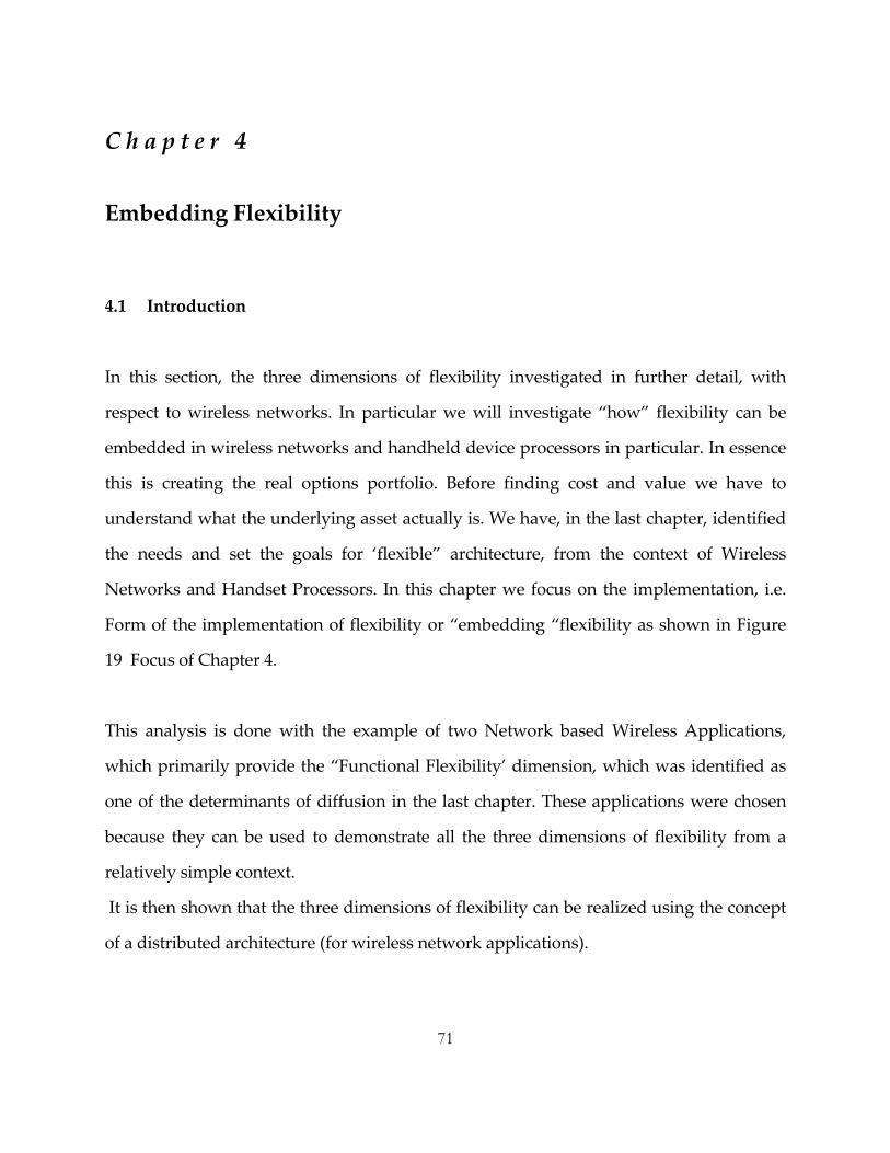
71
C h a p t e r 4
Embedding Flexibility
4.1 Introduction
In this section, the three dimensions of flexibility investigated in further detail, with
respect to wireless networks. In particular we will investigate “how” flexibility can be
embedded in wireless networks and handheld device processors in particular. In essence
this is creating the real options portfolio. Before finding cost and value we have to
understand what the underlying asset actually is. We have, in the last chapter, identified
the needs and set the goals for ‘flexible” architecture, from the context of Wireless
Networks and Handset Processors. In this chapter we focus on the implementation, i.e.
Form of the implementation of flexibility or “embedding “flexibility as shown in Figure
19 Focus of Chapter 4.
This analysis is done with the example of two Network based Wireless Applications,
which primarily provide the “Functional Flexibility’ dimension, which was identified as
one of the determinants of diffusion in the last chapter. These applications were chosen
because they can be used to demonstrate all the three dimensions of flexibility from a
relatively simple context.
It is then shown that the three dimensions of flexibility can be realized using the concept
of a distributed architecture (for wireless network applications).

72
Figure 19 Focus of Chapter 4 (adapted from [4])
Focus of Chapter 4
4.2 Functional Context
The basic functional context of the different nodes in the wireless network is to interact
with each other using defined protocols and perform the required functions. There is a
separate class of applications which passively monitor these interactions and enable value
added services – e.g. Monitoring the network and providing feedback on re‐configuration
(e.g. add more voice trunks on the congested routes) .One of the commercial applications
is to detect international roamers and send customized messages (like exchange rate –
Local weather forecast etc).Our study of flexibility will start with this context and the

73
generic model developed would be expanded to represent all the nodes in a wireless
network.
A brief overview of the architecture of wireless networks and description of the nodes is
provided in the next section.

74
4.3 Network Architecture
A simplified form of the wireless network is shown in Figure 20 Simplified (2G) Wireless
Network
Figure 20 Simplified (2G) Wireless Network
Wireless Network
HLR
BTS BSC MSC/VLR WAP Gateway
SMSC
Network Interface
Client Machines

75
Cell – is a geographical unit with a dedicated scheme of RF interaction with a wireless
user. For GSM and TDMA networks, the adjacent cells have different operating
frequencies. For CDMA networks they have a different code. Cells are typically
visualized as hexagonal, but in actual practice my be of any arbitrary shape based on the
desired coverage location (e.g. Highway) or call density (e.g. NYSE). The two key
components of RF planning are the call volume (based on BTS‐BSC capacity) and
geographical extent of desired coverage. Networks are not designed based on only the
peak call volume as it would lead to underutilization of the resources. The network
design is usually based on the average and peak call volume in a cell, within the expected
quality of service.
BTS – is the base station that provides the RF connection with the handset. It is a
transreceiver. There is typically one BTS for a Cell.
BSC – is the bas station controller, having access to multiple BTS. In some networks the
Base stations are directly connected to the switch.
MSC – is the Mobile switching center – which has access to multiple BTS and performs
the switching function of a call and “hand‐offs” between BSC’s or between switches (if a
user roams to a cell covered by a different switch.
HLR – Home Location Register is a database server that has subscriber information.
There are other servers in the networks (not shown in the figure) e.g. EIR for Equipment
Identification and authentication, VLR for visitor (roamers) data.

76
SMSC ‐ The SMSC is the Short Message Service Center and interfaces with the internet
using multiple schemes – one of them shown in the figure uses a Network interface
server to interact with the users through internet (e.g. WEB based SMS).
The Protocols/Standards
Within a wireless networks, there are two categories of standards
Access Standards for example CDMA (IS‐95) TDMA (IS‐54,136), and
Network Standards5 for example (BSC ‐ MSC (Proprietary, IS‐631),
and MSC to MSC, VLR, HLR, SMSC standard (GSM‐MAP, IS‐41,
ISUP, TCAP). Modular Innovation [10] is common in the Network
standards (Additions to ISUP, TCAP and upgrade of IS‐41 from IS‐41
B to IS‐41C). The latest upgrade to 2.5 G networks in GSM‐MAP,
involved adding of two additional network nodes (GGSN and
SGSN) and upgrading the GSM‐MAP standard (equivalent of IS‐41
for CDMA/TDMA) , as part of the GPRS evolution as shown in
Figure 15 Evolution Paths of TDMA, GSM and CDMA.
4.4 The Dimensions
The application platform architecture used of our analysis, which can be used to
represent the architecture of any of the nodes that are described in the preceding section,
5 Access standards define the interface and protocols between the wireless handset and the wireless network. Network standards define the interface and protocols between the different nodes in a network.
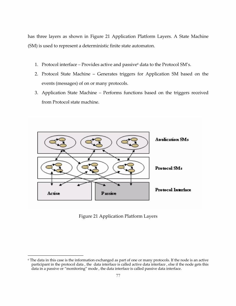
77
has three layers as shown in Figure 21 Application Platform Layers. A State Machine
(SM) is used to represent a deterministic finite state automaton.
1. Protocol interface – Provides active and passive6 data to the Protocol SM’s.
2. Protocol State Machine – Generates triggers for Application SM based on the
events (messages) of on or many protocols.
3. Application State Machine – Performs functions based on the triggers received
from Protocol state machine.
Figure 21 Application Platform Layers
6 The data in this case is the information exchanged as part of one or many protocols. If the node is an active participant in the protocol data , the data interface is called active data interface , else if the node gets this data in a passive or “monitoring” mode , the data interface is called passive data interface.

78
An application state machine can be visualized a standalone application doing a specific
task. There would be specialized interfaces to these applications not shown in the
diagram – like voice trunks in case of switches. We would include these interfaces in our
generic description of systems in the next section.
Another example of a point solution can be “send e‐mail to the charging network with
call details for all abnormally terminated calls”
This configuration can be used to this platform to function as a MSC, HLR, VLR, EIR, and
Application server , which were described in the previous sections.
4.5 The State Machines
In Figure 21 Application Platform Layers, we can theoretically extend the functional
flexibility of the platform using one consolidated state machine that takes care of ALL
possible application scenarios and ALL possible protocols. The two levels of state
machine mitigates some of the issues that would be associated with a single state
machine implementation ‐
Complexity: there are too many input events for a consolidated SM, which is a union of
all protocol events e.g.
N = (ANSI ISUP Events) U (ITU‐ISUP Events) U (MAP Events) …… U (IS634 Events)
If the total states is in the order of N. Total Number of Handlers to be implemented = N2
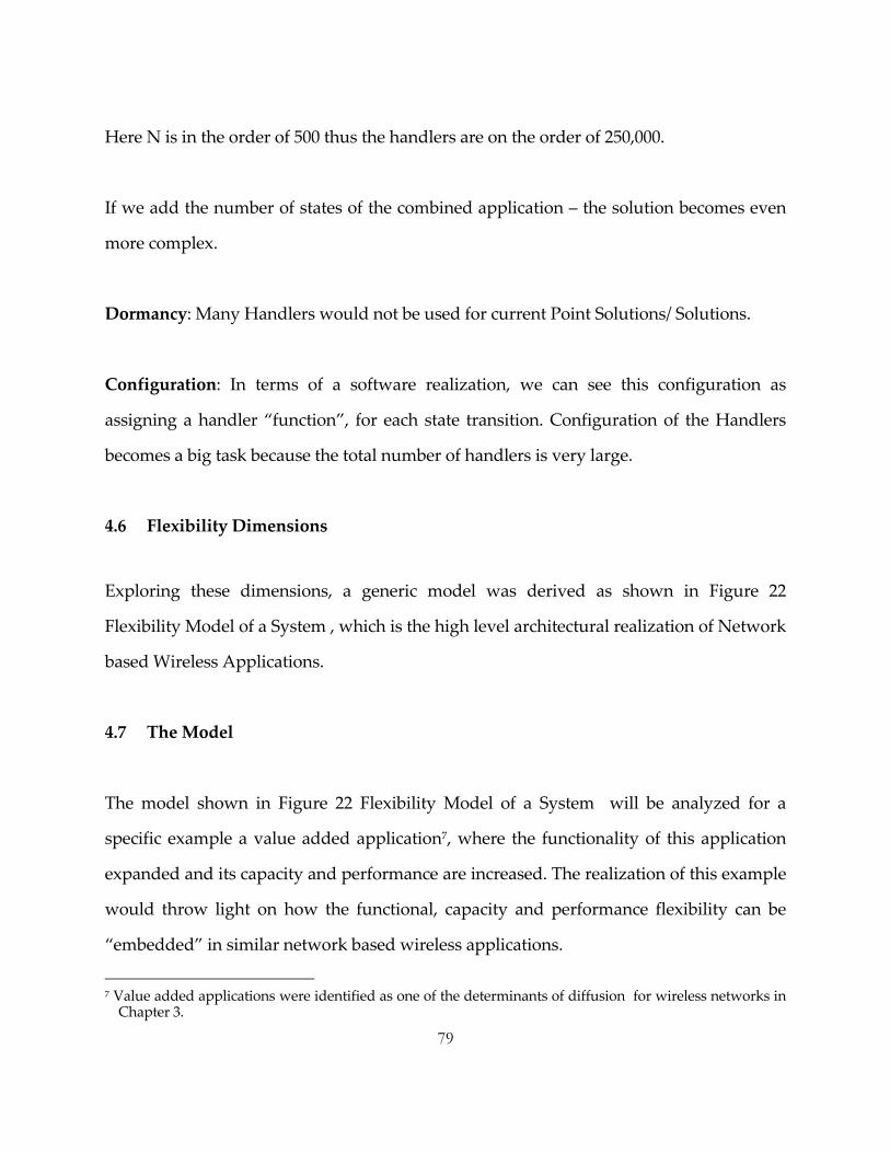
79
Here N is in the order of 500 thus the handlers are on the order of 250,000.
If we add the number of states of the combined application – the solution becomes even
more complex.
Dormancy: Many Handlers would not be used for current Point Solutions/ Solutions.
Configuration: In terms of a software realization, we can see this configuration as
assigning a handler “function”, for each state transition. Configuration of the Handlers
becomes a big task because the total number of handlers is very large.
4.6 Flexibility Dimensions
Exploring these dimensions, a generic model was derived as shown in Figure 22
Flexibility Model of a System , which is the high level architectural realization of Network
based Wireless Applications.
4.7 The Model
The model shown in Figure 22 Flexibility Model of a System will be analyzed for a
specific example a value added application7, where the functionality of this application
expanded and its capacity and performance are increased. The realization of this example
would throw light on how the functional, capacity and performance flexibility can be
“embedded” in similar network based wireless applications.
7 Value added applications were identified as one of the determinants of diffusion for wireless networks in Chapter 3.

80
Figure 22 Flexibility Model of a System
Our example application, Application 1, re‐connects dropped calls in a wireless network.
A high level intent‐ process‐concept diagram of the application based on Crawley’s OPM
framework [4] is shown in Figure 23 Intent‐Process‐Concept diagram of Application 1.
The intent of reducing the dropped calls is realized using the process of reconnecting
such calls, by monitoring the signaling information and restoring the context of the
dropped calls using Computer Telephony interfaces.
81
Figure 23 Intent‐Process‐Concept diagram of Application 1
The Attribute of transforming in the primary intent (which in this case is reducing
dropped calls) , the selected process (which in this case is re‐connecting dropped calls),
and the operating intent will drive the form related attributes (Attributes A and
Attributes B) as shown in Figure 24 Application Attributes.

82
Attribute Category Unit Connection Latency Performance sec Call Capacity Capacity Telephony Channels Cost Resource $ MTTF Performance years Maintenance cost Performance $/year Physical footprint Resource H x W x L and lbs Power consumption Resource KW
Figure 24 Application Attributes
The attributes compiled from the primary intent, process and operating intent for
Application 1, and their units are shown in Figure 24 Application Attributes. The
classification of the attributes in the three categories – Performance, capacity and
Resource, provide an practical insight of the theoretical context presented in Chapter 3,
Figure 5 OPD Representation of Flexibility: Capacity and Performance Flexibility.
It was interesting note that the attributes with a time component do conform to the
traditional definition of performance.

83
Figure 25 Architectural Form of Application 1
The connection latency, which is an obvious performance attribute, depends on the rate
of primary attribute transforming (i.e. how fast the dropped calls are reduced. The
Capacity attribute relates to the volume of the dropped calls. The architectural form of
Application 1, based on the model described in Figure 22 Flexibility Model of a System ,
is shown in Figure 25 Architectural Form of Application 1.
Application 1 can be implemented by monitoring the IS‐634 and ISUP Messages, which
have the call termination information. The External Interface monitors the signaling link
and extracts all the SS7 messages. The Protocol extracts the specific messages (Symbols)
that are required by the application from the SS7 signaling data, which in this case are
some specific IS‐634 and ISUP messages.

84
The Application layer SM, correlates these messages and for the cases the call was
abnormally dropped due to radio resource, initiates a two way call through the computer
telephony interface to the caller and called party and patches the call. This is done when
the wireless user re‐enters the network (comes out of a blind spot). This restores the
context of the call.
Functional Flexibility was defined as the ability of a system to perform additional tasks
under a changing set of requirements or operating conditions. In Application 1, we can
expand the functionality by sending an SMS with the dropped call details (called number
and time the call got dropped) to the subscriber, who can follow up on the call at his
convenience. This can be enabled by allowing dynamic addition of a new Application
State machines, or enabling some dormant states of an existing state machine. An
additional resource of SMSC connectivity is required for this added functionality as
shown in Figure 26 Architectural Form of Application 1 with Functional. These “slots”
have to be designed as part of the flexible system architecture and can be populated at a
later time to achieve functional flexibility. This is similar to the extensibility “master plan”
described in [9].
Capacity Flexibility could be defined as the capacity to address an additional (or a range of)
volume of interactions. This would be defined by total number of simultaneous
conversations taking place. In the example of Application 1, for example, if it takes 1Kb of
data to store the context of the call of one subscriber, the database size would be 1GB for 1
Million subscribers and 2GB for 2 Million subscribers. To increase the capacity of the
application from 1 Million subscribers, to 2 Million subscribers, the database has to be
scaled accordingly.

85
Figure 26 Architectural Form of Application 1 with Functional Flexibility
This can be achieved by using a scalable data storage network as shown in Figure 27
Architectural Form of Application 1 with Capacity Flexibility.
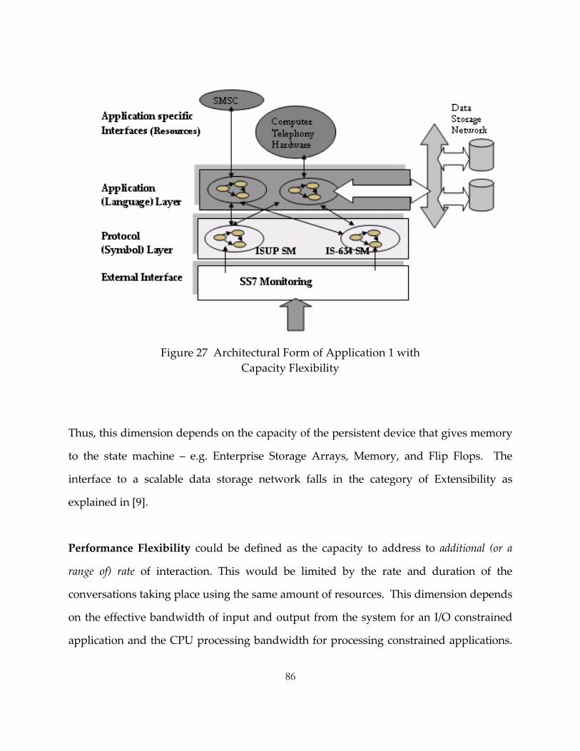
86
Figure 27 Architectural Form of Application 1 with Capacity Flexibility
Thus, this dimension depends on the capacity of the persistent device that gives memory
to the state machine – e.g. Enterprise Storage Arrays, Memory, and Flip Flops. The
interface to a scalable data storage network falls in the category of Extensibility as
explained in [9].
Performance Flexibility could be defined as the capacity to address to additional (or a
range of) rate of interaction. This would be limited by the rate and duration of the
conversations taking place using the same amount of resources. This dimension depends
on the effective bandwidth of input and output from the system for an I/O constrained
application and the CPU processing bandwidth for processing constrained applications.

87
In the example of Application 1, the connection latency, or the latency between the time
the call is dropped and it is re‐connected, was identified as a performance measure, based
on the primary intent and process attributes in Figure 24 Application Attributes.
This latency will drive a lot of design parameter, but at a high level, this latency will
depend on how “quickly” the application can acquire, retrieve, process and update the
state information of a transaction (or call). This means, we have to plan for scalability
across all these operations, to have performance scalability. Analyzing these operations in
detail we find that:
Acquire operations depend on the Input/Output bandwidth. This aspect of the
performance has to be resolved using a scalable I/O interface.
Retrieve and update operations depend on the database. For example it would take
higher average time to query a database of 2 Million users, than 1 Million users (using the
same indexing strategy). This aspect of the performance has to be resolved by using
scalable databases with flexible indexing / partitioning schemes.
Process operations depend on the processing bandwidth of the machine the application
is running on. This aspect of performance has to be resolved using a scalable application
architecture, with multiple instances of the same applications “load sharing” to
collectively scale the performance.
One method of implementing distributed applications is described in the Patent
application [32], which describes a way of distributing the Acquire, Process and Database

88
function to achieve a flexible solution, which is limited only by the back‐plane
bandwidth.
Figure 28 Distributed realization of Application 1
The application SM interface with the protocol SM through a distributed back‐plane via
distributed “adapters”. These adapters allow us to distribute the layers and functional
components of the Architectural form described in Figure 27 Architectural Form of
Application 1 with Capacity Flexibility in different computation units (Machines/ Servers)
as shown in
Figure 28 Distributed realization of Application 1.

89
Figure 29 The Three Dimensions Realized
Capacity/performance flexibility is achieved by scaling the database dimension and
adding more nodes to the network. The overall distributed architecture using the
distributed adapters is shown in Figure 29 The Three Dimensions Realized. The different
Application Servers enables functional flexibility. The different instances of one particular
Application Server enable part of performance flexibility (Process). The scalable database
interface enables the capacity flexibility and part of performance flexibility (retrieve
/update). The different instances of Peripheral server enables part of performance
flexibility (acquire).

90
Conclusion
It is shown by this analysis that the three dimensions of flexibility can be realized using a
distributed architecture (for wireless network applications). This distributed architecture
allows multiple applications, multiple instances of these applications and multiple
network inputs to interact. , enabling all the three dimensions of flexibility. Using the
example of Application 1, a network based wireless value added application; we found
that Application Servers executing different Application SM enable functional flexibility.
The different instances of one particular Application Server (Application SM) enable part
of performance flexibility (Process). The scalable database interface enables the capacity
flexibility and part of performance flexibility (retrieve /update). The different instances of
Peripheral server enables part of performance flexibility (acquire). The example of the
value added application was chosen to investigate the aspect of embedding flexibility as
it illustrates all the three dimensions of flexibility. In the next chapter we will build the
framework which would be used to identify and formally access the cost and value of
implementing a flexibility design space (see Figure 8 Flexibility Design and Objective
Space. Adapted from [6].), after the flexible objective space has been defined (as shown in
Chapter 3) and its implementation feasibility verified (as shown in Chapter 4).

91
C h a p t e r 5
Valuing Product Flexibility (Mathematical Framework)
5.1 Introduction
In this chapter we explore the methods that can be used to model the payoffs associated
with the flexible design options with respect to the costs incurred to implement design
flexibility options in the face of uncertainty. In the subsequent sections, a framework is
developed for assessing the cost and value of these design options.
The example cited in Chapter 3 describes the scenario where the on‐chip cache size plays
an important role in overall performance of the wireless handset from the context of
different potential applications. Similarly, implementing a processor design optimized for
only single threaded applications or multi‐threaded applications leads to the constraint of
meeting needs of only one market segment. There is uncertainty associated with how the
application scenario, and with it the demand for higher single threaded performance or
multi‐threaded applications, will evolve.
The example of distributed network application explained in Chapter 4 (Embedding
Flexibility), involves design and implementation of distributed adapters, which can
enable scaling in terms of Functionality, Capacity and Performance. Similar to the
example of wireless handset processors , by implementing these flexible design features
we can potentially maximize the net benefit by meeting new market needs which may

92
translate into a higher revenues when the Network application can scale for increased
Functionality , Capacity and Performance requirements
This analysis illustrates the different ways of calculating the value of a flexible design
option using the example of a hypothetical example of a Wireless Handset processor
manufacturer.
5.2 Flexible Wireless Processor.
A processor design optimized for only a particular class of application, leads to the
constraint of meeting needs of only one market segment. There is an uncertainty
associated with how the application scenario, will evolve. Implementing design features
for a flexible feature (e.g. cache architecture), we incur a cost in terms of additional design
effort, complexity and allocation of resources, which detract from traditional performance
metrics (for example it may lead to higher power and die cost ).
By implementing flexible design features which enable optimization of applications, by
enabling of an additional on‐chip cache at a later decision point in time we can potentially
maximize the net benefit by meeting new market needs which may translate into a higher
ASP (average selling price) for each unit when the new features are enabled.
5.2.1 Background

93
PixelAirDSP is a “fab‐less”8 DSP Company, and makes high performance Digital Signal
Processors (DSP) for the wireless Handset segment.
It had a design win with Smartest, a major handset manufacturing company in Japan,
which makes “smart” wireless handsets, customized for a large GSM based Mobile
Network Operator (MNO) CarryAll, in Europe.
Currently the handsets that are being manufactured are for voice applications only.
CarryAll wants to offer the 2.5G GPRS data services next year.
PixelAirDSP has been asked by Smartest to provide a DSP solution, which would provide
a differentiated performance for digital video applications that would be based on GPRS
Data services. The performance criterion is the total clock cycles expended by a low
bandwidth codec (H.264), for a reference digital video sequence, for a standard resolution
and frame rate.
Predicted handset diffusion data for next three years have been provided for different
conditions.
PixelDataDSP’s design simulations show that modification of two critical blocks would
make their (under early design) 2.5 G DSP, perform satisfactorily for 3G bandwidths. One
of the blocks is the on‐chip cache architecture. Let us assume PixelDataDSP has two
choices –
8 They outsource fabrication to a company in Taiwan.

94
Option 1 ‐ Design a 2.5 G DSP for the handsets that would be required next year and
Design 3G DSP, when there is a certainty of the 3G rollout. This will involve another
development cycle , where most of the design would be shared but due to substantial
“backend flow” costs , which are the costs of validating the processor design once it is put
in silicon , it is estimated that the second development cycle would cost 50% of the first
cycle cost of $20 Million.
Option2 – Design a “flexible’ cache architecture, which would cater to both 2.5G and 3G
bandwidths. This would cause an additional design cost of $5 Million to the original
design cost. The 3G cache features can be “enabled” at a later point of time, with an
additional cost of $ 1 Million (primarily, a new production setup cost).
Assumptions:
1. There could be a reduction of the overall yield due to increased die size. This is the
penalty in terms of the variable costs incurred due to the “additional” slots of a
flexible design. For simplicity of the analysis, this is assumed negligible in our
analysis.
2. It is assumed that the total design/production effort of PixelDataDSP is locked in
to Smartest (and vice versa). This assumes there is no cost due to potential loss of
market opportunity i.e. Smartest would not use an already available 3G DSP
solution from a PixelDataDSP’s potential competitor.
3. The Average selling price for both the 2.5G, 3G and Hybrid DSP is $30.

95
We will explore in the following section, using this example, the different ways
PixelDataDSP can assess the flexible option.
5.2.2 Value of the flexibility option
This analysis is based on the Dual‐Fuel Burner example [Error! Reference source not
found.]. We start the analysis with an analogous assumption that the demand data is
known with certainty and then introduce uncertainty to this data.
Certain Demand – Development Cost scenario.
In this scenario, CarryAll plans a 3G network rollout in year two and predicts a “certain”
market diffusion data as shown in Figure 30 Market diffusion prediction. This data is
considered to be “certain” demand at this point of time as most of the new handsets
would replace the existing handset (which is a known data) and the market growth per
year has been consistent for last five years.
This would necessitate introduction of new 3G handsets in the Year 2, supporting high
bandwidth (2 Mbps) codec’s like MPEG4.
Cash Flows under certain demand
The cash flows under certain demand are shown in Figure 31 Cash Flows under certain
demand .

96
0
2000
4000
6000
8000
10000
Year1 Year2 Year3 Year4 Year5
Year
Num
ber o
f Han
dset
s ('0
00)
2.5G DSP 13G DSP 1
Probability Year1 Year2 Year3 Year4 Year5
2.5G DSP 1 1000 2000 3000 4000 2000
3G DSP 1 0 500 1000 4000 8000
Figure 30 Market diffusion prediction
The Expected Cost of enabling the flexibility feature, as seen in the cash flow, is incurred
in the year 3, when there is actual demand for the product (there is an underlying
assumption that the feature can be activated with no delay). In the fixed case option, the
cost of designing the 3G processor is incurred a year before the actual demand (which
would be typical).

97
CASH FLOWS ('000 $) CERTAINITY
Discount rate 5%
Year 1 2 3 4 5 Option1 Revenue 30000 75000 120000 240000 300000
(Fixed) Cost 20000 10000 0 0 0
R-C 10000 65000 120000 240000 300000
Present Value 9523.81 58956.92 103660.5 197448.594 235057.8
NPV 604647.7
Option2 Revenue 30000 75000 120000 240000 300000
(Flexible) Cost 25000 0 1000 0 0
R-C 5000 75000 119000 240000 300000
Present Value 4761.905 68027.21 102796.7 197448.594 235057.8
NPV 608092.2
Figure 31 Cash Flows under certain demand
Recommendation
Based on this analysis, (for this particular example) the flexible option is better than the
fixed option even in the condition of certain demand. It has been widely published in the
literature that flexibility is only valuable under uncertain conditions . This view, however,
does not incorporate the engineering cost analysis and is based largely on uncertainty
analysis of the benefits.
The hypothesis here is that flexible implementation can be a better option as compared to
the fixed implementation due to differential development costs, even under the
conditions of certainty. The flexibility option has a value in case of certainty when the

98
cumulative fixed development costs exceed the cost of flexible implementation and
activation of the flexible feature. This hypothesis is based on the simplifying assumptions
that there are no variable cost penalty for the flexible implementation and that the
diffusion curve is same for fixed and flexible solutions.
Uncertain Demand – Flexible Activation Scenario
There is a uncertainty in CarryAll’s plans of 3G network rollout in the year two. This
decision will be based on the observation of market response for 3G services for
MobiKom and 3 (The two 3G based MNO’s in Europe). This would necessitate
introduction of new 3G handsets, supporting high bandwidth (2 Mbps) codec’s like
MPEG4.
The predicted units of units sold with their probabilities are shown in Figure 32
Predicted 3G units sold with uncertainty (delayed 3G rollout). We have retained the
original 2.5 G , to facilitate easy comparison.
Probability Year1 Year2 Year3 Year4 Year5
2.5G DSP 1 1000 2000 3000 4000 2000
3G DSP 0.5 0 500 1000 4000 8000
0.4 0 0 500 1000 4000
0.1 0 0 0 500 1000
Figure 32 Predicted 3G units sold with uncertainty (delayed 3G rollout)

99
This scenario illustrates a condition where there is a possibility of a delayed rollout due to
unfavorable consumer response. The cash flows for the two options under this condition
are shown in Figure 33 Cash Flow under uncertain demand. The Expected value of
Revenue, Cost, Present Value and Net Present value are calculated based on the
probabilities shown in Figure 32 Predicted 3G units sold with uncertainty (delayed 3G
rollout). The Expected Cost of enabling the flexibility feature, as seen in the cash flow, is
distributed in the years 3, 4 and 5 (immediate activation assumption). The cost for a fixed
3G design is similarly distributed across three years 2, 3 and 4 (design latency
assumption).
CASH FLOWS ('000 $) UNCERTAINITY
Year 1 2 3 4 5 Option1 E(Revenue) 30000 67500 111000 193500 231000
(Fixed) E(Cost) 20000 5000 4000 1000 0
E(R-C) 10000 62500 107000 192500 231000
E(Present Value) 9523.81 56689.34 92430.62 158370.226 180994.5
E(NPV) 498008.5
Option2 E(Revenue) 30000 67500 111000 193500 231000
(Flexible) E(Cost) 25000 0 500 400 100
E(R-C) 5000 67500 110500 193100 230900
E(Present Value) 4761.905 61224.49 95454.05 158863.848 180916.2
E(NPV) 501220.5
Figure 33 Cash Flow under uncertain demand

100
5.2.3 Recommendation
The flexible option is better than the fixed option, even in the condition of uncertain
demand. The simplifying assumptions that there are no variable cost penalty for the
flexible implementation and that the diffusion curve is same for fixed and flexible
solutions, that were made in the analysis of certain demand, applies for this case too.
Analysis
A comparative analysis of the relative advantage of the flexible product is shown in
shown in Figure 34 Relative advantage of Flexible DSP.
Certainty Uncertainty
% NPV gain 0.569679 0.644957
with Flexibility
Figure 34 Relative advantage of Flexible DSP
This can be substantiated by the fact that (all other things remaining constant) the cost of
enabling the flexibility feature can be delayed based on the market scenario. This delayed
cost increases the estimated NPV. Higher the activation cost, greater will the relative
benefit under uncertainty as shown in Figure 35 NPV Gain with increased Activation
Cost.
In this simplified analysis we assumed that the cost of designing a flexible product and
activating the features is less than two cycles of fixed designs. We also assumed that the
fixed designs and flexible design command the same price premium and incur the same
costs.

101
Costs (Million$)
Fixed Design Cost Flexible Design Cost
%NPV Gain
2.5G 3G
2.5/3G
Design Activation
20 10 25 1 0.64495743
21 5 0.73574185
16 10 0.84922238
11 15 0.96270291
6 20 1.07618344
1 25 1.18966396
Figure 35 NPV Gain with increased Activation
Cost.
In cases where the cost of the flexible design exceeds the cumulative cycle cost of fixed
design, the differential cost has to be compensated by a price premium of the flexible
product else Flexibility strategy should not be recommended.
In the cases where the Flexible design costs are “Front Loaded”(little or no activation
costs) in addition to the overall cost disadvantage, this recommendation is especially
important.
5.3 Quantitative Framework
In this section we build a quantitative framework to extend our initial analysis of one
flexibility attribute – Processor performance for digital video codec, to multiple attributes.

102
5.3.1 Flexibility Attributes
Each one of the three dimensions of flexibility: Functionality, Performance, and Capacity,
consists of many attributes, which can also be thought of as requirements. These
requirements would define the form related design attributes and map into a part of the
overall objective space, by defining the flexible objective space as shown in Figure 8
Flexibility Design and Objective Space. Adapted from [6]. However, we reserve the word
“requirements” for concrete mandatory needs required for the delivery of the system,
while these attributes are based on a prediction of what the system might morph into in
the future. The attributes of the three dimensions are therefore:
Functional attributes:
Fa = [Fa1, Fa2, …, Fal] (1)
Where l is the number of Functional attributes.
Performance attributes:
Pa = [Pa1, Pa2, …, Pam] (2)
Where m is the number of Performance attributes.
Capacity attributes:
Ca = [Ca1, Ca2, …, Can] (3)
Where n is the number of Capacity attributes.

103
In the example of wireless handset processors discussed in the previous section, the
“Performance attribute” is the total clock cycles expended by a low bandwidth codec
(H.264), for a reference digital video sequence, for a standard resolution and frame rate.
5.3.2 Time Window
These attributes may have different time windows associated with them, in our example,
performance scaling in the wireless handset processors for digital streaming video
applications, imposes a Performance attribute to handle 56Kbps – 2 Mbps data streams
within a period of five years. Similarly, capacity scaling in the case of a wireless network
application may have requirement to scale from 1 Million to 2 Million subscribers in a
period of five years.
The time windows corresponding to the functionality attributes are therefore:
Functionality Time Window:
Tf = [Tfa1, Tfa2, …, Tfal] (4)
Where l is the number of Functional attributes.
Performance Time Window:
Tp = [Tpa1, Tpa2, …, Tpam] (5)
Where m is the number of Performance attributes.
Capacity Time Window:
Tc = [Tca1, Tca2, …,Tcan] (6)
Where n is the number of Capacity attributes.
104
The functionality attributes that are mapped to design parameters have an overall time
window Tw, which is the maximum of all individual time windows.
Tw = Max (Max (Tfa1, Tfa2, …, Tfal),
Max (Tpa1, Tpa2, …, Tpam),
Max (Tca1, Tca2, …,Tcan )) (7)
5.3.3 Flexibility Design Space
Through various existing systems engineering methods, like QFD [1673] these
functionality attributes (similar to requirements) can be related to design parameters.
These parameters constitute the flexibility design trade space.
The flexibility design parameters vector is therefore:
Dp =[Dp1, Dp2, …, Dpk] ( 8)
Where k is the number of design parameters that map to the flexible design space. It
contains all the flexibility design parameters. In the example of the wireless handset
processor, if the performance flexibility is realized using a 2X on‐chip cache AND an
enhanced Direct Memory Access (DMA),
Dp =[Dp1, Dp2 ] (9)
105
Where,
Dp1 ‐ 2X on‐chip cache.
Dp2 ‐ Enhanced DMA.
5.3.4 Current Costs
The Dp vector is associated with current implementation cost. This cost is
comprehensive, and should include the costs resulting form various aspects of the
implementation:
• Cost of design
• Cost of manufacturing
• Cost associated with product delays to accommodate for the flexibility design
• Cost associated with the incremental risk added to the system as a whole as a
result of the flexibility design
The result is a flexibility cost vector:
Cf =[Cf1, Cf2, …, Cfk] ( 10)
Where k is the number of design parameters.
5.3.5 Future Costs
There is a cost vector (in the future) for implementing the flexibility option, in other
words activating the built‐in flexibility features. Note that this is different from the cost
of designing flexibility which was described in the previous section. This cost is

106
dependent on the design decisions made at t0, i.e. on the flexibility design parameter
vector Dp.
Ci(Dp) =[Ci1, Ci2, …, Cik] (11)
Where k is the number of design parameters.
5.3.6 Value
Along with the cost, there is a value associated with implementing the flexibility. This
value can be represented by the vector Vi. This value is dependent on the state of the
future F(t).
Vi(F(t), Dp) = [Vi1, Vi2, …, Vik] (12)
Where k is the number of design parameters.
In the example of wireless handset processor, we estimated this value under certain and
uncertain future and found that the value of flexible options increases with increasing
uncertainty.
5.4 Real Option Approach
The traditional method that companies use to select which projects or designs to invest in,
Discounted Cash Flow analysis (DCF) or Net Present Value (NPV) calculations, does not
always accurately represent the actual value of the projects under study [14]. That is
because DCF assumes that we will follow a predetermined path.

107
In reality, uncertainty and investment choices exist together and these choices are spread
over time. As uncertainty changes, downside losses can be avoided by not investing more
funds into projects which have poor performance [15]. In our case, this investment relates
to the cost of embedding flexibility in the product.
We use the concept of real options to calculate the call value of the option, based on the
earlier work of Black and Scholes. In our case this is the value of embedding flexibility in
a product design.
This section provides a mechanism to compute the value of the flexibility option Vf (Eq.
12), that is, the value of embedding multi‐attribute flexibility in the design. There are
multiple methods to compute Vf using Real Option Analysis. Amram and Kalutilaka[17]
propose three high level solutions:
• The PDE approach, by solving a partial differential equation to obtain the value of
the option from a tracking portfolio.
• A dynamic programming approach that lays out the future and folds back the
optimal strategy.
• A simulation approach that picks the optimal value strategy by simulating all
possible outcomes.
We will look at two of these solutions and map them to our problem.
5.4.1 Black‐Scholes Model (PDE)

108
The Black‐Scholes model is simple to implement once all the variables have been
identified. It consists of an equation that computes the value of the option given the
following variables:
Cost of exercising the option,
Current value of the underlying asset,
Risk free interest rate,
Time to expiration, and
Volatility of the underlying asset
Other than ensuring a proper mapping, one needs to verify the boundary conditions of
the formula. The Black‐Scholes formula [1676] for the valuation of financial stocks is the
following:
V = N(d1) A – N(d2) X e‐rT (13)
Where
V = Value of call option
A = Current value of underlying asset
X = Exercise price
T = Time of expiration
r = Risk free interest rate
σ = Volatility of underlying asset
N(d) = Cumulative value of normal distribution at d

109
d1 = ln (σ/X) + (r + 0.5 σ2 )T )/(σ.Sqrt (T)) (14)
d2 = d1 ‐ σ.Sqrt (T) (15)
This formula models European call options. European options can only be exercised at
the expiration time T. On the other hand, American options can be exercised at any time
between t0 and T. In modeling flexibility using real options, although the most accurate
model is the American one, we can justifiably use the European model by assuming that
at the time of the valuation of the flexibility (design phase), one can predict to a degree of
certainty the time at which this flexibility would be activated . This time is Tw as shown
in Eq.8.Moving forward with the European model, we can then map the flexibility real
options parameters to the financial parameters as shown in Figure 36 Mapping Design
Flexibility Options to Financial Options.
FINANCIAL
CALL
OPTION
PARAMETERS
FLEXIBILITY OPTION
PARAMETERS
COMMENTS
Option value V Value of designing
flexibility
Vf
Option price P Cost of designing
flexibility at time 0
Cf
Exercise price X Cost at time T of
implementing the
flexibility
Ci

110
Current stock
price (price of
underlying
asset)
A Current value of
implementing flexibility
Vi The mapping of this
variable still needs some
careful manipulation to
ensure that it matches the
boundary conditions of
the Black‐Scholes model
Time to
expiration
T Time at which the
flexibility would be
implemented
Tw To fit the Black‐Scholes
model, there is an
assumption that the time
between incurring cost Ci
and getting value Vi is
zero. In reality, this time
is not zero and the
equation would have to
be adjusted to account for
it by time shifting either
Ci or Vi.
Risk free
interest rate
r Risk free interest rate R
Volatility of the
stock price
σ Volatility of the expected
benefit of implementing
the flexibility
σ This is estimated in
Chapter 7.
Figure 36 Mapping Design Flexibility Options to
Financial Options
111
In order to successfully utilize this model, we need to identify a method for computing
the risk free interest rate as well as the volatility of the expected benefit of implementing
flexibility. Moreover, we need to be able to determine and quantify Vi. A proposal for
how to accomplish that is presented in the Chapter 6 [Assessing Flexibility: Option
Parameters and Cost].
Limitations of Black‐Scholes
The Black‐Scholes formula assumes the existence of a replicating portfolio and no
arbitrage [33]. The absence of data on replicating portfolio for flexible options makes the
estimation of the value of the underlying asset less accurate. Since flexible product
options in innovative industries are not traded on open security markets it is difficult –
and often impossible – to find a replicating portfolio for assessing the value of a
particular, flexible product feature as a European or American Call Option. The value of
the underlying asset can be subjectively estimated [16], but the results of the Black‐
Scholes formula would not be accurate [39]. The formula, however, can be used for
qualitative comparison between different flexibility options and in cases where a similar
flexible product is already in the market and the value of the flexibility (and volatility) is
known.
Black Scholes Valuation of Flexible Processor Architecture
The following example illustrates the application of Black Scholes option model to
calculate the economic value of flexible system design for handset processor architecture.
The traditional CPU architecture can be enhanced during the concept engineering phase
to incorporate flexible features which have a potential market and economic value. The
flexible design variants which are enabled in this case are:

112
Option Flexible design variantA integrates multi-threaded architectureB integrates high performane graphics coreC integrates encryption hardwareD integrates memory controllerE integrates ultra low power mode to conserve battery lifeF integrates support for 64 bit applications
Figure 37 Flexible Design Variants for a Processor
As discussed earlier we can determine through Conjoint Analysis which features present
the greatest utility to the end customer, what combination of features constitute a viable
design variant and also the price differential represented by higher ASP we can expect by
enabling some of the latent features in a given CPU architecture at a later point in time.
We can estimate the potential market by looking at the future growth trends for some of
the features in a stand alone component and by estimating the projected diffusion curve
of capturing a certain market segment share of integrating some of these features into an
existing CPU architecture. Specifically, we can easily get market research data for the
discrete graphics market share for high end graphics card in the future. By using
appropriate diffusion curves we can make predictions for the adoption of an integrated
design as a function of time. The cost of enabling a flexible design feature can be
estimated on a case by case basis. For example, integrating a high end graphics engine
would result in die size increase, yield impact, higher power consumption leading to
higher cooling costs and additional design and validation costs. All these can be
ascertained and quantified. The delay in time to market due to higher complexity can also
be translated into lost revenue which is factored into enabling any one of the design
variants.

113
In applying the Black‐Scholes model, the hardest parameter to estimate accurately is the
variance associated with future returns of a flexible design variant. To determine this we
can identify the returns with the new product to the variance of a similar feature in the
past. One consideration if we use this approach is to look at the variance at least as far
back in time as the period in the future for which we are calculating the real option value.
Figure 38 Diffusion Curve
As illustrated in Figure 39 Black Scholes Valuation of Flexible CPU Architectures, the
design variant which integrates a high performance graphics core has a NPV of $25
million but the real option value is $48.14 million. This is due to the large time to
expiration of 5 years and standard deviation of 30%. Similarly design variant which
integrates support for 64 bit application has NPV of ‐$25 million but the option value of
$10.15 million due to 3 years to expiration and a standard deviation of returns of 40%.
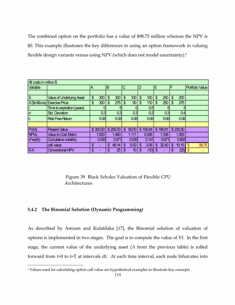
114
The combined option on the portfolio has a value of $98.75 million whereas the NPV is
$0. This example illustrates the key differences in using an option framework in valuing
flexible design variants versus using NPV (which does not model uncertainty).9
Variable A B C D E F Portfolio Value
S Value of Underlying Asset 300$ 300$ 100$ 100$ 250$ 250$ X ($millions) Exercise Price 300$ 275$ 90$ 110$ 250$ 275$ t Time to expiration (years) 0 5 0 0.5 5 3σ Std. Deviation 0.3 0.3 0.3 0.2 0.3 0.4rf Risk Free Return 0.06 0.06 0.06 0.06 0.06 0.06
PV(X) Present Value 300.00$ 205.50$ 90.00$ 106.84$ 186.81$ 230.90$ NPVq Value to Cost Metric 1.000 1.460 1.111 0.936 1.338 1.083 σ*sqrt(t) Cumulative volatility 0.000 0.671 0.000 0.141 0.671 0.693
call value -$ 48.14$ 5.00$ 3.06$ 32.40$ 10.15$ 98.75$ -$ S-X Conventional NPV -$ 25$ 10$ (10)$ -$ (25)$
All costs in million $
Figure 39 Black Scholes Valuation of Flexible CPU Architectures
5.4.2 The Binomial Solution (Dynamic Programming)
As described by Amram and Kulatilaka [17], the Binomial solution of valuation of
options is implemented in two stages. The goal is to compute the value of Vf. In the first
stage, the current value of the underlying asset (A from the previous table) is rolled
forward from t=0 to t=T at intervals dt. At each time interval, each node bifurcates into
9 Values used for calculating option call value are hypothetical examples to illustrate key concepts
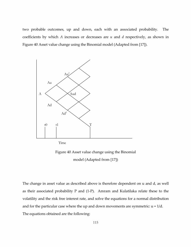
115
two probable outcomes, up and down, each with an associated probability. The
coefficients by which A increases or decreases are u and d respectively, as shown in
Figure 40 Asset value change using the Binomial model (Adapted from [17]).
Figure 40 Asset value change using the Binomial
model (Adapted from [17])
The change in asset value as described above is therefore dependent on u and d, as well
as their associated probability P and (1‐P). Amram and Kulatilaka relate these to the
volatility and the risk free interest rate, and solve the equations for a normal distribution
and for the particular case where the up and down movements are symmetric: u = 1/d.
The equations obtained are the following:
Au2
Au
A Aud
Ad
Ad2
t1
Time
t0 T

116
u = er (16)
d = 1/u (17)
P = (er ‐d)/(u‐d) (18)
Where:
r is the risk free interest rate.
In the second stage, the values obtained at the end nodes of the resulting tree are folded
back. The option to exercise is reflected using the following rule at the end nodes
ATn = max[ATn‐X, 0] (19)
Where:
ATn is the value of the asset at time T and end node n
X is the cost to exercise the option
The values are folded back according to the equations shown in Figure 41 Binomial
method (stage 2). Rolling back to obtain the value of flexibility.

117
Figure 41 Binomial method (stage 2). Rolling back
to obtain the value of flexibility
Rolling all the way back to time t0 yields Vf, the value of embedding the flexibility in the
design. Similarly to what was mentioned in the Black‐Scholes model, this computation is
dependant on the value of the underlying asset (A or Vi) as well as the volatility and time
to expiration. Unlike Black Scholes , however , it does not assume the existence of a
replicating portfolio and thus the quantitative results using Binomial method would be
more accurate than Black Scholes in cases where the assumption of existence of a
replicating portfolio does not hold.
AT1
= ((P.AT1) + ((1-P).AT2)).e‐r
AT2
Vf
ATn
Time

118
5.5 Conclusion
The value of embedding flexibility can be assessed using the real options approach. The
Black‐Scholes model and the Binomial model can be used to compute the value of flexible
design options. The decision of implementing the flexibility is analogous to the financial
decision of exercising the option, and the cost of implementing the flexibility is analogous
to the exercise price of the option.
We found in the case study of a flexible mobile handset processor that the value of
flexibility does increase with increasing uncertainty. We also found that by moving the
cost of embedding flexibility to the later or “activation” stage, the value of the flexible
option increases as compared to a “front loaded” flexibility cost.
We established a mathematical framework for a multi‐attribute flexible product and
mapped these attributes to flexible design options. The parameters used in option
calculations ‐ value of the underlying asset, time to expiration and cost of embedding
flexibility, have been defined under a mathematical framework in this chapter. The next
chapter would describe some of the methods that can be used to compute these
parameters.
119
C h a p t e r 6
Assessing Flexibility – Option Parameters and Cost
6.1 Introduction
We have modeled the present situation vis‐à‐vis flexibility, its dimensions, its attributes,
the design parameters to implement these attributes, as well as the costs associated with
these design parameters. We now take a look at the future market potential of a flexible
product. This analysis is to determine the value of the underlying asset, and the volatility
of this value. This, by far, are the most difficult parameters to access in the flexibility
analysis.
Our intention is to calculate the mean value of the underlying assets (Eq. 12) and it’s
volatility over the time to expiration. At a given point of time, the mean value can be seen
as the product of the number of units of the product and the incremental price a customer
is willing to pay for the flexible features. Since both these distributions can be assumed to
be normally distributed, the effective distribution will be a convolution of these two
normal distributions.
Let P be the normal distribution of the price a customer is willing to pay for a flexible
feature (we describe two methods to do this in later sections),at a given time where:
P = N (µp ,σp2) (20)
Where µp ,σp2are the mean and variance of the distribution.

120
Let U be the normal distribution of the units expected to be sold in the same time the
Price was determined10 (we describe two methods to do this in later sections), where:
U = N (µu ,σu2) (21)
Where µu ,σu2 are the mean and variance of the distribution.
The resultant distribution of Value, V , which is the product of these two distributions at
a given time , will have the mean µu ,
µu = µu * µp (22)
The resultant distribution will not be normally distributed [41] . If we use this mean value
of “Value” and plot this over time, we can calculate the Mean of this distribution over
time (mean value of the underlying asset) and the volatility (variance over time) , as
shown in Figure 42 Components of the Value distribution over time.
10 In this example we assume that “Price’ and “Number of units sold” are independent random variables , for illustrative simplicity.

121
µv
Figure 42 Components of the Valuover time.
6.2 Future Demand
The future can be modeled by a Future demand vec
elements: needs element, technology element, str
competitor element, and economy element. For exam
customer needs at any point in time in the future
represent technology availability at any point in time
written as a function of time:
F(t) =[Nf, Tf, Sf, Mf, Cf, Ef]
(N=need, T=technology, S=strategy, M=market, C=competito
µvT = µnT * µpT
Predicted Units Sold
µpT
Predict mium for flexible features
TimeValue
ed Price pre µnT
e distribution
tor, comprised of several types of
ategy element, market element,
ple, the needs elements represent
. Similarly, technology elements
in the future. This vector can be
(23)
rs, E=economy)
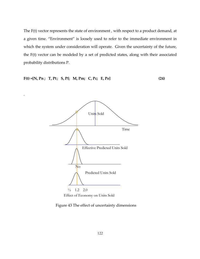
122
The F(t) vector represents the state of environment , with respect to a product demand, at
a given time. “Environment” is loosely used to refer to the immediate environment in
which the system under consideration will operate. Given the uncertainty of the future,
the F(t) vector can be modeled by a set of predicted states, along with their associated
probability distributions P.
F(t) =[N, Pn ; T, Pt ; S, Pf; M, Pm; C, Pc; E, Pe] (24)
.
Figure 43 The effect of uncertainty dimensions
No Predicted Units Sold
Effective Predicted Units Sold
Units Sold
Time
½ 1.2 2.0 Effect of Economy on Units Sold

123
This vector represents the cone of uncertainty. There would ideally be probability
distributions (discrete or continuous) for the effect of a particular component on the
normalized demand of a product.
This is shown in Figure 43 The effect of uncertainty dimensions , where the convolution
of the effect of the economy on the demand distribution and the predicted unit sold
distribution at a given time, gives the effective predicted units sold distribution, mean
value of which is represented in the overall product diffusion curve over time. The
effective distribution will not be normally distributed (as shown in the figure, for
simplicity) but the mean of this distribution will be the product of the means of the two
distributions [41]. The effect of all the other factors described in Eq. 20, can also be
factored in a similar way.
6.2.1 System Dynamics Model
Systems dynamics model has been successfully used to predict the future market and can
be used in conjunction with the other tools to predict the future penetration of a product.

124
Figure 44 Causal Diagram of 3G Capacity 11
One of the determinants of diffusion for wireless networks identified in Ch
the network capacity. 3G Networks provide a higher capacity than tra
networks, an illustrative causal diagram of the manufacture and deploy
networks, with a higher capacity, is shown in Figure 44 Causal Diagram of 3G
When the carrying capacity of the system based on demand saturates, the or
3G rollout declines. Due to time delays in the system, overcapacity result
followed by rapid decline in new orders leading to even more unutilized cap
characteristics of the system lead to the expected slow rollout and underutili
3G Networks.
11 This diagram is based on the Fiber Capacity boom‐bust causal diagram illustrated in Dynamics for Business Policy)
Raw FinishedWIP Installedgoodsinventorymaterials inventory base f fiberTelecom demand
Capacity on order
CapacityunderconstructionProductioncapacity
Production starts Productioncompletion rate
Raw materials acquisitions
oConstruction startsCapacity
acquisition
+
-
Installation orders
+
Bandwidth
3G
+
+
B
o
apter 3 was
ditional 2 G
ment of 3G
Capacity .
ders for new
s which are
acity. These
zation of the
15.874 (System
Obsolescence rate
rders

125
6.3 Value to Customers
In order to determine the estimated market potential of different flexible design features
which are embedded in a product platform, extensive market research is required with
lead users. Value Benchmarking [21] is used to determine how the product attributes
contribute to the value differences. Conjoint analysis is used to value the utility of the
product features. Contingency analysis is used to comprehend the value of social and
environmental factors on value. Direct value methods use a combination of both conjoint
and contingency analysis for assessing feature value to customers.
In the subsequent section, we review the applicability of Conjoint analysis and Kano
analysis methods, in determining which product features to enable and also to ascertain
the incremental cost customers are willing to pay for a product with the flexibility
features enabled. A critical factor to consider in this regard is the correlation between
stated preference and actual action in terms of purchase.
6.3.1 Conjoint Analysis
Conjoint analysis is a quantitative method used to identify and prioritize the preferences
of multiple product features. A convenient aspect of this method is that the price a
customer is willing to pay for a product feature can be embedded as one more variable in
the analysis. This method uses a customers ranking of a combination of global product
attributes and then decomposes it into a scale of utility attribute for each attribute or a
group of attributes. It uses orthogonal arrays in the design of the market survey

126
responses to minimize the explosion in the number of potential product variants
presented to the customer [22].
We have used the example of flexible handset processor that was described in Chapter 5
to illustrate this method. Consider a flexible design which has an option to optimize
either single threaded performance or multi‐threaded performance but not both. Higher
performance along either one of these attributes results in increased die size and higher
power (reduced battery life). It also translates into higher system costs. If we want to find
the preferences of the consumers to enable any one of the design options we can rely on
conjoint analysis.
If the single threaded performance has three levels (ST‐, ST0, ST+) where ST0 corresponds
to baseline performance, Multi‐threaded performance has similar three levels (MT‐, MT0,
MT+). The ‐/+ suffix indicate lower or higher performance from baseline. Let’s assume we
impact the battery life by two levels (BAT‐, BAT+). Expected increase in CPU ASP
(average selling price) due to improved performance is categorized as (Pr‐, Pr+, Pr++)
where Pr+ is higher performance and Pr++ the highest performance. The mobility vector
is again specified by two levels corresponding to increased thermal requirements for
higher performance leading to additional thermal system volume denoted by (Mob‐,
Mob0).
The complete combination of all product attribute, (each level is correlated to a product
architecture choice), results in 3x3x3x2x2 = 108 combination. Using Orthogonal arrays as
described in [21] we can reduce the possible design variations presented to the consumers
to 18.

127
Figure 45 Orthogonal Array for Processor Design
using Conjoint Analysis
The ranking of the customer preferences from the survey group for each design variant is
used to translate into a utility scale [0<=utility<=1] for each product attribute and for each
level of the attribute. The boundary condition for the utility is that the summation of the
utility for each design variant (as a function of the sum of the utilities of the individual
attribute level) matches the ranking average of the particular design variant based on the
survey response.
Using the conjoint analysis data, we can extract the following information:
Design Variant
Multi_Threaded Performance
Single-Threaded Performance Price
Battery Life Mobility
1 MT- ST- Pr0 Bat- Mob-2 MT- ST0 Pr+ Bat- Mob03 MT- ST+ Pr++ Bat+ Mob-4 MT0 ST- Pr+ Bat+ Mob05 MT0 ST0 Pr++ Bat- Mob-6 MT0 ST+ Pr0 Bat- Mob-7 MT+ ST- Pr++ Bat- Mob08 MT+ ST0 Pr0 Bat+ Mob-9 MT+ ST+ Pr+ Bat- Mob-
10 MT- ST- Pr++ Bat+ Mob-11 MT- ST0 Pr0 Bat- Mob012 MT- ST+ Pr+ Bat- Mob-13 MT0 ST- Pr0 Bat- Mob-14 MT0 ST0 Pr+ Bat+ Mob-15 MT0 ST+ Pr++ Bat- Mob016 MT+ ST- Pr+ Bat- Mob-17 MT+ ST0 Pr++ Bat- Mob-18 MT+ ST+ Pr0 Bat+ Mob0

128
1. Product feature which has the highest value
2. Combination of design features which have the greatest utility
3. For a set of design features, the expected increase in ASP we can expect
4. Product features which have no value for the customer and hence we need not
enable in a product
It should be noted, however, that for real‐option analysis we need the value of the flexible
feature in the future, which can be estimated using Conjoint analysis and use the
methods described in section 6.2 to predict the future value of the flexibility options.
6.3.2 Concept Engineering
During the front end design cycle, it is very hard to forecast the market needs or identify
lead customers in order to identify the flexible attributes and determine the value of these
attributes. If we rely solely on the surveyed customer base and optimize along identified
customer attributes, we may end up eliminating design features which may become
critical as the design progresses. Hence, we need to rely on the collective intuition of the
development team, past experiences in specifying engineering attributes and the
operating range of these variables. This approach also increases the pitfall of falling into
the innovator’s dilemma wherein all the development resources are allocated in
developing product features which satisfy needs of current customers who may not be
able to articulate the needs for disruptive technologies which may create a market which
may expand at a much more rapid pace in the future. Nonetheless, a systematic
framework in needed for any front end design cycle for complex systems.

129
A useful method in identifying new customer needs and aligning optimization of
engineering attributes is Concept Engineering as espoused by Prof. Shoji Shiba [24]. It
builds on the prior work of Kawakita which uses a W‐V model.
Figure 46 W‐V Model (Source [24])
This approach can be used in conjunction with the QFD [23], since it introduces a key step
in the process which is alternating between levels of thought (analysis) and experience
(prototype development) and also reinforces the need to rely on intuition and contextual
experiences. It also relies both on qualitative and quantitative data during the process of
breakthrough system definition.
The concept engineering method relies heavily on the Language Processing method to
translate the voice of the customer into a key requirement. It also uses the Kano Analysis

130
to classify each customer requirement into‐ Attractive, One dimensional (meeting the
result in increasing satisfaction), Must be, Indifferent, Reverse (result in dissatisfaction
when fulfilled and satisfaction when fulfilled), Questionable (error in input data).
Using Kano Analysis [24], we can understand the relationship between the fulfillment
and non fulfillment of a requirement – in this case this requirement would be the
flexibility option. Using Kano Analysis; we can classify the customer requirements into
four categories (ignoring the categories that arise due to faulty questionnaire)‐
A ‐ Attractive: These are requirements that create satisfaction when fulfilled, but the
product is acceptable without these features. These requirements cause the “Wow” factor
in a customer. The flexibility features that typically fall in this dimension will command a
good premium. Functional flexibility would be more likely to be perceived along this
dimension.
O ‐ One Dimensional: These requirements cause rising satisfaction as they are satisfied
more and vice versa. Performance and Capacity flexibility are more likely to fall along
this dimension.
C –Must‐Be: These are requirements that do not lead to satisfaction when fulfilled, but
lead to dissatisfaction if not fulfilled. These feature will typically be defined by the basic
attributes of the Intent and Process as described in Chapter 1.

131
I‐ Indifferent: User is indifferent to these requirements. This is a very important
dimension. Flexibility features that have no value to the customer should not be
considered.
These dimensions are shown in Figure 47.
Figure 47 Kano Requirement Dimensions (Source
[24])
The response analysis of the Kano questionnaire is then converted into a tree diagram
which is an analytical tool for generating the process for defining right metrics for
measuring customer requirements. Each metric is ranked based on its effectiveness,
feasibility and rank.
Indifference
One‐Dimensional
Must‐Be
Attractive
Functioning
Dissatisfaction
Dysfunctioning
Satisfaction

132
This process is followed by the concept generation phase. The system is decomposed into
sub systems and solution interdependence is analyzed. It is followed by structured
reflection using DeBono’s (PMI‐Plus, Minus, Interesting) method. The solution concepts
are then ranked relative to a reference design concept against the metrics which reflect
customer preferences as identified earlier.
A B C D E1 +2 NA 0 -2 -12 +2 NA 0 +1 -13 +2 NA 0 -2 -14 +2 NA 0 -2 -15 +2 NA 0 -2 -16 +2 NA 0 -2 -17 +2 NA 0 -2 -18 +2 NA 0 -2 -19 +2 NA 0 -2 -1
10 +1 NA 0 -2 -1
1,2 Superior Performance0 Reference Performance-2,-1 Inferior Performance
Concept Solutions
Figure 48 Alternative Screening Matrix
The alternative screening matrix is then scored using the weights from the Kano results
and the final concept is then selected after due deliberation.
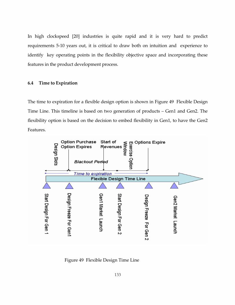
133
In high clockspeed [20] industries is quite rapid and it is very hard to predict
requirements 5‐10 years out, it is critical to draw both on intuition and experience to
identify key operating points in the flexibility objective space and incorporating these
features in the product development process.
6.4 Time to Expiration
The time to expiration for a flexible design option is shown in Figure 49 Flexible Design
Time Line. This timeline is based on two generation of products – Gen1 and Gen2. The
flexibility option is based on the decision to embed flexibility in Gen1, to have the Gen2
Features.
Figure 49 Flexible Design Time Line
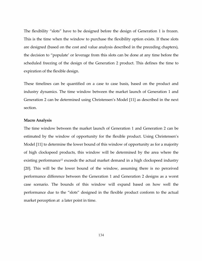
134
The flexibility “slots” have to be designed before the design of Generation 1 is frozen.
This is the time when the window to purchase the flexibility option exists. If these slots
are designed (based on the cost and value analysis described in the preceding chapters),
the decision to “populate’ or leverage from this slots can be done at any time before the
scheduled freezing of the design of the Generation 2 product. This defines the time to
expiration of the flexible design.
These timelines can be quantified on a case to case basis, based on the product and
industry dynamics. The time window between the market launch of Generation 1 and
Generation 2 can be determined using Christensen’s Model [11] as described in the next
section.
Macro Analysis
The time window between the market launch of Generation 1 and Generation 2 can be
estimated by the window of opportunity for the flexible product. Using Christensen’s
Model [11] to determine the lower bound of this window of opportunity as for a majority
of high clockspeed products, this window will be determined by the area where the
existing performance12 exceeds the actual market demand in a high clockspeed industry
[20]. This will be the lower bound of the window, assuming there is no perceived
performance difference between the Generation 1 and Generation 2 designs as a worst
case scenario. The bounds of this window will expand based on how well the
performance due to the “slots” designed in the flexible product conform to the actual
market perception at a later point in time.

135
Figure 50 Boundary for Time to Expiration for Flexibility Strategy
for an established product
A guideline to determine the time to expiration is described in product. The shaded area
shows the approximate performance range of the flexible product. The boundary of the
time to expiration,
TExpMax = T2 – T1 (25)
12 Performance in this section is used from a less rigorous context and would include functional , capacity and performance aspects described in the earlier chapters.
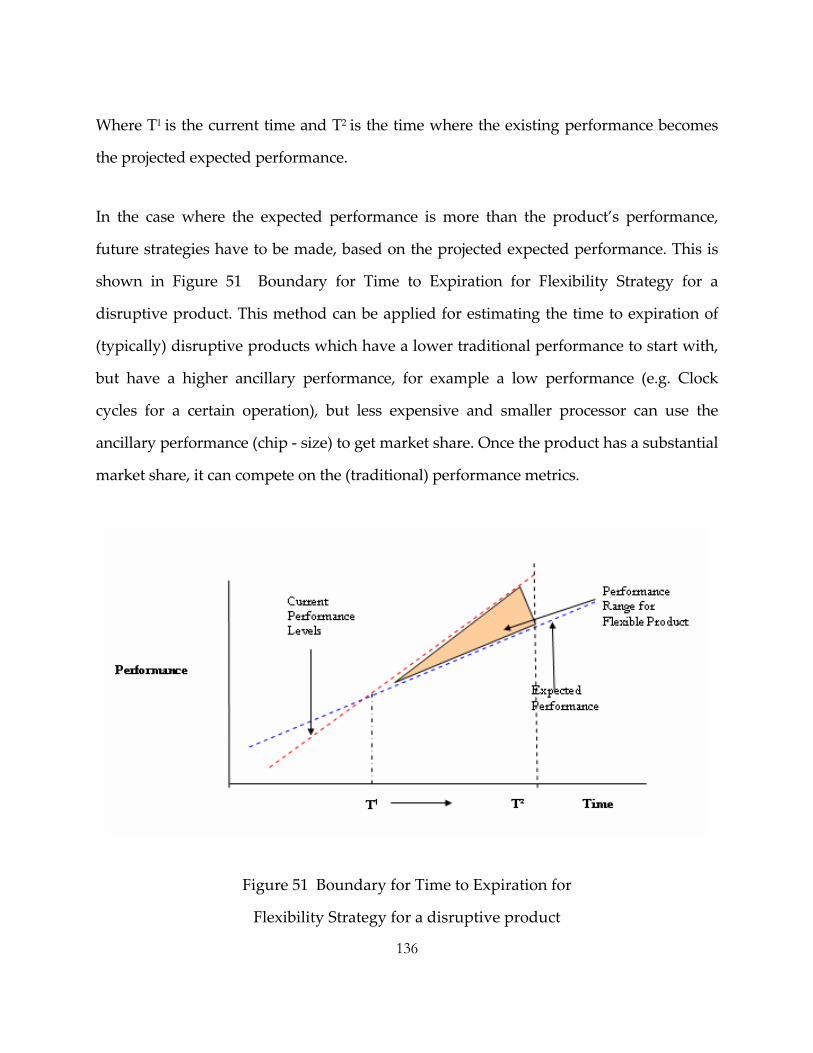
136
Where T1 is the current time and T2 is the time where the existing performance becomes
the projected expected performance.
In the case where the expected performance is more than the product’s performance,
future strategies have to be made, based on the projected expected performance. This is
shown in Figure 51 Boundary for Time to Expiration for Flexibility Strategy for a
disruptive product. This method can be applied for estimating the time to expiration of
(typically) disruptive products which have a lower traditional performance to start with,
but have a higher ancillary performance, for example a low performance (e.g. Clock
cycles for a certain operation), but less expensive and smaller processor can use the
ancillary performance (chip ‐ size) to get market share. Once the product has a substantial
market share, it can compete on the (traditional) performance metrics.
Figure 51 Boundary for Time to Expiration for
Flexibility Strategy for a disruptive product

137
The effective bound of this window would typically be the minimum of the time to
market of the individual performance attributes as described in section 5.3.2 .The actual
range should be dermined factoring in the competitive scenario which would
dynamically make the expected performance front to shift upwards reducing the
window.
The dynamics of this window with respective to the competitive scenario and the
expected performance, can be studied in further detail.
6.5 Cost
The cost of embedding flexibility includes the cost of designing the flexible feature ‘slots’
and the cost of populating these slots at a later point in time. We investigate these cost
from the context of functional , capacity and performance flexibility using the example of
the wireless network application, Application 1, which we used as an example for
“embedding flexibility’ in Chapter 4.
6.5.1 Functional Flexibility
If the flexible objective space cover the whole functional objective space (see Figure 8
Flexibility Design and Objective Space. Adapted from [6]. ), we would have an
unconstrained flexibility where we turn a feature off or on in the complete functional
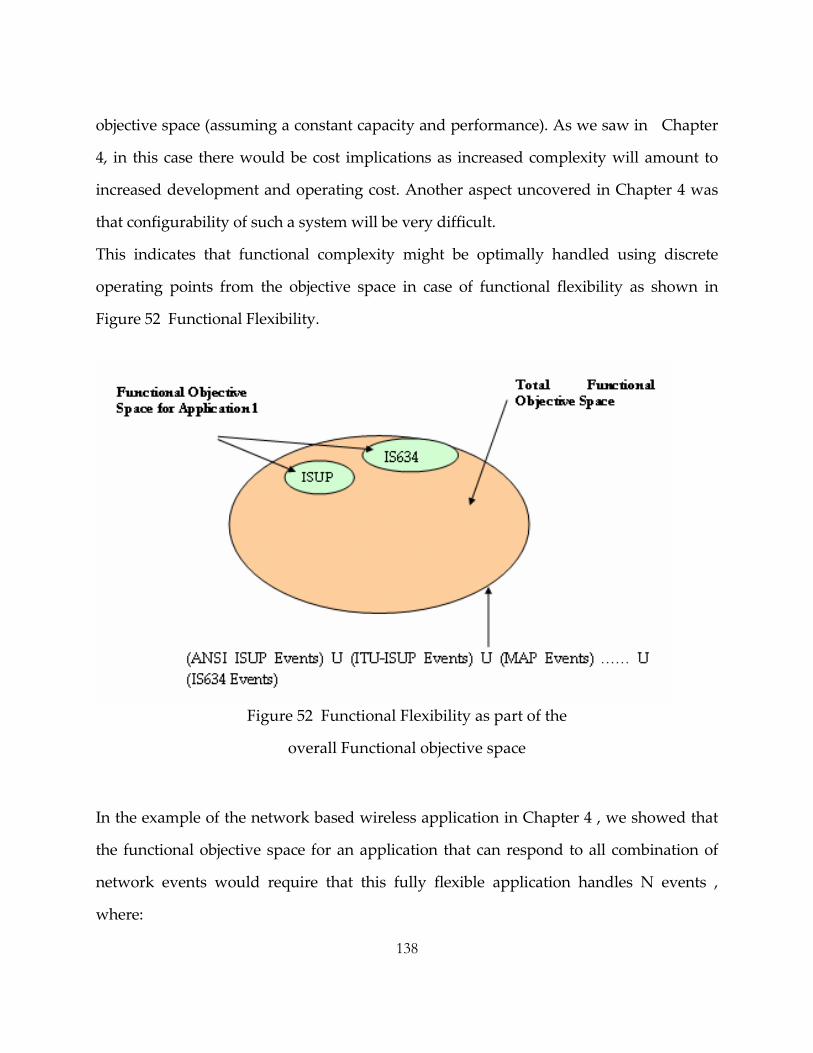
138
objective space (assuming a constant capacity and performance). As we saw in Chapter
4, in this case there would be cost implications as increased complexity will amount to
increased development and operating cost. Another aspect uncovered in Chapter 4 was
that configurability of such a system will be very difficult.
This indicates that functional complexity might be optimally handled using discrete
operating points from the objective space in case of functional flexibility as shown in
Figure 52 Functional Flexibility.
Figure 52 Functional Flexibility as part of the
overall Functional objective space
In the example of the network based wireless application in Chapter 4 , we showed that
the functional objective space for an application that can respond to all combination of
network events would require that this fully flexible application handles N events ,
where:

139
N = (ANSI ISUP Events) U (ITU‐ISUP Events) U (MAP Events) …… U (IS634 Events)
Application 1, described in Chapter 4, handled the IS 634 and ISUP events.
The discrete operating points can be enabled by allowing dynamic addition of diverse
Application State machines (using an architecture similar to that described in Chapter 4),
or enabling some dormant states of an existing state machine. This assumes that flexible
functional operating space can be achieved using the existing interfaces with the
application specific resources. These “slots” have to be designed as part of the flexible
system architecture and can be populated at a later time to achieve functional flexibility.
The cost of implementing functional flexibility is the cost of designing the dormant states
and “slots” for application resources and some amount of testing of potential future
applications.
The cost for populating these slots will be an additional dimension of cost that would be
incurred while activating the feature at a later point of time. In the example of flexible
handset processor described in Chapter 5, this cost will be the cost of activating the
additional cache. In the example of Network based wireless application described in
Chapter 4 , this cost will be the cost of interfacing Application 1 with a SMSC.
6.5.2 Capacity Flexibility
As described in the previous chapter, this dimension depends on the capacity of the
persistent device that gives memory to the state machine – e.g. Enterprise Storage Arrays,
Memory, and Flip Flops. We described in Chapter 4 that how the storage requirement
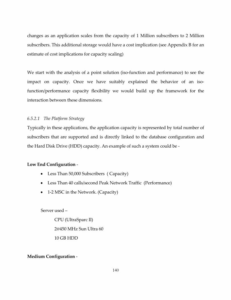
140
changes as an application scales from the capacity of 1 Million subscribers to 2 Million
subscribers. This additional storage would have a cost implication (see Appendix B for an
estimate of cost implications for capacity scaling)
We start with the analysis of a point solution (iso‐function and performance) to see the
impact on capacity. Once we have suitably explained the behavior of an iso‐
function/performance capacity flexibility we would build up the framework for the
interaction between these dimensions.
6.5.2.1 The Platform Strategy
Typically in these applications, the application capacity is represented by total number of
subscribers that are supported and is directly linked to the database configuration and
the Hard Disk Drive (HDD) capacity. An example of such a system could be ‐
Low End Configuration ‐
• Less Than 50,000 Subscribers ( Capacity)
• Less Than 40 calls/second Peak Network Traffic (Performance)
• 1‐2 MSC in the Network. (Capacity)
Server used –
CPU (UltraSparc II)
2@450 MHz Sun Ultra 60
10 GB HDD
Medium Configuration ‐
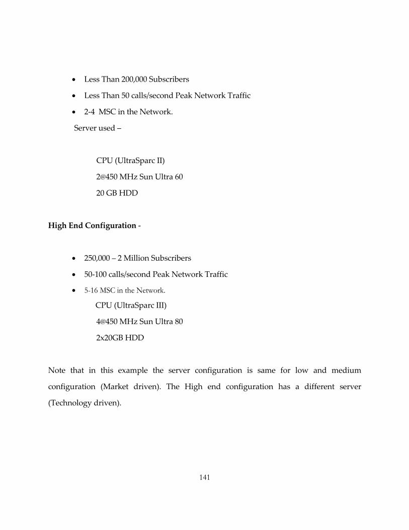
141
• Less Than 200,000 Subscribers
• Less Than 50 calls/second Peak Network Traffic
• 2‐4 MSC in the Network.
Server used –
CPU (UltraSparc II)
2@450 MHz Sun Ultra 60
20 GB HDD
High End Configuration ‐
• 250,000 – 2 Million Subscribers
• 50‐100 calls/second Peak Network Traffic
• 5-16 MSC in the Network.
CPU (UltraSparc III)
4@450 MHz Sun Ultra 80
2x20GB HDD
Note that in this example the server configuration is same for low and medium
configuration (Market driven). The High end configuration has a different server
(Technology driven).

142
Figure 53 Capacity vs. Cost
If we plot the capacity vs. cost as a graph (Figure 53 Capacity vs. Cost) we see that the
cost transitions are discrete (see Appendix B for actual server configuration and cost
data).
The capacity is flexible within Cd1 within the same cost objective, however for Capacity >
Cd1 there is a discontinuity in the objective space ‐ thus indicating the discrete behavior
of Capacity flexibility similar to Functional flexibility. Similar observation is made in
flexibility analysis of communications satellites via orbital reconfigurations and staged
deployment [40]. The discontinuity will intuitively shift left to Cd2 if we increase the
number of functions in the application – increasing the CPU load.

143
6.5.3 Performance Flexibility
As described in the Chapter 4, this dimension depends on the effective bandwidth of
input and output from the system for an I/O constrained application and the CPU
processing bandwidth for processing constrained applications. The processing and I/O
bandwidth is usually limited by the server (or processor board) configuration. A
particular configuration would be able to support capacity flexibility to the limit where its
resources get constrained.
The plot of Performance vs. cost as a graph is shown in Figure 54 Performance vs. Cost.
Figure 54 Performance vs. Cost

144
The Performance is flexible within Pd1 within the same cost objective, however for
Performance > Pd1 there is a discontinuity in the objective space. The point of
discontinuity shifts with increased functionality.
6.6 Conclusion
Methods to determine market volatility, value of the underlying asset and time to
expiration were presented in this chapter.
In order to determine the value of the underlying asset, which is one of the terms needed
for the valuation of flexibility, two approaches are presented: conjoint analysis and
concept engineering. The bounds of time to expiation are explored using Christenson’s
Model [11] and analysis of the timeline of product life cycle based on two generations of a
design. The time to expiration was defined as time window between the start of the first
generation design and the planned design freeze date of the second generation design.
We found that Functional flexibility might be optimally handled using discrete operating
points from the objective space. The cost of implementing functional flexibility is the cost
of designing the dormant states and “slots” for application resources. The cost for
populating these slots constitute to an additional dimension of cost that would be
incurred while activating the feature at a later point of time. Performance flexibility
depends on the effective bandwidth of input and output from the system for an I/O
constrained application and the CPU processing bandwidth for processing constrained
applications. The processing and I/O bandwidth is usually limited by the server (or
processor board) configuration. A particular configuration would be able to support
capacity flexibility to the limit where its resources get constrained. This leads to a discrete

145
change in cost of the system at this boundary. Capacity flexibility, in way similar to
performance flexibility, causes a discrete change in system cost as the database/persistent
device capacity is constrained.

146

147
C h a p t e r 7
Flexibility Strategy and Conclusions
7.1 Introduction
The Flexibility Strategy for a product involves the analysis of the cost and value of
embedding flexibility in a product and selecting the optimum flexible design options.
Once these options have been selected, the portfolio of real options has to be tracked over
time to decide which of these have to be nurtured, exercised or discarded. Nurturing
could involve creating market awareness or demand for a feature that has been designed
in flexible product. Exercising the option would mean implementing these features or
filling the ‘flexible slots’. Discarding the option would mean not exercising the option.
Figure 55 Option Steps for a Flexible Design shows the steps in the comparison of a fixed
design versus a flexible design. The cost of designing flexibility or the ‘flexible slots’ is
determined by the cost of the steps α , β and γ . These steps could be combined as one for
products where these options cannot be separately purchased.. The cost of implementing
flexibility or populating the flexible slots is determined by the cost of step δ.
If the value of the module described in Figure 55 Option Steps for a Flexible Design is
VCM, where:
V is the value for the product configuration C, for the party M.

148
Figure 55 Option Steps for a Flexible Design
M can be customer “C” or enterprise “E” (for this analysis).
C is the product configuration, which can be :
0 : without the module
1: with integrated module
α :with reserved resources for module
149
β : with interfaces with module
γ : with designed module
δ : with implemented module
Value of the module to the customer, Vmod can be expressed as:
Vmod = V1C – V0C (26)
The cost of the module to the Enterprise is:
For fixed design option, the cost to the enterprise CFixed, for two generations of the
product is ‐
CFixed = C0E + C1E (27)
For the flexible design option, the cost to the enterprise is CFlex,
CFlex = CαE + Cβ
E + CγE + Cδ
E (28)
The baseline module (first generation only) is recommended when:
Vmod < Minimum(CFixed , CFlex ) (29)
Fixed design is recommended when:
CFixed < Minimum (CFlex , Vmod) (30)
Flexible product strategy is recommended when:

150
CFlex < Minimum (CFixed , Vmod) (31)
Once Flexible product strategy is found to be the optimal strategy, for different features
or ‘modules’, we need to choose the portfolio of options which are optimal and which we
would then embed in the product architecture. These options are for different flexibility
features.
7.2 Option Analysis
To make the optimal decision, we have to choose an optimal set of design options from
the flexibility design vector Dp (Eq. 8). This vector has an associated cost Cf (Eq. 9) along
with an associated value of embedding flexibility as computed using the Real Options
approach, Vf (Eq. 11). Figure 56 Flexibility Design Space presents the possible Dp
vectors, each with an associated Cf and Vf values. The Y axis represents the cost of
flexibility, and the X axis its value.
The choice of flexibility options is different from the choice of financial options because
the choice of design options would be done at the time of “embedding” flexibility. Once
the initial set is chosen, we are restricted to this portfolio of options for all future product
strategies. The choice initial set of design vectors would depend on the decision maker’s
utility profile and external constraints. We provide the recommendation for choosing
these options under three different scenarios.
7.2.1 Rate of Return Scenario

151
In this scenario, the option set with maximum rate of return is chosen, irrespective of
other factors. All the points that fall above the y=x line in Figure 56 Flexibility Design
Space, have a cost to value ratio greater than 1, and therefore should not be considered as
valid flexibility design options.
Let the Cost Vector Cv,
Cv = {C0 , C1 ….Cn } (32)
Where,
n is the number of design options,
Ci is the cost Cf of the ith design vector.
The Design Option Vector Dv,
Dv = {D0 , D1 ….Dn } (33)
Where,
n is the number of design options,
Di is ith design vector.
The Option Value Vector Vv,
Vv = {V0 , V1 ….Vn } (34)
Where,
n is the number of design options,

152
Vi is the real‐option value of the ith design vector.
The strategy for maximizing the rate of return scenario would involve choosing the
design options from the Design Option Vector, with the maximum return ratio Rmax
Ramax can be also be represented by the minimum slope of the line that corresponds to a
valid Design Vector , represented by the normalized value and cost as shown in Figure 56
Flexibility Design Space for maximizing rate of return .
The optimal design options are shown in the figure Figure 56 Flexibility Design Space for
maximizing rate of return , which include the design options that have the rate of return
between Rmax and Rc , which is the cut off rate of return value.
vivii
i CCVVVCMinR ∈∀∈∀= ,),(max (35)
Thus the Flexibility Design Option vector, Dfv can be defined as
Dfv = {D0 , D1 ….Dm } ∀Dk ∈Dfv , Rc> Ck /Vk > Rmax (36)
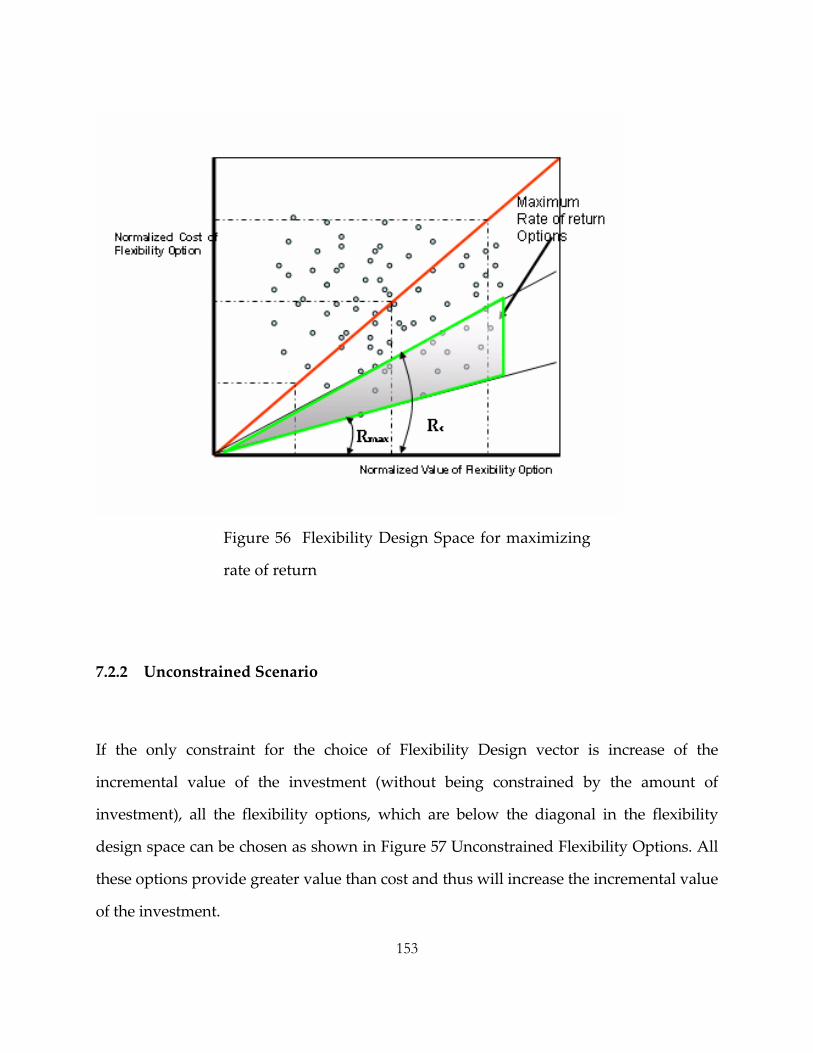
153
Figure 56 Flexibility Design Space for maximizing
rate of return
7.2.2 Unconstrained Scenario
If the only constraint for the choice of Flexibility Design vector is increase of the
incremental value of the investment (without being constrained by the amount of
investment), all the flexibility options, which are below the diagonal in the flexibility
design space can be chosen as shown in Figure 57 Unconstrained Flexibility Options. All
these options provide greater value than cost and thus will increase the incremental value
of the investment.

154
Net Incremental value of Investment is Inv where :
Inv = (C∑ =
n
i 0 i ‐Vi ) (37)
To maximize Inv , we have to choose the Design vectors Dv from the Design Option
vector , where, Vi > Ci
Thus the Flexibility Design Option vector, Dfv can be defined as
Dfv = {D0 , D1 ….Dm }, ∀Dk ∈Dfv , (Vk –Ci ) > 0 (38)
Where m <= n, the total number of design options. This set is shown in Figure 57
Unconstrained Flexibility Options.
In the unconstrained scenario, some of the options which have a marginally higher cost
than value, but have a high volatility, can also be chosen as the value of such options can
change favorably in the future.

155
Figure 57 Unconstrained Flexibility Options
7.2.3 Constrained Scenario
In the constrained scenario, there could be investment constraints. These constraints can
be in the form of limit on the total investment, maximum investment for a single design
option, among others. One strategy is to select the optimum design options, with a total
investment limit. The portfolio of optimum design options are selected from the Design
Vector, based on their individual rate of return. Design options that have the maximum
rate of return are selected till the total cost exceeds the maximum investment limit.
156
7.3 Portfolio of Real Options
Using the cost and value(s) of embedding flexibility, we recommend a Portfolio of Real
Options based Flexibility Strategy in this section, which is based on earlier work by T.A
Luehrman [25].
The main concept of this approach is that once we ascertain the value, cost and the
volatility of the optimal design front identified in the previous section, we have to devise
a strategy to activate these options at a future point of time.
We can make the flexibility strategy based on the value‐to‐cost and volatility dimensions
that exist at a given point of time. The first in the chain of this option is the value of the
optimal design Pareto front as a whole. This will drive the decision to invest in the R&D
and design cost for this portfolio. This decision would be linked with “activating” the
individual features at a point time in the future. As we mentioned in the last section , the
design parameters optimum design parameters would change with time and some of
these would turn out to be really profitable , others not. Doing this analysis would help
us to determine the investment we could make in “nurturing” a particular type of design
option, or “write off” another. The nurturing costs could include advertising expense,
costs to make strategic alliances etc. The key point of this method is to see the portfolio of
optimal design parameters identified in the previous section as a chain of options rather
than static NPV based decision.
157
7.4 Conclusion
.
The flexibility of a system is its ability to meet a changing set of requirements after it has
been fielded under new modes of use or changes in its environment. The purpose of this
research was to provide a framework for estimating the value of embedding flexibility in the
design of a system and to recommend a strategy based on this value that would enable us
to make decisions to choose the flexible attributes and the resources to invest in these
attributes for optimum value capture.
Real Options analysis was used to model the payoffs associated with the flexible design
options in the face of uncertainty. This approach is more suitable than the Net Present
Value (NPV) based analysis which assumes a static view of the market, when in reality,
uncertainty and investment choices exist together and these choices are spread over time.
As uncertainty resolves, downside losses can be avoided by not investing more funds
into projects which have poor performance.
The Real option Analysis of Flexibility, which was explored in detail in this thesis can be
summarized using de Weck’s general real option reasoning framework [40] as shown in
Figure 58 General Real option reasoning Framework (adapted from [40]).

158
Figure 58 General Real option reasoning Framework (adapted from [40])
7.5 Future Work
Beyond the work done in this thesis, research avenues could include more accurate
quantitative methods for computing volatility for flexible design variants in the face of
uncertainty for breakthrough products. Furthermore, a comprehensive methodology

159
could be developed for determining the bounds of the expiration time for exercising
flexible design options.
The comparison of fixed and flexible design options which was done in this thesis can be
extended to develop quantitative models of the tradeoffs between the flexibility design
costs and flexibility implementation costs and how moving the costs from design to
implementation , affects the relative attractiveness of a flexible design option as compared
to a fixed design.
The tradeoff between the flexibility dimensions ‐ functional flexibility, capacity flexibility
and performance flexibility can be quantitatively analyzed within given resource
constraints.

160
161
A p p e n d i x A
GSM, TDMA & CDMA Overview
GSM – Global System Mobile
Frequency Bands
GSM operates in three frequency bands – Cellular, PCN and PCS. The frequency
allocations in these bands are –
Cellular ‐ 890‐915MHz and 935‐960MHz
PCN – 710‐785 MHz and 1805‐1880MHz
PCS ‐ 1850‐1910 MHz and 1930‐1990MHz
The first half of the bands is used for transmitting and the other half is used for
receiving.
Modulation Scheme
Each band is subdivided into 124 FDM channels spaced 200KHz apart. Each of these
carrier frequencies is further subdivided into .577 ms TDM channels which are used for
control messaging and voice traffic. The traffic channel burst of 156 bits of data has two
blocks of 57 bit data and a 26 bit training sequence.
TDMA – IS‐136
162
Frequency Bands
IS‐136 operates in the Cellular and PCS frequency bands (900 and 1900 MHz).
Modulation Scheme
TDMA uses differential quadrature phase shift keying and provides an across air bit rate
of 48.6 Kbps. The TDMA frame is of 40 mS duration with six 6.67 ms slots per frame. Two
slots are allocated for full rate voice channel.
CDMA – IS‐95
Frequency Bands
Uses AMPS band (Analog). 824‐849 MHz for uplink and 869‐894 MHz for downlink.
1.2 MHz bands with frequency spacing of 45 MHz.
Modulation Scheme
Code Division Multiple Access, uses a spread spectrum modulation scheme. The signal is
spread using a pseudo random noise sequence. Offset Quadrature Phase Shift Keying
(OPSK) is used for reverse channel and Quadrature Phase Shift Keying (QPSK) for
forward channels.

163
A p p e n d i x B
Cost Implication for Capacity Scaling of Database Applications The Capacity scaling considered here is based on the size of the storage (hardware cost)
and the database license (software). These costs are based on the pricing information
available in the public domain at the time this appendix was written. The hardware and
database configurations are based on the analysis of Application 1 storage requirement
described in Chapter 5.
CAPACITY
(SUBSCRIBERS)
CONFIGURATION COST ($) TOTAL COST ($)
100,000 – 500,000 Hardware Sun Fire B100s SPARC Blade Server w/1‐GB Memory Database In Memory Database (1GB limit)
6,590
10,000
16,590
500,000 – 1 Million Hardware 2 x Sun Fire B100s SPARC Blade Server w/1‐GB Memory
8,385
18,385
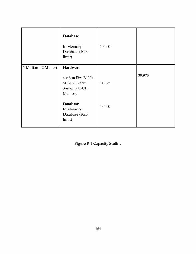
164
Database In Memory Database (1GB limit)
10,000
1 Million – 2 Million Hardware 4 x Sun Fire B100s SPARC Blade Server w/1‐GB Memory Database In Memory Database (2GB limit)
11,975
18,000
29,975
Figure B‐1 Capacity Scaling

165
Bibliography 1. J. Saleh, D. Hastings, D. Newman. Flexibility in system design and implications for
aerospace systems, Acta Astronautica, September 2002. 2. E. Fricke, A. Schulz, S. Wenzel, H. Negele. Design for Changeability, of Integrated
Systems within a Hyper‐Competitive Environment, Proceedings of INCOSE Colorado Front Range Chapter Regional Conference, 2000, Denver.
3. O. de Weck, D. Chang. Architecture Trade Methodology for LEO Personal
Communication Systems, AIAA 2002‐1866, Montreal, Canada, May 12‐15 2002. 4. E.F. Crawley. ESD.34 System Architecture, Massachusetts Institute of Technology,
Cambridge Massachusetts. 5. Bob Liebeck. Design of Subsonic Transports, ESD.34 System Architecture,
Massachusetts Institute of Technology, Cambridge Massachusetts.
6. O. de Weck, K. Wilcox. ESD.77 Massachusetts Institute of Technology, Cambridge Massachusetts.
7. R. de Neufville, J Clark, F.R Field. Real Options 2 , Engineering Systems Analysis for
Design , Massachusetts Institute of Technology, Cambridge Massachusetts.
8. Geoffrey A Moore. Crossing the Chasm, Harper Collins, 1999. 9. Crawley, de Weck. 2003 – NASA HQ presentation, Massachusetts Institute of
Technology, Cambridge Massachusetts. 10. Rebecca M. Henderson and Kim B. Clark. The Reconfiguration of Existing Product
Technologies and the Failure of Established Firms, Administrative Science Quarterly, 1990, vol. 35.
11. Christensen, CM. The Innovator’s Dilemma, Harper Business, New York, ISBN 0‐06‐
662069‐4.

166
12. Moise Solomon, J. Utterback. Software Defined Radio: A System Engineering View of
Platform Architecture and Market Diffusion, SM Thesis, Massachusetts Institute of Technology, Cambridge Massachusetts.
13. Third Generation Wireless Network Evolution in North America – Yankee Group
Report 2000. 14. Javier P, Gonzalez‐Zugasti, Kevin N. Otto, John D. Baker. Assessing value in
platformed product family design, Massachusetts Institute of Technology, Cambridge Massachusetts.
15. Dixit A, Pindyck R (1994). Investment under uncertainty. Princeton University Press,
Princeton. 16. Timothy Luehrman. Investment Opportunities as Real Options‐Getting started on the
numbers, HBR July‐August 1998. 17. Martha Amram, N. Kulatilaka.. Real Options, HBS School Press. 18. Michael A Cusumano et al. Strategic Maneuvering and Mass‐Market Dynamics. 19. T.A. Luehrman. Strategy as a portfolio of Real Options; Harvard Business Review
September‐October 1998. 20. Charles H Fine. Clockspeed : Winning Industry Control in the Age of Temporary
Advantage, Persues Books , Reading Massachusetts. 21. Harry E. Cook. Fundamentals of Value Benchmarking, SAE Technical Paper, 1996. 22. Paul E. Green and Yoram Wind. New way to measure consumers judgement,
Harvard Business Review July‐August 1975. 23. John R. Hauser and Don Clausing. The House of Quality, Harvard Business Review
May‐June, 1998.

167
24. S. Shiba, D. Walden. Four Practical Revolutions in Management, Center of Quality of Management , Cambridge MA.
25. T.A. Luehrman. Strategy as a portfolio of Real Options; Harvard Business Review
September‐October 1998. 26. C. Haubelt, J. Teich, K. Richter, R. Ernst. System Design for Flexibility, Proceedings of
Design, Automation and Test in Europe, Paris, France, March 2002. 27. M. Gaynor, S. Bradner, M. Iansiti, H.T. Kung. The Real Options approach to
Standards for Building Network‐based Services. 28. Jim Doyle et al: Power Optimization Challenges in Next Generation Handsets,
Portable Power Systems, National Semiconductors. 29. Shiv Putcha. Asia‐Pacific Wireless/Mobile Forecast, 2Q03, Yankee Group Report June
2003. 30. John R. Hauser and Don Clausing. The House of Quality , Harvard Business Review
May‐June, 1998 31. 3D Gaming Market Study – Penton Digital Media Research. 32. Prithviraj Banerjee, et. al. System and methods for distributed telecommunication
applications for the public switched telephone network and the public land mobile network, US Patent Application 20020048360, April 2002.
33. Fischer Black and Myron Scholes. The Pricing of Options and Corporate Liabilities.ʹ
Journal of Political Economy 81 (May 1973), pp. 637‐654. 34. Chris Magee, Dan Fry. System Engineering ESD.33J, Massachusetts Institute of
Technology, Cambridge, Massachusetts. 35. Ed Crawley, Olivier de Weck. System Architecture ESD 34.J, Massachusetts Institute
of Technology, Cambridge, Massachusetts.

168
36. J. Utterback. Mastering the Dynamics of Innovation, Harvard Business School Press,
1996. 37. Travis Russel. Signaling System #7, Third Edition, Mc Graw Hill Telecom. 38. Smith, Collins. 3G Wireless Networks . Mc Graw Hill Telecom. 39. Adam Borison. Real option Analysis: Where are the Emperor’s clothes? (Draft),
Stanford University. 40. O. L. de Weck, R. de Neufville, Mathieu Chaize. Enhancing the economics of
communications satellites via orbital reconfigurations and staged deployment, AIAA‐2003‐6317.
41. Robert Ware, Frank Lad. Approximating the distribution for Sums of Products of
Normal Variables, University of Canterbury, New Zealand.
.


