
SA-1
Probabilistic Robotics
Probabilistic Motion and Sensor Models
Some slides adopted from: Wolfram Burgard, Cyrill Stachniss,
Maren Bennewitz, Kai Arras and Probabilistic Robotics Book
2
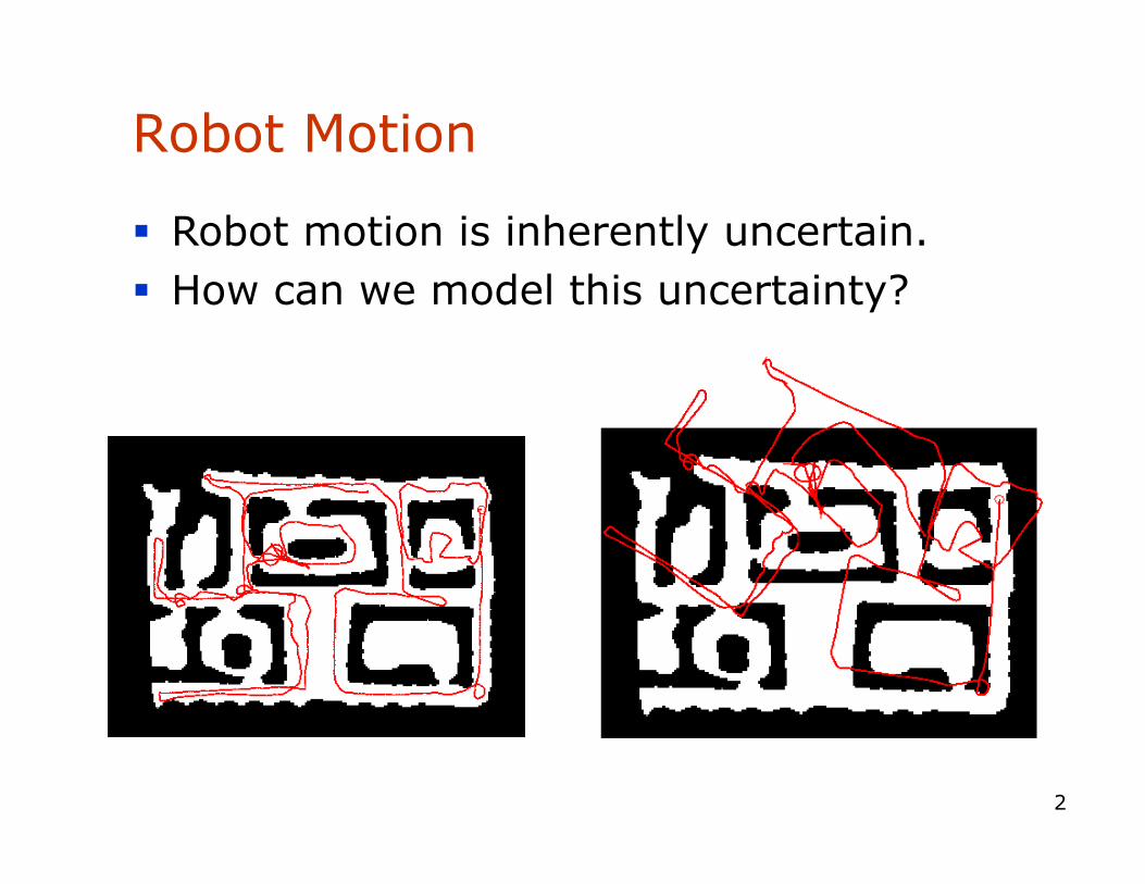
Robot Motion
Robot motion is inherently uncertain. How can we model this uncertainty?
3
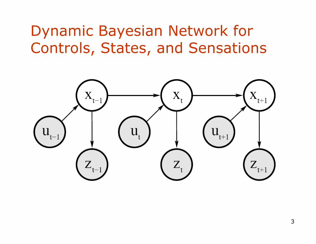
Dynamic Bayesian Network for Controls, States, and Sensations
4
Probabilistic Motion Models
• To implement the Bayes Filter, we need the transition model p(x | x’, u).
• The term p(x | x’, u) specifies a posterior probability, that action u carries the robot from x’ to x.
• In this section we will specify, how p(x | x’, u) can be modeled based on the motion equations.

5
Coordinate Systems • In general the configuration of a robot can be
described by six parameters.
• Three-dimensional Cartesian coordinates plus three Euler angles pitch, roll, and tilt.
• Throughout this section, we consider robots operating on a planar surface.
The state space of such systems is three-dimensional (x,y,θ).
6
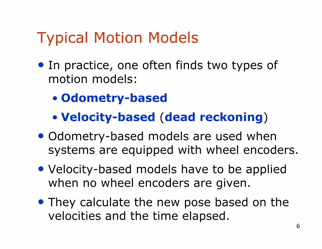
Typical Motion Models
• In practice, one often finds two types of motion models:
• Odometry-based
• Velocity-based (dead reckoning)
• Odometry-based models are used when systems are equipped with wheel encoders.
• Velocity-based models have to be applied when no wheel encoders are given.
• They calculate the new pose based on the velocities and the time elapsed.

7
Example Wheel Encoders
These modules require +5V and GND to power them, and provide a 0 to 5V output. They provide +5V output when they "see" white, and a 0V output when they "see" black. These disks are
manufactured out of high quality laminated color plastic to offer a very crisp black to white transition. This enables a wheel encoder sensor to easily see the transitions.
Source: http://www.active-robots.com/

8
Dead Reckoning
• Derived from “deduced reckoning.” • Mathematical procedure for
determining the present location of a vehicle.
• Achieved by calculating the current pose of the vehicle based on its velocities and the time elapsed.
9
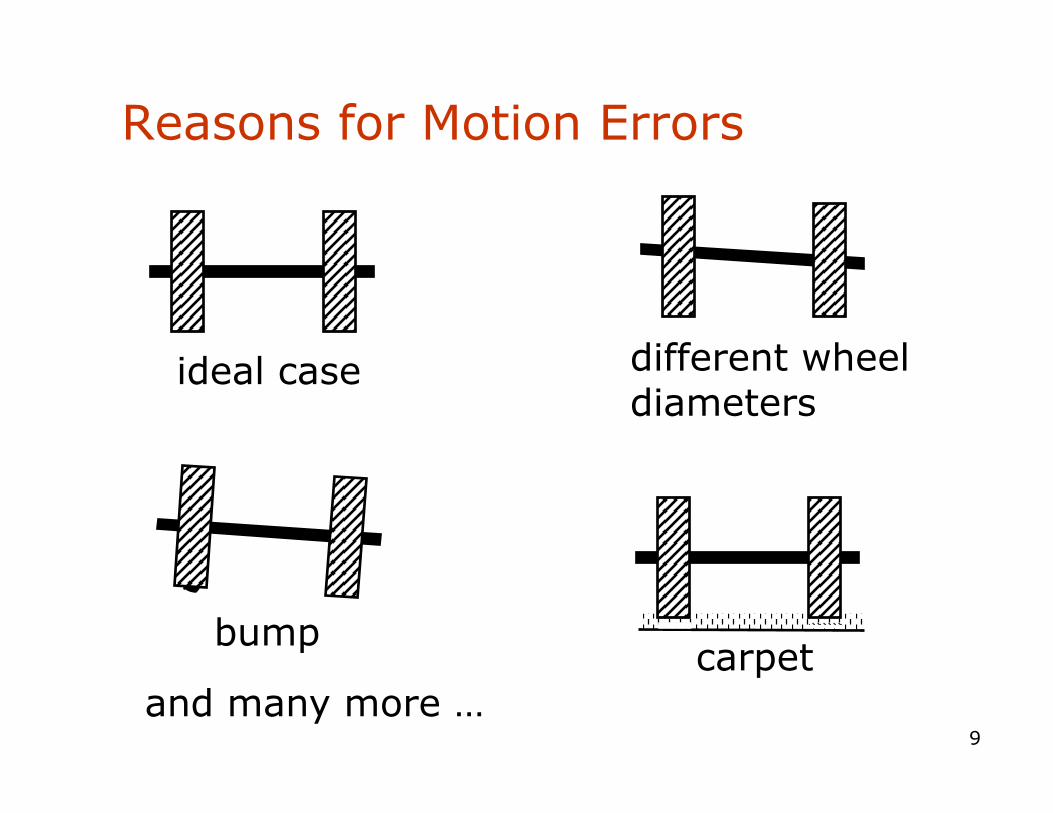
Reasons for Motion Errors
bump
ideal case different wheel diameters
carpet and many more …

Odometry Model
• Robot moves from to .
• Odometry information .
11
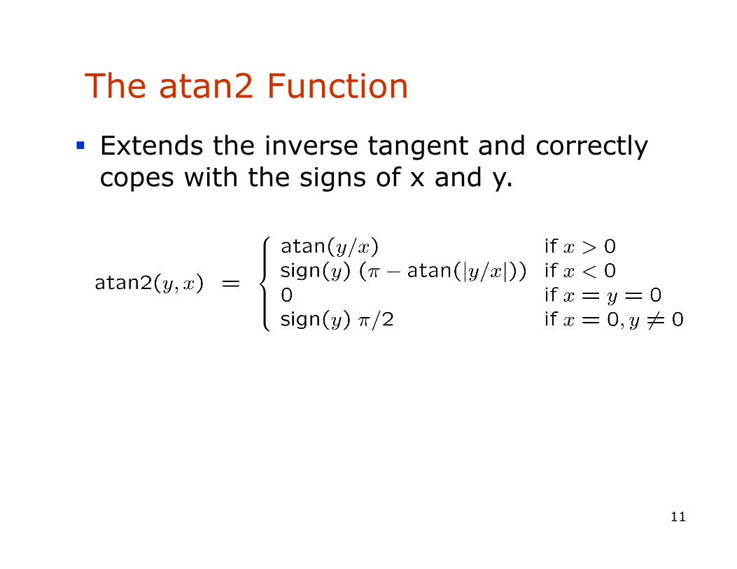
The atan2 Function
Extends the inverse tangent and correctly copes with the signs of x and y.

Noise Model for Odometry
• The measured motion is given by the true motion corrupted with noise.
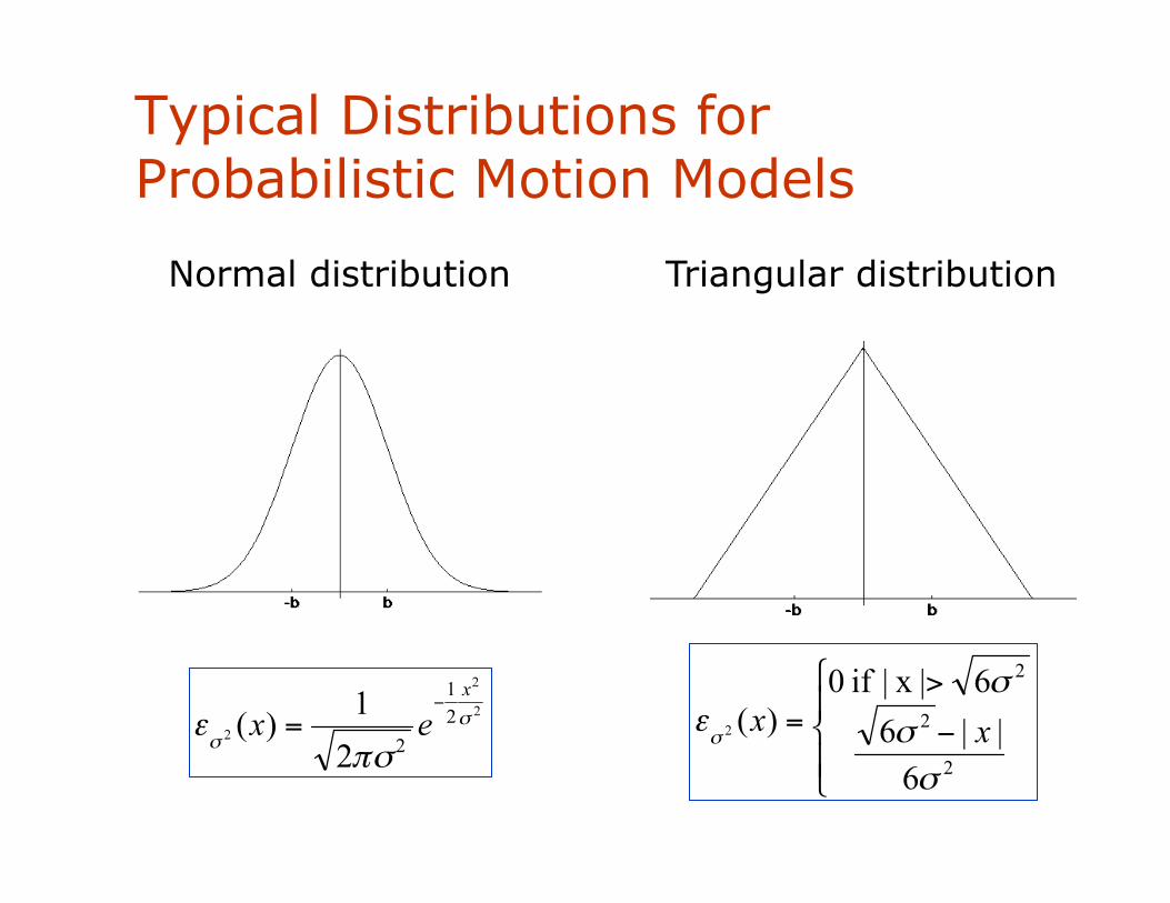
Typical Distributions for Probabilistic Motion Models
Normal distribution Triangular distribution
14
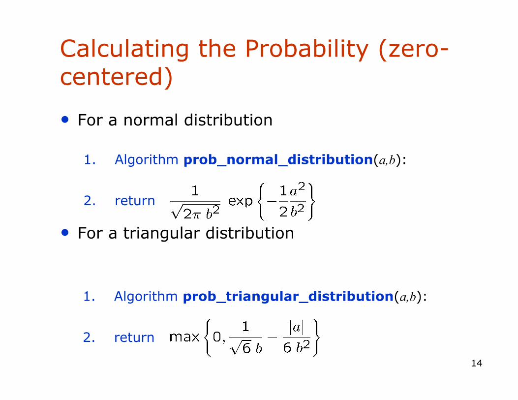
Calculating the Probability (zero-centered)
• For a normal distribution
• For a triangular distribution
1. Algorithm prob_normal_distribution(a,b):
2. return
1. Algorithm prob_triangular_distribution(a,b):
2. return

15
Calculating the Posterior Given x, x’, and u 1. Algorithm motion_model_odometry(x,x’,u)
2.
3.
4.
5.
6.
7.
8.
9.
10.
11. return p1 · p2 · p3
odometry values (u)
values of interest (x,x’)
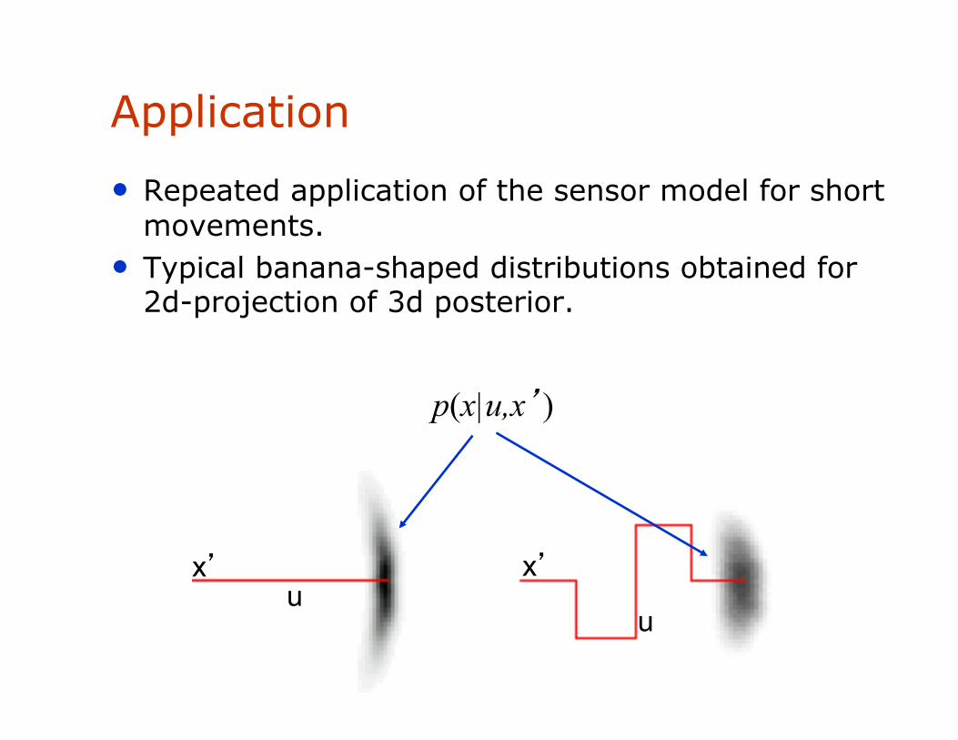
Application
• Repeated application of the sensor model for short movements.
• Typical banana-shaped distributions obtained for 2d-projection of 3d posterior.
x’ u
p(x|u,x’)
u
x’
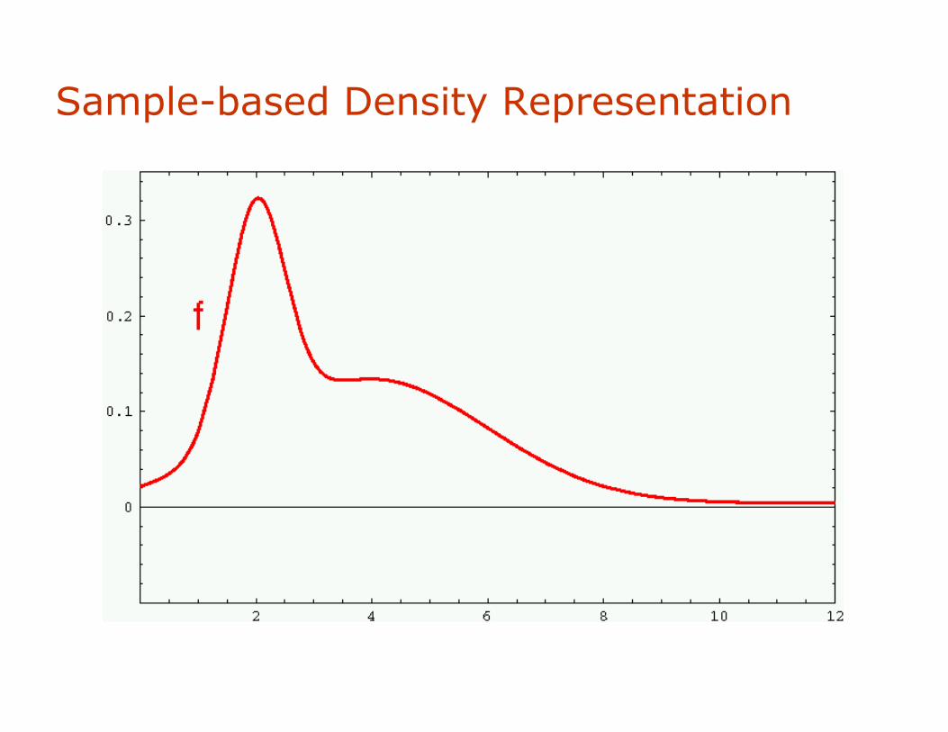
Sample-based Density Representation
18
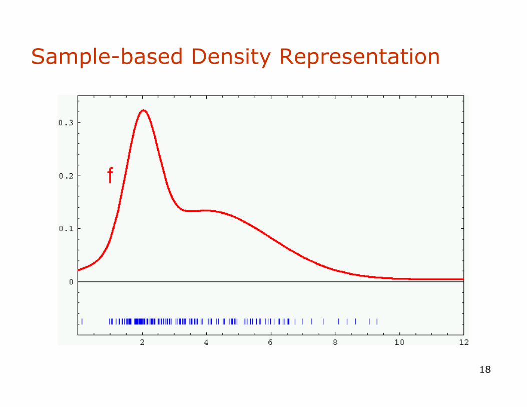
Sample-based Density Representation

19
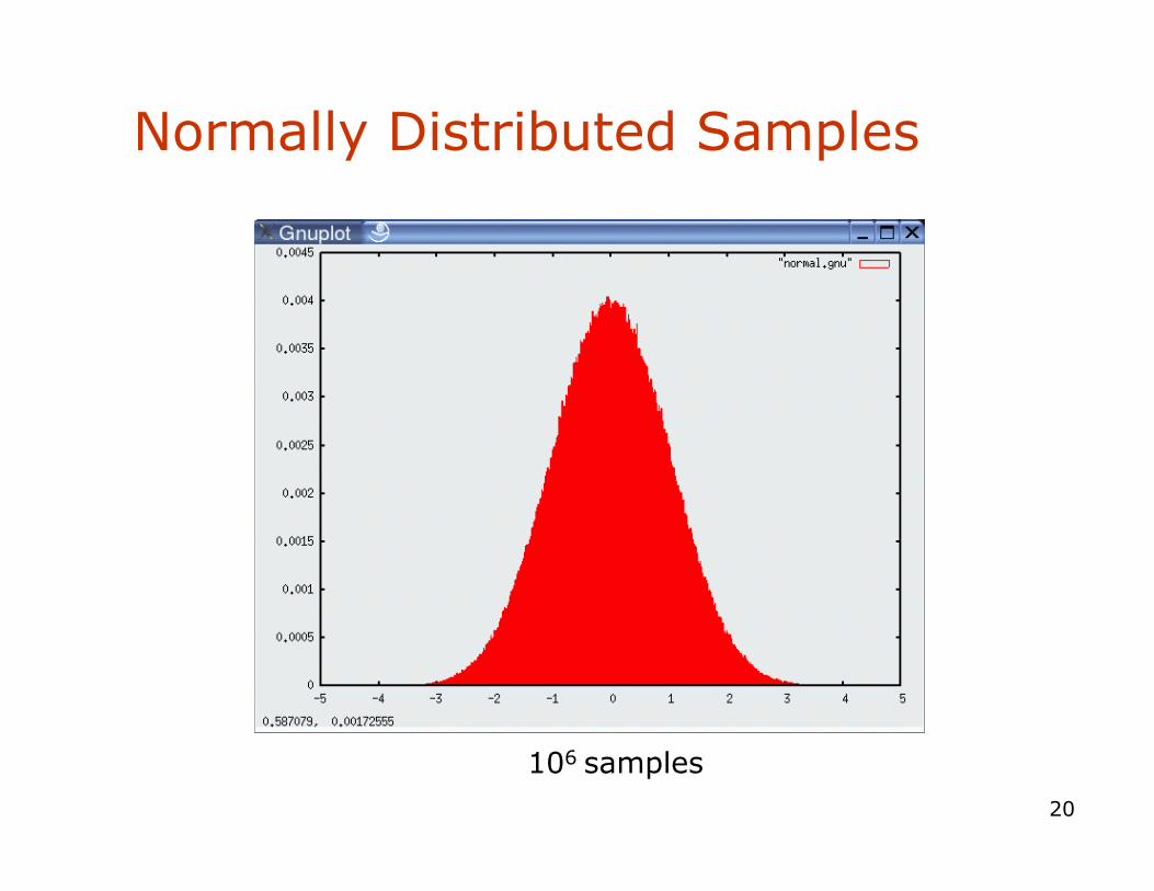
How to Sample from Normal or Triangular Distributions?
• Sampling from a normal distribution
• Sampling from a triangular distribution
1. Algorithm sample_normal_distribution(b):
2. return
1. Algorithm sample_triangular_distribution(b):
2. return
20
Normally Distributed Samples
106 samples

21
For Triangular Distribution
103 samples 104 samples
106 samples 105 samples
22
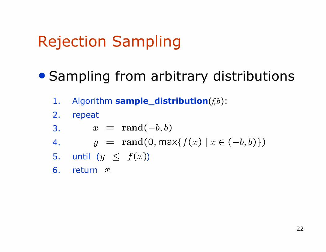
Rejection Sampling
• Sampling from arbitrary distributions
1. Algorithm sample_distribution(f,b):
2. repeat
3.
4.
5. until ( )
6. return

23
Example
• Sampling from

Sample Odometry Motion Model 1. Algorithm sample_motion_model(u, x):
1.
2.
3.
4.
5.
6.
7. Return
sample_normal_distribution
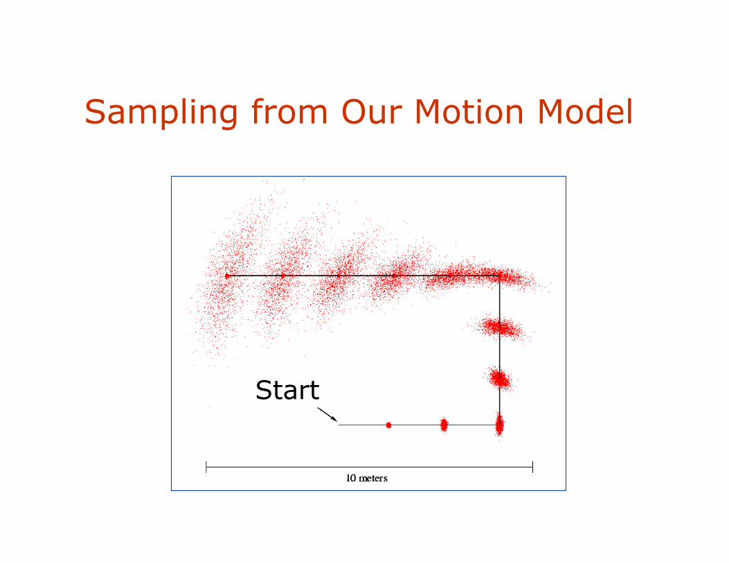
Sampling from Our Motion Model
Start

Examples (Odometry-Based)

Map-Consistent Motion Model
≠ Approximation: In the presence of the map : samples cannot be at occupied cells
33
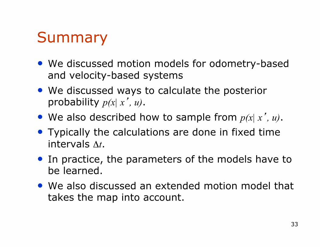
Summary
• We discussed motion models for odometry-based and velocity-based systems
• We discussed ways to calculate the posterior probability p(x| x’, u).
• We also described how to sample from p(x| x’, u). • Typically the calculations are done in fixed time
intervals Δt. • In practice, the parameters of the models have to
be learned.
• We also discussed an extended motion model that takes the map into account.

34
Sensors for Mobile Robots
• Contact sensors: Bumpers
• Internal sensors • Accelerometers (spring-mounted masses) • Gyroscopes (spinning mass, laser light) • Compasses, inclinometers (earth magnetic field, gravity)
• Proximity sensors • Sonar (time of flight) • Radar (phase and frequency) • Laser range-finders (triangulation, tof, phase) • Infrared (intensity)
• Visual sensors: Cameras
• Satellite-based sensors: GPS

35
Proximity Sensors
• The central task is to determine P(z|x), i.e., the probability of a measurement z given that the robot is at position x.
• Question: Where do the probabilities come from? • Approach: Let’s try to explain a measurement.

36
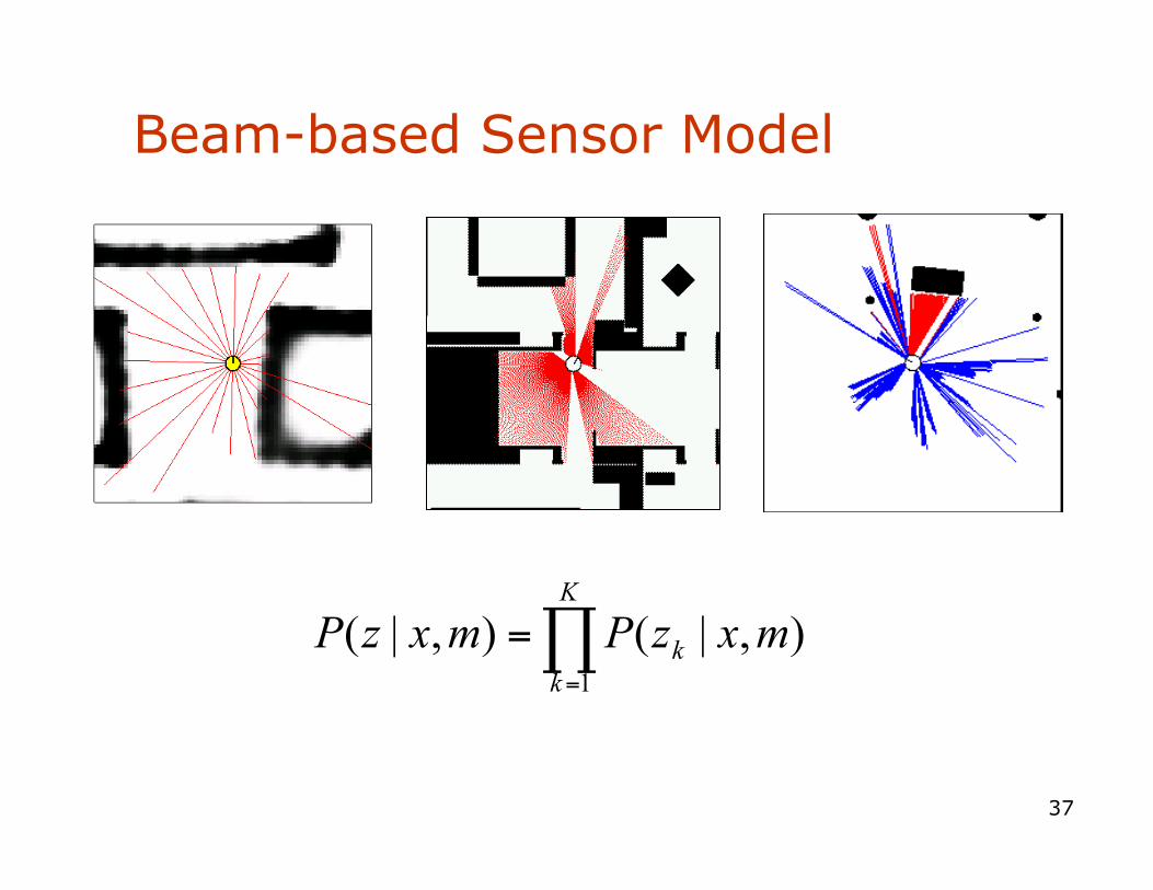
Beam-based Sensor Model
• Scan z consists of K measurements.
• Individual measurements are independent given the robot position.
37
Beam-based Sensor Model
38
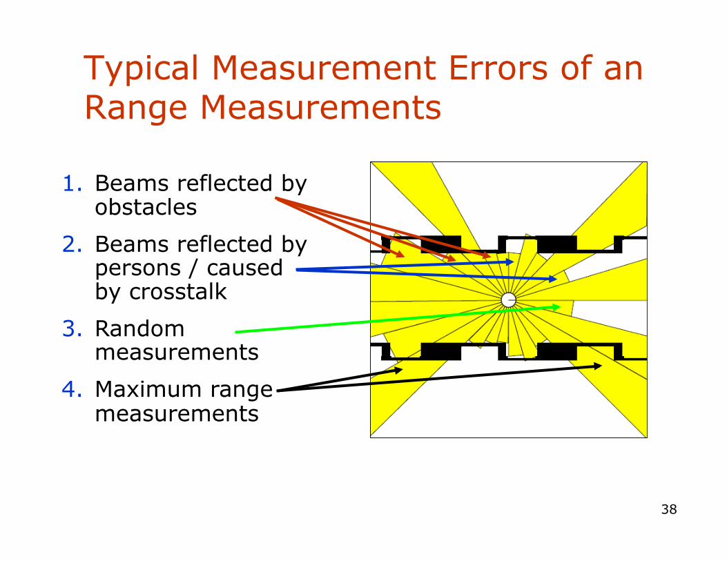
Typical Measurement Errors of an Range Measurements
1. Beams reflected by obstacles
2. Beams reflected by persons / caused by crosstalk
3. Random measurements
4. Maximum range measurements

39
Proximity Measurement
• Measurement can be caused by … • a known obstacle. • cross-talk. • an unexpected obstacle (people, furniture, …). • missing all obstacles (total reflection, glass, …).
• Noise is due to uncertainty … • in measuring distance to known obstacle. • in position of known obstacles. • in position of additional obstacles. • whether obstacle is missed.
40
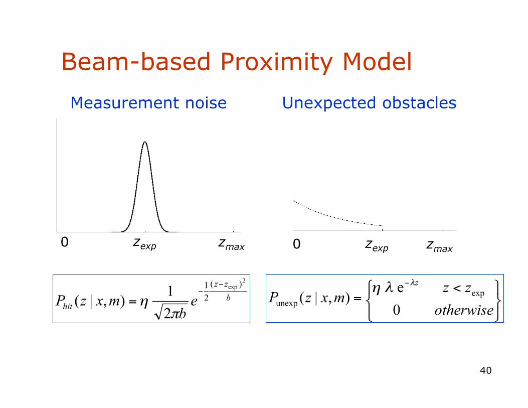
Beam-based Proximity Model
Measurement noise
zexp zmax 0
Unexpected obstacles
zexp zmax 0
41
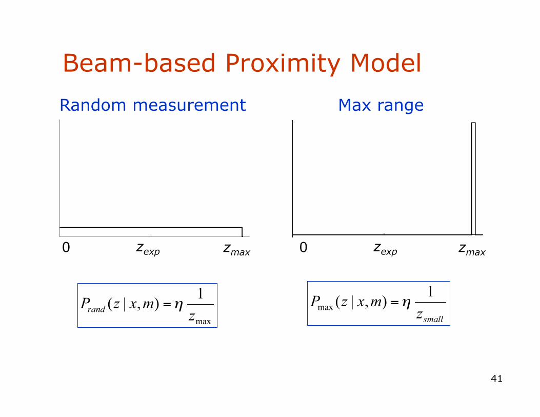
Beam-based Proximity Model
Random measurement Max range
zexp zmax 0 zexp zmax 0
42
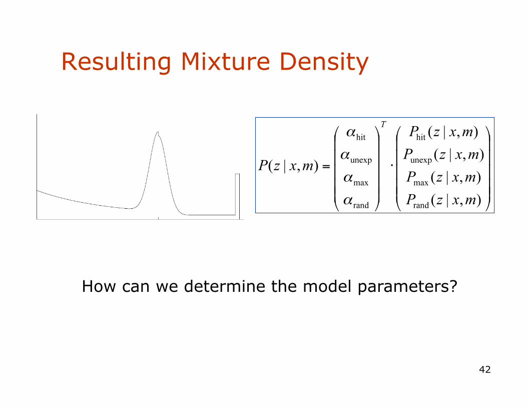
Resulting Mixture Density
How can we determine the model parameters?
43
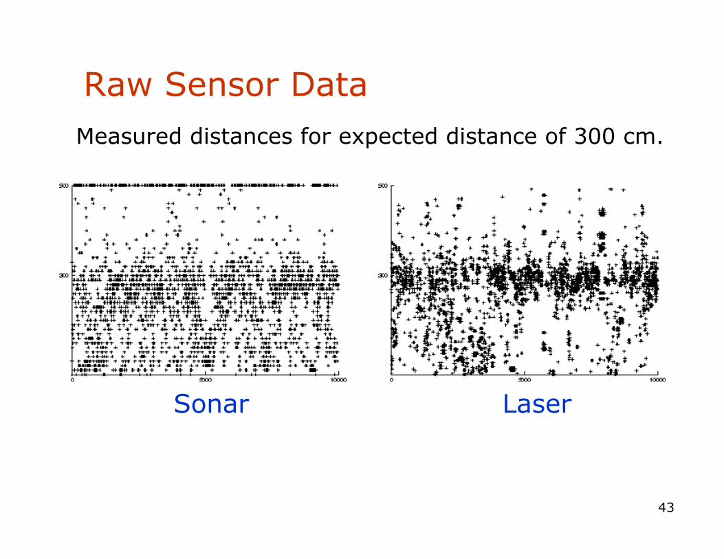
Raw Sensor Data Measured distances for expected distance of 300 cm.
Sonar Laser

44
Approximation
• Maximize log likelihood of the data
• Search space of n-1 parameters. • Hill climbing • Gradient descent • Genetic algorithms • Expectation maximization • ML estimate of the parameters
• Deterministically compute the n-th parameter to satisfy normalization constraint.

45
Approximation Results
Sonar
Laser
300cm 400cm
46
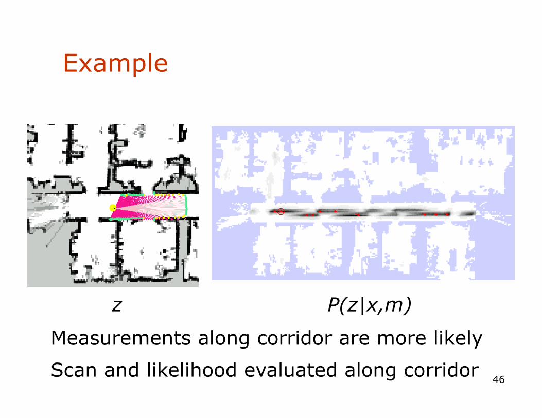
Example
z P(z|x,m)
Measurements along corridor are more likely
Scan and likelihood evaluated along corridor

53
Summary Beam-based Model
• Assumes independence between beams. • Justification? • Overconfident!
• Models physical causes for measurements. • Mixture of densities for these causes. • Assumes independence between causes. Problem?
• Implementation • Learn parameters based on real data. • Different models should be learned for different angles at
which the sensor beam hits the obstacle. • Determine expected distances by ray-tracing. • Expected distances can be pre-processed.

54
Scan-based Model
• Beam-based model is … • not smooth for small obstacles and at
edges. • not very efficient. • Small change in pose – large change in likelihood
• Idea: Instead of following along the beam, just check the end point.

55
Scan-based Model
• Probability is a mixture of … • a Gaussian distribution with mean at
distance to closest obstacle, • a uniform distribution for random
measurements, and • a small uniform distribution for max
range measurements.
• Again, independence between different components is assumed.

56
Example
P(z|x,m)
Map m
Likelihood field

57
San Jose Tech Museum
Occupancy grid map Likelihood field
58
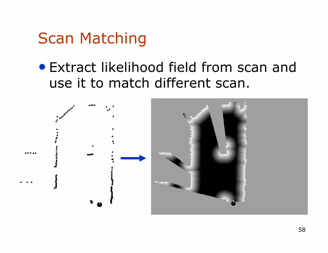
Scan Matching
• Extract likelihood field from scan and use it to match different scan.
61
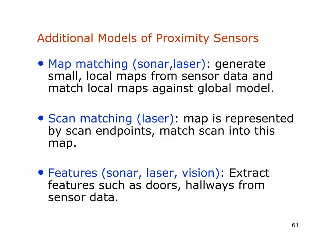
Additional Models of Proximity Sensors
• Map matching (sonar,laser): generate small, local maps from sensor data and match local maps against global model.
• Scan matching (laser): map is represented by scan endpoints, match scan into this map.
• Features (sonar, laser, vision): Extract features such as doors, hallways from sensor data.

62
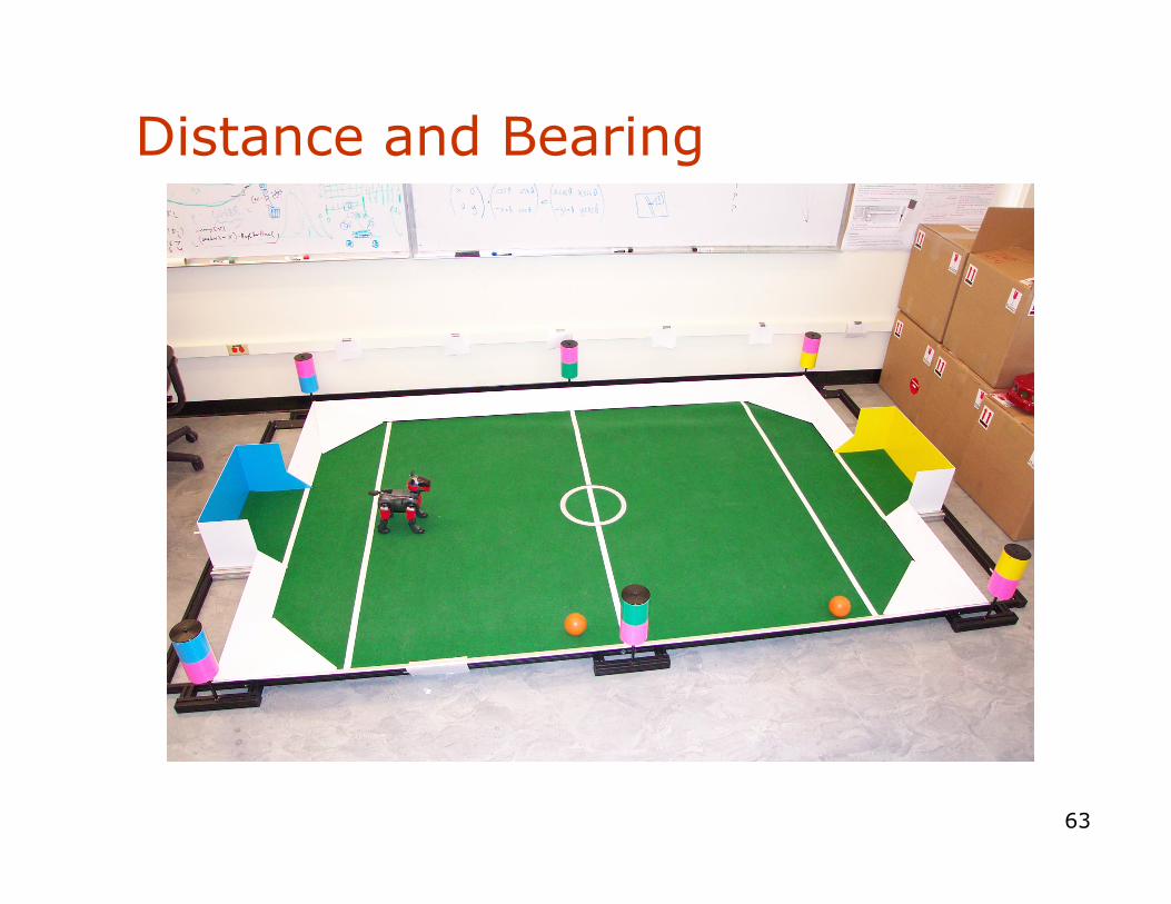
Landmarks
• Active beacons (e.g., radio, GPS) • Passive (e.g., visual, retro-reflective) • Standard approach is triangulation
• Sensor provides • distance, or • bearing, or • distance and bearing.
63
Distance and Bearing

64
Probabilistic Model
1. Algorithm landmark_detection_model(z,x,m):
2.
3.
4.
5. Return
Computing likelihood of landmark measurement
66
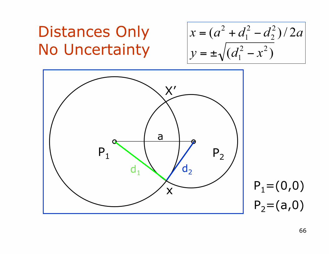
Distances Only No Uncertainty
P1 P2 d1 d2
x
X’
a
P1=(0,0)
P2=(a,0)

67
P1
P2
D1
z1
z2 α
P3
D2 β
z3
D3
Bearings Only No Uncertainty
P1
P2
D1
z1
z2
α
α
Law of cosine
68
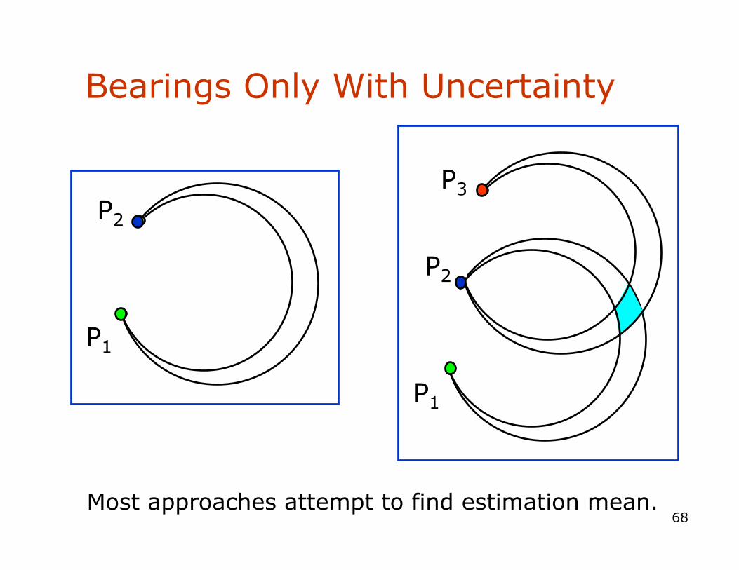
Bearings Only With Uncertainty
P1
P2
P3
P1
P2
Most approaches attempt to find estimation mean.

69
Summary of Sensor Models
• Explicitly modeling uncertainty in sensing is key to robustness.
• In many cases, good models can be found by the following approach:
1. Determine parametric model of noise free measurement. 2. Analyze sources of noise. 3. Add adequate noise to parameters (eventually mix in densities
for noise). 4. Learn (and verify) parameters by fitting model to data. 5. Likelihood of measurement is given by “probabilistically
comparing” the actual with the expected measurement.
• This holds for motion models as well. • It is extremely important to be aware of the underlying
assumptions!


