

Probability Review
Thursday Sep 13
Probability Review• Events and Event spaces• Random variables• Joint probability distributions
• Marginalization, conditioning, chain rule, Bayes Rule, law of total probability, etc.
• Structural properties• Independence, conditional independence
• Mean and Variance• The big picture• Examples

Sample space and Events• Sample Space, result of an experiment
• If you toss a coin twice • Event: a subset of
• First toss is head = {HH,HT}• S: event space, a set of events
• Closed under finite union and complements• Entails other binary operation: union, diff, etc.
• Contains the empty event and

Probability Measure• Defined over (Ss.t.
• P() >= 0 for all in S• P() = 1• If are disjoint, then
• P( U ) = p() + p()• We can deduce other axioms from the above ones
• Ex: P( U ) for non-disjoint eventP( U ) = p() + p() – p(∩

Visualization
• We can go on and define conditional probability, using the above visualization

Conditional ProbabilityP(F|H) = Fraction of worlds in which H is true that also have F true
)(
)()|(
Hp
HFphfp

Rule of total probability
A
B1
B2B3
B4
B5
B6B7
ii BAPBPAp |

From Events to Random Variable• Almost all the semester we will be dealing with RV• Concise way of specifying attributes of outcomes• Modeling students (Grade and Intelligence):
• all possible students• What are events
• Grade_A = all students with grade A• Grade_B = all students with grade B• Intelligence_High = … with high intelligence
• Very cumbersome• We need “functions” that maps from to an
attribute space.• P(G = A) = P({student ϵ G(student) = A})
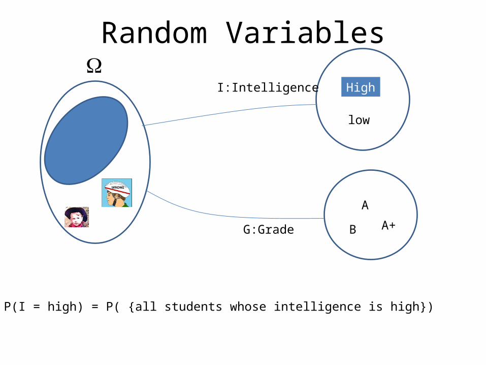
Random Variables
High
low
A
B A+
I:Intelligence
G:Grade
P(I = high) = P( {all students whose intelligence is high})

Discrete Random Variables
• Random variables (RVs) which may take on only a countable number of distinct values– E.g. the total number of tails X you get if you flip
100 coins
• X is a RV with arity k if it can take on exactly one value out of {x1, …, xk}– E.g. the possible values that X can take on are 0, 1,
2, …, 100
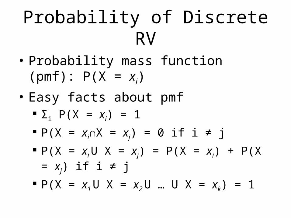
Probability of Discrete RV
• Probability mass function (pmf): P(X = xi)
• Easy facts about pmf Σi P(X = xi) = 1
P(X = xi∩X = xj) = 0 if i ≠ j
P(X = xi U X = xj) = P(X = xi) + P(X = xj) if i ≠ j
P(X = x1 U X = x2 U … U X = xk) = 1

Common Distributions
• Uniform X U[1, …, N] X takes values 1, 2, … N P(X = i) = 1/N E.g. picking balls of different colors from a box
• Binomial X Bin(n, p) X takes values 0, 1, …, n E.g. coin flips
p(X i) n
i
pi(1 p)n i
Continuous Random Variables
• Probability density function (pdf) instead of probability mass function (pmf)
• A pdf is any function f(x) that describes the probability density in terms of the input variable x.
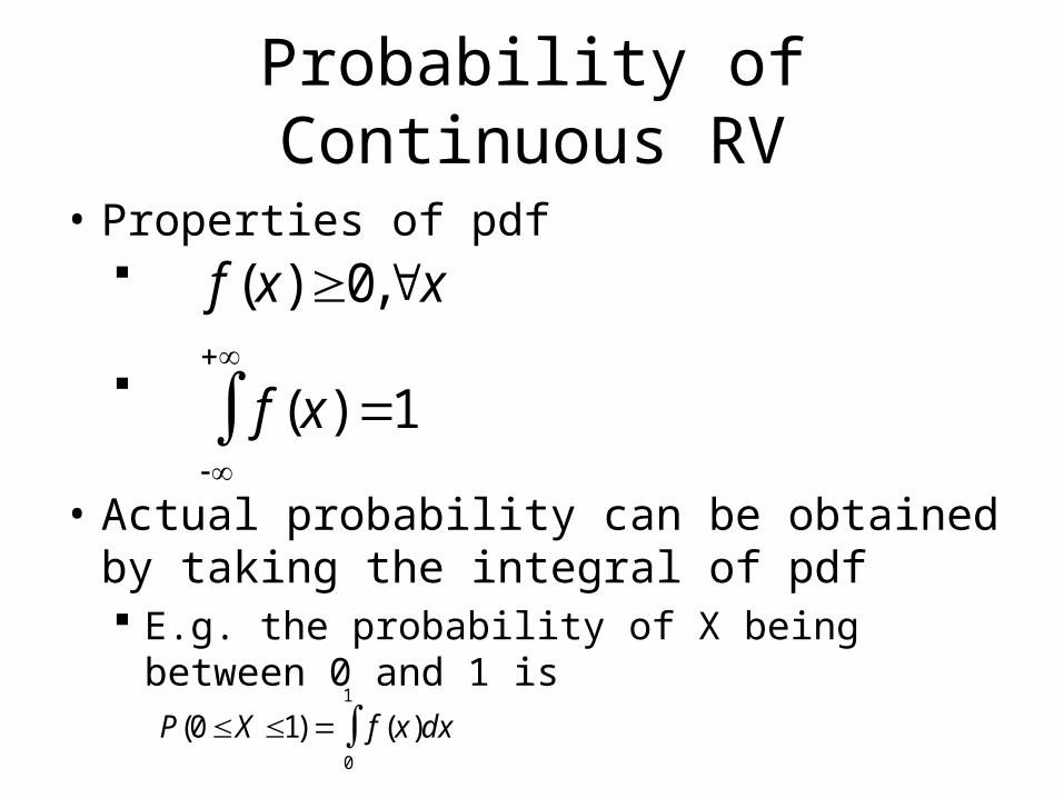
Probability of Continuous RV
• Properties of pdf
• Actual probability can be obtained by taking the integral of pdf E.g. the probability of X being between 0 and 1 is
f (x)0,x
f (x) 1
P(0X 1) f (x)dx0
1

Cumulative Distribution Function
• FX(v) = P(X ≤ v)
• Discrete RVs FX(v) = Σvi P(X = vi)
• Continuous RVs
FX (v) f (x)dx
v
d
dxFx (x) f (x)

Common Distributions
• Normal X N(μ, σ2)
E.g. the height of the entire population
f (x) 1
2exp
(x )2
2 2

Multivariate Normal
• Generalization to higher dimensions of the one-dimensional normal
f r X (x i,..., xd )
1
(2)d / 21/ 2
exp 1
2r x T 1 r
x
.
Covariance matrix
Mean

Probability Review• Events and Event spaces• Random variables• Joint probability distributions
• Marginalization, conditioning, chain rule, Bayes Rule, law of total probability, etc.
• Structural properties• Independence, conditional independence
• Mean and Variance• The big picture• Examples

Joint Probability Distribution• Random variables encodes attributes• Not all possible combination of attributes are equally
likely• Joint probability distributions quantify this
• P( X= x, Y= y) = P(x, y) • Generalizes to N-RVs• •
x y
yYxXP 1,
x y
YX dxdyyxf 1,,

Chain Rule• Always true
• P(x, y, z) = p(x) p(y|x) p(z|x, y) = p(z) p(y|z) p(x|y, z)
=…

Conditional Probability
P X YP X Y
P Y
x yx y
y
)(
),(|
yp
yxpyxP
But we will always write it this way:
events

Marginalization
• We know p(X, Y), what is P(X=x)?• We can use the low of total probability, why?
y
y
yxPyP
yxPxp
|
,
A
B1
B2B3
B4
B5
B6B7
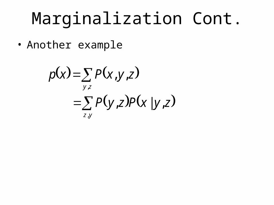
Marginalization Cont.
• Another example
yz
zy
zyxPzyP
zyxPxp
,
,
,|,
,,

Bayes Rule• We know that P(rain) = 0.5
• If we also know that the grass is wet, then how this affects our belief about whether it rains or not?
P rain |wet P(rain)P(wet | rain)
P(wet)
P x | y P(x)P(y | x)
P(y)

Bayes Rule cont.• You can condition on more variables
)|(
),|()|(,|
zyP
zxyPzxPzyxP

Probability Review• Events and Event spaces• Random variables• Joint probability distributions
• Marginalization, conditioning, chain rule, Bayes Rule, law of total probability, etc.
• Structural properties• Independence, conditional independence
• Mean and Variance• The big picture• Examples

Independence• X is independent of Y means that knowing Y
does not change our belief about X.• P(X|Y=y) = P(X) • P(X=x, Y=y) = P(X=x) P(Y=y)• The above should hold for all x, y• It is symmetric and written as X Y

Independence
• X1, …, Xn are independent if and only if
• If X1, …, Xn are independent and identically distributed we say they are iid (or that they are a random sample) and we write
P(X1 A1,...,Xn An ) P X i Ai i1
n
X1, …, Xn ∼ P

CI: Conditional Independence• RV are rarely independent but we can still
leverage local structural properties like Conditional Independence.
• X Y | Z if once Z is observed, knowing the value of Y does not change our belief about X• P(rain sprinkler’s on | cloudy)• P(rain sprinkler’s on | wet grass)

Conditional Independence
• P(X=x | Z=z, Y=y) = P(X=x | Z=z) • P(Y=y | Z=z, X=x) = P(Y=y | Z=z) • P(X=x, Y=y | Z=z) = P(X=x| Z=z) P(Y=y| Z=z)
We call these factors : very useful concept !!

Probability Review• Events and Event spaces• Random variables• Joint probability distributions
• Marginalization, conditioning, chain rule, Bayes Rule, law of total probability, etc.
• Structural properties• Independence, conditional independence
• Mean and Variance• The big picture• Examples
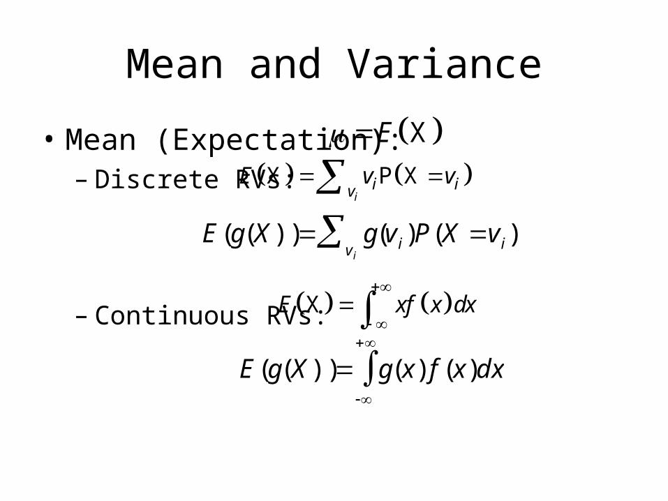
Mean and Variance
• Mean (Expectation): – Discrete RVs:
– Continuous RVs:
XE X P X
ii iv
E v v
XE xf x dx
E(g(X)) g(v i)P(X v i)vi
E(g(X)) g(x) f (x)dx

Mean and Variance• Variance:
– Discrete RVs:
– Continuous RVs:
• Covariance:
• Covariance:
2X P X
ii iv
V v v 2XV x f x dx
Var (X) E((X )2)Var (X) E(X 2) 2
Cov(X,Y ) E((X x )(Y y )) E(XY ) xy

Mean and Variance
• Correlation:
(X,Y ) Cov(X,Y ) / x y
1(X,Y )1

Properties
• Mean– – – If X and Y are independent,
• Variance– – If X and Y are independent,
X Y X YE E E X XE a aE
XY X YE E E
2X XV a b a V
X Y (X) (Y)V V V

Some more properties
• The conditional expectation of Y given X when the value of X = x is:
• The Law of Total Expectation or Law of Iterated Expectation:
dyxypyxXYE )|(*|
dxxpxXYEXYEEYE X )()|()|()(

Some more properties
• The law of Total Variance:
Var (Y ) Var E(Y | X) E Var (Y | X)

Probability Review• Events and Event spaces• Random variables• Joint probability distributions
• Marginalization, conditioning, chain rule, Bayes Rule, law of total probability, etc.
• Structural properties• Independence, conditional independence
• Mean and Variance• The big picture• Examples

The Big Picture
Model Data
Probability
Estimation/learning
Statistical Inference
• Given observations from a model– What (conditional) independence assumptions
hold? • Structure learning
– If you know the family of the model (ex, multinomial), What are the value of the parameters: MLE, Bayesian estimation.
• Parameter learning

Probability Review• Events and Event spaces• Random variables• Joint probability distributions
• Marginalization, conditioning, chain rule, Bayes Rule, law of total probability, etc.
• Structural properties• Independence, conditional independence
• Mean and Variance• The big picture• Examples

Monty Hall Problem
• You're given the choice of three doors: Behind one door is a car; behind the others, goats.
• You pick a door, say No. 1• The host, who knows what's behind the doors, opens
another door, say No. 3, which has a goat.• Do you want to pick door No. 2 instead?
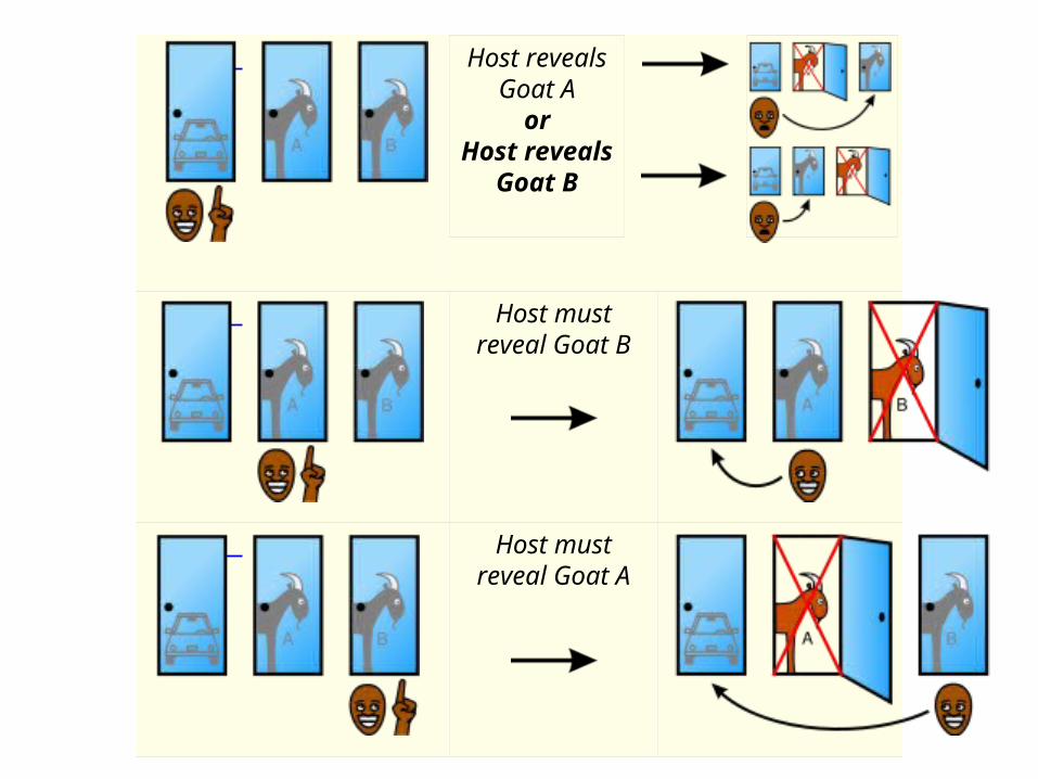
Host mustreveal Goat B
Host mustreveal Goat A
Host revealsGoat A
orHost reveals
Goat B

Monty Hall Problem: Bayes Rule
• : the car is behind door i, i = 1, 2, 3• • : the host opens door j after you pick door i
•
iC
ijH 1 3iP C
0
0
1 2
1 ,
ij k
i j
j kP H C
i k
i k j k

Monty Hall Problem: Bayes Rule cont.• WLOG, i=1, j=3
•
•
13 1 11 13
13
P H C P CP C H
P H
13 1 11 1 1
2 3 6P H C P C

•
•
Monty Hall Problem: Bayes Rule cont.
13 13 1 13 2 13 3
13 1 1 13 2 2
, , ,
1 11
6 31
2
P H P H C P H C P H C
P H C P C P H C P C
1 131 6 1
1 2 3P C H
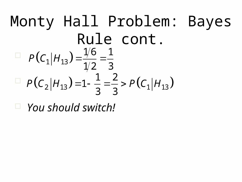
Monty Hall Problem: Bayes Rule cont.
1 131 6 1
1 2 3P C H
You should switch!
2 13 1 131 2
13 3
P C H P C H

Information Theory• P(X) encodes our uncertainty about X
• Some variables are more uncertain that others
• How can we quantify this intuition?• Entropy: average number of bits required to encode X
P(X) P(Y)
X Y
xxP xPxP
xPxP
xpEXH )(log
1log
1log

Information Theory cont.• Entropy: average number of bits required to encode X
• We can define conditional entropy similarly
• i.e. once Y is known, we only need H(X,Y) – H(Y) bits• We can also define chain rule for entropies (not surprising)
YHYXHyxp
EYXH PPP
,
|
1log|
YXZHXYHXHZYXH PPPP ,||,,
xxP xPxP
xPxP
xpEXH )(log
1log
1log

Mutual Information: MI• Remember independence?
• If XY then knowing Y won’t change our belief about X• Mutual information can help quantify this! (not the only
way though)• MI:
• “The amount of uncertainty in X which is removed by knowing Y”
• Symmetric• I(X;Y) = 0 iff, X and Y are independent!
YXHXHYXI PPP |;
y x ypxp
yxpyxpYXI
)()(
),(log),();(

Chi Square Test for Independence(Example)
Republican Democrat Independent Total
Male 200 150 50 400
Female 250 300 50 600
Total 450 450 100 1000
• State the hypothesesH0: Gender and voting preferences are independent.
Ha: Gender and voting preferences are not independent
• Choose significance level Say, 0.05

Chi Square Test for Independence
• Analyze sample data• Degrees of freedom =
|g|-1 * |v|-1 = (2-1) * (3-1) = 2• Expected frequency count =
Eg,v = (ng * nv) / n
Em,r = (400 * 450) / 1000 = 180000/1000 = 180Em,d= (400 * 450) / 1000 = 180000/1000 = 180Em,i = (400 * 100) / 1000 = 40000/1000 = 40Ef,r = (600 * 450) / 1000 = 270000/1000 = 270Ef,d = (600 * 450) / 1000 = 270000/1000 = 270Ef,i = (600 * 100) / 1000 = 60000/1000 = 60
Republican Democrat Independent Total
Male 200 150 50 400
Female 250 300 50 600
Total 450 450 100 1000

Chi Square Test for Independence
• Chi-square test statistic
• Χ2 = (200 - 180)2/180 + (150 - 180)2/180 + (50 - 40)2/40 + (250 - 270)2/270 + (300 - 270)2/270 + (50 - 60)2/40
• Χ2 = 400/180 + 900/180 + 100/40 + 400/270 + 900/270 +100/60
• Χ2 = 2.22 + 5.00 + 2.50 + 1.48 + 3.33 + 1.67 = 16.2
vg
vgvg
E
EOX
,
2,,2 )(
Republican Democrat Independent Total
Male 200 150 50 400
Female 250 300 50 600
Total 450 450 100 1000

Chi Square Test for Independence
• P-value– Probability of observing a sample statistic as
extreme as the test statistic– P(X2 ≥ 16.2) = 0.0003
• Since P-value (0.0003) is less than the significance level (0.05), we cannot accept the null hypothesis
• There is a relationship between gender and voting preference

Acknowledgment
• Carlos Guestrin recitation slides: http://www.cs.cmu.edu/~guestrin/Class/10708/recitations/r1/Probability_and_Statistics_Review.ppt
• Andrew Moore Tutorial: http://www.autonlab.org/tutorials/prob.html
• Monty hall problem:http://en.wikipedia.org/wiki/Monty_Hall_problem
• http://www.cs.cmu.edu/~guestrin/Class/10701-F07/recitation_schedule.html• Chi-square test for independence
http://stattrek.com/chi-square-test/independence.aspx


