Probing causal mechanisms and
strengthening causal inference by
means of mixture mediation modeling
SESSION 3.5: Modeling Treatment and Causal Effects
Modern Modeling Methods Conference, Storrs, CT, May 20-21, 2014
Emil Coman1, Judith Fifield1, Suzanne Suggs2, Deborah Dauser-Forrest1, Martin-Peele Melanie1
1Ethel Donahue TRIPP Center, U. of Connecticut Health Center, 2 Università della Svizzera italiana, Switzerland
The 1st author thanks David Kenny for introducing him to the causal modeling
world through the path analysis backdoor, for his constant mentoring and extensive
generous discussions and advice, and to SEMNET mentors who so generously
shared their time and expertise and taught Latent Variable modeling to many
students of applied statistics across the globe for many years.
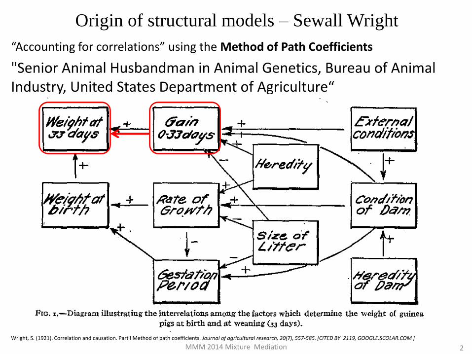
Origin of structural models – Sewall Wright
“Accounting for correlations” using the Method of Path Coefficients
"Senior Animal Husbandman in Animal Genetics, Bureau of Animal Industry, United States Department of Agriculture“
2
Wright, S. (1921). Correlation and causation. Part I Method of path coefficients. Journal of agricultural research, 20(7), 557-585. [CITED BY 2119, GOOGLE.SCOLAR.COM ]
MMM 2014 Mixture Mediation
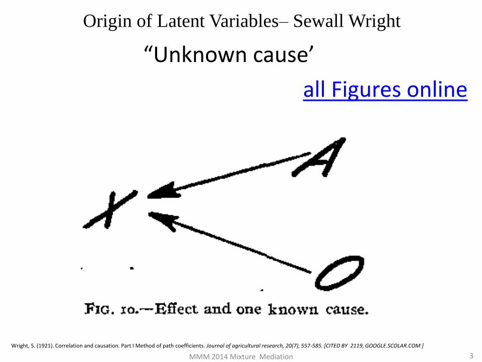
Origin of Latent Variables– Sewall Wright
“Unknown cause’
all Figures online
3
Wright, S. (1921). Correlation and causation. Part I Method of path coefficients. Journal of agricultural research, 20(7), 557-585. [CITED BY 2119, GOOGLE.SCOLAR.COM ]
MMM 2014 Mixture Mediation

Research Questions about the intervention
RQ 1. Is the intervention showing benefits to all
participants?
RQ 2. Do some participants respond better/worse
to the intervention?
RQ 3. Are there mechanisms of change operating
differently in classes of participants?
4 MMM 2014 Mixture Mediation
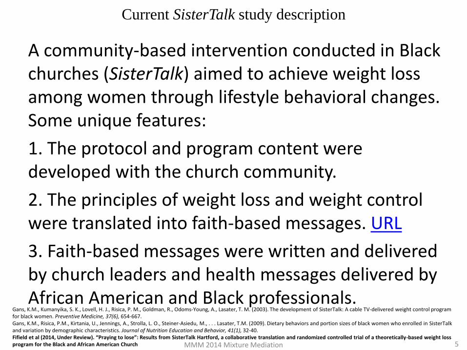
Current SisterTalk study description
MMM 2014 Mixture Mediation 5
A community-based intervention conducted in Black churches (SisterTalk) aimed to achieve weight loss among women through lifestyle behavioral changes. Some unique features:
1. The protocol and program content were developed with the church community.
2. The principles of weight loss and weight control were translated into faith-based messages. URL
3. Faith-based messages were written and delivered by church leaders and health messages delivered by African American and Black professionals.
Gans, K.M., Kumanyika, S. K., Lovell, H. J., Risica, P. M., Goldman, R., Odoms-Young, A., Lasater, T. M. (2003). The development of SisterTalk: A cable TV-delivered weight control program for black women. Preventive Medicine, 37(6), 654-667. Gans, K.M., Risica, P.M., Kirtania, U., Jennings, A., Strolla, L. O., Steiner-Asiedu, M., . . . Lasater, T.M. (2009). Dietary behaviors and portion sizes of black women who enrolled in SisterTalk and variation by demographic characteristics. Journal of Nutrition Education and Behavior, 41(1), 32-40. Fifield et al (2014, Under Review). “Praying to lose”: Results from SisterTalk Hartford, a collaborative translation and randomized controlled trial of a theoretically-based weight loss program for the Black and African American Church
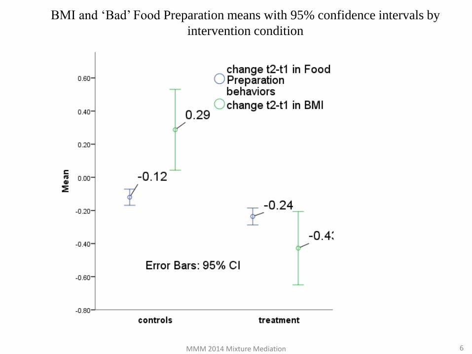
BMI and ‘Bad’ Food Preparation means with 95% confidence intervals by
intervention condition
MMM 2014 Mixture Mediation 6
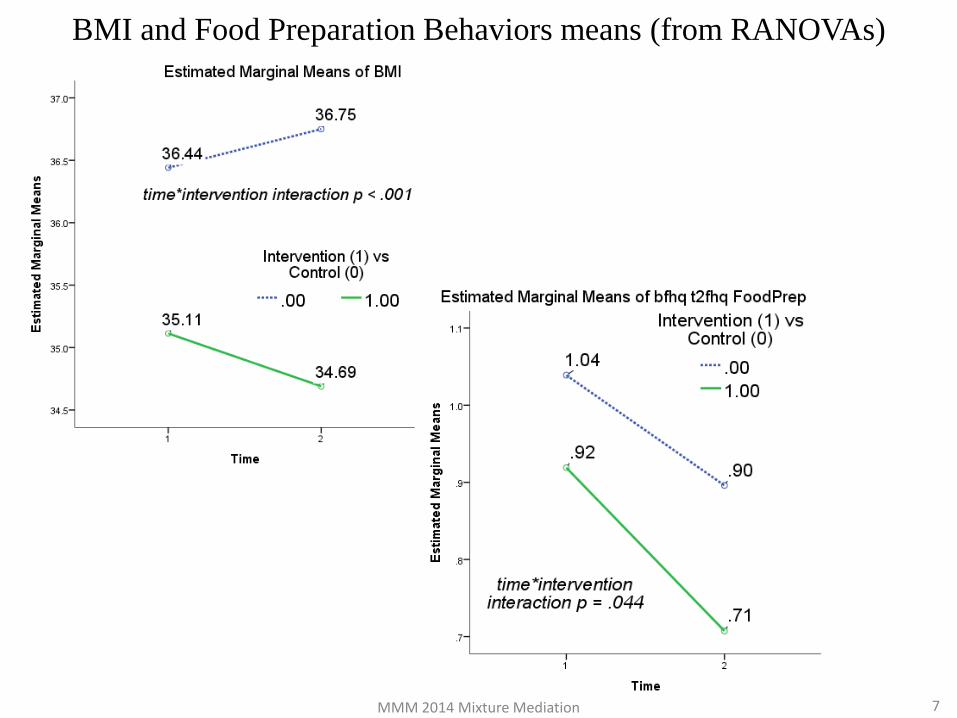
BMI and Food Preparation Behaviors means (from RANOVAs)
MMM 2014 Mixture Mediation 7
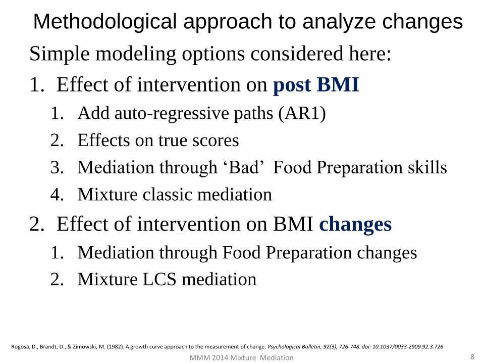
Methodological approach to analyze changes
Simple modeling options considered here:
1. Effect of intervention on post BMI
1. Add auto-regressive paths (AR1)
2. Effects on true scores
3. Mediation through ‘Bad’ Food Preparation skills
4. Mixture classic mediation
2. Effect of intervention on BMI changes
1. Mediation through Food Preparation changes
2. Mixture LCS mediation
8
Rogosa, D., Brandt, D., & Zimowski, M. (1982). A growth curve approach to the measurement of change. Psychological Bulletin, 92(3), 726-748. doi: 10.1037/0033-2909.92.3.726
MMM 2014 Mixture Mediation
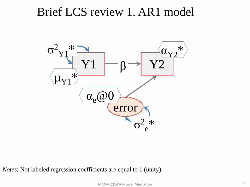
Brief LCS review 1. AR1 model
Notes: Not labeled regression coefficients are equal to 1 (unity).
Y2 Y1
error
µY1*
αY2*
αe@0
β
9
σ2e*
σ2Y1*
MMM 2014 Mixture Mediation
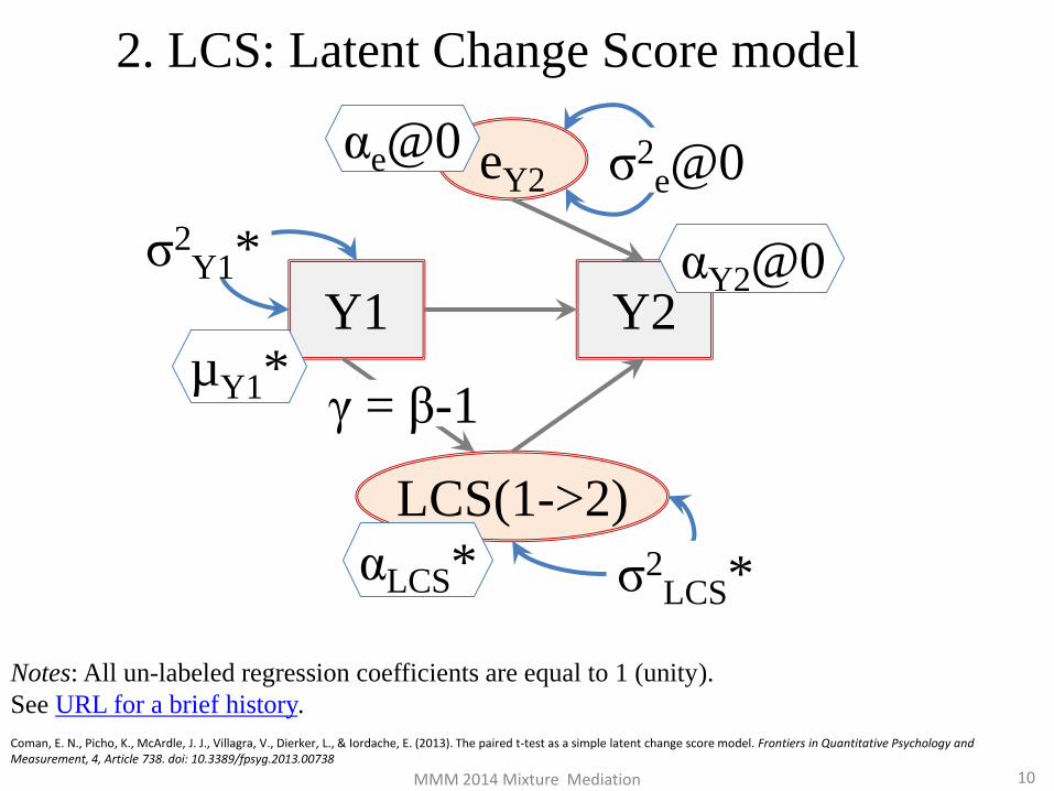
2. LCS: Latent Change Score model
Notes: All un-labeled regression coefficients are equal to 1 (unity).
See URL for a brief history.
Y2 Y1
LCS(1->2)
µY1*
αY2@0
αLCS*
eY2 αe@0
γ = β-1
10
σ2Y1*
σ2e@0
σ2LCS*
Coman, E. N., Picho, K., McArdle, J. J., Villagra, V., Dierker, L., & Iordache, E. (2013). The paired t-test as a simple latent change score model. Frontiers in Quantitative Psychology and Measurement, 4, Article 738. doi: 10.3389/fpsyg.2013.00738
MMM 2014 Mixture Mediation
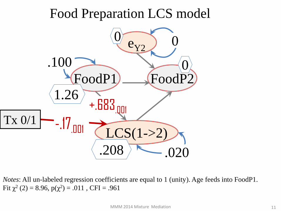
Food Preparation LCS model
Notes: All un-labeled regression coefficients are equal to 1 (unity). Age feeds into FoodP1.
Fit χ2 (2) = 8.96, p(χ2) = .011 , CFI = .961
FoodP2 FoodP1
LCS(1->2)
1.26
0
.208
eY2 0
+.683.001
11
.100
0
.020
Tx 0/1 -.17.001
MMM 2014 Mixture Mediation

BMI LCS model
Notes: All un-labeled regression coefficients are equal to 1 (unity). Age feeds into BMI1.
Fit χ2 (2) = 4.93, p(χ2) = .085 , CFI = .996; residual LCS variance < 0 though.
BMI2 BMI1
LCS(1->2)
41.2
0
0
eY2 0
+1.00.001
12
55.8
0
-4.5
Coman, E. N., Picho, K., McArdle, J. J., Villagra, V., Dierker, L., & Iordache, E. (2013). The paired t-test as a simple latent change score model. Frontiers in Quantitative Psychology and Measurement, 4, Article 738. doi: 10.3389/fpsyg.2013.00738
Tx 0/1 -.75.001
MMM 2014 Mixture Mediation
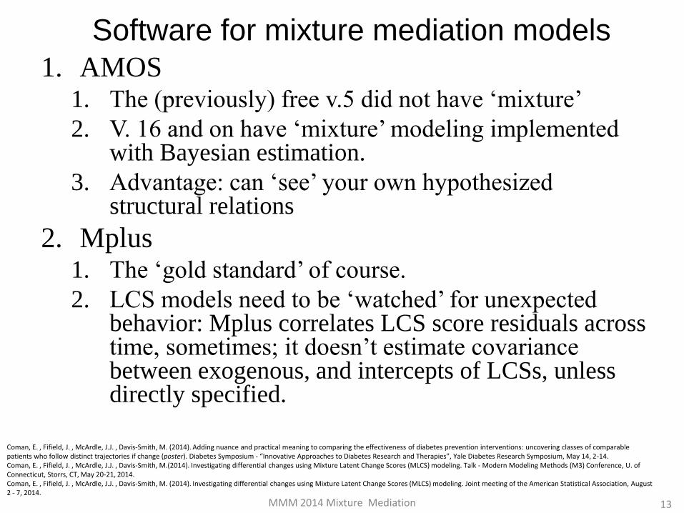
Software for mixture mediation models
1. AMOS 1. The (previously) free v.5 did not have ‘mixture’
2. V. 16 and on have ‘mixture’ modeling implemented with Bayesian estimation.
3. Advantage: can ‘see’ your own hypothesized structural relations
2. Mplus 1. The ‘gold standard’ of course.
2. LCS models need to be ‘watched’ for unexpected behavior: Mplus correlates LCS score residuals across time, sometimes; it doesn’t estimate covariance between exogenous, and intercepts of LCSs, unless directly specified.
13
Coman, E. , Fifield, J. , McArdle, J.J. , Davis-Smith, M. (2014). Adding nuance and practical meaning to comparing the effectiveness of diabetes prevention interventions: uncovering classes of comparable patients who follow distinct trajectories if change (poster). Diabetes Symposium - “Innovative Approaches to Diabetes Research and Therapies”, Yale Diabetes Research Symposium, May 14, 2-14. Coman, E. , Fifield, J. , McArdle, J.J. , Davis-Smith, M.(2014). Investigating differential changes using Mixture Latent Change Scores (MLCS) modeling. Talk - Modern Modeling Methods (M3) Conference, U. of Connecticut, Storrs, CT, May 20-21, 2014. Coman, E. , Fifield, J. , McArdle, J.J. , Davis-Smith, M. (2014). Investigating differential changes using Mixture Latent Change Scores (MLCS) modeling. Joint meeting of the American Statistical Association, August 2 - 7, 2014.
MMM 2014 Mixture Mediation
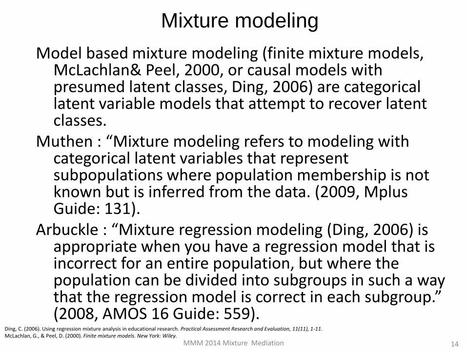
Mixture modeling
14
Ding, C. (2006). Using regression mixture analysis in educational research. Practical Assessment Research and Evaluation, 11(11), 1-11. McLachlan, G., & Peel, D. (2000). Finite mixture models. New York: Wiley.
Model based mixture modeling (finite mixture models, McLachlan& Peel, 2000, or causal models with presumed latent classes, Ding, 2006) are categorical latent variable models that attempt to recover latent classes.
Muthen : “Mixture modeling refers to modeling with categorical latent variables that represent subpopulations where population membership is not known but is inferred from the data. (2009, Mplus Guide: 131).
Arbuckle : “Mixture regression modeling (Ding, 2006) is appropriate when you have a regression model that is incorrect for an entire population, but where the population can be divided into subgroups in such a way that the regression model is correct in each subgroup.” (2008, AMOS 16 Guide: 559).
MMM 2014 Mixture Mediation
Mixture modeling
(MM) – Jeff Harring
15
Harring, J. R. (December 4, 5 & 6, 2013). Introduction to Finite Mixture Models. Details: http://www.cilvr.umd.edu/Workshops/CILVRworkshoppageFMM2013.html College Park, Maryland. Pearson, K. (1894). Contributions to the mathematical theory of evolution. Philosophical Transactions of the Royal Society of London. A, 185, 71-110.
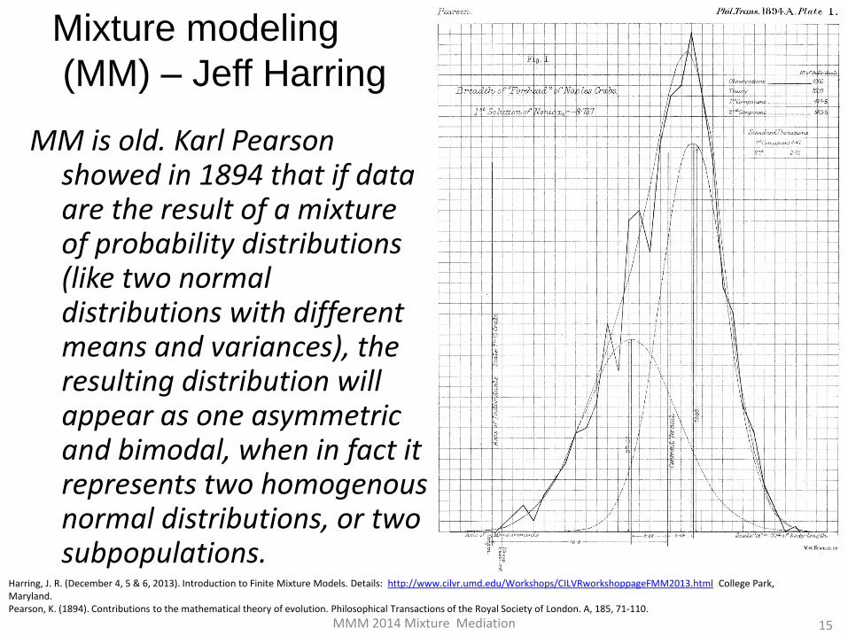
MM is old. Karl Pearson showed in 1894 that if data are the result of a mixture of probability distributions (like two normal distributions with different means and variances), the resulting distribution will appear as one asymmetric and bimodal, when in fact it represents two homogenous normal distributions, or two subpopulations.
MMM 2014 Mixture Mediation
Mixture modeling (MM) – Jeff Harring
16 Harring, J. R. (December 4, 5 & 6, 2013). Introduction to Finite Mixture Models. Details: http://www.cilvr.umd.edu/Workshops/CILVRworkshoppageFMM2013.html. College Park, Maryland.
The general mixture specification assumes a composite (mixed)
distribution as the sum of K classes pdf’s (probability density
functions) distributions, each with class-specific parameters θk, and
weights or mixing proportions φi, which specify in fact the class
proportions.
The likelihood for one patient’s observations is then obtained as the
probability of his/her data as a function of the parameters, and then a
global likelihood function L is calculated as the product of individual
patients’ likelihoods.
Using Maximum Likelihood (ML) or Bayesian estimation, one can then
obtain the parameter values that maximize the loglikelihood L.
MM software use in practice is an Expectation-Maximization (EM)
algorithm, which acts as an optimizer (not estimator) by generating
starting values for the parameters θk and then, given posterior
probabilities for φik, obtains new estimates for φik and θk, and
continues in such steps until the change in the likelihood from
successive iterations is sufficiently small. (Harring, 2013).
MMM 2014 Mixture Mediation
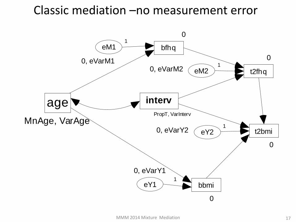
Classic mediation –no measurement error
0
bfhq
0
t2fhq0, eVarM2 eM2
MnAge, VarAge
age
0, eVarM1
eM1
0
bbmi
0
t2bmi0, eVarY2 eY2
0, eVarY1
eY1
1
1
1
1
PropT, VarInterv
interv
MMM 2014 Mixture Mediation 17
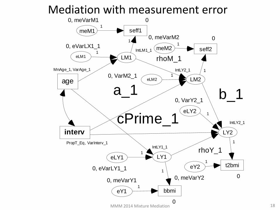
Mediation with measurement error 0
seff1
0
seff2
0, meVarM2
meM2
MnAge_1, VarAge_1
age
0, meVarM1
meM1
0
bbmi
0
t2bmi
0, meVarY2
eY2
0, meVarY1
eY1
IntLY2_1
LY2
IntLY1_1
LY1
IntLM1_1
LM1
IntLY2_1
LM2
1
1
0, eVarLX1_1
eLM1
0, VarM2_1eLM2
0, VarY2_1
eLY2
0, eVarLY1_1
eLY1
1
1
1
1
1
1
rhoM_1
rhoY_1
1
1
1
1
PropT_Eq, VarInterv_1
interv
a_1
cPrime_1
b_1
MMM 2014 Mixture Mediation 18
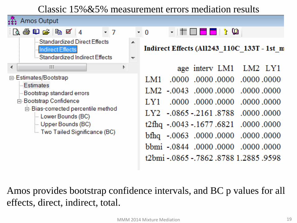
Classic 15%&5% measurement errors mediation results
Amos provides bootstrap confidence intervals, and BC p values for all
effects, direct, indirect, total.
MMM 2014 Mixture Mediation 19
FoodPrep2
Tx 0/1
BMI2
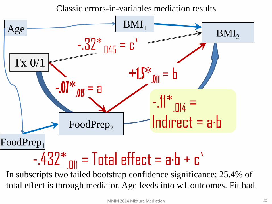
Classic errors-in-variables mediation results
-.11*.014 =
Indirect = a·b
In subscripts two tailed bootstrap confidence significance; 25.4% of
total effect is through mediator. Age feeds into w1 outcomes. Fit bad.
-.07*.015 = a
-.32*.045 = c’
+1.5*.011 = b
-.432*.011 = Total effect = a·b + c’
MMM 2014 Mixture Mediation 20
BMI1
FoodPrep1
Age
FoodPrep2
Tx 0/1
BMI2
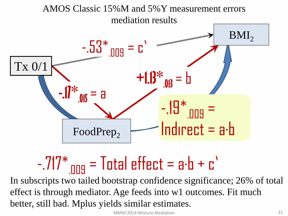
AMOS Classic 15%M and 5%Y measurement errors
mediation results
-.19*.009 =
Indirect = a·b
In subscripts two tailed bootstrap confidence significance; 26% of total
effect is through mediator. Age feeds into w1 outcomes. Fit much
better, still bad. Mplus yields similar estimates.
-.17*.015 = a
-.53*.009 = c’
+1.13*.013 = b
-.717*.009 = Total effect = a·b + c’
MMM 2014 Mixture Mediation 21
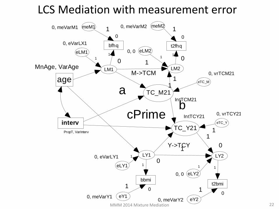
LCS Mediation with measurement error
IntTCM21
TC_M21
0
bfhq
0
t2fhq
0, meVarM2 meM2
0, vrTCM21
eTC_M
MnAge, VarAge
age
0, meVarM1 meM1
IntTCY21
TC_Y21
0
bbmi
0
t2bmi
0, meVarY2 eY2
0, vrTCY21
eTC_Y
0, meVarY1 eY1
1
1
0
LY20
LY1
0
LM1
0
LM2
Y->TCY
1
1M->TCM
11
0, eVarLX1
eLM1 0, 0 eLM2
0, 0 eLY2
0, eVarLY1
eLY1
1 1
1
1
1 1
1
1
11
11
PropT, VarInterv
interv
a
bcPrime
MMM 2014 Mixture Mediation 22
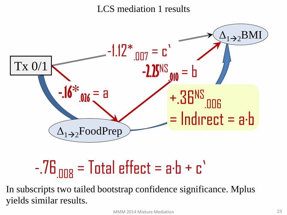
Δ12FoodPrep
Tx 0/1
Δ12BMI
LCS mediation 1 results
+.36NS.006
= Indirect = a·b
In subscripts two tailed bootstrap confidence significance. Mplus
yields similar results.
-.16*.026 = a
-1.12*.007 = c’
-2.25NS.010 = b
-.76.008 = Total effect = a·b + c’
MMM 2014 Mixture Mediation 23
FAT intake
behaviors2
0/1 BMI2
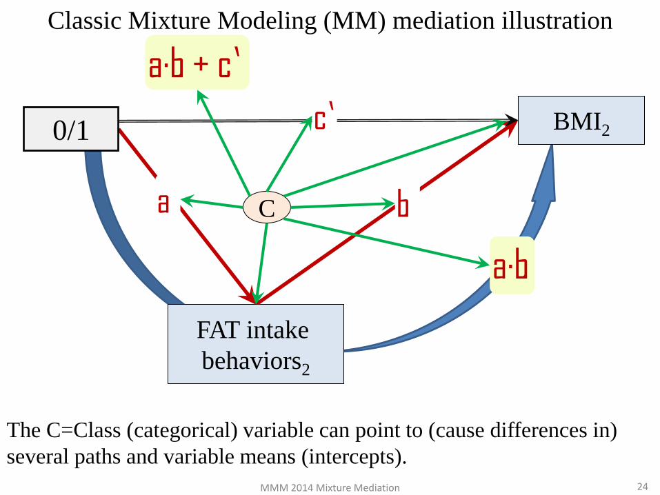
Classic Mixture Modeling (MM) mediation illustration
a·b
The C=Class (categorical) variable can point to (cause differences in)
several paths and variable means (intercepts).
c’ a·b + c’
b a C
MMM 2014 Mixture Mediation 24
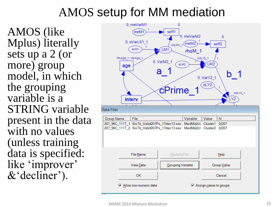
AMOS setup for MM mediation
25
AMOS (like Mplus) literally sets up a 2 (or more) group model, in which the grouping variable is a STRING variable present in the data with no values (unless training data is specified: like ‘improver’ &‘decliner’).
MMM 2014 Mixture Mediation
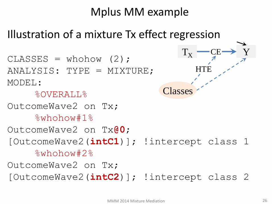
Mplus MM example
26
Illustration of a mixture Tx effect regression
CLASSES = whohow (2);
ANALYSIS: TYPE = MIXTURE;
MODEL:
%OVERALL%
OutcomeWave2 on Tx;
%whohow#1%
OutcomeWave2 on Tx@0;
[OutcomeWave2(intC1)]; !intercept class 1
%whohow#2%
OutcomeWave2 on Tx;
[OutcomeWave2(intC2)]; !intercept class 2
YTX CE
Classes
HTE
MMM 2014 Mixture Mediation
FoodPrep2
0/1
BMI2
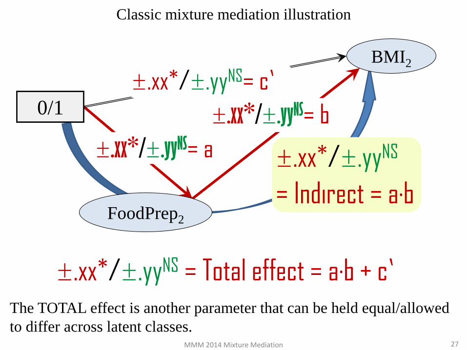
Classic mixture mediation illustration
±.xx*/±.yyNS
= Indirect = a·b
The TOTAL effect is another parameter that can be held equal/allowed
to differ across latent classes.
±.xx*/±.yyNS= a
±.xx*/±.yyNS= c’
±.xx*/±.yyNS= b
±.xx*/±.yyNS = Total effect = a·b + c’
27 MMM 2014 Mixture Mediation
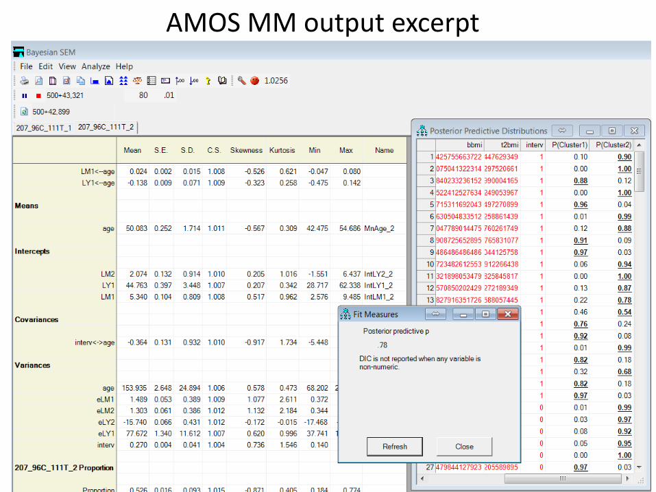
AMOS MM output excerpt
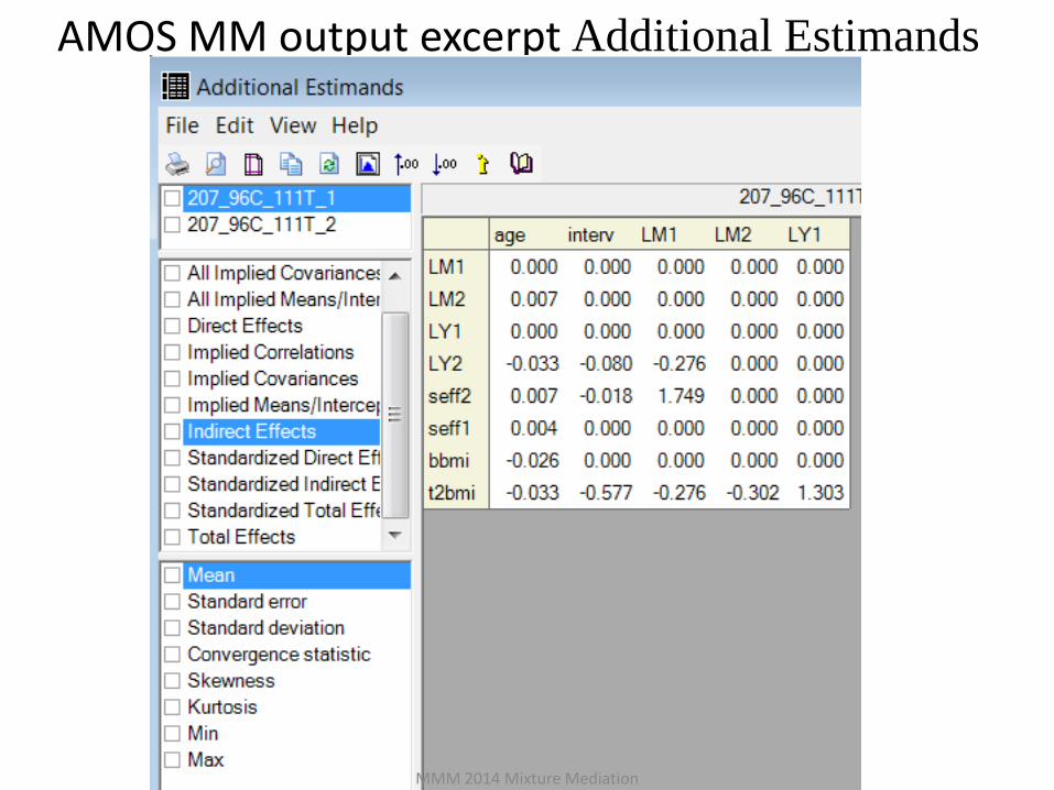
AMOS MM output excerpt Additional Estimands
MMM 2014 Mixture Mediation
FoodPrep2
Tx 0/1
BMI2
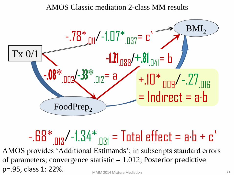
AMOS Classic mediation 2-class MM results
+.10*.009/-.27.016
= Indirect = a·b
AMOS provides ‘Additional Estimands’; in subscripts standard errors
of parameters; convergence statistic = 1.012; Posterior predictive p=.95, class 1: 22%.
-.08*.002/-.33*.012= a
-.78*.011/-1.07*.037= c’
-1.21.088/+.81.041= b
-.68*.013/-1.34*.031 = Total effect = a·b + c’
MMM 2014 Mixture Mediation 30
Classic Mediation Mixture modeling results
31
The classic mediation MM seem to extract
I. 2 similar classes in terms of the total effects, but
II. distinct in indirect effects: leading to decline and
improvement, respectively (AMOS results).
III. The Mplus results suggest no significant indirect
effects in either class.
MMM 2014 Mixture Mediation
Δ12FoodPrep
0/1
Δ12BMI
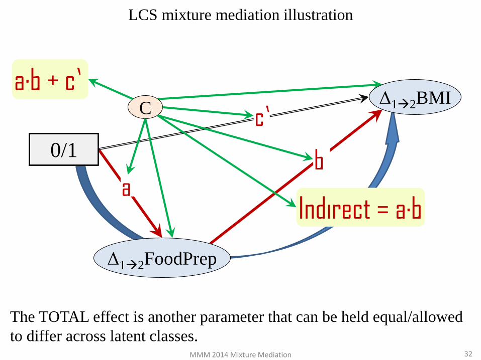
LCS mixture mediation illustration
Indirect = a·b
The TOTAL effect is another parameter that can be held equal/allowed
to differ across latent classes.
a
c’
b
C
MMM 2014 Mixture Mediation 32
a·b + c’
Δ12FoodPrep
0/1
Δ12BMI
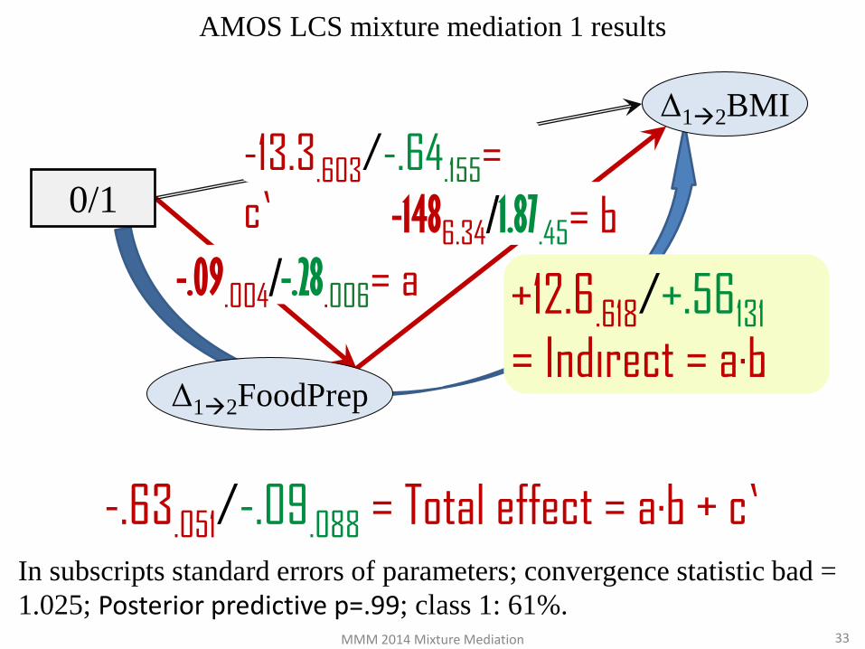
AMOS LCS mixture mediation 1 results
+12.6.618/+.56131
= Indirect = a·b
In subscripts standard errors of parameters; convergence statistic bad =
1.025; Posterior predictive p=.99; class 1: 61%.
-.09.004/-.28.006= a
-13.3.603/-.64.155=
c’ -1486.34/1.87.45= b
-.63.051/-.09.088 = Total effect = a·b + c’
MMM 2014 Mixture Mediation 33
LCS Mediation Mixture modeling results
34
The LCS MM yield a different picture in AMOS and
Mplus:
I. significant and non-significant total effects in the 2
classes
II. no direct effect in either class, and
III. only the a leg significant in AMOS in both classes,
or either the a or b leg significant in the Mplus
results.
MMM 2014 Mixture Mediation
Mediation Mixture modeling Conclusions
35
Kenny, D.A. and C.M. Judd, Power anomalies in testing mediation. Psychological Science, 2013: p. 0956797613502676.
While the MM mediation is not aiming directly at uncovering
classes of cases for which specific indirect effects elements
(the a X-to-M, the b M-to-Y, the c X-to-Y, and the c' total
effect) are/not significant, the procedure does reveal such
classes. Specific input conditions can be entered for unique
expected scenarios, like no a path in one class, but no b
path in another, leading to no indirect effect in either.
There are many moving parts in mixture mediation, let alone
dynamic (LCS) mixture mediation models. Substantive
knowledge needs to be fed into expectations about class
parameters, so that meaningful classes can be extracted.
For example, one should not let the optimizing algorithm
search blindly for total effect parameters, but feed in starting
values (in Mplus) like c1=0 & c2>0.
MMM 2014 Mixture Mediation