
1
MANE 4240 & CIVL 4240Introduction to Finite Elements
Prof. Suvranu De
Development of Truss Equations
Reading assignment:
Chapter 3: Sections 3.1-3.9 + Lecture notes
Summary:
• Stiffness matrix of a bar/truss element • Coordinate transformation• Coordinate transformation• Stiffness matrix of a truss element in 2D space•Problems in 2D truss analysis (including multipoint constraints)•3D Truss element
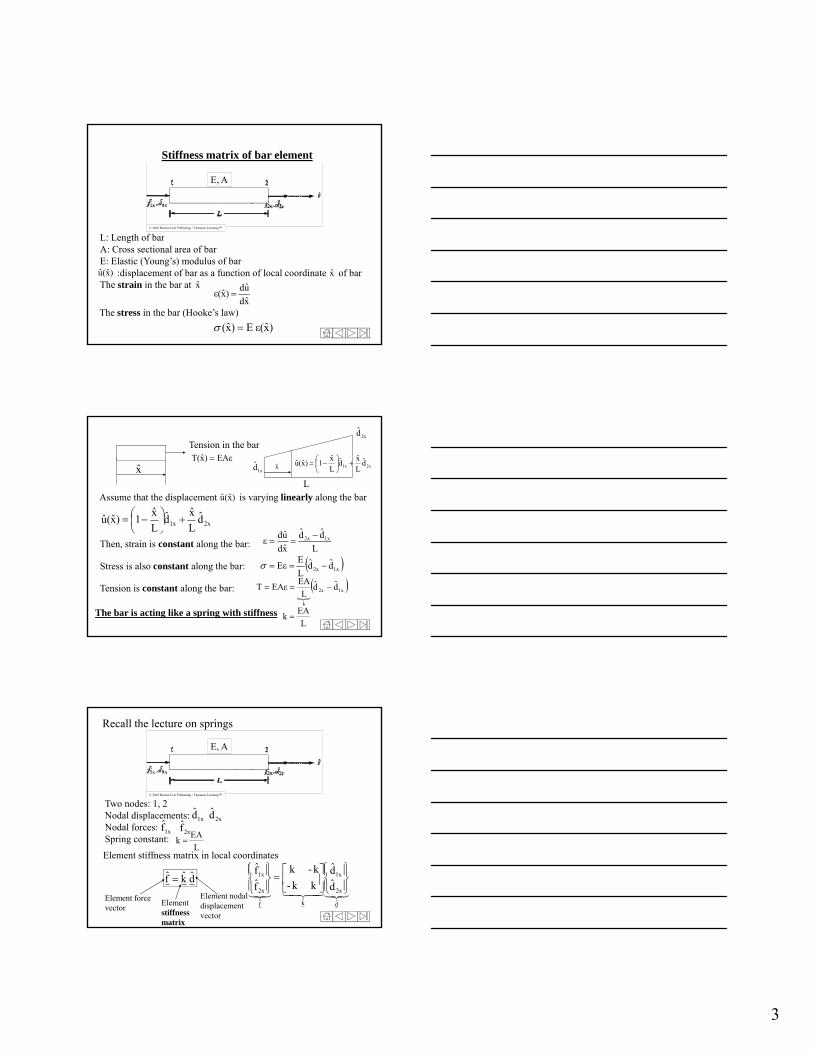
Trusses: Engineering structures that are composed only of two-force members. e.g., bridges, roof supports
Actual trusses: Airy structures composed of slender members (I-beams, channels, angles, bars etc) joined together at their ends by welding, riveted connections or large bolts and pins
Gusset plate
A typical truss structure

2
Ideal trusses:
Assumptions
• Ideal truss members are connected only at their ends.
• Ideal truss members are connected by frictionless pins (no moments)
• The truss structure is loaded only at the pins
• Weights of the members are neglected
A typical truss structureFrictionless pin
These assumptions allow us to idealize each truss member as a two-force member (members loaded only at their extremities by equal opposite and collinear forces)
member in compression
member in tension
Connecting pin
FEM analysis scheme
Step 1: Divide the truss into bar/truss elements connected to each other through special points (“nodes”)
Step 2: Describe the behavior of each bar element (i.e. derive its stiffness matrix and load vector in local AND global coordinate system)system)
Step 3: Describe the behavior of the entire truss by putting together the behavior of each of the bar elements (by assemblingtheir stiffness matrices and load vectors)
Step 4: Apply appropriate boundary conditions and solve
3
L L h f b
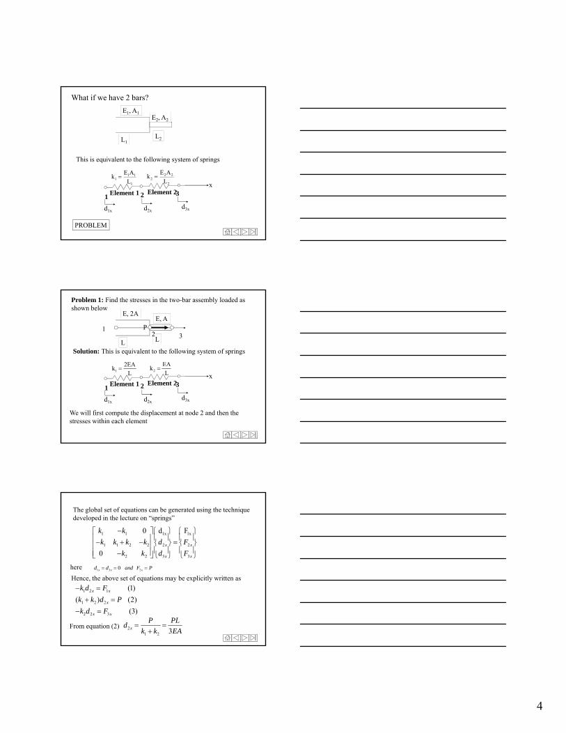
Stiffness matrix of bar element
© 2002 Brooks/Cole Publishing / Thomson Learning™
E, A
L: Length of barA: Cross sectional area of barE: Elastic (Young’s) modulus of bar
:displacement of bar as a function of local coordinate of barThe strain in the bar at x
xd
ud)xε(
x)x(u
The stress in the bar (Hooke’s law)
)xε( E)x(
EAε)xT( Tension in the bar
2x1x dL
xd
L
x1)x(u
x
Assume that the displacement is varying linearly along the bar)x(u
2xd
1xd 2x1x dL
xd
L
x1)x(u
x
L
LL Then, strain is constant along the bar: L
dd
xd
udε 1x2x
Stress is also constant along the bar: 1x2x ddL
EEε
Tension is constant along the bar:
1x2x
k
ddL
EAEAεT
The bar is acting like a spring with stiffnessL
EAk
Recall the lecture on springs
© 2002 Brooks/Cole Publishing / Thomson Learning™
E, A
Two nodes: 1, 2Nodal displacements: 1d 2dNodal displacements:Nodal forces:Spring constant:
1xd 2xd
1xf 2xf
L
EAk
dkf
d
2x
1x
kf
2x
1x
d
d
kk-
k-k
f
f
Element force vector
Element nodal displacement vector
Element stiffness matrix
Element stiffness matrix in local coordinates
4
What if we have 2 bars?
E1, A1E2, A2
L1L2
This is equivalent to the following system of springs
1
111 L
AEk
x
1 2 3Element 1 Element 2
d1x d2xd3x
2
222 L
AEk
PROBLEM
Problem 1: Find the stresses in the two-bar assembly loaded as shown below
E, 2AE, A
L L
2EAk
EAk
Solution: This is equivalent to the following system of springs
12 3
P
1
2EAk
L
x
1 2 3Element 1 Element 2
d1x d2xd3x
2kL
We will first compute the displacement at node 2 and then the stresses within each element
The global set of equations can be generated using the technique developed in the lecture on “springs”
1 1 1x 1x
1 1 2 2 2 2
2 2 3 3
0 d F
0x x
x x
k k
k k k k d F
k k d F
here 1 3 20d d and F P here 1 3 20x x xd d and F P
Hence, the above set of equations may be explicitly written as
1 2 1
1 2 2
2 2 3
(1)
( ) (2)
(3)
x x
x
x x
k d F
k k d P
k d F
From equation (2) 21 2 3x
P PLd
k k EA

5
To calculate the stresses:For element #1 first compute the element strain
(1) 2 1 2
3x x xd d d P
L L EA
and then the stress as(1) (1)
3
PE
A (element in tension)
Similarly, in element # 2
3A
(2) 3 2 2
3x x xd d d P
L L EA
(2) (2)
3
PE
A (element in compression)
© 2002 Brooks/Cole Publishing / Thomson Learning™g g
Inter-element continuity of a two-bar structure
Bars in a truss have various orientations
member in compression
member in tension
Connecting pin

6
xy
θ
1x1x f,d
2x2x f,d
1x1x f,d
1y1y f,d
2y2y f,d
2x2x f,d
x
y
At node 1: At node 2:
1y 1yˆ ˆd , f 0
2y 2yˆ ˆd , f 0
At node 1: At node 2:
1xd
1yd1xdθ
1yd
2xd
2yd2xdθ
2yd
1xf
1yf1xfθ
1yf 0
2xf
2yf2xfθ
2yf 0
In the global coordinate system, the vector of nodal displacements and loads
2y
2x
1y
1x
2y
2x
1y
1x
f
ff
f
f;
d
dd
d
d
Our objective is to obtain a relation of the form
144414dkf
Where k is the 4x4 element stiffness matrix in global coordinate system
The key is to look at the local coordinates
2x
1x
2x
1x
d
d
kk-
k-k
f
f
L
EAk
xy
θ
1x1x f,d
2x2x f,d
x
y
1y 1yˆ ˆd , f 0
2y 2yˆ ˆd , f 0
Rewrite as
2y
2x
1y
1x
2y
2x
1y
1x
d
d
d
d
0000
0k0k-
0000
0k-0k
f
f
f
f
dkf
7
NOTES
1. Assume that there is no stiffness in the local y direction.
2. If you consider the displacement at a point along the local x direction as a vector, then the components of that vector along the
^
global x and y directions are the global x and y displacements.
3. The expanded stiffness matrix in the local coordinates is symmetric and singular.
NOTES5. In local coordinates we have
But or goal is to obtain the following relationship
Hence, need a relationship between and
144414dkf
144414dkf
d dˆand between and f f
2y
2x
1y
1x
2y
2x
1y
1x
d
d
d
d
d
d
dd
d
d
Need to understand how the components of a vector change with coordinate transformation
1xd
1yd1xdθ
1yd
2xd
2yd2xdθ
2yd
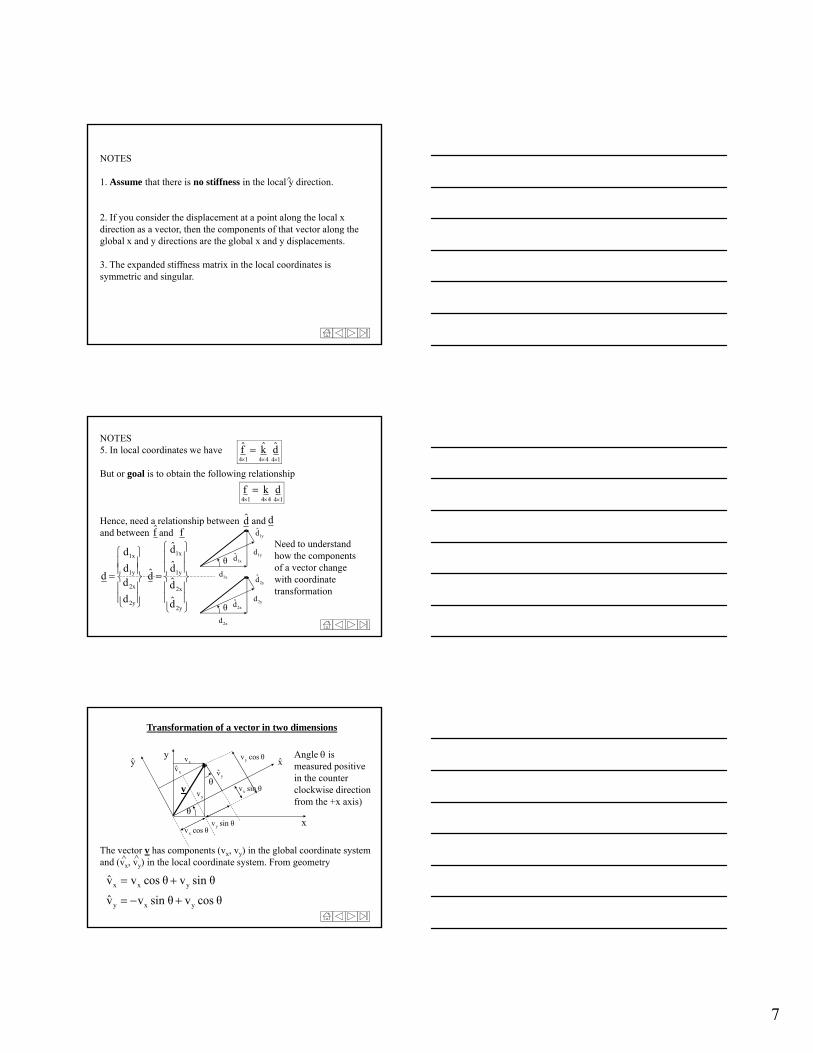
Transformation of a vector in two dimensions
θ
xyyv
y
v
xvxv
yv
θ
yv cos θ
xv sin θ
Angle is measured positive in the counter clockwise direction from the +x axis)
xv cos θxyv sin θ
x x y
y x y
v v cos θ v sin θ
v v sin θ v cos θ
The vector v has components (vx, vy) in the global coordinate system and (vx, vy) in the local coordinate system. From geometry^ ^
8
x x
y y
v vcos θ sin θ
v vsin θ cos θ
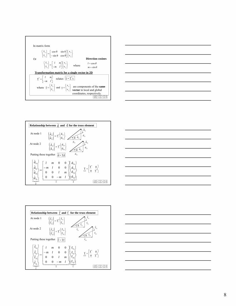
In matrix form
Or
x x
y y
v v
v v
l m
m l
where
sin
cos
m
l
Direction cosines
y y
Transformation matrix for a single vector in 2D
lm
ml*T*v T v
x x
y y
v vv and v
v v
relates
where are components of the same vector in local and global coordinates, respectively.
d dRelationship between and for the truss element
1y
1x*
1y
1x
d
dT
d
dAt node 1
At node 2
2y
2x*
2y
2x
d
dT
d
d1xd
1yd1xdθ
1yd
2yd2xdθ
2yd
Putting these together
d
2y
2x
1y
1x
Td
2y
2x
1y
1x
d
dd
d
00
00
00
00
d
d
d
d
lm
ml
lm
ml
dTd
*
*
44 T0
0TT
2xd
Relationship between and for the truss elementf f
1y
1x*
1y
1x
f
fT
f
fAt node 1
At node 2
2y
2x*
2y
2x
f
fT
f
f 1xf
1yf1xfθ
1yf
2yf2xfθ
2yf
Putting these together
f
2y
2x
1y
1x
Tf
2y
2x
1y
1x
f
ff
f
00
00
00
00
f
f
f
f
lm
ml
lm
ml
fTf
*
*
44 T0
0TT
2xf
9
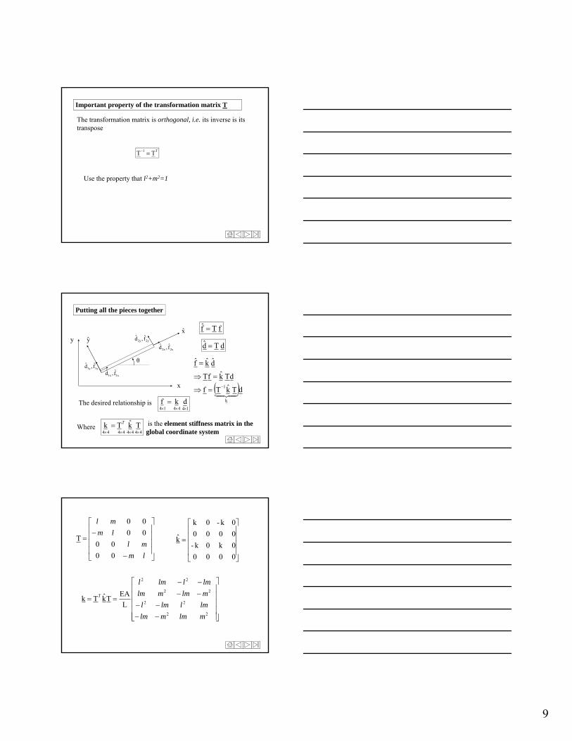
Important property of the transformation matrix T
The transformation matrix is orthogonal, i.e. its inverse is its transpose
TTT 1
Use the property that l2+m2=1
Putting all the pieces together
dkf
xy
θ
ˆˆ
2x2x f,dy
1y1y f,d
2y2y f,d
fTf
dTd
dTkTf
dTkfT
k
1
1x1x f,d
x
The desired relationship is144414
dkf
Where 44444444
TkTk
T is the element stiffness matrix in the global coordinate system
lm
ml
lm
ml
00
00
00
00
T
0000
0k0k-
0000
0k-0k
k
22
22
22
22
L
EATkTk
mlmmlm
lmllml
mlmmlm
lmllml
T

10
Computation of the direction cosines
L
1
2
θ
(x1,y1)
(x2,y2)
L
yym
L
xxl
12
12
sin
cos
What happens if I reverse the node numbers?
L
2
1
θ
(x1,y1)
(x2,y2)
mL
yym
lL
xxl
21
21
sin'
cos'
Question: Does the stiffness matrix change?
© 2002 Brooks/Cole Publishing / Thomson Learning™
Example Bar element for stiffness matrix evaluation
30
60
2
10302
6
inL
inA
psiE
130sin
2
330cos
m
l
230sin m
in
lb
4
1
4
3
4
1
4
34
3
4
3
4
3
4
34
1
4
3
4
1
4
34
3
4
3
4
3
4
3
60
21030k
6
© 2002 Brooks/Cole Publishing / Thomson Learning™
Computation of element strains
d
d
d
d
0101L
1
L
ddε
2x
1y
1x
1x2x
Recall that the element strain is
dT0101L
1
d0101L
1
d 2y

11
d
dL
1
d
00
00
00
00
0101L
1ε
mlml
lm
ml
lm
ml
2y
2x
1y
1x
d
dd
d
L
1mlml
Computation of element stresses stress and tension
dL
Edd
L
EEε 1x2x mlml
Recall that the element stress is
Recall that the element tension is
EAT EAε d
Ll m l m
Recall that the element tension is
Steps in solving a problem
Step 1: Write down the node-element connectivity tablelinking local and global nodes; also form the table of direction cosines (l, m)
Step 2: Write down the stiffness matrix of each element in global coordinate system with global numbering
St 3 A bl th l t tiff t i t f thStep 3: Assemble the element stiffness matrices to form the global stiffness matrix for the entire structure using the node element connectivity table
Step 4: Incorporate appropriate boundary conditions
Step 5: Solve resulting set of reduced equations for the unknowndisplacements
Step 6: Compute the unknown nodal forces

12
Node element connectivity table
ELEMENT Node 1 Node 2
1 1 2
2 2 3
3 3 1
1
2 3
El 1
El 2
El 3
L
1
2
θ
(x1,y1)
(x2,y2)
60 60
60
)1(k
Stiffness matrix of element 1
d1x
d2x
d2xd1x d1y d2y
d1y
d2y
Stiffness matrix of element 2
)2(k
d2x
d3x
d3xd2y d3y
d2y
d3y
d2x
Stiffness matrix of element 3
)3(k
d3x
d1x
d1xd3y d1y
d3y
d1y
d3xThere are 4 degrees of freedom (dof) per element (2 per node)
Global stiffness matrix
K
d2x
d3xd2x
d1x
d1x
d2y
d1y
d1y d2y d3y
)2(k
)1(k
66
d3x
d3y
How do you incorporate boundary conditions?
)3(k
13
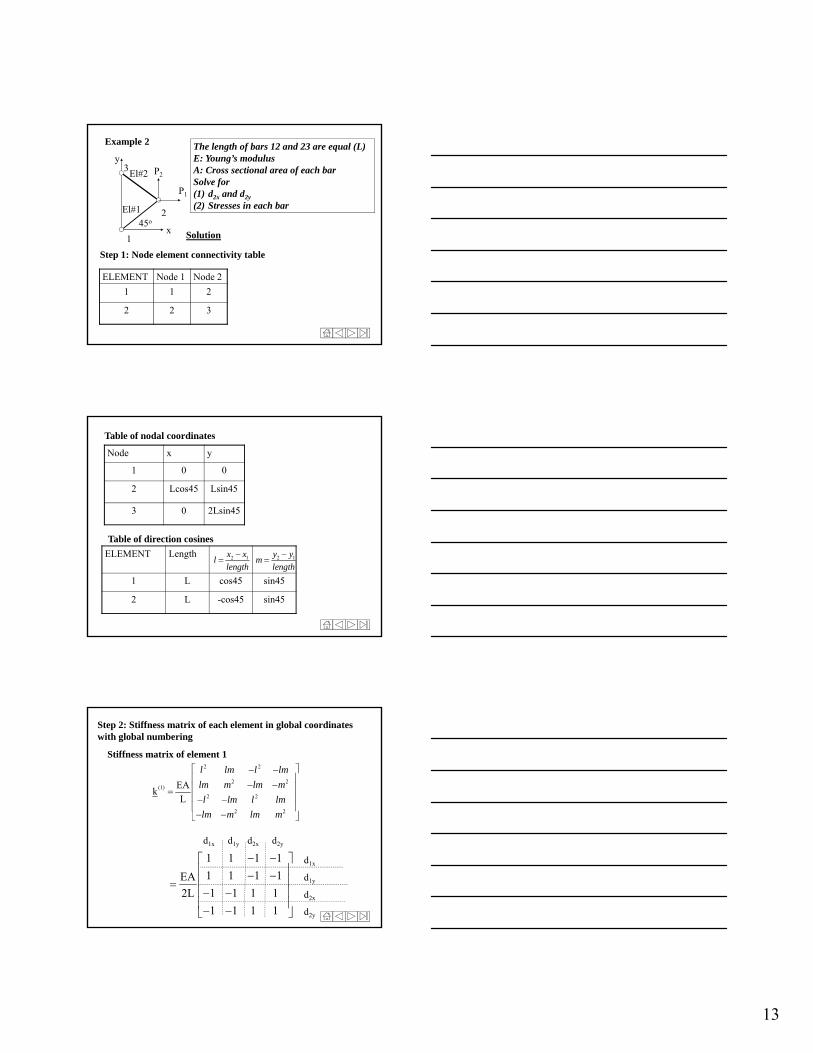
Example 2
P1
P2
2
3
x
y
El#1
El#2
The length of bars 12 and 23 are equal (L)E: Young’s modulusA: Cross sectional area of each barSolve for (1) d2x and d2y
(2) Stresses in each bar
Solution45o
1 Solution
Step 1: Node element connectivity table
ELEMENT Node 1 Node 2
1 1 2
2 2 3
Table of nodal coordinates
Node x y
1 0 0
2 Lcos45 Lsin45
3 0 2Lsin45
Table of direction cosines
ELEMENT Length
1 L cos45 sin45
2 L -cos45 sin45
2 1x xl
length
2 1y y
mlength
Step 2: Stiffness matrix of each element in global coordinates with global numbering
2 2
2 2(1)
2 2
2 2
EAk
L
l lm l lm
lm m lm m
l lm l lm
lm m lm m
Stiffness matrix of element 1
d1x
d2x
d2xd1x d1y d2y
d1y
d2y
1 1 1 1
1 1 1 1EA
1 1 1 12L
1 1 1 1
14
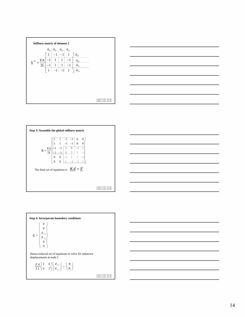
Stiffness matrix of element 2
d2x
d3x
d3x d3y
d2y
d3
d2x d2y
(2)
1 1 1 1
1 1 1 1EAk
1 1 1 12L
1 1 1 1
d3y1 1 1 1
1 1 1 1 0 0
1 1 1 1 0 0
1 1 2 0 1 1EAK
1 1 0 2 1 12L
0 0 1 1 1 1
Step 3: Assemble the global stiffness matrix
0 0 1 1 1 1
The final set of equations is K d F
Step 4: Incorporate boundary conditions
2
2
0
0
0
0
x
y
dd
d
0
Hence reduced set of equations to solve for unknown displacements at node 2
2 1
2 2
2 0
0 22x
y
d PE Ad PL

15
Step 5: Solve for unknown displacements
1
2
2 2
x
y
P Ld E Ad P L
E A
Step 6: Obtain stresses in the elements 0
For element #1: 1
1(1)
2
2
1 22 2
E 1 1 1 1
L 2 2 2 2
E( )
2L 2
x
y
x
y
x y
d
d
d
d
P Pd d
A
0
For element #2: 2
2(2)
3
3
1 22 2
E 1 1 1 1
L 2 2 2 2
E( )
2L 2
x
y
x
y
x y
d
d
d
d
P Pd d
A
0
0
2L 2A
Multi-point constraints
© 2002 Brooks/Cole Publishing / Thomson Learning™
Figure 3-19 Plane truss with inclined boundary conditions at node 3 (see problem worked out in class)

16
Problem 3: For the plane truss
P
2
3
y
El#1
El#2
El#3
P=1000 kN, L=length of elements 1 and 2 = 1mE=210 GPaA = 6×10⁻⁴m2 for elements 1 and 2
= 6 ×10⁻⁴ m2 for element 32
Determine the unknown displacements
1 x45o
Determine the unknown displacements and reaction forces.
Solution
Step 1: Node element connectivity table
ELEMENT Node 1 Node 2
1 1 2
2 2 3
3 1 3
Table of nodal coordinates
Node x y
1 0 0
2 0 L
3 L L
Table of direction cosines
ELEMENT Length
1 L 0 1
2 L 1 0
3 L
2 1x xl
length
2 1y y
mlength
2 1/ 2 1/ 2
Step 2: Stiffness matrix of each element in global coordinates with global numbering
2 2
2 2(1)
2 2
2 2
EAk
L
l lm l lm
lm m lm m
l lm l lm
lm m lm m
Stiffness matrix of element 1
d1x
d2x
d2xd1x d1y d2y
d1y
d2y
9 -4
0 0 0 0
0 1 0 1(210 10 )(6 10 )
0 0 0 01
0 1 0 1

17
Stiffness matrix of element 2
d2x
d3x
d3x d3y
d2y
d3y
d2x d2y
9 -4(2)
1 0 1 0
0 0 0 0(210 10 )(6 10 )k
1 0 1 01
0 0 0 0
Stiffness matrix of element 3Stiffness matrix of element 3
9 -4(3)
0.5 0.5 0.5 0.5
0.5 0.5 0.5 0.5(210 10 )(6 2 10 )k
0.5 0.5 0.5 0.52
0.5 0.5 0.5 0.5
d1x
d3x
d3x d3y
d1y
d3y
d1x d1y
5
0.5 0.5 0 0 0.5 0.5
0.5 1.5 0 1 0.5 0.5
0 0 1 0 1 0K 1260 10
0 1 0 1 0 0
0.5 0.5 1 0 1.5 0.5
0 5 0 5 0 0 0 5 0 5
Step 3: Assemble the global stiffness matrix
N/m
0.5 0.5 0 0 0.5 0.5
The final set of equations is K d F Eq(1)
Step 4: Incorporate boundary conditions
2
3
0
0
0x
x
dd
d
d
P
2
3
y
El#1
El#2
45o
El#3
xy
3 yd 1 x
45
Also, 3 0yd
How do I convert this to a boundary condition in the global (x,y) coordinates?
in the local coordinate system of element 3

18
1
1
2
3
x
y
y
x
F
F
PF
F
F
F
P
2
3
y
El#1
El#2
45o
El#3
xy
3 yF 1 x
45
Also, 3 0xF
How do I convert this to a boundary condition in the global (x,y) coordinates?
in the local coordinate system of element 3
3 3
33
1
2
x x
yy
dd l ml m
dm ld
Using coordinate transformations
3 33 3
33
1 1 1
2 2 21 1 1
x yx x
yy
d ddd
dd d d
33
3 32 2 2
yyy x
d d d
3 0yd
3 3 3
3 3
10
20
y y x
y x
d d d
d d
Eq (2)
(Multi-point constraint)
3 3
33
1
2
x x
yy
FF l ml m
Fm nF
Similarly for the forces at node 3
3 33 3
33
1 1 1
2 2 21 1 1
x yx x
yy
F FFF
FF F F
33
3 32 2 2
yyy x
F F F
3 3 3
3 3
10
20
x y x
y x
F F F
F F
Eq (3)
3 0xF
19
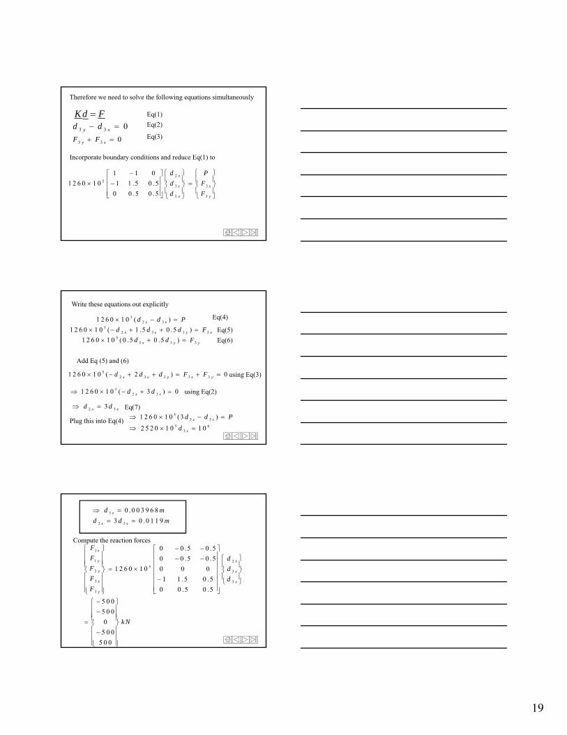
Therefore we need to solve the following equations simultaneously
K d F Eq(1)
3 3 0y xd d Eq(2)
3 3 0y xF F Eq(3)
Incorporate boundary conditions and reduce Eq(1) to
25
3 3
3 3
1 1 0
1 2 6 0 1 0 1 1 .5 0 .5
0 0 .5 0 .5
x
x x
y y
d P
d F
d F
Write these equations out explicitly
52 3
52 3 3 3
53 3 3
1 2 6 0 1 0 ( )
1 2 6 0 1 0 ( 1 .5 0 .5 )
1 2 6 0 1 0 ( 0 .5 0 .5 )
x x
x x y x
x y y
d d P
d d d F
d d F
Eq(4)
Eq(5)
Eq(6)
Add Eq (5) and (6)
52 3 3 3 31 2 6 0 1 0 ( 2 ) 0x x y x yd d d F F using Eq(3)
52 31 2 6 0 1 0 ( 3 ) 0x xd d using Eq(2)
2 33x xd d Eq(7)
Plug this into Eq(4)5
3 3
5 63
1 2 6 0 1 0 (3 )
2 5 2 0 1 0 1 0
x x
x
d d P
d
3
2 3
0 .0 0 3 9 6 8
3 0 .0 1 1 9x
x x
d m
d d m
Compute the reaction forces1
1 25
2 3
0 0 .5 0 .5
0 0 .5 0 .5
1 2 6 0 1 0 0 0 0
x
y x
y
F
F d
F d
2 3
3 3
3
1 2 6 0 1 0 0 0 0
1 1 .5 0 .5
0 0 .5 0 .5
5 0 0
5 0 0
0
5 0 0
5 0 0
y x
x y
y
d
F d
F
k N

20
Physical significance of the stiffness matrix
In general, we will have a stiffness matrix of the form
232221
131211
kkk
kkk
kkk
K
333231 kkk
And the finite element force-displacement relation
3
2
1
3
2
1
333231
232221
131211
F
F
F
d
d
d
kkk
kkk
kkk
Physical significance of the stiffness matrix
The first equation is
1313212111 Fdkdkdk Force equilibrium equation at node 1
Columns of the global stiffness matrix
What if d1=1, d2=0, d3=0 ?
313
212
111
kF
kF
kF
Force along d.o.f 1 due to unit displacement at d.o.f 1
Force along d.o.f 2 due to unit displacement at d.o.f 1Force along d.o.f 3 due to unit displacement at d.o.f 1
While d.o.f 2 and 3 are held fixed
Similarly we obtain the physical significance of the other entries of the global stiffness matrix
ijk = Force at d.o.f ‘i’ due to unit displacement at d.o.f ‘j’keeping all the other d.o.fs fixed
In general
21
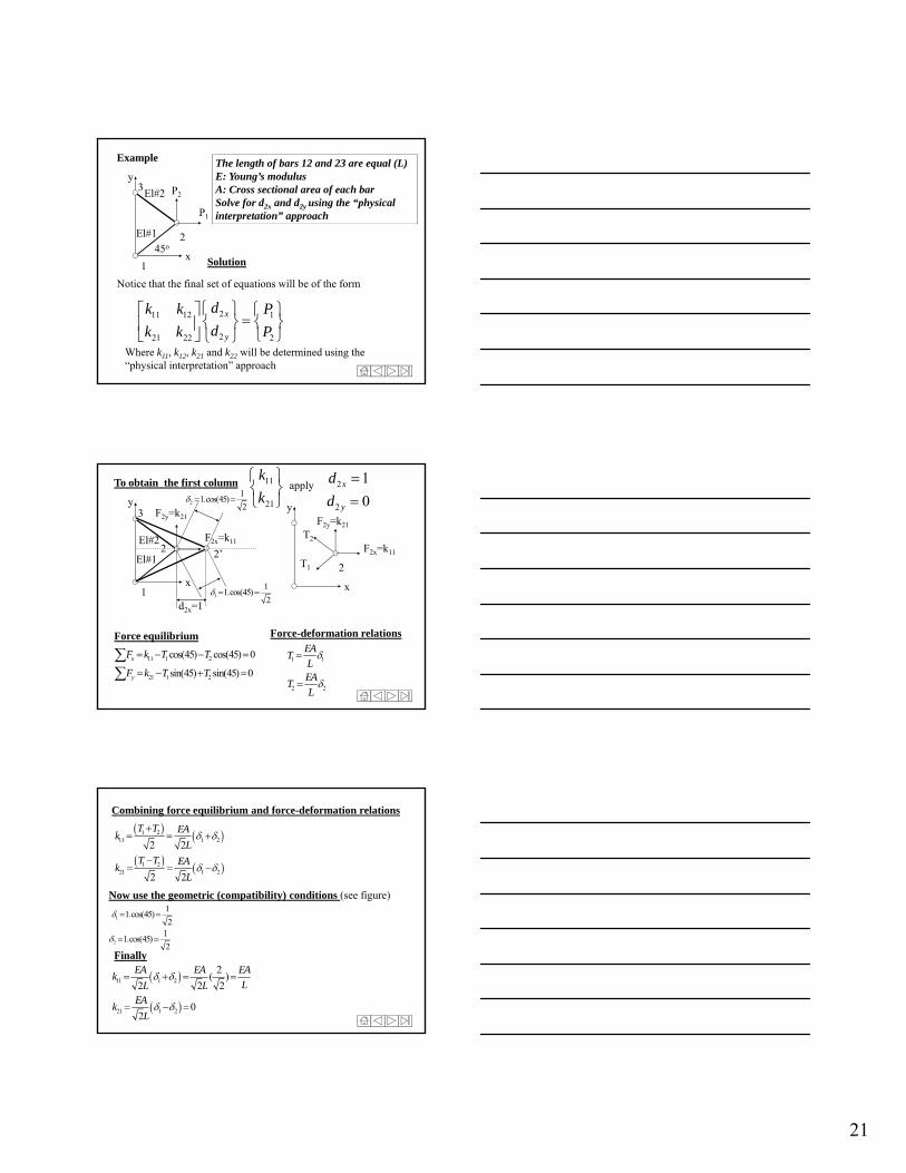
Example
P1
P2
2
3
x
y
El#1
El#2
The length of bars 12 and 23 are equal (L)E: Young’s modulusA: Cross sectional area of each barSolve for d2x and d2y using the “physical interpretation” approach
Solution45o
1 Solution
Notice that the final set of equations will be of the form
211 12 1
221 22 2
x
y
dk k P
dk k P
Where k11, k12, k21 and k22 will be determined using the “physical interpretation” approach
F2x=k11
F2y=k21
2
3
x
y
El#1
El#2
To obtain the first column 11
21
k
k
apply 2
2
1
0x
y
d
d
2
x
T1
y
2’
1
2
11.cos(45)
2
T2
F2x=k11
F2y=k21
1 x1
11.cos(45)
2
Force equilibrium
11 1 2
21 1 2
cos(45) cos(45) 0
sin(45) sin(45) 0
x
y
F k T T
F k T T
Force-deformation relations
1 1
2 2
EAT
LEA
TL
d2x=1
Combining force equilibrium and force-deformation relations
1 211 1 2
1 221 1 2
2 2
2 2
T T EAk
L
T T EAk
L
Now use the geometric (compatibility) conditions (see figure)1
1 (4 )
2
11.cos(45)
2
1
11.cos(45)
2
Finally
11 1 2
21 1 2
2( )
2 2 2
02
EA EA EAk
LL LEA
kL

22
2
3
x
y
El#1
El#2
To obtain the second column 12
22
k
k
apply 2
2
0
1x
y
d
d
2
x
T1
y
2’
1
2
11.cos(45)
2
T2
F2x=k12
F2y=k22
d2y=1
1 x1
11.cos(45)
2
Force equilibrium
12 1 2
22 1 2
cos(45) cos(45) 0
sin(45) sin(45) 0
x
y
F k T T
F k T T
Force-deformation relations
1 1
2 2
EAT
LEA
TL
Combining force equilibrium and force-deformation relations
1 212 1 2
1 222 1 2
2 2
2 2
T T EAk
L
T T EAk
L
Now use the geometric (compatibility) conditions (see figure)1
1 (4 )
2
11.cos(45)
2
1
11.cos(45)
2
Finally
12 1 2
22 1 2
02
2( )
2 2 2
EAk
LEA EA EA
kLL L
This negative is due to compression
© 2002 Brooks/Cole Publishing / Thomson Learning™ 3D Truss (space truss)
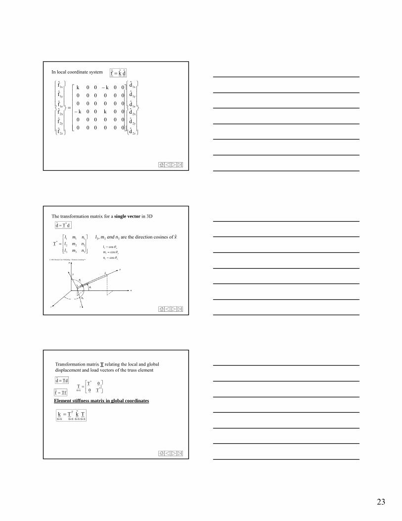
23
2x
1z
1y
1x
2x
1z
1y
1x
d
d
d
d
00k00k
000000
000000
00k00k
f
f
f
f
dkf In local coordinate system
2z
2y
2z
2y
d
d000000
000000
f
f
The transformation matrix for a single vector in 3D
333
222
111*T
nml
nml
nml
dTd *
l1, m1 and n1 are the direction cosines of x
z
y
x
n
m
l
cos
cos
cos
1
1
1
© 2002 Brooks/Cole Publishing / Thomson Learning™g g
Transformation matrix T relating the local and global displacement and load vectors of the truss element
dTd
*
*
66 T0
0TT
fTf
Element stiffness matrix in global coordinates
66666666TkTk
T
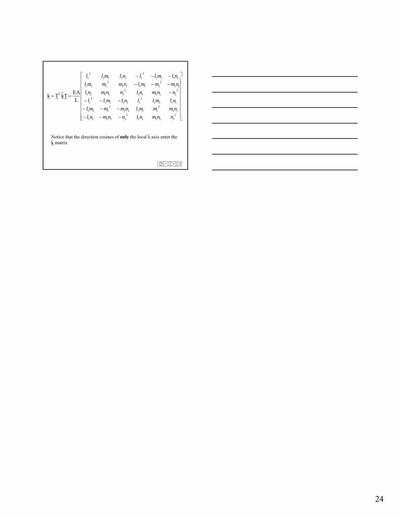
24
2211
211111
2111
11112
111112
1
211111
211111
112
111112
111
11112
111112
1
L
EATkTk
ll
nmmmlnmmml
nlmllnlmll
nnmnlnnmnl
nmmmlnmmml
nlmllnlmll
T
211111
211111 nnmnlnnmnl
Notice that the direction cosines of only the local x axis enter the k matrix
^


