
research for winter highway maintenance
Project 06428/CR14-02 November 2017
Pooled Fund #TPF-5(218)www.clearroads.org
Quantifying the Impact that New Capital Projects Will Have on Roadway
Snow and Ice Control OperationsTransportation Research Center
University of Vermont

Technical Report Documentation Page 1. Report No. 2. Government Accession No 3. Recipients Accession No.
CR 14-02
4. Title and Subtitle 5. Report Date
Quantifying the Impact that New Capital Projects Will Have on
Roadway Snow and Ice Control Operations
November 2017 6. Performing Organization Code
7. Author(s) 8. Performing Organization Report No.
James Sullivan, Jonathan Dowds, David C. Novak, Darren Scott, and Cliff Ragsdale
CR 14-02
9. Performing Organization Name and Address 10. Project/Task/Work Unit No.
Transportation Research Center University of Vermont, Farrell Hall 210 Colchester Ave. Burlington, Vermont 05405
11. Contract (C) or Grant (G) No.
MnDOT No. 06428
12. Sponsoring Organization Name and Address 13. Type of Report and Period Covered
Clear Roads Pooled Fund Study Lead State: Minnesota Department of Transportation Research Services & Library 395 John Ireland Boulevard, MS 330 St. Paul, Minnesota 55155-1899
Final report [June 1, 2015 – November 30,
2017] 14. Sponsoring Agency Code
15. Supplementary Notes
Project completed for Clear Roads Pooled Fund program, TPF-5(218). See www.clearroads.org. 16. Abstract (Limit: 250 words)
In recent years, many states have experienced heavy burdens on their snow and ice control budgets. Increases in winter/spring precipitation results in increased costs to state DOTs for winter roadway maintenance materials (salt, sand, chemicals, etc.), plow operator time, equipment maintenance and replacement budgets, and fuel use. As state DOTs adjust to climate conditions that include not only more precipitation, but more severe and unpredictable weather events, it will become increasingly important to integrate the cost of roadway snow and ice control (RSIC) operations into their capital-project planning processes. The overall goal of this project was to support state DOTs’ operations & maintenance efforts by developing an automated method for quantifying the expected impact that new capital projects will have on RSIC operations. The effects of a new suburban roadway were found to be the most significant, requiring 266 vehicle-minutes of travel along with almost 40 minutes of additional service time or one additional fleet truck for each mile of new roadway. The results and findings of this research have implications for short-term funding allocations for RSIC operations staff and for long-term consideration of RSIC in the highway planning and design processes. The findings of this project provide defensible data for operations staff to advocate for increases in funding to offset the increased RSIC burden when a project is completed. The calculation tool created incorporates all of the results above into a MS Excel decision support platform, providing quick estimates of the monetary impact of a variety of major highway project types.
17. Document Analysis/Descriptors 18. Availability Statement
Roadway snow and ice control, burden, effort, routing, snow plow, fleet, optimization, winter maintenance, capital projects, budgeting
No restrictions. Document available from: National Technical Information Services, Alexandria, Virginia 22312
19. Security Class (this report) 20. Security Class (this page) 21. No. of Pages 22. Price
Unclassified Unclassified 57 -0-

Quantifying the Impact that New Capital Projects Will Have on
Roadway Snow and Ice Control Operations
FINAL REPORT
Prepared by:
James Sullivan
Jonathan Dowds
Transportation Research Center
University of Vermont
David C. Novak
School of Business
University of Vermont
Darren Scott
School of Geography & Earth Sciences
McMaster University
Cliff Ragsdale
College of Business
Virginia Polytechnic Institute and State University
November 2017
Published by:
Minnesota Department of Transportation
Research Services & Library
395 John Ireland Boulevard, MS 330
St. Paul, Minnesota 55155-1899
This report represents the results of research conducted by the authors and does not necessarily represent the views or policies
of the Minnesota Department of Transportation or the authors’ organizations. This report does not contain a standard or
specified technique.
The authors, the Minnesota Department of Transportation, and the authors’ organizations do not endorse products or
manufacturers. Trade or manufacturers’ names appear herein solely because they are considered essential to this report
because they are considered essential to this report.

ACKNOWLEDGMENTS
The authors of this report would like to acknowledge the Clear Roads national research consortium for
funding the work. The authors would also like to thank the supervisors and drivers from Minnesota and
New Hampshire who participated in the study.
i
TABLE OF CONTENTS
Introduction ....................................................................................................................1
1.1 Goals of the Project ............................................................................................................................. 2
1.2 Background .......................................................................................................................................... 2
1.2.1 Statewide Travel Model ............................................................................................................... 3
1.2.2 The Network Robustness Index (NRI) Calculation Tool ............................................................... 4
1.2.3 The RSIC Allocation & Routing Tool ............................................................................................. 4
1.3 Report Summary.................................................................................................................................. 4
Data Used in this project .................................................................................................6
2.1 Survey Data Collection and Selection of Case Studies ........................................................................ 6
2.2 GPS Data Collection ............................................................................................................................. 9
2.3 NOAA Weather Data for Storm Identification .................................................................................. 13
2.4 Costs and Rates Used in the Calculation Tool ................................................................................... 14
Methodology ................................................................................................................ 16
3.1 GPS Data Analysis .............................................................................................................................. 16
3.2 Development and Application of the Integrated Roadway Snow & Ice Control Routing Model ..... 17
3.2.1 Map Layer Development............................................................................................................ 17
3.2.2 Integration of Models ................................................................................................................ 18
3.2.3 Integrated RSIC Model Case Study Application ......................................................................... 22
3.3 Calculation Tool Development .......................................................................................................... 23
Results .......................................................................................................................... 25
4.1 Increased RSIC Burden for The Roundabout in Lancaster, New Hampshire .................................... 25
4.2 Increased RSIC Burden for the Champlain Parkway in Burlington, Vermont ................................... 28
4.3 Increased RSIC Burden for the Crescent Connector in Essex Junction, Vermont ............................. 30

ii
4.4 Increased RSIC Burden from the Addition of Left-Turn Lanes on U.S. Route 2 in Colchester,
Vermont ................................................................................................................................................... 31
4.5 Increased RSIC Burden from the Addition of a Lane in Each Direction of State Route 100 in
WATERBURY, Vermont ............................................................................................................................ 33
4.6 Special Case Study for a Rural By-Pass in Bennington, Vermont ...................................................... 35
4.7 Summary of Results for Use in the Calculation Tool ......................................................................... 38
Conclusions and Recommendations ............................................................................... 41
REFERENCES .................................................................................................................................... 45
APPENDIX A Survey Responses ....................................................................................................... A-1
LIST OF FIGURES
Figure 1 Percentage Change in Very Heavy Precipitation (from the Third National Climate Assessment
Report, 2014) ................................................................................................................................................. 1
Figure 2 Zones and Road Network in the Vermont Travel Model ................................................................ 3
Figure 3 Iterative Procedure for RSIC Allocation & Routing ......................................................................... 5
Figure 4 Locations of initial 7 capital projects selected for case studies ...................................................... 8
Figure 5 GeoStats Download Utility............................................................................................................. 10
Figure 6 GPS data for the MN 371 Project in Nisswa, Pequot Lakes, and Jenkins, Minnesota .................. 11
Figure 7 GeoStats GeoLogger (l. to r.) datalogger, 12V adapter, and antenna ........................................... 12
Figure 8 The intersection of US 2 and US 3 in Lancaster, New Hampshire as a stop- and yield-controlled
intersection (a) and as a roundabout (b) ..................................................................................................... 12
Figure 9 GPS Data Points Corresponding to the RSIC Service of the Lancaster Roundabout .................... 13
Figure 10 Final 5 case studies (in red) selected for analysis with the RSIC model ..................................... 17
Figure 11 Roadways representing the Champlain Parkway project (in blue), as added to the routing
network (brown) .......................................................................................................................................... 18
Figure 12 Integrated RSIC Model capital project evaluation flowchart ..................................................... 22

iii
Figure 13 GPS data points within the 1 km buffer of the intersection for 2015-2016 (a) and 2016-2017 (b)
..................................................................................................................................................................... 27
Figure 14 Roadways representing the Crescent Connector project (in blue), as added to the routing
network (brown) .......................................................................................................................................... 30
Figure 15 Roadways representing the Left-Turn Lanes on U.S. Route 2 project (blue in the inset), as
added to the routing network (brown) ....................................................................................................... 31
Figure 16 Roadways representing the Addition of a Lane in Each Direction on U.S. Route 100 project (in
blue), as added to the routing network (brown) ......................................................................................... 33
Figure 17 Roadways representing the Southern Segment of the Bennington Bypass project (in blue), as
added to the routing network (brown) ....................................................................................................... 35
Figure 18 Roads that are not part of the state-maintained network (in green) are bypassed by the new
project (in blue) ........................................................................................................................................... 37
Figure 19 MS Excel Calculation Tool - User Data (a) and Decision Support Tool (b) .................................. 42
LIST OF TABLES
Table 1 Unit Costs and Average Rates Used for Default Values in the Calculation Tool............................ 14
Table 2 Storm Classifications Used in this Project ...................................................................................... 16
Table 3 Vermont RSIC Truck Table .............................................................................................................. 19
Table 4 Integrated RSIC Model application scenarios ................................................................................ 23
Table 5 Dates, durations and storm classification data for each RSIC trip in the GPS dataset .................. 25
Table 6 Average time and average speed of RSIC service by storm class .................................................. 27
Table 7 Average time and average speed of RSIC service by storm severity ............................................. 28
Table 8 Results of Integrated RSIC Model applications for the Champlain Parkway project..................... 29
Table 9 Results of Integrated RSIC Model applications for the Crescent Connector project .................... 30
Table 10 Results of Integrated RSIC Model applications for the U.S Route 2 Left-Turn Lanes project ..... 32
Table 11 Results of Integrated RSIC Model applications for the State Route 100 Lane Addition project . 34
Table 12 Results of Integrated RSIC Model applications for the Bennington Bypass project .................... 35

iv
Table 13 Summary of results of the Integrated RSIC Model applications for increased RSIC effort ......... 38
Table 14 Summary of results of the Integrated RSIC Model applications for increased allocation ........... 39
Table 15 Summary of results of the Integrated RSIC Model applications for increased service time ....... 40
Table 16 RSIC Considerations and Recommendations for Design of New Capital Projects ....................... 43
v
LIST OF ABBREVIATIONS
AASHTO – American Association of State Highway Transportation Officials
DOT – Department of transportation
GIS – geographic information system
GPS – global positioning system
HS – high-salt
LS – low-salt
NRI – Network Robustness Index
RSIC – Roadway snow and ice control
STIP – Statewide Transportation Improvement Program
TAZ – traffic analysis zone
USDOT – United States Department of Transportation
VHT – vehicle-hours of travel
E-1
EXECUTIVE SUMMARY
In recent years, many Snow Belt states have experienced heavy burdens on their RSIC budgets due to an
increase in extreme winter weather. Increases in winter/spring precipitation will result in increased
costs to state DOTs for winter roadway maintenance materials (salt, sand, chemicals, etc.), increased
plow operator time, increased equipment maintenance and replacement budgets, and increased fuel
use. As state DOTs adjust to climate conditions that include not only more precipitation, but more
severe and unpredictable weather events, it will become increasingly important to integrate the cost of
RSIC operations into their capital-project planning processes. The introduction of new capital projects
will obviously result in additional costs to state DOTs, as new projects increase the total effort and
expenditure needed for RSIC operations. It is the case; however, that the additional RSIC operations and
maintenance burden associated with new capital projects is rarely, if ever, quantified and is therefore
typically not considered during the early stages of the capital-project development process.
The overall goal of this project was to support state DOTs’ operations & maintenance efforts by
developing an automated method for quantifying the expected impact that new capital projects will
have on RSIC operations. The suggested approach emphasizes the need to explicitly consider RSIC-based
costs in the transportation project prioritization and climate adaptation planning processes, as RSIC
operations pose a large annual cost for many states.
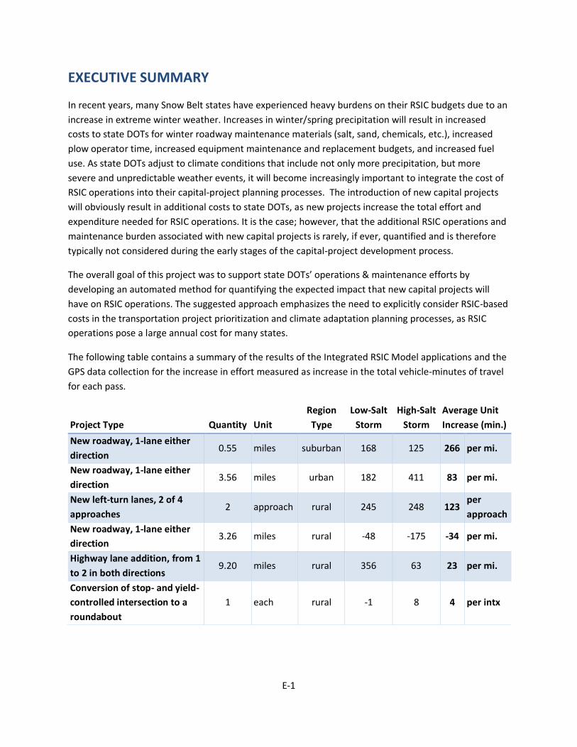
The following table contains a summary of the results of the Integrated RSIC Model applications and the
GPS data collection for the increase in effort measured as increase in the total vehicle-minutes of travel
for each pass.
Project Type Quantity Unit
Region
Type
Low-Salt
Storm
High-Salt
Storm
Average Unit
Increase (min.)
New roadway, 1-lane either
direction 0.55 miles suburban 168 125 266 per mi.
New roadway, 1-lane either
direction 3.56 miles urban 182 411 83 per mi.
New left-turn lanes, 2 of 4
approaches 2 approach rural 245 248 123
per
approach
New roadway, 1-lane either
direction 3.26 miles rural -48 -175 -34 per mi.
Highway lane addition, from 1
to 2 in both directions 9.20 miles rural 356 63 23 per mi.
Conversion of stop- and yield-
controlled intersection to a
roundabout
1 each rural -1 8 4 per intx

E-2
For each of these applications, the number of vehicles was held fixed, so the results assume that no new
vehicles (trucks or tow-plows) are added to the RSIC fleet. The effects of the new suburban roadway
were the most significant, as expected since the road network is less connected outside of the urban
core and there are fewer opportunities to devise an alternative set of efficient routes with the new
roadway. Adding left-turn lanes to a rural intersection approach also had a significant effect on RSIC
effort. These types of intersection improvements are common in rural and suburban areas where right-
of-way is available for the addition of turning lanes, but their considerable effect on RSIC effort must be
considered, especially in relation to the more moderate effect of converting a rural intersection to a
roundabout.
The following table contains a summary of the increase in vehicles allocated to the garage where each
project is located.
Project Type Quantity Unit
Region
Type
Low-Salt
Storm
High-Salt
Storm
Average Unit
Increase (trks)
New roadway, 1-lane either
direction 0.55 miles suburban 1 0 0.91 per mi.
New roadway, 1-lane either
direction 3.56 miles urban 1.5 1 0.35 per mi.
New left-turn lanes, 2 of 4
approaches 2 approach rural 0.5 0.5 0.25
per
approach
New roadway, 1-lane either
direction 3.26 miles rural 1 1 0.31 per mi.
Highway lane addition, from 1
to 2 in both directions 9.20 miles rural 1 2 0.16 per mi.
Conversion of stop- and yield-
controlled intersection to a
roundabout
1 each rural -- -- 1* per intx
As with the measured increases in effort, the effects of the new suburban roadway were the most
significant, requiring almost 1 additional truck for each mile of new roadway. Lane additions were
shown to have less of a need for additional trucks. Unless the new turn lanes are close to a garage,
having a new vehicle deadheading through the network to reach the new lanes will rarely be efficient.
Although the field data analysis was not able to identify the potential need for additional vehicles, it is
possible that a roundabout will require a new vehicle simply because its configuration precludes the use
of some heavier trucks.

E-3
The following table contains a summary of the increase in service time on the network, or the time it will
take to complete a single pass across all state-maintained roadways.
Project Type Quantity Unit
Region
Type
Low-Salt
Storm
High-Salt
Storm
Average Unit
Increase (min.)
New roadway, 1-lane either
direction 0.55 miles suburban 8 35 39 per mi.
New roadway, 1-lane either
direction 3.56 miles urban 9 38 7 per mi.
New left-turn lanes, 2 of 4
approaches 2 approach rural 14 0 4
per
approach
New roadway, 1-lane either
direction 3.26 miles rural 12 0 2 per mi.
Highway lane addition, from 1
to 2 in both directions 9.20 miles rural 5 16 1 per mi.
Conversion of stop- and yield-
controlled intersection to a
roundabout
1 each rural -- -- 0 per intx.
As with the other measures of RSIC burden, the effects of the new suburban roadway were the most
significant, requiring almost 40 minutes of additional service time for each mile of new roadway. The
other projects were shown to have a minimal effect on service time, especially in the high-salt storm
scenario, when the longest service time was likely to have been at a garage that was elsewhere on the
network, so the statewide service time did not change.
The results and findings of this research have implications for short-term funding allocations for RSIC
operations staff and for long-term consideration of RSIC in the highway planning and design processes.
The findings of this project provide defensible data for operations staff to advocate for increases in
funding to offset the increased RSIC burden when a project is completed. The calculation tool created
incorporates all of the results above into a MS Excel decision support platform, providing quick
estimates of the monetary impact of a variety of major highway project types.
These findings also provide a strong argument for the increased need to involve RSIC operations staff in
the highway planning and design processes for major capital projects. The ultimate long-term goal is for
the geometric design of highways to fully consider the impacts on all operations & maintenance needs,
including RSIC.
1
INTRODUCTION
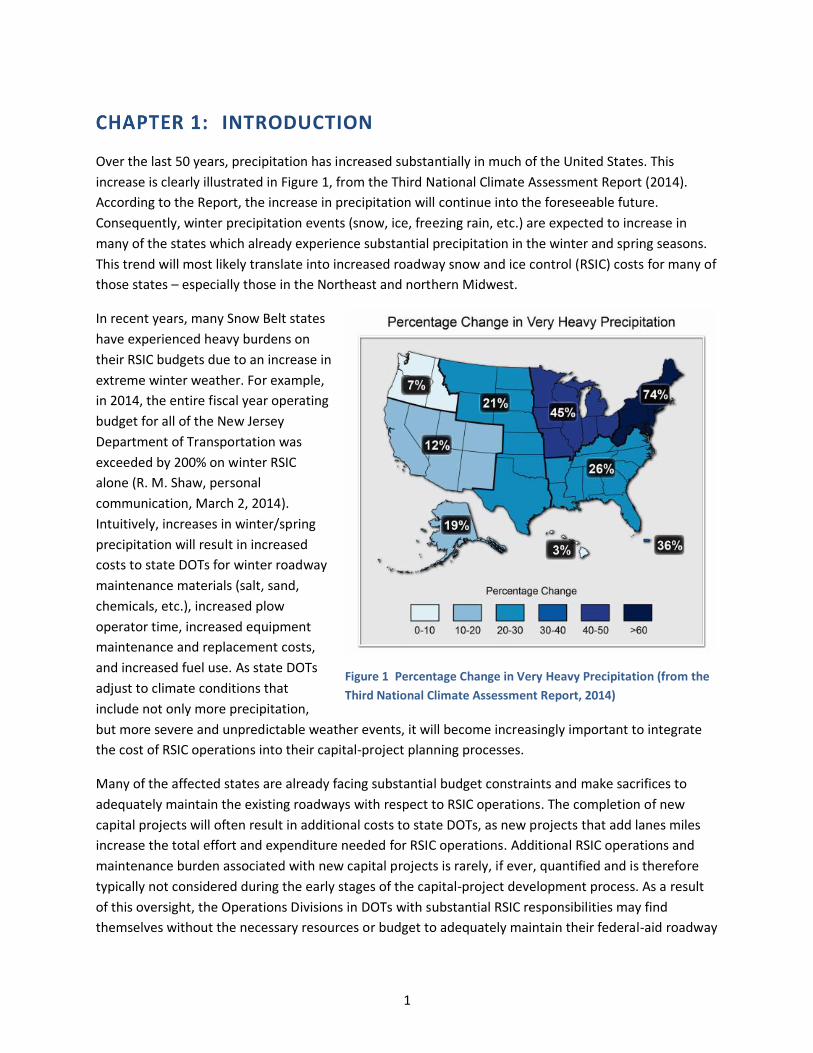
Over the last 50 years, precipitation has increased substantially in much of the United States. This
increase is clearly illustrated in Figure 1, from the Third National Climate Assessment Report (2014).
According to the Report, the increase in precipitation will continue into the foreseeable future.
Consequently, winter precipitation events (snow, ice, freezing rain, etc.) are expected to increase in
many of the states which already experience substantial precipitation in the winter and spring seasons.
This trend will most likely translate into increased roadway snow and ice control (RSIC) costs for many of
those states – especially those in the Northeast and northern Midwest.
In recent years, many Snow Belt states
have experienced heavy burdens on
their RSIC budgets due to an increase in
extreme winter weather. For example,
in 2014, the entire fiscal year operating
budget for all of the New Jersey
Department of Transportation was
exceeded by 200% on winter RSIC
alone (R. M. Shaw, personal
communication, March 2, 2014).
Intuitively, increases in winter/spring
precipitation will result in increased
costs to state DOTs for winter roadway
maintenance materials (salt, sand,
chemicals, etc.), increased plow
operator time, increased equipment
maintenance and replacement costs,
and increased fuel use. As state DOTs
adjust to climate conditions that
include not only more precipitation,
but more severe and unpredictable weather events, it will become increasingly important to integrate
the cost of RSIC operations into their capital-project planning processes.
Many of the affected states are already facing substantial budget constraints and make sacrifices to
adequately maintain the existing roadways with respect to RSIC operations. The completion of new
capital projects will often result in additional costs to state DOTs, as new projects that add lanes miles
increase the total effort and expenditure needed for RSIC operations. Additional RSIC operations and
maintenance burden associated with new capital projects is rarely, if ever, quantified and is therefore
typically not considered during the early stages of the capital-project development process. As a result
of this oversight, the Operations Divisions in DOTs with substantial RSIC responsibilities may find
themselves without the necessary resources or budget to adequately maintain their federal-aid roadway
Figure 1 Percentage Change in Very Heavy Precipitation (from the
Third National Climate Assessment Report, 2014)

2
network in winter/spring months. In turn, this can have a negative impact on both safety and mobility
within those states.
1.1 GOALS OF THE PROJECT
The overall goal of this project was to support state DOTs’ operations and maintenance efforts by
developing an automated method for quantifying the expected impact that new capital projects will
have on RSIC operations. The suggested approach emphasizes the need to explicitly consider RSIC-based
costs in the transportation project prioritization and climate adaptation planning processes, as RSIC
operations pose a large annual cost for many states. For this project, we examined two general
categories of new capital projects to assess their impact on RSIC operations:
• Additions of new roadway capacity including new lanes, new shoulders, as well as new roadway
builds
• New roadway configurations such as new striping plans, new curb-cuts, new bulb-outs, bike
lanes, etc.
The research team developed a methodological approach to quantify the impact that new capital
projects will have on total vehicle-hours of travel (VHTs) and equipment needs for the RSIC fleet.
1.2 BACKGROUND
The team extended an existing RSIC allocation and routing tool that was developed in a previous project
funded by VTrans into a fully Integrated RSIC Model. The current tool is used to plan the most effective
routes for a RSIC fleet by minimizing total operating hours and fuel. It can also provide RSIC service
according to a roadway prioritization hierarchy (i.e., serving the highest priority roadways first). For this
project, the team expanded the functionality of the tool by integrating it with a travel model and a tool
for calculating the criticality of network links.
The importance of developing an integrated model to understand the effects of a new roadway
configuration comes from a need to better understand the “ripple” effects that an increase in a fleet’s
RSIC burden can have. The localized impact of a new capital project might include the need for a specific
driver to spend more time providing service to a new roadway segment, or an existing roadway segment
that has been changed, or the need for a different piece of equipment to provide service when a change
has been made. However, these changes will not only affect that specific driver and their route, but are
likely to impact the rest of the district, and the entire RSIC fleet. It is likely that changes will need to be
made to other routes to equalize the RSIC burden and continue to provide services in an efficient
manner. It is also possible that RSIC vehicles will need to be moved from one district to another to meet
the new demand caused by different capital projects. The indirect “ripple” effects throughout the state’s
network can be the most substantial costs resulting from a new roadway configuration, so it is critical
that they be considered.

3
1.2.1 Statewide Travel Model
Travel models are detailed GIS-based planning tools that can be used to provide projections of everyday
travel-behavior under a variety of scenarios for transportation planning studies, such as adding a new
capital project to the federal-aid roadway network. The outputs provided by these models are used to
facilitate accurate and timely travel forecasts as well as to gain a better understanding of the current
operational status of existing transportation systems, which helps direct funding and policy decisions.
Vermont’s statewide travel
model is a series of spatial
computer processes that use
land-use and activity patterns
to estimate travelers’ behaviors
on a typical day. Origin and
destination tables are created,
describing the number of
expected trips between traffic
analysis zones (TAZs).
Accommodations are made for
commercial-truck trips and the
occupancy characteristics of
passenger vehicles. The final
outputs are traffic volumes by
roadway link on the statewide
federal-aid roadway network.
The Vermont Travel Model
currently includes 936 TAZs and
5,327 miles (see Figure 2).
Figure 2 Zones and Road Network in the Vermont Travel Model

4
1.2.2 The Network Robustness Index (NRI) Calculation Tool
The Network Robustness Index (NRI), is a performance measure for evaluating the importance of a given
roadway segment (i.e., network link) with respect to the entire roadway network. The NRI is based on
the change in travel-times associated with re-routing all traffic in the network when a given roadway link
becomes unusable. Thus, the most important links in the network are the links: 1) that carry a relatively
high volume of traffic, and 2) lack nearby alternative routes. The algorithm for the NRI tool was first
developed in 2006 and it now allows the decision maker to differentiate the importance of different
types of vehicle trips by trip purpose, and is used to rank-order all links in the transportation network.
1.2.3 The RSIC Allocation & Routing Tool
The existing RSIC allocation and routing tool utilizes an innovative procedure for finding optimal routes
for a given fleet of RSIC vehicles, ensuring that each vehicle is utilized and total vehicle-hours of travel
are minimized. The procedure starts with a network that has been clustered into districts, and proceeds
by assigning each vehicle in the fleet to a district. This vehicle-allocation step is repeated after each
routing step so that none of the fleet is left idle (see Figure 3).
Each of the sub-components of the Integrated RSIC Model is built on the TransCAD® software platform.
TransCAD® is a Geographic Information System (GIS) designed specifically to store, display, manage, and
analyze transportation data. TransCAD® integrates GIS and transportation modeling into a single
platform, providing capabilities in mapping, visualization, and analysis with application modules for
routing, travel-demand forecasting, public transit, logistics, site location, and territory management.
1.3 REPORT SUMMARY
Chapter 2 of this report identifies and describes all of the data collected and used in this project. Section
3 provides a detailed description of the methods used to analyze data, including the development of the
Integrated RSIC Model and the Calculation Tool. Chapter 4 provides a summary of the results of those
analyses, and the application of the Integrated RSIC Model. Chapter 5 provides the conclusions of the
project and the recommendations for how those conclusions can be used to influence the way that
capital projects are developed.

5
Calculate garage-
specific "smart"
time windows
Capacitated
vehicle-routing
Increase time
window for
garages with
orphans by 5
minutes
YES
Do any of the
garages have
unserved road
segments?
NO
Shift idle vehicles
to garages in this
set with the largest
RSIC burden (RSIC
stress or salt ratio)
Select garages
which have not
already received a
re-allocated
vehicle and which
do not have an
idle vehicle
YES
Do any of the
garages have idle
vehicles?
NO
Garage-specific
"smart" time
windows and
vehicle allocations
Done - Use current vehicle
allocations and current set of
vehicle routes
begin or
endinput data
calculation
procedure
decision
point
TransCAD
procedure
Key
Figure 3 Iterative Procedure for RSIC Allocation & Routing

6
DATA USED IN THIS PROJECT
This section describes the data that was collected or gathered from other sources during the execution
of this project.
2.1 SURVEY DATA COLLECTION AND SELECTION OF CASE STUDIES
The first project task involved the preparation and distribution of a survey to decide on the types of
projects to be studied. The purpose of the survey was to solicit information on project types that are
common across the Clear Roads’ member states and which cause concern for RSIC burden. The survey
was distributed to the AASHTO RSIC ListServ in an email with the following text:
We are in the beginning stages of a project funded by the Clear Roads research program
that is aimed at measuring the increased burden on snow and ice control (SIC) that
results from new roadway configurations or expansions. We intend to examine 6-10
“case studies” featuring typical roadway projects that have an effect on the effort or
equipment required for SIC. An example would be changing a traditional signalized
intersection into a roundabout. We will measure the effort required before and after the
new configuration has been completed.
What we need are case studies to focus on in the 2016 construction season, so that we
can observe “before” conditions this winter season. So if you know of a project that is
being built or implemented in 2016 that is a concern for SIC, let us know! Also, let us
know if there is a general type of project that concerns you, even if you don’t know of
one being implemented in 2016.
Ideally, we would like to observe the pre- and post- implementation conditions first-
hand, but if your fleet stores historical AVL data, we may be able to use that to measure
the effort required for a project that has already been completed. So also let us know if
your agency logs and stores historical AVL data from your SIC fleet, even if it’s only last
winter.
Any input you can provide would be greatly appreciated.
The email responses received are compiled in Appendix A.
After following up on the projects suggested by the survey responders, it became clear that detailed
information on the full array of capital projects that suited the needs of this research was limited.
Therefore, it was very difficult for RSIC managers to identify capital projects with construction scheduled
in 2016 that would be completed by the winter of 2016/2017. Therefore, the investigation of potential
capital projects to use as case studies was shifted from the survey responses to a scan of the State
Transportation Improvement Programs (STIPs) for a subset of the Clear Roads member states
represented by the responders. The STIP is a staged, multi-year, statewide, intermodal program of
capital projects, funded by the USDOT. Federal requirements dictate that the STIP must cover a period
7
of not less than 4 years, it must be fiscally constrained by year and include financial information to
demonstrate which projects and project phases are to be implemented using yearly revenues.
STIP projections for 2016-2019 were scanned for projects with significant (> $10,000) construction
scheduled in FY2016 and no further construction planned in FY2017. The types of projects sought were
lane additions, roadway expansions (including complete streets and bike lane additions), roundabouts,
and bridge reconstructions. The case study investigation was focused on the states which responded to
the initial survey:
• Indiana
• Minnesota
• New Hampshire
• Maine
• Vermont
For Indiana, 17 possible capital projects were initially found which included added travel lanes, bridge
widening, and an intersection improvement with a roundabout. However, none of these projects could
be confirmed to be starting in FY2016 and completed by FY2017.
For Minnesota, 67 possible capital projects were initially found consisting of bridge replacements,
shoulder paving/widening, bike/ped improvements, and added turn lanes. From these, two candidates
for case-study analysis were selected because they seemed to fit the constraints of the project:
• MN 25/55: Reconstruction, widening, signalization, and addition of left-turn lanes at the
intersection of MN 25 & MN 55 and construction of a roundabout at the intersection of MN 25
and 8th St. in Buffalo
• MN 371: Four-lane expansion (from one lane in each direction to 2 lanes in each direction) of
MN 371 in Nisswa, Pequot Lakes, and Jenkins
For New Hampshire, 12 possible capital projects consisting of roadway widening (additional lanes),
addition of bike shoulders, bridge replacement, roadway reconstruction, and roundabout construction.
From these, two candidates for case-study analysis were selected:
• NH 108: Reconstruction of the roadway and addition of bike shoulders on NH 108 in Durham
and Newmarket
• NH Roundabout: Construction of a roundabout at the intersection of US 2 and US 3 in Lancaster
For Maine, the STIP was reviewed but the review did not uncover any new types of capital projects that
were not already covered by projects found in other states.
For Vermont, the STIP review only revealed 10 capital projects. In Vermont, extensive capital costs are
still being dedicated to repairs from Hurricane Irene. None of the projects investigated for Vermont was
scheduled to be completed by FY2017, but construction timing was not critical for Vermont because a

8
the Integrated RSIC Model was to be used. Therefore, the following 3 projects were selected for analysis
using the Vermont Integrated RSIC Model:
• CrCo: Construction of a new by-pass roadway (the Crescent Connector) between State Route 2A
and State Route 117, with improvements to Railroad St. between State Routes 15 and 117 in
Essex Junction
• Rt2Lefts: Construction of new left-turn lanes for US Route 2 traffic at its intersection with Clay
Point Road / Bear Trap Road in Colchester
• ChPa: Construction of a new roadway (the Champlain Parkway) from I-189 to Lakeside Ave. in
Burlington. The Champlain Parkway, formerly the ‘Southern Connector’ originated in the 1960’s
as a 4-lane, limited access highway to improve vehicular access between downtown Burlington
and I-89. Today’s 2-lane version, with a multi-modal design that includes significant stormwater,
bike/pedestrian, and traffic calming components, represents a fundamental departure from the
project’s distant origins.
Figure 4 shows the locations of the initial seven case-study capital projects selected for analysis.
An additional set of Vermont projects were selected as “reserve” case studies. These case studies were
chosen so that they could be used in case any of the other projects failed to obtain valid field data. With
Figure 4 Locations of initial seven capital projects selected for case studies

9
the collection of field GPS data, there is always a risk that projects will not yield usable data. So the
following projects were held as “reserve” case studies:
• The Southern Segment of the Bennington ByPass (BennBP): The proposed bypass of Bennington
originated in the 1950's and was studied for several decades as a complete bypass of downtown
Bennington, primarily for tourists wishing to access the ski areas east of Bennington. The 4.2-
mile Western Segment, stretching from Hoosick, NY westward to Route 7, was completed in
2004. The Northern Segment, linking US Route 7 with State Route 9 to the east of town, was
completed in 2014. The third and final segment is the Southern Segment, which will extend in
an arc from Route 9 southwest to Route 2.
• Resurfacing of State Route 100 between Waterbury and Stowe, Vermont, beginning at the US
Route 2 intersection and extending to the north 9.8 miles (Rt100LaneAdds): Although this
project does not include a lane expansion along its entire scope, it does include capacity
improvements and some Vermont residents have argued that it should also include a full lane
expansion, due to congestion problems related to winter tourism. Therefore, a multilane
expansion is envisioned here as a potential case study.
2.2 GPS DATA COLLECTION
For each of the case studies outside of Vermont, the truck responsible for servicing the roadway
affected by the construction was instrumented with a GPS device, the GeoStats GeoLogger, to obtain
detailed information on the effort required to service it, both before and after the construction project.
GPS devices were mailed to the district supervisors to put into the trucks where these projects would be
built for the winter of 2015-2016, then again for the winter of 2016-2017.
After the 2015-2016 winter, the GPS data were plotted and mapped to check their quality upon the
return of the devices. Data logged by the GPS devices were available for download using the download
utility provided by GeoStats (Figure 5).

10
Figure 5 GeoStats Download Utility
The “Save Interval” was set at 5 seconds, indicating that a GPS point would be logged every 5 seconds
while the vehicle was turned on. Although the device is capable of saving at 1-second intervals, 5
seconds was deemed sufficient for this study, and would ensure that a full winter of data could be
stored on the device. All data recorded to the GeoLogger were downloaded in a single file, containing
the following fields:
• Latitude – Latitude of the vehicle position
• Longitude – Longitude of the vehicle position
• Time – clock time (00:00:00)
• Date
• Speed – vehicle speed, in miles per hour
• Heading – direction of travel (0 to 360 degrees)
• Altitude – Altitude of the vehicle (feet above mean sea level)
• HDOP – horizontal dilution of precision, an indication of the quality of the lat/long results
11
• Satellites – the number of
satellite signals contributing
to the GPS point
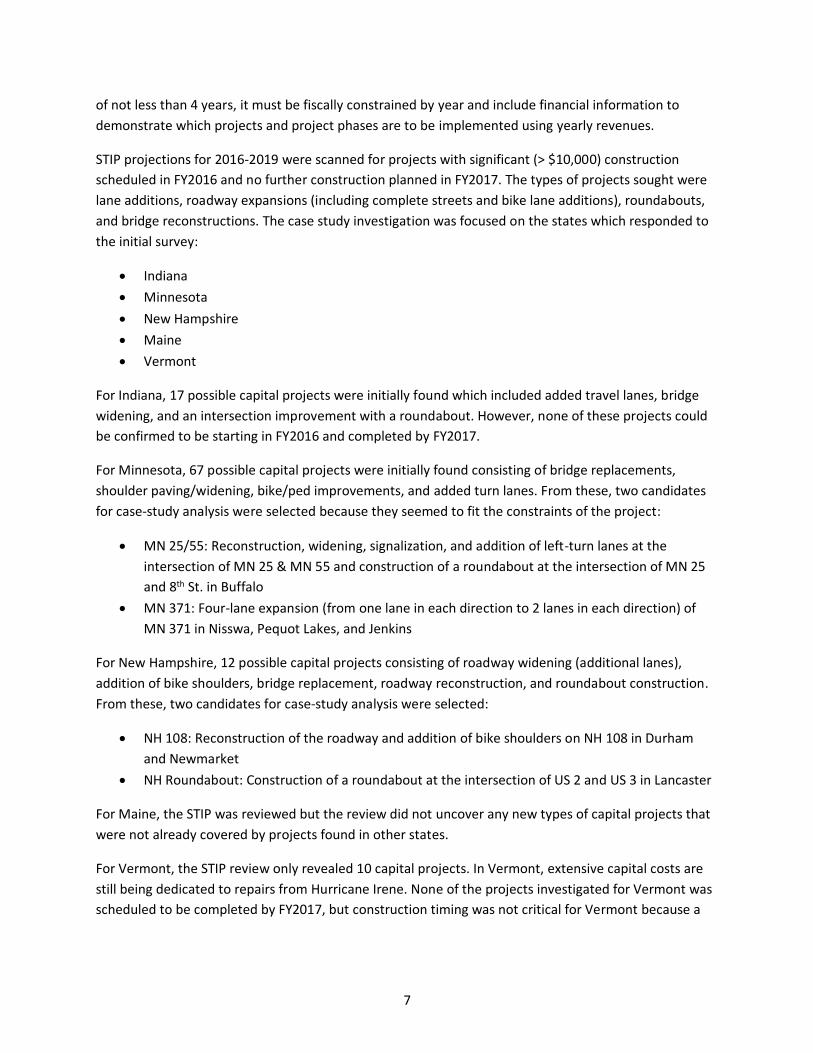
In all four cases for the 2015-2016
winter, the data were found to be
effective, and their spatial
representation coincided perfectly
with the expected route that the
vehicle was servicing. Figure 6
provides an example of the plotted
GPS data for the project on MN 371 in
Minnesota. The inset of Figure 6
verifies that the route indicated
consists of many individual GPS points
corresponding to the truck’s position
every 5 seconds.
Upon return of the GeoLogger devices
after the winter 2016-2017 data
collection, it was discovered that
three of the four devices contained no
data, making the use of these case
studies for analysis in this project
impossible. After reviewing the
procedures for shipping, installing, and
returning the devices, it was
determined that the most likely cause of the data deletion was contact with magnetic fields during
return shipping. Since the GeoLogger stores all of its data in flash memory, contact with, or proximity to,
a magnetic device causes loss of data. Unfortunately, the GeoLogger’s own antenna unit itself is
magnetic (Figure 7).
Figure 6 GPS data for the MN 371 Project in Nisswa, Pequot
Lakes, and Jenkins, Minnesota

12
In turn, this means that keeping the
antenna separated from the logger
during shipping is critical. An
envelope-type mailer was used for
return shipping for the first winter
data collection, making contact
between the antenna and the
logger difficult. However, due to
problems with the postage
requirements for the envelope-type
mailer, a larger box-type mailer was
used for return shipping for the
second winter data collection
event. The box-type mailer allowed
the antenna and the logger to
move around more freely within the
package.
Therefore, only one of the four case studies yielded usable data for both winter data collection periods.
This case study was the replacement of a traditional stop- and yield-controlled intersection at US 2 and
US 3 in Lancaster, New Hampshire (Figure 8a) with a roundabout (Figure 8b).
Figure 8 The intersection of US 2 and US 3 in Lancaster, New Hampshire as a stop- and yield-controlled
intersection (a) and as a roundabout (b)
a b
Figure 7 GeoStats GeoLogger (l. to r.) datalogger, 12V adapter, and
antenna
13
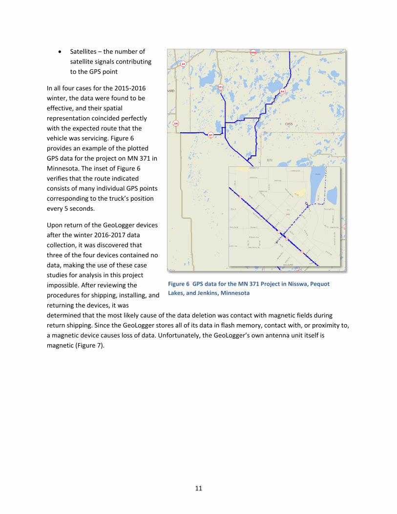
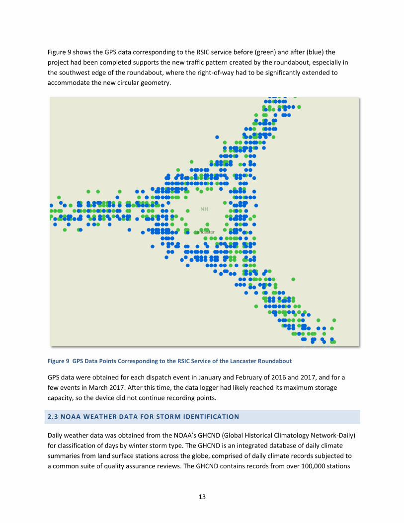
Figure 9 shows the GPS data corresponding to the RSIC service before (green) and after (blue) the
project had been completed supports the new traffic pattern created by the roundabout, especially in
the southwest edge of the roundabout, where the right-of-way had to be significantly extended to
accommodate the new circular geometry.
Figure 9 GPS Data Points Corresponding to the RSIC Service of the Lancaster Roundabout
GPS data were obtained for each dispatch event in January and February of 2016 and 2017, and for a
few events in March 2017. After this time, the data logger had likely reached its maximum storage
capacity, so the device did not continue recording points.
2.3 NOAA WEATHER DATA FOR STORM IDENTIFICATION
Daily weather data was obtained from the NOAA’s GHCND (Global Historical Climatology Network-Daily)
for classification of days by winter storm type. The GHCND is an integrated database of daily climate
summaries from land surface stations across the globe, comprised of daily climate records subjected to
a common suite of quality assurance reviews. The GHCND contains records from over 100,000 stations
14
in 180 countries and territories, including maximum and minimum temperature, total daily
precipitation, snowfall, and snow depth. For this project, GHCND data was obtained for every day of
January, February, and March of 2016 and 2017 for the Lancaster, New Hampshire weather station.
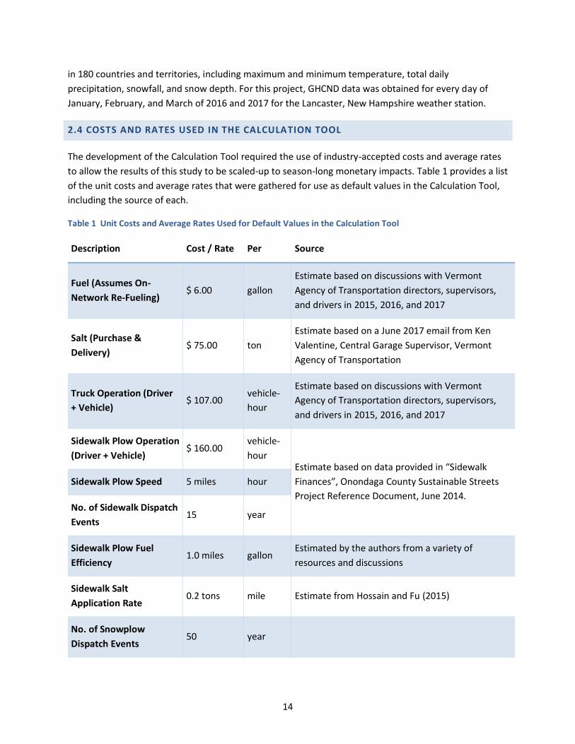
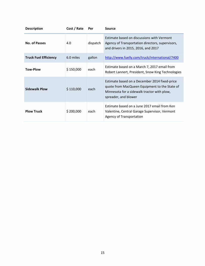
2.4 COSTS AND RATES USED IN THE CALCULATION TOOL
The development of the Calculation Tool required the use of industry-accepted costs and average rates
to allow the results of this study to be scaled-up to season-long monetary impacts. Table 1 provides a list
of the unit costs and average rates that were gathered for use as default values in the Calculation Tool,
including the source of each.
Table 1 Unit Costs and Average Rates Used for Default Values in the Calculation Tool
Description Cost / Rate Per Source
Fuel (Assumes On-
Network Re-Fueling) $ 6.00 gallon
Estimate based on discussions with Vermont
Agency of Transportation directors, supervisors,
and drivers in 2015, 2016, and 2017
Salt (Purchase &
Delivery) $ 75.00 ton
Estimate based on a June 2017 email from Ken
Valentine, Central Garage Supervisor, Vermont
Agency of Transportation
Truck Operation (Driver
+ Vehicle) $ 107.00
vehicle-
hour
Estimate based on discussions with Vermont
Agency of Transportation directors, supervisors,
and drivers in 2015, 2016, and 2017
Sidewalk Plow Operation
(Driver + Vehicle) $ 160.00
vehicle-
hour Estimate based on data provided in “Sidewalk
Finances”, Onondaga County Sustainable Streets
Project Reference Document, June 2014.
Sidewalk Plow Speed 5 miles hour
No. of Sidewalk Dispatch
Events 15 year
Sidewalk Plow Fuel
Efficiency 1.0 miles gallon
Estimated by the authors from a variety of
resources and discussions
Sidewalk Salt
Application Rate 0.2 tons mile Estimate from Hossain and Fu (2015)
No. of Snowplow
Dispatch Events 50 year
15
Description Cost / Rate Per Source
No. of Passes 4.0 dispatch
Estimate based on discussions with Vermont
Agency of Transportation directors, supervisors,
and drivers in 2015, 2016, and 2017
Truck Fuel Efficiency 6.0 miles gallon http://www.fuelly.com/truck/international/7400
Tow-Plow $ 150,000 each Estimate based on a March 7, 2017 email from
Robert Lannert, President, Snow King Technologies
Sidewalk Plow $ 110,000 each
Estimate based on a December 2014 fixed-price
quote from MacQueen Equipment to the State of
Minnesota for a sidewalk tractor with plow,
spreader, and blower
Plow Truck $ 200,000 each
Estimate based on a June 2017 email from Ken
Valentine, Central Garage Supervisor, Vermont
Agency of Transportation

16
METHODOLOGY
3.1 GPS DATA ANALYSIS
The GPS data points for 2016 and 2017 were compared using the date and time fields to assemble the
points into trips, so that each point was assigned to a specific trip. These trips correspond to passes of
the RSIC vehicle through the construction area. The elapsed time between points was used to assign
them to trip segments. For the Lancaster Roundabout project, a 1-km buffer was created around the
intersection to limit the set of points for analysis, and the average speed of the RSIC vehicle and the
average time through the construction area were calculated for each trip segment, and trip segments
were grouped by day for connection to storm events.
Daily weather from NOAA was used to classify storm intensities. The meteorological data were used to
create a simple storm classification based on Nixon and Qiu (2005) so that each trip segment could be
assigned to a specific type of storm. Each trip was assigned a storm classification based on the
temperature and precipitation classes used by Nixon and Qiu (2005), shown in Table 2.
Table 2 Storm Classifications Used in this Project
Storm Class Precipitation Class (Based on Snowfall Depth)
Temperature Class (Based on Daily Max. Temp.)
1 Light snow (< 2 in.) Warm (> 32 F)
2 Light snow (< 2 in.) Mid-Range (25 to 32 F)
3 Light snow (< 2 in.) Cold (< 25 F)
4 Medium snow (2- 6 in.) Warm (> 32 F)
5 Medium snow (2- 6 in.) Mid-Range (25 to 32 F)
It should be noted that the daily maximum temperature was used in the derivation of the classification
scheme and not the daily minimum or a calculated average temperature. In order to align these storm
classes with the “low-salt” and “high-salt” storm intensities used in the Integrated RSIC Routing Model,
classes 1 and 3 were aggregated as “low-salt” storms, and classes 2, 4, and 5 were aggregated as “high-
salt” storms.

17
3.2 DEVELOPMENT AND APPLICATION OF THE INTEGRATED ROADWAY SNOW & ICE
CONTROL ROUTING MODEL
The integration of the three tools was accomplished by adding computer code to the existing RSIC
allocation and routing tool to run the other tools in a logical sequence. The existing computer code was
also streamlined so that the entire process could be run in TransCAD, without the need for additional
coding or model platforms.
3.2.1 Map Layer Development
The base node/link layer for this
project was the snowplow routing
network used in previous projects
for Vermont, consisting of all roads
and highways in the statewide
travel model network. A variety of
additional updates were made to
this road network – new fields,
new roadways, new turnarounds,
and updates to the list of “stops”
to be serviced. New turnarounds
were added on I-89 in Burlington,
on I-93 at Exit 1, at the intersection
of State Route 279 and U.S. Route
7, and along U.S Route 4 at Exits 3,
4, 5 and 6. Two new attributes
were added to the road layer, one
to represent the Id field of the
original, un-split link, and the other
to represent the in-state length of
a roadway that crosses the
Vermont border. This step was
necessary to avoid allocating
vehicles to a garage based on
roadway length that the state is
not responsible for. In the routing
model, roadways are represented
as “stops” where salt is
“delivered”, at rate of either 200
lbs/mile (low-salt) or 500 lbs/mile
(high-salt).
Figure 10 Final 5 case studies (in red) selected for analysis with the
RSIC model
18
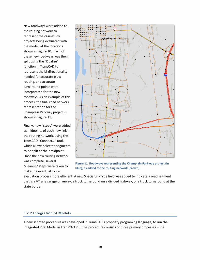
New roadways were added to
the routing network to
represent the case-study
projects being evaluated with
the model, at the locations
shown in Figure 10. Each of
these new roadways was then
split using the “Dualize”
function in TransCAD to
represent the bi-directionality
needed for accurate plow
routing, and accurate
turnaround points were
incorporated for the new
roadways. As an example of this
process, the final road network
representation for the
Champlain Parkway project is
shown in Figure 11.
Finally, new “stops” were added
as midpoints of each new link in
the routing network, using the
TransCAD “Connect…” tool,
which allows selected segments
to be split at their midpoint.
Once the new routing network
was complete, several
“cleanup” steps were taken to
make the eventual route
evaluation process more efficient. A new SpecialLinkType field was added to indicate a road segment
that is a VTrans garage driveway, a truck turnaround on a divided highway, or a truck turnaround at the
state border.
3.2.2 Integration of Models
A new scripted procedure was developed in TransCAD’s propriety programing language, to run the
Integrated RSIC Model in TransCAD 7.0. The procedure consists of three primary processes – the
Figure 11 Roadways representing the Champlain Parkway project (in
blue), as added to the routing network (brown)

19
network clustering and initial truck allocation, the route design, and the route evaluation & re-
allocation. The procedure is initiated once the following parameters have been specified:
• Storm Intensity – low-salt (LS): 200 lbs/mile or high-salt (HS): 500 lbs/mile
• Road Network Scenario – normal (“full”) or omitting the project in question
• Allocation Method – by miles of roadway each depot is responsible for, or by roadway criticality
each depot is responsible for
The procedure is initiated by calculating the total miles of roadway or the roadway criticality (as
measured by the Network Robustness Index, or NRI) that each garage is responsible for servicing.
Garages act as “Depots” for the routing procedure, providing a starting/ending point for all routes, as
well as a source of salt resupply. The initial allocation begins using the official truck table for Vermont’s
fleet, consisting of the detailed description of every truck used for RSIC in the state (Table 3).
Table 3 Vermont RSIC Truck Table
Type Count Make & Models
Average Model
Year
Salt Capacity
(tons)
1 10 International 4400, 4700, 4900, and 7300 2004 2.5
2 34 International 7400 2011 6
3 111 International 7400, 7500 2005 7.5
4 3 International 7600 6X4 2009 7.8
5 12 International 7500 2008 8.3
6 19 International 7600 2012 9.9
7 60 International 2574, 7600 2006 14.4
To determine the number of trucks allocated to each garage, the garage’s share of statewide roadway
mileage or roadway criticality (NRI times length) is calculated and that fraction of the total RSIC fleet is
allocated to the garage. For example, in a state with 5,000 miles of roadway, a garage responsible for
500 miles of roadway would be assigned 10% of its RSIC truck fleet (500/5,000). The only exception to
this calculation is that each garage is guaranteed at least one truck. If a garage’s allocation percentage
would yield less than 1 truck, its allocation is rounded up to 1.
Once each garage’s share of the statewide RSIC fleet is determined, specific trucks are assigned from the
official truck table, beginning with the highest capacity trucks (Type 7) in the fleet and proceeding to the
lowest capacity. In this way, garages with only one truck are ensured a Type 7 truck, and garages with
many trucks get a variety of truck sizes.
Using the initial truck allocation, a set of optimized routes is developed using the length of each roadway
to represent a demand for salt at a rate of either 200 lbs per mile (low-salt storm) or 500 lbs/mile (high-
salt storm). The only exception that is made to the normal route optimization algorithm is that every
effort is made to route all of the vehicles that have been assigned to each garage, the goal being to not
leave any vehicles in the RSIC fleet idle. This constraint is satisfied by carefully increasing the “time
windows”, within which a vehicle must complete its route, in an iterative algorithm that stops

20
immediately after all of the links have been ensured service. Continued growth of the time windows, or
the setting of artificially large time windows, would cause the algorithm to minimize the number of
trucks used by each garage, leaving much of the statewide fleet idle. When the iterations are complete
and all links in the state are ensured service, the routing stops and route designs are saved to a master
file, including turn-by-turn directions and vehicle types for every route. In spite of this special step, some
garages still do not route all of their trucks, indicating that the initial allocation provided too many trucks
to efficiently service that garage’s share of the state’s roadways.
Once the optimized routes have been designed, they are evaluated and a set of summary statistics for
each route is saved to an output table. These summary statistics include:
• Home Garage (“Depot”)
• Vehicle Type
• Total Salt Needed (pounds)
• Route distance (miles)
• Number of “Stops” (Segments Serviced)
• Service time (minutes)
From these route summary tables, a depot summary table is created, with the following summary
statistics for each home garage, or “depot”:
• Initial vehicle allocation
• Number of routes serviced
• Number of unused vehicles
• Total RSIC effort (vehicle-minutes of travel)
• Longest route (miles)
• Service time (minutes)
• Average route time (minutes)
• Total salt used (pounds)
• RSIC stress (minutes)
• Salt ratio
If any unused vehicles are present at any of the garages statewide, then a re-allocation is implemented.
For the re-allocation, first the specific vehicle that has been left idle and the garage where it is located
are identified. Next, that vehicle is re-assigned to a new garage based on one of two factors under the
current routing/storm-intensity scenario. The garage that is having the most difficulty servicing its
network cluster gets priority for vehicle re-allocation. For the low-salt storm scenario, idle vehicle(s) are
re-assigned based on the “RSIC stress”, which is simply the sum of the average route length and the
service time. For the high-salt storm scenario, the RSIC stress is represented by the “salt ratio” (SR), or
the ratio of salt needed to service the garage’s network cluster and the salt capacity of the vehicles
currently allocated to it. For both storm-intensity scenarios, idle vehicles are re-allocated according to

21
their available salt capacity. That is, the idle vehicles with the higher salt capacity are allocated to the
garages exhibiting the highest RSIC stress.
In this way, garages with highest RSIC stress are assumed to be the ones most in need of an additional
vehicle. Once these vehicles are re-assigned, a new allocation table is created and a new set of
optimized routes are designed. This process is repeated until a set of optimized routes is created that
results in all of the vehicles in the RSIC fleet being used.
In order to evaluate the effects of new capital projects on RSIC burden, links representing the new
projects were added to the RSIC road network, as if they had been constructed. Next, new criticalities
were calculated for each roadway in this “Full” network using the forecasted travel demand for the year
when the project is expected to be completed. The Integrated RSIC Model was then run using the new
criticality values and the new roadway miles in the “Full” network and a set of optimized routes were
designed. Finally, the links representing each individual project were removed one at a time, and the
Integrated RSIC Model was repeated for the roadway network without the capital project in question.
The optimized sets of routes designed with and without the project in question represent its effect on
RSIC burden. From those two sets of routes, the following outputs representing the total RSIC burden,
were compared:
1. Total RSIC effort
2. Final vehicle allocation
3. Service-time
22
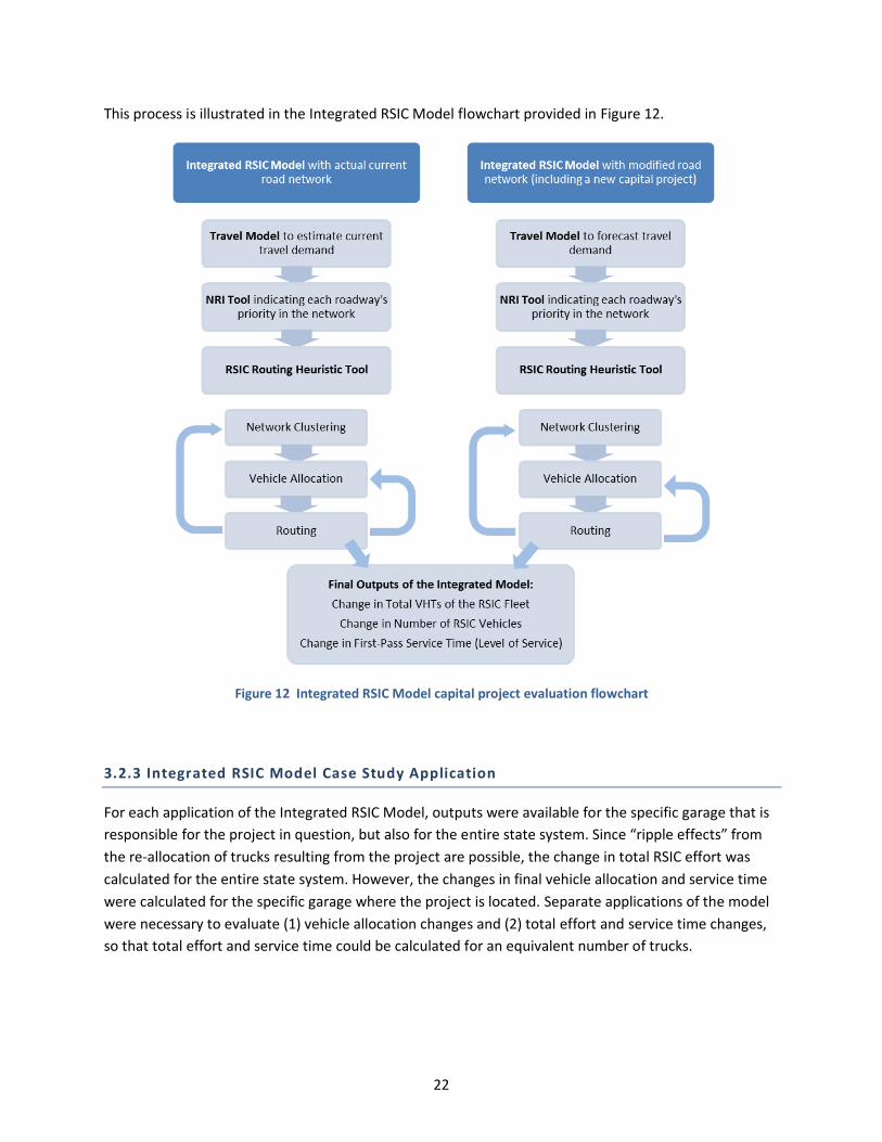
This process is illustrated in the Integrated RSIC Model flowchart provided in Figure 12.
Figure 12 Integrated RSIC Model capital project evaluation flowchart
3.2.3 Integrated RSIC Model Case Study Application
For each application of the Integrated RSIC Model, outputs were available for the specific garage that is
responsible for the project in question, but also for the entire state system. Since “ripple effects” from
the re-allocation of trucks resulting from the project are possible, the change in total RSIC effort was
calculated for the entire state system. However, the changes in final vehicle allocation and service time
were calculated for the specific garage where the project is located. Separate applications of the model
were necessary to evaluate (1) vehicle allocation changes and (2) total effort and service time changes,
so that total effort and service time could be calculated for an equivalent number of trucks.

23
Table 4 provides a summary of the application scenarios of the Integrated RSIC Model that were
necessary for this project.
Table 4 Integrated RSIC Model application scenarios
Allocation Method /
Storm-Intensity
Combination
Full
(Baseline)
Network
Project Being Evaluated
Champlain
Parkway,
ChPa
Crescent
Connector,
CrCo
US Route 2
Left-Turn
Lanes,
Rt2Lefts
State Route
100 Lane
Addition,
Rt100Lane
Adds
Bennington
ByPass,
Southern
Segment,
BennBP
Miles Low-Salt
Storm X X X X X X
Miles High-Salt
Storm X X X X X X
NRI Low-Salt
Storm X X X X X X
NRI High-Salt
Storm X X X X X X
Any scenario which results in a different vehicle allocation between the Full (Baseline) Network and the
project being evaluated will also require a second application of the Integrated RSIC Model with the
vehicle allocations matched in order to make a valid comparison of RSIC effort. Therefore, between 24
and 48 applications of the Integrated RSIC Model were conducted. Each run of the Model requires 2-3
hours of processing time, for a project total of between 48 and 144 hours of runtime.
3.3 CALCULATION TOOL DEVELOPMENT
The outputs of the Integrated RSIC Model applications were used to populate a calculation tool for
practitioners to make estimates of the RSIC burden increase from a variety of common project types.
From the outputs of the Integrated RSIC Model runs, the team developed an Excel-based decision-
support tool to allow users to enter their own specific monetary costs for fuel, salt, labor, and vehicle
operation and get an estimated cost for the impact of each type of capital improvement investigated.
The tool is intended to be used by operations planners and supervisors to justify budget requests in
advance of a new capital project.
MS Excel provides a user-friendly computational platform for automating calculations summarizing the
impact of capital improvements on RSIC burden. Spreadsheet-based decision-support tools built in Excel
allow users to examine scenarios, change inputs, and view numeric and visual summaries in real-time.

24
This tool will be useful in estimating how new capital projects will create a need for additional RSIC
budgetary resources. The tool was created as an extension of Excel using Visual Basic for Applications
(VBA), the programming language for Excel. With VBA, a user-friendly interface can be built in the
familiar spreadsheet environment. When the user is not likely to be interested in the mathematical form
of the underlying model parameters, only in its application to a specific decision task, this type of
extension is perfectly suited. The familiar spreadsheet interface gives users total access to the model’s
functionality via simple inputs and provides results as nontechnical outputs. The outputs of the
Integrated RSIC Model application in Vermont were converted into unit rates for measuring RSIC burden
increase, in units of (1) vehicle-minutes of effort, (2) new RSIC vehicles, and (3) loss of service time.
These rates make the Excel tool generalizable to all of the Clear Roads’ member states.
25
RESULTS
4.1 INCREASED RSIC BURDEN FOR THE ROUNDABOUT IN LANCASTER, NEW HAMPSHIRE
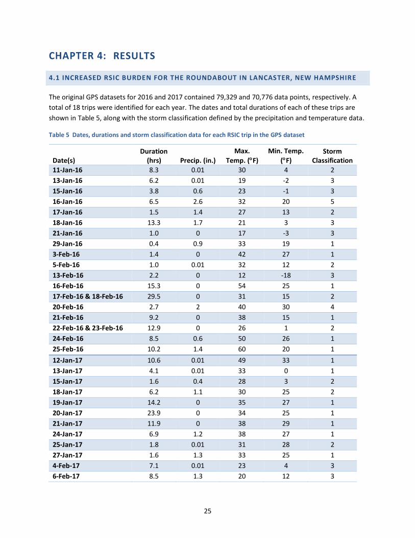
The original GPS datasets for 2016 and 2017 contained 79,329 and 70,776 data points, respectively. A
total of 18 trips were identified for each year. The dates and total durations of each of these trips are
shown in Table 5, along with the storm classification defined by the precipitation and temperature data.
Table 5 Dates, durations and storm classification data for each RSIC trip in the GPS dataset
Date(s) Duration
(hrs) Precip. (in.)
Max.
Temp. (F)
Min. Temp.
(F) Storm
Classification
11-Jan-16 8.3 0.01 30 4 2
13-Jan-16 6.2 0.01 19 -2 3
15-Jan-16 3.8 0.6 23 -1 3
16-Jan-16 6.5 2.6 32 20 5
17-Jan-16 1.5 1.4 27 13 2
18-Jan-16 13.3 1.7 21 3 3
21-Jan-16 1.0 0 17 -3 3
29-Jan-16 0.4 0.9 33 19 1
3-Feb-16 1.4 0 42 27 1
5-Feb-16 1.0 0.01 32 12 2
13-Feb-16 2.2 0 12 -18 3
16-Feb-16 15.3 0 54 25 1
17-Feb-16 & 18-Feb-16 29.5 0 31 15 2
20-Feb-16 2.7 2 40 30 4
21-Feb-16 9.2 0 38 15 1
22-Feb-16 & 23-Feb-16 12.9 0 26 1 2
24-Feb-16 8.5 0.6 50 26 1
25-Feb-16 10.2 1.4 60 20 1
12-Jan-17 10.6 0.01 49 33 1
13-Jan-17 4.1 0.01 33 0 1
15-Jan-17 1.6 0.4 28 3 2
18-Jan-17 6.2 1.1 30 25 2
19-Jan-17 14.2 0 35 27 1
20-Jan-17 23.9 0 34 25 1
21-Jan-17 11.9 0 38 29 1
24-Jan-17 6.9 1.2 38 27 1
25-Jan-17 1.8 0.01 31 28 2
27-Jan-17 1.6 1.3 33 25 1
4-Feb-17 7.1 0.01 23 4 3
6-Feb-17 8.5 1.3 20 12 3

26
Date(s) Duration
(hrs) Precip. (in.)
Max.
Temp. (F)
Min. Temp.
(F) Storm
Classification
7-Feb-17 & 8-Feb-17 28.0 2.7 29 13 5
9-Feb-17 4.9 1.8 17 -6 3
14-Feb-17 1.7 0.7 28 6 2
15-Feb-17 9.8 2.8 26 19 5
16-Feb-17 1.6 0.01 27 -2 2
7-Mar-17 8.0 0 55 38 1
Given the routing differences between years for these trips, a buffer was used to extract only data
points within a 1-km radius of the intersection being converted to a roundabout between 2016 and
2017. Figure 13a and 13b show the data points within the 1 km buffer of the intersection for 2015-2016
and 2016-2017, respectively.
a

27
Figure 13 GPS data points within the 1 km buffer of the intersection for 2015-2016 (a) and 2016-2017 (b)
98 trip segments were created for 2016 and 108 trip segments were created for 2017, indicating that
the average number of passes for each season were 5.5 and 6.0, respectively. Table 6 summarizes and
compares the average time taken to make a RSIC service pass and the average speed of the service, as
calculated from trip segments grouped by specific winter storm category.
Table 6 Average time and average speed of RSIC service by storm class
Year # of Trip Segments Storm Class Avg. Time (min.) Avg. Speed (kph)
2016 27 1 3.82 36.2
2016 17 2 3.26 37.8
2016 36 3 4.23 31.9
2016 6 4 3.02 36.8
2016 12 5 4.14 32.0
b

28
Year # of Trip Segments Storm Class Avg. Time (min.) Avg. Speed (kph)
2017 37 1 3.72 35.9
2017 21 2 5.03 31.2
2017 25 3 3.34 36.8
2017 0 4 - -
2017 25 5 4.28 32.2
The same set of outputs for the aggregated classes, representing a storm that would not be likely to
require a high amount of salt (classes 1 and 3 – low-salt) and a storm that would (classes 2, 4, and 5 –
high-salt), are shown in Table 7, although now the aggregate average time to service the project area is
also provided, - representing the average time multiplied by the average number of passes.
Table 7 Average time and average speed of RSIC service by storm severity
Year # of Trip
Segments Storm
Severity Avg. Speed
(kph) Avg. Time
(min.)
Average Number of
Passes
Aggregate Avg. Time
(min.)
2016 63 LS 33.7 4.06 5.5 22.3
2016 35 HS 35.6 3.52 5.5 19.4
2017 62 LS 36.2 3.56 6.0 21.4
2017 46 HS 31.7 4.62 6.0 27.7
As seen in the table, the introduction of the roundabout had mixed effects on RSIC burden. It resulted in
a decrease in average speed and an increase in the number of passes needed for the high-salt snow
events. This finding is consistent with what was expected by field reports from drivers and supervisors.
However, the effect was reversed for low-salt storms, where the roundabout increased the RSIC speed
slightly. The result was an increase in RSIC effort of 8.3 minutes for the high-salt storm, and a decrease
of 0.9 minutes for the low-salt storm.
The reason for this finding could be related to the fact that cars are also present in the roundabout, and
will have an effect on the speed and effectiveness of the RSIC service. The absence of cars in the
roundabout will allow the RSIC vehicle to proceed through more quickly, but congestion or stopped
vehicles in the roundabout will cause the service to take longer. Overall, though, the findings were
consistent with expectations, with a net slowing effect of the roundabout on RSIC service.
4.2 INCREASED RSIC BURDEN FOR THE CHAMPLAIN PARKWAY IN BURLINGTON, VERMONT
The RSIC burden created by the proposed construction of the Champlain Parkway in Burlington (Figure
11) was measured as the difference in the final allocation to the garage responsible for this roadway
(the Colchester garage), then also as the increase in service time created by the project in the Colchester
garage or elsewhere in the state, and finally also as the increase in total effort, as measured by
statewide vehicle-minutes of travel per pass. The results of the Integrated RSIC Model applications
conducted for this project are provided in Table 8.

29
Table 8 Results of Integrated RSIC Model applications for the Champlain Parkway project
Allocation
Method Scenario
Storm
Severity
Final
Allocation
District
Service Time
(min.)
Statewide
Service Time
(min.)
Total Effort
(vehicle-
minutes)
Miles
Without
Low Salt
9 123 133 15,289
With 9 132 133 15,471
With 11 NA
Without
High Salt
9 130 133 15,402
With 9 130 133 15,813
With 10 NA
NRI
Without Low Salt
16 113 133 15,613
With 17 NA
Without High Salt
16 103 128 15,601
With 17 NA
As shown in the table, the application of the Integrated RSIC Model with the project in place resulted in
an increased vehicle allocation for its garage in all four allocation method / storm severity combinations.
For the low-salt storm scenarios, the average allocation increase was 1.5 trucks (11–9 & 17–16),
whereas the increases for the high-salt storm scenarios were both 1.0 trucks (10–9 & 17–16). To
calculate the increased total effort from the project, the scenarios with identical vehicle allocations were
compared. For the low-salt scenario, the project resulted in an additional 182 (15,471 – 15,289) vehicle-
minutes of travel per pass. For the high-salt scenario, the project resulted in an additional 411 vehicle-
minutes of travel per pass. To find the increased service time from the project, the largest of the
increases for the entire state and for the specific garage where the project is located was calculated. For
the low-salt scenarios, the highest service-time increase was 9 minutes (132 – 123). For the high-salt
scenarios, the highest service-time increase was 0 minutes.
30
4.3 INCREASED RSIC BURDEN FOR THE CRESCENT CONNECTOR IN ESSEX JUNCTION,
VERMONT
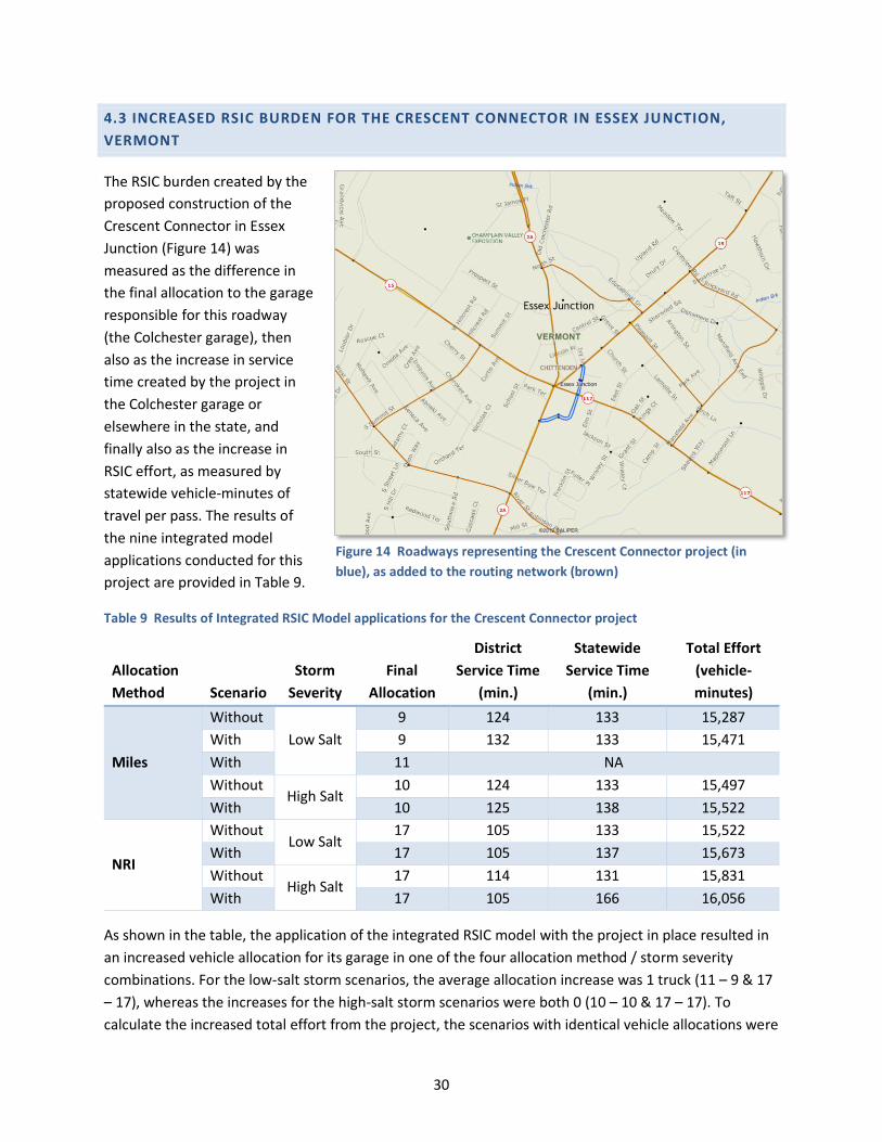
The RSIC burden created by the
proposed construction of the
Crescent Connector in Essex
Junction (Figure 14) was
measured as the difference in
the final allocation to the garage
responsible for this roadway
(the Colchester garage), then
also as the increase in service
time created by the project in
the Colchester garage or
elsewhere in the state, and
finally also as the increase in
RSIC effort, as measured by
statewide vehicle-minutes of
travel per pass. The results of
the nine integrated model
applications conducted for this
project are provided in Table 9.
Table 9 Results of Integrated RSIC Model applications for the Crescent Connector project
Allocation
Method Scenario
Storm
Severity
Final
Allocation
District
Service Time
(min.)
Statewide
Service Time
(min.)
Total Effort
(vehicle-
minutes)
Miles
Without
Low Salt
9 124 133 15,287
With 9 132 133 15,471
With 11 NA
Without High Salt
10 124 133 15,497
With 10 125 138 15,522
NRI
Without Low Salt
17 105 133 15,522
With 17 105 137 15,673
Without High Salt
17 114 131 15,831
With 17 105 166 16,056
As shown in the table, the application of the integrated RSIC model with the project in place resulted in
an increased vehicle allocation for its garage in one of the four allocation method / storm severity
combinations. For the low-salt storm scenarios, the average allocation increase was 1 truck (11 – 9 & 17
– 17), whereas the increases for the high-salt storm scenarios were both 0 (10 – 10 & 17 – 17). To
calculate the increased total effort from the project, the scenarios with identical vehicle allocations were
Figure 14 Roadways representing the Crescent Connector project (in
blue), as added to the routing network (brown)
31
compared. For the low-salt scenarios, the project resulted in an additional average of 168 (15,471 –
15,287 & 15,673 – 15,522) vehicle-minutes of travel per pass, whereas the corresponding increase for
the high-salt storm scenario averaged 125 vehicle-minutes of travel per pass. For the low-salt scenarios,
the highest service-time increase was 8 minutes (132 – 124). For the high-salt scenarios, the highest
service-time increase was 35 minutes (166 – 131).
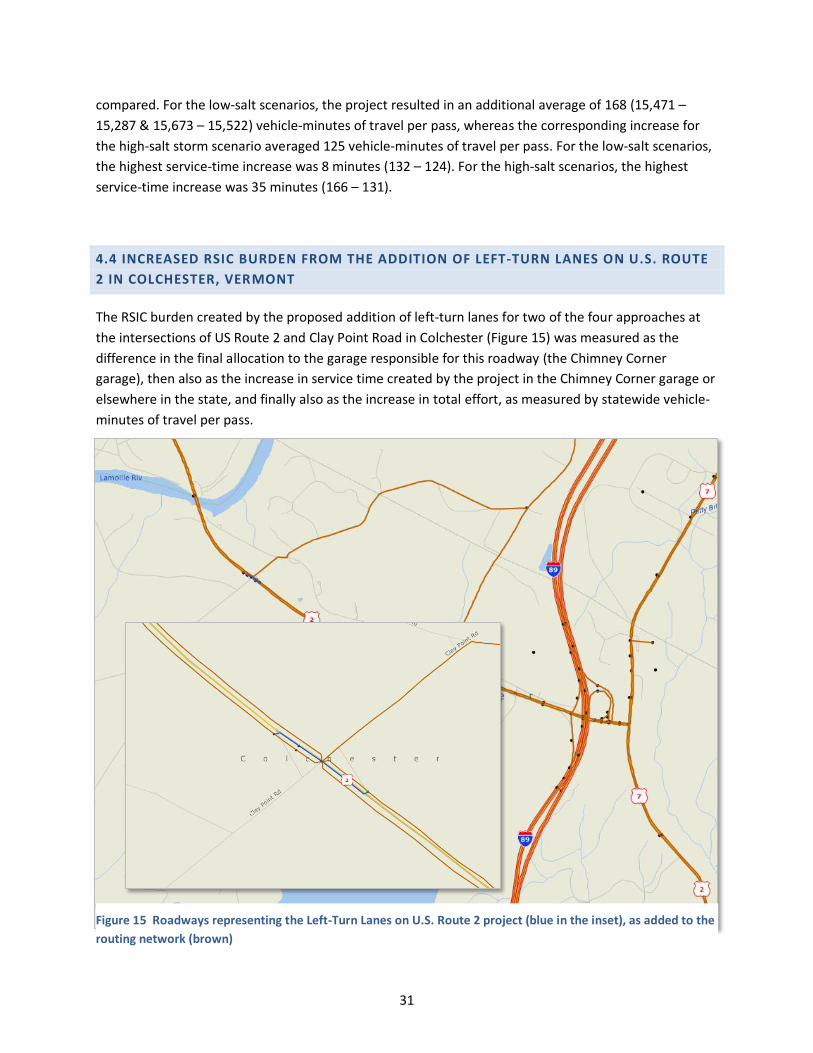
4.4 INCREASED RSIC BURDEN FROM THE ADDITION OF LEFT-TURN LANES ON U.S. ROUTE
2 IN COLCHESTER, VERMONT
The RSIC burden created by the proposed addition of left-turn lanes for two of the four approaches at
the intersections of US Route 2 and Clay Point Road in Colchester (Figure 15) was measured as the
difference in the final allocation to the garage responsible for this roadway (the Chimney Corner
garage), then also as the increase in service time created by the project in the Chimney Corner garage or
elsewhere in the state, and finally also as the increase in total effort, as measured by statewide vehicle-
minutes of travel per pass.
Figure 15 Roadways representing the Left-Turn Lanes on U.S. Route 2 project (blue in the inset), as added to the
routing network (brown)

32
The results of the eight integrated model applications conducted for this project are provided in Table
10.
Table 10 Results of Integrated RSIC Model applications for the U.S Route 2 Left-Turn Lanes project
Allocation
Method Scenario
Storm
Severity
Final
Allocation
District
Service Time
(min.)
Statewide
Service Time
(min.)
Total Effort
(vehicle-
minutes)
Miles
Without Low Salt
3 68 133 15,234
With 3 82 133 15,479
Without High Salt
3 85 138 15,522
With 3 83 133 15,770
NRI
Without Low Salt
4 91 137 15,673
With 5 NA
Without High Salt
4 91 166 16,056
With 5 NA
As shown in the table, the application of the integrated RSIC model with the project in place resulted in
an increased vehicle allocation for its garage in two of the four allocation method/storm severity
combinations. For the low-salt storm scenarios, the average allocation increase was 0.5 trucks, whereas
the increases for the high-salt storm scenarios were both 0.5 trucks. To calculate the increased total
effort from the project, the two scenarios with identical vehicle allocations were compared. For the low-
salt scenarios, the project resulted in an additional 245 vehicle-minutes of travel per pass, whereas the
corresponding increase for the high-salt storm scenario was 248 vehicle-minutes of travel per pass. To
find the increased service time from the project, the largest of the increases for the entire state and for
the specific garage where the project is located was calculated. For the low-salt scenarios, the highest
service-time increase was 14 minutes. For the high-salt scenarios, the highest service-time increase was
0 minutes.

33
4.5 INCREASED RSIC BURDEN FROM THE ADDITION OF A LANE IN EACH DIRECTION OF
STATE ROUTE 100 IN WATERBURY, VERMONT
The RSIC burden created by the envisioned addition of one lane of travel in each direction of State Route
100 in Waterbury (Figure 16) was measured as the difference in the final allocation to the garage
responsible for this roadway (the Middlesex garage), then also as the increase in service time created by
the project, and finally also as the increase in total effort, as measured by statewide vehicle-minutes of
travel per pass.
Figure 16 Roadways representing the Addition of a Lane in Each Direction on U.S. Route 100 project (in blue), as
added to the routing network (brown)
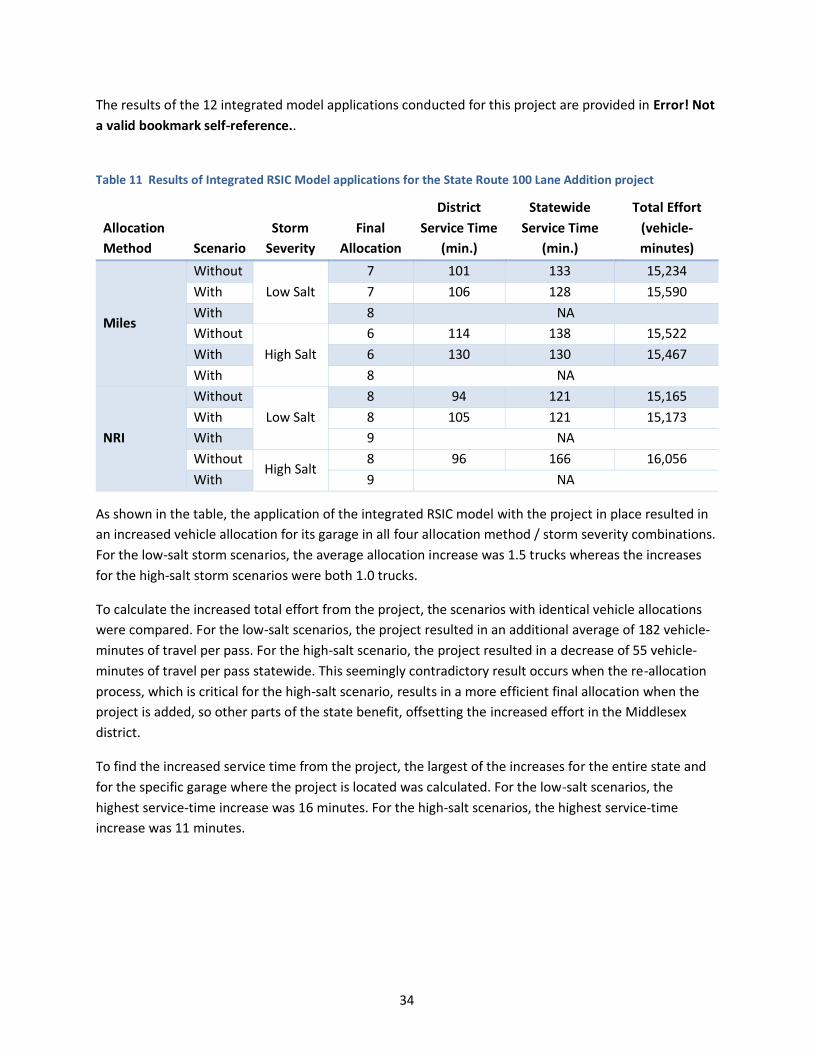
34
The results of the 12 integrated model applications conducted for this project are provided in Error! Not
a valid bookmark self-reference..
Table 11 Results of Integrated RSIC Model applications for the State Route 100 Lane Addition project
Allocation
Method Scenario
Storm
Severity
Final
Allocation
District
Service Time
(min.)
Statewide
Service Time
(min.)
Total Effort
(vehicle-
minutes)
Miles
Without
Low Salt
7 101 133 15,234
With 7 106 128 15,590
With 8 NA
Without
High Salt
6 114 138 15,522
With 6 130 130 15,467
With 8 NA
NRI
Without
Low Salt
8 94 121 15,165
With 8 105 121 15,173
With 9 NA
Without High Salt
8 96 166 16,056
With 9 NA
As shown in the table, the application of the integrated RSIC model with the project in place resulted in
an increased vehicle allocation for its garage in all four allocation method / storm severity combinations.
For the low-salt storm scenarios, the average allocation increase was 1.5 trucks whereas the increases
for the high-salt storm scenarios were both 1.0 trucks.
To calculate the increased total effort from the project, the scenarios with identical vehicle allocations
were compared. For the low-salt scenarios, the project resulted in an additional average of 182 vehicle-
minutes of travel per pass. For the high-salt scenario, the project resulted in a decrease of 55 vehicle-
minutes of travel per pass statewide. This seemingly contradictory result occurs when the re-allocation
process, which is critical for the high-salt scenario, results in a more efficient final allocation when the
project is added, so other parts of the state benefit, offsetting the increased effort in the Middlesex
district.
To find the increased service time from the project, the largest of the increases for the entire state and
for the specific garage where the project is located was calculated. For the low-salt scenarios, the
highest service-time increase was 16 minutes. For the high-salt scenarios, the highest service-time
increase was 11 minutes.
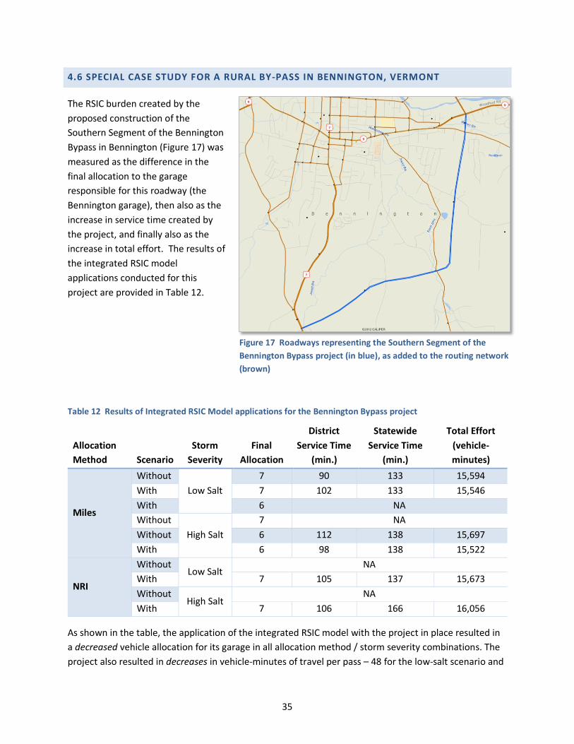
35
4.6 SPECIAL CASE STUDY FOR A RURAL BY-PASS IN BENNINGTON, VERMONT
The RSIC burden created by the
proposed construction of the
Southern Segment of the Bennington
Bypass in Bennington (Figure 17) was
measured as the difference in the
final allocation to the garage
responsible for this roadway (the
Bennington garage), then also as the
increase in service time created by
the project, and finally also as the
increase in total effort. The results of
the integrated RSIC model
applications conducted for this
project are provided in Table 12.
Table 12 Results of Integrated RSIC Model applications for the Bennington Bypass project
Allocation
Method Scenario
Storm
Severity
Final
Allocation
District
Service Time
(min.)
Statewide
Service Time
(min.)
Total Effort
(vehicle-
minutes)
Miles
Without
Low Salt
7 90 133 15,594
With 7 102 133 15,546
With 6 NA
Without
High Salt
7 NA
Without 6 112 138 15,697
With 6 98 138 15,522
NRI
Without Low Salt
NA
With 7 105 137 15,673
Without High Salt
NA
With 7 106 166 16,056
As shown in the table, the application of the integrated RSIC model with the project in place resulted in
a decreased vehicle allocation for its garage in all allocation method / storm severity combinations. The
project also resulted in decreases in vehicle-minutes of travel per pass – 48 for the low-salt scenario and
Figure 17 Roadways representing the Southern Segment of the
Bennington Bypass project (in blue), as added to the routing network
(brown)

36
175 for the high-salt scenario. For the low-salt scenario, the highest service-time increase was 12
minutes. For the high-salt scenario, the highest service-time increase was 0 minutes.
The rural bypass is a special case study that makes it unique among the other case studies because the
RSIC burden actually diminished when a new road was added to the network, which is why the
applications using the NRI allocation method were not completed. This decrease is created because the
new roadway creates a shortcut from the edge of a route to the edge of another route that previously
required “deadheading”, or traversing links without providing RSIC service. Deadheading occurs when a
roadway is traversed without providing service, either because it has already been provided by another
route or because the roadway is not part of the state-maintained network.
So the new bypass create a shortcut for snow and ice control vehicles to bypass roads that are not part
of the state-maintained network (in green in Figure 18) in the same way that it creates a shortcut for
vehicles bypassing the downtown.

37
In this unique situation, additional resources are not required by the district where the rural bypass had
been constructed, even though the roadway mileage it is responsible for has increased. However, this
conclusion is only applicable to the specific network structure created by a rural state-maintained
bypass around a small micropolitan “crossroads” community whose downtown roads are not the
responsibility of the state agency. RSIC vehicles approach the small micropolitan community, stop
servicing the roadway at a certain point and then drive through the downtown without providing
service, then out of the small micropolitan community to the continuation of the RSIC route where the
state-maintained roadway begins again. The new bypass creates a shortcut that makes the deadheading
in the downtown community unnecessary and reduces the distance traveled.
Figure 18 Roads that are not part of the state-maintained network (in green) are bypassed by the new project
(in blue)

38
4.7 SUMMARY OF RESULTS FOR USE IN THE CALCULATION TOOL
Table 13 contains a summary of the results of the Integrated RSIC Model applications for the increase in
effort measured as increase in the total vehicle-minutes of travel for each pass.
Table 13 Summary of results of the Integrated RSIC Model applications for increased RSIC effort
Project
ID Project Type Quantity Unit
Region
Type
Low-Salt
Storm
High-Salt
Storm
Average Unit
Increase (min.)
CrCo New roadway, 1-lane
either direction 0.55 miles suburban 168 125 266 per mi.
ChPa New roadway, 1-lane
either direction 3.56 miles urban 182 411 83 per mi.
Rt2Lefts New left-turn lanes,
2 of 4 approaches 2 approach rural 245 248 123
per
approach
BennBP New roadway, 1-lane
either direction 3.26 miles rural -48 -175 -34 per mi.
Rt100La
neAdds
Highway lane
addition, from 1 to 2
in both directions
9.20 miles rural 356 63 23 per mi.
NH
Round-
about
Conversion of stop-
and yield-controlled
intersection to a
roundabout
1 each rural -1 8 4 per intx
For each of these applications, the number of vehicles was held fixed, so the results assume that no new
vehicles (trucks or tow-plows) are added to the RSIC fleet. The effects of the new suburban roadway
(CrCo) were the most significant, as expected since the road network is less connected outside of the
urban core and there are fewer opportunities to devise an alternative set of efficient routes with the
new roadway. In an urban core, adding a new roadway (ChPa) has less of an effect on RSIC effort
because it is more likely that an existing route can be extended to cover it without the addition of much
deadheading. Note also the negative effects of the addition of a bypass system for a new roadway in a
rural micropolitan community.
Adding left-turn lanes to a rural intersection approach (Rt2Lefts) also had a significant effect on RSIC
effort. These types of intersection improvements are common in rural and suburban areas where right-
of-way is available for the addition of turning lanes, but their considerable effect on RSIC effort must be
considered, especially in relation to the more moderate effect of converting a rural intersection to a
roundabout. The impact of adding left-turn lanes might be moderated if the intersection being
considered consists of four approaches that are all state-maintained roadways. However, in this case, as
is true of many rural intersections, the major roadway is state-maintained, but the minor roadway is not,
so only two of the four approaches are being modified and the state’s responsibility is only for those two
approaches, so a significant amount of deadheading is involved with getting both lanes plowed.
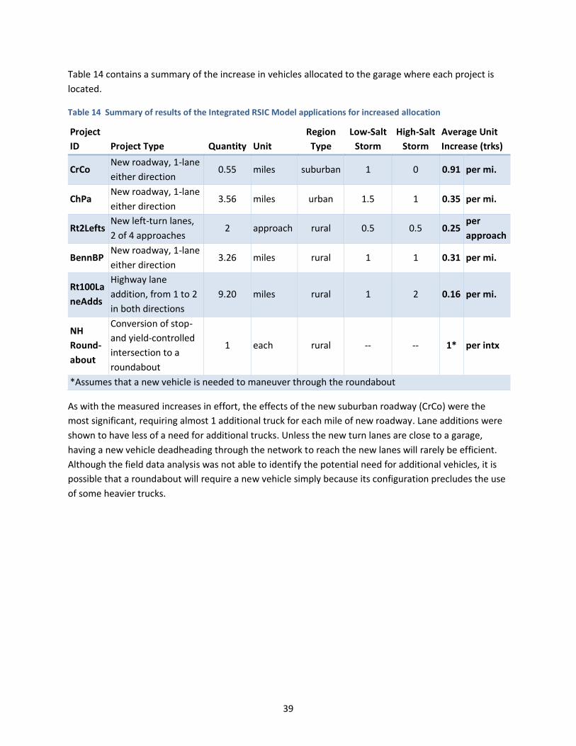
39
Table 14 contains a summary of the increase in vehicles allocated to the garage where each project is
located.
Table 14 Summary of results of the Integrated RSIC Model applications for increased allocation
Project
ID Project Type Quantity Unit
Region
Type
Low-Salt
Storm
High-Salt
Storm
Average Unit
Increase (trks)
CrCo New roadway, 1-lane
either direction 0.55 miles suburban 1 0 0.91 per mi.
ChPa New roadway, 1-lane
either direction 3.56 miles urban 1.5 1 0.35 per mi.
Rt2Lefts New left-turn lanes,
2 of 4 approaches 2 approach rural 0.5 0.5 0.25
per
approach
BennBP New roadway, 1-lane
either direction 3.26 miles rural 1 1 0.31 per mi.
Rt100La
neAdds
Highway lane
addition, from 1 to 2
in both directions
9.20 miles rural 1 2 0.16 per mi.
NH
Round-
about
Conversion of stop-
and yield-controlled
intersection to a
roundabout
1 each rural -- -- 1* per intx
*Assumes that a new vehicle is needed to maneuver through the roundabout
As with the measured increases in effort, the effects of the new suburban roadway (CrCo) were the
most significant, requiring almost 1 additional truck for each mile of new roadway. Lane additions were
shown to have less of a need for additional trucks. Unless the new turn lanes are close to a garage,
having a new vehicle deadheading through the network to reach the new lanes will rarely be efficient.
Although the field data analysis was not able to identify the potential need for additional vehicles, it is
possible that a roundabout will require a new vehicle simply because its configuration precludes the use
of some heavier trucks.
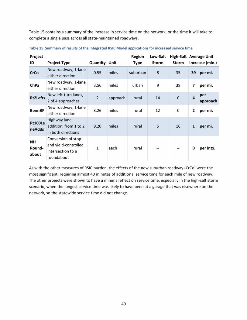
40
Table 15 contains a summary of the increase in service time on the network, or the time it will take to
complete a single pass across all state-maintained roadways.
Table 15 Summary of results of the Integrated RSIC Model applications for increased service time
Project
ID Project Type Quantity Unit
Region
Type
Low-Salt
Storm
High-Salt
Storm
Average Unit
Increase (min.)
CrCo New roadway, 1-lane
either direction 0.55 miles suburban 8 35 39 per mi.
ChPa New roadway, 1-lane
either direction 3.56 miles urban 9 38 7 per mi.
Rt2Lefts New left-turn lanes,
2 of 4 approaches 2 approach rural 14 0 4
per
approach
BennBP New roadway, 1-lane
either direction 3.26 miles rural 12 0 2 per mi.
Rt100La
neAdds
Highway lane
addition, from 1 to 2
in both directions
9.20 miles rural 5 16 1 per mi.
NH
Round-
about
Conversion of stop-
and yield-controlled
intersection to a
roundabout
1 each rural -- -- 0 per intx.
As with the other measures of RSIC burden, the effects of the new suburban roadway (CrCo) were the
most significant, requiring almost 40 minutes of additional service time for each mile of new roadway.
The other projects were shown to have a minimal effect on service time, especially in the high-salt storm
scenario, when the longest service time was likely to have been at a garage that was elsewhere on the
network, so the statewide service time did not change.
41
CONCLUSIONS AND RECOMMENDATIONS
The results and findings of this research have implications for short-term funding allocations for RSIC
operations staff and for long-term consideration of RSIC in the highway planning and design processes.
The findings of this project provide defensible data for operations staff to advocate for increases in
funding to offset the increased RSIC burden when a project is completed. The calculation tool described
in Chapter 3.3 incorporates all of the results summarized in Chapter 4.7 into a MS Excel decision support
platform, providing quick estimates of the monetary impact of a variety of major highway project types
(Figure 19).
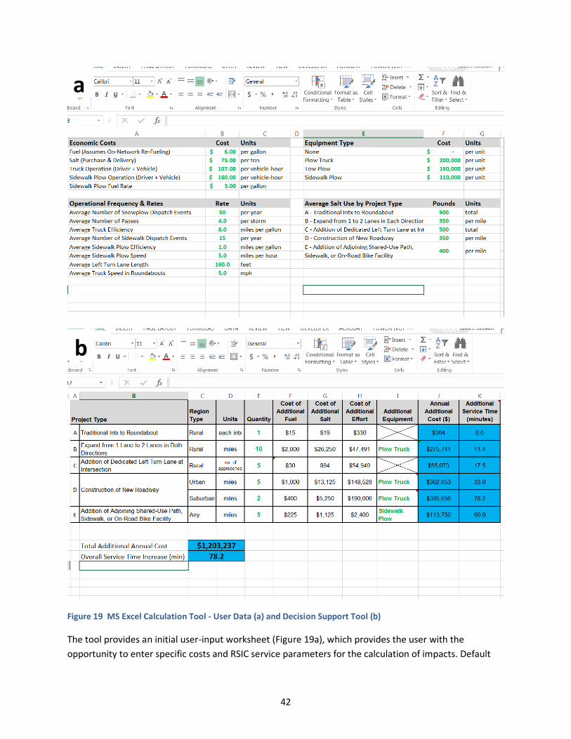
42
Figure 19 MS Excel Calculation Tool - User Data (a) and Decision Support Tool (b)
The tool provides an initial user-input worksheet (Figure 19a), which provides the user with the
opportunity to enter specific costs and RSIC service parameters for the calculation of impacts. Default
a
b
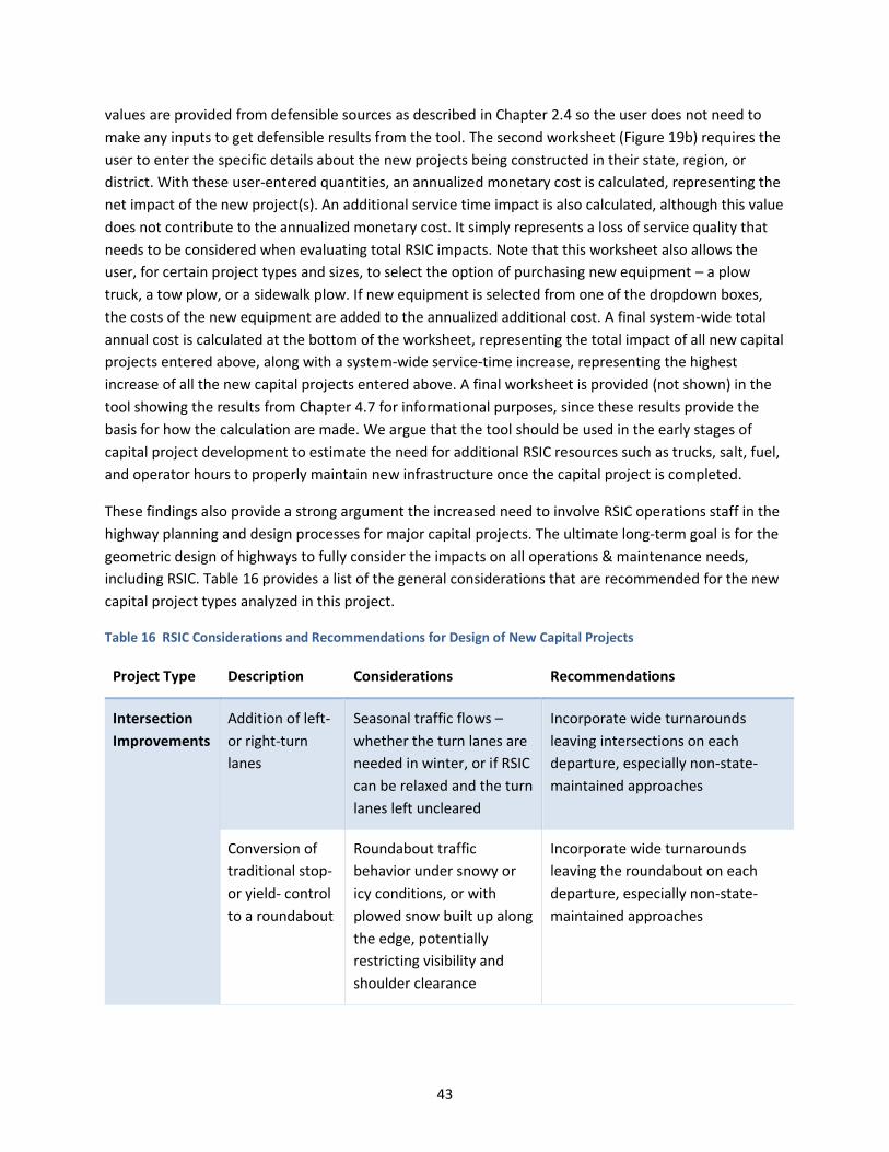
43
values are provided from defensible sources as described in Chapter 2.4 so the user does not need to
make any inputs to get defensible results from the tool. The second worksheet (Figure 19b) requires the
user to enter the specific details about the new projects being constructed in their state, region, or
district. With these user-entered quantities, an annualized monetary cost is calculated, representing the
net impact of the new project(s). An additional service time impact is also calculated, although this value
does not contribute to the annualized monetary cost. It simply represents a loss of service quality that
needs to be considered when evaluating total RSIC impacts. Note that this worksheet also allows the
user, for certain project types and sizes, to select the option of purchasing new equipment – a plow
truck, a tow plow, or a sidewalk plow. If new equipment is selected from one of the dropdown boxes,
the costs of the new equipment are added to the annualized additional cost. A final system-wide total
annual cost is calculated at the bottom of the worksheet, representing the total impact of all new capital
projects entered above, along with a system-wide service-time increase, representing the highest
increase of all the new capital projects entered above. A final worksheet is provided (not shown) in the
tool showing the results from Chapter 4.7 for informational purposes, since these results provide the
basis for how the calculation are made. We argue that the tool should be used in the early stages of
capital project development to estimate the need for additional RSIC resources such as trucks, salt, fuel,
and operator hours to properly maintain new infrastructure once the capital project is completed.
These findings also provide a strong argument the increased need to involve RSIC operations staff in the
highway planning and design processes for major capital projects. The ultimate long-term goal is for the
geometric design of highways to fully consider the impacts on all operations & maintenance needs,
including RSIC. Table 16 provides a list of the general considerations that are recommended for the new
capital project types analyzed in this project.
Table 16 RSIC Considerations and Recommendations for Design of New Capital Projects
Project Type Description Considerations Recommendations
Intersection
Improvements
Addition of left-
or right-turn
lanes
Seasonal traffic flows –
whether the turn lanes are
needed in winter, or if RSIC
can be relaxed and the turn
lanes left uncleared
Incorporate wide turnarounds
leaving intersections on each
departure, especially non-state-
maintained approaches
Conversion of
traditional stop-
or yield- control
to a roundabout
Roundabout traffic
behavior under snowy or
icy conditions, or with
plowed snow built up along
the edge, potentially
restricting visibility and
shoulder clearance
Incorporate wide turnarounds
leaving the roundabout on each
departure, especially non-state-
maintained approaches

44
Project Type Description Considerations Recommendations
New roadway
construction
One lane each
direction
Connections to non-state-
maintained facilities
Network connectivity
effects for routing
Use wider lanes and shoulders
where winter traffic requires that
the roadway be kept clear
Design roadways with smooth
transitions from other state-
maintained facilities to facilitate
heavy vehicle movement around
turns
Reduce or eliminate the need for
deadheading when servicing state-
maintained facilities by ensuring
route connectivity, or provide
adequate turnarounds.
Roadway
expansion
One lane each
direction to two
lanes each
direction; two
lanes each
direction to
three lanes each
direction
Use wider lanes and shoulders
where winter traffic requires that
the roadway be kept clear
Reduce or eliminate the need for
deadheading when servicing state-
maintained facilities by ensuring
route connectivity, or provide
adequate turnarounds.
Avoid adding lanes to highways in
rural areas where network
connectivity is poor, or where
distance to the nearest district
garage is far
45
REFERENCES
Dowds, Jonathan, James L. Sullivan, David C. Novak, and Darren Scott, 2014. Strategic Location of
Satellite Salt Storage for Roadway Snow and Ice Control in Vermont. Prepared for the Vermont Agency
of Transportation Policy, Planning & Research Bureau by the UVM Transportation Research Center,
Report No. 14-016, July 2014.
Dowds, Jonathan, James L. Sullivan, David C. Novak, and Darren Scott, 2013. Optimization of Snow
Removal in Vermont. Prepared for the Vermont Agency of Transportation Materials & Research Section
by the UVM Transportation Research Center, Report No. 13-005, December 2013.
Nixon, Wilfrid A., and Lin Qiu, 2005. Developing a Storm Severity Index. Transportation Research Record:
Journal of the Transportation Research Board, No. 1911, Transportation Research Board of the National
Academies, Washington, D.C., 2005, pp. 143–148.
Novak, D.C. and James L. Sullivan, 2014. A Link-Focused Methodology for Evaluating Accessibility to
Emergency Services. Decision Support Systems, Volume 57 (January 2014): 309-319.
Novak, David C., James L. Sullivan, and Darren M. Scott, 2012. A Network-Based Approach for Evaluating
and Ranking Transportation Roadway Projects. Applied Geography, Volume 34 (May 2012): 498–506.
Sullivan, James L., David C. Novak, Lisa Aultman-Hall and Darren Scott, 2010. Identifying Critical Road
Segments and Measuring System-Wide Robustness in Transportation Networks with Isolating Links: A
Link-Based Capacity-Reduction Approach. Transportation Research Part A, Volume 44 (2010): 323–336.
Sullivan, James, and Matt Conger, 2013. Vermont Travel Model 2012-2013 (Year 5) Report. Prepared for
the Vermont Agency of Transportation Policy & Planning Section by the UVM Transportation Research
Center, Report No. 13-015, December 2013.
Sullivan, James, David C. Novak, and Darren Scott, 2013. Travel Importance and Strategic Investment in
Vermont’s Transportation Assets. Prepared for the Vermont Agency of Transportation Materials &
Research Section by the UVM Transportation Research Center, Report No. 13-016, December 2013.
Sustainable Streets: Sidewalk Reference Manual. Onondaga County Sustainable Streets Project
Reference Document, June 2014. Accessed at http://walkbikecny.org/wp-
content/uploads/2014/06/SSM_ch6_Sidewalk_Finances.pdf on March 16, 2017.
Hossain, Kamal and Liping Fu, 2015. Optimal Snow and Ice Control of Parking Lots and
Sidewalks: A Summary Final Report. Prepared by the iTSS Lab, Department of Civil & Environmental
Engineering University of Waterloo, Ontario, Canada, January, 2015.

A-1
APPENDIX A
SURVEY RESPONSES
From: Peters, Thomas (DOT) [mailto:[email protected]]
Sent: Friday, August 28, 2015 8:15 AM
To: James Sullivan <[email protected]>
Subject: Re: [SNOW-ICE] Last call for Case Studies Needed for Snow and Ice Control Project
Jim,
MnDOT will participate and look to provide some good examples.
Tom Peters
Maintenance Research Engineer
________________________________________
From: Anderle, Phillip [mailto:[email protected]]
Sent: Monday, August 31, 2015 7:20 AM
To: Brooks, Jeffrey <[email protected]>
Cc: James Sullivan <[email protected]>
Subject: RE: [SNOW-ICE] Last call for Case Studies Needed for Snow and Ice Control Project
Can you give Jim the details?
From: Brooks, Jeffrey
Sent: Friday, August 28, 2015 3:10 PM
To: Anderle, Phillip
Subject: RE: [SNOW-ICE] Last call for Case Studies Needed for Snow and Ice Control Project
I cannot identify any projects that would include roundabouts, however, we have some major
construction taking place on US 31 corridor between I-465 and Westfield that will have a significant
impact to SIC. It would be a good candidate.
J.D. Brooks
Greenfield District Highway Maintenance Director
32 South Broadway
Greenfield, IN 46140
Office: (317) 467-3484
Cell: (765) 617-8735
Email: [email protected]

A-2
________________________________________
From: Robert Lannert [mailto:[email protected]]
Sent: Monday, August 31, 2015 4:04 PM
To: James Sullivan <[email protected]>
Subject: RE: [SNOW-ICE] Last call for Case Studies Needed for Snow and Ice Control Project
This is Bob Lannert, the inventor of the TowPLow and retired MoDot Engineer. I have now personally
worked in over 16 states.
I am not sure if these problems fit your study but these impact DOT operating costs in snow removal
costs. Some are old problems, some new:
1. Raised “snow plow-able” center and edge markers dramatically increase blade costs.
Carbide blades previously last up to 3 winters. Now, some only last one storm due to
carbide fracturing by dynamic impact upon so called plow-able markers.
2. There is a major difference in plowing rumble strips which have been formed into concrete
and rolled into asphalt vs. those which are rotomilled into the pavement. The first extrudes
material upward which then react with plow blades.
3. The construction of building additional lanes and a center wall by filling and obliterating the
median has caused the agency to plow all snow to the right which blocks traffic when
performed compared to plowing some left into the median and some right to right ditch.
This practice of using the median has caused not only the need to plow more lanes but
further complicated how the work was performed. Note some states have ruled that they
cannot plow against the median barrier and form a ramp. Designing taller walls and storage
on left side would help to allow some snow to go left.
4. There are some areas where lanes have been added and the cross section slopes
dramatically change. The problem is that all snow plows need to operate on consistent
pavement and not on two different plains. This has cause major blade wear and additional
costs to plowing.
5. Some design geometrics does not provide ANY discharge and storage areas for snow. This
causes discharged windrows of snow to be left across other lanes without any resolution.
These are just quick notes of what I have seen the last 10 years….
Bob Lannert
Technical Support Engineer
Snow King Technologies consultant to
Viking Cives Midwest
Cell 573-690-7600

research for winter highway maintenance
Lead state:Minnesota Department of Transportation
Research Services395 John Ireland Blvd.
St. Paul, MN 55155


