

QUASI-ONE-DIMENSIONAL SCRAMJET COMBUSTOR FLOW SOLVER USING THE
NUMERICAL PROPULSION SYSTEM SIMULATION
by
LONG VU
Presented to the Faculty of the Graduate School of
The University of Texas at Arlington in Partial Fulfillment
of the Requirements
for the Degree of
MASTER OF SCIENCE IN AEROSPACE ENGINEERING
THE UNIVERSITY OF TEXAS AT ARLINGTON
May 2018

ii
Copyright © by Long Vu 2018
All Rights Reserved

iii
Acknowledgements
I would like to thank my parents and my grandparents for their financial and
emotional support during my study. I would also like to thank my supervisor professor Dr.
Donald Wilson for his guidance and thesis committee members: Dr. Luca Maddalena and
Dr. Brian Dennis for their ideas and feedback on the research work.
I would like extend my thanks to Nandakumar Vijayakumar for his help and
suggestions.
I would also like to thank all my new friends I have made along the way: James
Phan, Peter Dao, Erin Doyle, Vinny Williams… for their help and support.
May 15, 2018
iv
Abstract
QUASI_ONE_DIMENSIONAL SCRAMJET COMBUSTOR FLOW SOLVER USING THE
NUMERICAL PROPULSION SYSTEM SIMULATION
Long Vu, MS
The University of Texas at Arlington, 2018
Supervising Professor: Donald R. Wilson
The flow field inside a scramjet engine combustor involves complex phenomena
such as fuel-air mixing, combustion chemistry, and flow separation. In order to determine
the properties of the flow along the length of the combustor, mass, momentum and
energy balance equations are solved simultaneously using a numerical method. While a
full three dimensional computational simulation gives detailed results with high order of
accuracy, it demands a great amount of time and computational resource. A low order
analysis produces a fast overall picture of the combustor operation which in turn provides
valuable information suitable for the preliminary design process. This research work aims
to describe the analysis process of the scramjet combustor in which a quasi-one-
dimensional, multi-species, reacting real gas model of the flow is developed to address
the limitations in previous researches. The Numerical Propulsion System Simulation
(NPSS), into which the NASA Chemical Equilibrium with Applications (CEA) code is
integrated, is utilized as the platform to perform the analysis. The analytical model is
validated by comparison with experimental data from previous researches. The results
obtained by this method are expected to shed some light on the advantages of using
detailed chemistry with lower order analysis to calculate scramjet engine performance.
v
Table of Contents
Acknowledgements .............................................................................................................iii
Abstract .............................................................................................................................. iv
List of Illustrations ............................................................................................................. viii
List of Tables ....................................................................................................................... x
Chapter 1 Introduction......................................................................................................... 1
1.1 Ramjet, Scramjet and Dual-mode Scramjet ............................................................. 1
Ramjet Engine ................................................................................................... 1
Scramjet Engine ................................................................................................ 2
Dual-mode Scramjet Engine ............................................................................. 3
1.2 Operation of Dual-mode Scramjet ............................................................................ 4
Dual-mode Scramjet Combustor ....................................................................... 4
Dual-mode Scramjet Isolator ............................................................................. 8
1.3 Development History ................................................................................................ 9
Chapter 2 Literature Survey .............................................................................................. 11
2.1 Theoretical Researches .......................................................................................... 11
Heiser and Pratt’s Approach ........................................................................... 11
Ram-Scram Transition and Flame/Shock-Train Interactions in a
Model Scramjet Experiment ..................................................................................... 12
Hyshot Program............................................................................................... 13
2.2 Experimental Researches ...................................................................................... 14
Free Piston Shock Tunnel Experiment at University of
Queensland – T4 Scramjet: ...................................................................................... 14
Hyshot 2 Scramjet Flight Experiment .............................................................. 15
Investigation of the Isolator Flow of Scramjet Engines ................................... 17
vi
Chapter 3 The Numerical Propulsion System Simulation (NPSS) ................................... 19
3.1 Introduction of NPSS .............................................................................................. 19
3.2 NPSS Simulation Environment ............................................................................... 21
3.3 NPSS Components ................................................................................................ 23
Architecture, code language and basic objects ............................................... 23
Thermodynamic packages .............................................................................. 25
Solver .............................................................................................................. 26
Chapter 4 Quasi-one-dimensional Scramjet Isolator and Combustor Model ................... 28
4.1 Assumptions ........................................................................................................... 28
4.2 Conservation Equations ......................................................................................... 28
Conservation of Mass ...................................................................................... 29
Conservation of Momentum ............................................................................ 29
Conservation of Energy ................................................................................... 29
4.3 Combustor Analytical Model ................................................................................... 30
Algebraic Manipulation Involving the Conservation Equations ....................... 30
Friction Coefficient ........................................................................................... 32
Wall Heat Loss ................................................................................................ 33
Mixing Efficiency Curve ................................................................................... 34
NPSS Calculation Procedure .......................................................................... 35
4.4 Isolator Analytical Model ......................................................................................... 39
Empirical Formula of Pressure Distribution ..................................................... 39
NPSS Calculation Procedure .......................................................................... 40
Chapter 5 Results ............................................................................................................. 41
5.1 Combustor Code Validation .................................................................................... 41
5.2 Isolator Code Validation ......................................................................................... 47

vii
Chapter 6 Conclusion ........................................................................................................ 51
6.1 Summary ................................................................................................................ 51
6.2 Future Work ............................................................................................................ 52
Appendix A 4th order Runge-Kutta Method ....................................................................... 53
Appendix B Code outline................................................................................................... 55
References ........................................................................................................................ 84
Biographical Information ................................................................................................... 87
viii
List of Illustrations
Figure 1-1 Ramjet engine [4]. ............................................................................................. 2
Figure 1-2 Scramjet engine [4]. ........................................................................................... 2
Figure 1-3 Dual-mode scramjet engine [3].......................................................................... 4
Figure 1-4 Typical changes in flow properties through the combustor in scramjet mode
[6]. ....................................................................................................................................... 5
Figure 1-5 Typical changes in flow properties through the combustor in transition
between ramjet and scramjet mode [6]. .............................................................................. 6
Figure 1-6 Typical changes in flow properties through the combustor in ramjet mode [6]. 7
Figure 1-7 Shock free isolator [7]. ....................................................................................... 8
Figure 1-8 Isolator with oblique shock train [7]. .................................................................. 9
Figure 1-9 Isolator with normal shock train [7]. ................................................................... 9
Figure 2-1 T4 scramjet inlet configuration [16]. ................................................................ 15
Figure 2-2 Hyshot flight profile [17]. .................................................................................. 16
Figure 2-3 Combustor instrumentation layout [17]. ........................................................... 17
Figure 2-4 Drawing of the hypersonic shock tunnel TH2 [18]. .......................................... 17
Figure 3-1 Hybrid Simulation: 3-Dimensional Low Pressure Subsystem Model Coupled to
a 0-Dimensional High Pressure Core Model [20]. ............................................................ 20
Figure 3-2 Illustration of the NPSS Multidisciplinary Framework [21]. .............................. 22
Figure 3-3 NPSS Object-Oriented Open Architecture [22]. .............................................. 24
Figure 3-4 NPSS Turbojet Model [25]. .............................................................................. 25
Figure 3-5 Basic NPSS Solver Operation [30]. ................................................................. 26
Figure 4-1 Schematic of elemental control volume for burner analysis [7]. ...................... 28
Figure 4-2 Discretization of the combustor. ...................................................................... 36
Figure 4-3 NPSS calculation procedure flow chart. .......................................................... 37

ix
Figure 5-1 T4 scramjet geometry [7]. ................................................................................ 41
Figure 5-2 Pressure distribution comparison for Case 1 – T4 experiment. ...................... 43
Figure 5-3 Pressure distribution comparison for Case 2 – T4 experiment. ...................... 43
Figure 5-4 Pressure distribution comparison for Case 3 – T4 experiment. ...................... 44
Figure 5-5 Schematic of Hyshot 2 scramjet geometry (dimensions are in millimeters) [17].
.......................................................................................................................................... 45
Figure 5-6 Hyshot 2 combustor section geometry [7]. ...................................................... 45
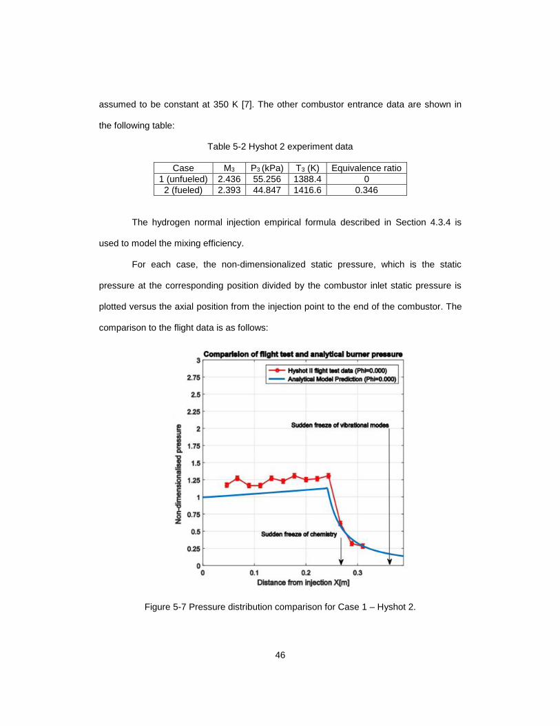
Figure 5-7 Pressure distribution comparison for Case 1 – Hyshot 2. ............................... 46
Figure 5-8 Pressure distribution comparison for Case 2 – Hyshot 2. ............................... 47
Figure 5-9 Heated isolator experiment setup [7]. .............................................................. 48
Figure 5-10 Pressure distribution comparison for the isolator – Fisher. ........................... 49
x
List of Tables
Table 5-1 T4 experiment data ........................................................................................... 42
Table 5-2 Hyshot 2 experiment data ................................................................................. 46
Table 5-3 Fisher experiment data ..................................................................................... 48
Table 5-4 Ma3 comparison – Fisher experiment .............................................................. 50

1
Chapter 1
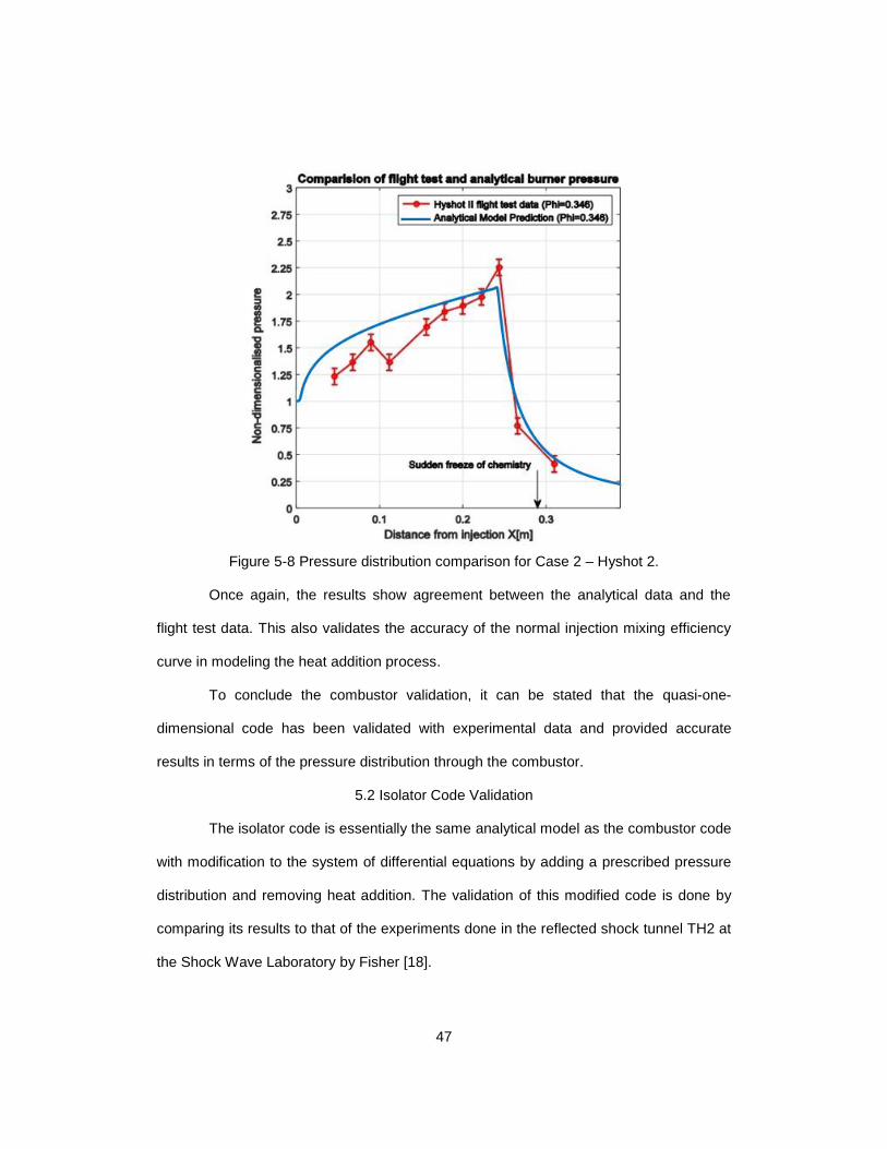
Introduction
Numerous programs aiming to develop aircraft capable of supersonic or
hypersonic flight first appeared in the late 1950’s and early 1960’s and have developed
unceasingly ever since [1]. Rocket propelled vehicles are not a practical option due to the
need of an onboard oxidizer tank, resulting in low specific impulse [2]. A more promising
choice for these high speed missions is an air breathing propulsion system and the best
suitable air breathing engine cycle for moderate supersonic flight is the ramjet, and for
hypersonic flight the scramjet or supersonic combustion ramjet, a variant of the ramjet
engine cycle.
1.1 Ramjet, Scramjet and Dual-mode Scramjet
Ramjet Engine
Different from other types of air breathing engine like turbojets and turbofans,
the ramjet engine doesn’t rely on turbo machinery but uses shockwaves for compression.
As air passes through the engine inlet, it is compressed by shockwaves and decelerated
to a subsonic speed before entering the combustor where fuel is injected and burnt. The
combustion products are then accelerated through a nozzle to create thrust. Ramjet
engines can only operate efficiently up to about Mach 6 [3]. At flight Mach numbers
above 6, to achieve subsonic flow to the combustor, the compression ratio has to
increase to a value at which shock losses become substantial and the airflow
temperature is so high that oxygen dissociation begins to occur hence, less energy is
available for conversion into thrust [2].
2
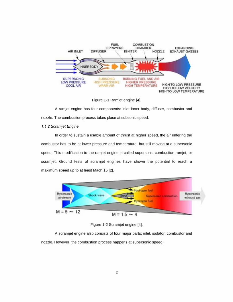
Figure 1-1 Ramjet engine [4].
A ramjet engine has four components: inlet inner body, diffuser, combustor and
nozzle. The combustion process takes place at subsonic speed.
Scramjet Engine
In order to sustain a usable amount of thrust at higher speed, the air entering the
combustor has to be at lower pressure and temperature, but still moving at a supersonic
speed. This modification to the ramjet engine is called supersonic combustion ramjet, or
scramjet. Ground tests of scramjet engines have shown the potential to reach a
maximum speed up to at least Mach 15 [2].
Figure 1-2 Scramjet engine [4].
A scramjet engine also consists of four major parts: inlet, isolator, combustor and
nozzle. However, the combustion process happens at supersonic speed.

3
Nevertheless, scramjet engines still present some drawbacks due to the basic
requirements for an air breathing engine and the limits relating to high airspeed:
- Scramjet needs a working atmosphere dense enough to create large thrust,
which places an upper bound constraint of the flight corridor for scramjet propelled
vehicles.
- Scramjet propelled vehicles are not able to operate at a low altitude due to high
thermal load on the aircraft structure when it flies at a very high speed.
- Scramjets are unable to produce static thrust and only become operationally
efficient at supersonic Mach numbers, thus incapable of taking off on their own and they
need high initial speed for air compression.
These constraints require a complex launch system for a scramjet vehicle. Such
systems typically consists of a carrier aircraft (for take – off) and a rocket to bring the
initial flight Mach number of the scramjet-powered aircraft to about Mach 5. Despite these
disadvantages, scramjet engines are still seen as a bright prospect of hypersonic cruise
and ascent to low-earth-orbit thanks to its light weight and airplane like operation [2].
Dual-mode Scramjet Engine
Curran and Stull introduced the idea of the dual-mode scramjet engine in 1963
[5]. Ramjet and scramjet engines differ from each other in the speed of the flow inside the
combustor, subsonic for ramjet and supersonic for scramjet. The dual-mode scramjet
combines these two flow characteristics in one combustor that can operate in both
regimes depending on the airspeed of the aircraft, hence the name dual-mode scramjet.
Therefore, the dual-mode scramjet has a wider operational Mach number range. This
leads to increased application potential and the possibility of a hypersonic aircraft that
can take off by itself with the help of a turbojet. This turbojet can be used to take the
aircraft to about Mach 3, then the dual-mode scramjet can be used at higher airspeed.

4
Figure 1-3 Dual-mode scramjet engine [3].
Nonetheless, the combination of the two flow regimes in one configuration
introduces some complex phenomena in the isolator and the combustor, which lead to
design and analysis challenges. The flow in the isolator has an intricate structure called
the shock train, formed by the interaction between the inlet exhaust conditions and the
combustor high back pressure, in conjunction with boundary layer separation. This
separation region can spread into the combustor, rendering the flow analysis of this
component more complicated as it switches from ramjet mode to scramjet mode. The
overview of the operation of the isolator and the combustor in a dual-mode scramjet is
described in the next section.
1.2 Operation of Dual-mode Scramjet
Dual-mode Scramjet Combustor
There are two major factors that determine flow properties in the combustor: heat
addition and the change of the combustor area [1].
Regarding heat addition, the Rayleigh flow model shows that:
- At subsonic speed, the flow is accelerated by heat addition.
- At supersonic speed, the flow is decelerated by heat addition.
Regarding area change:
- At subsonic speed, the flow is decelerated as the area increases.
5
- At supersonic speed, the flow is accelerated as the area increases.
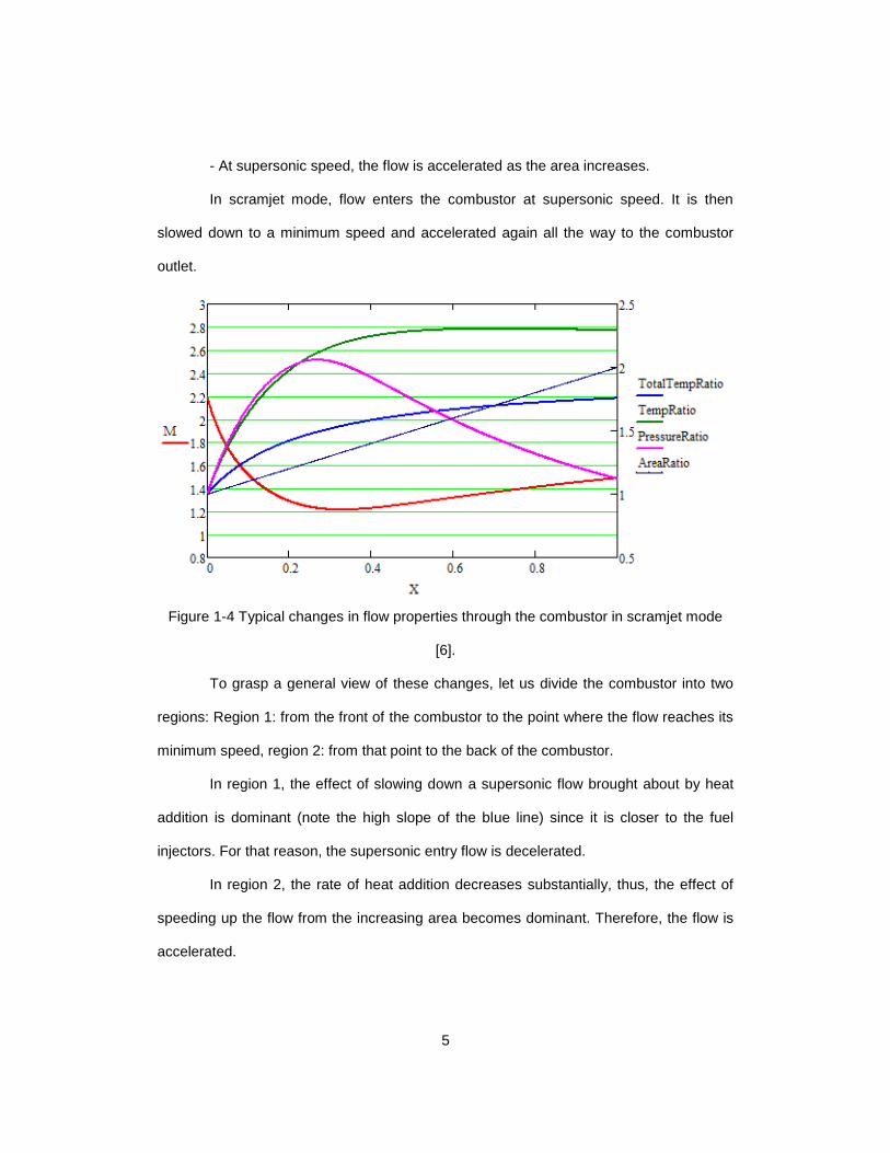
In scramjet mode, flow enters the combustor at supersonic speed. It is then
slowed down to a minimum speed and accelerated again all the way to the combustor
outlet.
Figure 1-4 Typical changes in flow properties through the combustor in scramjet mode
[6].
To grasp a general view of these changes, let us divide the combustor into two
regions: Region 1: from the front of the combustor to the point where the flow reaches its
minimum speed, region 2: from that point to the back of the combustor.
In region 1, the effect of slowing down a supersonic flow brought about by heat
addition is dominant (note the high slope of the blue line) since it is closer to the fuel
injectors. For that reason, the supersonic entry flow is decelerated.
In region 2, the rate of heat addition decreases substantially, thus, the effect of
speeding up the flow from the increasing area becomes dominant. Therefore, the flow is
accelerated.
6
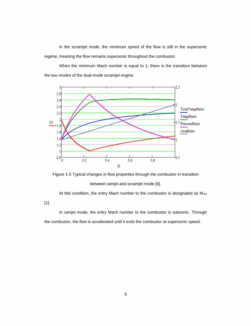
In the scramjet mode, the minimum speed of the flow is still in the supersonic
regime, meaning the flow remains supersonic throughout the combustor.
When the minimum Mach number is equal to 1, there is the transition between
the two modes of the dual-mode scramjet engine.
Figure 1-5 Typical changes in flow properties through the combustor in transition
between ramjet and scramjet mode [6].
At this condition, the entry Mach number to the combustor is designated as M3m
[1].
In ramjet mode, the entry Mach number to the combustor is subsonic. Through
the combustor, the flow is accelerated until it exits the combustor at supersonic speed.

7
Figure 1-6 Typical changes in flow properties through the combustor in ramjet mode [6].
The combustor is divided again into two regions: Region 1: from the front of the
combustor to the point where the flow reaches sonic speed, region 2: the remaining part
of the combustor.
In region 1, the effect of speeding up subsonic flow caused by heat addition is
dominant so the flow is accelerated.
In region 2, the flow enters supersonic regime and thus is slowed down by heat
addition alone. However, as the rate of heat addition decreases substantially, the effect of
the increasing area becomes dominant. Therefore, the flow continues to be accelerated.
At the sonic point, the flow experiences a similar phenomenon to its passage
through a physical throat. However, this is brought about entirely by heat addition as
there is no physical throat in a dual-mode scramjet combustor. The sonic point is, for that
reason, called the thermal throat [1].
8
When calculating flow properties through the combustor, determining the position
of the thermal throat is a critical task as it serves as a starting point to calculate flow
properties at other points in the combustor.
Let us call the entry Mach number to the combustor M3p [1].
Dual-mode Scramjet Isolator
The flow in the isolator will behave according to flow properties at the front
(Station 2) and the back (Station 3) of the isolator.
It has been discovered that the isolator cannot operate with any arbitrary
combination of flow properties at position 2 and 3; there is a limit. With a certain M2, the
isolator cannot generate a M3 below the value equal to the downstream Mach number of
a normal shock wave with the upstream Mach number M2 [1]. In other words, for a
predetermined M3p, the condition under which the isolator and the whole engine can
operate is M2>M2x, with M2x being the Mach number of the flow that will create the Mach
number M3p after a normal shock wave [1].
When the limit mentioned above is satisfied, the isolator can operate in either
one of the three following modes:
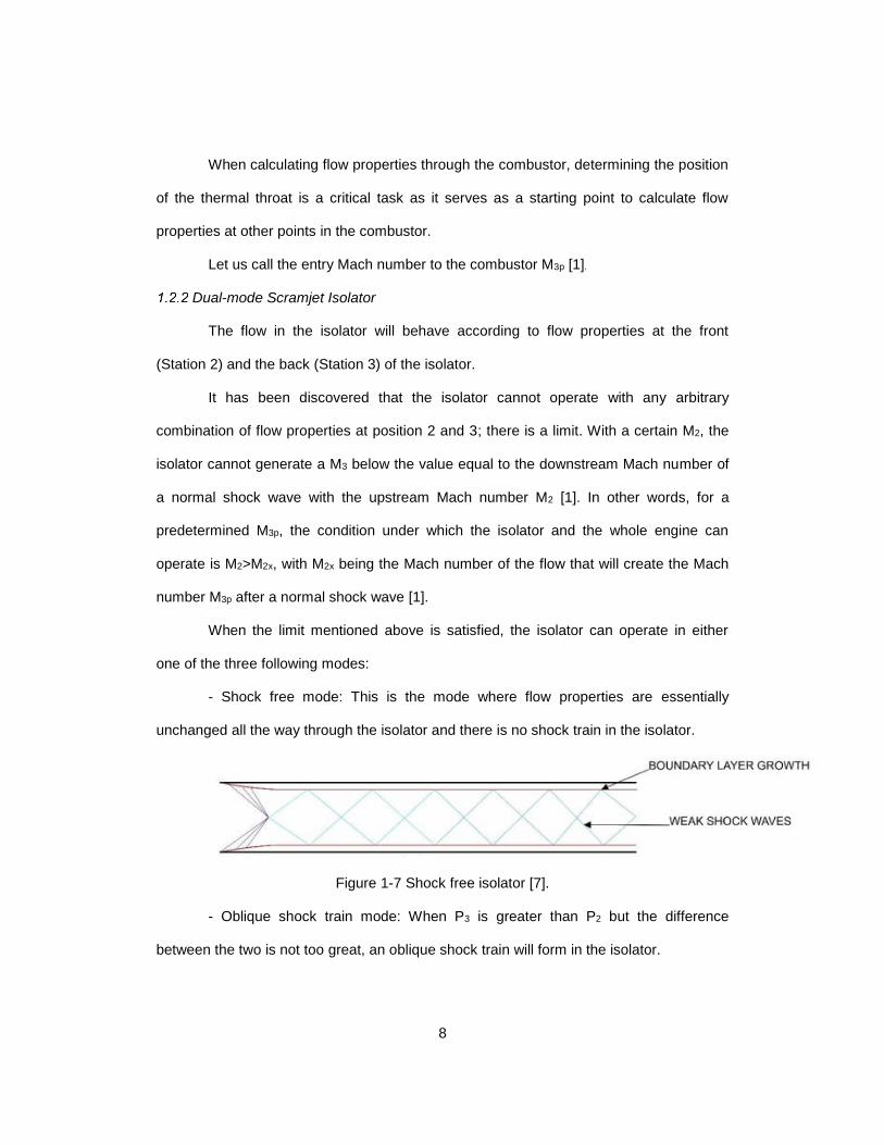
- Shock free mode: This is the mode where flow properties are essentially
unchanged all the way through the isolator and there is no shock train in the isolator.
Figure 1-7 Shock free isolator [7].
- Oblique shock train mode: When P3 is greater than P2 but the difference
between the two is not too great, an oblique shock train will form in the isolator.

9
Figure 1-8 Isolator with oblique shock train [7].
- Normal shock train mode: When the difference between P3 and P2 is large
enough, a normal shock train will form in the isolator.
Figure 1-9 Isolator with normal shock train [7].
The operation of the dual-mode scramjet engine can be summed up as follows:
- When M2< M2x, the engine cannot operate.
- When M2 is between M2x and M3m, the engine will operate in the ramjet mode.
- When M2>M3m, the engine will operate in the scramjet mode.
1.3 Development History
The first scramjet development program was the NASA Hypersonic Research
Engine (HRE) program which started in 1964, with about 52 tests completed [6]. After
this, many other programs in several countries such as Russia, France and Germany
also began. Three prominent projects with successful flight test were the HyShot program
by the University of Queensland in Australia that marked the first flight of a scramjet
propelled aircraft in July 2002 [6], the Hyper-X program [9] and the X-51 program [10].

10
The aircraft designed in the Hyper-X program is called X-43. It has made two successful
flight tests, the first one took place on March 2004 with the aircraft reaching a speed of
Mach 7 and the second one on November 2004. In this second flight, X-43 got to nearly
Mach 10, which set a new speed record [7]. The X-51 program gave birth to the X-51A
Waverider, whose final flight took place on May 1st 2013. In this flight, the aircraft reached
a top speed of Mach 5.1 and travelled on its own scramjet powered engine for four
minutes, making the record for longest scramjet powered flight [12].The most recent
project involving scramjets is the SR-72, the successor of the SR-71 Blackbird. SR-72 is
a hybrid turbojet – scramjet propelled aircraft which is expected to enter service by 2030
[8].
11
Chapter 2
Literature Survey
There have been a number of studies which approach scramjet combustion with
different analysis methods in the past. Presented in this section are some works on this
subject in the literature. The focus is on the methods used for developing a quasi-one-
dimensional flow model of the flow through scramjet combustors and experimental results
that will be used to validate the quasi-one-dimensional code.
2.1 Theoretical Researches
Heiser and Pratt’s Approach
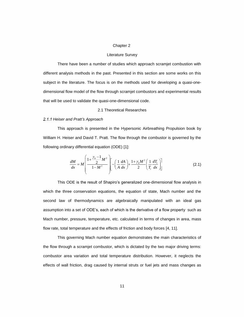
This approach is presented in the Hypersonic Airbreathing Propulsion book by
William H. Heiser and David T. Pratt. The flow through the combustor is governed by the
following ordinary differential equation (ODE) [1]:
22
2
11
11 12
21
b
b t
t
MM dTdM dA
Mdx A dx T dxM
(2.1)
This ODE is the result of Shapiro’s generalized one-dimensional flow analysis in
which the three conservation equations, the equation of state, Mach number and the
second law of thermodynamics are algebraically manipulated with an ideal gas
assumption into a set of ODE’s, each of which is the derivative of a flow property such as
Mach number, pressure, temperature, etc. calculated in terms of changes in area, mass
flow rate, total temperature and the effects of friction and body forces [4, 11].
This governing Mach number equation demonstrates the main characteristics of
the flow through a scramjet combustor, which is dictated by the two major driving terms:
combustor area variation and total temperature distribution. However, it neglects the
effects of wall friction, drag caused by internal struts or fuel jets and mass changes as
12
fuel is being added and mixed into the flow [1]. Moreover, this equation doesn’t take into
account flow separation, which is an important behavior of the flow as the combustion
process generates a high back pressure causing an adverse pressure gradient that
separates the flow. Heiser and Pratt addressed this phenomenon by a constant impulse
function method rather than incorporating it into the ODE [1, 4]. Thus, the variation of the
core flow area in the separation zone is unknown since no position variable is involved in
the control volume analysis.
Ram-Scram Transition and Flame/Shock-Train Interactions in a Model Scramjet
Experiment
The flow model as presented in Heiser and Pratt’s book is applied in this analysis
to study the transition between ramjet and scramjet mode. In ramjet mode, the incoming
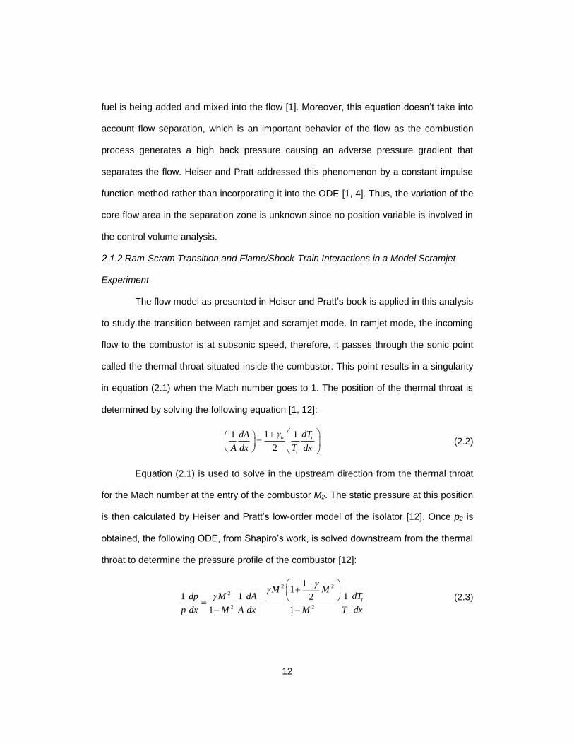
flow to the combustor is at subsonic speed, therefore, it passes through the sonic point
called the thermal throat situated inside the combustor. This point results in a singularity
in equation (2.1) when the Mach number goes to 1. The position of the thermal throat is
determined by solving the following equation [1, 12]:
11 1
2
b t
t
dTdA
A dx T dx
(2.2)
Equation (2.1) is used to solve in the upstream direction from the thermal throat
for the Mach number at the entry of the combustor M2. The static pressure at this position
is then calculated by Heiser and Pratt’s low-order model of the isolator [12]. Once p2 is
obtained, the following ODE, from Shapiro’s work, is solved downstream from the thermal
throat to determine the pressure profile of the combustor [12]:
2 2
2
2 2
11
1 1 12
1 1
t
t
M MdTdp M dA
p dx A dx T dxM M
(2.3)
13
Wall friction and mass addition are neglected and the gas is assumed to consist
of a single species and to be calorically perfect [12]. Moreover, the flow is assumed to
only separate inside the isolator, whereas, it has been found that separation zone also
reaches inside the combustor [16].
Hyshot Program
This is another approach based on the classical quasi-one-dimensional gas
dynamics by Shapiro [16]. This work was done as part of the HyShot program at the
University of Queensland in Australia that has successfully launched a test flight on July
30th, 2002 [16].
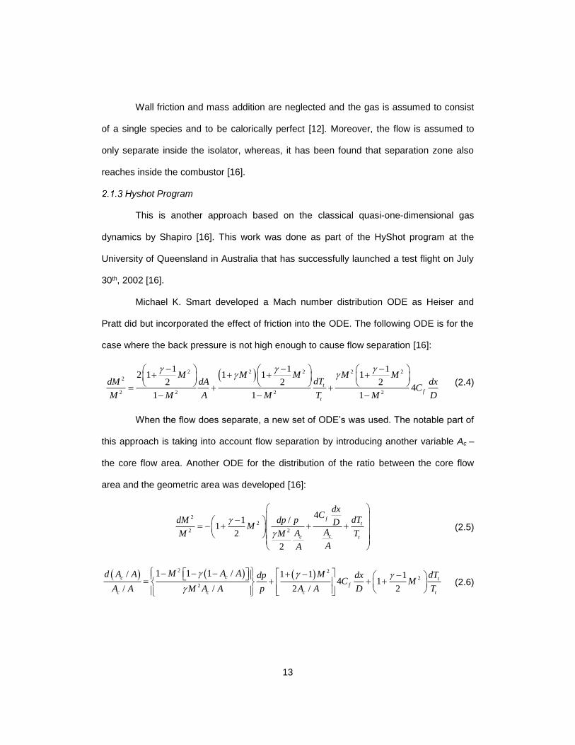
Michael K. Smart developed a Mach number distribution ODE as Heiser and
Pratt did but incorporated the effect of friction into the ODE. The following ODE is for the
case where the back pressure is not high enough to cause flow separation [16]:
2 2 2 2 2
2
2 2 2 2
1 1 12 1 1 1 1
2 2 24
1 1 1
t
f
t
M M M M MdTdM dA dx
CA T DM M M M
(2.4)
When the flow does separate, a new set of ODE’s was used. The notable part of
this approach is taking into account flow separation by introducing another variable Ac –
the core flow area. Another ODE for the distribution of the ratio between the core flow
area and the geometric area was developed [16]:
22
2 2
41 /
12
2
ft
cc t
dxC
dTdM dp p DMAA TM M
AA
(2.5)
2 2
2
2
1 1 1 // 1 1 14 1
/ 2 / 2/
cc t
f
c c tc
M A Ad A A M dTdp dxC M
A A p A A D TM A A
(2.6)
14
This new ODE in conjunction with the Mach number distribution ODE are to be
solved simultaneously by a numerical method. In order to do so, the pressure distribution
term in equation (2.5) and equation (2.6) needs to be an explicit term. It is defined by the
following empirical formula developed by Ortwerth [17, 18]:
2
0
89
2f
H
dp uC
dx D
(2.7)
This model is a lot more comprehensive than the previous one, therefore, offers
more accurate results and better captures the physics of the flow inside a scramjet
combustor. Nonetheless, it still uses the ideal gas assumption whose accuracy
decreases when the temperature in the combustor becomes higher at faster air speed.
2.2 Experimental Researches
Free Piston Shock Tunnel Experiment at University of Queensland – T4 Scramjet:
The free piston shock tunnel uses a free piston to adiabatically compress the
driver gas. A shock wave propagates and reflects from the end wall of the shock tube
after the primary diaphragm rupture. This creates a high enthalpy test gas inside the
reservoir. The enthalpy and pressure of the gas in the reservoir can reach up to 2-15
MJ/kg and 10-80 MPa respectively [16]. The test gas is fed into a nozzle downstream of
the shock tube, where supersonic or hypersonic flow is generated. The duration of such
flow to the test section can reach up to several milliseconds [16].
In order to achieve flows of different Mach number of 4, 6, 8 and 10, several
axisymmetric hypersonic nozzles with different exit to throat area ratios are used. For the
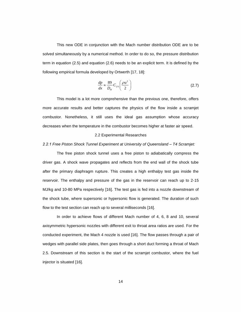
conducted experiment, the Mach 4 nozzle is used [16]. The flow passes through a pair of
wedges with parallel side plates, then goes through a short duct forming a throat of Mach
2.5. Downstream of this section is the start of the scramjet combustor, where the fuel
injector is situated [16].
15
Figure 2-1 T4 scramjet inlet configuration [16].
This configuration generates a supersonic flow of Mach 2.5 with a total pressure
of 1 MPa [16].
Pressure transducers are used to measure the wall pressure. There are 35
pressure transducers 20mm apart of one another [16].
Hyshot 2 Scramjet Flight Experiment
The Center of Hypersonic at the University of Queensland has conducted
scramjet testing in the Mach 7 to Mach 8 range in shock tunnels for many years [17]. A
simplified combustor designed based on the shock tunnel testing is used for two flight
tests which took place at the Woomera Prohibited Area Test Range in central Australia
[17]. The first flight test was on October 30th 2001 but was a failure, a second successful
launch followed on July 30th 2002 [17].
The test flights implement a two-stage Terrier-Orion Mk70 rocket as the
booster, bringing the payload and the second stage Orion motor to a maximum altitude of
more than 300 km [17]. The payload and the second stage motor follow a parabolic

16
trajectory and reenter the atmosphere at 25 to 35 km with the speed of above Mach 7.5
[17]. The reentry provides a useful flight conditions to test the scramjet combustor.
Figure 2-2 Hyshot flight profile [17].
The pressure transducers in use are SenSym 19 C series and SenSym 13 mm
series. There are in total 14 pressure measurements along the wall of the combustor. 13
of which are on the center line starting at 103.6 mm from the combustor entrance and 22
mm apart of each other. Another measurement is made 25 mm offset from the center
line, 290.6 mm from the combustor entrance [17].

17
Figure 2-3 Combustor instrumentation layout [17].
Data are sampled approximately every 2 milliseconds through 48 analog and 4
digital channels [17].
Investigation of the Isolator Flow of Scramjet Engines
This research performs the experiments involving flow through a scramjet
isolator. The experiments are done in the reflected shock tunnel TH2 at the Shock Wave
Laboratory. Helium is used as the working gas [18].
Figure 2-4 Drawing of the hypersonic shock tunnel TH2 [18].

18
The TH2 shock tunnel comprises of three major sections: the high pressure
section, the low pressure section and the nozzle & test section. The high pressure
section and the low pressure section function as a shock tube that drives the test gas.
The test gas is accelerated through the nozzle to the required Mach number in the test
section [18].
Pressure probes prove to provide signal that is much more suitable to determine
the flow structure inside the isolator [18]. Kulite XCQ-080 pressure transducers are used
in the experiment. These pressure transducers have small membrane diameter of 0.7
mm, thus, their natural frequency is relatively high, ranging from 300 to 500 kHz, which
makes them suitable for short measurement time of approximately 1 millisecond [18].
Probes with operating range of 1.7, 7 and 17 bar are needed for the experiment.
17 bar probes are used in the pitot rake, 7 bar probes are used to measure wall pressure
in the shock train region and 1.7 bar probes are used in the upstream region of the
isolator [18].

19
Chapter 3
The Numerical Propulsion System Simulation (NPSS)
This chapter provides a description of the Numerical Propulsion System
Simulation (NPSS) – the platform of the quasi-one-dimensional scramjet combustor code.
3.1 Introduction of NPSS
The simulation of a propulsion system is an intricate process that involves
numerous phenomena from different disciplines. A software devoted to this task needs to
not only have the ability to perform analysis with a low order of fidelity at system level to
achieve basic understanding of the whole system without having to establish a geometry,
but also be capable of zooming to a high enough level of fidelity to accurately simulate
the phenomena happening within each component. In addition, the interaction between
disciplines must be taken into consideration.
While a full system simulation with high order of fidelity will eventually give
detailed results that capture the entire physics of the system, it requires a large amount of
computational resources and takes a long time to reach the final results. For this reason,
it is complicated and unwieldy for establishing a basic understanding of the system in
question [1]. Low order cycle analysis, on the other hand, will provide fast and simple
results that are essential for preliminary analysis of the system. These can also help
anticipate possible problems that will occur during subsequent detailed design process
[19].
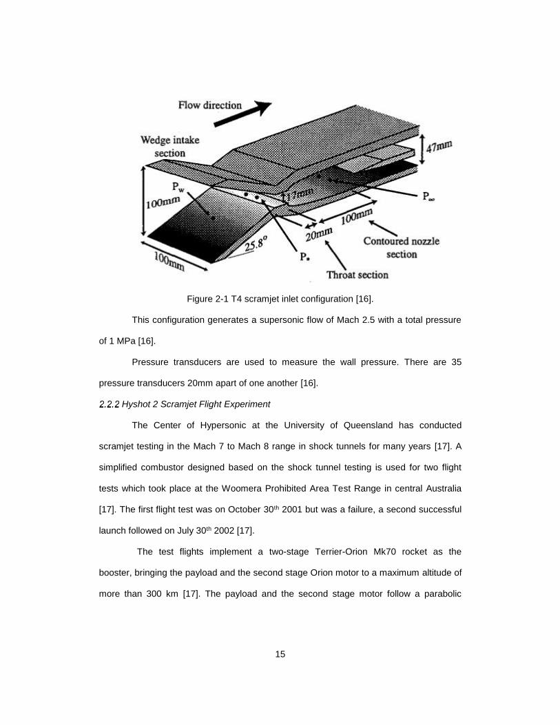
The capability of zooming into different components with different levels of fidelity
is called multifidelity analysis. An example of multifidelity analysis is shown in Figure 3-1,
where the high pressure core of the engine (i.e. compressor, combustor and turbine) is
modeled as a zero-dimensional, aerothermodynamic cycle analysis that is conducted
through the use of component performance maps and the low pressure subsystem (i.e.
20
inlet, fan, core inlet, bypass duct, nozzle) is modeled in 3-dimensions using a CFD
turbomachinery code [20].
Figure 3-1 Hybrid Simulation: 3-Dimensional Low Pressure Subsystem Model Coupled to
a 0-Dimensional High Pressure Core Model [20].
This can be done by isolated analysis, however, the interactions that occur
between components can eventually be masked by the limited communication between
teams or the codes which perform the individual numerical analysis [21]. When working
with today’s highly integrated propulsion systems where multidisciplinary issues can
decrease drastically the overall system performance, this can introduce vital problems
[21]. Thus, it is important that multifidelity analysis be performed by one unique software
that handles all the components in order to ensure communication between components.
The physical processes that take place in an air-breathing gas turbine engine
involves multiple disciplines [20]. For instance, the variations in the geometry of the high-
pressure compressor (casing, blade shape, tip clearances, etc.) that affect the efficiency
and stability of the compressor is determined by aerodynamic, structural, and thermal
loadings. In order to accurately predict the stall margin, simulation of all of these loadings
is required [20]. As a result, to accurately simulate these processes, the coupling of all
involved disciplines needs to be accounted for.

21
The Numerical Propulsion System Simulation (NPSS) is a
multidisciplinary, multifidelity computational simulation tool that meets all the above
requirements. NPSS was developed by NASA in conjunction with other Government
agencies, industries and universities [22]. It serves as a “virtual wind tunnel” that allows
the engine manufacturer to find key design parameters early in the development process
by performing detailed full engine simulations. The use of NPSS could cut the design and
development time and cost by 30 to 40 percent, which is equivalent to $100 million per
year of development, as estimated by a major engine manufacturer [22].
NPSS brings about the following advantages: 1) minimize the expense for
maintaining numerous software systems, 2) ameliorate multidisciplinary team work by
granting all disciplines access to tools and system simulation capability, 3) facilitate
collaboration by providing the industry with a common platform for engine system
simulation, and 4) contain all engine design and operational data in one data base
connected to the system simulation [23].
Alongside gas turbine engines, NPSS usage has also been expanded other
fields such as spacecraft applications and energy applications.
3.2 NPSS Simulation Environment
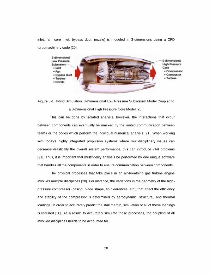
The multidisciplinary framework of NPSS is illustrated in Figure 3-2, where three
primary characteristics of the simulation environment: discipline coupling, component
integration and zooming are shown. This framework allows an engineer to “plug and play”
or “substitute at will” the components of an engine with any combination of 0, 1, 2, 3
dimensional component codes [24].
22
Figure 3-2 Illustration of the NPSS Multidisciplinary Framework [21].
Traditionally, the interaction between different disciplines is handled in a
sequential fashion, with the use of translators to transfer and translate information from
one discipline to the next. This is however lengthy, tedious and often inaccurate [20].
Three coupling techniques are investigated to be included in NPSS: loosely coupled,
process coupled and tightly coupled. Loosely coupled is a rationalized version of the
traditional approach. A component’s aero, thermal and structural response is determined
by separated programs. Then these data are coupled together by a set of generic
translators and a subroutine library [20]. In process coupling, component codes are run
under the control of an automated higher level system, the exchanged information
between the codes is also managed by this system [20]. Tightly coupling connects the
23
disciplines at a fundamental equation level. The matrix representing the whole system is
solved simultaneously by implicit methods [20].
3.3 NPSS Components
Architecture, code language and basic objects
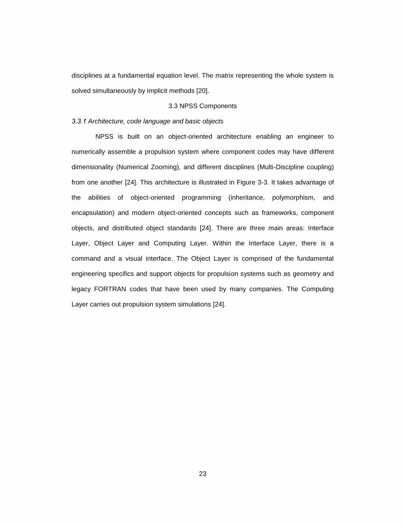
NPSS is built on an object-oriented architecture enabling an engineer to
numerically assemble a propulsion system where component codes may have different
dimensionality (Numerical Zooming), and different disciplines (Multi-Discipline coupling)
from one another [24]. This architecture is illustrated in Figure 3-3. It takes advantage of
the abilities of object-oriented programming (inheritance, polymorphism, and
encapsulation) and modern object-oriented concepts such as frameworks, component
objects, and distributed object standards [24]. There are three main areas: Interface
Layer, Object Layer and Computing Layer. Within the Interface Layer, there is a
command and a visual interface. The Object Layer is comprised of the fundamental
engineering specifics and support objects for propulsion systems such as geometry and
legacy FORTRAN codes that have been used by many companies. The Computing
Layer carries out propulsion system simulations [24].

24
Figure 3-3 NPSS Object-Oriented Open Architecture [22].
NPSS utilizes a C++ type object-oriented programming language [25], with the
following attributes: 1) maximum code reusability, 2) clear data connectivity, and 3) code
modularity [20]. The problem can be divided into objects that consist of useful data and
methods (functions) [26]. The basic objects used for a 0 and 1-dimensional analysis are:
1) elements, 2) subelements, 3) flow stations, 4) ports and 5) tables [24]. This object
structure allows NPSS to have a wide range of applications amongst air breathing,
rocket, fuel cell and ground based power propulsion and more by creating new functional
objects for each particular application [24].
Elements are the building blocks of a model in NPSS. They account for the major
components of the system [27]. Each element is a C++ code can exchange data with
each other [28]. An element can have subelements: element-like objects built to provide
supporting data to the object they accompany [27]. NPSS has various built-in elements
like Ambient, Compressor, Burner, Turbine, Nozzle, Shaft, etc… [29] and subelements
such as CompressorRlineMap, TurbinePRmap, BurnEfficiency, ThermalMass, etc... [29].
25
Users can also define their own elements and subelements that are suitable for their
model. Flow stations are found between elements. Elements communicate with one
another through input and output ports that control the data flow through links. Elements
may have none or an appropriate number of ports needed for their usage [27]. Functions
and tables can also be written to execute special calculations [27].
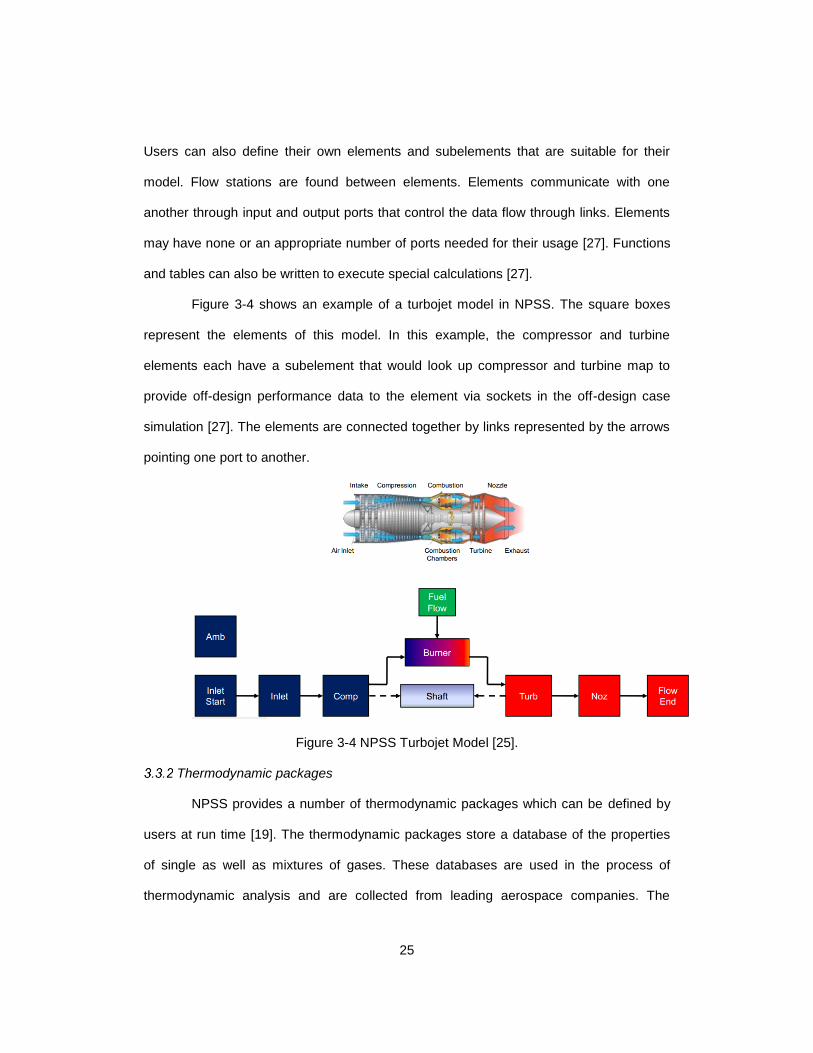
Figure 3-4 shows an example of a turbojet model in NPSS. The square boxes
represent the elements of this model. In this example, the compressor and turbine
elements each have a subelement that would look up compressor and turbine map to
provide off-design performance data to the element via sockets in the off-design case
simulation [27]. The elements are connected together by links represented by the arrows
pointing one port to another.
Figure 3-4 NPSS Turbojet Model [25].
Thermodynamic packages
NPSS provides a number of thermodynamic packages which can be defined by
users at run time [19]. The thermodynamic packages store a database of the properties
of single as well as mixtures of gases. These databases are used in the process of
thermodynamic analysis and are collected from leading aerospace companies. The
26
thermodynamic package is able to perform thermodynamic calculation at molecular level
of the flow under extreme conditions such as gas vibration and dissociation [19]. There
are six thermodynamic packages available in NPSS: 1. GasTbl – Pratt & Whitney air &
fuel properties, 2. allFuel/GEFluid – General Electric air & fuel properties, 3. Janaf –
Honeywell implementation of JANAF package, 4. CEA – NASA’s Chemical Equilibrium
Analysis package, 5. FPT – User customizable package, 6. REFPROP – Interface to
NIST package [30].
Solver
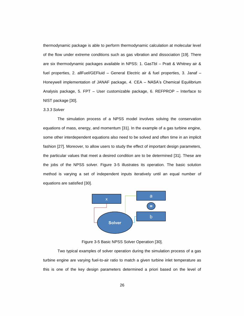
The simulation process of a NPSS model involves solving the conservation
equations of mass, energy, and momentum [31]. In the example of a gas turbine engine,
some other interdependent equations also need to be solved and often time in an implicit
fashion [27]. Moreover, to allow users to study the effect of important design parameters,
the particular values that meet a desired condition are to be determined [31]. These are
the jobs of the NPSS solver. Figure 3-5 illustrates its operation. The basic solution
method is varying a set of independent inputs iteratively until an equal number of
equations are satisfied [30].
Figure 3-5 Basic NPSS Solver Operation [30].
Two typical examples of solver operation during the simulation process of a gas
turbine engine are varying fuel-to-air ratio to match a given turbine inlet temperature as
this is one of the key design parameters determined a priori based on the level of

27
technology of the turbine (the material of the turbine blades); varying incoming air flow
rate to obtain a desired value of engine net thrust. This operation is also called engine
sizing: for a specific thrust requirement, the engine needs a high enough air flow rate to
produce such amount of thrust and this in turn determines the diameter of the engine.

28
Chapter 4
Quasi-one-dimensional Scramjet Isolator and Combustor Model
A quasi-one-dimensional analytical model that is simple enough to reduce the
computational resources and time but is still able to capture the complex physics of the
flow in a scramjet isolator and combustor is described in this chapter.
4.1 Assumptions
The following assumptions are made:
- The flow is quasi-one-dimensional, all parameters are either non dimensional or
the axial position is the only independent spatial variable.
- Steady flow is assumed.
- The working gas is in thermodynamic and chemical equilibrium.
- Body forces are neglected.
4.2 Conservation Equations
The conservations equations are formed based on an elemental control volume
inside the combustor as shown in Figure 4-1:
Figure 4-1 Schematic of elemental control volume for burner analysis [7].

29
Conservation of Mass
The conservation equation of mass is given by:
cm uA (4.1)
Where the core flow area can be determined as the geometric area minus the
separation area and the area of the fuel jet [7]:
c sep jetA A A A (4.2)
Conservation of Momentum
The conservation equation of momentum is expressed in form of the change of
static pressure across the elemental control volume [1, 11, 7]:
21
2
fx w
f
c
u u Adp du dmu u C
dx dx A dx Adx
(4.3)
Let m
I be:
21
2
fx w
m f
c
u u AdmI u C
A dx Adx
(4.4)
Therefore:
m
dp duu I
dx dx (4.5)
Conservation of Energy
The change in the enthalpy of the flow is due to the heat added by the burnt fuel
and the heat flux through the combustor wall. This is the conservation of energy [1, 7]:
2 1
2
nf w
tf
q Adh du u dmu h h
dx dx m dx mdx
(4.6)
Let e
I be:

30
2 1
2e
nf w
tf
q Au dmh h
m dx mdxI
(4.7)
We have:
e
dh duu I
dx dx (4.8)
Written in terms of total enthalpy, equation (4.8) becomes:
t
e
dhI
dx (4.9)
We now have the three conservation equations which serve as the basis for the
quasi-one-dimensional analytical model. The modification that needs to be made
accordingly to each component will be described in the following sections.
4.3 Combustor Analytical Model
Algebraic Manipulation Involving the Conservation Equations
First, take the derivative of the conservation equation of mass, from equation
(4.1), we obtain:
c
c
dAdu u u d u dm
dx A dx dx m dx
(4.10)
Substitute the derivative of flow velocity into equation (4.5) and (4.8):
2 22c
m
c
dAdp u d u dmu I
dx A dx dx m dx
(4.11)
and:
2 2 2
c
e
c
dAdh u u d u dmI
dx A dx dx m dx
(4.12)
As a common procedure in CEA, the derivative of each flow property can be
calculated from those of static pressure and static temperature. In this case, the usage of
static enthalpy as one of the independent variables instead of static temperature proves

31
to be more convenient as we already establish an equation involving the rate of change
of static enthalpy. In addition, another independent variable is introduced because there
is fuel added and burnt in the flow. The third independent variable is the equivalence ratio
.
The derivative of density can be written as follows:
d dp dh d
dx p dx h dx dx
(4.13)
Each of the three partial derivatives is calculated using the finite difference
method.
Substitute equation (4.13) into equations (4.11) and (4.12), we will have a system
of two equations in which dp
dx and
dh
dx are treated as unknowns. Solving for these two
quantities and combining them with equation (4.9), we arrive at three equations of the
following forms:
, , t
dpf p h h
dx (4.14)
and:
, , t
dhf p h h
dx (4.15)
and:
, ,t
t
dhf p h h
dx (4.16)
These are the ultimate forms that can be solved numerically by the 4th order
Runge-Kutta marching scheme, which will be outlined in the next section.

32
Friction Coefficient
The reference temperature method is used to determine the friction coefficient
and later the wall heat flux.
First, we need to determine if the flow is laminar or turbulent. This is done by
comparing the Reynolds number of the flow to the transition Reynolds number ReT which
is computed as follows [7]:
-4 2.641log Re 6.421exp 1.209 10T M (4.17)
If the flow Reynolds number is higher than the transition Reynolds number, it is
turbulent, otherwise, it is laminar.
The second step is to compute the reference temperature.
- For laminar flow [7]:
0.5 2
*0.16Pr 1
0.45 0.552
W
TMT T T
(4.18)
- For turbulent flow [7]:
1/3 2
*0.16Pr 1
0.5 0.52
W
TMT T T
(4.19)
where: WT is the wall temperature and Pr is the Prandtl number.
Thirdly, the reference Reynolds number is calculated as follows [7]:
**
*Re
uD
(4.20)
The reference density and viscosity are assumed to vary with temperature and
are computed as follows [1, 7]:
*
*
T
T
(4.21)
and:
33
3/2*
*
*
111
111
T T K
T T K
(4.22)
Lastly, the friction coefficient is determined from the reference Reynolds number:
- For laminar flow [7]:
*
0.664
RefC (4.23)
- For turbulent flow [7]:
0.139
*
0.02296
RefC (4.24)
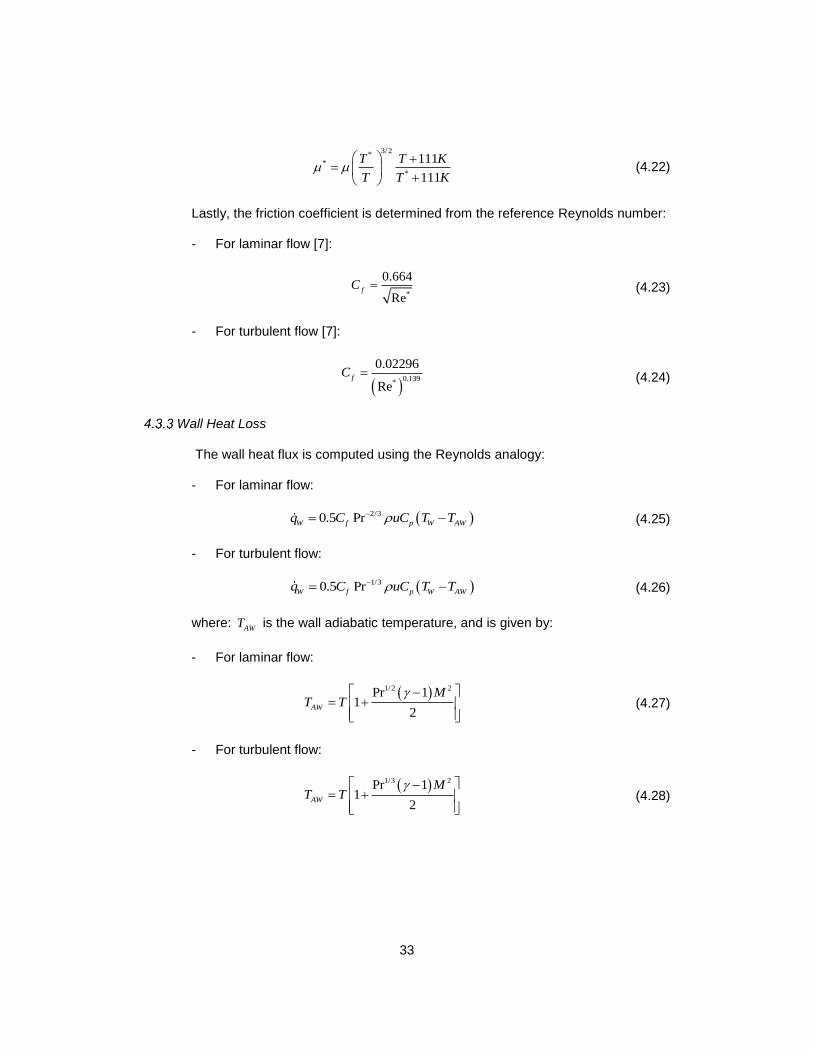
Wall Heat Loss
The wall heat flux is computed using the Reynolds analogy:
- For laminar flow:
2/30.5 PrW f p W AWq C uC T T (4.25)
- For turbulent flow:
1/30.5 PrW f p W AWq C uC T T (4.26)
where: AWT is the wall adiabatic temperature, and is given by:
- For laminar flow:
1/2 2Pr 11
2AW
MT T
(4.27)
- For turbulent flow:
1/3 2Pr 11
2AW
MT T
(4.28)

34
Mixing Efficiency Curve
Not all the fuel injected into the air stream is mixed and burned. The area of the
unmixed stream together with the separation area will compress the core flow area as
equation (4.2) indicates. Thus, a mixing model is necessary to determine the amount of
fuel that is mixed and burned as well as that of the unmixed fuel and its area.
There are different formula developed from experiments that are specific to
certain type of fuel and injection scheme.
The simplest one is a curve fit proposed by Heiser and Pratt as follows [1]:
3
4 3
,
3
4 3
( )
1 1
m c tot
x x
x xx
x x
x x
(4.29)
where: ,c tot is the mixing efficiency at the end of the combustor, ϑ is an
empirical constant whose value is from 1 to 10 [5]. This constant will determine which
injection scheme the curve is fitted to. It has been observed that lower values of ϑ
correspond to parallel injection and higher values results in a curve resembling to that of
normal injection scheme.
The following are a couple of the aforementioned empirical formula that will be
used for the code validation:
- Strut mixing model for hydrogen fuel:
The mixing efficiency is given by [7]:
( ) 1 mix
kx
L d
m x e
(4.30)
mixL is the mixing length and can be determined as follows:
35
*
( )
f f f
mix
c a a
D K uL
f M u
(4.31)
where: 23
( ) 0.25 0.75 cM
cf M e
and f a
c
f a
u uM
a a
, k, d and *K are constant and take the following values: a = 1.065, k = 3.696,
d = 0.806 and * 390K
fD is the fuel jet diameter.
cM is the convective Mach number and is calculated from fuel velocity and air
velocity as well as their acoustic speed.
- Normal injection model for hydrogen fuel:
The mixing efficiency is given by [7, 35]:
( ) 1.01 0.176lnm
xx
x
(4.32)
where:
1.720.179 mixx L e
(4.33)
The mixing length in this case is estimated to be 60 times the spacing between
injectors.
From the mixing efficiency, the area of the unmixed fuel jet is given by [7]:
,3( ) 1 ( )jet jet cA x A x (4.34)
where: Ajet,3 is the fuel jet area at Station 3.
NPSS Calculation Procedure
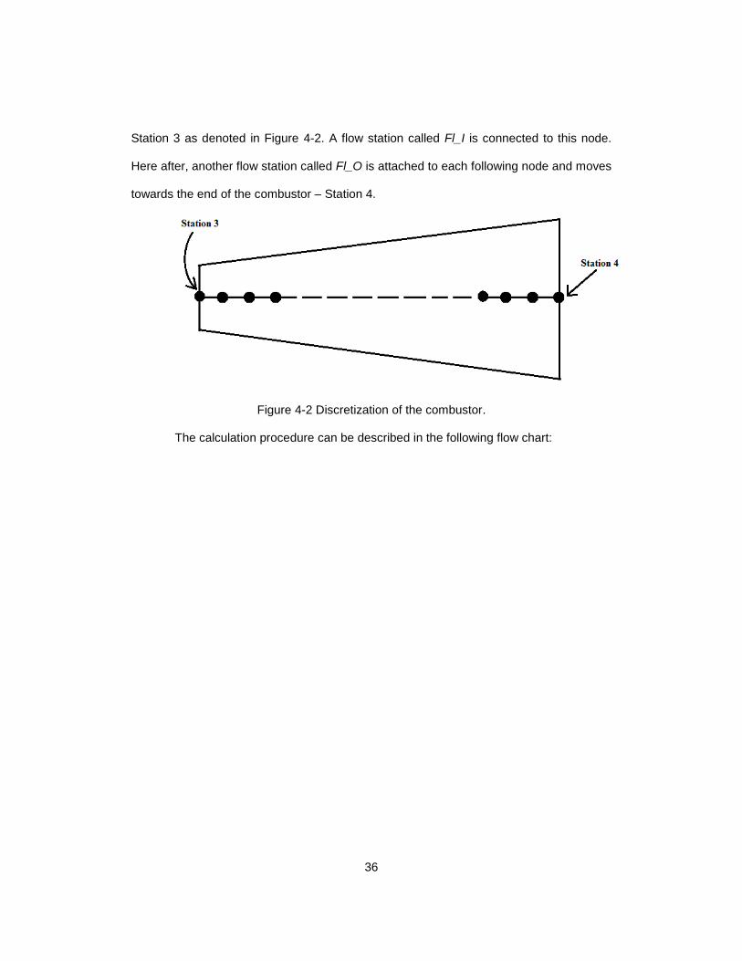
The combustor is “discretized” into n infinitesimal elements of length dx which is
the same as the aforementioned elemental control volume. This corresponds to n+1
nodes along the axis of the combustor. The first node is at the entry of the combustor –
36
Station 3 as denoted in Figure 4-2. A flow station called Fl_I is connected to this node.
Here after, another flow station called Fl_O is attached to each following node and moves
towards the end of the combustor – Station 4.
Figure 4-2 Discretization of the combustor.
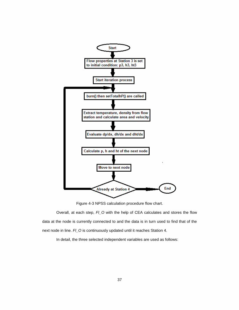
The calculation procedure can be described in the following flow chart:
37
Figure 4-3 NPSS calculation procedure flow chart.
Overall, at each step, Fl_O with the help of CEA calculates and stores the flow
data at the node is currently connected to and the data is in turn used to find that of the
next node in line. Fl_O is continuously updated until it reaches Station 4.
In detail, the three selected independent variables are used as follows:
38
- Static enthalpy and static pressure of the flow are inserted into CEA through
the use of a flow station function called setTotalhP(), which in turn gives out
static temperature and density.
- Flow velocity is calculated from total enthalpy and static enthalpy:
2 tu h h (4.35)
Core flow area is determined from the geometric area and the fuel jet area.
In order to calculate the enthalpy change due to the burnt fuel, a built-in function
in NPSS call burn() is used. This function will add and burn the fuel with the air. It keeps
pt of the mixture the same and calculate ht based on the amount of fuel added and the
hpr of the fuel. In this code, p, h and ht is given and the mixture properties are to be set
by those parameters. Thus, the burn() function is first used beforehand to add and burn
the fuel first, then setTotalhP() is used to set flow properties to the right values.
With these properties and with the three numerically calculated values of partial
derivative of density:p
,
h
and
, we now have all the needed variables to plug into
equations (4.14), (4.15) and (4.16) to calculate the derivative of static pressure, static
enthalpy and total enthalpy. Based on these derivatives, the values of p, h and ht at the
next node are determined as follows:
1i i
dpp p x
dx (4.36)
and:
1i i
dhh h x
dx (4.37)
and:
39
1i i
t
t t
dhh h x
dx (4.38)
where the terms: dp/dx, dh/dx and dht/dx are weighted average slope value
calculated from the 4 approximate values as outlined in the 4th order Runge-Kutta
procedure.
The process is repeated until the end of the combustor.
4.4 Isolator Analytical Model
Empirical Formula of Pressure Distribution
The isolator is simpler than the combustor in the sense that it is usually a
constant area duct and there is no heat addition from fuel. However, the flow is bound to
separate, which introduces another unknown to the analytical model: the core flow area.
Thus, another equation is required to make the set of equations solvable and further
modification to the original conservation equations is also needed.
The added equation is the specified pressure distribution. This is an empirical
formula developed by Ortwerth [18, 17] based on experimental data with different Mach
number, Reynolds number and duct geometry:
0
289
2f
H
dp uC
dx D
(4.39)
where: HD is the hydraulic diameter of the duct and
0fC is the friction coefficient
at the separation start point [17].
As we now have an explicit pressure distribution from equation (4.39), we can
eliminate the du/dx term in both equations (4.5) and (4.8), resulting in a new equation
calculating the derivative of static enthalpy:
1 m
e
Idh dpI
dx dx (4.40)
40
Equations (4.39), (4.40) and (4.9) are used for the 4th order Runge-Kutta method
in the case where flow separation occurs.
NPSS Calculation Procedure
The isolator is divided into two regions: the attached region and the separated
region.
In the attached region where flow remains attached, the same equations and
calculation procedure as the one implemented for the combustor the combustor is used.
Heat addition from fuel is not present so there is no need to use the burn() function.
In the separation region, generally the same NPSS calculation procedure is
used, the only difference is that core flow area is now a new unknown and is calculated
from flow rate, velocity and density using the conservation equation of mass. Therefore,
we will also have core flow area distribution as an output of the quasi-one-dimensional
code.
The point separating these two regions is the separation start point xu. This point
will be iterated until the Mach number or pressure at Station 3 matches the specified
value given in the experimental data.

41
Chapter 5
Results
This chapter describes the quasi-one-dimensional code validation by comparison
to experimental data available in the literature.
5.1 Combustor Code Validation
The first validation is done by comparing the results of the analytical model to
that of the experimental results obtained from the T4 free piston shock tunnel experiment
conducted at the University of Queensland [16].
The geometry of the combustor section in the T4 experiment is shown in the
following figure:
Figure 5-1 T4 scramjet geometry [7].
The combustor is a diverging duct with a rectangular initial cross section of
dimension 0.047 m x 0.1 m. The upper and lower walls diverge symmetrically at an angle
of 1.720 over a length 0.8 m [7, 33].
42
The fuel injector is a strut type injector with a 0.0016 m slot width. Hydrogen fuel
is injected parallel to the incoming airflow at the point where the combustor cross section
starts to increase. Fuel is injected at sonic speed [7].
There are three cases in the experiment. All have the same incoming condition
and same wall temperature of 300 K but the equivalence ratio is varied. The inlet
conditions along with the equivalence ratio of each case are shown in the following table
[33, 7]:
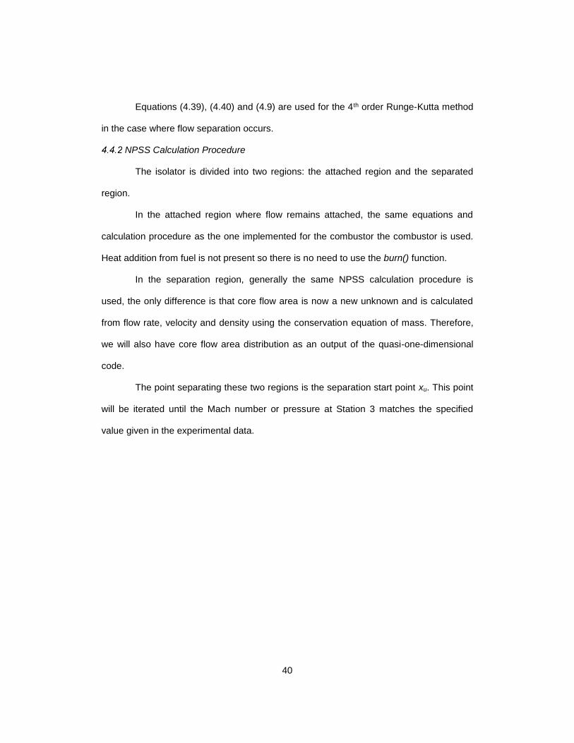
Table 5-1 T4 experiment data
Case M3 P3 (kPa) T3 (K) Equivalence ratio
1 2.47 59 1025 0.19
2 2.47 59 1025 0.38
3 2.47 59 1025 0.58
In order to model the mixing efficiency of this experiment, the hydrogen fuel strut
injector empirical formula described in Section 4.3.4 is used.
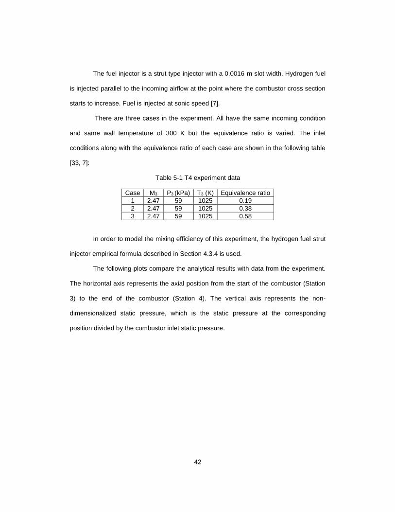
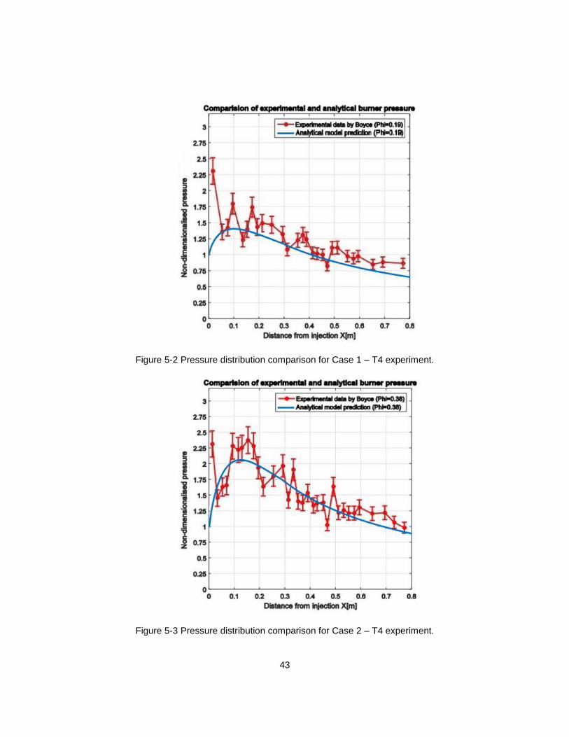
The following plots compare the analytical results with data from the experiment.
The horizontal axis represents the axial position from the start of the combustor (Station
3) to the end of the combustor (Station 4). The vertical axis represents the non-
dimensionalized static pressure, which is the static pressure at the corresponding
position divided by the combustor inlet static pressure.
43
Figure 5-2 Pressure distribution comparison for Case 1 – T4 experiment.
Figure 5-3 Pressure distribution comparison for Case 2 – T4 experiment.

44
Figure 5-4 Pressure distribution comparison for Case 3 – T4 experiment.
Figures 5-2 to 5-4 shows that the quasi-one-dimensional code provides
reasonably accurate results that agree with the experimental data. The pressure
increases sharply initially due to the effect of heat addition from burnt fuel then decreases
after reaching a peak value. Fuel is mixed and burnt more efficiently right after the
injector. After the point of maximum pressure, other effects, i.e. friction, heat loss and
area expansion become more dominant. The initial pressure spike can be the result of
the shockwave created by the injector strut. It can also be seen that with higher
equivalence ratio, meaning more fuel is burnt, higher peak pressure is observed. This
peak pressure is the cause of shock train inside the isolator.
The second validation is carried out by comparison to the experimental results
obtained from the Hyshot 2 flight test data [17].
The geometry of the Hyshot 2 scramjet is described in the following figures:

45
Figure 5-5 Schematic of Hyshot 2 scramjet geometry (dimensions are in millimeters) [17].
Figure 5-6 Hyshot 2 combustor section geometry [7].
The combustor is a constant area duct with a rectangular initial cross section of
dimension 0.0098 m x 0.075 m. The internal nozzle section after the combustor expands
at an angle of 120. The length of the constant area section is 0.242 m from the fuel
injection position and the internal nozzle spreads over a length of 0.147 m [7].
The fuel injector is a normal injection type where hydrogen fuel enters the
incoming flow at a 90 degree angle. The position of the fuel injector is 0.058 m
downstream of the combustor entrance plane. Fuel is injected at sonic speed [7, 17].
The flight test data comprises of two categories: unfueled combustor and fueled
combustor, each of which contains 4 cases [17]. One case from each category is chosen
for comparison with the quasi-one-dimensional code output. The wall temperature is
46
assumed to be constant at 350 K [7]. The other combustor entrance data are shown in
the following table:
Table 5-2 Hyshot 2 experiment data
Case M3 P3 (kPa) T3 (K) Equivalence ratio
1 (unfueled) 2.436 55.256 1388.4 0
2 (fueled) 2.393 44.847 1416.6 0.346
The hydrogen normal injection empirical formula described in Section 4.3.4 is
used to model the mixing efficiency.
For each case, the non-dimensionalized static pressure, which is the static
pressure at the corresponding position divided by the combustor inlet static pressure is
plotted versus the axial position from the injection point to the end of the combustor. The
comparison to the flight data is as follows:
Figure 5-7 Pressure distribution comparison for Case 1 – Hyshot 2.
47
Figure 5-8 Pressure distribution comparison for Case 2 – Hyshot 2.
Once again, the results show agreement between the analytical data and the
flight test data. This also validates the accuracy of the normal injection mixing efficiency
curve in modeling the heat addition process.
To conclude the combustor validation, it can be stated that the quasi-one-
dimensional code has been validated with experimental data and provided accurate
results in terms of the pressure distribution through the combustor.
5.2 Isolator Code Validation
The isolator code is essentially the same analytical model as the combustor code
with modification to the system of differential equations by adding a prescribed pressure
distribution and removing heat addition. The validation of this modified code is done by
comparing its results to that of the experiments done in the reflected shock tunnel TH2 at
the Shock Wave Laboratory by Fisher [18].

48
The following figure describes the schematic of the isolator in the experiment:
Figure 5-9 Heated isolator experiment setup [7].
The isolator is a duct with rectangular cross section. The length of the isolator is
0.2067 m but the pressure probe for the back pressure is at 0.18 m from Station 2 [18],
thus, the length used for the code is 0.18 m. The height and width of the isolator are
0.018 m and 0.1 m respectively [18]. The gas used in the experiment is Helium [18].
Two cases are chosen for validation. All have the same wall temperature of 1000
K except for the first case which is run at wall temperature of 300 K and the same inlet
condition which is shown in the following table:
Table 5-3 Fisher experiment data
Case M2 P2 (kPa) T2 (K) M3
1 3.5 12.440 333 3.4
2 3.5 12.440 333 2.4
3 3.5 12.440 333 2.3
4 3.5 12.440 333 2.1
The Mach number at the end of the isolator M3 in each case is prescribed. The
validation procedure is done by iterating the location of the separation start point until the
back pressure obtained from the code matches the experimental data except for the first
49
case, where no separation occurs. Static wall pressure is then compared between the
analytical results and experimental results to assess the accuracy of the code.
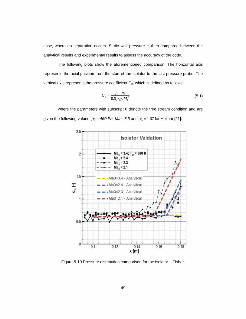
The following plots show the aforementioned comparison. The horizontal axis
represents the axial position from the start of the isolator to the last pressure probe. The
vertical axis represents the pressure coefficient Cp, which is defined as follows:
0
2
0 0 00.5p
p pC
p M
(5.1)
where the parameters with subscript 0 denote the free stream condition and are
given the following values: p0 = 460 Pa, M0 = 7.5 and 0 1.67 for Helium [21].
Figure 5-10 Pressure distribution comparison for the isolator – Fisher.

50
The Mach number at Station 3 obtained from the code is compared to the
prescribed values as follows:
Table 5-4 Ma3 comparison – Fisher experiment
Case Ma3 - Analytical Ma3 - Experimental Error (%)
1 3.203 3.4 6.150%
2 2.677 2.4 10.347%
3 2.595 2.3 11.368%
4 2.395 2.1 12.317%
The error increases as the shock train lengthens. This indicates that the
reference temperature method over predicts the pressure coefficient, which in turn makes
the slope of the pressure line become stiffer than the experimental data. This becomes
more prominent as the shock train length increases.
It can be seen that the analytical results demonstrate reasonable accuracy in
terms of separation start point and pressure gradient across the shock train. However,
the given data only represent wall pressure. The flow structure inside an isolator is rather
complex due to shock train formation, thus, the pressure of the flow changes from the
center line outwards and is different from the wall pressure. As a result, a higher order
analysis is needed to obtain a complete pressure distribution of the isolator.
The modification of the combustor code only provides limited information on
predicting the separation start point, which in turn can be used to determine the length of
the isolator in the preliminary step of the design process.
51
Chapter 6
Conclusion
A summary of the work done in this thesis as well as some aspects of future work
are presented in this chapter.
6.1 Summary
A quasi-one-dimensional analytical model has been developed to solve for flow
properties inside a scramjet combustor. The basis of the model is the conversation
equations of mass, momentum and energy combined with thermodynamics and concepts
of boundary layer theory. The analytical model treats the working fluid as real reacting
gas in equilibrium and takes into account the following aspect of the physics of flow
through a scramjet combustor: geometric area change, friction, wall heat loss and the
heat addition from the reaction of the air and fuel. A 4th order Runge-Kutta method is
chosen to be the numerical integration scheme as it is one of the methods that provide
results of high order of accuracy and the algebraic manipulation of the differential
equations to arrive at the form outlined in this scheme is straight forward.
The platform for code development is the Numerical Propulsion System
Simulation (NPSS), which allows multidiscipline and multifidelity analysis as well as
provides the flexibility of model customization. Thus, the NPSS code can be easily
reused and expanded beyond the application to scramjet engines.
A modification to the system of governing equation is also made to solve for the
flow through the isolator by prescribing a pressure gradient. Although this model only
provides limited information of separation start point and wall pressure, the data obtained
is crucial in determining the length of the isolator, which is an important parameter in the
preliminary design process.
52
The code is validated by comparing its results to multiple experimental and flight
test data. The comparison shows that the code provides results with acceptable level of
accuracy, both for the combustor and isolator.
6.2 Future Work
Some aspects of the current work can be expanded as follows:
• Mixing efficiency of different fuel other than hydrogen
• Interaction between the combustor and isolator
• Validation of said interaction

53
Appendix A
4th order Runge-Kutta Method

54
The 4th order Runge-Kutta method is a numerical method used to solve differential
equations that take the form as follows:
,dx
f x tdt
The essence of this method is calculating 0
x x t t from a known 0 0
x x t by
estimating the slope k of the line connecting the two points.
The slope k is estimated as follows:
1 0 0
,k f x t
2 0 1 0,
2 2
t tk f x k t
3 0 2 0,
2 2
t tk f x k t
4 0 3 0
,k f x k t t t
1 2 3 42 2
6
k k k kk
Having obtained k, we can easily calculate x:
0 0
x x t t x k t
From the point that we have just calculated, we can continue to calculate
0
2x x t t and so on until we reach the end of the concerned domain.
For a system of numerous equations, the same procedure is applied for each unknown.
Each differential equation is calculated based on all the values of unknowns found at each step.

55
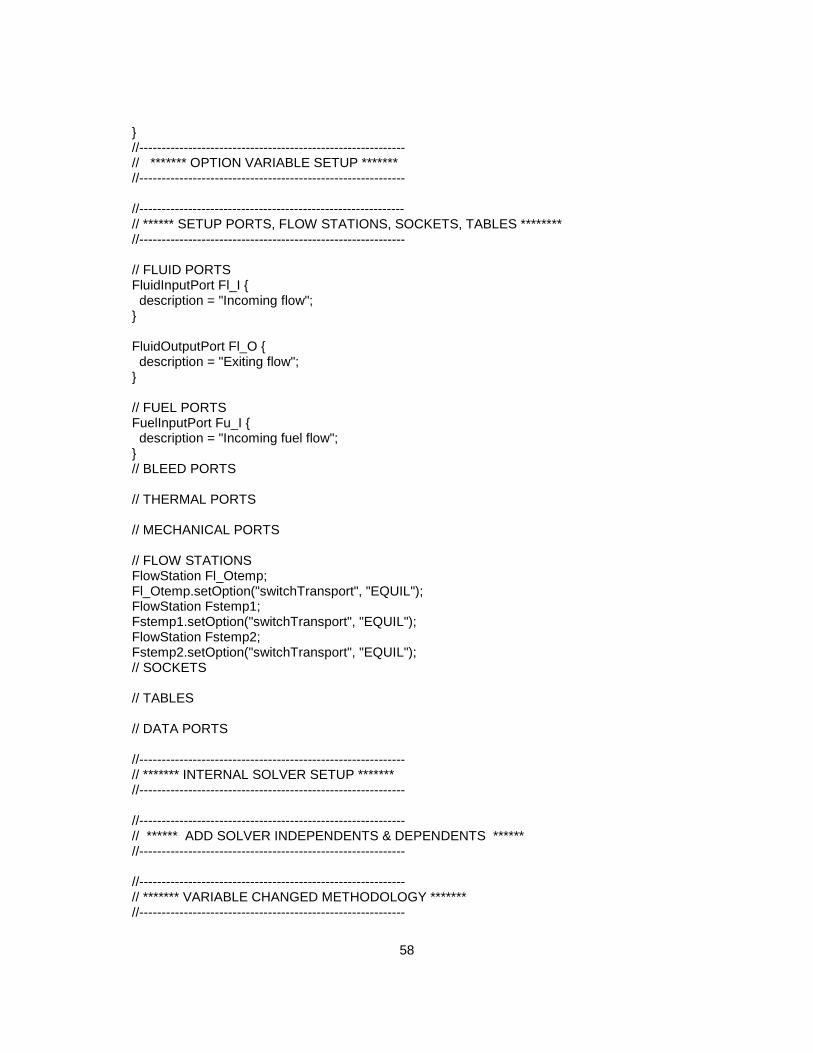
Appendix B
Code outline
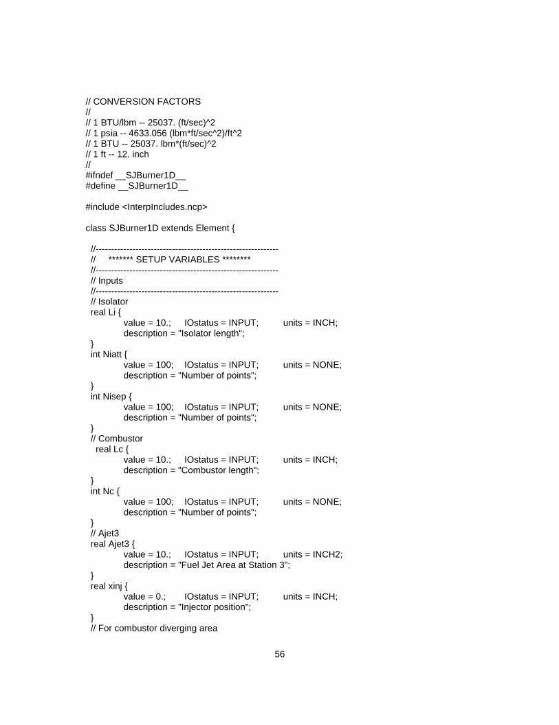
56
// CONVERSION FACTORS // // 1 BTU/lbm -- 25037. (ft/sec)^2 // 1 psia -- 4633.056 (lbm*ft/sec^2)/ft^2 // 1 BTU -- 25037. lbm*(ft/sec)^2 // 1 ft -- 12. inch // #ifndef __SJBurner1D__ #define __SJBurner1D__ #include <InterpIncludes.ncp> class SJBurner1D extends Element { //------------------------------------------------------------ // ******* SETUP VARIABLES ******** //------------------------------------------------------------ // Inputs //------------------------------------------------------------ // Isolator real Li { value = 10.; IOstatus = INPUT; units = INCH; description = "Isolator length"; } int Niatt { value = 100; IOstatus = INPUT; units = NONE; description = "Number of points"; } int Nisep { value = 100; IOstatus = INPUT; units = NONE; description = "Number of points"; } // Combustor real Lc { value = 10.; IOstatus = INPUT; units = INCH; description = "Combustor length"; } int Nc { value = 100; IOstatus = INPUT; units = NONE; description = "Number of points"; } // Ajet3 real Ajet3 { value = 10.; IOstatus = INPUT; units = INCH2; description = "Fuel Jet Area at Station 3"; } real xinj { value = 0.; IOstatus = INPUT; units = INCH; description = "Injector position"; } // For combustor diverging area

57
real a1 { value = 1.; IOstatus = INPUT; units = INCH2; description = "First Coeff"; } real a2 { value = 1.; IOstatus = INPUT; units = INCH2; description = "Second Coeff"; } real xa2 { value = 1.; IOstatus = INPUT; units = INCH; description = "a2 position"; } real a3 { value = 1.; IOstatus = INPUT; units = INCH2; description = "Third Coeff"; } // Wall Temperature real Tw { value = 1080.; IOstatus = INPUT; units = RANKINE; description = "Wall temperature"; } real Pr { value = 0.72; IOstatus = INPUT; units = NONE; description = "Prandtl number"; } // FAR stoic real FARstoic { value = 0.0674; IOstatus = INPUT; units = NONE; description = "Stoichiometric FAR"; } real phi0 { value = 0.0291; IOstatus = INPUT; units = NONE; description = "Initial equivalence ratio"; } //------------------------------------------------------------ // Outputs //------------------------------------------------------------ real Vout { value = 0; IOstatus = OUTPUT; units = FT_PER_SEC; description = "Velocity"; } real Psout { value = 0; IOstatus = OUTPUT; units = PSIA; description = "Static Pressure"; } real Tsout { value = 0; IOstatus = OUTPUT; units = RANKINE; description = "Static Temperature"; } real MNout { value = 0; IOstatus = OUTPUT; units = NONE; description = "Mach Number";
58
} //------------------------------------------------------------ // ******* OPTION VARIABLE SETUP ******* //------------------------------------------------------------ //------------------------------------------------------------ // ****** SETUP PORTS, FLOW STATIONS, SOCKETS, TABLES ******** //------------------------------------------------------------ // FLUID PORTS FluidInputPort Fl_I { description = "Incoming flow"; } FluidOutputPort Fl_O { description = "Exiting flow"; } // FUEL PORTS FuelInputPort Fu_I { description = "Incoming fuel flow"; } // BLEED PORTS // THERMAL PORTS // MECHANICAL PORTS // FLOW STATIONS FlowStation Fl_Otemp; Fl_Otemp.setOption("switchTransport", "EQUIL"); FlowStation Fstemp1; Fstemp1.setOption("switchTransport", "EQUIL"); FlowStation Fstemp2; Fstemp2.setOption("switchTransport", "EQUIL"); // SOCKETS // TABLES // DATA PORTS //------------------------------------------------------------ // ******* INTERNAL SOLVER SETUP ******* //------------------------------------------------------------ //------------------------------------------------------------ // ****** ADD SOLVER INDEPENDENTS & DEPENDENTS ****** //------------------------------------------------------------ //------------------------------------------------------------ // ******* VARIABLE CHANGED METHODOLOGY ******* //------------------------------------------------------------
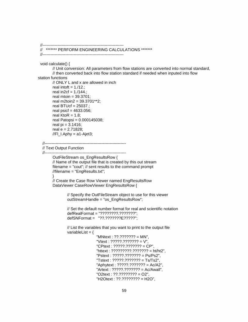
59
//------------------------------------------------------------ // ******* PERFORM ENGINEERING CALCULATIONS ******* //------------------------------------------------------------ void calculate() { // Unit conversion: All parameters from flow stations are converted into normal standard, // then converted back into flow station standard if needed when inputed into flow station functions // ONLY L and x are allowed in inch real intoft = 1./12.; real in2cf = 1./144.; real mtoin = 39.3701; real m2toin2 = 39.3701**2; real BTUcf = 25037.; real psicf = 4633.056; real KtoR = 1.8; real Patopsi = 0.000145038; real pi = 3.1416; real e = 2.71828; //Fl_I.Aphy = a1-Ajet3; //------------------------------------------------------------ // Text Output Function //------------------------------------------------------------ OutFileStream os_EngResultsRow { // Name of the output file that is created by this out stream filename = "cout"; // sent results to the command prompt //filename = "EngResults.txt"; } // Create the Case Row Viewer named EngResultsRow DataViewer CaseRowViewer EngResultsRow { // Specify the OutFileStream object to use for this viewer outStreamHandle = "os_EngResultsRow"; // Set the default number format for real and scientific notation defRealFormat = "????????.???????"; defSNFormat = "??.???????E?????"; // List the variables that you want to print to the output file variableList = { "MNtext : ??.??????? = MN", "Vtext : ?????.??????? = V", "CPtext : ?????.??????? = CP", "httext : ?????????.??????? = ht/ht2", "Pstext : ?????.??????? = Ps/Ps2", "Tstext : ?????.??????? = Ts/Ts2", "Aphytext : ?????.??????? = Ac/A2", "Artext : ?????.??????? = Ac/Awall", "O2text : ??.???????? = O2", "H2Otext : ??.???????? = H2O",
60
"CO2text : ??.???????? = CO2", "N2text : ??.???????? = N2" } titleBody = ""; // Title to display (if desired) titleVars = {}; // Print the Case in the file header caseHeaderBody = "x ???.???????"; // Case header title to display caseHeaderVars = {"xtext"}; // Actual case number pageWidth = 10000; pageHeight = 10000.; } real xtext; real MNtext; real Vtext; real CPtext; real httext; real Pstext; real Tstext; real Aphytext; real Artext; real O2text; real H2Otext; real CO2text; real N2text; void textinitiate() { xtext = 0; MNtext = MNin; Vtext = Vin; CPtext = (Psin-Ps0)/q0; httext = htin/(Fl_I.ht*BTUcf); Pstext = Psin/(Fl_I.Ps*psicf); Tstext = Tsin/Fl_I.Ts; Aphytext = Ain/(Fl_I.Aphy*in2cf); Artext = Ain/calcAwall(0); O2text = Fl_I.getTotalComp("O2"); H2Otext = Fl_I.getTotalComp("H2O"); CO2text = Fl_I.getTotalComp("CO2"); N2text = Fl_I.getTotalComp("N2"); os_EngResultsRow.filename = "EngResults.txt"; EngResultsRow.isActive = TRUE; EngResultsRow.update(); } void textOutputUpdate(real x, real dx) { xtext = x+dx; MNtext = MNout; Vtext = Vout; CPtext = (Psout-Ps0)/q0; httext = htout/(Fl_I.ht*BTUcf);

61
Pstext = Psout/(Fl_I.Ps*psicf); Tstext = Tsout/Fl_I.Ts; Aphytext = A/(Fl_I.Aphy*in2cf); Artext = A/calcAwall(xtext); O2text = Fl_O.getTotalComp("O2"); H2Otext = Fl_O.getTotalComp("H2O"); CO2text = Fl_O.getTotalComp("CO2"); N2text = Fl_O.getTotalComp("N2"); os_EngResultsRow.filename = "EngResults.txt"; EngResultsRow.isActive = TRUE; EngResultsRow.update(); } //----------------------------------------------------------------------------------------- // Initiate Function //----------------------------------------------------------------------------------------- real Ptin = Fl_I.Pt*psicf; real Psin = Fl_I.Ps*psicf; real htin = Fl_I.ht*BTUcf; real hsin = Fl_I.hs*BTUcf; // BTU/lbm to (f/s)^2 real Ttin = Fl_I.Tt; real Tsin = Fl_I.Ts; real Vin = Fl_I.V; real MNin = Fl_I.MN; real Ain = Fl_I.Aphy*in2cf; // Ain in ft2 real Win = Fl_I.W; real rhoin = Fl_I.rhos; real R = Fl_I.Rs*BTUcf; // BTU/lbm.R to (f/s)^2/R real Cp = Fl_I.Cps*BTUcf; real gama = Fl_I.gams; real Rein; real muin; real Wair; real FAR0; real MN0 = 7.5; real Ts0 = 100.*KtoR; real Ps0 = 460*Patopsi*psicf; real gama0 = 1.67; real q0 = 0.5*gama0*Ps0*MN0**2; void initiate() { // Reset Win Vin = Fl_I.V; rhoin = Fl_I.rhos; Ain = calcAwall(0.); if (xinj == 0.) { Ain = Ain-Ajet3*in2cf; } Fl_I.W = Ain*rhoin*Vin; Ptin = Fl_I.Pt*psicf; Psin = Fl_I.Ps*psicf;

62
htin = Fl_I.ht*BTUcf; hsin = Fl_I.hs*BTUcf; // BTU/lbm to (f/s)^2 Ttin = Fl_I.Tt; Tsin = Fl_I.Ts; Win = Fl_I.W; R = Fl_I.Rs*BTUcf; // BTU/lbm.R to (f/s)^2/R Cp = Fl_I.Cps*BTUcf; gama = Fl_I.gams; MNin = Fl_I.MN; FAR0 = phi0*FARstoic; Wair = Fl_I.Wa; Fl_O.copyFlowStatic("Fl_I"); } //----------------------------------------------------------------------------------------- // Components Calculation Functions //----------------------------------------------------------------------------------------- real term1; real term2; real term3; real term4; real MWf = 2.;// Hydrogen fuel real calcVfx() { // Assume fuel jet at the same temperature as the wall // Assume MNjet = 1 // Set full flow condition after isolator return (Fl_O.gams*(Fl_O.Rs*BTUcf*Fl_O.MW/MWf)*Tw)**0.5; } //----------------------------------------------------------------------------------------- real Lmix; real K = 390.; real Mc; real fMc; real Df = 0.0016*mtoin; real rhof = 0.003;//0.00512; //H2 lbm/ft3 at 300K // 0.004509; 0.003; real aa; real af; real calcLmix() { // Hydrogen parallel strut injection /* af = Vfx; // as Mjet = 1 aa = (Fl_O.gams*Fl_O.Rs*BTUcf*Fl_O.Ts)**0.5; Mc = (Vfx-Fl_O.V)/(aa+af); term1 = 3.*(Mc**2); term2 = e**(-term1); fMc = 0.25+0.75*term2; return ((Df*K*((rhof*Vfx)/(Fl_O.rhos*Fl_O.V))**0.5)/fMc); */ return 0.34*mtoin;;//60*0.0098*mtoin; } //----------------------------------------------------------------------------------------- // Hydrogen parallel strut injection real alpha = 1.06;
63
real k = 3.69639; real d = 0.80586; // Linear fit real lamda = 10.; real etab = 1.; real calcetam(real x) { // Linear fit /* term1 = etab*lamda*(x-xinj)/(Lmix+(lamda-1.)*(x-xinj)); if (term1 < 1.) { return term1; } else { return 1.; } */ x = x-xinj; // Hydrogen parallel strut injection /* // etam = alpha*(1.-e**(-(k*x/Lmix)**d)); // Group too many operations in one line will give NaN result term1 = (k*x)/Lmix; term2 = term1**d; term3 = e**(-term2); if (alpha*(1.-term3)<1.) { return alpha*(1.-term3); } else { return 1.; } */ // Hydrogen normal injection /* if (x == 0.) { return 0.; } else { term1 = 0.179*Lmix*exp(1.72*phi0); term2 = 1.01+0.176*log(x/term1); if (term2 < 1.) { return term2; } else { return 1.; } } */ // Normal or angular injection /* term1 = x/Lmix; term2 = 1./(50.+1000.*0.25); term3 = (term1+term2)**0.25; if (term3 < 1.) { return term3; } else {

64
return 1.; } */ return 0.; } //----------------------------------------------------------------------------------------- real calcdetamdx(real x, real dx) { // Linear fit /* return etab*lamda/(Lc*(1.+(lamda-1.)*((x-xinj)/Lmix))**2); */ x = x-xinj; // Hydrogen parallel strut injection /* if (x == 0.) { return (-3.*calcetam(x)+4.*calcetam(x+dx)-calcetam(x+2.*dx))/(2.*dx); } else { if (calcetam(x) == 1.) { return 0.; } else { term1 = (k*x)/Lmix; term2 = term1**d; term3 = e**(-term2); term4 = term1**(d-1.); return alpha*d*(k/Lmix)*term3*term4; } } */ // Universal - Difference formula /* return (-3.*calcetam(x)+4.*calcetam(x+dx)-calcetam(x+2.*dx))/(2.*dx); */ return 0.; } //----------------------------------------------------------------------------------------- real calcAwall(real x) { if (x < x3) { return a1*in2cf; } else { if (x < xa2) { return ((a2-a1)*(x-x3)/(xa2-x3)+a1)*in2cf; } else { return ((a3-a2)*(x-xa2)/(x4-xa2)+a2)*in2cf; } } } //----------------------------------------------------------------------------------------- real calcdAwalldx(real x) { if (x < x3) { return 0.; } else { if (x < xa2) {

65
return ((a2-a1)/(xa2-x3))*in2cf; } else { return ((a3-a2)/(x4-xa2))*in2cf; } } } //----------------------------------------------------------------------------------------- // Calculate dPs/dx, dhs/dx, dht/dx //----------------------------------------------------------------------------------------- real Awall; real dAwalldx; real Ajet; real dAjetdx; real A; real dAdx; real Dw; real Vfx; real etam; real detamdx; real dWdxW; real dphidx; real Im; real Ie; real D; real E; real RHS1; real RHS2; real qw; real Cw; real Taw; real drhodP; real dP; real Ps1; real Ps2; real Pt1; real Pt2; real drhodh; real dh; real hs1; real hs2; real Vin1; real Vin2; real drhodphi; real dphi; real dhtdx; real dhsdx; real dPsdx; // For calculating Cf real Cf; real _R = 111.*KtoR; real Retrans; real Tref; real Reref; real rhoref; real muref; //----------------------------------------------------------------------------------------- // Isolator - Attached Zone //----------------------------------------------------------------------------------------- void calcDeliatt(real Ps, real ht, real hs, real x, real dx) { // Test cout << endl;

66
cout << "INPUT: "; cout << "Psin = " << Ps << " "; cout << "hsin = " << hs << " "; cout << "htin = " << ht << endl; // etam etam = 0.; //detam/dx detamdx = 0.; // Awall(x) Awall = calcAwall(x); // dAwall/dx dAwalldx = calcdAwalldx(x); // A A = Awall; // dA/dx dAdx = dAwalldx; Fl_Otemp.copyFlow("Fl_O"); // Set flow properties Fl_Otemp.setTotal_hP(hs/BTUcf, Ps/psicf); // Flow properties Psin = Fl_Otemp.Pt*psicf; hsin = Fl_Otemp.ht*BTUcf; Tsin = Fl_Otemp.Tt; Vin = (2.*(ht-hs))**0.5; Win = Fl_Otemp.W; Ain = A; rhoin = Fl_Otemp.rhot; R = Fl_Otemp.Rt*BTUcf; Cp = Fl_Otemp.Cpt*BTUcf; // Test cout << endl; cout << "hsin = " << hsin << " "; cout << "Psin = " << Psin << " "; cout << "Tsin = " << Tsin << " "; cout << "Vin = " << Vin << " "; cout << "Ain = " << Ain << " "; cout << "rhoin = " << rhoin << " "; cout << "Wfuel = " << Fl_Otemp.Wf << " "; cout << "Win = " << Win << " "; cout << "mu = " << Fl_Otemp.mut << endl; // Dw Dw = (4.*Awall/pi)**0.5; // Cw Cw = pi*Dw*dx*intoft; // Reynold number muin = Fl_Otemp.mut; Rein = rhoin*Vin*Dw/muin; // Transient Reynold
67
term1 = 1.209*(10**(-4))*(MNin**2.641); term2 = 6.421*(e**term1); Retrans = 10**term2; // Cf and qw MNin = Vin/((gama*R*Tsin)**0.5); if (Rein >= Retrans) { // Turbulent Tref = 0.5*Tsin+0.5*Tw+0.5*0.16*(Pr**(1./3.))*(gama-1.)*Tsin*(MNin**2.); rhoref = rhoin*Tsin/Tref; muref = muin*((Tref/Tsin)**1.5)*((Tsin+_R)/(Tref+_R)); Reref = rhoref*Vin*Dw/muref; Cf = 0.02296/(Reref**0.139); Taw = Tsin*(1.+Pr**(1./3.)*(0.5*(gama-1.)*(MNin**2.))); qw = 0.5*rhoin*Vin*Cp*Cf*(Tw-Taw)/(Pr**(1./3.)); } else { // Laminar Tref = 0.45*Tsin+0.55*Tw+0.5*0.16*(Pr**(1./2.))*(gama-1.)*Tsin*(MNin**2.); rhoref = rhoin*Tsin/Tref; muref = muin*((Tref/Tsin)**1.5)*((Tsin+_R)/(Tref+_R)); Reref = rhoref*Vin*Dw/muref; Cf = 0.664/(Reref**0.5); Taw = Tsin*(1.+Pr**(1./2.)*(0.5*(gama-1.)*(MNin**2.))); qw = 0.5*rhoin*Vin*Cp*Cf*(Tw-Taw)/(Pr**(2./3.)); } // Test cout << endl; cout << "Rein = " << Rein << " "; cout << "Retrans = " << Retrans << " "; cout << "Cf = " << Cf << endl; // drhodP Fstemp1.copyFlow("Fl_Otemp"); Fstemp2.copyFlow("Fl_Otemp"); // Same phi --> same ht, same hs --> same Vin dP = Psin*0.001; Ps1 = Psin-dP; Ps2 = Psin+dP; Fstemp1.setTotal_hP(hsin/BTUcf, Ps1/psicf); Fstemp2.setTotal_hP(hsin/BTUcf, Ps2/psicf); drhodP = (Fstemp2.rhot-Fstemp1.rhot)/(2.*dP); // drhodh dh = hsin*0.001; hs1 = hsin-dh; hs2 = hsin+dh; Fstemp1.setTotal_hP(hs1/BTUcf, Psin/psicf); Fstemp2.setTotal_hP(hs2/BTUcf, Psin/psicf); drhodh = (Fstemp2.rhot-Fstemp1.rhot)/(2.*dh);
68
// drhodphi drhodphi = 0.; // Test cout << endl; cout << "drhodP = " << drhodP << " "; cout << "drhodh = " << drhodh << " "; cout << "drhodphi = " << drhodphi << endl; // dW/(W*dx) dWdxW = (FAR0*detamdx)/(1.+FAR0*etam); // Im term1 = -rhoin*Vin*(Vin-Vfx)*dWdxW; term2 = -0.5*rhoin*(Vin**2)*Cf*Cw/(Ain*dx); Im = term1+term2; // Test cout << endl; cout << "Im term1 = " << term1 << " "; cout << "Im term2 = " << term2 << " "; cout << "Im = " << Im << endl; // Ie term1 = 0.; term2 = qw*Cw/(Win*dx); Ie = term1+term2; // Test cout << endl; cout << "Ie term1 = " << term1 << " "; cout << "Ie term2 = " << term2 << " "; cout << "Ie = " << Ie << endl; // dphidx dphidx = (FAR0*detamdx)/FARstoic; // D term1 = 1.-(Vin**2)*drhodP; term2 = 1.-((Vin**2)*drhodh)/rhoin; term3 = ((Vin**4)*drhodP*drhodh)/rhoin; D = term1*term2-term3; // RHS1 term1 = (rhoin*(Vin**2)*dAdx)/Ain; term2 = (Vin**2)*drhodphi*dphidx; term3 = -(rhoin*(Vin**2)*dWdxW); RHS1 = term1+term2+term3+Im; // RHS2 term1 = ((Vin**2)*dAdx)/Ain; term2 = (Vin**2)*drhodphi*dphidx/rhoin; term3 = -(Vin**2)*dWdxW; RHS2 = term1+term2+term3+Ie; // E term1 = (Vin**2)*drhodP*RHS1/rhoin; term2 = (1.-(Vin**2)*drhodP)*RHS2;
69
E = term1+term2; // dhs/dx dhsdx = E/D; // D and E will be different // E term1 = (Vin**2)*drhodh*dhsdx; E = term1+RHS1; // D D = 1.-(Vin**2)*drhodP; // dPs/dx dPsdx = E/D; // dht/dx dhtdx = Ie; // Test cout << endl; cout << "dht/dx = " << dhtdx << endl; cout << "dhs/dx = " << dhsdx << endl; cout << "dPs/dx = " << dPsdx << endl; } //----------------------------------------------------------------------------------------- // Isolator - Separation zone //----------------------------------------------------------------------------------------- void calcDelisep (real Ps, real ht, real hs, real x, real dx) { // Test cout << endl; cout << "INPUT: "; cout << "Psin = " << Ps << " "; cout << "hsin = " << hs << " "; cout << "htin = " << ht << endl; // etam etam = 0.; //detam/dx detamdx = 0.; Fl_Otemp.copyFlow("Fl_O"); // Set flow properties Fl_Otemp.setTotal_hP(hs/BTUcf, Ps/psicf); // Flow properties Psin = Fl_Otemp.Pt*psicf; hsin = Fl_Otemp.ht*BTUcf; Tsin = Fl_Otemp.Tt; Vin = (2.*(ht-hs))**0.5; Win = Fl_Otemp.W; rhoin = Fl_Otemp.rhot; Ain = Win/(rhoin*Vin); R = Fl_Otemp.Rt*BTUcf; Cp = Fl_Otemp.Cpt*BTUcf; // Test

70
cout << endl; cout << "hsin = " << hsin << " "; cout << "Psin = " << Psin << " "; cout << "Tsin = " << Tsin << " "; cout << "Vin = " << Vin << " "; cout << "Ain = " << Ain << " "; cout << "rhoin = " << rhoin << " "; cout << "Wfuel = " << Fl_Otemp.Wf << " "; cout << "Win = " << Win << " "; cout << "mu = " << Fl_Otemp.mut << endl; // Dw Dw = (4.*Awall/pi)**0.5; // Cw Cw = pi*Dw*dx*intoft; // Reynold number muin = Fl_Otemp.mut; Rein = rhoin*Vin*Dw/muin; // Transient Reynold term1 = 1.209*(10**(-4))*(MNin**2.641); term2 = 6.421*(e**term1); Retrans = 10**term2; // Cf and qw MNin = Vin/((gama*R*Tsin)**0.5); if (Rein >= Retrans) { // Turbulent Tref = 0.5*Tsin+0.5*Tw+0.5*0.16*(Pr**(1./3.))*(gama-1.)*Tsin*(MNin**2.); rhoref = rhoin*Tsin/Tref; muref = muin*((Tref/Tsin)**1.5)*((Tsin+_R)/(Tref+_R)); Reref = rhoref*Vin*Dw/muref; Cf = 0.02296/(Reref**0.139); Taw = Tsin*(1.+Pr**(1./3.)*(0.5*(gama-1.)*(MNin**2.))); qw = 0.5*rhoin*Vin*Cp*Cf*(Tw-Taw)/(Pr**(1./3.)); } else { // Laminar Tref = 0.45*Tsin+0.55*Tw+0.5*0.16*(Pr**(1./2.))*(gama-1.)*Tsin*(MNin**2.); rhoref = rhoin*Tsin/Tref; muref = muin*((Tref/Tsin)**1.5)*((Tsin+_R)/(Tref+_R)); Reref = rhoref*Vin*Dw/muref; Cf = 0.664/(Reref**0.5); Taw = Tsin*(1.+Pr**(1./2.)*(0.5*(gama-1.)*(MNin**2.))); qw = 0.5*rhoin*Vin*Cp*Cf*(Tw-Taw)/(Pr**(2./3.)); } // Test cout << endl; cout << "Cf = " << Cf << endl;

71
// dW/(W*dx) dWdxW = (FAR0*detamdx)/(1.+FAR0*etam); // Im term1 = -rhoin*Vin*(Vin-Vfx)*dWdxW; term2 = -0.5*rhoin*(Vin**2)*Cf*Cw/(Ain*dx); Im = term1+term2; // Test cout << endl; cout << "Im term1 = " << term1 << " "; cout << "Im term2 = " << term2 << " "; cout << "Im = " << Im << endl; // Ie term1 = 0.; term2 = qw*Cw/(Win*dx); Ie = term1+term2; // Test cout << endl; cout << "Ie term1 = " << term1 << " "; cout << "Ie term2 = " << term2 << " "; cout << "Ie = " << Ie << endl; // dPs/dx dPsdx = 0.5*rhoin*(Vin**2)*Cf*89; // hds/dx dhsdx = dPsdx/rhoin-Im/rhoin+Ie; // dht/dx dhtdx = Ie; // Test cout << endl; cout << "dht/dx = " << dhtdx << endl; cout << "dhs/dx = " << dhsdx << endl; cout << "dPs/dx = " << dPsdx << endl; } //----------------------------------------------------------------------------------------- // Combustor //----------------------------------------------------------------------------------------- void calcDelc(real Ps, real ht, real hs, real x, real dx, real factor, int flag, int flag2) { // Test cout << endl; cout << "INPUT: "; cout << "Psin = " << Ps << " "; cout << "hsin = " << hs << " "; cout << "htin = " << ht << endl; // etam etam = calcetam(x); // detam/dx

72
detamdx = calcdetamdx(x, dx); // Test cout << endl; cout << "etam = " << etam << " "; cout << "detam/dx = " << detamdx << endl; // Awall(x) Awall = calcAwall(x); // dAwall/dx dAwalldx = calcdAwalldx(x); // Ajet Ajet = Ajet3*in2cf*(1.-etam); // dAjet/dx dAjetdx = -Ajet3*in2cf*detamdx; // A A = Awall-Ajet; // dA/dx dAdx = dAwalldx-dAjetdx; Fl_Otemp.copyFlow("Fl_O"); // Burn to add fuel into flow composition, add from position x Fu_I.Wfuel = Wair*FAR0*calcdetamdx(x-0.5*factor*dx, dx)*dx*factor; Fl_Otemp.burn("Fu_I", 1.); // Set flow properties Fl_Otemp.setTotal_hP(hs/BTUcf, Ps/psicf); // Flow properties Psin = Fl_Otemp.Pt*psicf; hsin = Fl_Otemp.ht*BTUcf; Tsin = Fl_Otemp.Tt; Vin = (2.*(ht-hs))**0.5; Win = Fl_Otemp.W; Ain = A; rhoin = Fl_Otemp.rhot; R = Fl_Otemp.Rt*BTUcf; Cp = Fl_Otemp.Cpt*BTUcf; // Test cout << endl; cout << "hsin = " << hsin << " "; cout << "Psin = " << Psin << " "; cout << "Tsin = " << Tsin << " "; cout << "Vin = " << Vin << " "; cout << "Ain = " << Ain << " "; cout << "rhoin = " << rhoin << " "; cout << "Wfuel = " << Fl_Otemp.Wf << " "; cout << "Win = " << Win << " "; cout << "mu = " << Fl_Otemp.mut << endl; // Dw Dw = (4.*Awall/pi)**0.5; // Cw
73
Cw = pi*Dw*dx*intoft; // Reynold number muin = Fl_Otemp.mut; Rein = rhoin*Vin*Dw/muin; // Transient Reynold term1 = 1.209*(10**(-4))*(MNin**2.641); term2 = 6.421*(e**term1); Retrans = 10**term2; // Cf and qw MNin = Vin/((gama*R*Tsin)**0.5); if (Rein >= Retrans) { // Turbulent Tref = 0.5*Tsin+0.5*Tw+0.5*0.16*(Pr**(1./3.))*(gama-1.)*Tsin*(MNin**2.); rhoref = rhoin*Tsin/Tref; muref = muin*((Tref/Tsin)**1.5)*((Tsin+_R)/(Tref+_R)); Reref = rhoref*Vin*Dw/muref; Cf = 0.02296/(Reref**0.139); Taw = Tsin*(1.+Pr**(1./3.)*(0.5*(gama-1.)*(MNin**2.))); qw = 0.5*rhoin*Vin*Cp*Cf*(Tw-Taw)/(Pr**(1./3.)); } else { // Laminar Tref = 0.45*Tsin+0.55*Tw+0.5*0.16*(Pr**(1./2.))*(gama-1.)*Tsin*(MNin**2.); rhoref = rhoin*Tsin/Tref; muref = muin*((Tref/Tsin)**1.5)*((Tsin+_R)/(Tref+_R)); Reref = rhoref*Vin*Dw/muref; Cf = 0.664/(Reref**0.5); Taw = Tsin*(1.+Pr**(1./2.)*(0.5*(gama-1.)*(MNin**2.))); qw = 0.5*rhoin*Vin*Cp*Cf*(Tw-Taw)/(Pr**(2./3.)); } // Test cout << endl; cout << "Cf = " << Cf << endl; // drhodP Fstemp1.copyFlow("Fl_Otemp"); Fstemp2.copyFlow("Fl_Otemp"); // Same phi --> same ht, same hs --> same Vin dP = Psin*0.001; Ps1 = Psin-dP; Ps2 = Psin+dP; Fstemp1.setTotal_hP(hsin/BTUcf, Ps1/psicf); Fstemp2.setTotal_hP(hsin/BTUcf, Ps2/psicf); drhodP = (Fstemp2.rhot-Fstemp1.rhot)/(2.*dP); // drhodh dh = hsin*0.001; hs1 = hsin-dh; hs2 = hsin+dh;

74
Fstemp1.setTotal_hP(hs1/BTUcf, Psin/psicf); Fstemp2.setTotal_hP(hs2/BTUcf, Psin/psicf); drhodh = (Fstemp2.rhot-Fstemp1.rhot)/(2.*dh); // drhodphi Fstemp1.copyFlow("Fl_Otemp"); Fstemp2.copyFlow("Fl_Otemp"); dphi = 0.001*FAR0/FARstoic; // 0.1; 0.01; 0.001 give close results, starts to diverge at 0.0001 Fu_I.Wfuel = Wair*FARstoic*dphi; Fstemp1.burn("Fu_I", 1.); Fstemp1.setTotal_hP(hsin/BTUcf, Psin/psicf); Fu_I.Wfuel = 2.*Wair*FARstoic*dphi; Fstemp2.burn("Fu_I", 1.); Fstemp2.setTotal_hP(hsin/BTUcf, Psin/psicf); drhodphi = (-3.*Fl_Otemp.rhot+4.*Fstemp1.rhot-Fstemp2.rhot)/(2.*dphi); // Test cout << endl; cout << "drhodP = " << drhodP << " "; cout << "drhodh = " << drhodh << " "; cout << "drhodphi = " << drhodphi << endl; // dW/(W*dx) dWdxW = (FAR0*detamdx)/(1.+FAR0*etam); // Im term1 = -rhoin*Vin*(Vin-Vfx)*dWdxW; term2 = -0.5*rhoin*(Vin**2)*Cf*Cw/(Ain*dx); Im = term1+term2; // Test cout << endl; cout << "Im term1 = " << term1 << " "; cout << "Im term2 = " << term2 << " "; cout << "Im = " << Im << endl; // Ie Fstemp2.setTotal_hP(hsin/BTUcf, Psin/psicf); Fu_I.Wfuel = Wair*FAR0*calcdetamdx(x+0.5*dx, dx)*dx; Fstemp2.burn("Fu_I", 1.); term1 = -(Fstemp2.ht*BTUcf-hsin)/dx; term2 = qw*Cw/(Win*dx); Ie = term1+term2; // Test cout << endl; cout << "Ie term1 = " << term1 << " "; cout << "Ie term2 = " << term2 << " "; cout << "Ie = " << Ie << endl; // dphidx
75
dphidx = (FAR0*detamdx)/FARstoic; // D term1 = 1.-(Vin**2)*drhodP; term2 = 1.-((Vin**2)*drhodh)/rhoin; term3 = ((Vin**4)*drhodP*drhodh)/rhoin; D = term1*term2-term3; // RHS1 term1 = (rhoin*(Vin**2)*dAdx)/Ain; term2 = (Vin**2)*drhodphi*dphidx; term3 = -(rhoin*(Vin**2)*dWdxW); RHS1 = term1+term2+term3+Im; // RHS2 term1 = ((Vin**2)*dAdx)/Ain; term2 = (Vin**2)*drhodphi*dphidx/rhoin; term3 = -(Vin**2)*dWdxW; RHS2 = term1+term2+term3+Ie; // E term1 = (Vin**2)*drhodP*RHS1/rhoin; term2 = (1.-(Vin**2)*drhodP)*RHS2; E = term1+term2; // dhs/dx dhsdx = E/D; // D and E will be different // E term1 = (Vin**2)*drhodh*dhsdx; E = term1+RHS1; // D D = 1.-(Vin**2)*drhodP; // dPs/dx dPsdx = E/D; // dht/dx dhtdx = Ie; // Test cout << endl; cout << "dht/dx = " << dhtdx << endl; cout << "dhs/dx = " << dhsdx << endl; cout << "dPs/dx = " << dPsdx << endl; } //----------------------------------------------------------------------------------------- // 4th RK Loops //----------------------------------------------------------------------------------------- real htintemp; real hsintemp; real Psintemp; int i; real k1; real k2; real k3; real k4; real l1; real l2; real l3; real l4; real m1; real m2; real m3; real m4; real hsout;

76
real htout; real gamaout; real Rout; real sonicSpeed; // Flag for switching int flag; int flag2; int sos; //----------------------------------------------------------------------------------------- // Isolator Attached Zone - 4th RK //----------------------------------------------------------------------------------------- void RKisoatt() { cout << endl; cout << endl; cout << "*******************ISOLATOR ATTACHED ZONE********************" << endl; cout << endl; for (i=0; i<Niatt; i++) { Psintemp = Psin; htintemp = htin; hsintemp = hsin; // Position x = x2+dxiatt*i; // Test cout << endl; cout << "*******************Position********************" << endl; cout << "x = " << x << endl; //----------------------------------------------------------------------------------------- // Step 1 cout << endl; cout << "-----------------Step 1-------------------------------------------" << endl; calcDeliatt(Psintemp, htintemp, hsintemp, x, dxiatt); k1 = dPsdx; l1 = dhtdx; m1 = dhsdx; //----------------------------------------------------------------------------------------- // Step 2 cout << endl; cout << "-----------------Step 2-------------------------------------------" << endl; calcDeliatt(Psintemp+0.5*k1*dxiatt, htintemp+0.5*l1*dxiatt, hsintemp+0.5*m1*dxiatt, x+0.5*dxiatt, dxiatt); k2 = dPsdx; l2 = dhtdx; m2 = dhsdx; //----------------------------------------------------------------------------------------- // Step 3 cout << endl; cout << "-----------------Step 3-------------------------------------------" << endl;
77
calcDeliatt(Psintemp+0.5*k2*dxiatt, htintemp+0.5*l2*dxiatt, hsintemp+0.5*m2*dxiatt, x+0.5*dxiatt, dxiatt); k3 = dPsdx; l3 = dhtdx; m3 = dhsdx; //----------------------------------------------------------------------------------------- // Step 4 cout << endl; cout << "-----------------Step 4------------------------------------------" << endl; calcDeliatt(Psintemp+k3*dxiatt, htintemp+l3*dxiatt, hsintemp+m3*dxiatt, x+dxiatt, dxiatt); k4 = dPsdx; l4 = dhtdx; m4 = dhsdx; cout << endl; cout << "-----------------End Step------------------------------------------" << endl; //----------------------------------------------------------------------------------------- dPsdx = (k1+2.*k2+2.*k3+k4)/6.; dhtdx = (l1+2.*l2+2.*l3+l4)/6.; dhsdx = (m1+2.*m2+2.*m3+m4)/6.; //----------------------------------------------------------------------------------------- // Test cout << endl; cout << "dPsdx = " << dPsdx << endl; cout << "dhtdx = " << dhtdx << endl; cout << "dhsdx = " << dhsdx << endl; //----------------------------------------------------------------------------------------- // Setup Fl_O with new Ps and Ts //----------------------------------------------------------------------------------------- Psout = Psintemp+dPsdx*dxiatt; htout = htintemp+dhtdx*dxiatt; hsout = hsintemp+dhsdx*dxiatt; // Set Ps, ht, hs Vout = (2.*(htout-hsout))**0.5; Fl_O.setTotal_hP(hsout/BTUcf, Psout/psicf); Tsout = Fl_O.Tt; gamaout = Fl_O.gamt; Rout = Fl_O.Rt*BTUcf; sonicSpeed = (gamaout*Rout*Tsout)**0.5; MNout = Vout/sonicSpeed; // Test cout << endl; cout << "Psout = " << Psout << endl; cout << "Tsout = " << Tsout << endl; cout << "Vout = " << Vout << endl; cout << "MNout = " << MNout << endl; cout << endl; cout << "*******************Next Iteration********************" << endl;
78
cout << endl; // Text output textOutputUpdate(x, dxiatt); //----------------------------------------------------------------------------------------- // Prepare for the next iteration //----------------------------------------------------------------------------------------- Psin = Psout; htin = htout; hsin = hsout; } } //----------------------------------------------------------------------------------------- // Isolator Separated Zone - 4th RK //----------------------------------------------------------------------------------------- void RKisosep() { cout << endl; cout << endl; cout << "*******************ISOLATOR SEPARATION ZONE********************" << endl; cout << endl; for (i=0; i<Nisep; i++) { Psintemp = Psin; htintemp = htin; hsintemp = hsin; // Position x = xu+dxisep*i; // Test cout << endl; cout << "*******************Position********************" << endl; cout << "x = " << x << endl; //----------------------------------------------------------------------------------------- // Step 1 cout << endl; cout << "-----------------Step 1-------------------------------------------" << endl; calcDelisep(Psintemp, htintemp, hsintemp, x, dxisep); k1 = dPsdx; l1 = dhtdx; m1 = dhsdx; //----------------------------------------------------------------------------------------- // Step 2 cout << endl; cout << "-----------------Step 2-------------------------------------------" << endl; calcDelisep(Psintemp+0.5*k1*dxisep, htintemp+0.5*l1*dxisep, hsintemp+0.5*m1*dxisep, x+0.5*dxisep, dxisep); k2 = dPsdx; l2 = dhtdx; m2 = dhsdx; //----------------------------------------------------------------------------------------- // Step 3

79
cout << endl; cout << "-----------------Step 3-------------------------------------------" << endl; calcDelisep(Psintemp+0.5*k2*dxisep, htintemp+0.5*l2*dxisep, hsintemp+0.5*m2*dxisep, x+0.5*dxisep, dxisep); k3 = dPsdx; l3 = dhtdx; m3 = dhsdx; //----------------------------------------------------------------------------------------- // Step 4 cout << endl; cout << "-----------------Step 4------------------------------------------" << endl; calcDelisep(Psintemp+k3*dxisep, htintemp+l3*dxisep, hsintemp+m3*dxisep, x+dxisep, dxisep); k4 = dPsdx; l4 = dhtdx; m4 = dhsdx; cout << endl; cout << "-----------------End Step------------------------------------------" << endl; //----------------------------------------------------------------------------------------- dPsdx = (k1+2.*k2+2.*k3+k4)/6.; dhtdx = (l1+2.*l2+2.*l3+l4)/6.; dhsdx = (m1+2.*m2+2.*m3+m4)/6.; //----------------------------------------------------------------------------------------- // Test cout << endl; cout << "dPsdx = " << dPsdx << endl; cout << "dhtdx = " << dhtdx << endl; cout << "dhsdx = " << dhsdx << endl; //----------------------------------------------------------------------------------------- // Setup Fl_O with new Ps and Ts //----------------------------------------------------------------------------------------- Psout = Psintemp+dPsdx*dxisep; htout = htintemp+dhtdx*dxisep; hsout = hsintemp+dhsdx*dxisep; // Set Ps, ht, hs Vout = (2.*(htout-hsout))**0.5; Fl_O.setTotal_hP(hsout/BTUcf, Psout/psicf); Tsout = Fl_O.Tt; gamaout = Fl_O.gamt; Rout = Fl_O.Rt*BTUcf; sonicSpeed = (gamaout*Rout*Tsout)**0.5; MNout = Vout/sonicSpeed; A = Fl_O.W/(Fl_O.rhot*Vout); // Test cout << endl; cout << "Psout = " << Psout << endl; cout << "Tsout = " << Tsout << endl; cout << "Vout = " << Vout << endl;
80
cout << "MNout = " << MNout << endl; cout << endl; cout << "*******************Next Iteration********************" << endl; cout << endl; // Text output textOutputUpdate(x, dxisep); //----------------------------------------------------------------------------------------- // Prepare for the next iteration //----------------------------------------------------------------------------------------- Psin = Psout; htin = htout; hsin = hsout; } } //----------------------------------------------------------------------------------------- // Combustor - 4th RK //----------------------------------------------------------------------------------------- void RKc() { cout << endl; cout << endl; cout << "*******************COMBUSTOR********************" << endl; cout << endl; flag = 0; flag2 = 0; for (i=0; i<Nc; i++) { Psintemp = Psin; htintemp = htin; hsintemp = hsin; // Position x = x3+dxc*i; // Test cout << endl; cout << "*******************Position********************" << endl; cout << "x = " << x << endl; //----------------------------------------------------------------------------------------- // Step 1 cout << endl; cout << "-----------------Step 1-------------------------------------------" << endl; calcDelc(Psintemp, htintemp, hsintemp, x, dxc, 0., flag, flag2); k1 = dPsdx; l1 = dhtdx; m1 = dhsdx; //----------------------------------------------------------------------------------------- // Step 2 cout << endl; cout << "-----------------Step 2-------------------------------------------" << endl; calcDelc(Psintemp+0.5*k1*dxc, htintemp+0.5*l1*dxc, hsintemp+0.5*m1*dxc, x+0.5*dxc, dxc, 0.5, flag, flag2); k2 = dPsdx;

81
l2 = dhtdx; m2 = dhsdx; //----------------------------------------------------------------------------------------- // Step 3 cout << endl; cout << "-----------------Step 3-------------------------------------------" << endl; calcDelc(Psintemp+0.5*k2*dxc, htintemp+0.5*l2*dxc, hsintemp+0.5*m2*dxc, x+0.5*dxc, dxc, 0.5, flag, flag2); k3 = dPsdx; l3 = dhtdx; m3 = dhsdx; //----------------------------------------------------------------------------------------- // Step 4 cout << endl; cout << "-----------------Step 4------------------------------------------" << endl; calcDelc(Psintemp+k3*dxc, htintemp+l3*dxc, hsintemp+m3*dxc, x+dxc, dxc, 1., flag, flag2); k4 = dPsdx; l4 = dhtdx; m4 = dhsdx; cout << endl; cout << "-----------------End Step------------------------------------------" << endl; //----------------------------------------------------------------------------------------- dPsdx = (k1+2.*k2+2.*k3+k4)/6.; dhtdx = (l1+2.*l2+2.*l3+l4)/6.; dhsdx = (m1+2.*m2+2.*m3+m4)/6.; //----------------------------------------------------------------------------------------- // Test cout << endl; cout << "dPsdx = " << dPsdx << endl; cout << "dhtdx = " << dhtdx << endl; cout << "dhsdx = " << dhsdx << endl; //----------------------------------------------------------------------------------------- // Setup Fl_O with new Ps and Ts //----------------------------------------------------------------------------------------- Psout = Psintemp+dPsdx*dxc; htout = htintemp+dhtdx*dxc; hsout = hsintemp+dhsdx*dxc; // Burn detamdx = calcdetamdx(x+0.5*dxc, dxc); Fu_I.Wfuel = Wair*FAR0*detamdx*dxc; Fl_O.burn("Fu_I", 1.); // Set Ps, ht, hs Vout = (2.*(htout-hsout))**0.5; Fl_O.setTotal_hP(hsout/BTUcf, Psout/psicf); Tsout = Fl_O.Tt; gamaout = Fl_O.gamt; Rout = Fl_O.Rt*BTUcf; sonicSpeed = (gamaout*Rout*Tsout)**0.5;
82
MNout = Vout/sonicSpeed; // Test cout << endl; cout << "Psout = " << Psout << endl; cout << "Tsout = " << Tsout << endl; cout << "Vout = " << Vout << endl; cout << "MNout = " << MNout << endl; cout << "Flag = " << flag << endl; cout << "Flag2 = " << flag2 << endl; cout << endl; cout << "*******************Next Iteration********************" << endl; cout << endl; // Text output textOutputUpdate(x, dxc); //----------------------------------------------------------------------------------------- // Prepare for the next iteration //----------------------------------------------------------------------------------------- Psin = Psout; htin = htout; hsin = hsout; } } //----------------------------------------------------------------------------------------- // Main Program //----------------------------------------------------------------------------------------- real x; real x2 = 0.; real xu; real x3 = x2+Li; real x4 = x3+Lc; real dxiatt; real dxisep; real dxc = (x4-x3)/Nc; initiate(); textinitiate(); // Fisher xu = 0.155*mtoin; dxiatt = (xu-x2)/Niatt; dxisep = (x3-xu)/Nisep; RKisoatt(); RKisosep(); // Boyce and Hyshot /* Vfx = calcVfx(); Lmix = calcLmix(); RKc(); */ }

83
//------------------------------------------------------------ // register the appropriate errors at build time //------------------------------------------------------------ void VCinit() { ESOregCreate( 1023901, 8, "", TRUE, FALSE, TRUE ); // provisional ESOregCreate( 1093901, 8, "", TRUE, FALSE, TRUE ); // provisional } } #endif
84
References
[1] Heiser, W. H.; Pratt, D. T., "Hypersonic Airbreathing Propulsion," Washington, DC, American Institute of Aeronautics and Astronautics, Inc., 1994.
[2] Smart, Michael K., "Scramjet Inlets," Centre for Hypersonics, The University of Queensland, Brisbane, Australia, September 2010.
[3] Kanda, T.; Chinzei, N.; Kudo, K.; Murakami, A., "Dual-mode Operation in a Scramjet Combustor," in AIAA/NAL-NASDA-ISAS 10th International Space Planes and Hypersonic Systems and Technologies Conference, Kyoto, Japan, April 2001.
[4] Vijayakumar, Nandakumar; Wilson, Donald. R.; Lu, Frank. K., "Multifidelity Simulation of a Dual Mode Scramjet Compression System using Coupled NPSS and FLUENT Codes," in 50th AIAA/ASME/SAE/ASEE Joint Propulsion Conference, Cleveland, OH, July 28-30, 2014.
[5] Curran, E. T.; Murthy, S. N. B., "Scramjet Propulsion," Reston, Virginia, American Institute of Aeronautics and Astronautics, Inc., 2000.
[6] Vu, L. N., "Analysis and Design of a Dual-mode Scramjet Engine Inlet and Isolator," Hanoi University of Science and Technology, Hanoi, Vietnam, May 2016.
[7] Gopal, V., "Reduced-order Analysis of Dual-mode Supersonic Combustion Ramjet Propulsion System," The University of Texas at Arlington, Arlington, TX, December 2015.
[8] Mateu, M. M., "Study of an Air – Breathing Engine for Hypersonic Flight," Polytechnic University of Catalonia, Catalonia, Spain, September 2013.
[9] Gibbs, Y., "NASA Armstrong Fact Sheet: Hyper-X Program," nasa, 28 Febuary 2014. [Online]. Available: https://www.nasa.gov/centers/armstrong/news/FactSheets/FS-040-DFRC.html.
[10] Mutzman, R.; Murphy, S., "X-51 Development: A Chief Engineer’s Perspective," in 17th AIAA International Space Planes and Hypersonic Systems and Technologies Conference, San Francisco, California, 13 April 2011.
[11] Thompson, E.; Henry, K.; Wiliams, L., "Faster Than a Speeding Bullet: Guinness Recognizes NASA Scramjet," NASA, June 2005.
[12] Wall, M., "Air Force's X-51A Hypersonic Scramjet Makes Record-Breaking Final Flight," Space.com, 3 May 2013. [Online]. Available: https://www.space.com/20967-air-force-x-51a-hypersonic-scramjet.html.
[13] Norris,G., "Skunk Works Reveals SR-71 Successor Plan," Aviation Week & Space Technology, November 2013.
[14] Shapiro, A. H., "The Dynamics and Thermodynamics of Compressible Flow," Ronald Press, New York, 1953.
[15] Fotia, Matthew L.; Driscoll, James F. , "Ram-Scram Transition and Flame/Shock-Train Interactions in a Model Scramjet Experiment," Journal of Propulsion and Power, vol. Vol. 29, no. No. 1, January–February 2013.
[16] Smart, Michael K., "Scramjets," Centre for Hypersonics, The University of Queensland, Brisbane, Australia, 2008.
[17] Smart, Michael K., "Scramjet Isolators," Centre for Hypersonics, The University of

85
Queensland, Brisbane, Australia, September 2010.
[18] Ortwerth, P. J., "Scramjet Vehicle Integration," American Institute of Aeronautics and Astronautics, Washington DC, 2001.
[19] Boyce, R. R.; Wendt, M.; Paull, A.; Chinzei, N.; Stalker, R. J.; Miyajima, H., "Supersonic Combustion - A Shock Tunnel and Vitiation-heated Slowdown Tunnel Comparison," in 36th Aerospace Sciences Meeting & Exhibit, Reno, NV, January 1998.
[20] Smart, M. K.; Hass, N. E.; Paull, A., "Flight Data Analysis of the HyShot 2 Scramjet Flight Experiment," AIAA Journal, vol. 44, no. 10, October 2006.
[21] Fisher, C. M., "Investigation of the Isolator Flow of Scramjet Engines," Aachen University, München, 2014.
[22] N. Vijayakumar, "Design and Multifidelity Analysis of a Dual Mode Scramjet Compression System Using Coupled NPSS and FLUENT Simulation," University of Texas at Arlington, Arlington, TX, May 2014.
[23] J. K. Lytle, "NASA/TM-1999-209194, The Numerical Propulsion System Simulation: A Multidisciplinary Design System for Aerospace Vehicles," NASA Glenn Research Center, Cleveland, Ohio, July 1999.
[24] Claus, Russell W.; Lavelle, Thomas; Townsend, Scott; Tuner, Mark, "Coupled High-Fidelity Engine System Simulation," in 26th International Congress of the Aeronautical Sciences, September 2008.
[25] J. K. Lytle, "NASA/TM-2000-209915, The Numerical Propulsion System Simulation: An Overview," NASA Glenn Research Center, Cleveland, Ohio, June 2000.
[26] J. K. Lytle, "Multi-fidelity Simulations of Air Breathing Propulsion Systems," in 42nd AIAA/ASME/SAE/ASEE Joint Propulsion Conference & Exhibit, Sacramento, California, 9 - 12 July 2006.
[27] G. J. Follen, "An Object Oriented Extensible Architecture for Affordable Aerospace Propulsion Systems," in Applied Vehicle Technology Conference, Paris, France, 22-26 April, 2002.
[28] "NPSS Basics," Wolverine Ventures Inc, Jupiter FL, 2014.
[29] S. Coogan, "Object-Oriented Aircraft Mission Analysis Using NPSS," in 54th AIAA Aerospace Sciences Meeting, San Diego, California, 4-8 January 2016.
[30] "NPSS User Guide," Numerical Propulsion System Simulation Consortium, February 2, 2016.
[31] N. Vijayakumar, "Re-Engineering the Northrop YB-49," The University of Texas at Arlington, Arlington, TX, June 15, 2015.
[32] "NPSS User Guide Reference Sheets," Numerical Propulsion System Simulation Consortium, February 1, 2016.
[33] "Introduction to system modeling," Wolverine Ventures Incorporated, Jupiter FL, 2014.
[34] S. M. Jones, "An Introduction to Thermodynamic Performance Analysis of Aircraft Gas Turbine Engine Cycles Using the Numerical Propulsion System Simulation Code," Glenn Research Center, Cleveland, Ohio, March 2007.
[35] Segal, C., "The scramjet engine: processes and characteristics," New York, Cambridge University Press, 2009.

86
[36] Doolan, C. J.; Boyce, R., "A Quasi-One-Dimensional Mixing and Combustion Code for Trajectory Optimisation and Design Studies," in 15th AIAA International Space Planes and Hypersonic Systems and Technologies Conference, Dayton, Ohio, 2008.

87
Biographical Information
Long Vu was born in Ho Chi Minh city (formerly known as Saigon), Vietnam on
the first day of 1993. Long developed his interest for Physics since he took his first
Physics class in 7th grade. He was accepted to high school program of Hanoi University
of Science specializing in Physics. He attended Hanoi University of Science and
Technology after high school and earned his Bachelor of Science Degree in Aerospace
Engineering in 2016. In the summer after his junior year, Long was selected to join the
summer internship program of GE Hitachi and had the opportunity to work within the
mechanical team at GE Hitachi in Wilmington, NC.
Long came to the United States for a second time to pursue his Master of
Science in Aerospace Engineering degree at the University of Texas at Arlington. During
his education at UTA, Long worked under the supervision of Dr. Donald Wilson at the
Aerodynamic Research Center.
Long plans to continue pursuing his goals to become an engineer to contribute to
the development of the next generation of aerospace vehicles.


