

Quiz• What were the two most significant consequences of
geographic isolation of some mangrove stand in Panama?
• In the Hogberg et al paper on Fomitopsis what were the two most significant findings?
• -------• Why is there a Somatic Compatibility system in fungi
and whay it is a good proxy for genotyping?• Why do we talk of balancing selection with regards to
mating alleles and how would you use mating allele analysis to prove the relatedness of fungal genotypes

Are my haplotypes sensitive enough?
• To validate power of tool used, one needs to be able to differentiate among closely related individual
• Generate progeny
• Make sure each meiospore has different haplotype
• Calculate P

RAPD combination1 2
• 1010101010
• 1010101010
• 1010101010
• 1010101010• 1010000000
• 1011101010
• 1010111010
• 1010001010
• 1011001010• 1011110101

Conclusions
• Only one RAPD combo is sensitive enough to differentiate 4 half-sibs (in white)
• Mendelian inheritance?
• By analysis of all haplotypes it is apparent that two markers are always cosegregating, one of the two should be removed
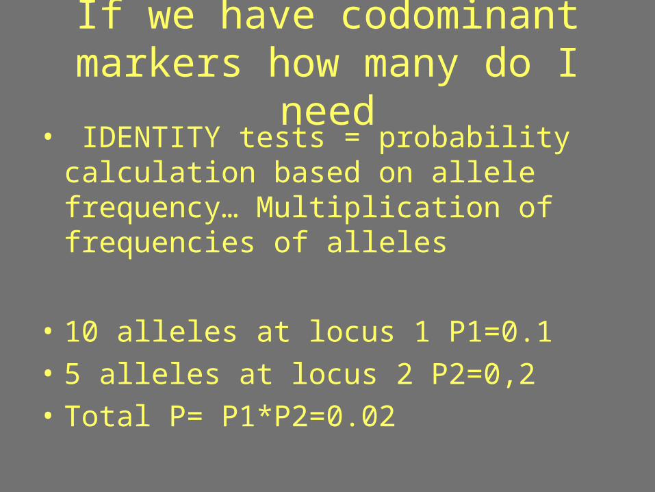
If we have codominant markers how many do I need
• IDENTITY tests = probability calculation based on allele frequency… Multiplication of frequencies of alleles
• 10 alleles at locus 1 P1=0.1
• 5 alleles at locus 2 P2=0,2
• Total P= P1*P2=0.02

Have we sampled enough?
• Resampling approaches
• Raraefaction curves
– A total of 30 polymorphic alleles– Our sample is either 10 or 20– Calculate whether each new sample is
characterized by new alleles

Saturation (rarefaction) curves
1 2 3 4 5 6 7 8 9 10 11 12 13 14 15 16 17 18 19 20
NoOf Newalleles

Dealing with dominant anonymous multilocus markers
• Need to use large numbers (linkage)
• Repeatability
• Graph distribution of distances
• Calculate distance using Jaccard’s similarity index

Jaccard’s
• Only 1-1 and 1-0 count, 0-0 do not count
1010011
1001011
1001000

Jaccard’s
• Only 1-1 and 1-0 count, 0-0 do not count
A: 1010011 AB= 0.60.4 (1-AB)
B: 1001011 BC=0.5 0.5
C: 1001000 AC=0.2 0.8

Now that we have distances….
• Plot their distribution (clonal vs. sexual)

Now that we have distances….
• Plot their distribution (clonal vs. sexual)
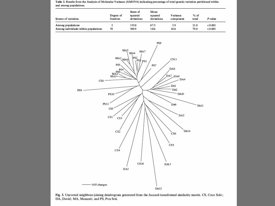
• Analysis: – Similarity (cluster analysis); a variety of
algorithms. Most common are NJ and UPGMA

Now that we have distances….
• Plot their distribution (clonal vs. sexual)
• Analysis: – Similarity (cluster analysis); a variety of
algorithms. Most common are NJ and UPGMA
– AMOVA; requires a priori grouping

Results: Jaccard similarity coefficients
0.3
0.90 0.92 0.94 0.96 0.98 1.00
00.10.2
0.40.50.60.7
Coefficient
Fre
quen
cy
P. nemorosa
P. pseudosyringae: U.S. and E.U.
0.3
Coefficient0.90 0.92 0.94 0.96 0.98 1.00
00.10.2
0.40.50.60.7
Fre
quen
cy

0.1
4175A
p72
p39
p91
1050
p7
2502
p51
2055.2
2146.1
5104
4083.1
2512
2510
2501
2500
2204
2201
2162.1
2155.3
2140.2
2140.1
2134.1
2059.2
2052.2
HCT4
MWT5
p114
p113
p61
p59
p52
p44
p38
p37
p13
p16
2059.4
p115
2156.1
HCT7
p106
P. nemorosa
P. ilicisP. pseudosyringae
Results: Results: P. nemorosaP. nemorosa

Results: Results: P. pseudosyringaeP. pseudosyringae
0.1
4175A2055.2p44
FC2D
FC2EGEROR4
FC1B
FCHHDFCHHCFC1A
p80
FAGGIO 2FAGGIO 1FCHHB
FCHHAFC2FFC2C
FC1FFC1DFC1Cp83
p40BU9715
p50
p94p92
p88p90
p56Bp45
p41
p72p84p85
p86p87p93p96
p39p118p97
p81p76p73p70
p69p62p55
p54HELA2HELA 1
P. nemorosaP. ilicis
P. pseudosyringae
= E.U. isolate
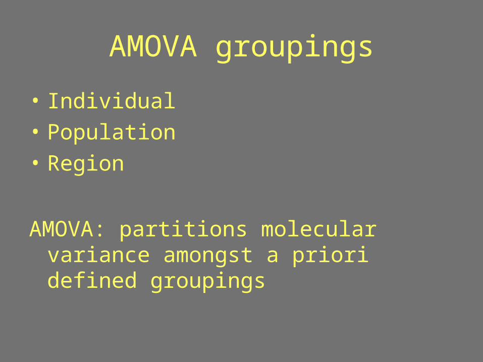
AMOVA groupings
• Individual
• Population
• Region
AMOVA: partitions molecular variance amongst a priori defined groupings

Example
• SPECIES X: 50%blue, 50% yellow

AMOVA: example
v
Scenario 1 Scenario 2
POP 1
POP 2v

Expectations for fungi
• Sexually reproducing fungi characterized by high percentage of variance explained by individual populations
• Amount of variance between populations and regions will depend on ability of organism to move, availability of host, and
• NOTE: if genotypes are not sensitive enough so you are calling “the same” things that are different you may get unreliable results like 100 variance within pops, none among pops

The “scale” of disease
• Dispersal gradients dependent on propagule size, resilience, ability to dessicate, NOTE: not linear
• Important interaction with environment, habitat, and niche availability. Examples: Heterobasidion in Western Alps, Matsutake mushrooms that offer example of habitat tracking
• Scale of dispersal (implicitely correlated to metapopulation structure)---
QuickTime™ and aTIFF (LZW) decompressor
are needed to see this picture.

RAPDS> not used often now
QuickTime™ and aTIFF (LZW) decompressor
are needed to see this picture.

QuickTime™ and aTIFF (LZW) decompressor
are needed to see this picture.
RAPD DATA W/O COSEGREGATING MARKERS


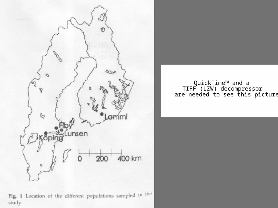
White mangroves:Corioloposis caperata
Coco Solo Mananti Ponsok DavidCoco Solo 0Mananti 237 0Ponsok 273 60 0David 307 89 113 0
Distances between study sites

Coriolopsis caperataCoriolopsis caperata on on Laguncularia racemosaLaguncularia racemosa
Forest fragmentation can lead to loss of gene flow among previously contiguous populations. The negative repercussions of such genetic isolation should most severely affect highly specialized organisms such as some plant-parasitic fungi.
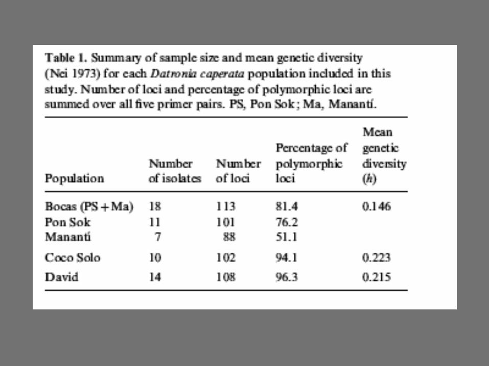
AFLP study on single spores
Site # of isolates # of loci % fixed alleles
Coco Solo 11 113 2.6
David 14 104 3.7
Bocas 18 92 15.04

Distances =PhiST between pairs ofpopulations. Above diagonal is the ProbabilityRandom distance > Observed distance (1000iterations).
Coco Solo Bocas David
Coco Solo 0.000 0.000 0.000
Bocas 0.2083 0.000 0.000
David 0.1109 0.2533 0.000


32
-0.2
-0.1
0
0.1
0.2
0.3
0.4
0.5
0.6
1 10 100 1000 10000 100000 1000000
Mean Geographical Distance (m)
Moran's
I
Spatial autocorrelation
Moran’s I (coefficient of departure from spatial randomness) correlates with distance up to Distribution of genotypes (6 microsatellite markers) in different populations of P.ramorum in California
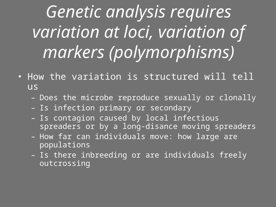
Genetic analysis requires variation at loci, variation of markers (polymorphisms)
• How the variation is structured will tell us– Does the microbe reproduce sexually or clonally– Is infection primary or secondary– Is contagion caused by local infectious spreaders or by a long-
disance moving spreaders– How far can individuals move: how large are populations– Is there inbreeding or are individuals freely outcrossing
CASE STUDY
A stand of adjacent trees is infected by a disease:
How can we determine the way trees are infected?
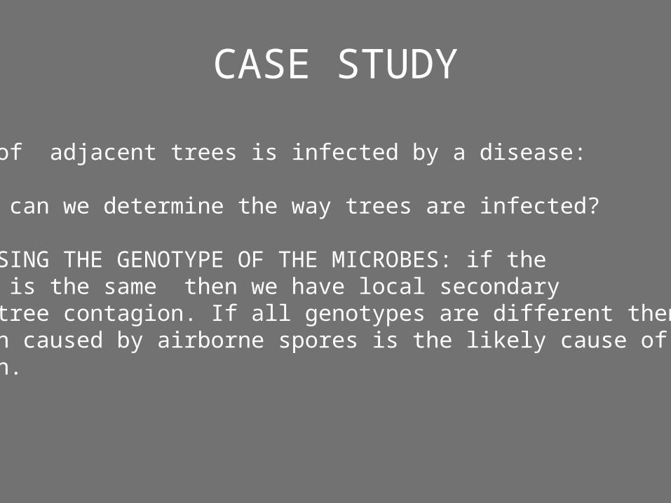
CASE STUDY
A stand of adjacent trees is infected by a disease:
How can we determine the way trees are infected?
BY ANALYSING THE GENOTYPE OF THE MICROBES: if the genotype is the same then we have local secondary tree-to-tree contagion. If all genotypes are different then primary infection caused by airborne spores is the likely cause of Contagion.

CASE STUDY
WE HAVE DETERMINED AIRBORNE SPORES (PRIMARY INFECTION ) IS THE MOST COMMON FORM OF INFECTION
QUESTION: Are the infectious spores produced by a localspreader, or is there a general airborne population of spores thatmay come from far away ?
HOW CAN WE ANSWER THIS QUESTION?

If spores are produced by a local spreader..
• Even if each tree is infected by different genotypes (each representing the result of meiosis like us here in this class)….these genotypes will be related
• HOW CAN WE DETERMINE IF THEY ARE RELATED?

HOW CAN WE DETERMINE IF THEY ARE RELATED?
• By using random genetic markers we find out the genetic similarity among these genotypes infecting adjacent trees is high
• If all spores are generated by one individual– They should have the same mitochondrial
genome– They should have one of two mating alleles

WE DETERMINE INFECTIOUS SPORES ARE NOT RELATED
• QUESTION: HOW FAR ARE THEY COMING FROM? ….or……
• HOW LARGE IS A POPULATION?Very important question: if we decide we want to wipe out
an infectious disease we need to wipe out at least the areas corresponding to the population size, otherwise we will achieve no result.

HOW TO DETERMINE WHETHER DIFFERENT SITES BELONG TO THE SAME POP
OR NOT?• Sample the sites and run the genetic markers
• If sites are very different:
– All individuals from each site will be in their own exclusive clade, if two sites are in the same clade maybe those two populations actually are linked (within reach)
– In AMOVA analysis, amount of genetic variance among populations will be significant (if organism is sexual portion of variance among individuals will also be significant)
– F statistics: Fst will be over ) 0.10 (suggesting sttong structuring)– There will be isolation by distance

Levels of Analyses
Individual
• identifying parents & offspring– very important in zoological circles – identify patterns of mating between individuals (polyandry, etc.)
In fungi, it is important to identify the "individual" -- determining clonal individuals from unique individuals that resulted from a single mating event.

Levels of Analyses cont…
• Families – looking at relatedness within colonies (ants, bees, etc.)
• Population – level of variation within a population. – Dispersal = indirectly estimate by calculating
migration– Conservation & Management = looking for
founder effects (little allelic variation), bottlenecks (reduction in population size leads to little allelic variation)
• Species – variation among species = what are the relationship between species.
• Family, Order, ETC. = higher level phylogenies

What is Population Genetics?
About microevolution (evolution of species)
The study of the change of allele frequencies,
genotype frequencies, and phenotype
frequencies

• Natural selection (adaptation)• Chance (random events)• Mutations• Climatic changes (population expansions and contractions)• …To provide an explanatory framework to describe the evolutionof species, organisms, and their genome, due to:Assumes that:• the same evolutionary forces acting within species(populations) should enable us to explain the differences we seebetween species• evolution leads to change in gene frequencies within populations
Goals of population genetics

Pathogen Population Genetics
• must constantly adapt to changing environmental conditions to survive– High genetic diversity = easily adapted– Low genetic diversity = difficult to adapt to changing
environmental conditions– important for determining evolutionary potential of a pathogen
• If we are to control a disease, must target a population rather than individual
• Exhibit a diverse array of reproductive strategies that impact population biology

Analytical Techniques
– Hardy-Weinberg Equilibrium • p2 + 2pq + q2 = 1• Departures from non-random mating
– F-Statistics• measures of genetic differentiation in populations
– Genetic Distances – degree of similarity between OTUs
• Nei’s• Reynolds• Jaccards• Cavalli-Sforza
– Tree Algorithms – visualization of similarity• UPGMA• Neighbor Joining

Allele Frequencies
• Allele frequencies (gene frequencies) = proportion of all alleles in an all individuals in the group in question which are a particular type
• Allele frequencies: p + q = 1
• Expected genotype frequencies: p2 + 2pq + q2

Evolutionary principles: Factors causing changes in genotype
frequency • Selection = variation in fitness; heritable• Mutation = change in DNA of genes• Migration = movement of genes across populations
– Vectors = Pollen, Spores
• Recombination = exchange of gene segments• Non-random Mating = mating between neighbors rather
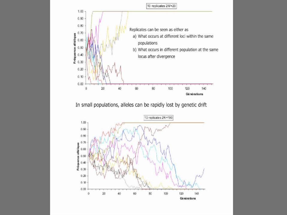
than by chance• Random Genetic Drift = if populations are small
enough, by chance, sampling will result in a different allele frequency from one generation to the next.

The smaller the sample, the greater the chance of deviation from an ideal population.
Genetic drift at small population sizes often occurs as a result of two situations: the bottleneck effect or the founder effect.

Founder Effects; typical of exotic diseases
• Establishment of a population by a few individuals can profoundly affect genetic variation– Consequences of Founder effects
• Fewer alleles• Fixed alleles• Modified allele frequencies compared to source pop• GREATER THAN EXPECTED DIFFERENCES AMONG POPULATIONS
BECAUSE POPULATIONS NOT IN EQUILIBRIUM (IF A BLONDE FOUNDS TOWN A AND A BRUNETTE FOUND TOWN B ANDF THERE IS NO MOVEMENT BETWEEN TOWNS, WE WILL ISTANTANEOUSLY OBSERVE POPULATION DIFFERENTIATION)

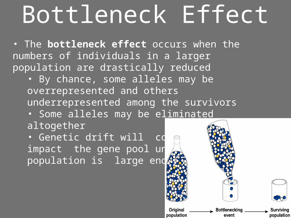
• The bottleneck effect occurs when the numbers of individuals in a larger population are drastically reduced
• By chance, some alleles may be overrepresented and others underrepresented among the survivors• Some alleles may be eliminated altogether• Genetic drift will continue to impact the gene pool until the population is large enough
Bottleneck Effect
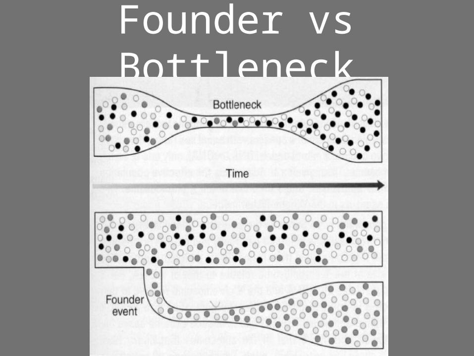
Founder vs Bottleneck

Northern Elephant Seal: Example of Bottleneck
Hunted down to 20 individuals in 1890’s
Population has recovered to over 30,000
No genetic diversity at 20 loci

Hardy Weinberg Equilibriumand F-Stats
• In general, requires co-dominant marker system• Codominant = expression of heterozygote
phenotypes that differ from either homozygote phenotype.
• AA, Aa, aa

Hardy-Weinberg Equilibrium
• Null Model = population is in HW Equilibrium– Useful– Often predicts genotype frequencies well

if only random mating occurs, then allele frequenciesremain unchanged over time.
After one generation of random-mating, genotype frequencies are given by
AA Aa aap2 2pq q2
p = freq (A)q = freq (a)
Hardy-Weinberg Theorem

• The possible range for an allele frequency or genotype frequency therefore lies between ( 0 – 1)
• with 0 meaning complete absence of that allele or genotype from the population (no individual in the population carries that allele or genotype)
• 1 means complete fixation of the allele or genotype (fixation means that every individual in the population is homozygous for the allele -- i.e., has the same genotype at that locus).
Expected Genotype Frequencies

1) diploid organism2) sexual reproduction3) Discrete generations (no overlap)4) mating occurs at random5) large population size (infinite)6) No migration (closed population)7) Mutations can be ignored8) No selection on alleles
ASSUMPTIONS
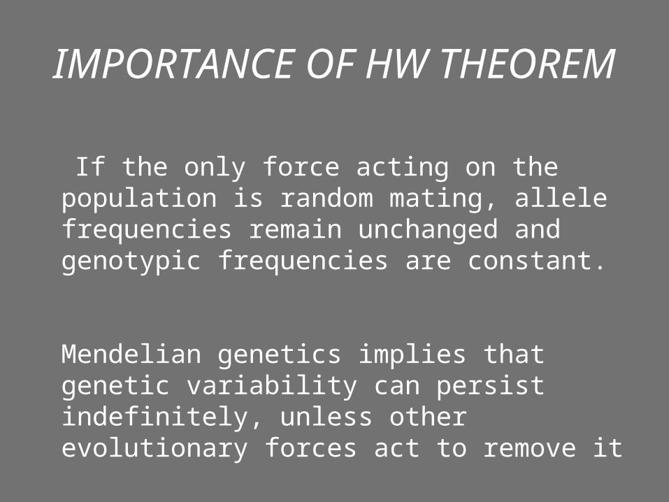
If the only force acting on the population is random mating, allele frequencies remain unchanged and genotypic frequencies are constant.
Mendelian genetics implies that genetic variability can persist indefinitely, unless other evolutionary forces act to remove it
IMPORTANCE OF HW THEOREM

Departures from HW Equilibrium
• Check Gene Diversity = Heterozygosity– If high gene diversity = different genetic sources due
to high levels of migration
• Inbreeding - mating system “leaky” or breaks down allowing mating between siblings
• Asexual reproduction = check for clones– Risk of over emphasizing particular individuals
• Restricted dispersal = local differentiation leads to non-random mating

Pop 1
Pop 2Pop 3
Pop 4
FST = 0.02FST = 0.30

Pop1 Pop2 Pop3
Sample size
20 20 20
AA 10 5 0
Aa 4 10 8
aa 6 5 12

Pop1 Pop2 Pop3
Freq
p (20 + 1/2*8)/40 = 0.60
(10+1/2*20)/40 = .50
(0+1/2*16)/40 = 0.20
q (12 + 1/2*8)/40 = 0.40
(10+1/2*20)/40 = .50
(24+1/2*16)/40 = 0.80

• Calculate HOBS
– Pop1: 4/20 = 0.20– Pop2: 10/20 = 0.50– Pop3: 8/20 = 0.40
• Calculate HEXP (2pq)– Pop1: 2*0.60*0.40 = 0.48– Pop2: 2*0.50*0.50 = 0.50– Pop3: 2*0.20*0.80 = 0.32
• Calculate F = (HEXP – HOBS)/ HEXP
• Pop1 = (0.48 – 0.20)/(0.48) = 0.583• Pop2 = (0.50 – 0.50)/(0.50) = 0.000• Pop3 = (0.32 – 0.40)/(0.32) = -0.250
Local Inbreeding Coefficient
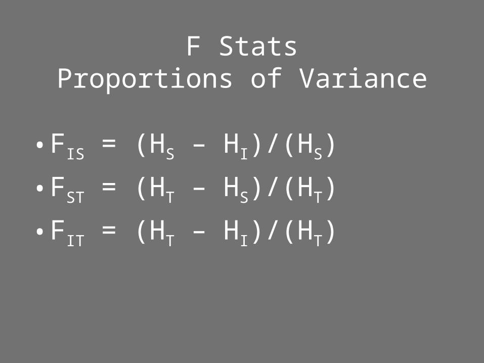
F StatsProportions of Variance
• FIS = (HS – HI)/(HS)
• FST = (HT – HS)/(HT)
• FIT = (HT – HI)/(HT)

Pop Hs HI p q HT FIS FST FIT
1 0.48 0.20 0.60 0.40
2 0.50 0.50 0.50 0.50
3 0.32 0.40 0.20 0.80
Mean
0.43 0.37 0.43 0.57 0.49 -0.14
0.12 0.24

Important point
• Fst values are significant or not depending on the organism you are studying or reading about:
– Fst =0.10 would be outrageous for humans, for fungi means modest substructuring

Rhizopogon vulgaris
Rhizopogon occidentalisHost islands within the California Northern ChannelIslands create fine-scale genetic structure in two sympatricspecies of the symbiotic ectomycorrhizal fungusRhizopogon

Rhizopogon sampling & study area
• Santa Rosa, Santa Cruz– R. occidentalis– R. vulgaris
• Overlapping ranges– Sympatric– Independent
evolutionary histories

BT
N E
W
Local Scale Population Structure
Rhizopogon occidentalis
FST = 0.26
FST = 0.33FST = 0.24
Grubisha LC, Bergemann SE, Bruns TDMolecular Ecology in press.
FST = 0.17
Populations are differentPopulations are similar
8-19 km
5 km


