
Pasi Suhonen
Radio Frequency Interference Measurements in WLAN Networks
Helsinki Metropolia University of Applied Sciences
Master of Engineering
Information Technology
Master’s Thesis
15 March 2019
PREFACE
Modern society depends on wireless communication transferring information between
machines and humans. Wireless networks, such as WLAN networks, usually function
without problems, but there can also be challenging difficulties. Most young network
engineers have the capability for solving problems in the data link layer and above.
This study has been done to evoke awareness of the first and most essential thing for
successful wireless data transfer, i.e. the proper functioning of the physical layer. Dur-
ing the course of study, I learned that even normal everyday household machines,
such as microwave ovens and Bluetooth device, can in the worst case cause serious
interferences for the WLAN network physical layer signal operating in the 2.4 GHz ISM
frequency band.
I have spent many hours and long nights to bring this study into a successful end. I
would like to thank my instructors B.Sc.(Eng.) Markku Hintsala for teaching me modern
spectrum analyzer technology and Principal Lecturer Matti Fischer for guiding me
through the thesis writing process. Special acknowledgements go to my wife Kirsikka
Suhonen and M.A.D.Sc.(Econ.) Marjukka Lehtinen for supporting and encouraging me
during all those challenging times while studying. This study has been a long journey
for me, but thanks to these remarkable people now it is successfully finished.
Hyvinkää, 15 March 2019 Pasi Suhonen

Author Title Number of Pages Date
Pasi Suhonen Radio frequency interference measurements in WLAN networks 86 pages + 2 appendices 15 March 2019
Degree Master of Engineering
Degree Programme Information Technology
Specialisation option Health Technology
Instructors
Markku Hintsala, Application Engineer Matti Fischer, Principal Lecturer
External radio frequency interference signals are causing malfunctions and disruptions to indoor and outdoor WLAN devices degrading their Quality of Service (QoS). This study aims to help hospitals to ensure that their WLAN networks function without interference. To address this issue, this study adds to the knowledge of how to detect and measure inter-ference signals from external sources and what kind of measurement equipment can be used for interference measurements. In practice, there were some challenges in data gath-ering in a hospital environment due to confidentiality and technical measurement test setup reasons. Instead of performing measurements in hospital premises, an experimental WLAN network was constructed in a sales office environment for interference and data bandwidth measurement purposes.
The study is divided in a theoretical framework and a practical part. The theoretical part focuses on explaining typical RF-interference signal characteristics and WLAN standards physical layer properties. The typical structure of hospital WLAN networks and properties of modern spectrum analyzer and measurement antennas were also described in theory. In the practical part of the study, a microwave oven and a Bluetooth loudspeaker were used as external interferer sources inside the experimental WLAN network. The frequency, pow-er level, RF-bandwidth of interference signals and WLAN network data bandwidth were measured with a spectrum analyzer and a network performance software tool. The results of this study shows that an external interference source, such as a microwave oven or a Bluetooth device can cause problems to the WLAN network physical layer signal, and in the worst case dramatically decrease networks quality of service and performance. A mod-ern real time spectrum analyzer in combination with a highly directive measurement anten-na are the most effective choice of measurement equipment for detecting and measuring wideband, narrowband and periodical spurious interference signals in the WLAN networks.
Keywords Interference, WLAN network, Spectrum analyzer
Abstract
Contents
Preface
Abstract
List of Abbreviations
List of Abbreviations
1 Introduction 1
1.1 Background of case company Rohde&Schwarz 2
1.2 Technology and business problem for RF interferences in WLAN networks 2
1.3 Research question, scope and structure of the study for RF interference measurements in WLAN networks 3
2 Method and material of study 4
2.1 Research design and approach 4
3 Existing knowledge of WLAN network technical environment 8
3.1 Characteristics of typical radio frequency Interference Signals 8
3.2 Typical interference sources on the WLAN network 12
3.3 Typical structure of hospital WLAN networks 16
3.4 An overview of 802.11 physical layer standards 20
3.5 Basic operating principles of measurement devices 24
3.5.1 Measurement antennas 24
3.5.2 Spectrum analyzer 35
4 RF-interference and data bandwidth measurements in office WLAN network 48
4.1 Description of test setup 48
4.2 Measurements for external RF-interference sources 55
4.2.1 Reference measurement for campus WLAN network 55
4.2.2 Interference measurement for microwave oven 61
4.2.3 Interference measurement for Bluetooth loudspeaker 65
4.3 Recording of WLAN network data bandwidth 69
4.3.1 Reference data bandwidth measurement 69
4.3.2 Data bandwidth measurement under external interference sources 72
4.4 Analysis of measured data 74
4.4.1 External RF-interference signals 74
4.4.2 WLAN network data bandwidth 77
5 Practical implications for hospital WLAN network environment 79
6 Proposed actions and suggestions 82
7 Conclusions 85
References 87
Appendices
Appendix 1. Spectrum analyzer measurement results for microwave oven RF-
interference signals in swept tuned and real time modes.
Appendix 2. Spectrum analyzer measurement results for Bluetooth loudspeaker RF-
interference signals in swept tuned and real time modes.
List of Abbreviations
ADC Analog to Digital Converter
ADSL Asymmetric Digital Subscriber Line
CSMA/CA Carrier Sense Multiple Access with Collision Avoidance
CW Continuous Wave
DANL Displayed Average Noise Level
dB Decibel
dBm Decibel milliwatt
DC Direct Current
DFS Dynamic Frequency Selection
DHCP Dynamic Host Configuration Protocol
DSSS Direct Sequence Spread Spectrum
DUT Device Under Test
EAP Extensible Authentication Protocol
EMF Electromagnetic Field
EMI Electro Magnetic Interference
E-Plane Plane which contains electric field vector for linearly polarized antenna
FFT Fast Fourier Transform
FHSS Frequency Hopping Spread Spectrum
FPGA Field Programmable Gate Array
HPBW Half Power Beamwidth
H-Plane Plane which contains magnetic field vector for linearly polarized antenna
IEEE Institute of Electrical and Electronics Engineers
IF Intermediate Frequency
IP Internet Protocol
IP2 Second Order Intercept Point
IP3 Third Order Intercept Point
ISM Industrial, Scientific and Medical
IT Information Technology
LAN Local Area Network
LCD Liquid Crystal Display
LHC Left Hand Circular Polarization of Incoming Signal E Vector
LNA Low Noise Amplifier
LO Local Oscillator
MAC Medium Access Control

MIMO Multiple Input Multiple Output
MU-MIMO Multi User Multiple Input Multiple Output
NIC Network Interface Card
OCXO Oven Controlled Crystal Oscillators
OSI Open Source Interconnection
PBX Private Branch Exchange
PDA Personal Digital Assistant
PLL Phase Locked Loop
PSK Pre Shared Key
QAM Quadrature Amplitude Modulation
QoS Quality of Service
R&D Research and Development
RAM Random Access Memory
RBW Resolution Bandwidth
RF Radio Frequency
RFI Radio Frequency Interference
RHC Right Hand Circular Polarization of Incoming Signal E Vector
SHI Second Harmonic Intercept
SSB Single Side Band
SSID Service Set Identifier
TCP Transmission Control Protocol
TCXO Temperature Compensated Crystal Oscillator
TKIP Temporal Key Integrity Protocol
TPC Transmit Power Control
UDP User Datagram Protocol
UNII Unlicensed National Information Infrastructure
UWB Ultra Wide Band
VBW Video Bandwidth
VLAN Virtual Local Area Network
VSWR Voltage Standing Wave Ratio
WAN Wide Area Network
WIPS Wireless Intrusion Prevention System
WLAN Wireless Local Area Network
WPA2 Wi-Fi Protected Access II
WPA2-AES Wi-Fi Protected Access II with Advanced Encryption Standard
1
1 Introduction
Over the past decade, the number of wireless transmitter devices has dramatically in-
creased in the world. Wireless technology has become a critical part of our daily lives
but, at the same time, radio frequency interference has become a real problem. Every
significant electronic device leaks radiation. Today's radio frequency spectrum is very
crowded. Almost every frequency is being shared by some other wireless device.
These signals are creating noise, such as interference with other nearby signals, and
causing disruptions for device and service functionality. Individual noise sources can
consist of, for example, normal household appliances, cell phones, poorly shielded
power lines or light systems. Locating an interference source, known as interference
hunting, will be a major issue for engineers and spectrum managers in the future.
Today, Wireless Local Area Networks (WLAN) are deployed in almost all public and
private facilities and buildings, and they allow users to access the Internet without be-
ing physically tied to a specific location. Electrically operated devices can cause inter-
ference in WLAN networks, and larger institutions, such as hospitals, can face truly
complex issues in relation to interference signals. Devices with built-in transmitters in-
clude wide range of medical and commercial wireless devises.
Network administrators often deploy WLAN networks without knowing that non-wireless
devices are also operating in the 2.4 GHz ISM band. For example, trace capture pro-
grams designed for Local Area Network (LAN) site surveys detect network traffic activi-
ty from data link layer and up (see figure 7). This means that they cannot detect any RF
interferences coming from non-wireless devices. [4] For a more complete picture of the
RF interference activity on the 2.4 GHz ISM band, network administrators also need to
consider the physical layer, which is the focus of this study. The functionality of the first
layer (physical layer) is an absolute necessity for the functionality of the rest of the lay-
ers.

2
1.1 Background of case company Rohde&Schwarz
The case company in this project is Rohde&Schwarz. It is a leading international com-
pany specialized in delivering products and services for commercial and government
customers in the field of wireless communication technology. The company was found-
ed in 1933 by two doctors Dr. Lothar Rohde and Dr. Hermann Schwarz, and the head-
quarters are located in Munich, Germany. Company revenue was over 2 billion euros in
fiscal year 2017/2018 and the worldwide number of employees is around 10,500. The
company is family-owned and self-financing. Headquarter is located in Munich. Produc-
tion factory plants are located in Memmingen (Germany), Teisnach (Germany) and
Vimperk (the Czech Republic).
1.2 Technology and business problem for RF interferences in WLAN networks
This study has been ordered by Rohde&Schwarz Finland Oy, one of the around 70
subsidiaries of the parent company Rohde&Schwarz GmbH&Co KG. The offices of the
Finnish subsidiary are located in Vantaa and Oulu. The number of local employees is
27, consisting of administration, technical support, service and sales professionals. The
product portfolio of Rohde&Schwarz Finland is exactly the same as that of the parent
company. Rohde&Schwarz Finland has identified the health services sector as a lucra-
tive business segment.
Radio frequency interference signals are causing malfunctions and disruptions to in-
door and outdoor WLAN devices and degrading their quality of service (QoS). It can be
difficult to find the interferer signals. Every interferer leaves a footprint that gives a hint
as to what type of interferer it is. When the network or data transfer is not operating as
it should, administrators typically purchase cheap measurement devices, which only
reveal a part of the real problem but do not provide a comprehensive picture of the 2.4
GHz ISM or 5 GHz frequency band interference activity. In a sense, such measurement
devices are basically only indicators. This means that the actual interference problem
remains unsolved.
3
The solution would be to acquire a more sophisticated device, but this is not sufficient
as such. The user must also know how to operate the device, how to interpret the
measurement results and to understand how the WLAN networks and measurement
devices work. This requires a willingness to invest in the device and to acquire exper-
tise on the device.
1.3 Research question, scope and structure of the study for RF interference meas-urements in WLAN networks
This study aims to help hospitals to ensure that their WLAN networks function without
interference. To address this issue, this study adds to the knowledge of how to detect
and measure interference signals from external sources. The precise objective of this
study is to identify and determine the characteristics of typical radio frequency interfer-
ence signals that are causing problems in the WLAN network physical layer and sug-
gest what kind of measurement equipment can be used for interference hunting. The
outcome of this study is a concrete proposal for
• how to measure, detect and identify interference signals from the WLAN network physical layer
• what kind of measurement equipment can be used for interference hunt-ing.
This thesis is divided into seven chapters. Chapter 1 outlines the introduction, objec-
tives, scope and structure of the study. Chapter 2 describes the methods and material
used in this study. Chapter 3 presents existing knowledge of technical environment.
The purpose of this chapter is to explain the characteristics of radio frequency interfer-
ence signals, WLAN network physical layer properties and characteristics, the typical
structure of hospital WLAN networks and description of most common measurements
devices used in interference hunting. Chapter 4 introduces practical interference
measurements in office environment. The focus in this chapter is on measurement test
setup, WLAN network physical layer interference measurement, WLAN network band-
width measurement and analysis of measured data. Chapter 5 provides practical impli-
cations for the hospital WLAN network environment. Chapter 6 provides a proposal for
RF interference measurement in the WLAN network physical layer and suggests what
kinds of measurement equipment to use in RF interference hunting. Chapter 7 summa-
rizes, evaluates and concludes the study.
4
2 Method and material of study
This chapter discusses in detail how the data for this research was collected, pro-
cessed and analyzed. The study is divided into two parts, theoretical and practical. The
theoretical part concentrates on collecting a systematic set of data around the subject.
The practical part consists of actual interference measurements in office environment.
State of the art measurement devices were used in order to create a high-quality and
traceable set of measurement data.
2.1 Research design and approach
As shown in figure 1, the study started with a theoretical framework, which was focus-
ing on collecting a systematic set of data around the subject. The data was collected
from technical white papers, articles, literature, application notes and field test reports
available in the internet, the university library and databases. The study continued to
measurement data collection and the analysis part, where practical interference and
WLAN network bandwidth measurements were conducted in business office environ-
ment and the measured data was analyzed. Based on the analyzed data, a literature
outcome was created. It contains a proposal on how to measure, detect and identify
interference signals from the WLAN physical layer and suggests what kind of meas-
urement equipment can be used for interference hunting.

5
Figure 1. Research design of this study
The first step of the study focused on collecting relevant literature for the theoretical
framework. The second step started with a literature review that describes characteris-
tics of typical interfering signals and properties and characteristics of the WLAN physi-
cal layer. The third step explored the structure of hospital WLAN networks, functionali-
ties and properties of modern spectrum analyzers and measurement antennas in order
to be able to fully exploit the technical properties of the measurement device. The
fourth step focused on practical WLAN physical layer interference signal measure-
ments coming from typically used devices that operate at the same 2.4 GHz ISM band
as WLAN access points.
Interference signal characteristics of a microwave oven and a Bluetooth loudspeaker
were verified and their impact on the WLAN link data traffic bandwidth was studied.
These two test devices were selected because they are easily available and widely
used. In the fifth step, the properties and characteristics of measured interference sig-
nals and their impact on the WLAN link data traffic bandwidth was analyzed. The sixth
step created a literature outcome that was based on the analyzed data. An outcome
proposed how to measure, detect and identify interference signals from the WLAN
physical layer and suggest what kind of measurement equipment can be effectively
used for interference hunting.
6
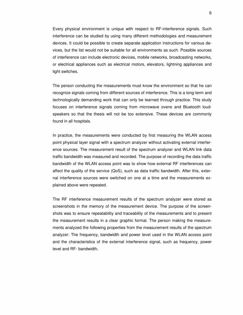
Every physical environment is unique with respect to RF-interference signals. Such
interference can be studied by using many different methodologies and measurement
devices. It could be possible to create separate application instructions for various de-
vices, but the list would not be suitable for all environments as such. Possible sources
of interference can include electronic devices, mobile networks, broadcasting networks,
or electrical appliances such as electrical motors, elevators, lightning appliances and
light switches.
The person conducting the measurements must know the environment so that he can
recognize signals coming from different sources of interference. This is a long-term and
technologically demanding work that can only be learned through practice. This study
focuses on interference signals coming from microwave ovens and Bluetooth loud-
speakers so that the thesis will not be too extensive. These devices are commonly
found in all hospitals.
In practice, the measurements were conducted by first measuring the WLAN access
point physical layer signal with a spectrum analyzer without activating external interfer-
ence sources. The measurement result of the spectrum analyzer and WLAN link data
traffic bandwidth was measured and recorded. The purpose of recording the data traffic
bandwidth of the WLAN access point was to show how external RF interferences can
affect the quality of the service (QoS), such as data traffic bandwidth. After this, exter-
nal interference sources were switched on one at a time and the measurements ex-
plained above were repeated.
The RF interference measurement results of the spectrum analyzer were stored as
screenshots in the memory of the measurement device. The purpose of the screen-
shots was to ensure repeatability and traceability of the measurements and to present
the measurement results in a clear graphic format. The person making the measure-
ments analyzed the following properties from the measurement results of the spectrum
analyzer: The frequency, bandwidth and power level used in the WLAN access point
and the characteristics of the external interference signal, such as frequency, power
level and RF- bandwidth.

7
The IP-data traffic bandwidth used in the WLAN network was measured with Internet
Protocol (IP) network bandwidth analyzing tool jPerf [11]. Test measurement results
were entered into excel sheet graphical chart presented in this thesis.
The person conducting the measurements of interference signals must have thorough
understanding of the following:
• What kind of physical environment measurements are performed
• What is the typical structure of the WLAN networks
• What are the basic properties of expected interference signals
• Which measurement devices are suitable for interference hunting
• How to operate the measurement devices
• How to analyze, store and interpret the measurement results
For the time being, it is not financially reasonable to use artificial intelligence in interfer-
ence measurements due to high costs. A portable spectrum analyzer costs approxi-
mately 5,000 euros while it will take hundreds of thousands of euros to develop artificial
intelligence for this purpose.
The measurement results and theoretical considerations can be universally applied in
numerous environments. While the focus of this study is on hospitals, there were some
practical challenges that posed a problem to data gathering in a hospital environment:
First, due to confidential requirements, the data gathered from the hospitals should be
kept confidential. However this thesis will be made publicly available. Secondly, in the
practical measurement phase, a microwave oven and a Bluetooth loudspeaker were
set as interferer sources. In the worst case, interferences coming out of them could
have disrupted the functionality and data traffic in the entire WLAN access point.
For these reasons, the practical measurement data for this study was collected from a
corresponding environment, i.e. normal office environment after business hours. It was
in theory possible that the power level of interference signals from the measured devic-
es is so low that no interference signals could be detected. However, in practice, inter-
ference signals were detected from both measured devices.

8
3 Existing knowledge of WLAN network technical environment
The following chapters provide a brief introduction into common types of Radio Fre-
quency Interference (RFI) and Electro Magnetic Interference (EMI) signals, how they
appear in the WLAN network physical layer, and how they are commonly character-
ized. Basic information from the typical structure of hospital WLAN networks, an over-
view of the 802.11 physical layer signal and basic operating principles of measurement
devices are also included.
3.1 Characteristics of typical radio frequency Interference Signals
Fundamentally, radio frequency interference is associated with degrading device per-
formance and quality of service (QoS). It usually means that the interference signal is
impacting a system or device causing it to work outside its normal technical parame-
ters. There are a few basic types of radio frequency interferences that could cause
problems for wireless devices. Interference signals are of certain type and are present
in various forms. This chapter presents typical types of interference signals that are
relevant for this study.
The first interference type is co-channel interference, which is basically crosstalk from
other radio transmitters using the same frequency. It can be generated, for example, by
cellular mobile networks, poor weather conditions, bad frequency planning or an overly
crowded radio spectrum. [6]. Figure 2 shows the generic picture of co-channel interfer-
ence situation, where different wireless devices are operating in the same radio chan-
nel.
Figure 2. Co-channel interference in 802.11n Access Point. [9]

9
Wireless devices such as laptops, tablets and smart phones are operating in the same
channels as WLAN access points. As shown in figure 2, the RF-power levels of differ-
ent devices may vary depending on the device in use. All devices working on the same
channel have to manage their timing and take turns in operation. This usually results in
degraded QoS.
The second interference type is adjacent channel interference, which is caused by ir-
relevant power coming from a transmitter in an adjacent radio channel. Typically, it is
generated by inadequate filtering of interfering modulation products in wireless sys-
tems, bad tuning or poor frequency control. [6]. Figure 3 shows a generic picture of
adjacent channel interference where different WLAN access points are operating in
adjacent overlapping radio channels.
Figure 3. Adjacent channel overlapping of separate WLAN access point channels. [9]
As shown in figure 3, wireless devices using overlapped channels could be transmitting
simultaneously. This may cause wireless signal collisions and lead to degraded QoS.
The third interference type is impulse noise, which could be created whenever a flow of
electricity is abruptly started or stopped. Many items can create impulse noise, such as
electrical motors, bakery ovens, welding equipment, light dimmers and power lines that
may arc and spark [6]. Figure 4 shows an example from the Electromagnetic Field
(EMF) measurement taken in the presence of normal household appliance interference
signals.

10
Figure 4. The frequency spectrum of impulse noise measurement. [12]
Interference signals coming from household appliances may cause impulse noise sig-
nals effecting a wideband of frequencies as shown in figure 4. The voltage and power
levels of interference signals vary in amplitude in respect of different frequencies. An
interfering noise signal can also be coming from a defective electronic device or it could
be caused by natural sources of interference, such as lightning and the sun.
The fourth interference type is Intermodulation (IM), which is one of the most common
and challenging types of interference problems in electronics. Intermodulation distortion
(IMD) is caused when two signals are combined in such a way, that they create inter-
modulation product signals at various combinations of two original frequencies. They
are usually created when two or more signals are interacting in a non-linear device
using active components, such as amplifiers and mixers.
Intermodulation distortion will produce additional unwanted signals and usually lead to
interference problems, which is hard to locate and measure without proper test equip-
ment. [6]. Figure 5 shows the order of different intermodulation products and their fre-
quency components generated by IMD distortion.

11
Figure 5. The order of different intermodulation products and their frequencies. [13]
As shown in figure 5, different frequency spectral components are caused by the mix-
ing of two or more fundamental frequency tones (f1 and f2) and their harmonics. Pas-
sive intermodulation (PIM) usually occurs in passive devices, such as cables, antennas
and connectors that are subject to two or more high power level signals. Passive inter-
modulation is usually created when two or more high power signals are mixed with de-
vice non-linearities, such as loose and corroded connectors. Passive intermodulation
can be a severe problem when both high power transmit and receiver signal paths are
shared by the same system. If PIM interference find its way to the receiver path, it is
very difficult to filter away. [7]
The fifth interference type is emissions such as out-of-band emissions and spurious
emission. They are caused by transmitters generating RF-signals that are outside their
intended transmission bandwidth. Out-of-band emissions could be caused by distortion
in the modulator or consists of broadband noise generated by the transmitter oscillators
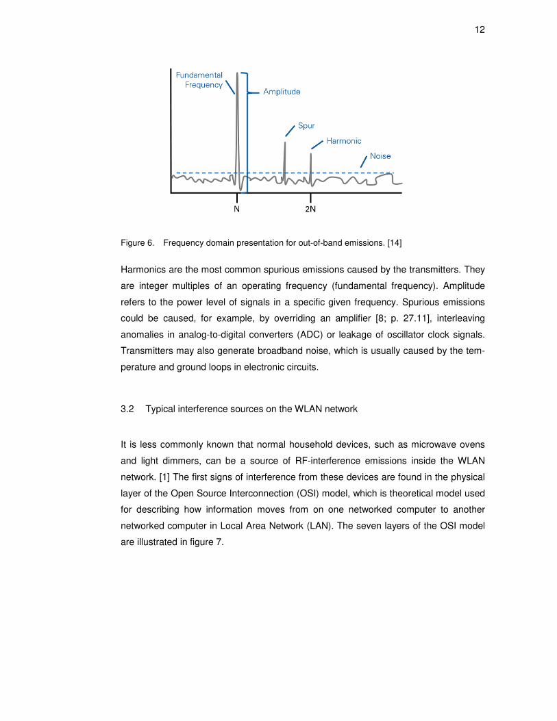
circuits that is added to the intended signal. Figure 6 shows a generic picture of funda-
mental, spurious, harmonic and noise level frequency components.
12
Figure 6. Frequency domain presentation for out-of-band emissions. [14]
Harmonics are the most common spurious emissions caused by the transmitters. They
are integer multiples of an operating frequency (fundamental frequency). Amplitude
refers to the power level of signals in a specific given frequency. Spurious emissions
could be caused, for example, by overriding an amplifier [8; p. 27.11], interleaving
anomalies in analog-to-digital converters (ADC) or leakage of oscillator clock signals.
Transmitters may also generate broadband noise, which is usually caused by the tem-
perature and ground loops in electronic circuits.
3.2 Typical interference sources on the WLAN network
It is less commonly known that normal household devices, such as microwave ovens
and light dimmers, can be a source of RF-interference emissions inside the WLAN
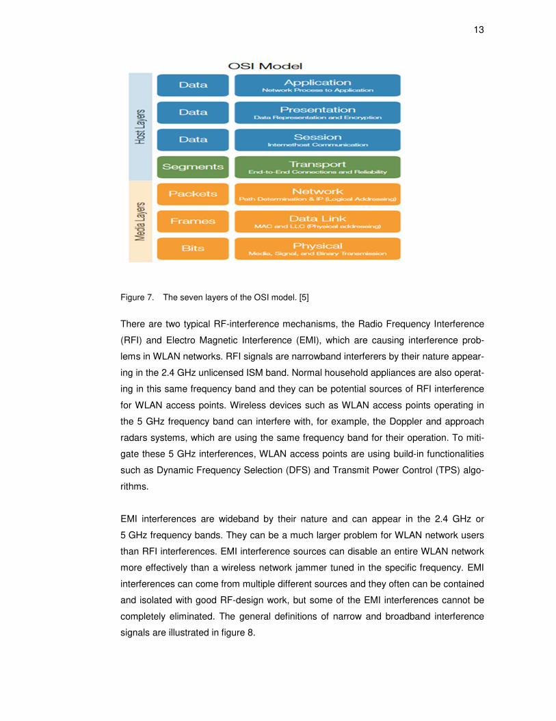
network. [1] The first signs of interference from these devices are found in the physical
layer of the Open Source Interconnection (OSI) model, which is theoretical model used
for describing how information moves from on one networked computer to another
networked computer in Local Area Network (LAN). The seven layers of the OSI model
are illustrated in figure 7.
13
Figure 7. The seven layers of the OSI model. [5]
There are two typical RF-interference mechanisms, the Radio Frequency Interference
(RFI) and Electro Magnetic Interference (EMI), which are causing interference prob-
lems in WLAN networks. RFI signals are narrowband interferers by their nature appear-
ing in the 2.4 GHz unlicensed ISM band. Normal household appliances are also operat-
ing in this same frequency band and they can be potential sources of RFI interference
for WLAN access points. Wireless devices such as WLAN access points operating in
the 5 GHz frequency band can interfere with, for example, the Doppler and approach
radars systems, which are using the same frequency band for their operation. To miti-
gate these 5 GHz interferences, WLAN access points are using build-in functionalities
such as Dynamic Frequency Selection (DFS) and Transmit Power Control (TPS) algo-
rithms.
EMI interferences are wideband by their nature and can appear in the 2.4 GHz or
5 GHz frequency bands. They can be a much larger problem for WLAN network users
than RFI interferences. EMI interference sources can disable an entire WLAN network
more effectively than a wireless network jammer tuned in the specific frequency. EMI
interferences can come from multiple different sources and they often can be contained
and isolated with good RF-design work, but some of the EMI interferences cannot be
completely eliminated. The general definitions of narrow and broadband interference
signals are illustrated in figure 8.

14
Figure 8. Generic presentation of narrow and broadband interference signals. [10]
The classification between narrow and broadband signals is defined by the occupied
frequency spectrum in relation to the measurement receiver Intermediate Frequency
(IF) stage resolution bandwidth (RBW). As shown in figure 8, the left picture presents
the definition of broadband interference signals and the right picture narrowband inter-
ference signals. The colored trace indicates the measurement device RBW filter band-
width. If the interference signal fits completely inside the RBW filter bandwidth, it is de-
fined as narrowband interference signal. If interference signals are detected outside the
RBW filter, the bandwidth is defined as broadband interference signal. Continuous
wave (CW) signals are classified as a special form of narrowband interference signals,
since they consist of only one narrow spectral line.
Typical WLAN network RFI and EMI interference sources and their basic interference
characteristics are listed below.
• Analog cordless phones are typically operating in the 2.4 GHz ISM fre-quency band. They are using narrow band transmission, which only dis-turbs the narrow bandwidth of spectrum in use. When they are placed in close proximity of the WLAN access points, they can cause really severe interference problems. [4; p.6]
• Wireless Baby Monitors, both analog and digital, are operating in the 2.4 GHz ISM band. When they are turned on, they will compete for bandwidth with the WLAN access points and can cause performance degradation and wideband RF interference problems, especially when they are placed in close proximity of access points. [4; p.8]
• Bluetooth technology devices are operating in the 2.4 GHz frequency band. Bluetooth devices are based on the Frequency Hopping Spread Spectrum (FHSS) modulation technique, and thus they hop across all channels in the entire 2.4 GHz frequency band in a random manner.
15
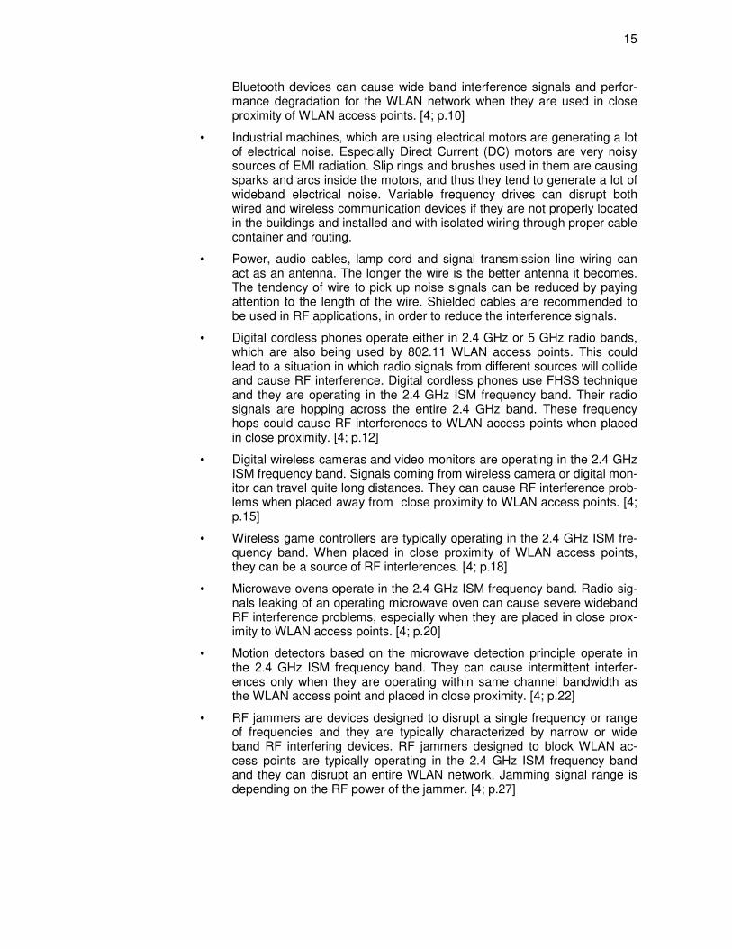
Bluetooth devices can cause wide band interference signals and perfor-mance degradation for the WLAN network when they are used in close proximity of WLAN access points. [4; p.10]
• Industrial machines, which are using electrical motors are generating a lot of electrical noise. Especially Direct Current (DC) motors are very noisy sources of EMI radiation. Slip rings and brushes used in them are causing sparks and arcs inside the motors, and thus they tend to generate a lot of wideband electrical noise. Variable frequency drives can disrupt both wired and wireless communication devices if they are not properly located in the buildings and installed and with isolated wiring through proper cable container and routing.
• Power, audio cables, lamp cord and signal transmission line wiring can act as an antenna. The longer the wire is the better antenna it becomes. The tendency of wire to pick up noise signals can be reduced by paying attention to the length of the wire. Shielded cables are recommended to be used in RF applications, in order to reduce the interference signals.
• Digital cordless phones operate either in 2.4 GHz or 5 GHz radio bands, which are also being used by 802.11 WLAN access points. This could lead to a situation in which radio signals from different sources will collide and cause RF interference. Digital cordless phones use FHSS technique and they are operating in the 2.4 GHz ISM frequency band. Their radio signals are hopping across the entire 2.4 GHz band. These frequency hops could cause RF interferences to WLAN access points when placed in close proximity. [4; p.12]
• Digital wireless cameras and video monitors are operating in the 2.4 GHz ISM frequency band. Signals coming from wireless camera or digital mon-itor can travel quite long distances. They can cause RF interference prob-lems when placed away from close proximity to WLAN access points. [4; p.15]
• Wireless game controllers are typically operating in the 2.4 GHz ISM fre-quency band. When placed in close proximity of WLAN access points, they can be a source of RF interferences. [4; p.18]
• Microwave ovens operate in the 2.4 GHz ISM frequency band. Radio sig-nals leaking of an operating microwave oven can cause severe wideband RF interference problems, especially when they are placed in close prox-imity to WLAN access points. [4; p.20]
• Motion detectors based on the microwave detection principle operate in the 2.4 GHz ISM frequency band. They can cause intermittent interfer-ences only when they are operating within same channel bandwidth as the WLAN access point and placed in close proximity. [4; p.22]
• RF jammers are devices designed to disrupt a single frequency or range of frequencies and they are typically characterized by narrow or wide band RF interfering devices. RF jammers designed to block WLAN ac-cess points are typically operating in the 2.4 GHz ISM frequency band and they can disrupt an entire WLAN network. Jamming signal range is depending on the RF power of the jammer. [4; p.27]

16
• ZiBee devices are low power, low cost and short range wireless devices. They are designed to operate in the 860 MHz, 915 MHz or 2.4 GHz fre-quency band using Direct Sequence Spread Spectrum (DSSS) modula-tion. The bandwidth of 2.4 GHz ZigBee network devices is fixed to 3 MHz. If ZibBee network happens to operate in same channel with the WLAN access point, chances for interferences are high, otherwise the interfer-ence effect from these low power ZigBee devices are low. [4; p.31]
• Remote controlled toys are typically using FHSS or DSSS modulation and they are operating in both 2.4 GHz ISM or 5 GHz frequency bands. They can cause severe RF interferences for WLAN access points operating in same frequencies. The actual severity level of interferences is depending on the range, relative signal levels and amount of data being transmitted by each devise wireless device. [4; p.33]
3.3 Typical structure of hospital WLAN networks
Hospital WLAN networks are using the Institute of Electrical and Electronics Engineers
(IEEE) 802.11 protocol and they operate in unlicensed 2.4 GHz Industrial, Scientific
and Medical (ISM) and 5 GHz Radio Frequency (RF) bands not only for regular internet
access but also for sensitive patient data transfer. [2] To access the internet, computing
devices and medical devices need to connect to hospital WLAN networks. Applications
running in medical devices cannot handle disruptions in network connectivity. A disrup-
tion of even milliseconds can cause a failure in critical patient data transmission. [3]
Devices such as general purpose WLAN clients, embedded WLAN monitoring systems
and asset tracking equipment are typically used in the hospital WLAN network. Fig-
ure 9 shows most commonly deployed devices and services used in a modern multi-
purpose medical WLAN network. [15; p.18]

17
Figure 9. Commonly deployed devices and services, used in modern medical networks. [15; p.18]
Many hospital organizations today are using the 802.11n based WLAN platform for
simultaneous support of all applications. The trend nowadays is that instead of having
many parallel WLAN networks for guest access and internal communication, all net-
work traffic is combined into a single pipe using a cost-effective and bandwidth-efficient
connection towards the Internet. [15; p.18]
Personal computers such as computers on wheels, desktop PCs, laptops and tablets
are using WLAN network access while mobile. Desktop PCs and computers on wheels
are normally used for accessing patient records, medical orders and hospital internal
servers. They should be configured to use Wi-Fi Protected Access II (WPA2) enterprise
security protocol with individual user log on credentials and support for voice and video
traffic. Personal Digital Assistant (PDA) computers and smart phones usually operate
in cellular network, but they are also capable of connecting to organizations’ WLAN
network and Private Branch Exchange (PBX) over the WLAN connection. WLAN net-
work parameters should be configured in such a way that they support maximum bat-
tery life for smartphone and PDA devices. [15; p.19]
Single mode Wi-Fi phones and voice communicator badges are normally used by clini-
cians who are working outside their usual office desk. Single mode phones are used as
cordless phones operating over the WLAN network. Voice communicator badges pro-
vide hands free voice recording and speech recognition for voice command and dialing.
18
Single mode Wi-Fi phones are typically using WPA2 with Pre Shared Key (PSK) au-
thentication protocol. Therefore proper firewall policies limiting access and protocol use
should be added to the network for enhancing network security. It is important to en-
sure seamless WLAN coverage in all areas where voice over WLAN services are de-
ployed. [15; p.19]
Wi-Fi locating tags are special RF devices optimized for low-cost, small size and long
battery life. Tags are attached to mobile devices, such as infusion pumps and wheel
chairs, in order to track their position and raise an alarm if equipment leaves a building
without proper authorization. With an asset tracking system, clinicians can track devic-
es in real time from a separate screen. When this system is used in the hospital, it is
important to ensure that there is a sufficient number of WLAN access points deployed
in the areas where asset tracking is performed. The system uses triangulation tech-
nique for locating Wi-Fi tags, which requires that at least three access points detect the
transmission from the tags. [15; p.20]
Medical devices, such as patient monitoring systems, provide continuous tracking of
critical physiological parameters for patient care. WLAN networks provide connectivity
between central nursing stations and moving patients. Patient monitors share the same
wireless multipurpose 802.11n network with other hospital applications and they send
alarms set to trigger after a small number of missed messages. Therefore, it is im-
portant to deliver traffic from patient monitors via network without data loss. [15; p.20]
In hospitals, the highest concentration of people is in public areas, such as cafeterias,
waiting rooms and atriums. These areas have a high number of users generating most
of the WLAN network traffic. While these areas are crowded by many users, they are
not difficult to cover with an interference-free WLAN network solution. The most chal-
lenging areas from the interference point of view are for example x-ray rooms, which
are encased with lead walls as a regulated safety precaution. The purpose of the lead
lining is to protect people from hazardous ionizing X-ray radiation. On the other hand,
lead walls are creating interference to clinical and medical wireless devices such as
patient monitors and WLAN access points. [16; p.4]
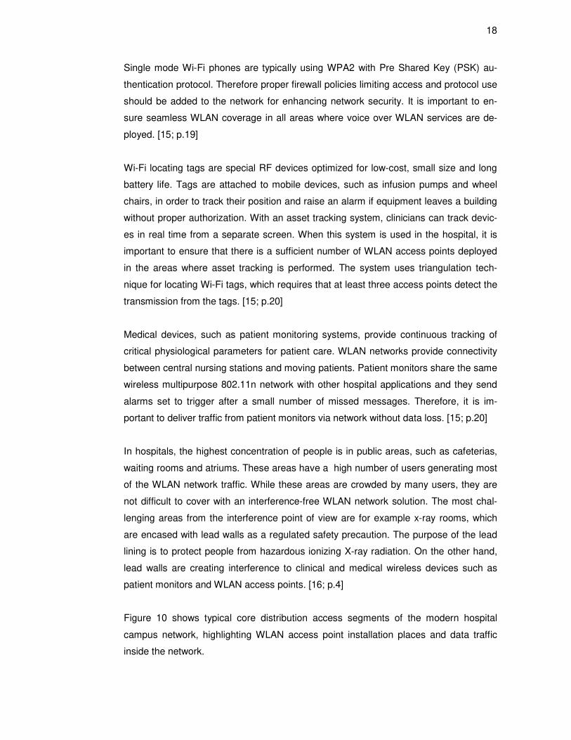
Figure 10 shows typical core distribution access segments of the modern hospital
campus network, highlighting WLAN access point installation places and data traffic
inside the network.
19
Figure 10. Typical healthcare campus network topology. [15; p.20]
Mobility controllers are positioned as required by data traffic patterns. A network man-
agement plane used for network monitoring, alarm generation and device configuration
purposes is typically using management software suite, which is connected over Local
Area Network (LAN) or Wide Area Network (WAN) to all mobility controllers in the net-
work. A control plane for handling RF coordination, handover between mobility control-
lers and access points and Wireless Intrusion Prevention System (WIPS) is set up as a
secure network of connections between mobility controllers. This allows fast handover
between access points homed to different mobility controllers. [15; p.21]
The traffic between mobility controllers and access points is using secure tunnels.
Hospital campus mobility controllers are usually positioned in separate data centers
with high bandwidth data links and high capacity LAN switches. In case of low data
bandwidth and network capacity are needed, mobility controllers can be placed closer
to distribution layer switches in order to minimize network traffic between the data cen-
ter and the hospital building. [15; p.21]

20
3.4 An overview of 802.11 physical layer standards
This chapter provides basic information of the existing 802.11 physical layer standards
in 2.4 GHz ISM and 5 GHz frequency bands. The most important information from the
interference measurement point of view is included. Detailed information, such as the
physical layer frame structure, packet formats, modulation scheme parameters or error
correction techniques are not part of the overall scope of this study. An overview of
IEEE 802.11 physical layer standards is shown in table 1 below.
Table 1. IEEE 802.11 physical layer standards. [19]
Radio frequencies used by different versions of 802.11 standards vary between differ-
ent countries. Basic standard 802.11 specifies maximum data rates up to 2 Mbit/s. It is
using the 2.4 GHz frequency band, 20 MHz bandwidth and DSSS or FHSS modulation
techniques. Version 802.11b was designed to increase the maximum data rate to 11
Mbit/s. It is using the 2.4 GHz frequency band, 20 MHz bandwidth and DSSS modula-
tion technique. [2; p.4]
Standard version 802.11a is operating in the 5 GHz band. It is using the Orthogonal
Frequency Division Multiplexing (OFDM) modulation technique, consisting of 52 sepa-
rate subcarriers occupying the 20 MHz bandwidth. The maximum data rate of 54 Mbit/s
can be achieved in theory, but in practice a throughput of approximately 20 Mbit/s is
achieved in real live networks due to physical environment restrictions. Version
802.11g operates in the 2.4 GHz frequency band, using the 20 MHz bandwidth and
OFDM modulation technique. A maximum data rate of 54 Mbit/s can be achieved. [2;
p.6]

21
Version 802.11n includes many improvements for WLAN range, throughput and relia-
bility. Advanced OFDM modulation technique and signal processing have been added
in order to use multiple antennas and wider channel bandwidths. 802.11n compatible
devices can be operated both in 2.4 GHz or 5 GHz frequency bands. The Multiple Input
Multiple Output (MIMO) antenna technique and 40 MHz bandwidth are defined in the
standard. 802.11n devices are able to transmit and receive simultaneously through
multiple antennas ranging from 1 x 1 to 4 x 4 configurations providing maximum data
rates 54 Mbit/s–600 Mbit/s. [2; p.6]
Version 802.11ac is providing high data throughput in the 5 GHz frequency band. Wid-
er bandwidth up to 160 MHz, Multi User Multiple Input Multiple Output (MU-MIMO),
using up to 8 spatial streams and high density 256 Quadrature Amplitude Modulation
(256-QAM) OFDM modulation techniques are used to achieve maximum data rate of
6.93 Gbit/s. [20; p.7]
Version 802.11ax is design to operate in 2.4 GHz or 5 GHz frequency bands. The main
goal is to improve user experience and network performance by providing at least four
times improvement into average data throughput per WLAN station reaching up to
maximum 10.53 Gbit/s. 802.11ax is supporting MU-MIMO in the uplink as well as in
downlink directions, using up to 8 spatial streams. A high density OFDM modulation
scheme up to 1024-QAM can be used. [21; p.7]
All WLAN devices are supporting 2.4 GHz ISM frequency band, thus it is used almost
in all WLAN networks. The 2.4 GHz frequency band is more crowded and sensitive to
interferences compared to the 5 GHz frequency band. The total occupied bandwidth for
2.4 GHz frequency band is 85 MHz, covering frequencies 2.400 - 2.485 GHz. The
bandwidth for a single channel is 5 MHz wide. In practice, several channels are cou-
pled together in order to increase maximum data rate in the transmission channels.
The 802.11 and 802.11b standards are using the 22 MHz wide bandwidth, in 802.11g
and 802.11n standards the channel bandwidth is increased to 20 MHz, because a
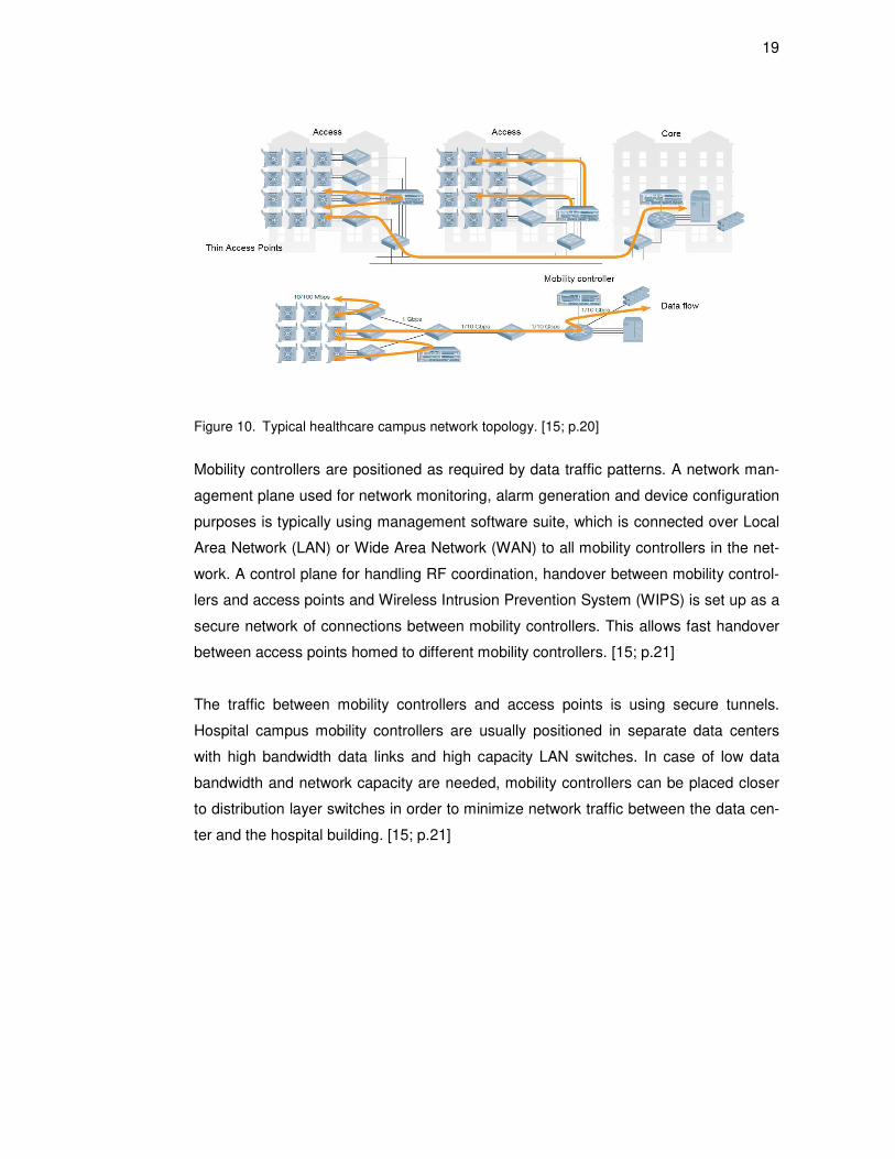
more effective OFDM modulation technique is in use. Channel numbers and their cen-
ter frequencies for the 2.4 GHz frequency band are shown in figure 11 below.
22
Figure 11. Channel numbers in 2.4 GHz frequency band and their center frequencies. [2; p.10]
Europe and most other parts in the world use 13 channels, Japan is using 14 channels
and the United States 11. Most of the WLAN radios are built to listen the 22 MHz wide
bandwidth and if they detect traffic in same channel, they do not transmit data before
the channel is free. If two WLAN hotspots are configured to run in adjacent channels,
for example in channels 1 and 2, they take turns in transmitting and as a consequence
they may end up delivering only half of the maximum available data rate capacity per
WLAN hotspot. Channels 1, 6 and 11 are not overlapping with each other. As a general
rule of the WLAN network design, hotspots should be configured to use non-
overlapping channels such as 1, 6 and 11, in order to reach maximum data rates in the
network.
The maximum allowed transmitting power for a WLAN device operating in the 2.4 GHz
frequency band is 100 mW (20 dBm). The wavelength in the 2.4 GHz frequency band
is two times longer than the 5 GHz frequency band. In practice, this means that the 2.4
GHz signal gets less attenuated in free space or building structures such as walls, al-
lowing stronger signal strength and wider network coverage areas using a small num-
ber of WLAN hotspots in the network. On the other hand, the 2.4 GHz frequency band
is more prone to external interference signals coming from commercial and industrial
devices operating in the same frequency band and it is more crowded than the 5 GHz
band.
The 5 GHz frequency band has more available channels and they are less error-prone
for external interference signals. Maximum data rates can be achieved by increasing
the channel bandwidth by coupling several channels together. The 5 GHz band was
first defined in standard 802.11a, but during the time it was released it was too expen-
sive and not commonly used. The 802.11n standard made it possible to choose be-
tween 2.4 GHz and 5 GHz bands, increasing the number of 5 GHz devices. The chan-
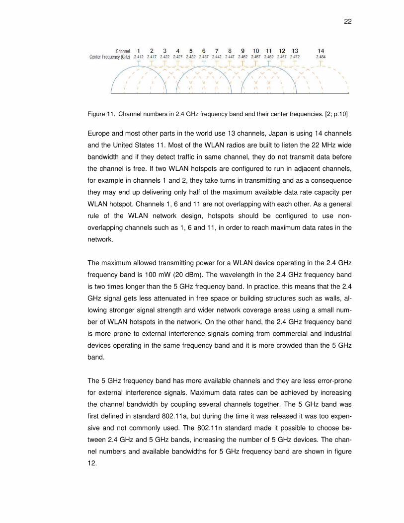
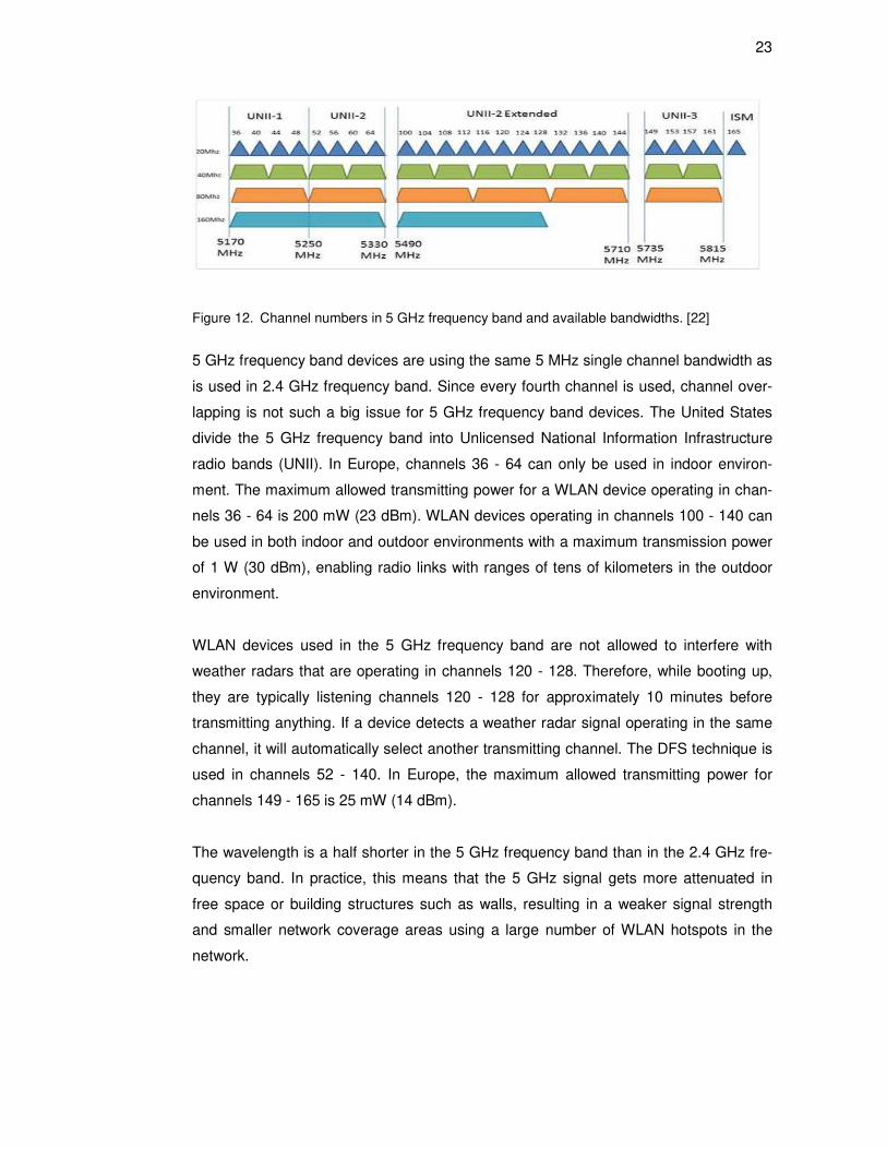
nel numbers and available bandwidths for 5 GHz frequency band are shown in figure
12.
23
Figure 12. Channel numbers in 5 GHz frequency band and available bandwidths. [22]
5 GHz frequency band devices are using the same 5 MHz single channel bandwidth as
is used in 2.4 GHz frequency band. Since every fourth channel is used, channel over-
lapping is not such a big issue for 5 GHz frequency band devices. The United States
divide the 5 GHz frequency band into Unlicensed National Information Infrastructure
radio bands (UNII). In Europe, channels 36 - 64 can only be used in indoor environ-
ment. The maximum allowed transmitting power for a WLAN device operating in chan-
nels 36 - 64 is 200 mW (23 dBm). WLAN devices operating in channels 100 - 140 can
be used in both indoor and outdoor environments with a maximum transmission power
of 1 W (30 dBm), enabling radio links with ranges of tens of kilometers in the outdoor
environment.
WLAN devices used in the 5 GHz frequency band are not allowed to interfere with
weather radars that are operating in channels 120 - 128. Therefore, while booting up,
they are typically listening channels 120 - 128 for approximately 10 minutes before
transmitting anything. If a device detects a weather radar signal operating in the same
channel, it will automatically select another transmitting channel. The DFS technique is
used in channels 52 - 140. In Europe, the maximum allowed transmitting power for
channels 149 - 165 is 25 mW (14 dBm).
The wavelength is a half shorter in the 5 GHz frequency band than in the 2.4 GHz fre-
quency band. In practice, this means that the 5 GHz signal gets more attenuated in
free space or building structures such as walls, resulting in a weaker signal strength
and smaller network coverage areas using a large number of WLAN hotspots in the
network.

24
3.5 Basic operating principles of measurement devices
3.5.1 Measurement antennas
This chapter provides an overview for general antenna characteristics that need to be
considered when choosing an antenna for RF-interference signal measurements. A
comprehensive antenna theory describing complex mathematical expressions and for-
mulas is not part of the overall scope of this study.
An antenna basically converts conducted waves into electromagnetic waves, which are
then propagating freely in space. An antenna is a reciprocal device, meaning that char-
acteristics and parameters used to describe its functionality are equally valid for trans-
mitting and receiving antennas. [23; p.9]
The most important antenna characteristics typically used for selecting an appropriate
antenna for measurement applications are listed below. [23; p.2]
• Polarization
• Radiation density
• Radiation pattern
• Directivity
• Gain
• Effective area
• Input and nominal Impedance
• Impedance matching and VSWR
• Antenna factor
• Bandwidth of an antenna
The plane electromagnetic wave can be characterized by electric and magnetic fields
traveling in one direction. Electric and magnetic fields are perpendicular to each other
and to the direction the plane wave is propagating. Antenna polarization is determined
by the direction of radiated electric field (E), evaluated in a far field. Polarization can
further be classified as linear polarization, circular polarization and elliptical polariza-
tion. Figure 13 illustrates the plane electromagnetic wave traveling in one direction and
the magnitude and direction of its E field vector in case of linear vertical polarization
and right hand circular polarization. [23; p.8]
25
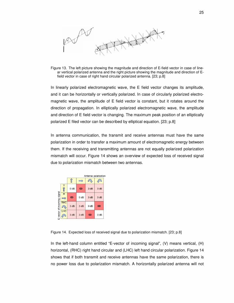
Figure 13. The left picture showing the magnitude and direction of E-field vector in case of line-ar vertical polarized antenna and the right picture showing the magnitude and direction of E-field vector in case of right hand circular polarized antenna. [23; p.8]
In linearly polarized electromagnetic wave, the E field vector changes its amplitude,
and it can be horizontally or vertically polarized. In case of circularly polarized electro-
magnetic wave, the amplitude of E field vector is constant, but it rotates around the
direction of propagation. In elliptically polarized electromagnetic wave, the amplitude
and direction of E field vector is changing. The maximum peak position of an elliptically
polarized E filed vector can be described by elliptical equation. [23; p.8]
In antenna communication, the transmit and receive antennas must have the same
polarization in order to transfer a maximum amount of electromagnetic energy between
them. If the receiving and transmitting antennas are not equally polarized polarization
mismatch will occur. Figure 14 shows an overview of expected loss of received signal
due to polarization mismatch between two antennas.
Figure 14. Expected loss of received signal due to polarization mismatch. [23; p.8]
In the left-hand column entitled “E-vector of incoming signal”, (V) means vertical, (H)
horizontal, (RHC) right hand circular and (LHC) left hand circular polarization. Figure 14
shows that if both transmit and receive antennas have the same polarization, there is
no power loss due to polarization mismatch. A horizontally polarized antenna will not
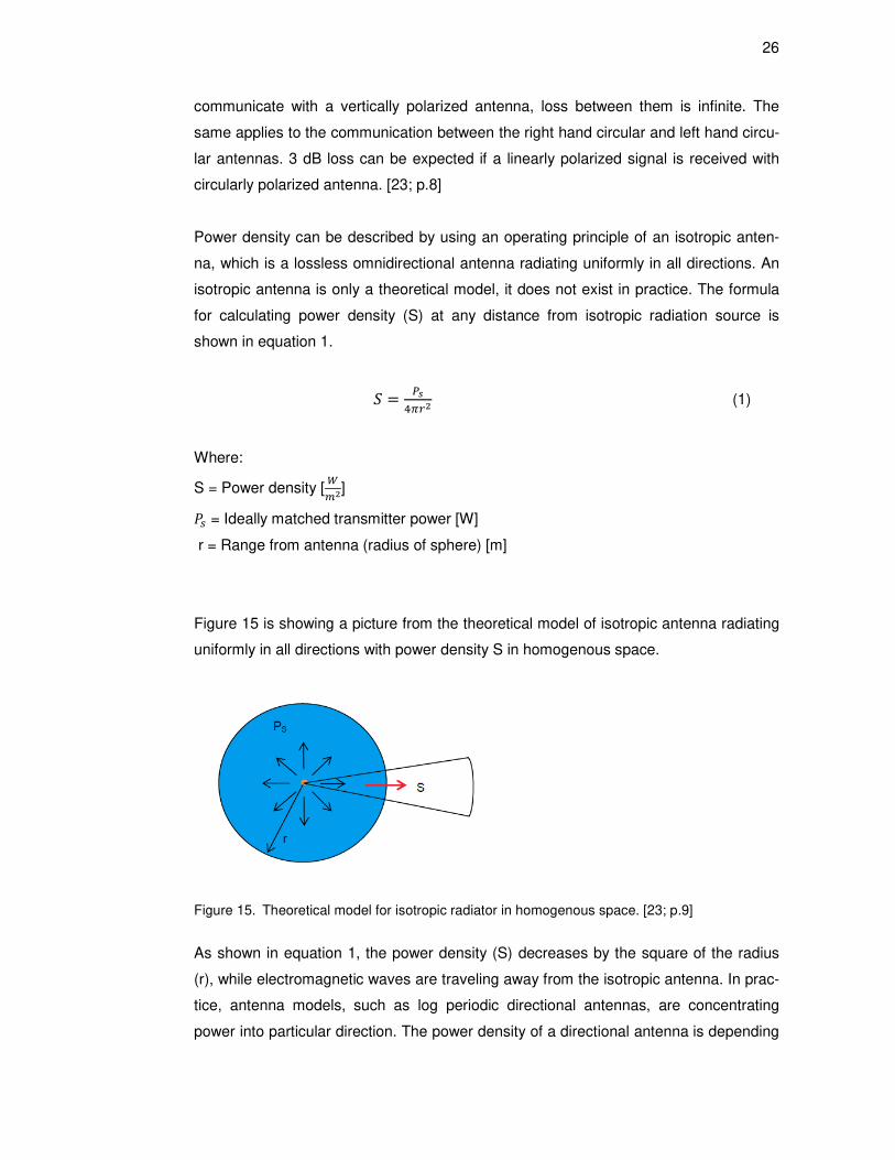
26
communicate with a vertically polarized antenna, loss between them is infinite. The
same applies to the communication between the right hand circular and left hand circu-
lar antennas. 3 dB loss can be expected if a linearly polarized signal is received with
circularly polarized antenna. [23; p.8]
Power density can be described by using an operating principle of an isotropic anten-
na, which is a lossless omnidirectional antenna radiating uniformly in all directions. An
isotropic antenna is only a theoretical model, it does not exist in practice. The formula
for calculating power density (S) at any distance from isotropic radiation source is
shown in equation 1.
= (1)
Where:
S = Power density [
]
= Ideally matched transmitter power [W]
r = Range from antenna (radius of sphere) [m]
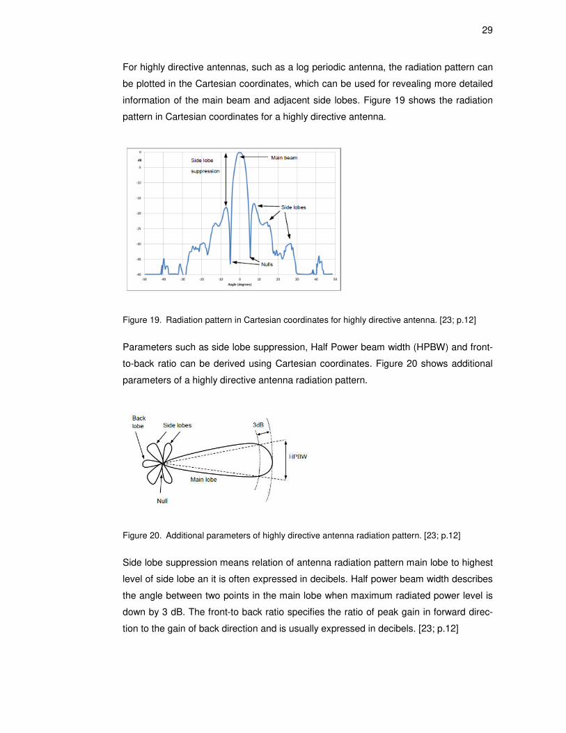
Figure 15 is showing a picture from the theoretical model of isotropic antenna radiating
uniformly in all directions with power density S in homogenous space.
Figure 15. Theoretical model for isotropic radiator in homogenous space. [23; p.9]
As shown in equation 1, the power density (S) decreases by the square of the radius
(r), while electromagnetic waves are traveling away from the isotropic antenna. In prac-
tice, antenna models, such as log periodic directional antennas, are concentrating
power into particular direction. The power density of a directional antenna is depending

27
on the practical gain of an antenna in addition to transmitted power, surface area of a
sphere and the distance from an antenna. [23; p.9]
Radiation pattern describes the three-dimensional radiation behavior of an antenna
observed in the antenna’s far field. It is a visualized presentation showing the variation
of the transmitted power radiated by an antenna as a function of direction pointing
away from an antenna. Antennas, such as dipoles and monopoles, possess directivity,
as shown in figure 16. [23; p.10]
Figure 16. Three dimension radiation pattern of dipole antenna. [23; p.10]
Dipole has a donut shape or toroidal radiation pattern. Figure 16 shows that very little
power is transmitted in the direction of antenna’s z-axis, showing nulls in the radiation
pattern. The maximum of radiation pattern for the dipole antenna is concentrated in the
directions of the x- and y-axis.
In reality, all antenna radiation patterns are three-dimensional. Radiation behavior of an
antenna can be described with horizontal and vertical patterns, which are visualized in
polar coordinates. The radiation behavior of an antenna can be characterized by using
these two patterns with well-known antenna types and patterns. A dipole antenna can
be mounted both horizontally and vertically. The horizontal radiation pattern for a verti-
cally mounted dipole antenna is shown in figure 17. [23; p.11]

28
Figure 17. Horizontal radiation pattern of vertically mounted dipole antenna. [23; p.11]
A vertically mounted dipole antenna is radiating equally in all directions in the horizontal
plane as shown in figure 17. The vertical radiation pattern of a vertically mounted dipole
antenna is shown in figure 18.
Figure 18. Vertical radiation pattern of vertically mounted dipole antenna. [23; p.11]
Figure 18 shows that a vertically mounted dipole is not radiating equally in all directions
in the vertical plane. Nulls of the radiation pattern can be seen in the directions of 0 and
180 degrees. Vertical radiation patterns for the dipole antenna are no longer circular,
they are flattened.
29
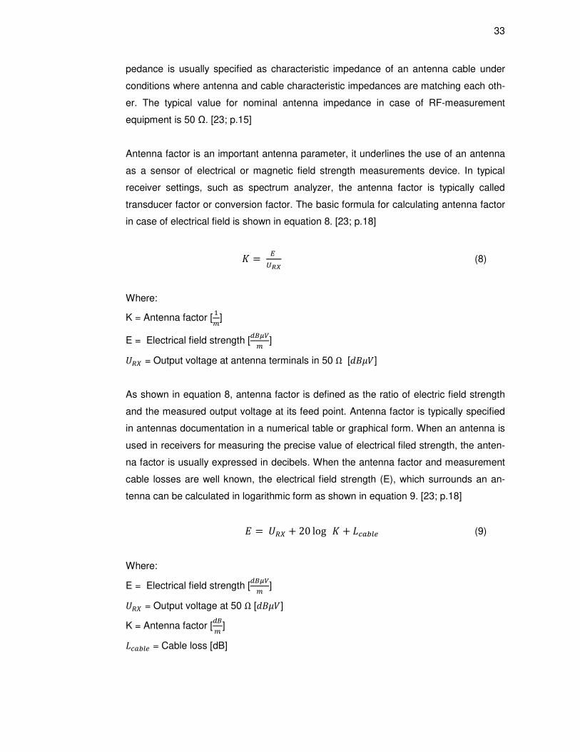
For highly directive antennas, such as a log periodic antenna, the radiation pattern can
be plotted in the Cartesian coordinates, which can be used for revealing more detailed
information of the main beam and adjacent side lobes. Figure 19 shows the radiation
pattern in Cartesian coordinates for a highly directive antenna.
Figure 19. Radiation pattern in Cartesian coordinates for highly directive antenna. [23; p.12]
Parameters such as side lobe suppression, Half Power beam width (HPBW) and front-
to-back ratio can be derived using Cartesian coordinates. Figure 20 shows additional
parameters of a highly directive antenna radiation pattern.
Figure 20. Additional parameters of highly directive antenna radiation pattern. [23; p.12]
Side lobe suppression means relation of antenna radiation pattern main lobe to highest
level of side lobe an it is often expressed in decibels. Half power beam width describes
the angle between two points in the main lobe when maximum radiated power level is
down by 3 dB. The front-to back ratio specifies the ratio of peak gain in forward direc-
tion to the gain of back direction and is usually expressed in decibels. [23; p.12]

30
Directivity is an important parameter of an antenna. It is used for describing how direc-
tional antenna radiation pattern is. An isotropic antenna radiates equally in all direc-
tions. It has zero directionality, thus its directivity factor expressed in linear form is 1 or
0 dB in logarithmic form. An increased directivity means more focused antenna radia-
tion pattern. The basic formula for calculating antenna directivity (D) is shown in equa-
tion 2. [23; p.13]
=
(2)
Where:
D = Directivity
= Radiation intensity achieved in the main direction of radiation
= = Radiation intensity for loss-free isotropic radiator with the same radiated
power
Directivity (D) can be expressed as a ratio of transmitted radiation intensity ac-
quired in the main radiation direction to radiation intensity , transmitted by isotropic
antenna with the same amount of radiated power . [23; p.13]
Antennas used in devices such as car radio, cell phones or WiFi hotspots are transmit-
ting and receiving power from all directions, therefore they have low directivity factor. In
application areas, such as satellite communication, dish antennas are often used, be-
cause transmitted or received power has to be precisely focused into the certain direc-
tion. This means in practice that dish antennas have a high directivity factor.
An antenna gain is describing how much an antenna is transmitting power in the main
direction of radiation compared to an omnidirectional isotropic antenna source with the
same input power. An antenna gain is corresponding to directivity. The formula for cal-
culating antenna gain (G) is show in equation 3. [23; p.13]

31
= ∗ (3)
Where:
G = Antenna gain
= Antenna efficiency factor
D = Directivity
Antenna efficiency factor 100% means that antenna gain and directivity would be
equal. However, in most of the practical antennas this is possible. Therefore gain can
be more easily determined with practical measurements, thus it is more often used for
characterizing an antenna. [23; p.13]. Antenna gain is often expressed in logarithmic
form as shown in equation 4.
= 10 log (4)
Where:
g = Antenna gain [dB]
G = Antenna gain
When presenting antenna gain in logarithmic form, the reference is indicated with an
additional letter after dB. Antenna gain, which is referred to isotropic radiator is indicat-
ed in units of dBi and antenna gain, which is referred to half wave dipole is indicated in
units of dBd, where 0 dBd is approximately 2.15 dBi. [23; p.13].
For example, antenna gain of 3 dBi means that the power received or transmitted from
the antenna input terminal will be two times higher compared to lossless isotropic an-
tenna with the same input power.
Effective area of an antenna is a parameter, which is normally used for characterizing
receiving antennas. Effective area describes how much power a receiving antenna is
capturing from the plane wave that is transmitted towards the receiving antenna. The
basic formula for calculating the antenna effective area (#$) is shown in equation 5.
= ∗ #$ (5)

32
Where:
#$ = Effective area [%&]
= Maximum received power [w]
S = Power density [
]
Effective area is representing how much the receiving antenna is capturing power from
the plane wave that is delivered to antenna input terminals. In real antennas, the effec-
tive area of an antenna can be calculated by means of measured antenna gain and
known wavelength as shown in equation 6.
#$ = '
(6)
Where:
#$ = Effective area [%&]
G = Antenna gain
( = Wavelength [m]
An input impedance is an important antenna parameter and it is relating to voltages
and currents at the input terminal of an antenna. The basic formula for calculating input
impedance ()*) of an antenna is shown in equation 7. [23; p.14]
)* = (,- + ,/) + 12* (7)
Where:
)* = Input impedance at input terminal of an antenna [Ω]
,- = Radiation resistance [Ω]
,/ = Loss resistance [Ω]
12* = Imaginary part of input impedance at input terminal of an antenna [Ω]
Real part of input impedance present at the antenna feed point is split into the radiation
resistance and ,- and loss resistance ,/. [23; p. 14]. Imaginary part of an antenna
input impedance consists of capacitive and inductive impedance values. For electrically
short linear antennas, the imaginary part of input impedance is capacitive, and in case
of electrically long linear antennas it is inductive. The imaginary part of an antenna im-
pedance is zero, when the antenna is operating at resonance. Nominal antenna im-
33
pedance is usually specified as characteristic impedance of an antenna cable under
conditions where antenna and cable characteristic impedances are matching each oth-
er. The typical value for nominal antenna impedance in case of RF-measurement
equipment is 50 Ω. [23; p.15]
Antenna factor is an important antenna parameter, it underlines the use of an antenna
as a sensor of electrical or magnetic field strength measurements device. In typical
receiver settings, such as spectrum analyzer, the antenna factor is typically called
transducer factor or conversion factor. The basic formula for calculating antenna factor
in case of electrical field is shown in equation 8. [23; p.18]
3 = 4 567
(8)
Where:
K = Antenna factor [8]
E = Electrical field strength [9:;<
]
=-> = Output voltage at antenna terminals in 50 Ω [@ABC]
As shown in equation 8, antenna factor is defined as the ratio of electric field strength
and the measured output voltage at its feed point. Antenna factor is typically specified
in antennas documentation in a numerical table or graphical form. When an antenna is
used in receivers for measuring the precise value of electrical filed strength, the anten-
na factor is usually expressed in decibels. When the antenna factor and measurement
cable losses are well known, the electrical field strength (E), which surrounds an an-
tenna can be calculated in logarithmic form as shown in equation 9. [23; p.18]
D = =-> + 20 log 3 + FGHIJ (9)
Where:
E = Electrical field strength [9:;<
]
=-> = Output voltage at 50 Ω [@ABC]
K = Antenna factor [9: ]
FGHIJ = Cable loss [dB]
34
Important terms in antenna design and engineering are gain and directivity. In case
antenna factor data is not specified in the datasheet, it is possible to calculate the an-
tenna factor when antenna gain and measurement frequency are known. The conver-
sion between antenna gain and antenna factor in decibels is shown in equation 10. [23;
p.18]
K = −29.8 @A + 20 log P QRSTU − (10)
Where:
k = Antenna factor [dB]
f = Measured frequency [MHz]
g = Antenna gain [dB]
The bandwidth of an antenna describes the range of usable frequencies over which an
antenna can properly radiate or receive energy. It is common practice to use an im-
pedance match VSWR < 1.5 value for determining the antenna bandwidth. The basic
formula for calculating the bandwidth for broadband antennas is shown in equation 11.
AV = WX
(11)
Where:
BW = Bandwidth of an antenna [Hz]
S = Highest usable frequency [Hz]
/ = Lowest usable frequency [Hz]
An antenna can be characterized to be broadband when the calculated result in equa-
tion 11 is greater than 2. A formula for calculating the antenna bandwidth for narrow-
band antenna is shown in equation 12. [23; p.19]
AV = PQWY QXQZ
U ∗ 100 (12)
35
Where:
BW = Bandwidth of an antenna [%]
[S = Highest usable frequency [Hz]
[/ = Lowest usable frequency [Hz]
[\ = Center frequency [Hz]
Values in equation 12 can range between 0% and 200% but are in practice only used
up to 100%.
3.5.2 Spectrum analyzer
This chapter provides a basic overview of the operating principle for swept tuned and
modern FFT (Fast Fourier Transform) based spectrum analyzer technologies and their
main performance features. A complete description and detailed operating principle of
a spectrum analyzer is not part for the scope of this this study. The main setting pa-
rameters and performance features needed for interference hunting in the WLAN net-
work are included in this chapter.
Spectrum analyzer is measuring the amplitude of an input signals frequency compo-
nent within the limits of full frequency range of the instrument. The primary use for the
spectrum analyzer is to measure the power level of spectrum for both known and un-
known RF signals. The measured signal is displayed on the screen, where the x-axis
presents the frequency of measured spectrum and the y-axis the amplitude of the
spectrum. Measurement results are usually presented in logarithmic scale for both axis.
Spectrum analyzer technology has evolved a lot since 1960s when the first models
came into the markets. Traditional spectrum analyzers are swept-tuned instruments
using the operating principal of super heterodyne receiver. There are three basic types
of spectrum analyzers in the market: swept-tuned spectrum analyzer, FFT-based spec-
trum analyzer and real-time FFT-based spectrum analyzer. Most of the modern day
spectrum analyzers are based on FFT technology, but a high number of swept-tuned
spectrum analyzers are still in use. A simplified block diagram of a conventional swept-
tuned spectrum analyzer operating on the heterodyne principle is shown in figure 21.

36
Figure 21. Simplified block diagram of swept tuned spectrum analyzer based on heterodyne receiver design. [24; p.28]
The heterodyne receiver inside the spectrum analyzer is converting the input signal into
intermediate frequency (IF) with the aid of a local oscillator (LO) and a mixer. Complete
input frequency range of analyzer can be converted into a constant intermediate fre-
quency with the aid of tunable local oscillator. A converted IF signal is fed through the
IF amplifier stage before it is fed to the IF filter stage. The resolution bandwidth (RBW)
of the spectrum analyzer is determined by fix-tuned IF filters at the intermediate fre-
quency stage. [24; p.28]
Logarithmic amplifier is used for allowing signals in a wide level of range to be dis-
played on the screen by compressing the IF signal. The envelope of the IF signal is
detected by an envelope detector resulting into a video signal. This signal is averaged
with the aid of an adjustable low pass video filter stage. The averaged noise free and
smoothed signal is fed into the vertical deflection of display unit. Sawtooth signal is
used for driving horizontal deflection of display unit and local oscillator stage, because
the received signal is displayed as a function of frequency. [24; p.29]
In a modern swept tuned spectrum analyzer, all processes are controlled by several
microprocessors. The input signal is sampled in signal chain by the aid of an ADC con-
verter using fast digital signal processors. In the older instruments, the video signal was
sampled after an analog envelope detector and video filter stage. In the modern spec-
trum analyzer, the video signal is digitized to low intermediate frequency and the enve-
lope of the IF signal is determined from digitized samples. In modern analyzers, the
local oscillator is no longer tuned with the aid of a sawtooth signal; instead, it is locked

37
to reference frequency via a phase locked loop (PLL). Frequency tuning is done by
varying division factors inside the PLL, resulting to a higher frequency accuracy. In the
modern spectrum analyzer, cathode ray tubes are replaced by a liquid crystal display
(LCD), allowing the use of a more compact design. [24; p.30]
Most of the modern day spectrum analyzers are based on FFT technology. The fre-
quency spectrum of the measured signal is defined by the signal time characteristics.
The time and frequency domain can be linked to each other by means of Fourier trans-
form. The frequency resolution of the FFT based spectrum analyzer can be determined
by calculating the inverse of time over which the waveform is measured and Fourier
transformed. In practical FFT based analyzers, the Fourier transform is made with the
aid of powerful signal processing. Simplified block diagram from the FFT based spec-
trum analyzer is shown in figure 22. [24; p.18]
Figure 22. Simplified block diagram of FFT based spectrum analyzer design. [24; p.25]
The bandwidth of an input signal is limited by the analog low pass filter in order to ad-
here to the sampling theorem. As a general rule the sampling frequency of an ADC
converter has to be at least twice the bandwidth of the input signal. The Fourier trans-
form will then produce a spectrum containing all frequencies, without aliasing effects.
After the signal has been sampled, the quantized values are stored in random access
memory (RAM). The stored values are calculated in frequency domain by the aid of
the FFT processor and finally displayed in LCD screen. [24; p.25]
The ADC converter is producing quantization noise due to the quantization of samples.
This will cause a limitation to the dynamic range of the analyzer. The higher the num-
ber of bits used in the ADC converter is, the lower the quantization noise. In practice,
high resolution ADC converters have a limited available bandwidth, therefore a com-
promise between the analyzer dynamic range and the input frequency range has to be
found. [24; p.26]

38
Pure FFT based spectrum analyzers are capable of measuring narrow band signals
while maintaining a good dynamic range. One technique to expand the input frequency
range and to maintain a good dynamic range is to combine the superheterodyne and
FFT analyzer together into a so-called hybrid superheterodyne FFT analyzer. In this
method, the input signal is first down-converted into intermediated frequency and then
digitized. Superheterodyne or FFT techniques are then used to acquire the spectrum. A
hybrid superheterodyne FFT analyzer allows faster sweep times to be used during the
measurements. Another benefit is usage of digital RBW filters, with a near perfect
shape factor and improved settling time, which cannot be achieved with conventional
analog filters. [24; p.26]
Both swept-tuned and hybrid superheterodyne analyzers have a so-called blind time
due to frequency sweep, a sampling time of the ADC converter and an FFT processing
and calculation time. During the blind time period, information from measured spectrum
could be missed. A real time FFT spectrum analyzer is able to sample the input RF
signal in the time domain and convert the information back to the frequency domain
using the FFT processing without a blind time period. Typically parallel, gapless and
overlapped FFT processing is applied in order to acquire an RF spectrum that is not
missing any information. The typical real time bandwidth in the modern spectrum ana-
lyzers is 800 MHz or even more.
Basic settings that have to be set by the user for spectrum analyzer in order to meas-
ure RF signals, such as continuous wave (CW), are listed below:
• Range of displayed frequencies
• Range of displayed signal levels
• Resolution bandwidth
• Sweep time.
The frequency display range can be set by the start and stop frequency range or by the
exact center frequency and span around the center frequency. The level display range
is used for setting the reference level for maximum signal level to be displayed. Fre-
quency resolution of the spectrum analyzer is set via resolution bandwidth at the IF
filter stage. The time which is required to sweep and record the entire selected fre-
quency span is called sweep time. An example of the measured CW signal spectrum is
shown in figure 23. [24; p.31]
39
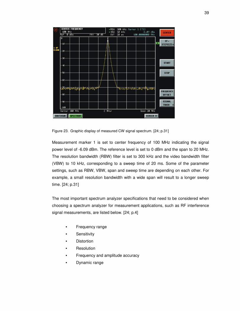
Figure 23. Graphic display of measured CW signal spectrum. [24; p.31]
Measurement marker 1 is set to center frequency of 100 MHz indicating the signal
power level of -6.09 dBm. The reference level is set to 0 dBm and the span to 20 MHz.
The resolution bandwidth (RBW) filter is set to 300 kHz and the video bandwidth filter
(VBW) to 10 kHz, corresponding to a sweep time of 20 ms. Some of the parameter
settings, such as RBW, VBW, span and sweep time are depending on each other. For
example, a small resolution bandwidth with a wide span will result to a longer sweep
time. [24; p.31]
The most important spectrum analyzer specifications that need to be considered when
choosing a spectrum analyzer for measurement applications, such as RF interference
signal measurements, are listed below. [24; p.4]
• Frequency range
• Sensitivity
• Distortion
• Resolution
• Frequency and amplitude accuracy
• Dynamic range
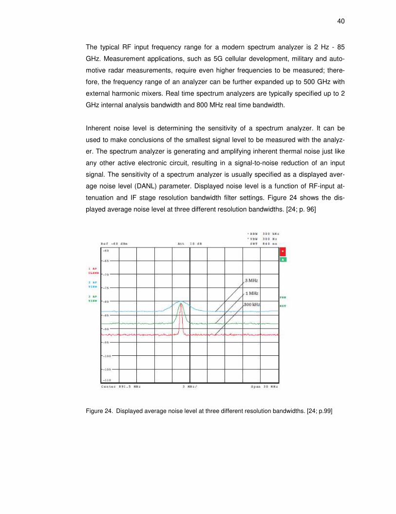
40
The typical RF input frequency range for a modern spectrum analyzer is 2 Hz - 85
GHz. Measurement applications, such as 5G cellular development, military and auto-
motive radar measurements, require even higher frequencies to be measured; there-
fore, the frequency range of an analyzer can be further expanded up to 500 GHz with
external harmonic mixers. Real time spectrum analyzers are typically specified up to 2
GHz internal analysis bandwidth and 800 MHz real time bandwidth.
Inherent noise level is determining the sensitivity of a spectrum analyzer. It can be
used to make conclusions of the smallest signal level to be measured with the analyz-
er. The spectrum analyzer is generating and amplifying inherent thermal noise just like
any other active electronic circuit, resulting in a signal-to-noise reduction of an input
signal. The sensitivity of a spectrum analyzer is usually specified as a displayed aver-
age noise level (DANL) parameter. Displayed noise level is a function of RF-input at-
tenuation and IF stage resolution bandwidth filter settings. Figure 24 shows the dis-
played average noise level at three different resolution bandwidths. [24; p. 96]
Figure 24. Displayed average noise level at three different resolution bandwidths. [24; p.99]

41
The maximum sensitivity of a spectrum analyzer is achieved when the RF input attenu-
ation of 0 dB and narrowest available resolution bandwidth is used. Figure 24 shows
the average noise level measured with three different resolution bandwidth settings
using 10 dB RF input attenuation. The average noise level of an analyzer is decreased
when the resolution bandwidth is decreased, as can be seen from the blue, green and
red traces. As a general rule, the signal-to-noise ratio of a spectrum analyzer is de-
creased when the RF input attenuation is increased, therefore affecting the sensitivity
of an analyzer. The sensitivity of an analyzer can be enhanced with the aid of a pre-
amplifier. A low displayed average noise level leads to a better sensitivity and perfor-
mance of the spectrum analyzer, allowing measurements for low power signal levels.
[24; p.101]
Spectrum analyzers are typically used in measurement applications for amplifiers and
mixers, which are producing distortion in form of harmonics and intermodulation prod-
ucts. First mixer inside the spectrum analyzer is generating harmonic and intermodula-
tion distortion especially with high level of input signals, which is then added to those
produced in the measured device. For single tone input signals, such as the sinusoidal
signal, the specifications in the spectrum analyzer datasheets are usually referring to
the level of second harmonic signal. This parameter is usually specified as second
harmonic intercept (SHI) point in the datasheets. [24; p.103]
In addition to harmonics, signals consisting of two tones are producing intermodulation
signal distortion, which are even and odd numbered. Even numbered distortion prod-
ucts always occur far away from two original input signal frequencies. Low order odd
numbered intermodulation products are created in close vicinity of the original input
signals, therefore they are difficult to filter away. Usually second and third order inter-
cept points are specified in analyzer datasheets for nonlinearities, such as intermodula-
tion distortion products created by the spectrum analyzer inside the first mixer. An ex-
ample of the second and third order intercept point specification is presented in figure
25. [24; p.104]
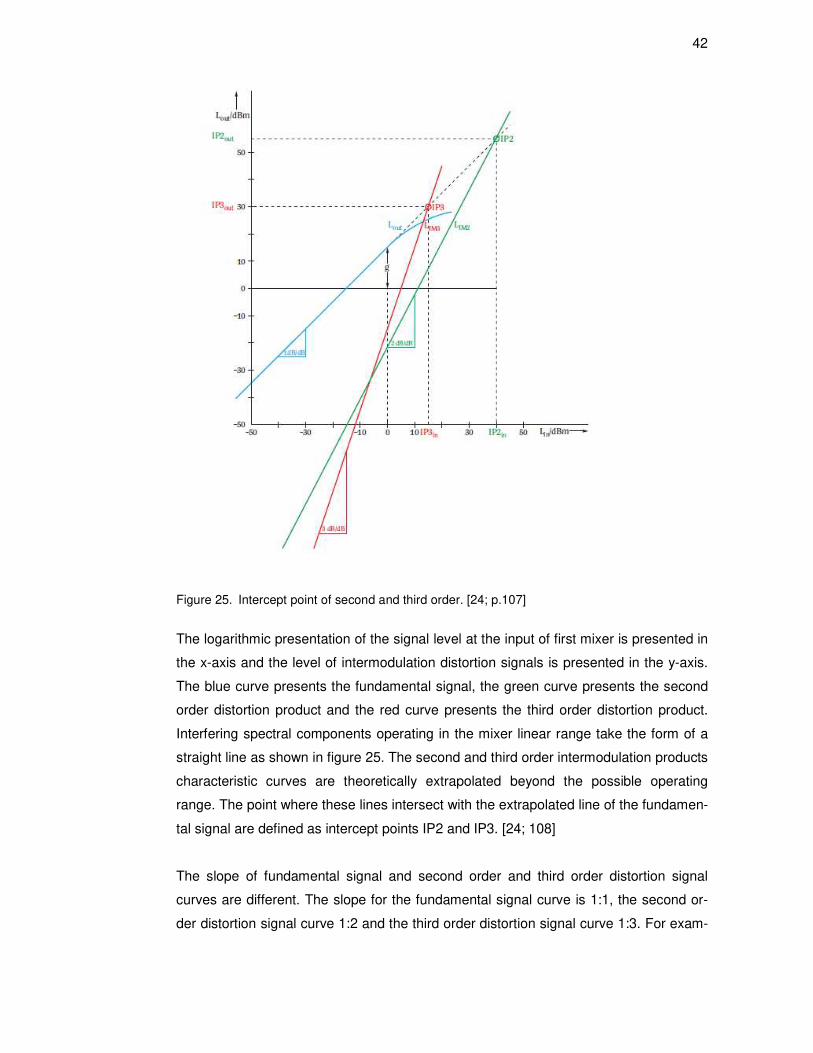
42
Figure 25. Intercept point of second and third order. [24; p.107]
The logarithmic presentation of the signal level at the input of first mixer is presented in
the x-axis and the level of intermodulation distortion signals is presented in the y-axis.
The blue curve presents the fundamental signal, the green curve presents the second
order distortion product and the red curve presents the third order distortion product.
Interfering spectral components operating in the mixer linear range take the form of a
straight line as shown in figure 25. The second and third order intermodulation products
characteristic curves are theoretically extrapolated beyond the possible operating
range. The point where these lines intersect with the extrapolated line of the fundamen-
tal signal are defined as intercept points IP2 and IP3. [24; 108]
The slope of fundamental signal and second order and third order distortion signal
curves are different. The slope for the fundamental signal curve is 1:1, the second or-
der distortion signal curve 1:2 and the third order distortion signal curve 1:3. For exam-

43
ple, the red curve presenting the third order distortion shows that a 1 dB increase of the
fundamental signal level at the input of first mixer is causing a 3 dB increase of the dis-
tortion signal level. The blue and green curves can be interpreted respectively accord-
ing to the steepness of their slope. [24; p.108]
The linearity of the spectrum analyzer is determined by the first mixer and IF amplifier.
Harmonic and intermodulation distortion products generated by the spectrum analyzer
inside these stages can lead to incorrect measurement results. Therefore, it is very
important to maintain a proper signal level at the input of the first mixer while doing
measurements. The input level of the first mixer is adjusted automatically in most of the
modern spectrum analyzers. If the user is overriding the automatic settings and the
mixer is overdriven, a warning indication is shown at the screen of the instrument in
order to avoid incorrect measurement results. [24; p.112]
The resolution of the spectrum analyzer is determined by the type and shape factor of
the resolution bandwidth filter, selected resolution bandwidth and phase noise generat-
ed inside the analyzer’s internal oscillator circuitry. Modern analyzers are using analog,
digital and FFT based resolution bandwidth filters. Analog filters can be used for realiz-
ing large resolution bandwidths, typically 100 kHz - 10 MHz. The typical shape factor
for analog filters is about 10 - 14. Analog filters cannot be used for implementing ideal
Gaussian type filters with a good shape factor. [24; p.54]
Digital filters can be used for implementing narrow resolution bandwidths and realizing
ideal Gaussian filters with the typical shape factor of 4.6. Digital filters allow shorter
sweep times to be used than analog filters of the same bandwidth. Very narrow resolu-
tion bandwidth setting leads to a long sweep time. FFT filters are implemented to
shorten a sweep time when narrow resolution bandwidths are used. Maximum fre-
quency span that can be analyzed by the FFT resolution bandwidth filters is limited by
the sampling rate of the analyzer ADC converter and size of its sample memory. The
typical shape factor for the FFT filter is 2.6. The downsize for FFT filters is that they are
not suitable for measuring pulsed signals, and therefore, modern spectrum analyzers
contain all filter types analog, digital and FFT. [24; p. 57]
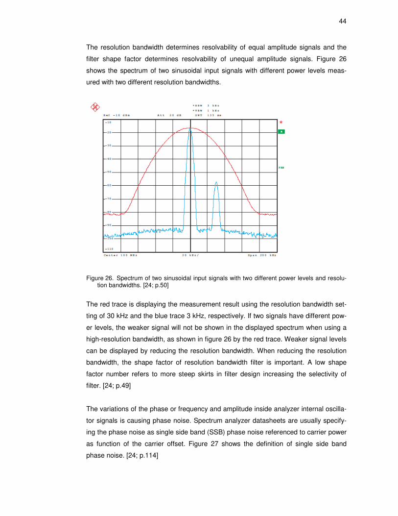
44
The resolution bandwidth determines resolvability of equal amplitude signals and the
filter shape factor determines resolvability of unequal amplitude signals. Figure 26
shows the spectrum of two sinusoidal input signals with different power levels meas-
ured with two different resolution bandwidths.
Figure 26. Spectrum of two sinusoidal input signals with two different power levels and resolu-tion bandwidths. [24; p.50]
The red trace is displaying the measurement result using the resolution bandwidth set-
ting of 30 kHz and the blue trace 3 kHz, respectively. If two signals have different pow-
er levels, the weaker signal will not be shown in the displayed spectrum when using a
high-resolution bandwidth, as shown in figure 26 by the red trace. Weaker signal levels
can be displayed by reducing the resolution bandwidth. When reducing the resolution
bandwidth, the shape factor of resolution bandwidth filter is important. A low shape
factor number refers to more steep skirts in filter design increasing the selectivity of
filter. [24; p.49]
The variations of the phase or frequency and amplitude inside analyzer internal oscilla-
tor signals is causing phase noise. Spectrum analyzer datasheets are usually specify-
ing the phase noise as single side band (SSB) phase noise referenced to carrier power
as function of the carrier offset. Figure 27 shows the definition of single side band
phase noise. [24; p.114]
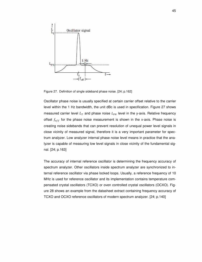
45
Figure 27. Definition of single sideband phase noise. [24; p.162]
Oscillator phase noise is usually specified at certain carrier offset relative to the carrier
level within the 1 Hz bandwidth, the unit dBc is used in specification. Figure 27 shows
measured carrier level F] and phase noise F^ level in the y-axis. Relative frequency
offset [_QQ for the phase noise measurement is shown in the x-axis. Phase noise is
creating noise sidebands that can prevent resolution of unequal power level signals in
close vicinity of measured signal, therefore it is a very important parameter for spec-
trum analyzer. Low analyzer internal phase noise level means in practice that the ana-
lyzer is capable of measuring low level signals in close vicinity of the fundamental sig-
nal. [24; p.163]
The accuracy of internal reference oscillator is determining the frequency accuracy of
spectrum analyzer. Other oscillators inside spectrum analyzer are synchronized to in-
ternal reference oscillator via phase locked loops. Usually, a reference frequency of 10
MHz is used for reference oscillator and its implementation contains temperature com-
pensated crystal oscillators (TCXO) or oven controlled crystal oscillators (OCXO). Fig-
ure 28 shows an example from the datasheet extract containing frequency accuracy of
TCXO and OCXO reference oscillators of modern spectrum analyzer. [24; p.140]

46
Figure 28. Frequency accuracy of TCXO and OCXO reference oscillators of modern spectrum analyzer. [24; p.140]
By using oven controlled crystal oscillator a very high frequency accuracy and small
temperature drift are achieved as shown in figure 28. Total frequency error depends on
temperature drift and long term frequency stability of reference oscillator. Long term
frequency stability is achieved when an analyzer remains permanently switched on.
Specifications of oscillator aging per year are typically valid after 30 days of constant
operation. [24; p.141]
The level measurement accuracy of a spectrum analyzer has always some uncertainty.
Components that contribute to uncertainty are:
• Mechanical switching uncertainty caused by RF input attenuator
• Input mismatch caused by VSWR
• Frequency response of first mixer and input filters
• Reference level accuracy of IF stage gain and attenuation
• RBW filter switching uncertainty
• Display scale fidelity caused by Log amplifier
• Amplitude accuracy of internal calibrator signal
Modern spectrum analyzers are factory calibrated before delivery. Individual measure-
ment errors for different internal stages are recorded in the factory and stored inside
the analyzer as correction values. This means in practice that the user can achieve
best level measurement accuracy by optimizing his measurement setup and tech-
niques. [24; p.141]

47
Dynamic range of spectrum analyzer means analyzer ability to simultaneously process
signals with different power levels. The limits of dynamic range is depending on the
application to be measured. Figure 29 shows an example of analyzer theoretical dy-
namic range versus real measurement range. Actual dynamic range is depending on
second and third order distortion products, 1 dB compression point, displayed average
noise level (DANL) and phase noise specification of analyzer.
Figure 29. Spectrum analyzer theoretical dynamic range versus real measurement range. [25]
As shown in figure 29, lower level of dynamic range is determined by the internal in-
herent noise level and phase noise level, generated by the analyzer in different stages.
The upper limit of dynamic range is determined by the 1 dB compression point of ana-
lyzer electronic stages or intermodulation distortion products generated inside the ana-
lyzer in case its first mixer is overdriven. [24; p.125]
The phase noise generated by analyzer local oscillator is mixed into the input signal in
the analyzer frequency converting stages such as mixers. If the measured signal level
is high, the effects of the analyzer thermal noise level can be neglected. This means in
practice that the achievable dynamic range of an analyzer at a small carrier offset is
determined solely by the local oscillator phase noise level. [24; p.167]
As shown in figure 27, the phase noise of a spectrum analyzer decreases when carrier
offset is increased. At a large carrier offset, the dynamic range of the spectrum analyz-
er is determined by the analyzer thermal noise level. This means is practice that a high
signal-to-noise ratio and 1 dB compression point is required for achieving a better dy-

48
namic range for the analyzer, when making measurements far off the carrier.
[24; p.167]
A high signal level at the input of the first mixer also create harmonics of the input sig-
nal. If these harmonics falls outside of the frequency range, which phase noise of the
device under test (DUT) is to be measured they do not cause any disturbance. In case
input signal level is greater than the analyzer dynamic range it has to be reduced by
using internal or external RF attenuator, in order to achieve reliable measurement re-
sults. [24; p.167]
4 RF-interference and data bandwidth measurements in office WLAN network
The following chapters provide a description of an experimental WLAN network test
setup, spectrum analyzer and network performance measurement procedures and test
results for RF-interference signal and data bandwidth measurements. Finally all meas-
ured RF-interference signals and recorded WLAN network data bandwidth values are
analyzed and described in more detail.
4.1 Description of test setup
The test setup used for studying physical layer characteristics of two external interferer
sources operating at 2.4 GHz ISM frequency band is described in this chapter. Physical
measurements were made in Rohde & Schwarz Finland’s sales office. Since the office
was equipped with operational public campus WLAN network, RF-interference meas-
urements were performed after normal business hours in order to avoid interfering the
campus WLAN network traffic with a microwave oven and a Bluetooth loudspeaker.
The measurement setup for experimental WLAN network was constructed inside a
storage room where operational overlapping adjacent channels from the campus
WLAN network were not interfering the measurement results and where it was possible
to achieve a suitable physical measurement arrangement.
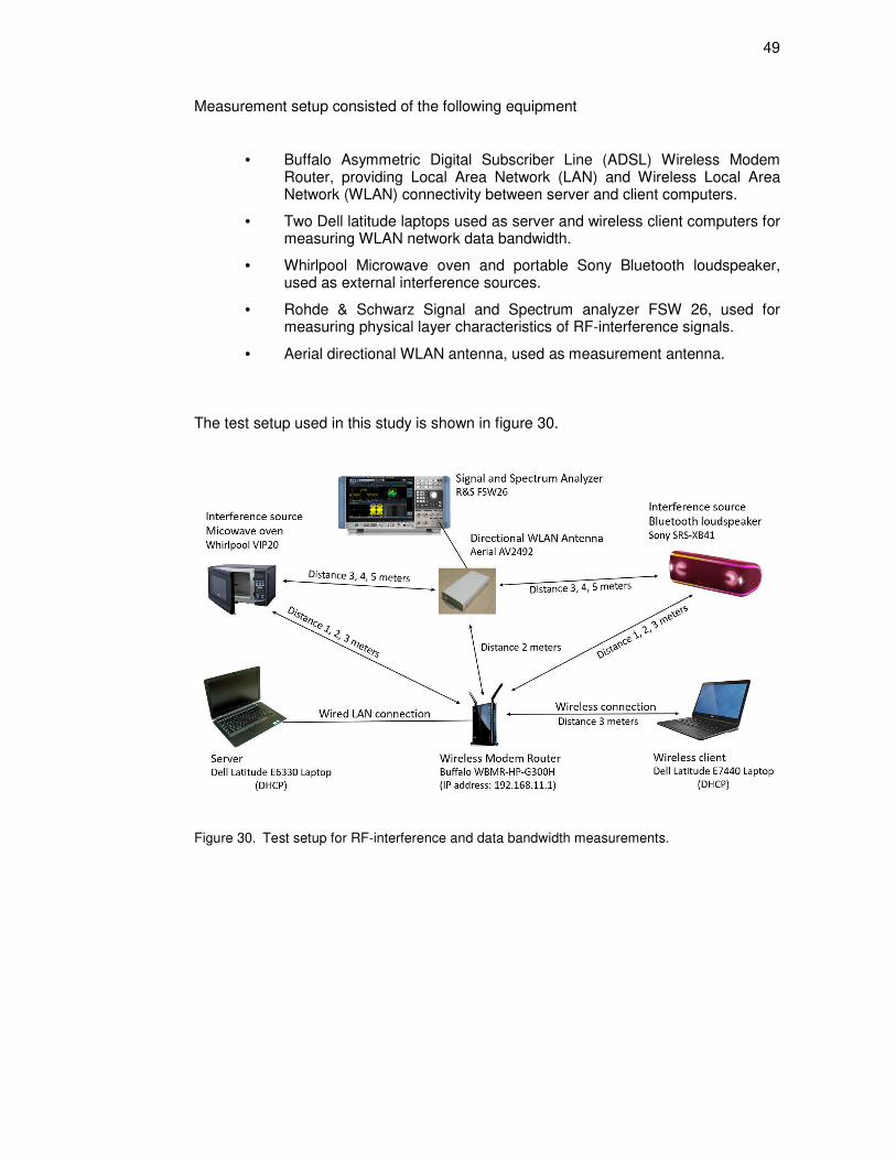
49
Measurement setup consisted of the following equipment
• Buffalo Asymmetric Digital Subscriber Line (ADSL) Wireless Modem Router, providing Local Area Network (LAN) and Wireless Local Area Network (WLAN) connectivity between server and client computers.
• Two Dell latitude laptops used as server and wireless client computers for measuring WLAN network data bandwidth.
• Whirlpool Microwave oven and portable Sony Bluetooth loudspeaker, used as external interference sources.
• Rohde & Schwarz Signal and Spectrum analyzer FSW 26, used for measuring physical layer characteristics of RF-interference signals.
• Aerial directional WLAN antenna, used as measurement antenna.
The test setup used in this study is shown in figure 30.
Figure 30. Test setup for RF-interference and data bandwidth measurements.

50
As shown in figure 30, the wireless modem router was used for providing connection
between server and client computers. The modem was not connected to the Internet
during measurements procedures. Two computers were used for measuring WLAN
network data bandwidth by utilizing a external network data bandwidth software analyz-
ing tool called jPerf [11].
A normal microwave oven and a portable Bluetooth loudspeaker were used as external
interference sources inside the experimental WLAN network. During the RF-
interference measurements a bowl of cold water was placed inside the microwave ov-
en, which was operated 180 seconds in its maximum output power of 900 W. The Blue-
tooth loudspeaker was paired with a mobile phone, streaming music from the phone.
The distance between the wireless modem router and external interference sources
were changed between 1–3 meters during different phases of measurement. Same
measurement routines were repeated three times for each external interferer sources
in order to study how physical distance affects the peak power level of interference
signal and data bandwidth of experimental WLAN network.
A directional WLAN measurement antenna was placed 2 meters away from the wire-
less modem router. The antenna was placed at a height of 1.2 meters above the floor
level by using a separate tripod. The position or the height of the antenna were not
changed during the RF-interference measurements. A modern high quality real time
spectrum analyzer was used for measuring the physical layer characteristics of RF-
interference signals coming from the microwave oven and Bluetooth loudspeaker.
The server computer was connected to the wireless modem router via category 6
twisted pair Ethernet cable in order to provide good protection against crosstalk and
external noise. A wireless connection between client computer and modem router was
established. The server and client computers were using their own built-in Network
Interface Cards (NIC) for generating network traffic for data bandwidth measurements.
In order to measure reliable data bandwidth values between server and client comput-
ers, the IP-addresses of both computers had to be configured into the same subnet-
work. Both computers were using the Dynamic Host Configuration Protocol (DHCP) in
order to automatically fetch the IP-address from the wireless modem router DHCP ad-
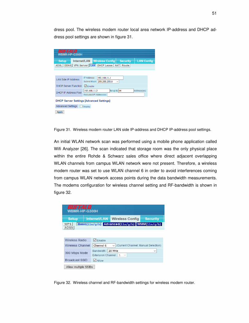
51
dress pool. The wireless modem router local area network IP-address and DHCP ad-
dress pool settings are shown in figure 31.
Figure 31. Wireless modem router LAN side IP-address and DHCP IP-address pool settings.
An initial WLAN network scan was performed using a mobile phone application called
Wifi Analyzer [26]. The scan indicated that storage room was the only physical place
within the entire Rohde & Schwarz sales office where direct adjacent overlapping
WLAN channels from campus WLAN network were not present. Therefore, a wireless
modem router was set to use WLAN channel 6 in order to avoid interferences coming
from campus WLAN network access points during the data bandwidth measurements.
The modems configuration for wireless channel setting and RF-bandwidth is shown in
figure 32.
Figure 32. Wireless channel and RF-bandwidth settings for wireless modem router.
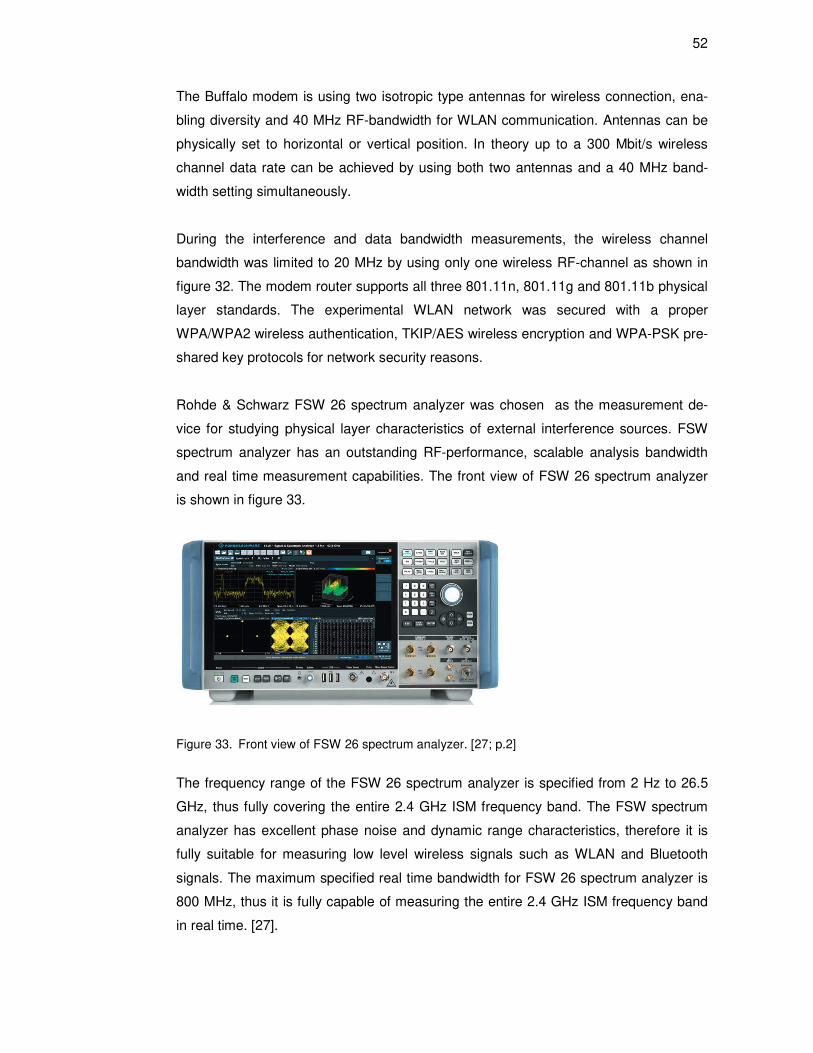
52
The Buffalo modem is using two isotropic type antennas for wireless connection, ena-
bling diversity and 40 MHz RF-bandwidth for WLAN communication. Antennas can be
physically set to horizontal or vertical position. In theory up to a 300 Mbit/s wireless
channel data rate can be achieved by using both two antennas and a 40 MHz band-
width setting simultaneously.
During the interference and data bandwidth measurements, the wireless channel
bandwidth was limited to 20 MHz by using only one wireless RF-channel as shown in
figure 32. The modem router supports all three 801.11n, 801.11g and 801.11b physical
layer standards. The experimental WLAN network was secured with a proper
WPA/WPA2 wireless authentication, TKIP/AES wireless encryption and WPA-PSK pre-
shared key protocols for network security reasons.
Rohde & Schwarz FSW 26 spectrum analyzer was chosen as the measurement de-
vice for studying physical layer characteristics of external interference sources. FSW
spectrum analyzer has an outstanding RF-performance, scalable analysis bandwidth
and real time measurement capabilities. The front view of FSW 26 spectrum analyzer
is shown in figure 33.
Figure 33. Front view of FSW 26 spectrum analyzer. [27; p.2]
The frequency range of the FSW 26 spectrum analyzer is specified from 2 Hz to 26.5
GHz, thus fully covering the entire 2.4 GHz ISM frequency band. The FSW spectrum
analyzer has excellent phase noise and dynamic range characteristics, therefore it is
fully suitable for measuring low level wireless signals such as WLAN and Bluetooth
signals. The maximum specified real time bandwidth for FSW 26 spectrum analyzer is
800 MHz, thus it is fully capable of measuring the entire 2.4 GHz ISM frequency band
in real time. [27].

53
Aerial directional WLAN measurement antenna was chosen for interference measure-
ments. Figure 34 shows a picture of the measurement antenna setup.
Figure 34. Measurement antenna setup.
The antenna setup consisted of Aerial AV2492 antenna module, antenna cable and
tripod as shown in figure 34. The frequency range of antenna module is from 2.4 GHz -
2.5 GHz, thus fully covering the entire 2.4 GHz ISM frequency band. The polarization of
an antenna is vertical, therefore it is capable of receiving a maximum amount of energy
from vertically polarized wireless modem router antennas. The nominal impedance of
AV2492 antenna is 50 ohms, it can be connected directly via a 50 ohm cable into the
input of the spectrum analyzer without using separate impedance converters. Antenna
E-plane, H-plane and gain values are specified at the factory during the manufacturing
process. The characteristics of Aerial AV2492 WLAN antenna module are shown in
table 2. [28; p.13]
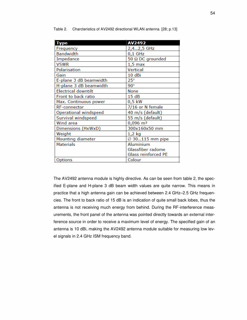
54
Table 2. Charcteristics of AV2492 directional WLAN antenna. [28; p.13]
The AV2492 antenna module is highly directive. As can be seen from table 2, the spec-
ified E-plane and H-plane 3 dB beam width values are quite narrow. This means in
practice that a high antenna gain can be achieved between 2.4 GHz–2.5 GHz frequen-
cies. The front to back ratio of 15 dB is an indication of quite small back lobes, thus the
antenna is not receiving much energy from behind. During the RF-interference meas-
urements, the front panel of the antenna was pointed directly towards an external inter-
ference source in order to receive a maximum level of energy. The specified gain of an
antenna is 10 dBi, making the AV2492 antenna module suitable for measuring low lev-
el signals in 2.4 GHz ISM frequency band.
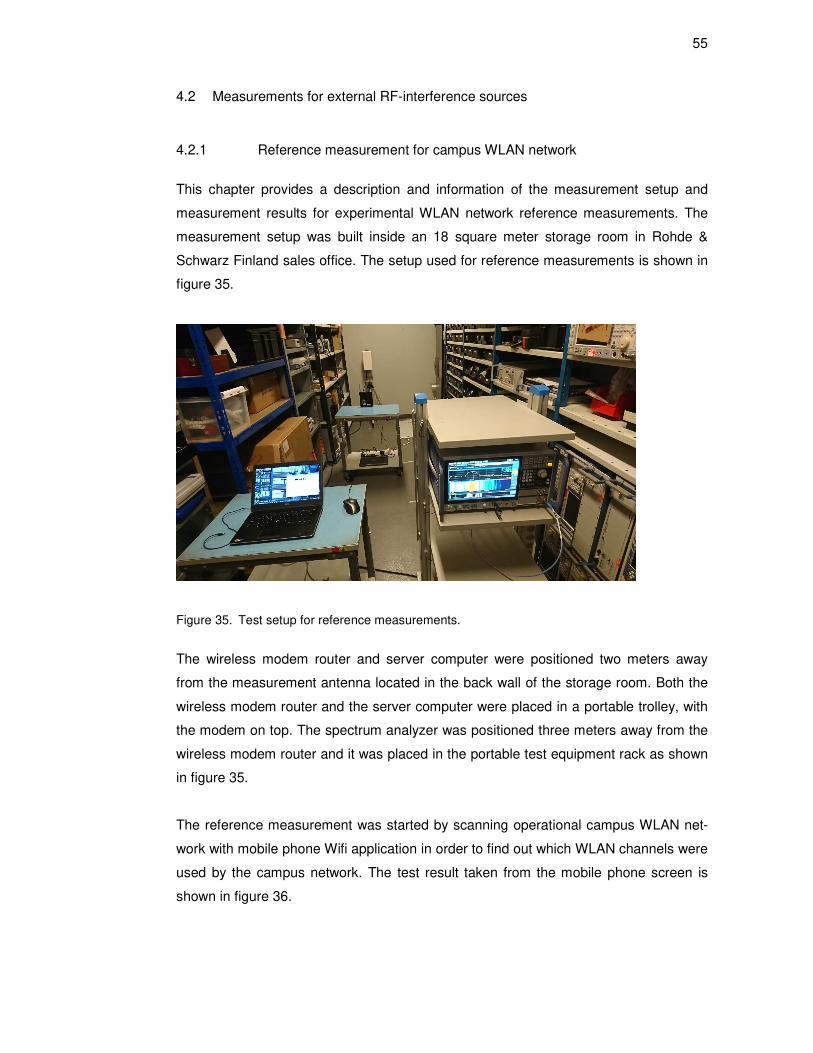
55
4.2 Measurements for external RF-interference sources
4.2.1 Reference measurement for campus WLAN network
This chapter provides a description and information of the measurement setup and
measurement results for experimental WLAN network reference measurements. The
measurement setup was built inside an 18 square meter storage room in Rohde &
Schwarz Finland sales office. The setup used for reference measurements is shown in
figure 35.
Figure 35. Test setup for reference measurements.
The wireless modem router and server computer were positioned two meters away
from the measurement antenna located in the back wall of the storage room. Both the
wireless modem router and the server computer were placed in a portable trolley, with
the modem on top. The spectrum analyzer was positioned three meters away from the
wireless modem router and it was placed in the portable test equipment rack as shown
in figure 35.
The reference measurement was started by scanning operational campus WLAN net-
work with mobile phone Wifi application in order to find out which WLAN channels were
used by the campus network. The test result taken from the mobile phone screen is
shown in figure 36.
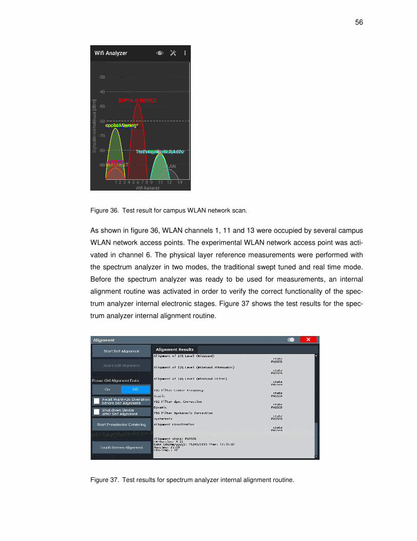
56
Figure 36. Test result for campus WLAN network scan.
As shown in figure 36, WLAN channels 1, 11 and 13 were occupied by several campus
WLAN network access points. The experimental WLAN network access point was acti-
vated in channel 6. The physical layer reference measurements were performed with
the spectrum analyzer in two modes, the traditional swept tuned and real time mode.
Before the spectrum analyzer was ready to be used for measurements, an internal
alignment routine was activated in order to verify the correct functionality of the spec-
trum analyzer internal electronic stages. Figure 37 shows the test results for the spec-
trum analyzer internal alignment routine.
Figure 37. Test results for spectrum analyzer internal alignment routine.

57
As shown in figure 37, the alignment routine was completed successfully without any
internal errors or warnings, the spectrum analyzer was ready to be used for measure-
ments.
The first series of spectrum analyzer measurements were started in the swept tuned
mode. The RMS detector and max hold trace function were selected in the spectrum
analyzer trace settings in order to measure the maximum power level and achieve
clean trace readings for active WLAN access point signals. Frequency range for the
measurement was set from 2401 MHz to 2495 MHz, thus covering a total occupied
bandwidth of 94 MHz for WLAN channels 1–14 operating in 2.4 GHz ISM frequency
band.
The Resolution Bandwidth (RBW) filter was set to 1 MHz and Video Bandwidth (VBW)
filter to 10 MHz, resulting in a short sweep time of 1.01 ms. The reference power level
was set to -20 dBm and internal attenuator to 0 dB position. In addition to the conven-
tional level versus frequency spectral trace display, a spectrogram display was activat-
ed. Figure 38 is showing the measurement results for swept tuned spectrum analyzer
reference measurement.
Figure 38. Swept tuned spectrum analyzer reference measurement results for experimental WLAN network. Two meters distance between measurement antenna and WLAN access point.
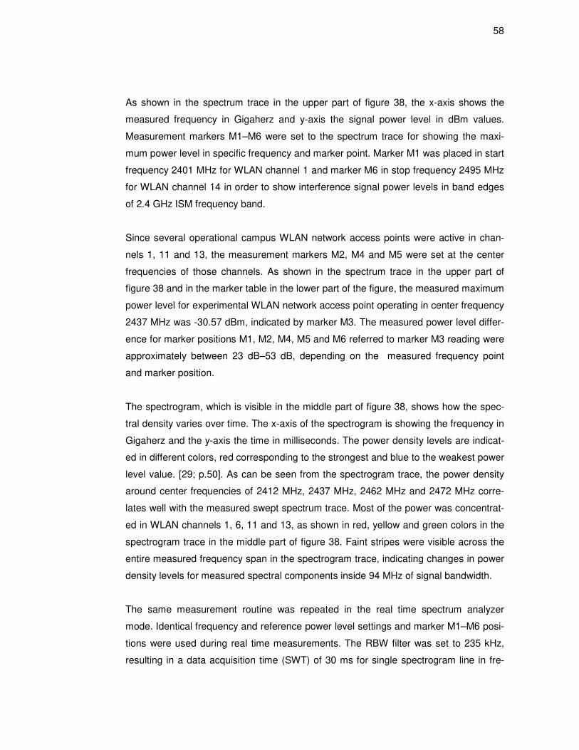
58
As shown in the spectrum trace in the upper part of figure 38, the x-axis shows the
measured frequency in Gigaherz and y-axis the signal power level in dBm values.
Measurement markers M1–M6 were set to the spectrum trace for showing the maxi-
mum power level in specific frequency and marker point. Marker M1 was placed in start
frequency 2401 MHz for WLAN channel 1 and marker M6 in stop frequency 2495 MHz
for WLAN channel 14 in order to show interference signal power levels in band edges
of 2.4 GHz ISM frequency band.
Since several operational campus WLAN network access points were active in chan-
nels 1, 11 and 13, the measurement markers M2, M4 and M5 were set at the center
frequencies of those channels. As shown in the spectrum trace in the upper part of
figure 38 and in the marker table in the lower part of the figure, the measured maximum
power level for experimental WLAN network access point operating in center frequency
2437 MHz was -30.57 dBm, indicated by marker M3. The measured power level differ-
ence for marker positions M1, M2, M4, M5 and M6 referred to marker M3 reading were
approximately between 23 dB–53 dB, depending on the measured frequency point
and marker position.
The spectrogram, which is visible in the middle part of figure 38, shows how the spec-
tral density varies over time. The x-axis of the spectrogram is showing the frequency in
Gigaherz and the y-axis the time in milliseconds. The power density levels are indicat-
ed in different colors, red corresponding to the strongest and blue to the weakest power
level value. [29; p.50]. As can be seen from the spectrogram trace, the power density
around center frequencies of 2412 MHz, 2437 MHz, 2462 MHz and 2472 MHz corre-
lates well with the measured swept spectrum trace. Most of the power was concentrat-
ed in WLAN channels 1, 6, 11 and 13, as shown in red, yellow and green colors in the
spectrogram trace in the middle part of figure 38. Faint stripes were visible across the
entire measured frequency span in the spectrogram trace, indicating changes in power
density levels for measured spectral components inside 94 MHz of signal bandwidth.
The same measurement routine was repeated in the real time spectrum analyzer
mode. Identical frequency and reference power level settings and marker M1–M6 posi-
tions were used during real time measurements. The RBW filter was set to 235 kHz,
resulting in a data acquisition time (SWT) of 30 ms for single spectrogram line in fre-
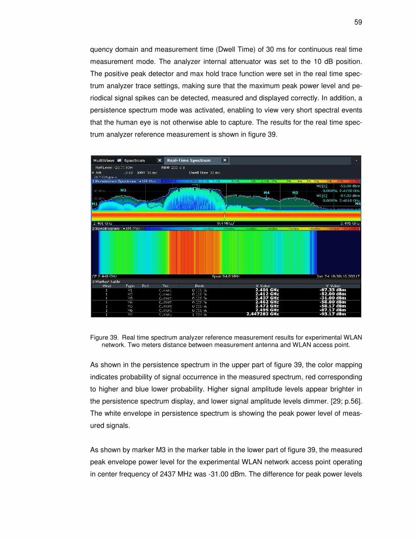
59
quency domain and measurement time (Dwell Time) of 30 ms for continuous real time
measurement mode. The analyzer internal attenuator was set to the 10 dB position.
The positive peak detector and max hold trace function were set in the real time spec-
trum analyzer trace settings, making sure that the maximum peak power level and pe-
riodical signal spikes can be detected, measured and displayed correctly. In addition, a
persistence spectrum mode was activated, enabling to view very short spectral events
that the human eye is not otherwise able to capture. The results for the real time spec-
trum analyzer reference measurement is shown in figure 39.
Figure 39. Real time spectrum analyzer reference measurement results for experimental WLAN network. Two meters distance between measurement antenna and WLAN access point.
As shown in the persistence spectrum in the upper part of figure 39, the color mapping
indicates probability of signal occurrence in the measured spectrum, red corresponding
to higher and blue lower probability. Higher signal amplitude levels appear brighter in
the persistence spectrum display, and lower signal amplitude levels dimmer. [29; p.56].
The white envelope in persistence spectrum is showing the peak power level of meas-
ured signals.
As shown by marker M3 in the marker table in the lower part of figure 39, the measured
peak envelope power level for the experimental WLAN network access point operating
in center frequency of 2437 MHz was -31.00 dBm. The difference for peak power levels
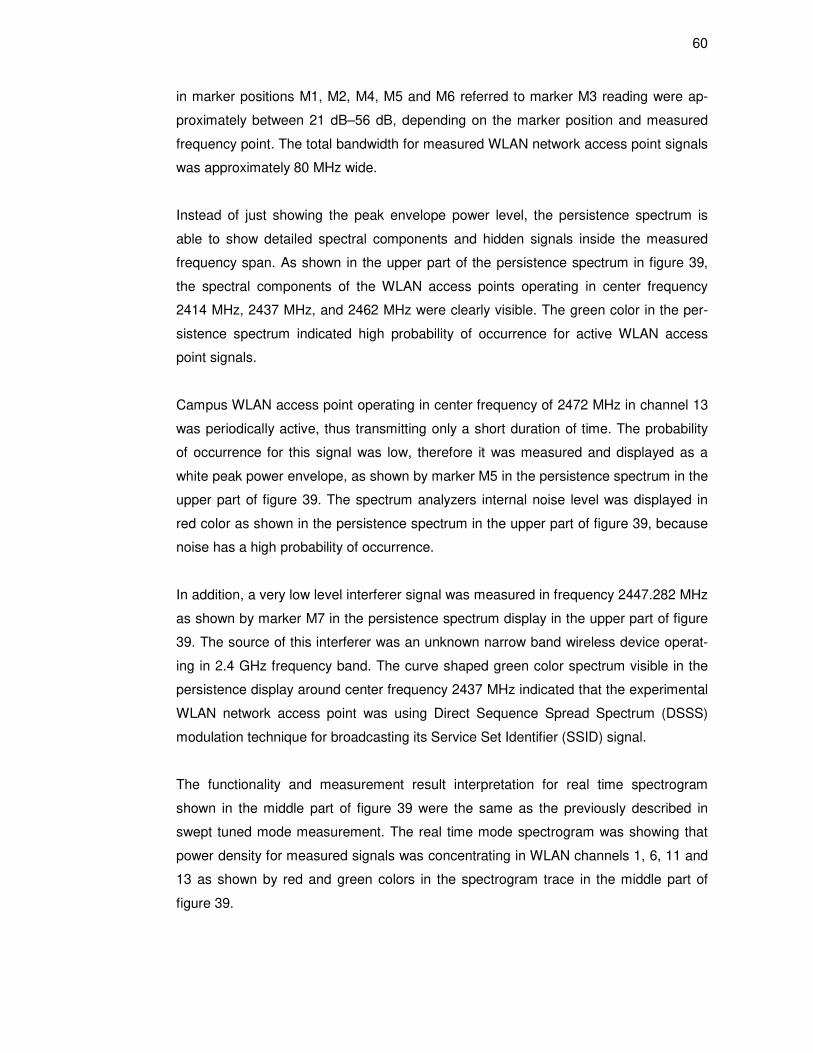
60
in marker positions M1, M2, M4, M5 and M6 referred to marker M3 reading were ap-
proximately between 21 dB–56 dB, depending on the marker position and measured
frequency point. The total bandwidth for measured WLAN network access point signals
was approximately 80 MHz wide.
Instead of just showing the peak envelope power level, the persistence spectrum is
able to show detailed spectral components and hidden signals inside the measured
frequency span. As shown in the upper part of the persistence spectrum in figure 39,
the spectral components of the WLAN access points operating in center frequency
2414 MHz, 2437 MHz, and 2462 MHz were clearly visible. The green color in the per-
sistence spectrum indicated high probability of occurrence for active WLAN access
point signals.
Campus WLAN access point operating in center frequency of 2472 MHz in channel 13
was periodically active, thus transmitting only a short duration of time. The probability
of occurrence for this signal was low, therefore it was measured and displayed as a
white peak power envelope, as shown by marker M5 in the persistence spectrum in the
upper part of figure 39. The spectrum analyzers internal noise level was displayed in
red color as shown in the persistence spectrum in the upper part of figure 39, because
noise has a high probability of occurrence.
In addition, a very low level interferer signal was measured in frequency 2447.282 MHz
as shown by marker M7 in the persistence spectrum display in the upper part of figure
39. The source of this interferer was an unknown narrow band wireless device operat-
ing in 2.4 GHz frequency band. The curve shaped green color spectrum visible in the
persistence display around center frequency 2437 MHz indicated that the experimental
WLAN network access point was using Direct Sequence Spread Spectrum (DSSS)
modulation technique for broadcasting its Service Set Identifier (SSID) signal.
The functionality and measurement result interpretation for real time spectrogram
shown in the middle part of figure 39 were the same as the previously described in
swept tuned mode measurement. The real time mode spectrogram was showing that
power density for measured signals was concentrating in WLAN channels 1, 6, 11 and
13 as shown by red and green colors in the spectrogram trace in the middle part of
figure 39.
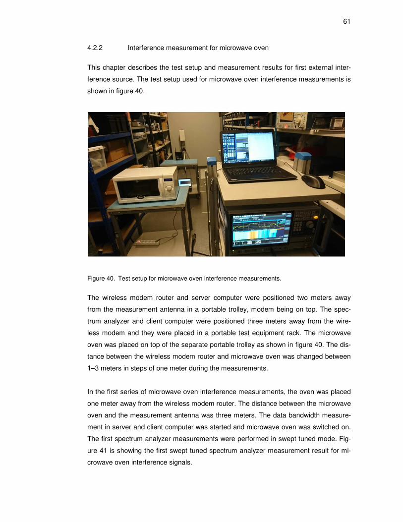
61
4.2.2 Interference measurement for microwave oven
This chapter describes the test setup and measurement results for first external inter-
ference source. The test setup used for microwave oven interference measurements is
shown in figure 40.
Figure 40. Test setup for microwave oven interference measurements.
The wireless modem router and server computer were positioned two meters away
from the measurement antenna in a portable trolley, modem being on top. The spec-
trum analyzer and client computer were positioned three meters away from the wire-
less modem and they were placed in a portable test equipment rack. The microwave
oven was placed on top of the separate portable trolley as shown in figure 40. The dis-
tance between the wireless modem router and microwave oven was changed between
1–3 meters in steps of one meter during the measurements.
In the first series of microwave oven interference measurements, the oven was placed
one meter away from the wireless modem router. The distance between the microwave
oven and the measurement antenna was three meters. The data bandwidth measure-
ment in server and client computer was started and microwave oven was switched on.
The first spectrum analyzer measurements were performed in swept tuned mode. Fig-
ure 41 is showing the first swept tuned spectrum analyzer measurement result for mi-
crowave oven interference signals.
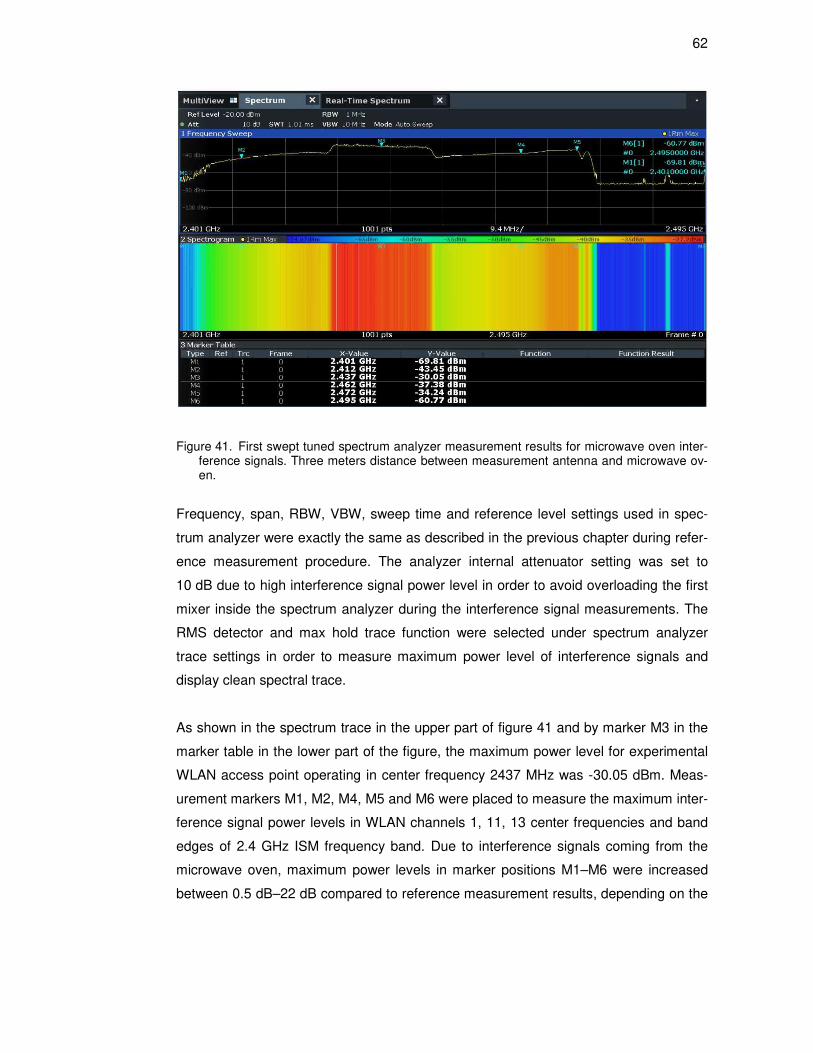
62
Figure 41. First swept tuned spectrum analyzer measurement results for microwave oven inter-ference signals. Three meters distance between measurement antenna and microwave ov-en.
Frequency, span, RBW, VBW, sweep time and reference level settings used in spec-
trum analyzer were exactly the same as described in the previous chapter during refer-
ence measurement procedure. The analyzer internal attenuator setting was set to
10 dB due to high interference signal power level in order to avoid overloading the first
mixer inside the spectrum analyzer during the interference signal measurements. The
RMS detector and max hold trace function were selected under spectrum analyzer
trace settings in order to measure maximum power level of interference signals and
display clean spectral trace.
As shown in the spectrum trace in the upper part of figure 41 and by marker M3 in the
marker table in the lower part of the figure, the maximum power level for experimental
WLAN access point operating in center frequency 2437 MHz was -30.05 dBm. Meas-
urement markers M1, M2, M4, M5 and M6 were placed to measure the maximum inter-
ference signal power levels in WLAN channels 1, 11, 13 center frequencies and band
edges of 2.4 GHz ISM frequency band. Due to interference signals coming from the
microwave oven, maximum power levels in marker positions M1–M6 were increased
between 0.5 dB–22 dB compared to reference measurement results, depending on the
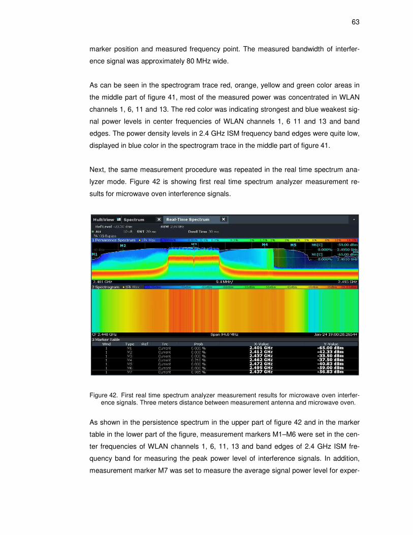
63
marker position and measured frequency point. The measured bandwidth of interfer-
ence signal was approximately 80 MHz wide.
As can be seen in the spectrogram trace red, orange, yellow and green color areas in
the middle part of figure 41, most of the measured power was concentrated in WLAN
channels 1, 6, 11 and 13. The red color was indicating strongest and blue weakest sig-
nal power levels in center frequencies of WLAN channels 1, 6 11 and 13 and band
edges. The power density levels in 2.4 GHz ISM frequency band edges were quite low,
displayed in blue color in the spectrogram trace in the middle part of figure 41.
Next, the same measurement procedure was repeated in the real time spectrum ana-
lyzer mode. Figure 42 is showing first real time spectrum analyzer measurement re-
sults for microwave oven interference signals.
Figure 42. First real time spectrum analyzer measurement results for microwave oven interfer-ence signals. Three meters distance between measurement antenna and microwave oven.
As shown in the persistence spectrum in the upper part of figure 42 and in the marker
table in the lower part of the figure, measurement markers M1–M6 were set in the cen-
ter frequencies of WLAN channels 1, 6, 11, 13 and band edges of 2.4 GHz ISM fre-
quency band for measuring the peak power level of interference signals. In addition,
measurement marker M7 was set to measure the average signal power level for exper-
64
imental WLAN access point operating in center frequency 2437 MHz. As shown in the
marker table in the lower part of figure 42, marker M3 indicates peak power level
-33.50 dBm and marker M7 average power level -56.83 dBm in frequency point 2437
MHz for WLAN access point operating in channel 6. Maximum power levels in marker
positions M1–M6 were increased between 2.5 dB–28 dB compared to reference meas-
urement results, depending on the marker position and measured frequency point.
Persistence spectrum functionality revealed that the bandwidth for interference signals
coming from the microwave oven was actually 94 MHz wide as shown in the persis-
tence spectrum trace in the upper part of figure 42. The red rectangular spectrum visi-
ble in the persistence display around center frequency 2437 MHz was indicating that
experimental WLAN network access point was using OFDM modulation technique for
data transmission.
The probability of occurrence for wideband interfering signal coming from the micro-
wave oven was high. This can be observed in the green color areas in the persistence
spectrum in the upper part of figure 42. In addition, a narrow band interference signal
was detected in the persistence spectrum as a green color spike between markers M4
and M5, and it was slightly shifting in the frequency axis during the operation of the
microwave oven. The source of this interference signal was the microwave oven’s
magnetron.
As displayed in the spectrogram trace in red, orange and yellow color areas in the mid-
dle part of figure 42, most of the power was concentrated in WLAN channels 1, 6, 11
and 13. Faint stripes visible across the entire spectrogram trace indicated changes in
power density levels for spectral components inside the measured frequency span. The
difference between real time spectrogram and swept tuned spectrogram was that real
time spectrogram was detecting quite high power level readings in band edges as
shown in the spectrogram trace in green and light blue colors in the middle part of fig-
ure 42. The reason for this is because bandwidth of microwave interference signals
was 94 MHz wide in reality.
The same measurement procedures for microwave oven interference signals were
repeated also in four and five meter distances between the measurement antenna and
the microwave oven. These measurements show similar test results for both meas-
urement distances. The peak power levels for interference signals were decreasing as
distance between measurement antenna and microwave oven was increasing, while

65
the bandwidth for interference signals remained the same. No other notable spurious
interferers were detected during the second and third swept tuned and real time spec-
trum analyzer measurements. The measurement results for the second and third mi-
crowave oven interference signal spectrum analyzer measurements are shown in Ap-
pendix 1.
4.2.3 Interference measurement for Bluetooth loudspeaker
This chapter describes the test setup and measurement results for the second external
interference source. The test setup used for Bluetooth loudspeaker interference meas-
urements is shown in figure 43.
Figure 43. Test setup for Bluetooth loudspeaker interference measurements.
As shown in figure 43, the wireless modem router and server computer were positioned
two meters away from the measurement antenna in a portable trolley, the modem be-
ing on top. The spectrum analyzer and client computer were positioned three meters
away from the wireless modem and they were placed in a portable test equipment rack.
Bluetooth loudspeaker was placed on top of the separate portable trolley. During the
Bluetooth loudspeaker interference measurements, the speaker was moved 1–3 me-
ters away from WLAN access point in steps of one meter. Exactly the same spectrum

66
analyzer settings and measurement procedures were used for performing Bluetooth
loudspeaker interference measurements as in case of the microwave oven.
In the first series of Bluetooth loudspeaker interference measurements, the speaker
was placed one meter away from the wireless modem router. The distance between
the loudspeaker and the measurement antenna was three meters. The data bandwidth
measurement in server and client computer was started and the speaker was activat-
ed. Figure 44 shows the first swept tuned interference signal measurement results for
Bluetooth loudspeaker.
Figure 44. First swept tuned spectrum analyzer measurement results for Bluetooth loudspeaker interference signals. Three meters distance between measurement antenna and Bluetooth loudspeaker.
As shown by marker M3 in the spectral trace and the marker table in figure 44, the
measured maximum power level for experimental WLAN access point operating in cen-
ter frequency 2437 MHz was -30.94 dBm. Measurement markers M1, M2, M4, M5 and
M6 were set to measure maximum power levels in WLAN channels 1, 11, 13 center
frequencies and band edges of 2.4 GHz ISM frequency band. Due to signals coming
from the Bluetooth loudspeaker, the maximum power levels in marker positions M1–M6
were increased between 15 dB–40 dB compared to reference measurement results,
depending on the marker position and measured frequency point. The measured
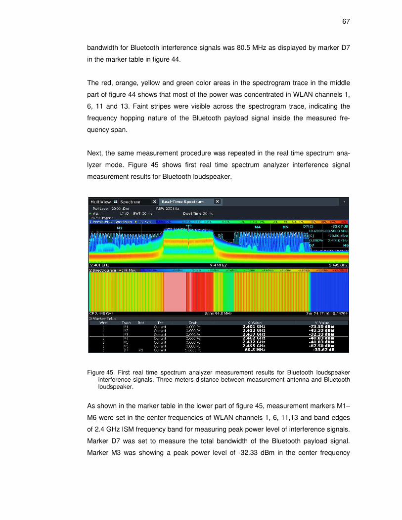
67
bandwidth for Bluetooth interference signals was 80.5 MHz as displayed by marker D7
in the marker table in figure 44.
The red, orange, yellow and green color areas in the spectrogram trace in the middle
part of figure 44 shows that most of the power was concentrated in WLAN channels 1,
6, 11 and 13. Faint stripes were visible across the spectrogram trace, indicating the
frequency hopping nature of the Bluetooth payload signal inside the measured fre-
quency span.
Next, the same measurement procedure was repeated in the real time spectrum ana-
lyzer mode. Figure 45 shows first real time spectrum analyzer interference signal
measurement results for Bluetooth loudspeaker.
Figure 45. First real time spectrum analyzer measurement results for Bluetooth loudspeaker interference signals. Three meters distance between measurement antenna and Bluetooth loudspeaker.
As shown in the marker table in the lower part of figure 45, measurement markers M1–
M6 were set in the center frequencies of WLAN channels 1, 6, 11,13 and band edges
of 2.4 GHz ISM frequency band for measuring peak power level of interference signals.
Marker D7 was set to measure the total bandwidth of the Bluetooth payload signal.
Marker M3 was showing a peak power level of -32.33 dBm in the center frequency

68
2437 MHz for WLAN access point operating in channel 6. Marker D7 indicated that the
measured bandwidth for Bluetooth payload signal was 80.5 MHz, as shown in the
marker table in the lower part of figure 45. Maximum peak power levels in marker posi-
tions M1–M6 were increased between 9 dB–18 dB compared to reference measure-
ment results, depending on the marker position and measured frequency point.
The probability of occurrence for Bluetooth signal peak power levels were quite low.
This can be observed in the dark blue color areas in the persistence spectrum, as
shown the upper part of figure 45. The frequency hopping nature of the Bluetooth sig-
nal payload could clearly be identified from the narrowband blue colored sub-channels,
visible in the persistence spectrum as shown in the upper part of figure 45.
In addition, narrow green signal spikes were visible around marker positions M2, M4
and M5 as shown in the persistence spectrum display in the upper part of figure 45.
The source of these spikes were campus WLAN network access points transmitting in
WLAN channels 1, 11 and 13. The red, orange, yellow and green color areas in the
spectrogram display in the middle part of figure 45 indicated that most of the power
was concentrated in WLAN channels 1, 6, 11 and 13. Faint visible stripes in the spec-
trogram were indicating that the measured interference signal came from a frequency
hopping device.
The same measurement procedures for Bluetooth loudspeaker interferences were also
repeated in four and five meter distances between the measurement antenna and the
Bluetooth device. These measurements show similar test results for both measurement
distances. The peak power level of interference signals were decreasing as the dis-
tance between measurement antenna and Bluetooth loudspeaker was increasing,
while the bandwidth of interference signals remained the same. No other spurious in-
terference signals were detected during the second and third swept tuned and real time
spectrum analyzer measurements. The measurement results for the second and third
Bluetooth loudspeaker interference signal spectrum analyzer measurements are shown
in Appendix 2.

69
4.3 Recording of WLAN network data bandwidth
4.3.1 Reference data bandwidth measurement
In this chapter, the test setup for the reference data bandwidth measurement inside the
experimental WLAN network and measured test results are described. During the ref-
erence measurement, both of the external interference sources, i.e. the microwave
oven and the Bluetooth loudspeaker, were switched off. Test setup used for the refer-
ence measurement is shown in figure 46.
Figure 46. Test setup for reference data bandwidth measurement.
The wireless modem router and server computer were positioned 2 meters away from
the back wall of the storage room. They were placed in the portable trolley, the modem
being on the top level. The wireless modem router was set to operate in the center fre-
quency of 2437 MHz in WLAN channel 6. The wireless client computer was positioned
3 meters away from the wireless modem and it was placed on top of another portable
trolley as shown in figure 46.
The reference data bandwidth was measured and recorded with the network perfor-
mance software tool jPerf, which is able to create network traffic for data bandwidth
measurements. The software can be set to run in two main modes, the server and the
client. It can be configured to create network traffic by using the Transmission Control
Protocol (TCP) or the User Datagram Protocol (UDP). In order to run a successful data

70
bandwidth measurement, the IP-addresses of both the server and the client computers
need to be set to operate inside the same local area subnetwork.
Separate copies of jPerf software were installed for both the server and the client com-
puters. The server computers jPerf software was started in server mode and it was
using the server computers’ network interface card IP-address for network communica-
tion. No further configurations for server computer were needed, it was ready for
measurements waiting for client computer connection.
The client computers jPerf software was started in client mode. TCP test parameters
for data bandwidth measurement was set for creating network traffic. The server com-
puter IP-address was set to client computers jPerf software. Figure 47 shows the appli-
cation and transport layer settings used in the client computers jPef software during the
reference data bandwidth measurement.
Figure 47. Application and transport layer settings for client computers jPerf software.

71
As shown in figure 47, the transmit time for generated data streams was set to 180
seconds. The reporting interval for test results was set to 1 second, the used TCP test
port to 5001 and output format Mbit/s. During the data bandwidth measurements, the
client computer jPerf software was generating TCP data packages in order to create
network traffic. The buffer length, TCP window size, max segment size and TCP no
delay settings were left at their default values. After all test parameters were set for the
server and client computers, the actual reference data bandwidth measurement was
performed. Figure 48 shows the test result for reference data bandwidth measurement.
Figure 48. Measurement result for reference data bandwidth, external interferers switched off.
In figure 48, the x-axis presents the total measurement time in seconds with step size
of twenty seconds and the y-axis the measured data bandwidth in Mbit/s for experi-
mental WLAN network access point operating in channel 6. The server computer jPerf
software was recording 83,2 Mbit/s as average data bandwidth value within 180 sec-
onds of measurement time. The theoretical top speed for wireless network interface
card supporting 802.11n protocol is up to 600 Mbit/s, but in practice a data bandwidth
of approximately 80 Mbit/s–150 Mbit/s can be achieved in public WLAN networks most
of the time.
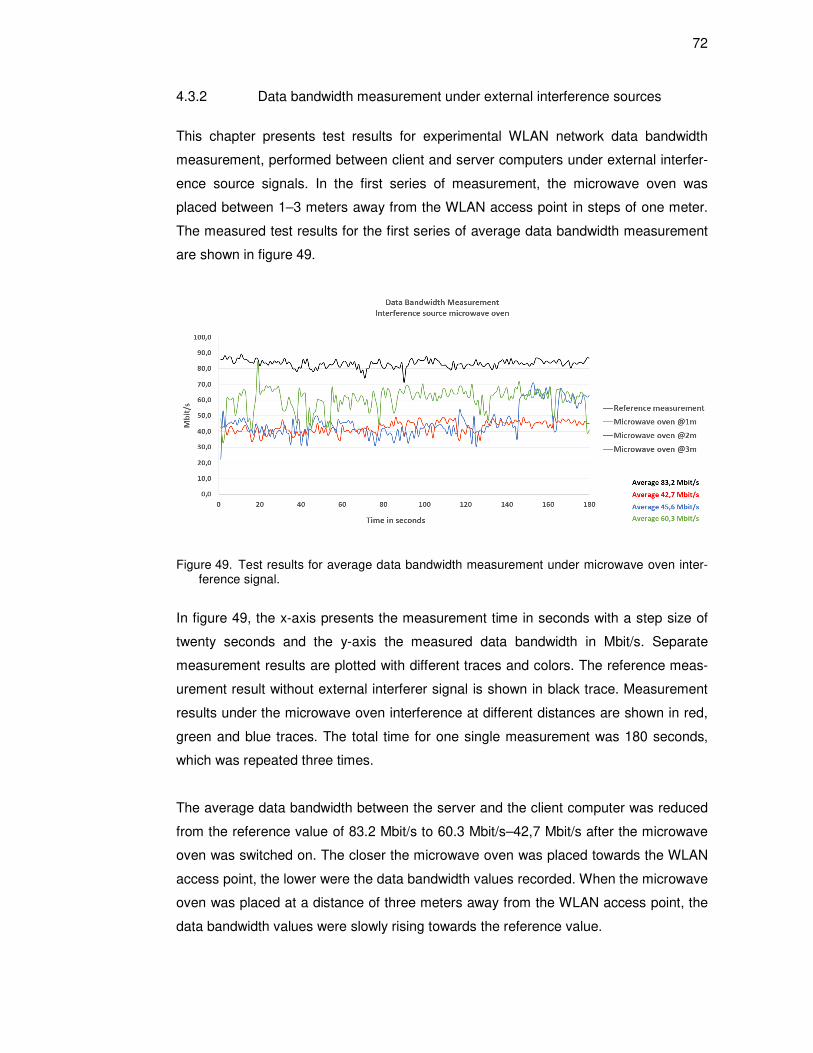
72
4.3.2 Data bandwidth measurement under external interference sources
This chapter presents test results for experimental WLAN network data bandwidth
measurement, performed between client and server computers under external interfer-
ence source signals. In the first series of measurement, the microwave oven was
placed between 1–3 meters away from the WLAN access point in steps of one meter.
The measured test results for the first series of average data bandwidth measurement
are shown in figure 49.
Figure 49. Test results for average data bandwidth measurement under microwave oven inter-ference signal.
In figure 49, the x-axis presents the measurement time in seconds with a step size of
twenty seconds and the y-axis the measured data bandwidth in Mbit/s. Separate
measurement results are plotted with different traces and colors. The reference meas-
urement result without external interferer signal is shown in black trace. Measurement
results under the microwave oven interference at different distances are shown in red,
green and blue traces. The total time for one single measurement was 180 seconds,
which was repeated three times.
The average data bandwidth between the server and the client computer was reduced
from the reference value of 83.2 Mbit/s to 60.3 Mbit/s–42,7 Mbit/s after the microwave
oven was switched on. The closer the microwave oven was placed towards the WLAN
access point, the lower were the data bandwidth values recorded. When the microwave
oven was placed at a distance of three meters away from the WLAN access point, the
data bandwidth values were slowly rising towards the reference value.

73
As shown by the green and blue traces in figure 49, a few high spikes in recorded val-
ues were observed when the microwave oven was placed two and three meters away
from the WLAN access point. The red trace indicates that the measured data band-
width was quite flat over the entire measurement time while the microwave oven was
placed one meter away from the WLAN access point.
In the second series of data bandwidth measurements, the Bluetooth loudspeaker was
placed between 1–3 meters away from the WLAN access point in steps of one meter.
Figure 50 shows the measured test results for the second series of average data
bandwidth measurement.
Figure 50. Test results for average data bandwidth measurements under Bluetooth loudspeaker interference signal.
As shown in figure 50 by the red, green and blue traces, the average data bandwidth
between the server and the client computer was slightly reduced from the reference
value of 83.2 Mbit/s to 75.9 Mbit/s–79,0 Mbit/s after the Bluetooth loudspeaker was
activated. The closer the loudspeaker was placed towards the experimental WLAN
access point, the lower were the data bandwidth values recorded. All recorded traces
were quite flat, no large spikes were observed during the Bluetooth loudspeaker data
bandwidth measurements.
74
4.4 Analysis of measured data
4.4.1 External RF-interference signals
In this chapter, the final test results for the microwave oven and Bluetooth loudspeaker
RF-interference signal measurements are shown and analyzed. The spectrum analyzer
measurements for physical layer interference signals were performed in swept tuned
and real time modes in order to illustrate the typical differences between these two
measurement technologies. During the measurements, the antenna was placed in the
back wall of the storage room. As a general rule, an antenna has to be placed under
the far field condition of measured electromagnetic wave in order to get reliable meas-
urement results. The wavelength of 2.4 GHz ISM frequency band signals in free space
is approximately 12 centimeters. As the physical dimension of the Aerial measurement
antenna panel was significantly larger compared to the wave length, the distance be-
tween the measurement antenna and the interference signal sources was chosen to be
between 2–5 meters in order to meet the far field condition in all measurement posi-
tions.
The physical layer connection of WLAN devices is based on the Carrier Sense Multiple
Access with Collision Avoidance (CSMA/CA) technique. Devices are transmitting for a
short duration of time and only when the transmission channel is free, while no other
transmissions are detected in the same channel. In the swept tuned mode, the spec-
trum analyzer is sweeping through the selected frequency span, thus resulting in cer-
tain overall sweep time depending on the selected frequency span, resolution and vid-
eo bandwidth settings. In practice, the analyzer is not able to show reliable maximum
power level readings for the WLAN signal source if wrong trace, sweep time, RBW or
VBW settings are selected. In order to get clear trace readings, the max hold trace
function, 1 MHz RBW, 10 MHz VBW and 1.01 ms sweep time settings were used dur-
ing the swept tuned spectrum analyzer measurements.
The swept tuned measurement typically takes a long measurement time for catching
short duration signals, such as fast transient spikes at the band edges of a wide band
interference signal. During the 180 seconds of total measurement time, the swept
tuned spectrum analyzer was only showing a 80 MHz bandwidth for microwave oven
interferences, but in reality the bandwidth was 94 MHz wide as later measured in real
time mode. It would have taken several tens of minutes or even hours of measurement

75
time just to show the total bandwidth of 94 MHz interference signal in swept tuned
mode. A conventional swept tuned spectrum analyzer is not the ideal measurement
device for showing separate spectral components inside the measured frequency band
of short duration signals such as spurious signals or Bluetooth device frequency hop-
ping payload signals. In order to recognize the spectral signature of frequency hopping
devices in swept tuned mode, the usage of spectrogram is highly recommended. Inter-
ference signals coming from frequency hopping devices can be identified as stripes,
shown by the different colors in the spectrogram trace.
The most precise measurement technology for interference signal hunting is real time
spectrum analysis. In real time mode, the spectrum analyzer captures the bandwidth of
800 MHz signal at once and calculates the spectrum with the aid of FFT algorithms
inside powerful and fast Field Programmable Gate Array (FPGA) circuits. Real time
spectrum analyzer is capable of showing measurement results within few micro sec-
onds of time in the display of the analyzer. It is also capable of showing short duration
signals and separate spectral components inside the entire measured frequency span.
The spectrum signature of frequency hopping devices such as Bluetooth signal pay-
load and other narrow and wideband external interferences can be easily displayed in
the real time persistence spectrum.
Three separate real time interference measurements for both the microwave oven and
the Bluetooth loudspeaker were performed in six different frequency points in the 2.4
GHz ISM frequency band. Figure 51 shows summary test results for the microwave
oven’s real time peak power interference measurements.
Figure 51. Summary of real time spectrum analyzer peak power measurement results for mi-crowave oven interferences.

76
In figure 51, the x-axis shows the measured frequency in Megahertz and the y-axis the
signal peak power level in dBm value at a specific frequency point. Every frequency
point contains four bars indicating measurements performed in different distances and
the measurement marker used during the measurement procedure. The yellow bar
represents the reference measurement performed for the experimental WLAN access
point, positioned two meters away from measurement antenna. The blue, orange and
grey bars represent external interference signal measurements for the microwave ov-
en, positioned three, four and five meters away from the measurement antenna. The
highest peak power levels for reference measurement were found in frequencies 2412
MHz, 2437 MHz, 2462 MHz and 2472 MHz as shown by the yellow bars in figure 51.
The peak power level was very low in band edges 2401 MHz and 2495 MHz frequen-
cies during reference measurement. The bandwidth for the microwave oven interfer-
ence signal was 94 MHz wide, covering all WLAN channels in the 2.4 GHz ISM fre-
quency band.
The measured peak power level in the center frequency of 2437 MHz was almost con-
stant in all distances as shown by the blue, orange and grey bars in figure 51. The in-
terference signal coming from the microwave oven was strongest in a measurement
distance of three meters away from the measurement antenna, as shown by blue bars
in most of the frequency points. When the distance between the microwave oven and
the measurement antenna increased, the measured peak power level decreased in all
frequency points except center frequency 2437 MHz. The microwave oven created less
interference with the WLAN access point physical layer signal when the oven was
moved further away from the access point.
Figure 52 shows the summary test results for the Bluetooth loudspeaker’s real time
peak power interference measurements.
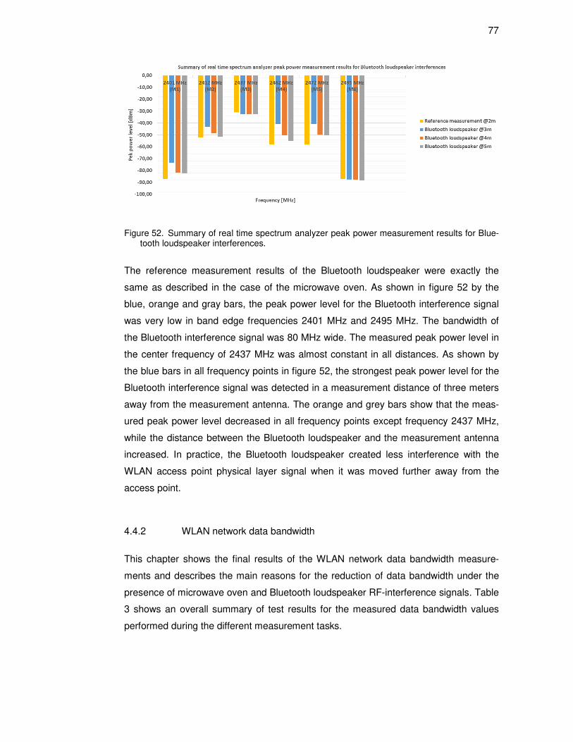
77
Figure 52. Summary of real time spectrum analyzer peak power measurement results for Blue-tooth loudspeaker interferences.
The reference measurement results of the Bluetooth loudspeaker were exactly the
same as described in the case of the microwave oven. As shown in figure 52 by the
blue, orange and gray bars, the peak power level for the Bluetooth interference signal
was very low in band edge frequencies 2401 MHz and 2495 MHz. The bandwidth of
the Bluetooth interference signal was 80 MHz wide. The measured peak power level in
the center frequency of 2437 MHz was almost constant in all distances. As shown by
the blue bars in all frequency points in figure 52, the strongest peak power level for the
Bluetooth interference signal was detected in a measurement distance of three meters
away from the measurement antenna. The orange and grey bars show that the meas-
ured peak power level decreased in all frequency points except frequency 2437 MHz,
while the distance between the Bluetooth loudspeaker and the measurement antenna
increased. In practice, the Bluetooth loudspeaker created less interference with the
WLAN access point physical layer signal when it was moved further away from the
access point.
4.4.2 WLAN network data bandwidth
This chapter shows the final results of the WLAN network data bandwidth measure-
ments and describes the main reasons for the reduction of data bandwidth under the
presence of microwave oven and Bluetooth loudspeaker RF-interference signals. Table
3 shows an overall summary of test results for the measured data bandwidth values
performed during the different measurement tasks.
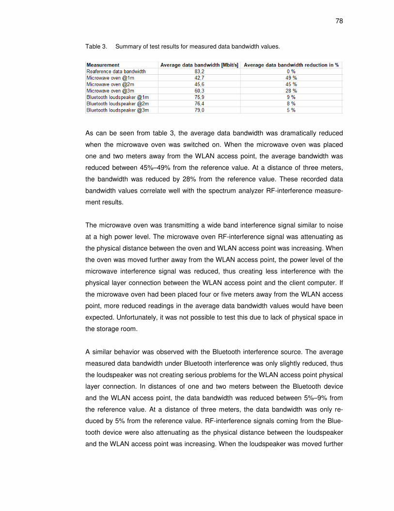
78
Table 3. Summary of test results for measured data bandwidth values.
As can be seen from table 3, the average data bandwidth was dramatically reduced
when the microwave oven was switched on. When the microwave oven was placed
one and two meters away from the WLAN access point, the average bandwidth was
reduced between 45%–49% from the reference value. At a distance of three meters,
the bandwidth was reduced by 28% from the reference value. These recorded data
bandwidth values correlate well with the spectrum analyzer RF-interference measure-
ment results.
The microwave oven was transmitting a wide band interference signal similar to noise
at a high power level. The microwave oven RF-interference signal was attenuating as
the physical distance between the oven and WLAN access point was increasing. When
the oven was moved further away from the WLAN access point, the power level of the
microwave interference signal was reduced, thus creating less interference with the
physical layer connection between the WLAN access point and the client computer. If
the microwave oven had been placed four or five meters away from the WLAN access
point, more reduced readings in the average data bandwidth values would have been
expected. Unfortunately, it was not possible to test this due to lack of physical space in
the storage room.
A similar behavior was observed with the Bluetooth interference source. The average
measured data bandwidth under Bluetooth interference was only slightly reduced, thus
the loudspeaker was not creating serious problems for the WLAN access point physical
layer connection. In distances of one and two meters between the Bluetooth device
and the WLAN access point, the data bandwidth was reduced between 5%–9% from
the reference value. At a distance of three meters, the data bandwidth was only re-
duced by 5% from the reference value. RF-interference signals coming from the Blue-
tooth device were also attenuating as the physical distance between the loudspeaker
and the WLAN access point was increasing. When the loudspeaker was moved further
79
away from the WLAN access point, the power level of the Bluetooth interference signal
was reduced, thus interfering less with WLAN access point physical layer connection.
Bluetooth devices are operating in ISM frequency band between frequencies
2400 MHz–2485 MHz. The bandwidth for Bluetooth payload signal is typically 80 MHz
wide, depending on the used device type. Bluetooth devices are using Frequency Hop-
ping Spread Spectrum (FHSS) technology, usually at a rate of 1600 hops per second.
Bluetooth transmission is spread over 79 separate sub-channels, the bandwidth for
each channel is 1 MHz wide. As a consequence, Bluetooth devises are creating less
RF-interferences for WLAN devices operating in same ISM frequency band. The max-
imum power level of each designated sub-channels is only present for a short period of
time in the frequency spectrum and the bandwidth of one sub-channel is quite narrow.
Modern WLAN access points are capable of handling short time physical layer RF-
interferences quite well.
5 Practical implications for hospital WLAN network environment
Setting up a WLAN network in the hospital building, network administrators need to
consider few basic preparation steps before actual network is deployed to a fully func-
tional state. The minimum recommended five steps for designing and building a hospi-
tal WLAN network are described below.
• Proper site survey
• Frequency planning for the WLAN access points and selection of enter-prise controller
• Setting up the network
• Network security planning
• Network testing
In the first step, it is very important to perform a proper site survey for the hospital
building before network deployment. The person in charge must ensure effective
WLAN coverage and excellent Quality of Service (QoS) and minimize harm of RF inter-
ferences, which could be causing problems for the network performance. A site sur-
veyor must use up-to-date blueprints to optimize the network efficiency in all areas of
the building. [16; p.4]
80
The second step is frequency planning for the WLAN access points and selection of
the enterprise controller. Modern technology WLAN access points can be configured to
broadcast at 2.4 GHz or 5 GHz frequency bands. The 2.4 GHz frequency band is more
crowded because of the volume of devices using that band. The cell size is smaller in
the 5 GHz frequency band due to the shorter wave length and higher RF signal attenu-
ation. Any clinical device that is not transmitting life critical network traffic should be
designed to operate in the 2.4 GHz frequency band. All devices that are transmitting
life critical network traffic should be placed in operation on the 5 GHz frequency band in
order to enable a higher data rate in a less congested frequency band. [16; p.6]
Sensitive data is frequently transmitted in hospitals, therefore an enterprise grade net-
work infrastructure must be used. Enterprise graded WLAN access points offer better
security features, centralized user control and a larger set of different technical features
than normal home and business office access points. Also redundancy and self healing
capabilities are important features for life critical wireless medical network devices. [16;
p.6]
The third step is setting up the network. A separation of different data traffic on multiple
Virtual Local Area Networks (VLAN) ensures important and secure network communi-
cations and network segmentation. Proper VLAN access control measures must be
used in order to control the devices and user access for different areas of local area
network. Separate VLANs should be configured for hospital staff, private personal de-
vices, guests and clinical and medical devices in order to enhance network security.
The most important security feature is to separate guests from sensitive medical and
clinical information data. [16; p.6]
All personal wireless devices of guests and the hospital staff should be configured to
operate in the 2.4 GHz frequency band in order to assure high quality and high data
throughput for important life-critical wireless medical devices. Uninterrupted connection
is a key factor for life-critical and clinical wireless devices. Consumer devices, such as
smart phones, microwave ovens, Bluetooth devices, laptops and tablets, are all operat-
ing in the 2.4 GHz ISM band. All of these devices are potential RF interference sources
for medical devices operating in same frequency band. [16; p.6]
All life-critical hospital wireless devices should be placed in operation to the less con-
gested 5 GHz frequency band in order to secure robust transmission of secured data. It
81
is not recommended to use Dynamic Frequency Selection (DFS) functionality in hospi-
tal 5 GHz WLAN access points. DFS could be causing up to two seconds loss in life
critical medical device data transmission every time when an access point is scanning
for a new available RF channel. [16; p.6]
Modern hospital WLAN networks must also be able to transmit robust voice and video
data. Quality of Service (QoS) settings allows hierarchy and prioritization to be set for
specified traffic. QoS is typically implemented in VLAN level to improve throughput of
the system. Four levels of QoS packet prioritization is typically used when planning the
network. These are in order of significance Voice, Video, Best effort and Background
network traffic. Best effort is usually the default setting in WLAN hotspots, whereas
background priority is normally used for maintenance purposes. The manager in
charge must decide which VLAN traffic is most important and has the highest priority to
be processed first. It is recommended to switch off the QoS packet prioritization for
guest VLANs. All guest data connections should be treated as equal and to be handled
by using the first-in first-out principle for the network access. [16; p.7]
Planning and optimizing device roaming is an important part when setting up the net-
work. As a general rule, a roaming plan for 5 GHz band should be optimized first and
then set the transmit power of the 2.4 GHz WLAN hotspots to match the 5 GHz hotspot
cell size. It is highly recommended that WLAN devices used in hospitals should support
customization for roaming settings. This ability allows setting to be set in device level in
order to improve connectivity to the network. Typical customizable settings are low sig-
nal threshold, positive change in signal strength and minimum period of time before a
devise can roam back to previous access point. As a general rule, a mobile WLAN de-
vice should be able to roam faster than stationary devises. Every hospital has unique
physical environment and Information Technology (IT) requirements, therefore each
settings has to be planned at an individual device level, according to hospital IT policy.
[16; p.8]
The fourth step is network security planning. When transmitting sensitive data in a hos-
pital WLAN network, security settings must be set at a strong level. It is highly recom-
mended to use a high level of security protocols and encryption, such as Wi-Fi Protect-
ed Access II with advanced Encryption Standard (WPA2-AES). In addition to WPA2-
AES, an Extensible Authentication Protocol (EAP), i.e. authentication with certificates
should be in use. This requires the user to provide credentials before accessing the

82
network. In order to gain more security to network, separate VLANs need to be set for
guest access, staff devices and life-critical devices or sensitive information. [16; p.9]
The fifth step is network testing, which is recommend to be performed when initially
setting up the network, a new device is added, a physical attribute of the original site
survey has changed or a new version of firmware code is installed into the WLAN de-
vices. Minimum recommended test procedures should include tests for channel over-
lap, measurements for WLAN coverage and testing the wireless devices against secu-
rity breaches. When the hospital network is set up initially, a proper site survey has to
be performed. Access points are placed in the building according to results of the site
survey. A used case of each specific wireless devices should be carefully planned, and
tested in its intended normal operating environment and defined parameters. [16; p.10]
A usage of a spectrum analyzer is highly recommended in order to find sources of ex-
ternal RF-interferences. When an interference source is located, it should be plotted in
the blueprint, and the WLAN channels affected by the interference should be noted.
Based on the spectrum analysis findings, a placement of access points can begin and
planning of optimized cell size and data throughput can be performed. For difficult in-
door areas, specialized antennas can be used in order to maximize required coverage
requirements. [16; p.4]
6 Proposed actions and suggestions
The detection of external interference signals and their sources is an essential phase in
WLAN network design when planning and monitoring network Quality of Service (QoS)
parameters. Data bandwidth measurement alone does not reveal the overall condition
of the network. The physical layer signals also need to be verified in order to get a full
picture of the network performance. The best tool for performing physical layer RF-
signal measurements is a spectrum analyzer. There are many commercial applications
and devices available for this purpose. It is highly recommended to make a solid plan
for performing spectrum analyzer measurements in WLAN network. Some of the basic
steps for such a plan are listed below.
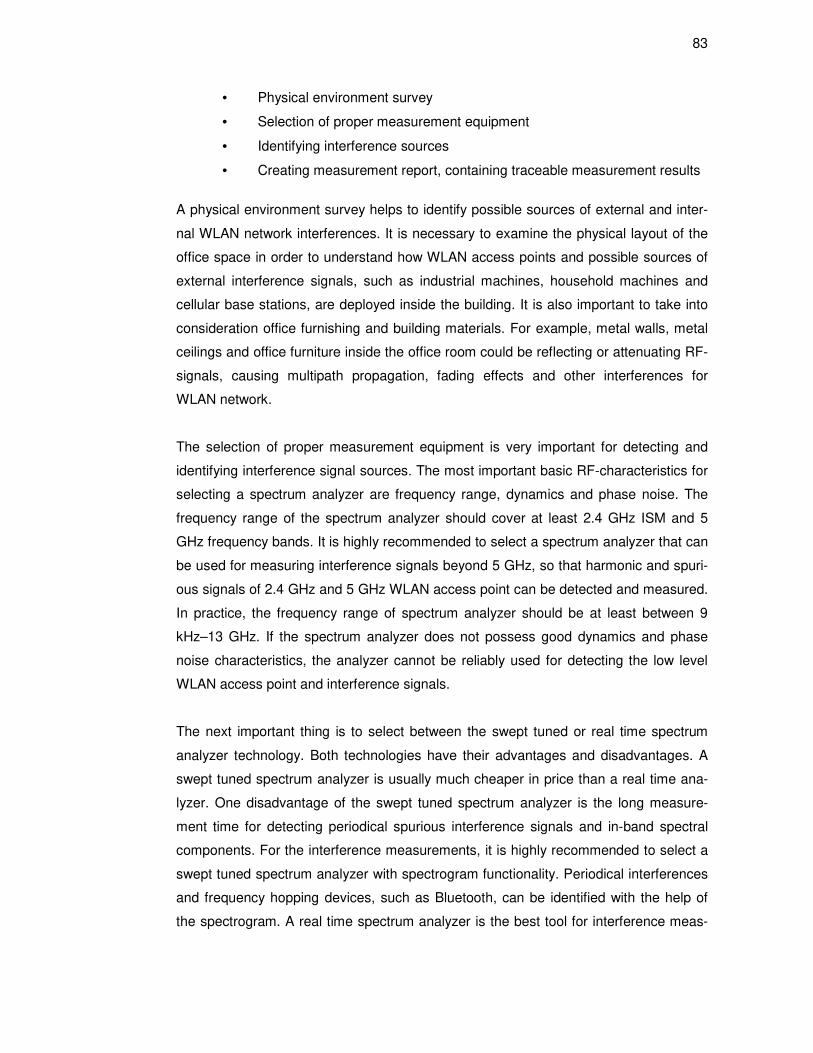
83
• Physical environment survey
• Selection of proper measurement equipment
• Identifying interference sources
• Creating measurement report, containing traceable measurement results
A physical environment survey helps to identify possible sources of external and inter-
nal WLAN network interferences. It is necessary to examine the physical layout of the
office space in order to understand how WLAN access points and possible sources of
external interference signals, such as industrial machines, household machines and
cellular base stations, are deployed inside the building. It is also important to take into
consideration office furnishing and building materials. For example, metal walls, metal
ceilings and office furniture inside the office room could be reflecting or attenuating RF-
signals, causing multipath propagation, fading effects and other interferences for
WLAN network.
The selection of proper measurement equipment is very important for detecting and
identifying interference signal sources. The most important basic RF-characteristics for
selecting a spectrum analyzer are frequency range, dynamics and phase noise. The
frequency range of the spectrum analyzer should cover at least 2.4 GHz ISM and 5
GHz frequency bands. It is highly recommended to select a spectrum analyzer that can
be used for measuring interference signals beyond 5 GHz, so that harmonic and spuri-
ous signals of 2.4 GHz and 5 GHz WLAN access point can be detected and measured.
In practice, the frequency range of spectrum analyzer should be at least between 9
kHz–13 GHz. If the spectrum analyzer does not possess good dynamics and phase
noise characteristics, the analyzer cannot be reliably used for detecting the low level
WLAN access point and interference signals.
The next important thing is to select between the swept tuned or real time spectrum
analyzer technology. Both technologies have their advantages and disadvantages. A
swept tuned spectrum analyzer is usually much cheaper in price than a real time ana-
lyzer. One disadvantage of the swept tuned spectrum analyzer is the long measure-
ment time for detecting periodical spurious interference signals and in-band spectral
components. For the interference measurements, it is highly recommended to select a
swept tuned spectrum analyzer with spectrogram functionality. Periodical interferences
and frequency hopping devices, such as Bluetooth, can be identified with the help of
the spectrogram. A real time spectrum analyzer is the best tool for interference meas-
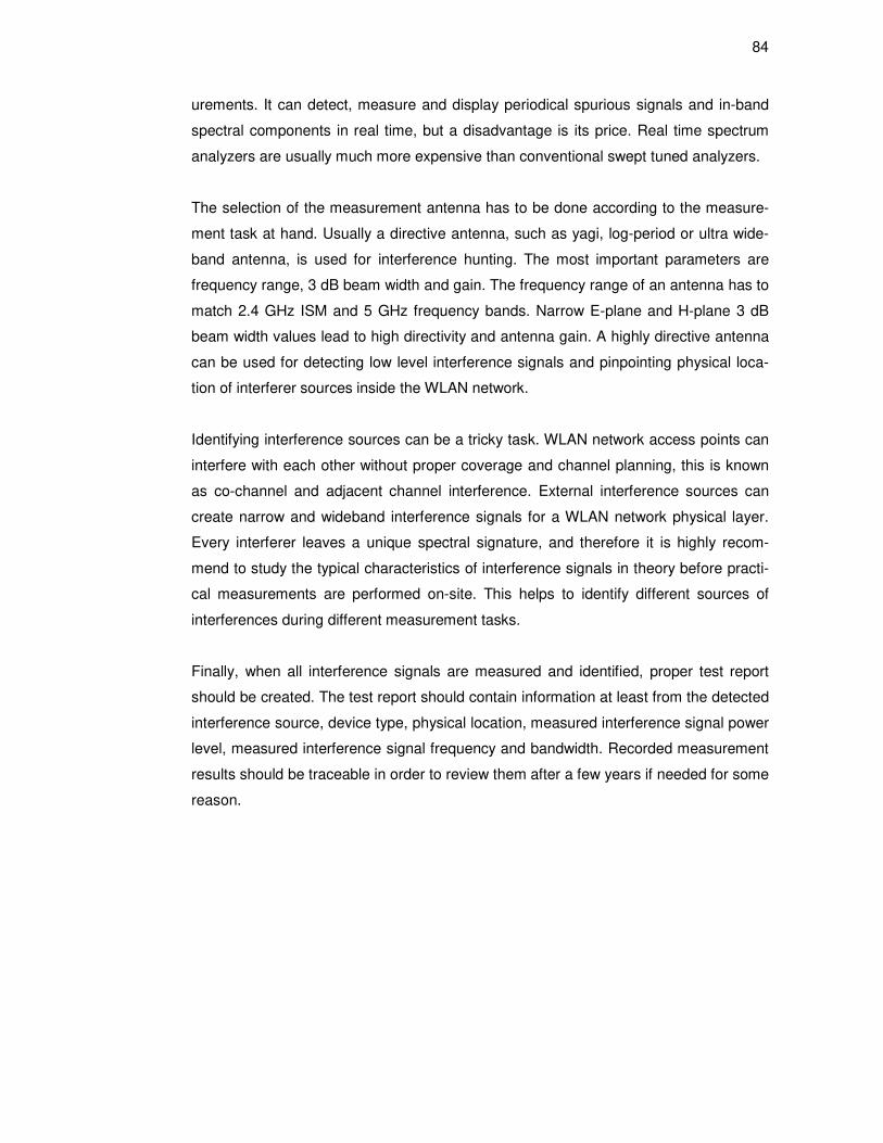
84
urements. It can detect, measure and display periodical spurious signals and in-band
spectral components in real time, but a disadvantage is its price. Real time spectrum
analyzers are usually much more expensive than conventional swept tuned analyzers.
The selection of the measurement antenna has to be done according to the measure-
ment task at hand. Usually a directive antenna, such as yagi, log-period or ultra wide-
band antenna, is used for interference hunting. The most important parameters are
frequency range, 3 dB beam width and gain. The frequency range of an antenna has to
match 2.4 GHz ISM and 5 GHz frequency bands. Narrow E-plane and H-plane 3 dB
beam width values lead to high directivity and antenna gain. A highly directive antenna
can be used for detecting low level interference signals and pinpointing physical loca-
tion of interferer sources inside the WLAN network.
Identifying interference sources can be a tricky task. WLAN network access points can
interfere with each other without proper coverage and channel planning, this is known
as co-channel and adjacent channel interference. External interference sources can
create narrow and wideband interference signals for a WLAN network physical layer.
Every interferer leaves a unique spectral signature, and therefore it is highly recom-
mend to study the typical characteristics of interference signals in theory before practi-
cal measurements are performed on-site. This helps to identify different sources of
interferences during different measurement tasks.
Finally, when all interference signals are measured and identified, proper test report
should be created. The test report should contain information at least from the detected
interference source, device type, physical location, measured interference signal power
level, measured interference signal frequency and bandwidth. Recorded measurement
results should be traceable in order to review them after a few years if needed for some
reason.

85
7 Conclusions
This study aims to help hospitals to ensure that their WLAN networks function without
interference. To address this issue, this study adds to the knowledge of how to detect
and measure interference signals from external sources. The precise objective of this
study was to identify and determine the characteristics of microwave oven and Blue-
tooth loudspeaker device interference signals that are causing problems in the WLAN
network physical layer and suggest what kind of measurement equipment can be used
for interference measurement. The measurement results and theoretical considerations
of this study can be universally applied in numerous environments such as hospitals or
normal business offices. In practice, there were some challenges that posed a problem
to data gathering in a hospital environment due to confidentiality requirements and
practical measurement setup arrangements. Therefore, an experimental WLAN net-
work was built in a normal business office environment for interference and WLAN
network data bandwidth measurement purposes.
The physical layer RF-interference signals coming out of the microwave oven and
Bluetooth loudspeaker were measured and characterized with a modern spectrum ana-
lyzer in swept tuned and real time modes. In addition, the WLAN network data band-
width was measured with a network performance software tool in order to find out how
external interference signals are affecting the network performance and quality of ser-
vice. During the WLAN network interference and data bandwidth measurement, it was
discovered that a microwave oven can cause serious interference with the network
physical layer connection, dramatically decreasing its quality of service and perfor-
mance. The microwave oven was transmitting high power level interference signals
with a bandwidth of 94 MHz when it was operated at its maximum power level of 900
W. The Bluetooth loudspeaker was transmitting high power level signals with a band-
width of 80 MHz during its normal operation. The impact of the Bluetooth payload sig-
nal for the WLAN network physical layer connection, quality of service and network
performance was not so severe.
The analyzed data bandwidth measurement results show that the experimental WLAN
network data bandwidth was decreased between 28%–49% from the reference value
of 83,2 Mbit/s when the microwave oven was activated. In case of the Bluetooth loud-
speaker, the network data bandwidth was decreased between 5%–9% from the refer-
ence value when the Bluetooth device was operational. The closer the external inter-

86
ference sources were placed towards the experimental WLAN network access point,
the lower were the network data bandwidth values recorded. The peak power level of
RF-interference signals for both external interferer sources decreased as the distance
between the measurement antenna and the interferer source increased. The reason for
this is that the power level of RF-interference signals attenuates when they are travel-
ing away from the point of their origin.
The measurement setup used during this study is not practical for on-site measurement
purposes inside office buildings because the physical size of measurement equipment
was large and heavy. It is highly recommend to use a light portable spectrum analyzer
and measurement antenna for example inside hospital buildings when performing inter-
ference measurements. Comparison of traditional swept tuned and real time spectrum
analyzer technologies show that a real time spectrum analyzer is the best tool for inter-
ference measurements. It can be efficiently used for detecting and measuring wide-
band signals, narrowband signals, periodical spurious signals and in-band spectral
components in real time without losing important information. A highly directive meas-
urement antenna should be used for interference measurement in order to measure
low level signals and effectively locate the actual physical location of interference
sources inside the WLAN network coverage area.

87
References
1 Radio Frequency Interference in Hospitals. Application note. <http://dl.cdn-anritsu.com/en-us/test-measurement/files/Application-Notes/Application-Note/11410-00619A.pdf >. Anritsu, USA, 07/2011. Accessed 15 February 2019.
2 Wi-Fi: Overview of the 802.11 Physical Layer and Transmitter Measurements. Premier. <http://info.tek.com/www-wi-fi-overview-of-the-physical-layer-and-transmitter-measurements-primer.html> Tektronix, USA, 03/2013. Accessed 15 February 2019.
3 Wi-Fi: The Importance of Mobility in Hospitals. White paper. <https://www.lairdtech.com/solutions/white-papers/wi-fi-importance-mobility-hospitals>. Lairdtech, USA, 05/2013. Accessed 15 February 2019.
4 Interference sources on the Wi-Fi network. EeBook_7001091-1600. <http://enterprise.netscout.com/content/wlan-rf-interference-sources-ebook>. Netscout, USA, 2016. Accessed 15 February 2019.
5 OSI model. Internet document. <https://en.wikipedia.org/wiki/OSI_model>. Wi-kipedia, USA, 06/2018. Accessed 15 February 2019.
6 Interference Hunting. Application Note. <https://www.tek.com/document/application-note/interference-hunting-application-note>. Tektronix, USA, 09/2016. Accessed 15 February 2019.
7 RF Interference Hunting Techniques. Application Note. <https://www.testequity.com/documents/pdf/applications/RF-interference-hunting-techniques-an.pdf>. Anritsu, USA, 12/2014. Accessed 15 February 2019.
8 The ARRL Handbook for Radio Communications. The Comprehensive RF Engi-neering Reference book. ARRL the National Association for Amateur Radio, Newington, USA, 2013. Accessed 15 February 2019.
9 Choosing a WiFi channel. Internet document. <https://support.metageek.com/hc/en-us/articles/201034400-Choosing-a-WiFi-Channel>. Metageeg, USA, 06/2016. Accessed 15 February 2019.
10 Narowband and Broadband Discrimination with Spectrum Analyzer or EMI Re-ceiver. Internet document. <https://incompliancemag.com/article/narrowband-and-broadband-discrimination-with-a-spectrum-analyzer-or-emi-receiver/>. In Compliance , USA, 12/2010. Accessed 15 February 2019.
11 jPerf. Internet document. <https://softfamous.com/jperf/>. Accessed 15 February 2019.

88
12 Measurement of impulsive noise in broadband wireless communication channels. Internet document. <https://www.semanticscholar.org/paper/Measurements-of-impulsive-noise-in-broad-band-wire-Batur Ko-ca/769c8ccb62bdd6b2d183b3afb4bcc5bd2c38fab6>. Semantic Scholar, 2008. Accessed 15 February 2019.
13 Evaluate circuit material effects on PCB antenna PIM. Internet document. <http://www.mwee.com/design-center/evaluate-circuit-material-effects-pcb-antenna-pim/page/0/2?news_id=87237>. RF-Microwave, Belgium, 10/2016. Ac-cessed 15 February 2019.
14 Understanding Frequency Performance Specifications. White paper. <http://www.ni.com/white-paper/3359/en/>. National Instruments, USA, 08/2017. Accessed 15 February 2019.
15 Secure Wi-Fi For Healthcare Applications. White paper. <https://www.arubanetworks.com/pdf/technology/whitepapers/wp_Healthcare_WLAN.pdf>. Aruba Networks, USA, 12/2013. Accessed 15 February 2019
16 Setting Up Wi-Fi Infrastructure in a Medical Center. White paper. <https://www.lairdtech.com/solutions/white-papers/setting-wi-fi-infrastructure-medical-center>. Lairdtech, USA, 06/2015. Accessed 15 February 2019.
17 Setting Up Wi-Fi Infrastructure in a Medical Center. White paper. <https://www.lairdtech.com/solutions/white-papers/setting-wi-fi-infrastructure-medical-center>. Lairdtech, USA, 06/2015. Accessed 15 February 2019.
18 Setting Up Wi-Fi Infrastructure in a Medical Center. White paper. <https://www.lairdtech.com/solutions/white-papers/setting-wi-fi-infrastructure-medical-center>. Lairdtech, USA, 06/2015. Accessed 15 February 2019.
19 IEEE 802.11. Internet document. <https://en.wikipedia.org/wiki/IEEE_802.11#General_description>. Wikipedia, USA, 06/2018. Accessed 15 February 2019.
20 802.11ac: The Fifth Generation of Wi-Fi. White paper. <https://www.cisco.com/c/dam/en/us/products/collateral/wireless/aironet-3600-series/white-paper-c11-713103.pdf>. Cisco, USA, 2018. Accessed 15 February 2019.
21 IEEE 802.11ax Technology Introduction. White paper. <https://www.rohde-schwarz.com/us/applications/ieee-802.11ax-technology-introduction-application-note_56280-345664.html>. Rohde&Schwarz, Germany, 10/2016. Accessed 15 February 2019.
22 How to Find the Best WiFi Channel for 5 GHz Frequency. Internet document. <https://www.maketecheasier.com/best-wifi-channel-for-5ghz-frequency/>. Ma-keytecheasier, USA, 07/2017. Accessed 15 February 2019.

89
23 Antenna Basics. White paper. <https://www.rohde-schwarz.com/us/applications/antenna-basics-white-paper_230854-59777.html>. Rohde&Schwarz, Germany, 11/2014. Accessed 15 February 2019.
24 Fundaments of Spectrum Analysis. Book. ISBN 978-3-939837-01-5, Rohde&Schwarz, Germany, 2011. Accessed 15 February 2019.
25 Spectrum Analyzer Fundamentals/Advanced Spectrum Analysis. Internet docu-ment. <https://www.slideshare.net/RohdeSchwarzNA/spectrum-analyzer-fundamentalsadvanced-spectrum-analysis-16677162>. Rohde&Schwarz, Ger-many, 02/2013. Accessed 15 February 2019.
26 Wifi Analyzer. Internet document. <https://play.google.com/store/apps/details?id=com.farproc.wifi.analyzer&hl=en> Accessed 15 February 2019.
27 R&S Signal and Spectrum Analyzer. Product Brochedure. <https://scdn.rohde-schwarz.com/ur/pws/dl_downloads/dl_common_library/dl_brochures_and_datasheets/pdf_1/FSW_bro_en_5215-6749-12_v0200_120dpi.pdf>. Rohde & Schwarz, Germany, 09/2018. Accessed 15 February 2019.
28 Aerial directional WLAN antenna. Product Brochedure. <https://aerial.fi/wp-content/uploads/2018/06/aerial_wlan.pdf>. Aerial, Finland. Accessed 15 February 2019.
29 R&S FSW Real-Time Spectrum Application and MSRT Operating Mode. User Manual. <https://www.rohde-schwarz.com/fi/manual/r-s-fsw-real-time-measurements-user-manual-manuals-gb1_78701-42755.html>. Rohde & Schwarz, Germany, 09/2018. Accessed 15 February 2019.

Appendix 1
1 (2)
Spectrum analyzer measurement results for microwave oven RF-interference signals in swept tuned and real time modes.
Figure 53. Second swept tuned spectrum analyzer measurement results for microwave oven interference signals. Four meters distance between measurement antenna and microwave oven.
Figure 54. Second real time spectrum analyzer measurement results for microwave oven inter-ference signals. Four meters distance between measurement antenna and microwave ov-en.
Appendix 1
2 (2)
Figure 55. Third swept tuned spectrum analyzer measurement results for microwave oven inter-ference signals. Five meters distance between measurement antenna and microwave oven.
Figure 56. Third real time spectrum analyzer measurement results for microwave oven interfer-ence signals. Five meters distance between measurement antenna and microwave oven.

Appendix 2
1 (2)
Spectrum analyzer measurement results for Bluetooth loudspeaker RF-interference signals in swept tuned and real time modes.
Figure 57. Second swept tuned spectrum analyzer measurement results for Bluetooth loud-speaker interference signals. Four meters distance between measurement antenna and Bluetooth loudspeaker.
Figure 58. Second real time spectrum analyzer measurement results for Bluetooth loudspeaker interference signals. Four meters distance between measurement antenna and Bluetooth loudspeaker.

Appendix 2
2 (2)
Figure 59. Third swept tuned spectrum analyzer measurement results for Bluetooth loudspeak-er interference signals. Five meters distance between measurement antenna and Bluetooth loudspeaker.
Figure 60. Third real time spectrum analyzer measurement results for Bluetooth loudspeaker interference signals. Five meters distance between measurement antenna and Bluetooth loudspeaker.


