

OPTIMIZATION OF A DIESEL ENGINE SOFTWARE CONTROL STRATEGY
Madhav S. Phadke Phadke Associates, Inc. Colts Neck, NJ Larry R. Smith Ford Motor Company Dearborn, MI Larry Smith
ABSTRACT
This paper discusses optimization of software control strategy for eliminating “hitching" and “ringing” in a
diesel engine powertrain. Slow- and high-amplitude oscillation of the entire vehicle powertrain under steady
pedal position at idle is called "ringing," and similar behavior under cruise-control conditions is called
"hitching." The intermittent nature of these conditions posed a particular challenge in arriving at proper
design alternatives.
Zero-point-proportional dynamic S/N ratio was used to quantify vibration and tracking accuracy under six
driving conditions, which represented noise factors. An L18 orthogonal array explored combinations of six
software strategy control factors associated with controlling fuel delivery to the engine. The result was
between 4 and 10 dB improvement in vibration reduction, resulting in virtual elimination of the hitching
condition. As a result of this effort, a 12 repair per thousand vehicle reliability (eight million dollar
warranty) problem was eliminated.
The Robust Design methodology developed in this application may be used for a variety of applications to
optimize similar feedback control strategies.
INTRODUCTION
What makes a problem difficult? Suppose you are assigned to work on a situation where:
the phenomenon is relatively rare;
the phenomenon involves not only the entire drivetrain hardware and software of a vehicle, but
specific road conditions are required to initiate the phenomenon;
even if all conditions are present, the phenomenon is difficult to reproduce;
and if a vehicle is disassembled and then reassembled with the same parts, the phenomenon may
completely disappear!
For many years, various automobile manufacturers have occasionally experienced a phenomenon like this
associated with slow oscillation of vehicle rpm under steady pedal position (ringing) or cruise control
conditions (hitching). Someone driving a vehicle would describe hitching as an unexpected bucking or
surging of the vehicle with the cruise control engaged, especially under load (as in towing). Engineers
define hitching as a vehicle in speed-control mode with engine speed variation of more than fifty rpm (peak-
to-peak) at a frequency less than sixteen Hertz.

A multi-function team with representatives from several areas of three different companies was brought
together to address this issue. Their approaches were more numerous than the team members and included
strategies ranging from studies of hardware variation to process FMEAs and dynamic system modeling.
The situation was resolved using TRIZ and Robust Design. The fact that these methods worked effectively
and efficiently in a complex and difficult situation is a testament to their power, especially when used in
tandem.
TRIZ, a methodology for systemic innovation, is named for a Russian acronym meaning "Theory of
Inventive Problem Solving." Anticipatory Failure Determination (AFD), created by Boris Zlotin and Alla
Zusman of Ideation, is the use of TRIZ to anticipate failures and determine root cause. Working with
Vladimir Proseanic and Svetlana Visnepolschi of Ideation, Dr. Dmitry Tananko of Ford applied TRIZ AFD
to the hitching problem. Their results, published in a case study presented at the Second Annual Altshuller
Institute for TRIZ Studies Conference (Proseanic, 2000), found that resources existed in the system to
support seven possible hypotheses associated with hitching. By focusing on system conditions and
circumstances associated with the phenomenon, they narrowed the possibilities to one probable hypothesis,
instability in the controlling system.
By instrumenting a vehicle displaying the hitching phenomenon, Tananko was able to produce the plot
shown in Figure 1. This plot of the three main signals of the control system (actual RPM, filtered RPM, and
MF_DES, a command signal) verified the AFD hypothesis by showing the command signal out-of-phase
with filtered RPM when the vehicle was kept at constant speed in cruise-control mode.
FFiigguurree 11:: TThhee HHiittcchhiinngg PPhheennoommeennaa
Actual RPM is out-of-phase with the command signal because of delays associated with mass inertia. In
addition, the filtered RPM is delayed from the actual RPM because of the time it takes for the filtering
calculation. The specific combination of these delays, a characteristic of the unified control system coupled
with individual characteristics of the drivetrain hardware, produces the hitching phenomena. The solution
lies in using Dr. Taguchi's techniques to make the software/hardware system robust.
s 7.00 7.25 7.50 7.75 8.00 8.25 8.50 8.75 9.00 9.25 9.50
0.067 0.066 0.065 0.064 0.063 0.062 0.061
2400 2375 2350 2325 2300 2275 2250
18 17 16 15 14 13 12 11 10
9
0.067 0.066 0.065 0.064 0.063 0.062 0.061
RPM
“Filtered” RPM
Command Signal
(MF_DES)

ROBUST ENGINEERING One of the most significant achievements associated with designing quality and reliability into a product or
process is Dr. Taguchi's concept of Robust Engineering using Parameter Design [Phadke, 1989]. Parameter
Design involves the use of designed experiments to systematically find a combination of factors that can be
adjusted in the design (called "control factors") to make the functional performance insensitive to "noise."
Here "noise" is defined as variation the engineer cannot control (or choose not to control), but may affect
product performance. For example, environmental and system conditions are "noises." An automotive
engineer cannot control whether the vehicle will be required to start in cold or warm weather, but the
vehicle must start and perform in both conditions. The humidity may be dry or moist, the driver may be
conservative or extremely aggressive, and system temperatures may not be friendly; nevertheless the vehicle
must function as intended. Variation in material and/or part characteristics are also "noises." So is
functional deterioration over time (reliability). Parameter or P-Diagrams are frequently used to document a
system's ideal function in terms of initial setting or signal and resultant response, control factors, and noise
factors (for an example, see the P-Diagram from this case study shown in Figure 3).
Prior to the creation of Parameter Design, the best an engineer could do to improve reliability was to
understand what is important to reliability in terms of product and process characteristics. Find the targets
or set points, and tighten tolerances (achieve six sigma). Dr. Taguchi calls this NASA quality or quality at
high cost. With Parameter Design, an engineer can find combinations of factors that may be easily adjusted
in the design in order to make the above characteristics insensitive to quality and reliability performance. In
fact, tolerances may be opened up to achieve high quality at low cost. In this case study, quality and
reliability are improved by finding a combination of software factors to make the cruise control software
and hardware system insensitive to vehicle driving conditions.
SYSTEM DESCRIPTION
A simple schematic of the controlling system is shown in Figure 2. The MPH set point is determined by the
accelerator pedal position or cruise-control setting. Depending upon a number of parameters, such as vehicle
load, road grade, and ambient temperature, the control system calculates the amount of fuel to be delivered
for each engine cycle, as well as other fuel delivery parameters. Accordingly, the engine generates a certain
amount of torque resulting in acceleration/deceleration of the vehicle. The feedback loop parameters and the
speed sensor parameters must be set at appropriate values to achieve smooth vehicle behavior with no
hitching/ringing.
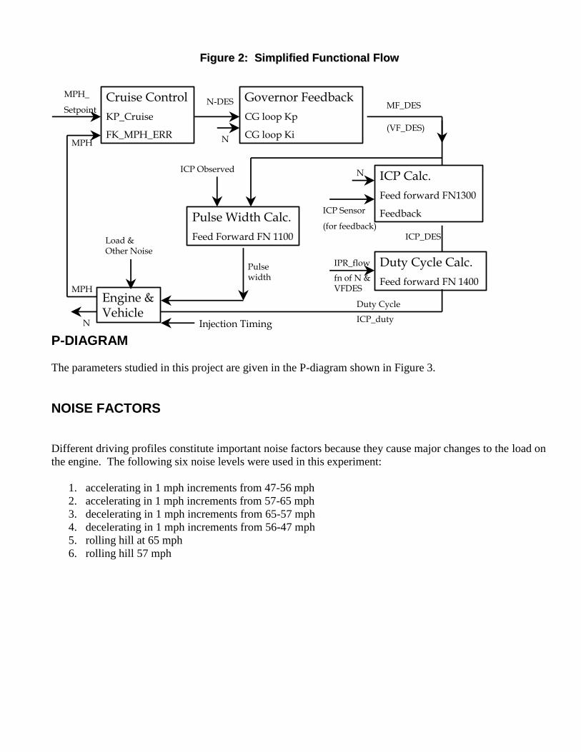
FFiigguurree 22:: SSiimmpplliiffiieedd FFuunnccttiioonnaall FFllooww
P-DIAGRAM
The parameters studied in this project are given in the P-diagram shown in Figure 3.
NOISE FACTORS
Different driving profiles constitute important noise factors because they cause major changes to the load on
the engine. The following six noise levels were used in this experiment:
1. accelerating in 1 mph increments from 47-56 mph
2. accelerating in 1 mph increments from 57-65 mph
3. decelerating in 1 mph increments from 65-57 mph
4. decelerating in 1 mph increments from 56-47 mph
5. rolling hill at 65 mph
6. rolling hill 57 mph
Cruise Control
KP_Cruise
FK_MPH_ERR
Engine & Vehicle
Duty Cycle Calc.
Feed forward FN 1400
Pulse Width Calc.
Feed Forward FN 1100
ICP Calc.
Feed forward FN1300
Feedback
Governor Feedback
CG loop Kp
CG loop KiN
N-DESMPH_
Setpoint
(VF_DES)
MF_DES
N
ICP Sensor
(for feedback)
fn of N & VFDES
IPR_flow
ICP_DES
Duty Cycle
ICP_dutyInjection TimingN
MPH
MPH
Load & Other Noise
ICP Observed
Pulse width
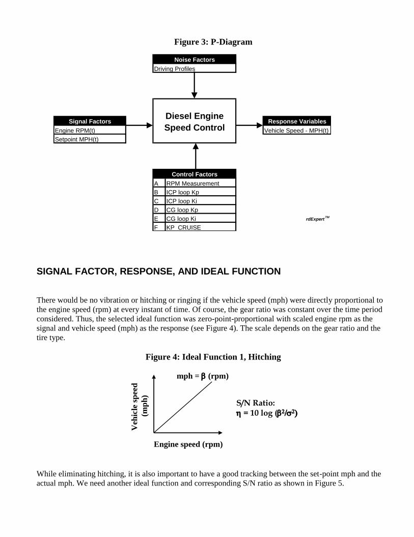
Figure 3: P-Diagram
SIGNAL FACTOR, RESPONSE, AND IDEAL FUNCTION
There would be no vibration or hitching or ringing if the vehicle speed (mph) were directly proportional to
the engine speed (rpm) at every instant of time. Of course, the gear ratio was constant over the time period
considered. Thus, the selected ideal function was zero-point-proportional with scaled engine rpm as the
signal and vehicle speed (mph) as the response (see Figure 4). The scale depends on the gear ratio and the
tire type.
Figure 4: Ideal Function 1, Hitching
While eliminating hitching, it is also important to have a good tracking between the set-point mph and the
actual mph. We need another ideal function and corresponding S/N ratio as shown in Figure 5.
mph = (rpm)
Engine speed (rpm)
Veh
icle
sp
eed
(mp
h)
S/N Ratio: = 10 log (
A RPM Measurement
B ICP loop Kp
C ICP loop Ki
D CG loop Kp
E CG loop Ki rdExpertTM
F KP_CRUISE
Signal Factors Response Variables
Control Factors
Noise Factors
Diesel Engine
Speed Control
Driving Profiles
Vehicle Speed - MPH(t)Engine RPM(t)
Setpoint MPH(t)

Figure 5: Ideal Function 2, Tracking
CONTROL FACTORS
Six control factors listed in Table 1 were selected for the study. These factors, various software speed
control strategy parameters, are described below:
Table 1: Control Factors and Levels
A) RPM Measurement is the number of consecutive measurements over which the rotational speed is
averaged for estimating rpm.
B) ICP loop Kp is the proportional constant for the ICP loop
C) ICP loop Ki is the integral constant for the ICP loop
D) CG loop Kp is the proportional constant for the Governor Feedback
E) CG loop Ki is the integral constant for the Governor Feedback
F) KP_CRUISE is the proportional constant for the Cruise Control feedback loop.
Label Factor Name No. of Levels
Level 1 Level 2 Level 3
A RPM Measurement 2 6 teeth 12 teeth
B ICP loop Kp 3 0.0005 0.0010 0.0015
C ICP loop Ki 3 0.0002 0.0007 00012
D CG loop Kp 3 0.8*(current) Current fn 1.2 (Current)
E CG loop Ki 3 0.027 0.032 0.037
F KP_CRUISE 3 0 0.5 (Current) Current
mph = (s_mph)
Setpoint speed (s_mph)
Veh
icle
sp
eed
(mp
h)
S/N Ratio: = 10 log (

EXPERIMENT PLAN AND DATA
An L18 orthogonal array was used for conducting the experiments. For each experiment, the vehicle was
driven under the six noise conditions. Data for rpm, mph set point, and actual mph were collected using
Tananko's vehicle instrumentation. About 1 minute's worth of data were collected for each noise condition.
Plots of scaled RPM (signal factor) versus actual mph (response) were used for calculation of the zero-
point-proportional dynamic S/N ratios. Plots for two experiments, showing low and high values for the S/N
ratio in the L18 experiment [corresponding to pronounced hitching (Expt 6) and minimal hitching (Expt 5)],
are shown in Figures 6a and 6b, respectively. The corresponding S/N ratios were: –1.8 and 11.8. This is an
empirical validation that the S/N ratio is capable of quantifying hitching.
Figure 6: Data Plots for Hitching Ideal Function
(a) (b)
FACTOR EFFECTS
Data from the L18 experiment were analyzed using rdExpertTM
software developed by Phadke Associates,
Inc. The control factor orthogonal array is given in the Appendix. The Signal/Noise (S/N) Ratio for each
factor level is shown in Figure 7. From the analysis shown in Figure 7, the most important factors are A, D,
and F.
Figure 7: Factor Effects for Ideal Function 1 (Hitching)
4 0
5 0
6 0
7 0
4 0 5 0 6 0 7 0
Re
sp
on
se
S i g n a l (E x p t. 6 )
4 0
5 0
6 0
7 0
4 0 5 0 6 0 7 0
Re
sp
on
se
S i g n a l (E x p t. 5 )

F Value 5.9 0.8 2.3 4.6 0.4 7.5
%SS 13.6 3.9 10.7 21.3 2.0 34.6
1) Factor A is the number of teeth in the flywheel associated with rpm calculations. The more teeth
used in the calculation, the longer the time associated with an rpm measurement and the greater the
smoothing of the rpm measure. Level 2, or more teeth, gives a higher S/N ratio, leading to reduced
hitching.
2) Factor D is CG loop Kp, a software constant associated with gain in the governor loop. Here Level
1, representing a decrease in the current function, is better.
3) Factor F is KP_Cruise, a software constant in the cruise control strategy associated with gain. Level
3, maintaining the current value for this function, is best, although Level 2 would also be acceptable.
Confirmation experiments using these factors were then conducted. Predicted values and observed values
were computed for the best levels of factors, the worst levels of factors, and the vehicle baseline (original)
levels of factors.
1) Best: A2, B3, C2, D1, E2, F3
2) Worst: A1, B1, C3, D3, E1, F1
3) Baseline: A1, B2, C1, D2, E2, F3
The results are shown in Table 2. We have shown the S/N ratios separately for noise conditions 1-4 and 5-6
to be able to ascertain that the hitching problem is resolved under the two very different driving conditions.
As can be seen in this table, there was very good agreement between the predicted and observed S/N ratios
under the above conditions.
Table 2: CCoonnffiirrmmaattiioonn EExxppeerriimmeenntt RReessuullttss
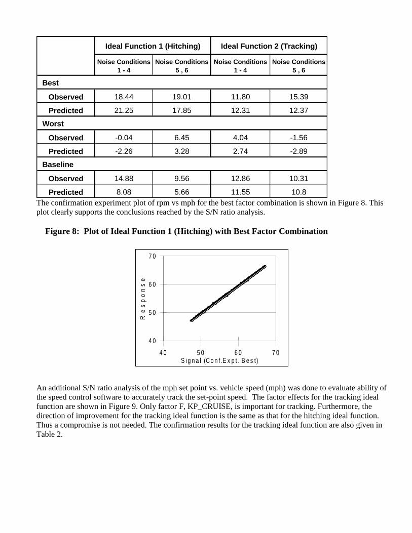
The confirmation experiment plot of rpm vs mph for the best factor combination is shown in Figure 8. This
plot clearly supports the conclusions reached by the S/N ratio analysis.
Figure 8: Plot of Ideal Function 1 (Hitching) with Best Factor Combination
An additional S/N ratio analysis of the mph set point vs. vehicle speed (mph) was done to evaluate ability of
the speed control software to accurately track the set-point speed. The factor effects for the tracking ideal
function are shown in Figure 9. Only factor F, KP_CRUISE, is important for tracking. Furthermore, the
direction of improvement for the tracking ideal function is the same as that for the hitching ideal function.
Thus a compromise is not needed. The confirmation results for the tracking ideal function are also given in
Table 2.
Noise Conditions
1 - 4
Noise Conditions
5 , 6
Noise Conditions
1 - 4
Noise Conditions
5 , 6
Observed 18.44 19.01 11.80 15.39
Predicted 21.25 17.85 12.31 12.37
Observed -0.04 6.45 4.04 -1.56
Predicted -2.26 3.28 2.74 -2.89
Observed 14.88 9.56 12.86 10.31
Predicted 8.08 5.66 11.55 10.8
Worst
Baseline
Ideal Function 1 (Hitching) Ideal Function 2 (Tracking)
Best
4 0
5 0
6 0
7 0
4 0 5 0 6 0 7 0
Re
sp
on
se
S i g n a l (C o n f.E x p t. B e s t)

Figure 9: Factor Effects for the Tracking Ideal Function
FURTHER IMPROVEMENTS
The factor effect plots of Figures 7 and 9 indicate that improvements beyond the confirmation experiment
can be achieved by exploring beyond Level A2 for Factor A, below Level D1 for Factor D, and beyond
Level F3 for Factor F. These extrapolations were subsequently tested and validated.
CONCLUSIONS
The team now knew how to completely eliminate hitching. Many members of this team had been working
on this problem for quite some time. They believed it to be a very difficult problem that most likely would
never be solved. The results of this study surprised some team members and made them believers in the
Robust Design approach. In the words of one of the team members, "When we ran that confirmation
experiment and there was no hitching, my jaw just dropped. I couldn't believe it. I thought for sure this
would not work. But now I am telling all my friends about it and I intend to use this approach again in
future situations."
After conducting only one L18 experiment, the team gained tremendous insights into the hitching
phenomenon and how to avoid it. They understood on a root-cause level what was happening, made
adjustments, and conducted a complete prove-out program that eliminated hitching without causing other
undesirable vehicle side effects. As a result of this effort, a 12 R/1000 reliability problem with associated
warranty costs of over eight million dollars, was eliminated.
F Value 4.2 0.1 0.2 1.6 0.1 118.3
% SOS 1.7 0.0 0.2 1.3 0.1 94.4

ACKNOWLEDGEMENTS
The following persons contributed to the success of this project:
Ford Motor Company: Ellen Barnes, Harish Chawla, David Currie, Leighton Davis Jr.,
Donald Ignasiak, Tracie Johnson, Arnold Kromberg,
Chris Kwasniewicz, Bob McCliment, Carl Swanson,
Dmitry Tananko, Laura Terzes, Luong-Dave Tieu
International Truck Co.: Dan Henriksen, William C Rudhman
Visteon Corporation: David Bowden, Don Henderson
The authors especially thank Dr. Carol Vale of the Ford Motor Company for her valuable comments in
editing this manuscript.
REFERENCES
Proseanic, V., Tananko, D., Visnepolschi, S. "The Experience of the Anticipatory Failure Determination
(AFD) Method Applied to Hitching/Ringing Problems." TRIZCON2000, The Second Annual Altshuller
Institute TRIZ Conference Proceedings, Nashua, NH, 2000, pp. 119-126.
Phadke, M.S. Quality Engineering Using Robust Design, Prentice Hall, Englewood Cliffs, NJ, November
1989.
Taguchi, Genichi System of Experimental Design, Edited by Don Clausing, New York: UNIPUB/Krass
International Publications, Volume 1 & 2, 1987.
The data were analyzed by using the rdExpert software developed by Phadke Associates, Inc. rdExpert is a
trademark of Phadke Associates, Inc.

APPENDIX
Control Factor Orthogonal Array (L18)
Expt
No.
A : Col. 1
RPM
Measurement
B : Col. 2
ICP loop Kp
C : Col. 3
ICP loop Ki
D : Col. 4
CG loop Kp
E : Col. 5
CG loop Ki
F : Col. 6
KP_CRUISE
1 1) 6 teeth 1) 0.0005 1) 0.0002 1) 0.8*(current) 1) 0.027 1) 0
2 1) 6 teeth 1) 0.0005 2) 0.0007 2) Current fn 2) 0.032 2) 0.5 (Current)
3 1) 6 teeth 1) 0.0005 3) 00012 3) 1.2 ( Current) 3) 0.037 3) Current
4 1) 6 teeth 2) 0.0010 1) 0.0002 1) 0.8*(current) 2) 0.032 2) 0.5 (Current)
5 1) 6 teeth 2) 0.0010 2) 0.0007 2) Current fn 3) 0.037 3) Current
6 1) 6 teeth 2) 0.0010 3) 00012 3) 1.2 ( Current) 1) 0.027 1) 0
7 1) 6 teeth 3) 0.0015 1) 0.0002 2) Current fn 1) 0.027 3) Current
8 1) 6 teeth 3) 0.0015 2) 0.0007 3) 1.2 ( Current) 2) 0.032 1) 0
9 1) 6 teeth 3) 0.0015 3) 00012 1) 0.8*(current) 3) 0.037 2) 0.5 (Current)
10 2) 12 teeth 1) 0.0005 1) 0.0002 3) 1.2 ( Current) 3) 0.037 2) 0.5 (Current)
11 2) 12 teeth 1) 0.0005 2) 0.0007 1) 0.8*(current) 1) 0.027 3) Current
12 2) 12 teeth 1) 0.0005 3) 00012 2) Current fn 2) 0.032 1) 0
13 2) 12 teeth 2) 0.0010 1) 0.0002 2) Current fn 3) 0.037 1) 0
14 2) 12 teeth 2) 0.0010 2) 0.0007 3) 1.2 ( Current) 1) 0.027 2) 0.5 (Current)
15 2) 12 teeth 2) 0.0010 3) 00012 1) 0.8*(current) 2) 0.032 3) Current
16 2) 12 teeth 3) 0.0015 1) 0.0002 3) 1.2 ( Current) 2) 0.032 3) Current
17 2) 12 teeth 3) 0.0015 2) 0.0007 1) 0.8*(current) 3) 0.037 1) 0
18 2) 12 teeth 3) 0.0015 3) 00012 2) Current fn 1) 0.027 2) 0.5 (Current)

S/N Ratios
Noise 1-4 Noise 5-6 Noise 1-4 Noise 5-6
1 2.035 9.821 3.631 -2.996
2 11.078 4.569 11.091 7.800
3 4.188 4.126 9.332 9.701
4 15.077 7.766 11.545 8.256
5 11.799 3.908 12.429 9.233
6 -1.793 3.001 3.415 -1.390
7 9.798 4.484 11.841 9.793
8 5.309 6.212 4.392 -2.053
9 8.987 8.640 9.618 9.324
10 13.763 12.885 10.569 10.267
11 18.550 18.680 12.036 14.106
12 2.538 15.337 1.826 -3.128
13 0.929 16.065 1.492 -1.200
14 9.022 9.501 8.688 7.856
15 18.171 18.008 11.260 14.804
16 11.734 11.823 12.031 11.852
17 18.394 16.338 7.000 -1.881
18 13.774 17.485 9.943 9.142
Average 9.631 10.480 8.452 6.083
Exp No.Hitching S/N Tracking S/N


