

Technical Report Documentation Page
L Report No.
TX-9511994-5 I 2. Government AccesSIOn No. 3. Recipient's Catalog No.
4. Title and Subtitle
REDUCTION OF SULFATE SWELL IN EXPANSIVE CLAY SUBGRADES IN THE DALLAS DISTRICT
5. Report Date
November 1994 Revised: May 1995
7. Author(s)
Sanet Bredenkamp and Robert L. Lytton 9. Performmg Organizatton Name and Address
Texas Transportation Institute The Texas A&M University System College Station, Texas 77843-3135 12. Sponsoring Agency Name and Address
Texas Department of Transportation Research and Technology Transfer Office P. O. Box 5080 Austin, Texas 78763-5080
1:>. ::.upplementary Notes
6. Performing UIganization Code
IS.Pertomung orgaruzaaon Keport No.
Research Report 1994-5 10. Work Urut No. (TRAIS)
1 L Contract or (jrant No.
Study No. 7-1994, Task 16 13. Type of Report and Period Covered
Interim: September 1993 - August 1994 14. sponsoring Agency Code
Research performed in cooperation with the Texas Department of Transportation. Research Study Title: Highway Planning and Operation for District 18 Phase III 16. Abstract
The addition of hydrated lime to clay soils is one of the most common methods of soil stabilization. However, when sulfates are present in the soil, the calcium in the lime reacts with the sulfates to form ettringite, an expandable mineral. This expansion causes a considerable amount of economical as well as structural problems. Sulfate related heave has been experienced along IH 45 and FM 1382. In this research, a field test method was developed to locate sulfate bearing soils. A permittivity probe was used to measure the electrical conductivity of the in situ soil. The electrical conductivity was then related to sulfate content in soils. Expansion tests were performed to determine the amount of expansion that occurs when lime is added to soils with different sulfate contents. A model that relates the amount of expansion of clay soils to electrical conductivity was proposed. The use of low calcium fly-ashes were investigated and proposed as an alternative form of stabilizer for sulfate bearing soils.
17. Key Words 1 IS. DlStnbutton Statement
Sulfate Swell, Ettringites, Low Calcium Fly-Ash Stabilizers
No restrictions. This document the public through NTIS:
19. Security Classif.(of this report)
Unclassified Form DOT F 1700.7 (8-72)
National Technical Information 5285 Port Royal Road Springfield, Virginia 22161
1
20. Security Classif.(ot ms page) 21. No. of Pages
Unclassified 124 ReproductioD of completed page authonzed
is available to
Service

REDUCTION OF SULFATE SWELL IN EXPANSIVE CLAYSUBGRADES IN THE DALLAS DISTRICT
by
Sanet Bredenkamp Research Assistant
Texas Transportation Institute
and
Robert L. Lytton Research Engineer
Texas Transportation Institute
Research Report 1994-5 Research Study Number 7-1994, Task 16
Research Study Title: Highway Planning and Operation for District 18 Phase III
Sponsored by the Texas Department of Transportation
November 1994 Revised: May 1995
TEXAS TRANSPORTATION INSTITUTE The Texas A&M University System College Station, Texas 77843-3135


IMPLE:MENT ATION STA TE:MENT
Sulfate related heave was experienced along FM 1382 and rn: 45. The
mechanism of the heave and a proposed solution to the problem are described in
this report. A field measurement procedure to determine an estimated amount of
sulfate related heave before and after lime stabilization is described. Electrical
conductivity is related to sulfate content and can, therefore, be used to determine
whether substantial amounts of sulfates are present and whether they will cause a
problem upon lime stabilization. Three different low calcium fly-ashes were used as
alternative stabilization methods for sulfate bearing soils. The fly-ashes performed
well and their results are described in this report.
The field measurement procedure developed in this project is sufficiently
promising to warrant pilot and subsequently full implementation by those district
laboratories which must contend with sulfate swelling subgrades. A step-by-step
procedure to determine sulfate related expansion in clay soils is included in the
implementation section at the end of this report.
v


DISCLAIMER
The contents of this report reflect the views of the authors who are
responsible for the facts and accuracy of the data presented herein. The contents
do not necessarily reflect the official views or policies of the Texas Department of
Transportation. This report does not constitute a standard, specification, or
regulation.
vii

TABLE OF CONTENTS
Page
LIST OF FIGURES ..... ',' ...................................... xiii
LIST OF TABLES .............................................. xvi
SUMMARY .................................................. xix
CHAPTER 1 INTRODUCTION . . . . . . . . . . . . . . . . . . . . . . . . . . . . . . . . . .. 1
CHAPTER 2 liTERATURE REVIEW .............................. 5
Introduction ............................................... 5
Conductivity of Soils ......................................... 5
Electrical Conductivity in Soils ............................. 5
Conventional Methods for Measuring Soil
Electrical Conductivity ................................... 6
Relation of Conductivity to Salt Content
and Osmotic Pressure .................................... 8
The Effect of Soil: Water Ratios on the
,Electrical Conductivity ................................... 8
The Effect of Temperature on Conductivity ........ . . . . . . . . . . .. 8
Electrical Conductivity Measurements with
Permittivity Probe ...................................... 13
Mineralogy of Clay Soils ..................................... 13
Stabilization of Base Courses with Lime . . . . . . . . . . . . . . . . . . . . . . . . .. 18
Formation of Ettringites ..................................... 18
CHAPTER 3 METHODOLOGY .................................. 21
Introduction .............................................. 21
Method for Determination of Expansion of
Sulfate Bearing Clay Soils .................................... 22
Method for Determining Electrical Conductivity
with Permittivity Probe and the EPA Method
No. 9050 ................................................. 25
ix

Page
Method for Investigating Several Low Calcium Fly-Ashes
as Alternative Stabilizers ..................................... 28
Methods by which Supplementary Tests were
Performed ................................................ 28
Cation Exchange Capacity Determination .................... 28
Method for Determination of Soluble Sulfate Content ........... 29
Method for Determination of Dielectric Constants ............. 29
CHAPTER 4 RESULTS FROM EXPANSION TESTS ................ ,. 31
Introduction .............................................. 31
Results of Expansion Tests Performed on
Samples from IH 45 and FM 1382 . . . . . . . . . . . . . . . . . . . . . . . . . . . . .. 31
Results of Expansion Tests Performed on
Clay Soil Samples .......................................... 39
Conclusions ............................................... 42
CHAPTER 5 RESULTS FROM ELECTRICAL CONDUCTIVITY
MEASUREMENTS ............................................. 43
Introduction .............................................. 43
Results from Soluble Sulfate Determination ....................... 43
Results from Electrical Conductivity Measurements on
Soil Samples Obtained from IH 45 and FM 1382 . . . . . . . . . . . . . . . . . .. 45
Results from Electrical Conductivity
Measurements on Four Clay Soils .............................. 45
Water Content of the In Situ Soil .............................. 54
Conclusions ............................................... 55
CHAPTER 6 RESULTS OF SUPPLEMENTARY TESTS ............... 57
Introduction .............................................. 57
Results from Cation Exchange Capacity Determination .............. 57
Results of Dielectric Constant Measurements ...................... 59
Conclusions ............................................... 63
x
Page
CHAPTER 7 RESULTS OF LOW CALCIUM FLY-ASH
STABILIZATION .............................................. 65
Introduction .............................................. 65
Results of Low Calcium Fly-Ash Stabilization
on Four Clay Soils . . . . . . . . . . . . . . . . . . . . . . . . . . . . . . . . . . . . . . . . .. 65
Results of Low Calcium Fly-Ash Stabilization on
FM 1382 Site No 7 ......................................... 69
Evaluation of Different Low Calcium
Fly-Ashes as Stabilizers ...................................... 70
Conclusions ............................................... 71
CHAPTER 8 INTERACTIVE DISCUSSION OF ALL RESULTS ......... 73
Introduction .............................................. 73
Modell: Regression Modeling with % Expansion without Lime
as Response Variable for the Four Clay Soil Samples ............... 73
Model 2: Regression Modeling with % Expansion with 6% Lime
as Response Variable for the Four Clay Soil Samples ............... 76
Model 3: Regression Modeling with % Expansion without Lime
as Response Variable for Soil Samples from FM 1382 and IH 45 ....... 77
Model 4: Regression Modeling with % Expansion with 6% Lime
as Response Variable for Soil Samples from FM 1382 and IH 45 ....... 79
Model for Determination of Amount of Expansion Experienced
by Sulfate Bearing Clay Soils ................................ " 81
Conclusions ............................................... 82
CHAPTER 9 CONCLUSION ..................................... 85
Overall Conclusions ......................................... 85
Subjects Proposed for Further Investigation ....................... 86
CHAPTER 10 IMPLEMENTATION OF RESULTS .................... 89
REFERENCES ................................................ 93
xi

Page
APPENDIX A . . . . . . . . . . . . . . . . . . . . . . . . . . . . . . . . . . . . . . . . . . . . . . . .. 97
Locations from which Soil Samples Were Taken Along FM 1382 ....... 99
Locations from which Soil Samples Were Taken Along IH 45 ......... 100
APPENDIX B ................................................. 101
Relation Between PH of Clay Soils and Amount of Expansion
Encountered .............................................. 103
xii

LIST OF FIGURES
Page
1 Schematic Outline of Testing and Reporting Procedure ............... 4
2 Wenner Array of Electrodes Used in Soil Electrical Conductivity
Determinations (5) .......................................... 7
3 Volume of Soil Measured Using Wenner Array Method (5) ............ 7
4 Concentration of Single-Salt Solutions in Milliequivalents per Liter as
Related to Electrical Conductivity (4) . . . . . . . . . . . . . . . . . . . . . . . . . . . .. 9
5 Concentration of Single-Salt Solutions in Percent as Related to Electrical
Conductivity (4) .... . . . . . . . . . . . . . . . . . . . . . . . . . . . . . . . . . . . . . . .. 10
6 Osmotic Pressure of Saturation Extracts of Soils as Related to Electrical
Conductivity (4) ............... . . . . . . . . . . . . . . . . . . . . . . . . . . . .. 11
7 Layer Structure of a 2:1 Clay Mineral (Smectite) (10) . . . . . . . . . . . . . . .. 15
8 Layer Structure of Mica Mineral (10) . . . . . . . . . . . . . . . . . . . . . . . . . . .. 16
9 Layer Structure of 1:1 Clay Mineral (Kaolinite) (10) . . . . . . . . . . . . . . . . 16
10 Arrangement of H20 Chains Linking a Divalent Exchange Cation on the
Surfaces of a) a 1.5 nm Hydrate of Vermiculite and b) a 2 nm Hydrate
of Smectite (10) . . . . . . . . . . . . . . . . . . . . . . . . . . . . . . . . . . . . . . . . . . .. 17
11a Expansion of Soil Samples from FM 1382 Containing 6% Lime ........ 32
11b Expansion of Soil Samples from FM 1382 Containing No Lime ........ 32
12a Expansion of Soil Samples from IH 45 Containing 6% Lime. . . . . . . . . .. 33
12b Expansion of Soil Samples from IH 45 Containing No Lime ........... 33
13a Expansion of Soil Samples Containing 6% Lime vs. Sulfate Content 34
13b Expansion of Soil Samples Containing No Lime vs. Sulfate Content 34
14 Expansion of Samples Containing No Lime. Sample on Left Contains
Less than 0.2% Sulfates and Sample on Right 0.8% Sulfates. .......... 36
xiii
Page
15 Samples Containing 6% Lime. The Two Samples on the Left Contain
0.8% Sulfates and Expanded 18%. The Sample on the Right Contains
Less than 0.2% Sulfates and is Still Close to Original Size ............ 37
16 Two Soil Samples with 0.8% Sulfates. Sample on the Left Contains 6%
Lime and Expanded 6% More than the Sample on the Right Which
Contains No Lime .......................................... 38
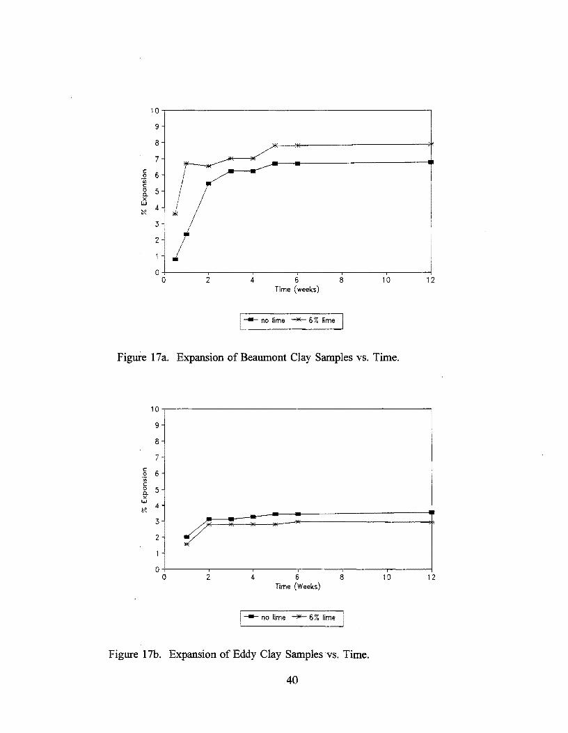
17a Expansion of Beaumont Clay Samples vs. Time .................... 40
17b Expansion of Eddy Clay Samples vs. Time ........................ 40
17c Expansion of Houston Black Clay Samples vs. Time ................. 41
17d Expansion of Kaolinitic Samples ............................... 41
18 Relation Between Electrical Conductivity and Natural Sulfate Content of
Soil Samples from FM 1382 and IH 45 . . . . . . . . . . . . . . . . . . . . . . . . . .. 46
19 Regression Line for Electrical Conductivity and Sulfate Content ........ 46
20a Electrical Conductivity vs. Sulfate Content of a Beaumont Clay ........ 47
20b Electrical Conductivity vs. Sulfate Content of an Eddy Clay .. .. .. .. .. .. .. .. .. .. .. 47
20c Electrical Conductivity vs. Sulfate Content of a Houston Black Clay ..... 48
20d Electrical Conductivity vs. Sulfate Content of Kaolinite ............... 48
20e Electrical Conductivity vs. Chloride and Sulfate Content ,. .. .. .. .. .. .. .. .. .. .. .. .. . 50
21 Electrical Conductivity Values of the Four Clay
Soils vs. Sulfate Content ...................................... 51
22 Regression Line Fitted through Mean Values of Electrical Conductivity
for Different Sulfate Contents ................................. 51
23a Dielectric Constant vs. Frequency for an Eddy Clay. . . . . . . . . . . . . . . .. 60
23b Dielectric Constant
23c Dielectric Constant
23d Dielectric Constant
vs. Frequency for a Beaumont Clay .. .. . . .. .. .. .. ~ .. .. .. .. ..
vs. Frequency for a Houston Black Clay ...........
vs. Frequency for a Kaolinitic Clay ...............
60
61
61
24 Relation Between the Dielectric Constant and the Amount of Added
Sulfates .................................................. 62
25 Relation Between the CEC and the Range of Eo-Values .............. 64
xiv

Page
26 Relation Between CEC and Range of a-Values .................... 64
27a Expansion of an Eddy Clay Upon Stabilization with Various Low
Calcium Fly-Ashes ... . . . . . . . . . . . . . . . . . . . . . . . . . . . . . . . . . . . . . .. 66
27b Expansion of a Beaumont Clay Upon Stabilization with Various Low
Calcium Fly-Ashes .......................................... 67
27c Expansion of a Houston Black Clay Upon Stabilization with Various Low
Calcium Fly-Ashes .. . . . . . . . . . . . . . . . . . . . . . . . . . . . . . . . . . . . . . . .. 68
27d Expansion of a Kaolinitic Clay Upon Stabilization with Various Low
Calcium Fly-Ashes .......................................... 68
28 Expansion of Eddy Clay from FM 1382 Site No.7 Upon Stabilization
with Montecello Low Calcium Fly-Ash. . . . . . . . . . . . . . . . . . . . . . . . . .. 69
29 The Average Amount of Expansion for Each Stabilizer vs. the Calcium
Content of the Stabilizer ..................................... 70
30 Battery Driven Digital Scale . . . . . . . . . . . . . . . . . . . . . . . . . . . . . . . . . .. 90
31 Hand Held Electrical Conductivity Meter ......................... 90
32 Relation Between pH of Clay Soils and the Amount of Expansion After
Lime Stabilization .......................................... 103
xv

LIST OF TABLES
Page
1 Bureau of Soils Data for Reducing Soil Paste Resistance Readings to
Values at 15.5°C (60 °F)(4) .................................. 12
2 Ratios of Lime and Sulfates Added to the Four Clay Soil Samples 23
3a Composition of Soil Samples on which Electrical Conductivity
Measurements were Performed (Samples Containing Natural Soil and
Sulfates) ................................................. 26
3b Composition of Soil Samples on which Electrical Conductivity
Measurements were Performed (Samples Containing Natural Soil,
Sulfates and Chlorides) ...................................... 26
3c Composition of Soil Samples on which Electrical Conductivity
Measurements were Performed (Samples Containing Natural Soil,
Sulfates and Lime) ... . . . . . . . . . . . . . . . . . . . . . . . . . . . . . . . . . . . . . .. 27
4a Amount of Soluble Sulfates in the Four Clay Soil Samples ............ 44
4b Amount of Soluble Sulfates in the Soil Samples Obtained from FM 1382
and IH 45 ................................................ 44
5 Mean· Electrical Conductivity Value at Different Sulfate Contents, with
Standard Deviation ......................................... 52
6 Comparison between Electrical Conductivity Measurements of Single-Salt
Solution and Soil Solutions at the Same Sulfate Concentration ......... 53
7a Cation Exchange Capacities for the Four Clay Soil Samples ........... 58
7b Cation Exchange Capacities for Soil from FM 1382 and IH 45 ......... 58
8 Values for a Calculated from Known Values of e at Different
Frequencies with Values for CEC .............................. 62
9 Results of Various Experimental Procedures for the Four Clay Soil
Samples (Without Lime) ..................................... 74
xvi

Page
10 Pearson Correlation Coefficients for Expansion of Clay Soil Samples
Containing No Lime, and Other Parameters (19) ................... 75
11 Results of Various Experimental Procedures for the Four Clay Soil
Samples (With Lime) ........................................ 76
12 Pearson Correlation Coefficients for Expansion of Clay Soil Samples
Containing 6% Lime, and Other Parameters (19) ................... 76
13 Results of Various Experimental Procedures for Soil Samples from FM
1382 and IH 45 (Without Lime) ................................ 78
14 Pearson Correlation Coefficients for Expansion of Soil Samples from FM
1382 and IH 45 Containing No Lime, and Other Parameters (19) ....... 78
15 Results of Various Experimental Procedures for Soil Samples from FM
1382 and IH 45 (With Lime) .................................. 80
16 Pearson Correlation Coefficients for Expansion of Soil Samples from FM
1382 and IH 45 Containing 6% Lime, and Other Parameters (19) . . . . . .. 80
xvii


SUMMARY
Hydrated lime is in many cases added to clay soils to reduce the amount of
expansion. The lime-soil-water system creates a high pH environment which
enhances flocculation. However, when sulfates are present in the soil, the lime
reacts with the sulfates to form ettringites, an expandable mineral. Ettringites can
expand up to 200% of their original size. The formation of ettringite causes great
economical as well as structural problems.
This report describes a method that can be used to determine the sulfate
content of in situ soil. The sulfate content of soil is related to electrical conductivity
measured on a soil paste with a specific soil-water ratio. The sulfate content is also
related to the amount of expansion that occurs upon lime stabilization. The report
proposes equations that give an approximate amount of expansion due to sulfates in
the soil as a function of the sulfate content and the electrical conductivity. The
approximate amount of expansion before and after lime stabilization can be
obtained by using the relationship between expansion, electrical conductivity, and
sulfate content. The only parameter needed to determine an approximate amount of
expansion is the electrical conductivity. Electrical conductivity can be measured with
great ease on a soil paste. This measurement can be made in the field, and does not
require expensive laboratory equipment.
The report also discusses alternative methods to stabilize sulfate bearing clay
soils. Low calcium fly-ash stabilizers are proposed for stabilizing sulfate bearing clay
soils. The low calcium stabilizers proposed are Montecello, Big Brown, and Sandow
fly-ashes. These fly-ashes performed well in keeping some sulfate bearing clay soils
from expanding.
xix

CHAPTERl
INTRODUCTION
Lime is an inexpensive and available mineral which, when added to clay soils,
raises the pH of the soil, adds stability, and increases strength. Lime is used to
stabilize clay soils in various applications, of which the road industry is one primary
example.
However, when using lime to stabilize some sulfate bearing soils, excessive
heave which is detrimental to roadways and other constructions is induced.
Research indicates that this heave may be due to the reaction between calcium in
the lime and naturally occurring sulfates in the soil which leads to the formation of
the expandable minerals ettringite and thaumasite (1). Alternative methods for
stabilizing sulfate bearing soils have been investigated. For example, Ferris et al.
recommended the use of barium compounds as alternative stabilizing agents when
stabilizing sulfate bearing soils (2).
Before such alternative methods can be employed, however, sulfate bearing
soils need to be identified. An easy-to-perform field test is needed to determine
whether sulfates are present in soil.
The electrical conductivity of the soil is a relatively easily measured parameter
that relates to the sulfate content of soil (3). A high electrical conductivity could
indicate the presence of sulfates, and electrical conductivity measurement can be
used to locate possible problem sites. The mineralogy of the clay may have an
effect on the formation of ettringite. In this thesis, four different clay soils will be
subjected to expansion tests after the addition of lime and sulfates, to investigate the
relative volume changes of the four standard soil samples at different sulfate
contents.
The specific objectives of this study are summarized below:
1) To identify the cause of heave of those clay soils that expanded after
lime stabilization.
1

2) To establish a field test that can locate soils containing sulfates. The
hypothesis states that the electrical conductivity of soil has a strong
relation to the sulfate content in the soil, and since electrical
conductivity is easily measurable, it could be established as a field test
for the determination of possible sulfate induced heave in clay soils.
3) To investigate the possible relationship between the cation exchange
capacity (CEC) of the clay and the amount of heave that occurs when
sulfate bearing soils are stabilized with lime. (CEC is an inherent soil
property that relates to the mineralogy of different clay soils and to their
specific surface area.)
4) To determine the minimum amount of sulfates that cause the formation
of expandable ettringite.
5) To attempt to identify an alternative stabilizing agent to stabilize sulfate
bearing soils.
A discussion of the two major types of experiments performed follows. The
first experiment tests swelling to determine the expansion of soil samples containing
natural sulfates and lime as well as added sulfates and lime. It will also determine
the expansion of soil samples which were stabilized with low calcium fly-ash like:
Sandow, Big Brown, and Montecello. The second set of experiments were
performed to determine the presence of sulfates in the soil samples. The amount of
sulfates was determined by two different electrical conductivity methods, the first
being the standard EPA procedure and the second using a permittivity probe which
measures both electrical conductivity and the dielectric constant of the soil. As a
control measure, the amount of sulfates was also determined with an EPA
procedure for the determination of total sulfate content.
Other experiments performed were the CEC determination and the dielectric
constant (DC) determination. These experiments were performed in order to gain a
better understanding of the properties of clay which could have an influence on
expansive behavior. The results and conclusions of each of the above mentioned
2

experiments are presented in the chapters following the description of the methods
used to perform the experiments.
Finally, a conclusion is made which describes how the results of the different
experiments interact with each other. The conclusion states how electrical
conductivity could be used to determine locations of sulfate bearing soils and makes
suggestions about alternative procedures by which sulfate bearing soils could be
stabilized. The following flow chart describes the layout of this study schematically.
3

"Tj ......
~ .......
r:F.l (") g-:3 ~ ...... (")
0 a ...... ~ 0 H')
>-l ('j)
.J:..
til g. (IQ
8-~ -g g.
(IQ
with lime
~ a (") ('j) (:l..
~ l Conclusionmj
PROBLEM: Sulfate swelling upon lime stabilization
Experimental methods
Interactive conclusions
Sulfate etermination Supplementary tests
I E.C. d~l~~~inatiOI~ permittivity probe
Results
I
L ··1
Sulfate determination by EPA method
l~thersaltsl
DC Determination

CHAPfER2
LITERATURE REVIEW
INTRODUCTION
The general idea of this study is that electrical conductivity of soils can be
related to the sulfate content in the soil. An attempt will also be made to suggest
alternative stabilization methods for sulfate bearing soils.
In order to develop a relationship between electrical conductivity and sulfate
content, it is necessary to have an understanding of the basic electrical properties
associated with soils as well as an understanding of the mineralogy of the different
soils under investigation. This chapter will discuss the electrical properties of soil as
well as the . basic mineralogy of the soils under investigation.
This chapter also provides an overview of the chemistry involved in the
formation of ettringites, which is an expandable mineral formed when sulfate
bearing soils are stabilized with lime. State-of-the-art stabilization methods are also
discussed in this chapter.
CONDUCTnnTYOFSOn£
Electrical Conductivity in Soils
Electrical conductivity is defmed as the reciprocal of the electrical resistivity
(4). Resistivity is the resistance (in ohms) of a metallic or electrolytic conductor,
which is 1 cm long and has a cross sectional area of 1 cm2• Hence, electrical
conductivity is expressed in reciprocal ohms per centimeter, or Siemens (mhos) per
centimeter (4).
Soil minerals are insulators, and electrical conductivity of soil is primarily
facilitated through pore water which contains electrolytes (5). Exchangeable cations
contribute little to the electrical conductivity of soils because of the abundance and
increased mobility of the soluble electrolytes (5). Electrical conductivity is
influenced by the amount and size of the water pores in soil, as well as the water
content and the concentration of electrolytes in the soil (5). The salt content of a
5
saturated soil paste can be estimated by using electrical conductivity measurements
(4). A more accurate estimate can be obtained by electrical conductivity
measurements of the water extracted from the soil (5).
Conventional Methods for Measuring Soil Electrical Conductivity
Soil salinity or soil electrical conductivity measurements can be detennined
from measurements of bulk electrical conductivity using the four electrode method
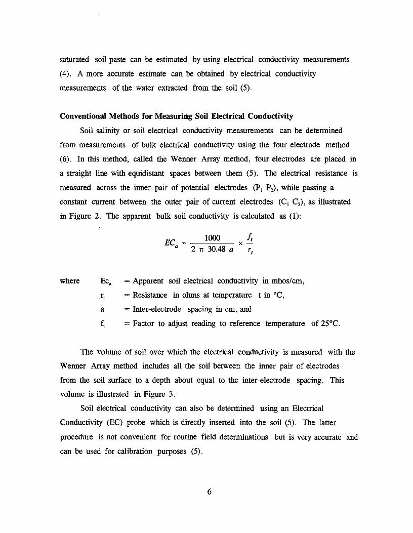
(6). In this method, called the Wenner Array method, four electrodes are placed in
a straight line with equidistant spaces between them (5). The electrical resistance is
measured across the inner pair of potential electrodes (PI P2), while passing a
constant current between the outer pair of current electrodes (C] C2), as illustrated
in Figure 2. The apparent bulk soil conductivity is calculated as (1):
where
1000 ECa - -----
2 1t 30.48 a
Eca = Apparent soil electrical conductivity in mhos/cm,
f t = Resistance in ohms at temperature t in °C,
a = Inter-electrode spacing in cm, and
ft = Factor to adjust reading to reference temperature of 25°C.
The volume of soil over which the electrical conductivity is measured with the
Wenner Array method includes all the soil between the inner pair of electrodes
from the soil surface to a depth about equal to the inter-electrode spacing. This
volume is illustrated in Figure 3.
Soil electrical conductivity can also be detennined using an Electrical
Conductivity (EC) probe which is directly inserted into the soil (5). The latter
procedure is not convenient for routine field detenninations but is very accurate and
can be used for calibration purposes (5).
6
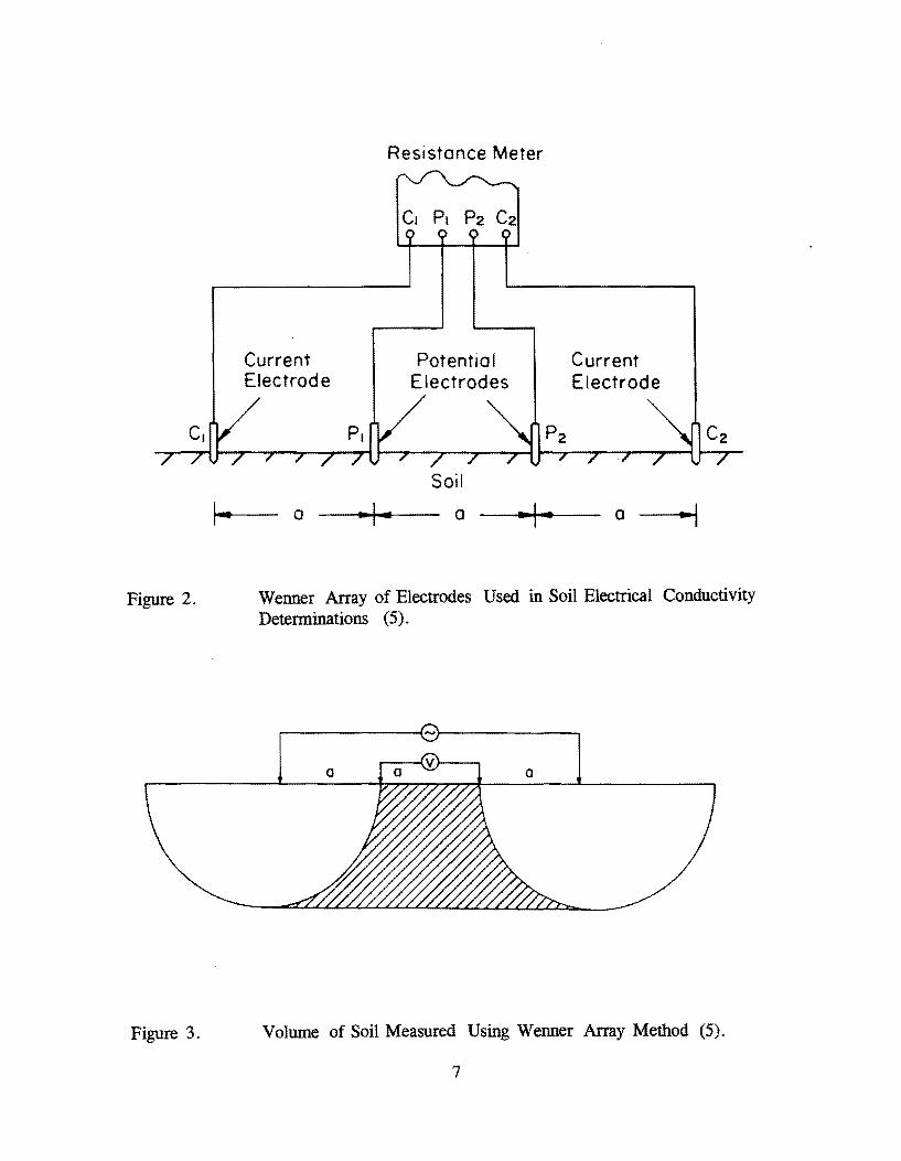
Figure 2.
Figure 3.
Current Electrode
a
Resistance Meter
Potential Electrodes
Soil
a "I-
Current Electrode
a
Wenner Array of Electrodes Used in Soil Electrical Conductivity Detenninations (5).
Volume of Soil Measured Using Wenner Array Method (5).
7

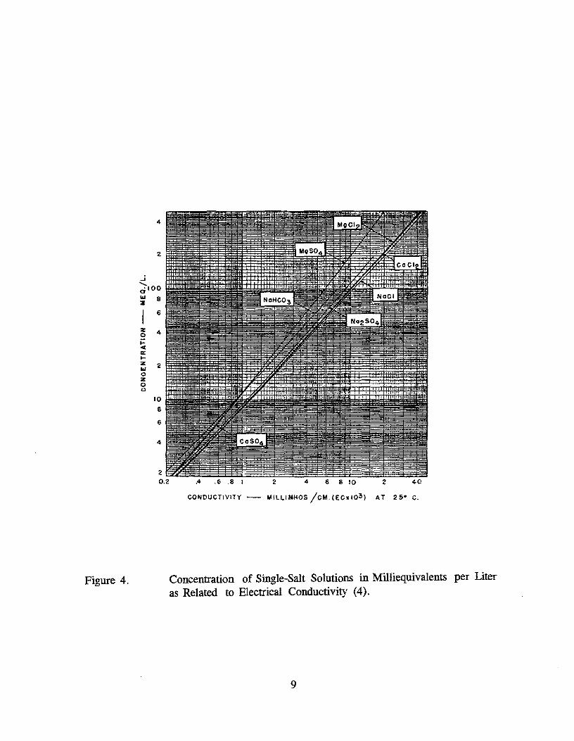
Relation of Conductivity to Salt Content and Osmotic Pressure
The relationships between electrical conductivity and salt content of different
solutions are shown graphically in Figures 4 and 5 (4). The curves for Na2S04 and
the chloride salts almost coincide. but MgS04 • CaS04 • and NaHC03 have lower
conductivities than the other salts at equivalent concentrations. When the
concentration is given as percent salt, the curves are more widely spread (4).
Experimental work done by salinity laboratories indicates a strong relationship
between the electrical conductivity and osmotic pressure of a solution. Figure 6
shows this relationship (4). In the range of electrical conductivity that will permit
plant growth, the osmotic pressure is given by:
OP - 0.36 x EC x loJ
where OP = Osmotic pressure.
Since the electrical conductivity of the soil is related to osmotic pressure, the latter
could also be used to determine the salt content in soils.
The Effect of Soil:Water Ratios on the Electrical Conductivity
When the extract is obtained from solutions with soil:water ratios of 1: 1 and
1 :5, conductivity measurements are used for estimating salinity (4). For a chloride
salt, the electrical conductivity results will only be slightly influenced by the water
content, but with low soluble salts like sulfates and carbonates, the apparent amount
of salt will be dependent on the soil:water ratio. For this reason it is necessary to
report electrical conductivity measurements at specific soil:water ratios (4).
The Effect of Temperature on Conductivity
The electrical conductivity of soil increases approximately 2 % with each
degree centigrade increase in temperature (4). The resistance of 9 soils at 13
temperatures was measured and the average relation of resistance to temperature
calculated (4). This relationship is given in Table 1.
8
4
2
...i ~IOO 0 III 8 :IE
6
z 4 0 i= « a:: ... z 2 III 0 Z 0 0
10
8
6
4
Figure 4.
2 4 6 8 10 2 40
CONDUCTIVITY - MILLIMHOS /CM.(ECxI03 ) AT 25- C.
Concentration of Single-Salt Solutions in Milliequivalents per Liter as Related to Electrical Conductivity (4).
9
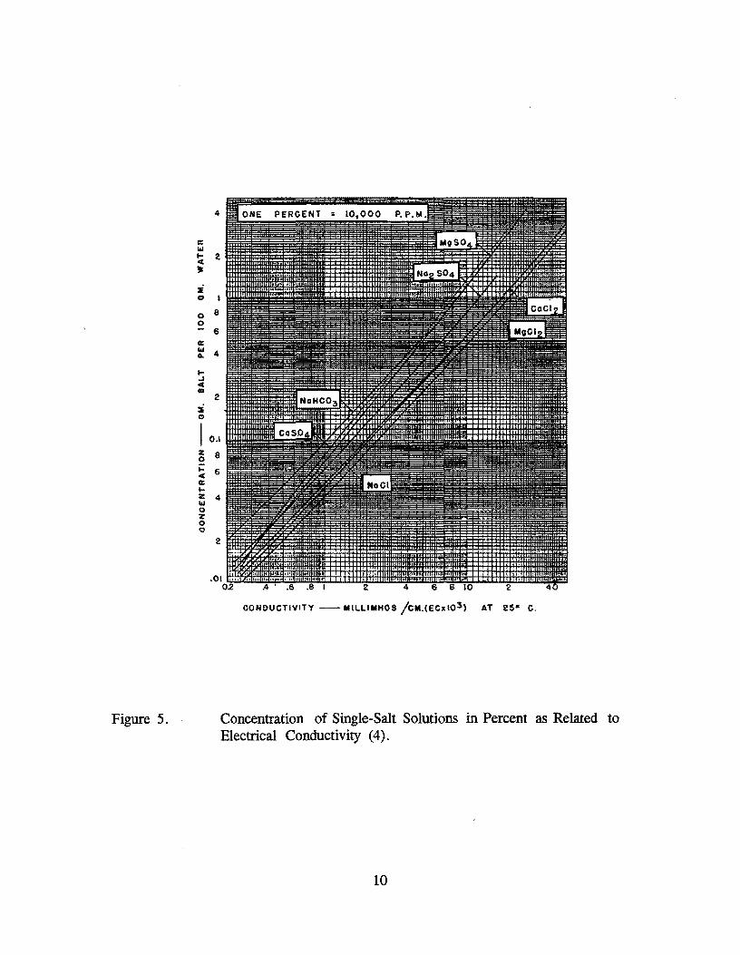
Figure 5.
4
i CI I
o 8 o
...
..I
'" • i c
6
2
I 0.1
~ 8 i: 6
'" G: ... Z 4 III o Z o o
2
OONOUCTIVITY - MILLIMHOS /CM.(EClII03) AT 25- C.
Concentration of Single-Salt Solutions in Percent as Related to Electrical Conductivity (4).
10

Figure 6.
o to :Ii Q)
o
!O
10
3
0.6
0.3 3
CONOUCTIVITY
6 10 30 60
MILLI MHOS/ CM.(ECxI0 3) AT 250 C.
Osmotic Pressure of Saturation Extracts of Soils as Related to Electrical Conductivity (4).
11
Table 1.
°C (OF)
4.4 (40)
10.0 (50)
15.5 (60)
21.1 (70)
26.6 (80)
32.2 (90)
Bureau of Soils Data for Reducing Soil Paste Resistance Readings to Values at 15.5°C (60°F) (4).
Ohms
1.000 3.000 5.000 7.000 9.000
735 2205 3675 5 145 6615
867 2601 4335 6069 7803
1000 3000 5000 7000 9000
1 140 3420 5700 7980 10 260
1294 3882 6470 9050 11 646
4380 7300 10 220 13 140
12
Electrical Conductivity Measurements with Permittivity Probe
The dielectric pennittivity and conductivity meter is a device that measures
the dielectric constant and specific conductivity of various materials (7). This device
can be used to perfonn nondestructive measurements in the field or in the
laboratory. Useful correlations between measured parameters and other physical
soil properties can be made. One aim of this investigation is to relate the dielectric
properties and electrical conductivity measured with this probe to the sulfate
content of the soil under investigation. The dielectric constants of soils and other
solids are between 2 and 4, while the dielectric constants of water is 78. Because of
this difference, the moisture content of soil could be usefully related to the
dielectric constant measurement (7).
MINERALOGYOF CLAYSOILS
The four different clay soils used in this investigation were:
a) Eddy clay loam from the Dallas area alongside FM 1382,
b) . Beaumont clay,
c) Houston Black clay, and
d) Kaolinite.
Other soils samples used were natural soil samples obtained from along IH 45
near Palmer in Northeast Ellis County, and from FM 1382 in Southwest Dallas
County. The exact location where each soil sample along FM 1382 and IH 45 was
obtained is indicated on the maps in Appendix A.
The Eddy clay loam is a very shallow and well drained soil which overlays the
Austin chalk geologic formation (9). The surface layer is about 102 mm (4 inches)
thick, alkaline, and grayish brown in color. The underlying material is white, soft,
chalky limestone (9). Penneability of this soil is low, and the erosion hazard is
severe.
13
The Houston black clay is a moderately well drained soil with a moderately
alkaline surface layer (9). From a depth of 152 mm (6 inches) to 965 mm (38
inches) the soil has a very dark grey to black color. Permeability is very low, and
the available water capacity is high. The soil has a very high shrink-swell potential
with low strength (9).
Both the Beaumont clay and the Houston black clay are vertisols which means
that they are strongly developed soils (10). The most abundant mineral in both of
these soils is dioctahedral smectite which has a 2: 1 mineral structure as shown in
Figure 7. The charge per formula weight is 0.6 to 0.25, and the interlayer contains
exchangeable cations which could be aluminum, iron, or magnesium. Smectites
have a very high surface area that shrinks upon drying and swells upon wetting.
This shrink-swell behavior is most pronounced in the Vertisol order and can lead to
engineering problems when houses, roads, and other structures are built on smectitic
soils (10).
The Eddy clay loam has a mixed mineralogy with smectites, mica, Hydroxy
interlayer smectite (HIS), and kaolinite (11). Mica minerals also have a 2:1 layer
structure, but instead of having only Si4+ in the tetrahedral sites, one fourth of the
tetrahedral sites are occupied by AI3+ which causes one excess negative charge per
formula unit (10). This negative charge is balanced by a monovalent cation,
commonly K+, that occupies the interlayer sites between the 2:1 layers (10). Micas
weather to vermiculites and smectites by losing the interlayer K+. The layer
structure of mica is shown in Figure 8.
Hydroxy-interlayer smectite is smectite with a hydroxy-AI mineral in the
interlayer (between the 2: 1 layers). The combination of the 2: 1 layer with the
hydroxy-AI in the interlayer gives a structure similar to that of chlorite; therefore,
these minerals are also called secondary chlorites (10). The interlayer hydroxy-AI
prevents smectite from shrinking and swelling as it normally would (10).
Kaolinite has a 1: 1 layer structure, is dioctahedral, and contains A13+ in the
octahedral sites and Si4+ in the tetrahedral sites (10) which makes it electrically
neutral. The layer structure is shown in Figure 9. Kaolinite is an abundant mineral
14

BEIDELLITE
MONTMORILLONITE E c: q N . 9
NONTRONITE
Figure 7. Layer Structure of 2:1 Clay Mineral (Smectite) (10).
15

Mica
Figure 8. Layer Structure of Mica Mineral (10).
® o
HYDROXYL
OXYGEN
X o ALUMINUM
o SILICON
z
+-Si, AI
+-AI. Mg, Fe
J-y
Figure 9. Layer Structure of 1:1 Clay Mineral (Kaolinite) (10),
16
in weathered soils (10). Cation exchange capacities and surface areas of kaolinite
are typically low because of the small amount of substitution. Kaolinite is mainly
formed from weathering of primary and secondary minerals that contain large
amounts of Si and AI. Kaolinites form mostly from clay sediments and igneous rock
(10).
Although a consensus of opinion on the most appropriate model of clay
expansion has not been reached yet, the observation that layer silicates,' such as
smectites and vermiculites, approach maximum hydration beyond which they do not
expand, can be explained by a model of H-bonding (12). This model proposes that
the hydration water acts as a dielectric link between the exchangeable cation and
the surface oxygen atoms (12). In vermiculite, the tetrahedral negative charge is
distributed over relatively few surface oxygen atoms, so that an arrangement occurs
where the hydration water is only two molecules thick, as shown in Figure lOa. The
smectite tetrahedral negative charge is distributed more diffusely which favors a
more extended arrangement of dielectric linkages and a necessarily greater
interlayer spacing shown by the structure in Figure lOb. A physically reasonable
explanation of the inability of clays to expand beyond the spacings shown in Figures
lOa and lOb could be that any further reduction in energy due to additional
hydration of exchange cations would be balanced by reduced efficiency of charge
transfer to surface oxygens (12).
a cx:J:J:D b "H "H " : " :
" " H H H H
'S"'O-H-<>-H 0" '0 2 ' "
H-O-H-O" 'H'O ... H' " "
dJxJJ Figure 10. ' Arrangement of H20 Chains Linking a Divalent Exchange Cation
on the Surfaces of a) a 1.5 nm Hydrate of Vermiculite and b) a 2 nm Hydrate of Smectite (10).
17

STABILIZATION OF BASE COURSES WITH LIME
Soils often require stabilization to enhance mechanical stability, to improve
durability, and to reduce volume change potential (13). Compaction is the most
common form of soil stabilization. However, when dealing with high plasticity soils,
compaction alone is often not enough. Alternative soil stabilization techniques are
mostly used when more than 25% of the soil is smaller than 2 J..lm (0.OO2 mm) with
a plastic index (PI) that exceeds 10 (13).
Pozzolanically induced long-term strength gain is achieved by mixing lime into
clay soils. Many clays are reactive, and their strengths can double, and in some cases
even quadruple, upon lime stabilization (13).
When lime is added to clay soils, the divalent calcium cations in the lime
almost always replace the exchangeable cations adsorbed at the clay surface (13).
This cation· exchange results in stabilization and reduction in size of the diffused
water layer. Clay particles approach each other more closely and flocculation occurs.
The lime-soil-water system creates a high pH environment which enhances
flocculation (10). The flocculation leads to increased internal friction which results
in greater shear strength and workability increases due to the change of texture
from a plastic clay to a more sand-like material (13).
The amoupt of lime to be used for the treatment of the subgrade must be
determined by laboratory testing and empirical methods recognized in the literature
(13). The optimum lime content is normally based on strength improvement.
The steps involved in stabilization or modification with lime include
scarification and partial pulverization of the soil, lime spreading, wetting, mixing of
lime with the soil, compaction to maximum practical density, and curing prior to
placing subsequent layers, or a wearing course (13).
FORMATION OF ETTRINGITES
Lime' treatment for stabilization of subgrade soils was used for an
approximately 5 kIn (three mile) section of arterial street in Las Vegas, Nevada.
Two years after construction, signs of distress began to appear in the form of
18

surface heaving and cracking (14). Subsequent investigations showed that heave
developed in the lime-treated soils containing sulfates such as sodium sulfates and
gypsum (calcium sulfates). The heave is mainly due to the growing of disruptive
volumes of hydrous calcium hydroxide sulfate minerals (3). Minerals that were
found in abundance in the heaved areas were thaumasite, a complex calcium
silicate-hydroxide-sulfate-carbonate-hydrate, and ettringite, a calcium-aluminum
hydroxide-sulfate-hydrate mineraL The mechanism of heave was found to be a
complex function of available water, the percentage of soil clay, and cation exchange
capacity (CEC) (3).
The sulfate induced heave problem in lime treated clays did not receive
recognition until the Las Vegas case in 1986, and the interaction of lime and sulfate
bearing clay soils is still not fully understood. A current working hypothesis
proposed by Petry and Little (1) is discussed in the following paragraph.
When lime is added to clay soil, the pH rises and aluminum and siliceous
pozzolans are released to form calcium silicate hydrate (CSH) and calcium
aluminum hydrate (CAH). The presence of sulfates confounds this reaction and
leads to the formation of ettringite, which is an expandable mineral. The formation
of ettringite is favored in low alumina environments. Ettringite is stable in both wet
and dry conditions and can expand to a volume equal to 227 % of the total volume
of the reactant solids (1). Ettringite can be transformed to thaumasite (another
expandable mineral), when a sufficient amount of carbonate and dissolved silica is
present in the soil system at temperatures between 4.5 and 15°C (40 and 59 OF),
19


INTRODUCTION
CHAPTER 3
METHODOLOGY
In this chapte~, the methods used to perfonn various tests to investigate the
heaving problems related to sulfate bearing soils will be outlined. Two major types
of tests were perfonned in this investigation:
a) Expansion tests were perfonned to detennine the expansive properties
of soils that contain natural sulfates and soil that contain added sulfates,
upon hydrated lime stabilization and also upon stabilization with low
calcium fly-ash.
b) Electrical conductivity measurements were perfonned to investigate a
possible relationship between electrical conductivity in soils and the
sulfate content in soils.
The tests were perfonned on two groups of soil samples:
a) Four naturally occurring clay soils which are often encountered in Texas,
namely: Houston black clay, Beaumont clay, Eddy clay, and a kaolinetic
clay. The locations from which these soils were obtained and the
. mineralogy of the clay soils are discussed in Chapter 1.
b) Soil samples from various locations along Interstate Highway (IH) 45
and Farm to Market Road (PM) 1382, near Dallas, Texas, where
heaving problems have been encountered. These soils vary from sandy
loams to heavy clays.
Additional tests that were perfonned to gain a better understanding of the soil
mineralogy and behavior are listed below.
21

1) Cation exchange capacity (CEC) determination
2) Detennination of soluble sulfate content
3) Dielectric constant determination
METHOD FOR DETERMINATION OF EXPANSION OF SULFATE BEARING
CLAY SOILS
A set of experiments was perfonned to detennine the amount of expansion
that occurs in soils containing different amounts of natural sulfates, added sulfates,
and hydrated lime. The aim was to detennine the amount of sulfates that causes
expansion in lime stabilized soils. The expansion tests were conducted on 4 different
clay soil samples and various samples obtained from IH 45 and FM 1382, both in
Dallas County, near Ceda Hill, Texas. These soils were chosen because they are
frequently encountered in the Texas area, and Eddy clay has a history of swelling
excessively when stabilized with lime. The expansion of several other soil samples
along IH 45 and FM 1382 near Palmer in Dallas County was also investigated
because heaving problems were encountered along these roads.
The way in which these experiments were perfonned is as follows:
1) Soil samples were collected from different locations in Texas, as
described previously.
2) The samples were sun dried and crushed to pass the 0.425 mm (no. 40)
sieve.
3) After drying and crushing, 3 kg of each of the 4 clay soil samples were
mixed with lime, water, and calcium sulfate (CaS04.2HzO - gypsum) in
ratios described in Table 2. The soil was weighed into a container after
which the lime and then the sulfates were added. The container was
closed tightly and turned over for 2 minutes to mix the dry ingredients.
After mixing the dry ingredients, 15% water was gradually added to the
mix while the soil was constantly stirred to ensure a unifonn mixture.
Fifteen percent water was used because when mixed with the soil, it
22

Table 2. Ratios of Lime and Sulfates Added to the Four Clay Soil Samples.
·Sample Amount Amount Amount Amount Number of of of of
soil lime sulfates water (kg) (%) (%) (%)
1 3 0 0 15
2 3 0 0.2 15
3 3 0 0.4 15
4 3 0 0.6 15
5 3 0 0.8 15
6 3 6 0 15
.7 3 6 0.2 15
8 3 6 0.4 15
9 3 6 0.6 15
10 3 6 0.8 15
• These 10 compositions were made up for each of the 4 clay soil samples, which resulted ina total of 40 samples.
23

resulted in a workable consistency which facilitated subsequent
compaction tests. Previous investigation (3) showed that 0.8 % sulfates by
weight seemed to be a relatively large amount of sulfates that occur
naturally in most soils in the Texas area. Therefore, up to 0.8 % of
sulfates were used in these mixes. Six percent lime is an average amount
added to most clay soils in order to stabilize the soil. For this reason, the
same amount of lime was added to the mixes in this investigation. The
soil samples obtained from IH 45 and FM 1382 were mixed with 6 %
lime without the addition of sulfates. However, some of the soil samples
contained natural sulfates. Three samples from each location were mixed
. with 6 % lime, while one sample was not mixed with lime and served as
a control sample. The samples were mixed with 15% water prior to
compaction.
4) After the soil, lime, sulfates and water had been mixed, the samples
were stored at 50% relative humidity at 25°e to cure for a period of 12
hours.
5) The samples were then compacted using the standard proctor
compaction method (15).
6) Each of the compacted cores was wrapped in a rubber membrane with a
porous stone at the top and the bottom of each core.
7) . The core samples were then placed in pans filled with 2 cm of water to
allow the samples to soak up the water.
8) This whole experimental setup was placed in a lOoe constant
temperature room with a controlled relative humidity of 100%. These
cold, wet conditions seem to encourage the formation of ettringites (1).
9) . The samples were kept under these conditions to expand freely for a
period of 3 months during which the expansion of the samples was
frequently monitored.
24

METHOD FOR DETERMINING ELECTRICAL CONDUCTIVITY WITH
PERMITTIVITY PROBE AND THE EPA METHOD NO. 9050
Because of sulfate related heave in lime stabilized soils, a need developed to
determine the sulfate content of in situ soils. Electrical conductivity tests were
performed to investigate a possible relation between the amount of sulfates and the
electrical conductivity of soil samples. Two methods were used for determining the
electrical conductivity. The first method was a standard approved EPA procedure
(16) and served as a control for a proposed method by a permittivity probe which
could be used for field determination of electrical conductivity of the in situ soil.
The following steps outline the procedure followed:
1) Samples of each of the four clay soils were mixed with lime and sulfates
in ratios outlined in Tables 3a, b, and c. Each of the combinations 1
through 18 was repeated for each of the four clay soils under
investigation.
2) For the electrical conductivity measurements with the permittivity probe,
the samples were diluted to a 1:2 soil:water ratio with de-ionized water.
Another set of conductivity measurements was taken on the samples
diluted to a 1:4 soil:water ratio because the conductivity of low soluble
.salts like sulfates are influenced by the dilution (8). The permittivity
probe measured electrical conductivity directly on the soil slurry.
3) Electrical conductivity measurements according to the EPA method were
performed on a water extract taken from a 1:2 soil:water ratio mixture.
The specific conductance of a sample was measured using a self
contained Wheatstone bridge-type conductivity meter (15). Whenever
possible, the samples were analyzed at 25°C. If samples were analyzed at
different temperatures, temperature corrections were made and results
reported at 25°C.
4) Samples of soil obtained along IH 45 and FM 1382 were subjected to
electrical conductivity tests only by the EPA method. No sulfates or lime
were added to these samples.
25

Table 3a.
Table 3b.
Composition of Soil Samples on which Electrical Conductivity Measurements were Performed (Samples Containing Natural Soil and Sulfates).
Sample No. Amount of Sulfates (%)
1 0
2 0.2
3 0.4
4 0.6
5 0.8
6 1.0
Composition of Soil Samples on which Electrical Conductivity Measurements were Performed (Samples Containing Natural Soil, Sulfates and Chlorides).
Sample No. Amount of Amount of Sulfates (%) Chlorides (%)
7 0 1.0
8 0.2 0.8
9 0.4 0.6
10 0.6 0.4
11 0.8 0.2
12 1.0 0
26
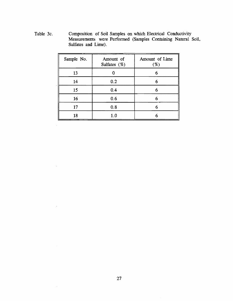
Table 3c. Composition of Soil Samples on which Electrical Conductivity Measurements were Performed (Samples Containing Natural Soil, Sulfates and Lime).
Sample No. Amount of Amount of Lime Sulfates (%) (%)
13 0 6
14 0.2 6
15 0.4 6
16 0.6 6
17 0.8 6
18 1.0 6
27

l\1ETHODFOR INVESTIGATING SEVERAL LOW CALCIUM FLY-ASHES AS
ALTERNATIVESTABILIZERS
An alternative stabilizer is needed whenever excessive heave is expected from
sulfate bearing soils that are stabilized with lime. Most commonly used forms of
lime used for stabilization are hydrated high calcium limes (13). The calcium reacts
with the sulfates in the soil to form ettringites, as discussed in Chapter 1. Low
calcium fly-ashes have been proposed as alternative stabilizing agents for sulfate
bearing soils. The low calcium fly-ashes used in this investigation were:
1) Sandow from Rockdale, distributed by The Money Resources in San
Antonio, Texas, which contains 13% calcium.
2) Montecello from Mt. Pleasant, distributed by the Lafarge Corporation m
Dallas, Texas, and containing 8.47% calcium.
3) Big Brown from Fairfield, distributed by the Lafarge Corporation m
Dallas, Texas, and containing 9.8% calcium.
Each of these low calcium fly-ashes was mixed with samples of the four clay
soils used in this investigation as well as Sample No.7 from FM 1382 which showed
excessive heave after lime stabilization. The method followed to perform these
expansion tests is similar to the method outlined for determination of expansion in
soil samples discussed previously in this chapter. However, no sulfates were added
to the soil prior to compaction, and the evaluation was based on the natural sulfate
content of the various soil samples.
l\1ETHODS BY WHICH SUPPLEl\1ENTARY TESTS WERE PERFORl\1ED
Cation Exchange Capacity Determination
The CEC of all soil samples was determined by the EPA method No. 9081
(17). A soil sample is mixed with an excess of sodium acetate solution, resulting in
an exchange of the added sodium cations for the matrix cations. Subsequently, the
sample is washed with isopropyl alcohol. An ammonium acetate solution is then
28

added which replaces the adsorbed sodium with ammonium. The concentration of
displaced sodium is then detennined by atomic absorption, emission spectroscopy,
spectrophotometer, or an equivalent means (17).
Method for Detennination of Soluble Sulfate Content
EPA method No. 9038 (18) was used to detennine the amount of soluble
sulfates in the soil samples. The naturally occurring soluble sulfates in each of the
four clay soil samples, as well as each of the samples obtained from PM 1382 and
IH 45, were detennined. The procedure involves converting the sulfate ion to a
barium sulfate suspension under controlled conditions. The resulting turbidity is
detennined by a mephelometer, filter photometer, or spectrophotometer and
compared with a curve prepared from standard sulfate solution (18).
Method for Determination of Dielectric Constants
Dielectric constants were only measured for the four clay soil samples under
investig~tion. The dielectric constant measurement was made directly after the
electrical conductivity measurement with the permittivity probe on the soil slurry
with a 1:2 soil to water ratio. The measurement was made with the same probe as
the one used for conductivity measurements at different frequencies ranging from 0
to 3 Gigahertz.
29


CHAPTER 4
RESULTS FROM EXPANSION TESTS
INTRODUCTION
This chapter presents and discusses the results obtained from expansion tests.
Expansion tests have been performed on samples obtained along FM 1382 and IH
45 and on the four clay soil samples. The results from expansion tests on samples
obtained from FM 1382 and IH 45 are discussed separately from the results
obtained from the four clay soil samples. The most important difference between
these two groups of samples is that the samples from FM 1382 and IH 45 contain
only natural sulfates, while calcium sulfate (gypsum) was added in different
quantities to the four clay soils, as described in the previous chapter.
In each case, the percentage of volumetric expansion was calculated by
measuring the percentage increase in the circumference and height of the sample.
RESULTS OF EXPANSION TESTS PERFORMED ON SAMPLES FROM m 45
ANDFM 1382
The expansion over time of soil samples from FM 1382 and IH 45 is shown in
Figures 11 and 12, respectively. Each data point on Figures 11, 12, and 13
represents the average amount of volumetric expansion calculated from four
samples of the same type and location. Figures 11a and 12a represent the expansion
of soil samples containing 6% hydrated lime, and Figures llb and 12b represent
samples containing no lime. From Figure 11a, it is evident that the sample marked
FM 1382 Sample No.7 which contained 6% lime, expanded more than any of the
other samples. This sample also expanded the most of all the samples containing no
lime (Figure llb). Apart from showing the greatest expansion upon lime
stabilization, the sample marked FM 1382 Sample No.7 had the highest amount of
sulfates (0.8% with a 1:0.5 soil: water ratio). From Figure 12a, it is evident that all
samples from IH 45 responded well to lime stabilization, and the amount of
expansion was between 0 and 2 %. These same samples from IH 45 expanded
31
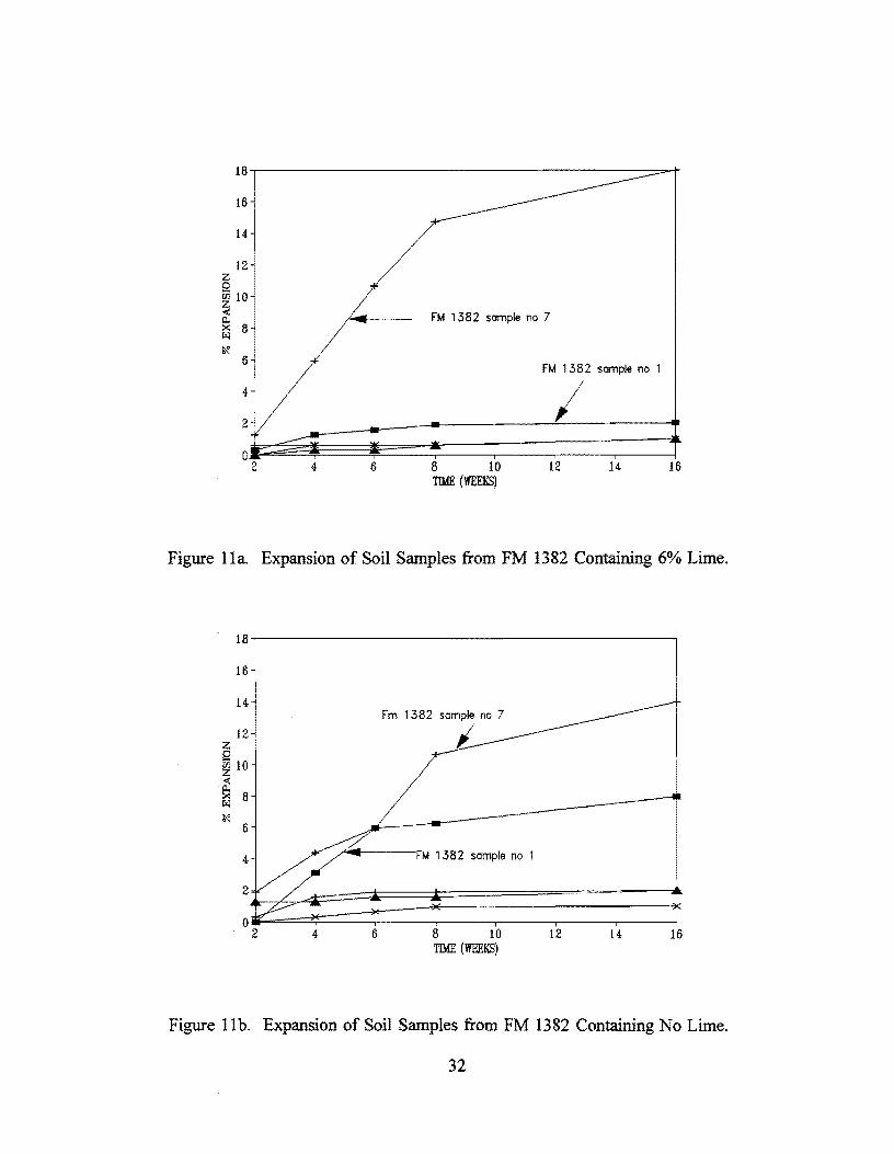
18
16 J
14
12 Z 0 m 10 ~ 0.. X 8 f;il
~ 6
4
2
0 2 4 6
FM 1382 sample no 7
FM 1382 sample no 1
8 10 TIME (WEEKS)
I 12 14 16
Figure Ila. Expansion of Soil Samples from FM 1382 Containing 6% Lime.
18
16
14j Fm 1382 sample no 7
12 . i z 0 m 10 ~ ~ 8 f;il
~ 6
4 FM 1382 sample no 1
2
4 6 B 10 12 14 16 TIME (WEEKS)
Figure lIb. Expansion of Soil Samples from FM 1382 Containing No Lime.
32

18
16
14-
12 Z 0
~ 10
~ 8 I"il
~ 6
4
2 -0 2 4 6 8 10 12 14 16
TIME (WEEKS)
Figure 12a. Expansion of Soil Samples from IH 45 Containing 6% Lime.
18,.----------------------------------------~
16
14
12 Z o ~ 10
~ 8
6
4,
4 6
H 45 sample no 3
8 10 TIME (WEEKS)
IH 45 sample no 2
12 14 16
Figure 12b. Expansion of Soil Samples from IH 45 Containing No Lime.
33
14 -12
10 ".....
~ '-' 8 c 0
'00 c a 6 D.. X
UJ
4 -2 -0 I-
0 0.1 0.2 0.3 0.4 0.5 0.6 0.7 0.8 0.9 Sulfate content (%)
Figure 13a. Expansion of Soil Samples Containing 6% Lime VS, Sulfate Content.
14
12
10 -"" ~ '-' 8
s::: 0 'iii !: 0 6 D.. x
I.JJ
.a.
2
0.1
-
0.2 0.3 0.4 0.5 0.6 Sulfate content (%)
-
0.7 0.8 0.9
Figure 13b. Expansion of Soil Samples Containing No Lime vs. Sulfate Content.
34

between 2 and 6 % when not lime stabilized. None of these samples contained
significant amounts of sulfates.
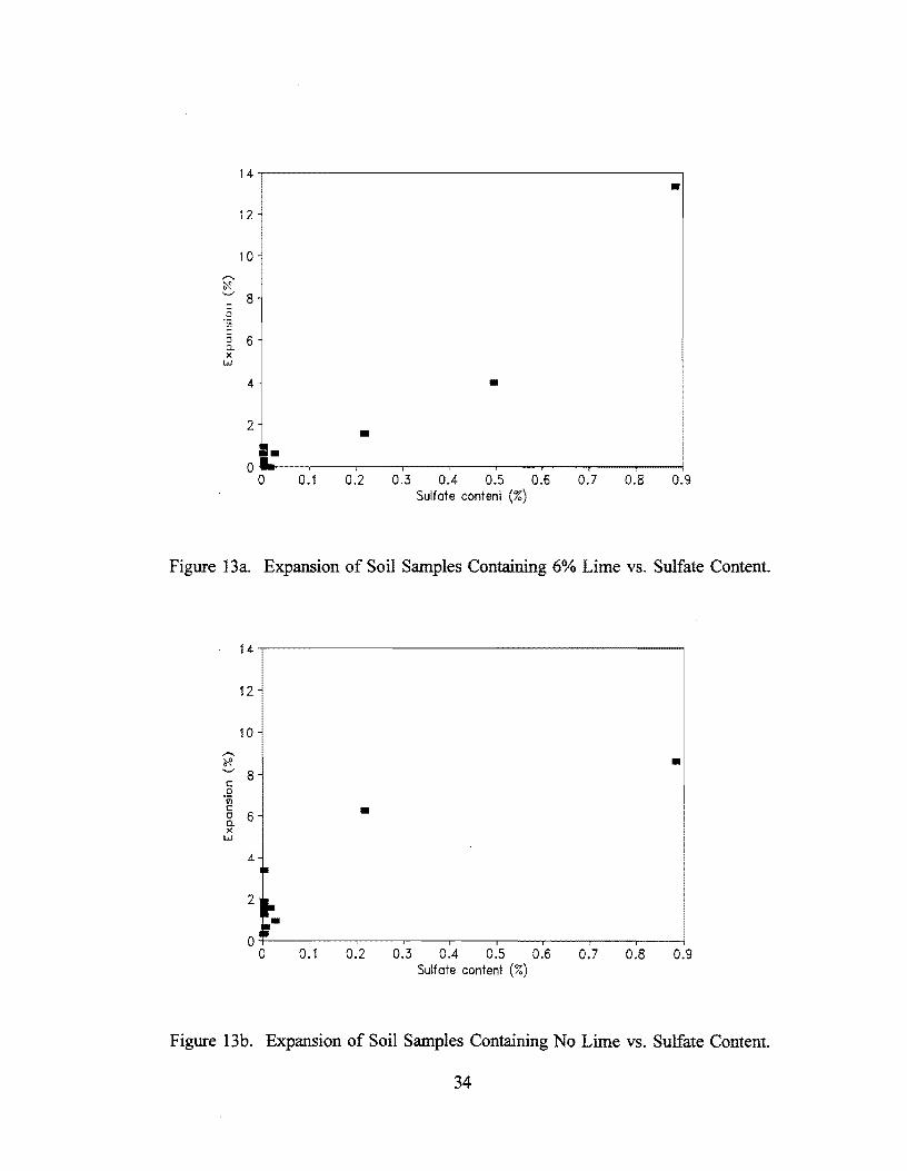
Figures 13a and b show the relation between the expansion of the samples and
the natural sulfate content of the soil samples containing 6% lime and soil samples
containing no lime. This figure shows that soil samples containing higher amounts of
sulfates experienced greater expansion. Although it is evident from Figures 13a and
b that expansion increases with increasing sulfate content, a linear regression was
performed in order to test whether a flat line could adequately describe the data. If
a flat line could be fitted better than a sloping line, this would indicate that,
statistically, there is no relationship between the amount of expansion and the
sulfate content of the samples. The hypothesis that a flat line fit is adequate for this
data was rejected at a 99% confidence level (19). This indicates that there is a
definite statistical relation between the natural sulfate content of soils and the
amount of expansion that occurs after lime stabilization.
Figure 14 is a photograph of the expansion of samples that do not contain
lime. The sample on the left contains less that 0.2 % sulfates, and the sample on the
right contains 0.8% sulfates. The sample with the highest sulfate content showed the
greatest expansion.
Figure 15 shows 3 samples that were stabilized with lime. The two samples on
the left expanded approximately 14% and contained 0.8% SUlfates, while the sample
on the right is still its original size and contained less than 0.2%·sulfates. Once
again, the samples with the highest sulfate content showed the greatest expansion.
Figure 16 shows 2 samples which both contain 0.8% sulfates. One sample was
stabilized with 6% lime, and the other contains no lime. The sample containing lime
expanded 6% more than the sample that was not stabilized with lime.
35

Figure 14. Expansion of Samples Containing No Lime. Sample on Left Contains Less than 0.2% Sulfates aftd Sample on Right 0 .8% Sulfates.
36

Figure 15.
No L'~E
Samples Containing 6% Lime. The Two Samples on the Left Contain 0.8% Sulfates and Expanded 18%. The Sample on the Right Contain Less than 0.2% Sulfates and is Still Close to Original Size.
37
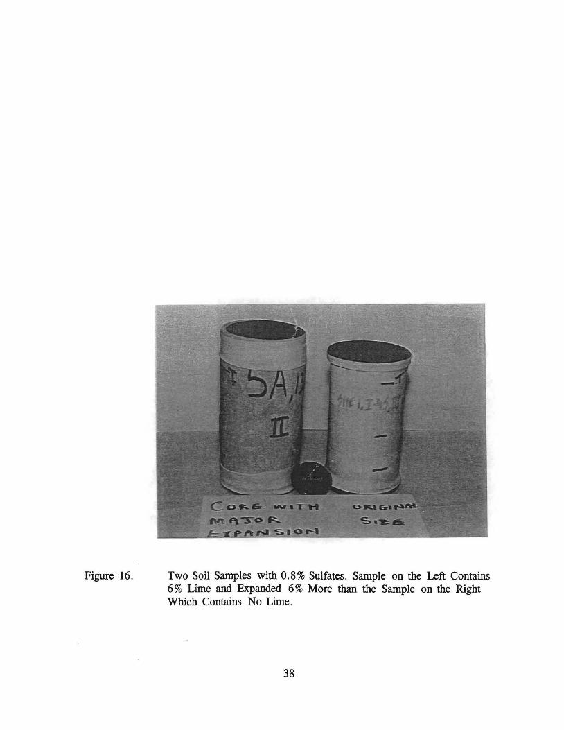
Figure 16. Two Soil Samples with 0.8% Sulfates. Sample on the Left Contains 6 % Lime and Expanded 6 % More than the Sample on the Right Which Contains No Lime.
38

RESULTS OF EXPANSION TESTS PERFORMED ON CLAY SOIL SAMPLES
As described in Chapter 2, ten samples of each clay soil were prepared with
different amounts of sulfates and lime. Figures 17a to c show the expansions of a
Beawnont clay, an Eddy clay, and a Houston black clay, with time. This chapter
presents only the results of the soil samples that contained no added sulfates. The
addition of sulfates had no apparent effect on the expansion of the samples both
with and without lime stabilization. The samples which contained added sulfates
behaved in much the same way as the samples without added sulfates.
The kaolinitic clay samples expanded so drastically within the first week that
the samples completely came apart and further expansion on the samples could,
therefore, not be measured. Figure 17d is a photograph of the kaolinitic samples
after one week. The kaolinitic clay contained the highest percentage of natural
sulfates (0.06% with a 1:2 soil:water ratio) of the four clay samples.
The Beawnont clay contained the second highest percentage of sulfates
(0.01 % with a 1:2 soil:water ratio). The means (Figure 17a) were compared with a
two-sample t-test (19), and all but the first two measurements were found not to be
significantly different with a 95 % confidence level. This indicates that there is no
significant difference in the amount of expansion between the lime stabilized and
un-stabilized samples. The ineffectiveness of the lime stabilization could be due to
the relatively high natural sulfate content of the Beaumont clay.
The other two clay soils, the Eddy clay and the Houston black clay, contain
negligible amounts of natural sulfates and, in this case, the samples containing 6%
lime expanded less than the samples containing no lime. In the case of the Houston
black clay, the samples containing no lime showed much greater expansion than the
stabilized samples, especially between the sixth and the twelfth week.
39
10
9
B
7 c:
6 / 0 "iii c: 0 5 0-X I w
~ ~ :1 1 ~
O+[----~I----~I----~I~--~I----~I --~ o 2 4 6 8 10 12
Time (weeks)
1--- no lime -*- 6 % lime
Figure 17a. Expansion of Beaumont Clay Samples vs. Time.
10~------------------------------------------~
9
8
7
5 6 iii c: li 5
~ :J 2,
1..!
O+-------,------.-------,-------r------.-----~
o 2 4 6 B 10 12 Time (Weeks)
1--- no lime -*- 6 % lime
Figure 17b. Expansion of Eddy Clay Samplesvs. Time.
40

10 ~----------------------------------------~
9
8
7
§ 6 'iii c 8.. 5 x w 4 ~
3
2
O+-----~------_r------~----~------_r----~
o 2 4 6 8 10 12 time (weeks)
1--- no lime ~ 6 % lime
Figure 17c. Expansion of Houston Black Clay Samples vs. Time.
Figure 17d. Expansion of Kaolinitic Samples.
41

CONCLUSIONS
From Figure 13, it is evident that the sulfate content is related to the amount
of expansion encountered in soil samples from FM 1382 and IH 45. As the
sulfate content increases, the amount of expansion increases. This expansion
could be due to the reaction between the calcium in the lime and the sulfates
in the soil which form ettringite, an expandable mineral described in Chapter
1.
Unstabilized soils which contained relatively high amounts of sulfates (>0.2%
with 1:0.5 soil water ratio) showed greater expansions than un-stabilized soils
containing small amounts of sulfates «0.2% with 1:0.5 soil water ratio)
(Figure 14).
In some cases, soil samples with high sulfate contents that were stabilized with
lime expanded more than samples with the same sulfate content that were not
stabilized with lime, as can be seen in Figure 16. For this reason, it might be
advantageous not to stabilize sulfate bearing soils at all, or to use an
alternative stabilizer rather than to stabilize these soils with lime.
The addition of sulfates has no effect on the expansion of the soil samples,
regardless of whether the samples contained lime or not. It seems like
ettringites do not form in cases where the natural sulfate content is low, even
though up to 1 % sulfates were added to the soiL
Of the four clay samples under investigation, the samples with the highest
sulfate content (Kaolinite, Figure 17d) expanded most. Samples that did not
contain natural sulfates expanded less if lime stabilized than the unstabilized
samples.
42
CHAPTER 5
RESULTS FROM ELECTRICAL CONDUCTIVITY
MEASUREMENTS
INTRODUCTION
This chapter presents the results obtained from electrical conductivity
measurements performed by the standard EPA procedure and a permittivity probe (as
outlined in Chapter 2). In each case, the electrical conductivity is related to the sulfate
content of the soil and also to the total amount of soluble salts for a known soil:water
ratio. Soluble salts are those salts that dissolve when a known amount of water is added
to the soil. If more water is added to the soil, more of the salt in the soil dissolves in the
water. For this reason, the soil:water ratio is an important parameter that should always
be reported when salt concentrations are reported. The soil:water ratio is determined by
proportions of the weight of the soil and the water.
The sulfate content, as measured by the EPA procedure for the determination of
total soluble sulfates, is presented for each soil under investigation. Electrical
conductivity measurements were taken on the four clay soil samples and also soil
samples from FM 1382 and IH 45. The sulfate content of the soils, as determined by the
EPA procedure, is presented first. After that, the electrical conductivity for different
sulfate contents is presented.
RESULTS FROM SOLUBLE SULFATE DETERMINATION
Tables 4a and b contain the results from the determination of soluble sulfates for
the different soil samples. The total amount of sulfates in soils from FM 1382 and IH 45
cannot be compared to the amount of sulfates in the four clay soils since the sulfate
determination was performed at different times and was not performed at the same
soil:water ratio. As a consequence of the greater water content used with the four clay
soils, the amount of soluble salts in the pore water is expected to be greater by an
undetermined amount than in the pore water in the soils from IH 45 and FM 1382. As
previously mentioned, gypsum is one of the least soluble salts, and the amount of
gypsum detected in soils is highly dependent on the soil:water ratio.
43

Table 4a. Amount of Soluble Sulfates in the Four Clay Soil Samples.
Material Type Amount of Soluble Sulfates (meq/l) 1:2 soil:water ratio
Eddy Clay 0.4
Houston Black Clay 1.1
Beaumont Clay 1.2
Kaolinite 12
Table 4b. Amount of Soluble Sulfates in the Soil Samples Obtained from FM 1382 and IH 45.
Location Sample No. Amount of Soluble Sulfates (meq/l) (1:2 soil:water ratio)
IH 45 1 0.7
2 0.5
3 0.5
4 0.7
5 0.5 i
6 1.3
7 0.5
8 0.6
i 9 0.5
I 10 2.1
FM 1382 1 45.5
2 3.5
3 0.4
4 0.7
5 5.6
6 103.4
7 184.
44

There is a general tendency to believe that the light colored clays, like the
kaolinitic clay and the Eddy clay from FM 1382 Soil Sample No 7, have the highest
amount of soluble sulfates. However, this is not always true since the Eddy clay which
was used as one of the standard clay soil samples is light colored but has a low sulfate
content of 0.4 meq/l.
RESULTS FROM ELECTRICAL CONDUCTIVITY MEASUREMENTS ON SOIL
SAMPLES OBTAINED FROM IH 45 AND FM 1382
The results from the electrical conductivity for these samples were obtained only
by the EPA procedure with a 1:20 soil:water ratio. Figure 18 shows how the electrical
conductivity increases as the sulfate content of the soils increases. In this case the
electrical conductivity is related to the natural sulfate content in the soils since no
sulfates were added to these samples. The hypothesis that a flat line fits the data from
Figure 18 adequately was rejected with a 99% level of confidence. This indicates that
there is a statistical relation between the sulfate content and the electrical conductivity of
the soils. A. regression analysis was performed to obtain an equation that describes the
relation between electrical conductivity and the sulfate content in the soil (19). The
equation that fit the data best with a correlation
coefficient of 0.9985 is:
EC exp(0.799 + 0.014 x Sulfate Content)
where EC is the electrical conductivity in mS/cm. The regression line that fits the data
best is shown in Figure 19.
RESULTS FROM ELECTRICAL CONDUCTIVITY MEASUREMENTS ON
FOUR CLAY SOILS
Electrical conductivity measurements for the Eddy, Beaumont, Houston black, and
Kaolinitic clay for both methods, EPA procedure and permittivity probe, are
presented in Figures 20a to d. For the Eddy, Houston black, and Kaolinitic clay, the
electrical conductivity at a sulfate level of 1 % reaches a value between 5 and 8
mS/cm. The electrical conductivity of the Beaumont clay does not seem to increase as
45

30,---------------------------------------~
,....." 25 E (,)
"Vl
520 :?: :~ 1) 15 ::l
1J C o (,)
"6 10 . 2 '-
1)
~ 5
•
•
•
OT;----~'--_.'----,'----r' ---.'----,'----'r---,'--~
Figure 18.
o 0.1 0.2 0.3 0.4 0.5 0.6 0.7 0.8 0.9 Sulfate content (%)
Relation Between Electrical Conductivity and Natural Sulfate Content of Soil Samples from FM 1382 and IH 45.
30.---------------------------------------~
>-"-+-.;;:
i 15 :::l 1J C o (,)
"6 10 u :£ u
~ 5
•
OT----r---.----,---~--_,----r_--~--_.--~
Figure 19.
o 0.1 0.2 0.3 0.4 0.5 0.6 0.7 0.8 0.9 Sulfate content (%)
Regression Line for Electrical Conductivity and Sulfate Content.
46

16,---------------------------------------------~
""" 14 E o
';;) 1 2 E '-'
>- 10 .~ (j 8 -5 c:: 8 6 "5 .~ 4 l...
(j ~
-t..,l 2
0.1 0.2 0.3 0.4 0.5 0.6 0.7 0.8 0.9 Sulfate Content (%)
1--- permittivity probe --*- EPA Procedure
Figure 20a. Electrical Conductivity vs. Sulfate Content of a Beaumont Clay.
"""' E 0
"-.. tn E '-'
1::-~ 0 ::l "0 c:: 0 u 0 .2 l...
(j -ill W
10
9
8
7
6
5
4
3
2
0.1 0.2 0.3 0.4 0.5 0.6 0.7 0.8 0.9 Sulfate Content (%)
I --- permittivity probe --*- EPA Procedure
Figure 20b. Electrical Conductivity vs. Sulfate Content of an Eddy Clay.
47

10,-----------------------------------------------,
9
E u 8
'" (f)
E 7 '-'
>.. 6
~ g 5 "0 § 4 u "0 3 .~ I..
U 2 Q)
W
0 0
Figure 20c.
0.1 0.2 0.3 0.4 0.5 0.6 0.7 0.8 0.9 Sulfate Content (%)
1--- permittivity probe ""'*- EPA Procedure
Electrical Conductivity vs. Sulfate Content of a Houston Black Clay.
10,-----------------------------------------------,
9
E u 8
'" (f)
E 7 '-'
~ 6 ~ g 5 "0
§ 4 u "0 3 .~ I..
Q 2 Q)
W
0.1 0.2 0.3 0.4 0.5 0.6 0.7 0.8 0.9 Sulfate Content (%)
1--- permittivity probe ""'*- EPA Procedure
Figure 20d. Electrical Conductivity vs. Sulfate Content of Kaolinite.
48

much with an increase in sulfate content, but shows a sudden increase to about 13
mS/cm between sulfate contents of 0.8% and 1%.
Electrical conductivity measurements with two different methods, the permittivity
probe and the EPA procedure, seem to correspond quite well to each other. In most
cases, the results obtained from the EPA procedure are slightly higher than those
obtained by the permittivity probe. A statistical t·test showed that the difference between
the electrical conductivity values determined by the EPA procedure and the permittivity
probe are insignificant The test was performed at a 95% level of confidence.
The effect that salts other than sulfates had on the electrical conductivity was also
investigated. Figure 20e shows how addition of calcium chloride affected the electrical
conductivity. As the calcium chloride decreased from 1% to 0% and the sulfate content
increased from 0% to 1%, the electrical conductivity decreased from about 14 mS/cm to
about 7 mS/cm. This indicates that the electrical conductivity for the calcium chloride is
generally higher than for sulfates. Even though the total salt concentration stayed
constant at 1 %, the electrical conductivity decreased because of the lower maximum
electrical conductivity of sulfates compared to calcium chloride. All the electrical
conductivity values for different sulfate contents for the fourc1ay soils were
superimposed in one graph, shown in Figure 21. A regression was performed in order to
obtain an equation that explains the relation between electrical conductivity and sulfate
content in soils. Although more complex equations were considered, a straight line
seemed to have the best fit. The relation between electrical conductivity and sulfate
content can be represented by the following equation:
where
y=mx+c
y = electrical conductivity (mS/cm)
x = sulfate content (%)
m = Slope of line (5.331) . -
c = Intercept (0.679)
This equation yielded a coefficient of determination of 0.61.
49

16,-----------------------------------------------
,-... 15 E ~ 14 tf';
E 13 '-'
£ 12 .~ () 11 -6 6 10 u 15 '-' :E '-' Q)
Q 7
Figure 20e.
0.1 0.2 0.3 0.4 0.5 0.6 0.7 0.8 0.9 Sulfate Content (%)
0.9 0.8 0.7 0.6 0.5 0.4 0.3 0.2 0.1 Calcium chloride Content (%)
1--- Beaumont ~ Eddy -+- HBC --:IIIIr KaQtinite
o
Electrical Conductivity vs. Chloride and Sulfate Content.
16~----------------------------------------------,
Figure 21.
0.1 0.2 0.3 0.4 0.5 0.6 0.7 0.8 0.9 Sulfate Content (%)
1--- Beaumont ~ Eddy --:IIIIr HBC -+- Kaolinite
Electrical Conductivity Values of the Four Clay Soils vs. Sulfate Content.
50

The reason for determining a regression equation is to be able to predict the most
probable value of electrical conductivity at a given sulfate content for different kinds of
soil. Therefore, it is reasonable to detennine an average electrical conductivity at each
sulfate content for the different soils. This average value of electrical conductivity is then
used to detennine a regression equation with an improved fit. This can be clearly seen
by comparing Figures 21 and 22 where Figure 21 presents all the electrical conductivity
data points for different soils, and Figure 22 presents only the mean values of electrical
conductivity for different soils. Table 5 presents the means calculated from the four
values of electrical conductivity for the four different soils at different sulfate contents.
The corresponding standard variations are also listed in this table.
J f . ()
"(f)5 f
'-'
• •
• •
D+---~---r--~----.---~--~---r---'---'r---. o 0.1 0.2 0.3 0.4 0.5 0.6 0.7 0.8 0.9
Sulfate Content (%)
Figure 22.
I • Average EC - Regression line
Regression Line Fitted through Mean Values of Electrical Conductivity for Different Sulfate Contents.
51
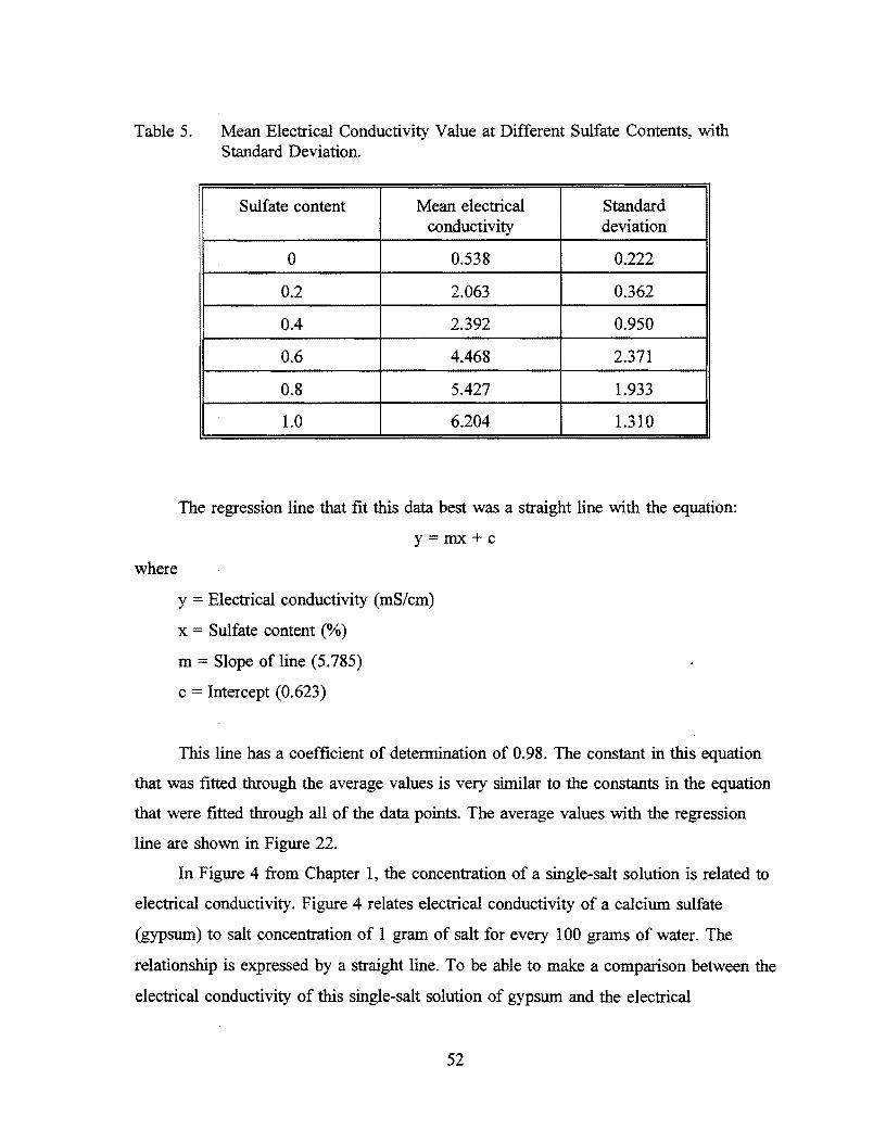
Table 5. Mean Electrical Conductivity Value at Different Sulfate Contents, with Standard Deviation.
where
Sulfate content Mean electrical Standard conductivity deviation
0 0.538 0.222
0.2 2.063 0.362
0.4 2.392 0.950
0.6 4.468 2.371
0.8 5.427 1.933
1.0 6.204 1.310
The regression line that fit this data best was a straight line with the equation:
y=mx+c
y = Electrical conductivity (mS/cm)
x Sulfate content (%)
m Slope of line (5.785)
c = Intercept (0.623)
This line has a coefficient of detennination of 0.98. The constant in this equation
that was fitted through the average values is very similar to the constants in the equation
that were fitted through all of the data points. The average values with the regression
line are shown in Figure 22.
In Figure 4 from Chapter 1, the concentration of a single-salt solution is related to
electrical conductivity. Figure 4 relates electrical conductivity of a calcium sulfate
(gypsum) to salt concentration of I gram of salt for every 100 grams of water. The
relationship is expressed by a straight line. To be able to make a comparison between the
electrical conductivity of this single-salt solution of gypsum and the electrical
52

conductivity of a soil solution containing different percentages of gypsum, it is necessary
to make sure that the salt:water ratio in each case is the same. In the case of the soil
solution with sulfates, a 1:2 soil:water ratio was used with the addition of sulfates
varying from 0 to 1 %, according to the weight of the soiL Using a 1:2 soil:water ratio
with 100 grams of water suggests that the weight of the soil is 50 grams, and one
percent sulfates added to 50 grams of soil is 0.5 grams. Therefore, 0 • .5 grams of sulfates
in 100 grams of water is equivalent to 1% sulfates. In the same way, it can be calculated
that 0.8% of sulfates correspond to 004 grams of salt in 100 g of water, 0.6% to 0.3
grams, 004% to 0.2 grams, and 0.2% to 0.1 gram. By entering Figure 4 in Chapter 1 at
the calculated salt concentrations, the corresponding electrical conductivity values for a
single-salt solution can be obtained. However, to obtain these values it is assumed that
the line representing calcium sulfate can be extended linearly. The values are tabulated in
Table 6. Electrical conductivity values corresponding to gypsum content in a soil
solution, as calculated with the regression equation previously stated, are also presented
in Table 6 ..
Table 6. Comparison between Electrical Conductivity Measurements of Single-Salt Solution and Soil Solutions at the Same Sulfate Concentration.
Sulfate Electrical Conductivity Electrical Conductivity Concentration of Single Salt Solution of Soil Solution
(%) (mS/cm) (mS/cm)
0 0 0.62 ± 0.24
0.2 1 1.77 ± 0.39
004 2 2.93 ± 1.01
0.6 3 4.09 ± 2.53
0.8 4 5.25 ± 2.06
1.0 5 6040 ± lAO
53

From· this table, it can be seen that the regression equation for soil solutions
containing sulfates yields values that are in close correspondence with the values
obtained from electrical conductivity measurements on single-salt solutions. The
electrical conductivity seems to be slightly higher in the case of the soil solution when
compared to measurements on single-salt solutions. The electrical conductivity seems to
be slightly higher in the case of the soil solution when compared to the electrical
conductivity obtained from the single-salt solution. This may be due to the fact that there
are other salts and impurities present in the soil solution which increase the conductivity
potential of the solution. A 90% confidence interval was added to the values obtained by
using the regression equation. For the lower sulfate contents, the confidence interval is
small; however, for the higher sulfate concentrations, the interval tends to get quite large.
WATER CONTENT OF THE IN SITU SOIL
The regression models developed in this chapter relate electrical conductivity to
sulfate content and are dependent on the soil:water ratio of the paste used to measure
electrical conductivity. The two regression models were developed for 1:2 and 1 :20
soil:water ratios, respectively. Since sulfates are one of the most insoluble salts, the
soil:water ratio has a great influence on the amount of sulfates measured in a soil paste.
The relationships developed in this chapter only hold true for that specific soil:water
ratio of the paste on which the electrical conductivity was reported. In each of the
experiments performed, the soil were oven dried before water was added by weight.
Since this electrical conductivity determination is proposed to be performed in situ in the
field, it would not be possible to perform the experiment on oven dried soil. It is,
therefore, necessary to know the in situ water content of the soil, and take that into
consideration when water is added to the soil to obtain a paste with an exact soil:water
ratio on which electrical conductivity measurements are to be performed.
The permittivity probe that was used to measure electrical conductivity on the four
clay soil samples also has the facility to measure the dielectric constant of the in situ
soil. The dielectric constant of soil is related to the volumetric water content in the soil
(7). The dielectric constant is also a ftmction of the amount of compaction of the soil.
54

For this reason, it is necessary to perform a calibration for each geologic formation on
which volumetric water content is to be determined. A calibration curve could be
constructed by measuring dielectric constants of soil samples with known moisture
contents ranging over typical field moisture values. This calibration procedure should be
repeated for each major soil type on which electrical conductivity measurements are to
be performed. The calibration curve could then be used to obtain an estimate for the
volumetric water content, and this estimate could be divided by the specific gravity of
the soil to obtain gravimetric water content.
CONCLUSIONS
Electrical conductivity relates to the sulfate content in soils, regardless whether the
sulfates were added to the soil or whether the sulfates occur naturally in the soil.
There is no statistical difference between the electrical conductivity measurements
performed by the EPA procedure and the permittivity probe. Therefore, the
permittivity probe could be successfully used to perform field calculations for
electrical conductivity.
Other salts have an effect on electrical conductivity. For this reason, it is not
possible to determine whether an electrical conductivity measurement is only due
to sulfates in the soil. However, since sulfates are the least soluble of all salts, it is
probable that other salts could have been washed down to a depth of maximum
water penetration which leaves only the sulfates in the top horizons. In this
investigation, high electrical conductivity values have in each case been associated
with high sulfate contents, and high contents of other salts have not been
encountered.
The mean values for electrical conductivity at different sulfate concentrations were
determined, and a regression equation was obtained. A straight line fit the data best
with a coefficient of determination of 0.98.
Electrical conductivity measurements on a soil solution compared well with
electrical conductivity measurements on a single-salt solution with gypsum.
55

Confidence intervals for higher sulfate concentrations seem to be larger than the
confidence intervals obtained for low sulfate concentrations. However, even when
incorporating the confidence intervals, the regression equation still gives a
reasonable indication of the sulfate content in the soil.
The sulfate content and electrical conductivity of the soil is highly dependent on
the soil:water ratio of the paste used to measure these quantities. The permittivity
probe should be used to measure the dielectric constant of the in situ soil which
can be related to moisture content. When water is then added to soil, the in situ
water content of the soil should be taken into account.
56
CHAPrER6
RESULTS OF SUPPLEMENTARY TESTS INTRODUCTION
In this chapter. the results of all the supplementary tests will be presented.
These tests include CEC determination and dielectric constant determination.
CEC is an inherent soil property that differs with each soil type. CEC gives an
estimate of the amount of exchangeable cations on the particle surfaces and also
relates to the total amount of surface area available. This chapter presents the results
of the CEC for all the soils under investigation.
Dielectric constant is an electrical property that has been related to the
moisture content of in situ soil (7). This unit-less constant is reported at different
frequencies. and is presented in this chapter for each soil under investigation.
Neither the CEC nor the dielectric constant has any direct relation to the
sulfate swell problem. However. in Chapter 7 an attempt will be made to establish a
relationship between the amount of expansion, the sulfate concentration, electrical
conductivity, CEC, and the dielectric constant. The latter two soil properties could
assist in classification of the soil type with relation to sulfate content and expansion.
Apart from these tests the natural pH of the clay soils from IH 45 and FM 1382
has also been tested. The relation between pH and the amount of expansion is
discussed in Appendix B.
RESULTS FROM CATION EXCHANGE CAPACITY DETERMINATION
Tables 7a and b contain the CEC's for the different soils under investigation.
The CEC values were measured using the atomic absorption method as described in
EPA method No 9081 (17).
The CEC values for these soils vary between approximately 0 meq/100 g and
40 meq/100 g. For the standard clay soil samples, it is interesting to note that the
CECs for the light colored soils are low « 10 meq/100g) while the CECs for the
dark colored soils are relatively high (between 30 and 40 meq/100g). However. soil
57

Table 7a. Cation Exchange Capacities for the Four Clay Soil Samples.
Material Type CEC (meq/l00g)
Eddy Clay 8.5
Houston Black Clay 36.5
Beaumont Clay 38.2
Kaolinite 3.2
Table 7b. Cation Exchange Capacities for Soil from FM 1382 and IH 45.
Samples Location Samples No. CEC (meq/l00g)
IH 45 1 26.6
2 30.4
3 31.2
4 9.2
5 21.7
6 16.7
7 15.0
8 16.3
9 37.3
10 31.5
FM 1382 1 14.3
2 19.3
3 10.6
4 9.0
5 35.6
6 25.0
7 35.6
58

Sample No. 7 from FM 1382 was also an Eddy clay (light colored) but has a high
CEC value.
RESULTS OF DIELECTRIC CONSTANT MEASUREMENTS
Dielectric constant values were measured only for the four clay soil samples.
Figures 23(a) through (d) show the dielectric constant values obtained for different
soils at a range of frequencies. The different lines on each figure represent the
amount of added sulfates varying from 0 to 1 %. Except for the kaolinitic clay, the
differences between these lines are within the limits of measurement error, meaning
that the percent added sulfate does not govern the relationship between the dielectric
constant and the frequency of measurement. This is shown in Figure 24. Except for
the kaolinitic clay, the data points for the other clay types are, in each case, best
fitted by a flat line, which means there is no relation between the dielectric constant
and the amount of added sulfates in the soil. For the kaolinitic clay, however, there
seems to be a relation as the dielectric constant increases with an increase in sulfate
content.
The dielectric constant at high frequencies seems to be lower for the Eddy
clay than for any of the other clay samples, while the Houston black clay seems to
have the highest dielectric constant at low frequencies.
The following equation gives the relation between dielectric constant, s, and
frequency, f, in GHz:
where a. is a constant that governs the rate of decay of dielectric constant as the
frequency increases, and So is the maximum value for the dielectric constant. A range
of maximum values can be obtained for the four different clay soils from Figures 23
(a) through (d). These values for So as well as values for s at the corresponding
frequencies were used in the above equation to obtain a range of values for a. for
each clay type. Table 8 shows the results of these calculations.
59

65~------------------------------------------~
60~~----------------------------------------~
c Cl
]55+-~~~------------------------------------~ o u
40+-------,------,------~-------.------,-----~
o 0.5 1.5 Frequency (Hz) (Times 1 0 (9)
I .. ___ 0 -I- 0.2 ~ 0.4 -*' 0.6 -...... 0.8
2 2.5 3
Figure 23a. Dielectric Constant vs. Frequency for an Eddy Clay.
65~----~---------------------------------------
64+------;~----------------------------------~
63+-----~~~ __ ------------------------------~
c627·--------~~~~----------------------------~ o
·]61+-----------~~~-=~~=-------------------~ o u60+-------------~~~--~~~~~~~--------~ .!:C!
~59+-~----------------~~~~~---=~~~~~~ Q)
~-8t--------------------------~~~~~~~~~ a;) 57+----------------------------------------==--=~
56+-------------------------------------------~
55+-------,------,-------,------_.------~----~
o 0.5 1.5 Frequency (Hz) (Times 1 OE9)
--- 0 -I- 0.2 -l>IE- 0.4 i -*' 0.6 -...... 0.8 -e- 1
2 2.5 3
Figure. 23b. Dielectric Constant vs. Frequency for a Beaumont Clay.
60

90
85
C 80 J.' IA
§ 75 u o :E 70 o CI> Qi 065
60
55
~ !~ ~ ~ ~
-.......::
o 0.5 1.5 Frequency (Hz) (Times 10E9)
--- 0 ~ 0.2 -- 0.4 i -*- 0.6 ....... 0.8 -s- 1
2 2.5 3
Figure 23c. Dielectric Constant vs. Frequency for a Houston Black Clay.
70~------------------------------------------~
68~~----------------------------------------~
66+-~~~------------------------------------~
§64+-~~rY~----------------------------------~ iii c 862+---~~~-=~~~--------------------------~
~60~--~~~~~~~~====~~~~~~~~~~ ~58~~~--------~~=============±~~~~~~~~ o 56+-----~------------------------------------~
54t---------==~===========-=----=~==~ 52+-------,------,-------.-------r------~----~
o 0.5 1.5 Frequency (Hz) (Times 1 DE9)
--- 0 ~ 0.2 -- 0.4 -*- 0.6 ....... 0.8 -s- 1
2 2.5 3
Figure 23d. Dielectric Constant vs. Frequency for a Kaolinitic Clay.
61
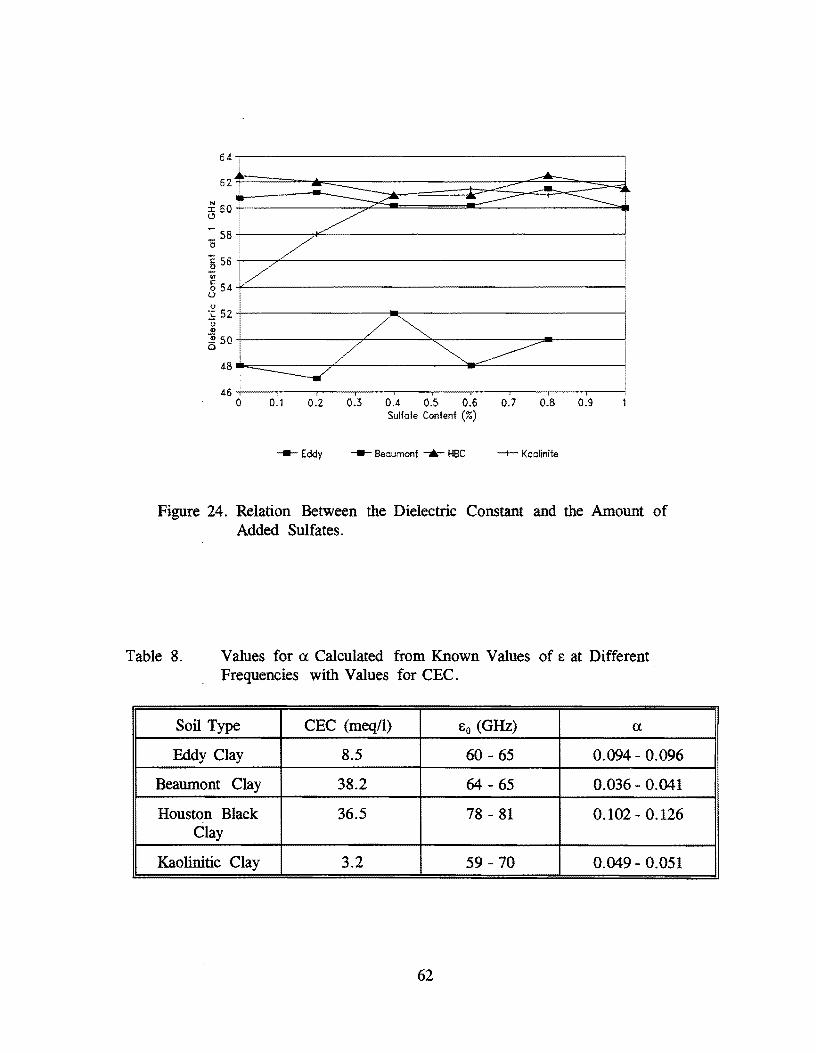
64
62
::: 58 c
§ 56 in g 54 u () :s 52 t.l ., ~ 50
48
46
-= ----....- ~
/ /
/
/~ /
~
...... - --- ---I
I
~ ------ I
o 0.1 0.2 0.3 0.4 0.5 0.6 0.7 0.8 0.9 Sulfate Content (%)
--- Eddy --- Beaumont .....-- HBC -t- Kaolinite
Figure 24. Relation Between the Dielectric Constant and the Amount of Added Sulfates.
Table 8. Values for a. Calculated from Known Values of S at Different Frequencies with Values for CEC.
Soil Type CEC (meq/l) So (GHz) a.
Eddy Clay 8.5 60 - 65 0.094 - 0.096
Beaumont Clay 38.2 64 - 65 0.036 - 0.041
Houston Black 36.5 78 - 81 0.102 - 0.126 Clay
Kaolinitic Clay 3.2 59 -70 0.049 - 0.051
62

The relationships between CEC vs. Eo and CEC vs. a are shown in Figures 25
and 26. In Figure 25, the range of maximum dielectric constant values for the range
of added sulfate contents are plotted against the CEC for each soil type. Three of
these data ranges, the HBC, the Eddy clay, and the kaolinitic clay, seem to plot
within a band, as shown in Figure 25. The Beaumont clay is different from the other
three and does not plot within the same band.
Figure 26 shows how the range of a-values relates to the CEC. Once again, it
can be seen that the data ranges for the kaolinitic clay, the Eddy clay, and the HBC
plots within a band, but the Beaumont clay once again plots on the outside of this
band.
CONCLUSIONS
The CECs for the soils under investigation varied from 0 to 40 meq/lOOg. The
CEC values for the light colored soils seemed to be lower than that for the
dark colored soil; however, this does not always hold true.
The dielectric constant decreases with an increase in frequency for each soil
type. According to Figure 24, the amount of sulfates added to each sample
seemed to have no relation to the dielectric constant of that specific sample.
However, it still remains to be established whether the dielectric constant has
a relation to the natural sulfate content of the soil samples.
The CEC and So seem to be related to each other. Data-ranges for three of
the clay soils fell into a band in which the CEC values increase as 8 0 increases.
The data-range for the Beaumont clay does not fall within this range.
The CEC also seems to be related to ranges of a-values obtained for three of
the soils under investigation. Once again, the Beaumont clay does not conform
to this range.
The . Beaumont clay seems to be the exception in each of the two above
mentioned cases. This phenomenon suggests a difference between the
Beaumont clay and the other three clay soils. However, at this stage, the
difference is still unexplained.
63

40.-------------------------------------------------~
u w
35
30
u 15
10
- Beaumont
Eddy
5 ~~D
I' Kaolinite For pure
O+--______ ir-______ Ti ______ -,i ________ ~------,,~w~a~te~r--~
55 60 65 70 75 80 85 Maximum Dielectric constant (MHz)
Figure 25. Relation between the CEC and the Range of 80 Values.
O. 13 i----------------=::::=====::==_______J
Hou,'oo blod< I 0.12
0.11
0.1
0.09 o to.08 <{
0.07
0.06
Eddy
I
Beaumont' I :::: jl
0.03+-----~----,_----,_----~-----r-----r----_r----~ I I I I I I I I
o 5 10 15 20 25 30 35 40 CEC (Meq/I)
Figure 26. Relation between CEC and Range of a-Values.
64

CHAPTER 7
RESULTS OF LOW CALCIUM FLY -ASH STABILIZATION
INTRODUCTION
Soil often requires stabilization of some sort to enhance mechanical stability.
Pozzolanically induced long-term strength gain is achieved by mixing lime with clay
soils (12). Hydrated lime is one of the most common stabilizers used to enhance
subgrade strength. However, hydrated lime contains high percentages (up to 80%) of
calcium, which sometimes reacts with sulfates present in the soil to form ettringites,
an expandable mineral (1). For this reason, sulfate bearing soils need to be stabilized
with a low calcium stabilizer to prevent ettringite formation. Low calcium fly-ashes
like Sandow, Montecello, and Big Brown have been used to investigate their effects
on sulfate bearing clay soils. The results of expansion tests that were performed with
these low calcium fly-ashes are presented in this chapter. Expansion tests were
performed on the four clay soil samples as well as Sample No. 7 from FM 1382,
which contained the highest amount of natural sulfates and expanded up to 18%
upon lime stabilization (see Figure 13a).
RESULTS OF LOW CALCIUM FLY-ASH STABILIZATION ON FOUR CLAY
SOILS
Each of the clay soils was stabilized with each of the low calcium fly-ashes and
subjected to expansion tests. For each clay. an un-stabilized sample and a sample
stabilized with hydrated lime were also subjected to expansion tests. These samples
served as control samples with which the samples stabilized with low calcium fly-ash
could be compared.
The expansion of Eddy clay samples stabilized with low calcium fly-ashes is
shown in Figure 27(a). The sulfate concentration of the Eddy clay is 0.4 meq!l (1:2
soil:water ratio), which is relatively low and probably will not induce sulfate related
heave. From Figure 27(a), it can be seen that the most effective stabilizer seems to
be hydrated lime. The low calcium fly-ash used to stabilize this clay performed better
than the sample that contained no stabilizer.
65
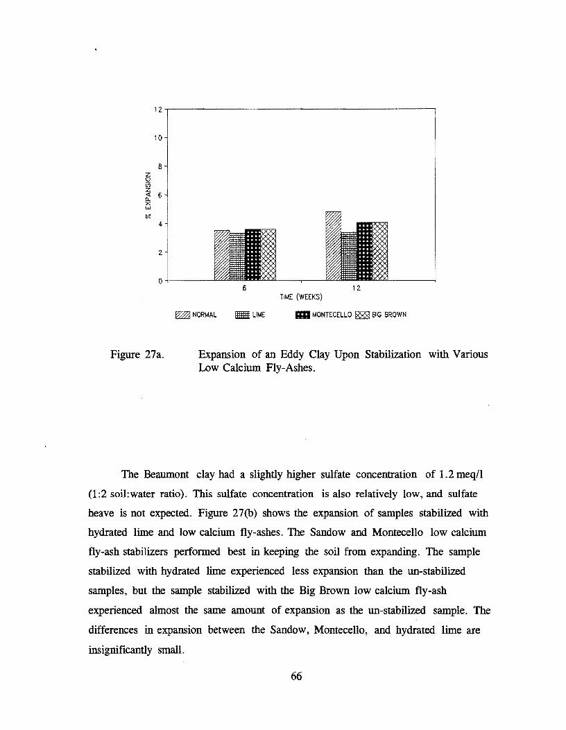
12,----------------------------------------,
z o Vi z
10
8
~ 6 x w ~
4 .
2
o +-____ ----'<LLLL
Figure 27a.
6 12 TIME (WEEKS)
~ NORMAL _ LIME III MONTECELLO BIG BROWN
Expansion of an Eddy Clay Upon Stabilization with Various Low Calcium Fly-Ashes.
The Beaumont clay had a slightly higher sulfate concentration of 1.2 meq/l
(1:2 soil:water ratio). This sulfate concentration is also relatively low, and sulfate
heave is not expected. Figure 27(b) shows the expansion of samples stabilized with
hydrated lime and low calcium fly-ashes. The Sandow and Montecello low calcium
fly-ash stabilizers performed best in keeping the soil from expanding. The sample
stabilized with hydrated lime experienced less expansion than the un-stabilized
samples, but the sample stabilized with the Big Brown low calcium fly-ash
experienced almost the same amount of expansion as the un-stabilized sample. The
differences in expansion between the Sandow, Montecello, and hydrated lime are
insignificantly small.
66

12
10
8 z 0 in z 4 6 0.. X w ti<!
4
2
0
Figure 27b.
6 12 TIME (WEEKS)
~ NORMAL _ LIME l1li SANDOW
~ MONTE CEllO ~ BIG BROWN
Expansion of a Beaumont Clay Upon Stabilization with Various Low Calcium Fly-Ashes.
The Houston black clay had a sulfate concentration of 1.1 meq/l (1:2
soil:water ratio). Despite the relatively low sulfate concentration, the samples
stabilized with low calcium fly-ash seemed to perform better than the sample
stabilized with lime. The expansion of Houston black clay samples is shown in Figure
27(c). Regarding the low calcium fly-ashes, the Big Brown performed worst in
keeping the soil from expanding. However, the difference in expansion between
samples stabilized with low calcium fly-ashes seems to be insignificant.
The kaolinitic clay had the highest sulfate concentration of 12 meq/l
(soil:water ratio of 1:2). This sulfate concentration is relatively high, and sulfate heave
could be expected. The sample that was not stabilized and the sample stabilized with
hydrated lime both expanded more than 8 % after three weeks passed; after that they
came apart, and no further expansion could be monitored. The samples stabilized
with low calcium fly-ashes experienced a maximum expansion of only about 4 % after
12 weeks. This indicates the usefulness of low calcium fly-ashes as stabilizer in sulfate
bearing clay soils.
67
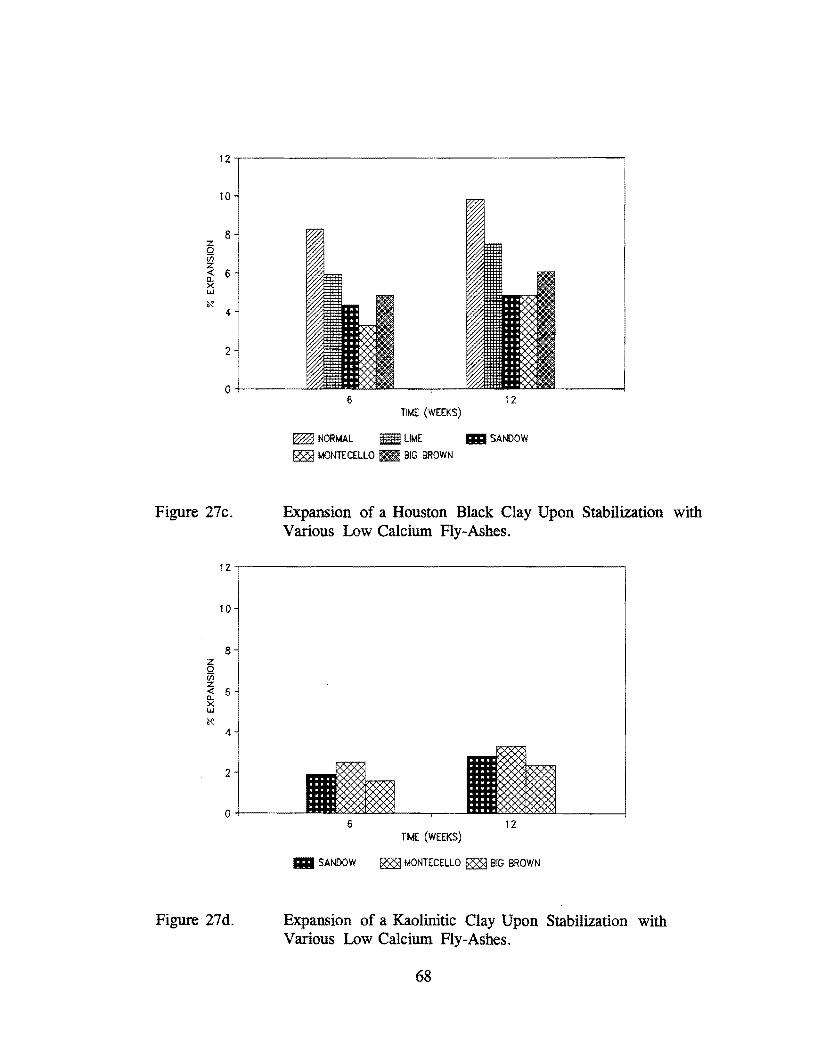
12
10
8 z 0 iii z « 6 0-X W
~ 4
2
0
Figure 27c.
6 12 TIME (WEEKS)
~ NORMAL _ LIME l1li SANDOW
~ MONTE CELLO _ BIG BROWN
Expansion of a Houston Black Clay Upon Stabilization with Various Low Calcium Fly-Ashes.
12~----------------------------------------~
z Q Vl z
10
8
t: 6 x w ~
Figure 27d.
6 12 TIME (WEEKS)
l1li SANDOW ~ MONTE CELLO ~ BIG BROWN
Expansion of a Kaolinitic Clay Upon Stabilization with Various Low Calcium Fly-Ashes.
68

RESULTS OF LOW CALCIUM FLY-ASH STABILIZATION ON FM 1382
SITE NO 7
The sample that experienced the highest amount of expansion upon lime
stabilization was Sample No.7 from FM 1382. Chapter 3 discusses the expansion of
this sample. This sample contained the highest sulfate concentration of all the soils
under investigation, namely, 184.3 meq/l (1:0.5 soi1:water ratio). From Figure 11 (a), it
can be seen that this sample expanded 18% upon lime stabilization after a period of
16 weeks. The sample that was not lime stabilized expanded 14% after 16 weeks. The
expansion of these samples is compared to a sample of the same soil that was
stabilized with Montecello low calcium fly-ash after 6 and 12 weeks. The results are
presented in Figure 28. It is evident that the low calcium fly-ash succeeded in
reducing the amount of expansion encountered after hydrated lime stabilization.
20
18
16
14
a 12 iii z ~ 10 x w ~ 8
6
4
2
0 6 12
TIME (WEEKS)
NORMAL LIME l1li MONTE CELLO
Figure 28. Expansion of Eddy Clay from FM 1382 Site No 7 Upon Stabilization with Montecello Low Calcium Fly-Ash.
69

EV ALUATIONOF DIFFERENT LOW CALCIUM FLY-ASHES AS STABILIZERS
The amounts of expansion of each of the low calcium fly-ash stabilizers were
added together, and an average amount of expansion was calculated for each low
calcium fly-ash stabilizer. This average amount of expansion is plotted against the
calcium concentration of each of the low calcium fly-ashes, and the plot is shown in
Figure 29. The average expansion of all the samples stabilized with hydrated lime is
also shown in Figure 29. The average amount of calcium in hydrated lime is about
80%. The low calcium fly-ashes perfonned better than the hydrated lime in
prohibiting expansion of the clay soils; however, this is only true because of the
relatively high sulfate concentration in some of the soils under investigation. The
small difference in the amount of calcium between the different low calcium fly ash
stabilizers does not seem to have much relation to the amount of expansion. It is,
however, evident that the Big Brown did not perfonn as well as the other two
stabilizers.
6
~5 "--' Brown c 0 'iii § 4 0. x Montecello w
Sandow
""" o 3 i: :l 0 E
<I: 2 <l) (1) 0 '-<l)
~1
0 8.47 9.8 13 80
Calcium Content (%)
Figure 29. The Average Amount of Expansion for Each Stabilizer vs. the Calcium Content of the Stabilizer.
70

CONCLUSIONS
Soils with a relatively low sulfate content like the Eddy clay, the Houston
black clay, and the Beaumont clay performed well after stabilization with
hydrated lime and low calcium fly-ash.
When the sulfate concentration is relatively low, hydrated lime could be used
with as much success as low calcium fly-ashes.
For low sulfate concentrations, the difference between expansion of low
calcium fly-ash and hydrated lime stabilized samples seems insignificant.
With relatively high sulfate concentrations, hydrated lime does not seem to
reduce the expansion of clay soils. In some cases, the addition of hydrated lime
is even more deleterious than no stabilization at all. However, low calcium fly
ash seems to minimize the amount of expansion that occurs.
From Figure 28, it is evident that the overall average expansion of samples
stabilized with low calcium fly-ashes is lower than the overall average
expansion of samples stabilized with hydrated lime. However, this seems to be
true only when considering soils with relatively high sulfate contents. A small
difference in calcium content seems not to have any relation to the amount of
expansion encountered. However, the Big Brown did not perform as well as
the other two low calcium fly-ash stabilizers.
It is suggested that low calcium fly-ashes be used with relatively high sulfate
concentrations, while hydrated lime could be used when sulfate concentrations
are relatively low.
71


CHAPTERS
INTERACTIVE DISCUSSION OF ALL RESULTS
INTRODUCTION
The results obtained from expansion tests and electrical conductivity tests on
samples containing different amounts of sulfates were presented in Chapters 3 and 4,
respectively. The results of CEC and dielectric constant determination were presented in
Chapter 5, and the results of low calcium fly-ash stabilization were presented in Chapter 6.
All of these results were discussed individually at the end of each chapter.
It is now necessary to investigate possible interactions between the results obtained
in the last four chapters. A statistical regression model has been used to determine
interaction between expansion, electrical conductivity (EC), sulfate content, CEC, and
dielectric constant (DC) of the various soil samples under investigation. The results of this
statistical model will be presented and discussed in this chapter.
The results can be divided into four groups. Two of the groups use the percentage
of expansion of soil samples without the addition of lime as a response variable. The first
group is composed of the four clay soil samples, and the other constitutes the samples
obtained from IH 45 and FM 1382.
The other two groups use the percentage of expansion of soil samples with the
addition of 6% hydrated lime as a response variable. Once again, the four clay soil
samples are modeled separately from samples obtained from IH 45 and FM 1382. The
reason for this is the sulfate content determination at different soil:water ratios which
cannot be compared.
MODEL 1: REGRESSION MODELING WITH % EXPANSION WITHOUT LIME
AS RESPONSE VARIABLE FOR THE FOUR CLAY SOIL SAMPLES
The results from different experimental procedures that were used to perform a
regression analysis are presented in Table 9.
73

Table 9. Results of Various Experimental Procedures for the Four Clay Soil Samples (Without Lime).
Soil Type % Expansion Sulfate Content CEC EC DC (No Lime) (meqll) (meq/100g) (mS/cm)
Eddy clay 3.28 0.4 8.5 0.295 48
Beaumont 6.72 1.2 38.2 0.510 60.8 clay
HBC 8.44 1.1 36.5 0.760 62.5
Kaolinitic 15.00 12 3.2 0.601 54.2 clay
All of the results reported are from soil samples containing no lime and no added
sulfates. The amounts of expansion of the samples are reported after 6 weeks of exposure
to cold and humid conditions. After 6 weeks, the kaolinitic clay had fallen apart, and
expansion could not be monitored. However, a conservative calculated guess has been
made regarding the expansion of the kaolinitic clay in order to be able to perform a
regression analysis on the data.
where
The following equation describes the proposed full model:
Exlime = 80 + 8,Sulf + 82CEC + 8)EC + B4DC
Exnolime = % Expansion of soil samples without addition of lime
Sulf = Sulfate content (meq/l)
CEC = Cation Exchange Capacity (Meq/IOOg)
EC = Electrical Conductivity (mS/cm)
DC Dielectric Constant (GHz)
Because the number of parameters do not exceed the rank, the least-squares solutions for
the parameters are not unique and, therefore, some statistics will be misleading (20). The
parameter estimates for the full model are biased, and the full model had to be rejected. It
74

was, however, possible to obtain Pearson Correlation Coefficients for all the parameters
(20). Table 10 presents correlation coefficients.
Table 10.
Exnolime
Sulf
CEC
EC
DC
Pearson Correlation Coefficients for Expansion of Clay Soil Samples Containing No Lime, and Other Parameters (19).
Exnolime Sulf CEC EC DC
1.000 0.923 -0.302 0.603 0.218
0.923 1.000 -0.620 0.258 -0.157
-0.302 -0.620 1.000 0.452 0.862
0.603 0.258 0.452 1.000 0.809
0.218 -0.157 0.862 0.809 1.000
Parameters that are highly correlated with the amount of expansion are the sulfate
content and the electrical conductivity with correlation coefficients of 0.923 and 0.603,
respectively. Other parameters that are correlated with each other are the dielectric
constant with CEC and electrical conductivity. However, since these parameters do not
seem to correlate with the amount of expansion, they could be omitted. The following
reduced model is proposed:
Exnolime = 130 + 131 Sulf + 132EC
This model does not have the same problem as the full model since the number of
parameters is greater than the rank of the model. The parameter estimates for the reduced
model as produced by the SAS-program output are as follows:
130 = 0.000
B) = 1.071
132 = 1.071
75

MODEL 2: REGRESSION MODELING WITH % EXPANSION WITH 6% LIME
AS RESPONSE VARIABLE FOR THE FOUR CLAY SOIL SAMPLES
" Table 11 contains the data used to perfonn a regression analysis on the four clay
soil samples with the amount of expansion after lime stabilization as the response variable.
The analysis was perfonned in exactly the same way as described in the previous section.
Again, the full model was rejected. The Pearson correlation coefficients are presented in
Table 12. The correlation coefficients vary only with insignificant small amounts from
those in the previous section. Because of the similarity in the two models, the same
reduced model is proposed with exactly the same parameter estimates.
Table 11. Results of Various Experimental Procedures for the Four Clay Soil Samples (With Lime).
Soil Type % Expansion Sulfate CEC EC DC (6% Lime) Content (meqIlOOg) (mS/cm) (GHz)
(meqll)
Eddy clay 2.969 0.4 8.5 0.295 48
Beaumont 7.813 1.2 38.2 0.510 60.8 clay
HBC 6.563 1.1 36.5 0.760 62.5
Kaolinitic 15.00 12 3.2 0.601 54 clay
Table 12. Pearson Correlation Coefficients for Expansion of Clay Soil Samples Containing 6% Lime, and Other Parameters (19).
Exlime Sulf CEC EC DC
Exlime 1.000 0.938 -0.315 0.463 0.172
Sulf 0.937 1.000 -0.620 0.258 -0.157
CEC -0.315 -0.620 1.000 0.452 0.862
EC 0.463 0.258 0.452 1.000 0.809
DC 0.172 -0.157 0.862 0.809 1.000
76
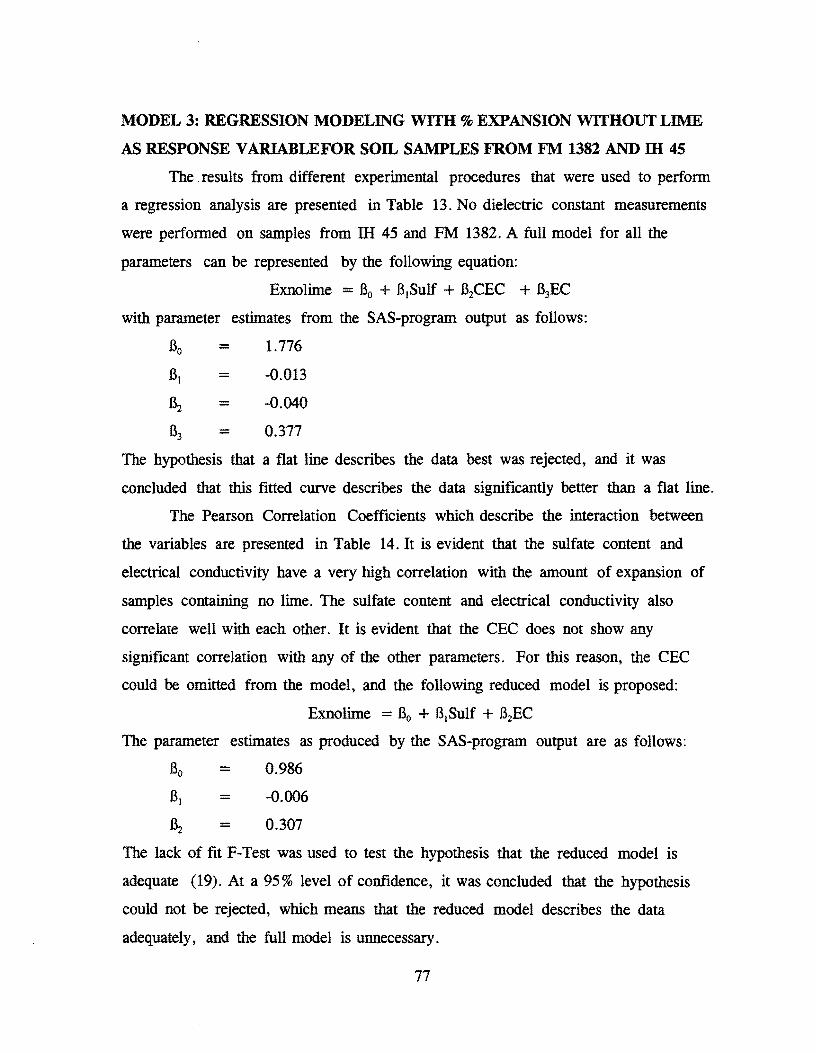
MODEL 3: REGRESSION MODELING WITH % EXPANSION WITHOUT LIME
AS RESPONSE V ARlABLEFOR SOIL SAMPLES FROM FM 1382 AND m 45
The results from different experimental procedures that were used to perform
a regression analysis are presented in Table 13. No dielectric constant measurements
were performed on samples from IH 45 and FM 1382. A full model for all the
parameters can be represented by the following equation:
Exnolime = Bo + B]Sulf + B2CEC + B3EC
with parameter estimates from the SAS-program output as follows:
Bo = 1.776
B] = -0.013
B2 = -0.040
B3 - 0.377
The hypothesis that a flat line describes the data best was rejected, and it was
concluded that this fitted curve describes the data significantly better than a flat line.
The Pearson Correlation Coefficients which describe the interaction between
the variables are presented in Table 14. It is evident that the sulfate content and
electrical conductivity have a very high correlation with the amount of expansion of
samples containing no lime. The sulfate content and electrical conductivity also
correlate well with each other. It is evident that the CEC does not show any
significant correlation with any of the other parameters. For this reason, the CEC
could be omitted from the model, and the following reduced model is proposed:
Exnolime = Bo + B1Suif + B2EC
The parameter estimates as produced by the SAS-program output are as follows:
Bo - 0.986
=
=
-0.006
0.307
The lack of fit F-Test was used to test the hypothesis that the reduced model is
adequate (19). At a 95% level of confidence, it was concluded that the hypothesis
could not be rejected, which means that the reduced model describes the data
adequately, and the full model is unnecessary.
77

Table 13. Results of Various Experimental Procedures for Soil Samples from FM 1382 and IH 45 (Without Lime).
Soil Number % Expansion Sulfate CEC EC (No lime) Content (Meq/100g) (mS/cm)
i
(Meq/l)
IH 45 1.875 0.7 26.6 2.7 1
2 3.380 0.5 30.4 2.5
3 1.860 0.5 31.2 2.5
4 1.570 0.7 9.2 1.9
6 0.620 1.3 16.7 2.0
8 0.310 0.6 16.3 1.9
9 1.24 0.5 37.5 2.3
FM 1382 6.27 45.5 14.3 4.3 1
2 1.56 3.5 19.3 2.4
3 0.31 0.4 10.6 1.6
5 0.94 5.6 35.6 2.7
7 8.62 184.3 35.6 27.7
Table 14. Pearson Correlation Coefficients for Expansion of Soil Samples from FM 1382 and IH 45 Containing No Lime. and Other Parameters (19).
Exnolime SuIf CEC EC
Exnolime 1.000 0.713 0.163 0.755
Sulf 0.713 1.000 0.279 0.959
CEC 0.163 0.279 1.000 0.369
EC 0.755 0.959 0.369 1.000
78

MODEL 4: REGRESSION MODELING WITH % EXPANSION WITH 6% LIME
AS RESPONSE V ARIABLEFOR SOn.. SAMPLES FROM FM 1382 AND IH 45
The results from different experimental procedures that were used to perfonn
a regression analysis are presented in Table 15. The hypothesis that a flat line
described the data best was rejected, and the full model that describes the curvature
in data is presented by the following equation:
Exlime = Bo + B1Suif + B2CEC + B3EC
with parameter estimates from the SAS-program output as follows:
Bo = -0.408
=
=
0.000
-0.013
0.512
From Table 16, it is evident that the amount of expansion of the samples
containing 6 % lime correlates relatively well with the sulfate content and the
electrical conductivity of the samples. On the other hand, the correlation between the
electrical conductivity and the sulfate content of the samples is very high. Since the
CEC does not seem to relate well to any of the other parameters, it could be omitted
from the model, and a reduced model could be fitted to the data. The reduced model
can be represented by the equation:
Exlime = Bo + B1Sulf + ~EC The parameter estimates as produced by the SAS-program output are as follows:
Bo = -0.670
0.002
0.448
The lack of fit F-Test was once again used to detennine that the reduced model is
adequate and that the full model is not needed (19).
79

Table 15. Results of Various Experimental Procedures for Soil Samples from FM 1382 and IH 45 (With Lime).
Soil Number % Expansion Sulfate CEC EC (6% lime) Content (Meq/l00g) (mS/em)
(Meqll)
IH 45 0.23 0.7 26.6 2.7 1
2 0.15 0.5 30.4 2.5
3 0.94 0.5 31.2 2.5
4 0.31 0.7 9.2 1.9
6 0.00 1.3 16.7 2.0
8 0.31 0.6 16.3 1.9
9 0.31 0.5 37.5 2.3
FM 1382 0.56 45.5 14.3 4.3 1
2 0.63 3.5 19.3 2.4
3 0.63 0.4 10.6 1.6
5 4 5.6 35.6 2.7
7 13.31 184.3 35.6 27.7
Table 16. Pearson Correlation Coefficients for Expansion of Soil Samples from FM 1382 and IH 45 Containing 6% Lime, and Other Parameters (19).
Exlime SuIf CEC EC
Exlime 1.000 0.959 0.320 0.997
Sulf 0.959 1.000 0.254 0.959
CEC 0.320 0.254 1.000 0.351
EC 0.997 0.959 0.351 1.000
80

MODEL FOR DETERMINATION OF AMOUNT OF EXPANSION EXPERIENCED
BY SULFATE BEARING CLAY SOILS
In each of the four regression analyses perfonned in this chapter, the data
were best described by a model containing only expansion, electrical conductivity, and
natural sulfate content of the soil samples as parameters. From the correlation
coefficients obtained for each model as well as from the regression equations
obtained in Chapter 4, it can be seen that electrical conductivity relates well to
sulfate content. The regression models from Chapter 4 were as follows:
a) For soil samples from FM 1382 and IH 45 with a soil:water ratio of
1:20
EC = exp{0.799 + 0.014(sulfate content)}
b) For the four clay soil samples with a soil:water ratio of 1:2
EC = 5.785(sulfate content) + 0.623
Electrical conductivity of soil can be measured with a permittivity probe on in
situ soil in the field with great ease. Depending on the soil:water ratio used to make
a soil paste on which electrical conductivity is measured, one of the above equations
could be used to estimate the amount of sulfates present in the soil.
Once the amount of sulfates and the electrical conductivity are known, the
suitable regression model from this chapter could be used to detennine an estimated
amount of expansion. If this amount exceeds the maximum allowable amount of
expansion, low calcium fly-ash should be used to stabilize the soil, rather than
hydrated lime.
Because the amount of sulfates is a function of the electrical conductivity, the
equations obtained in Chapter 4 could be substituted into each model, and the
regression equations could be written in the following way:
Model 1:
Exnolime = 1.255(EC) - 0.11526
81

Model 2:
Exlime = L255(EC) - 0.11526
Model 3:
Exnolime = 1.328 - 0.429Ln(EC) + 0.307(EC)
Model 4:
Exlime = 0.43Ln(EC) + 0.488(EC) - 0.784
Models 1 and 2 are the same and should be used when the soil:water ratio of
the paste from which the electrical conductivity was measured is 1:2. Models 3 and 4
should be used if electrical conductivity was measured on a soil paste with a
soil:water ratio of 1 :20.
Since it is anticipated that soil with a high sulfate content should expand more
upon lime stabilization, it does not make sense to use the same model for predicting
expansion with and without lime stabilization. The reason models 1 and 2 are the
same is probably because none of the four clay soils used in predicting these models
contained substantially high amounts of natural sulfates to cause ettringite formation.
In contrast to models 3 and 4, the expansion of soils in models 1 and 2 was probably
not sulfate related. It is proposed that models 3 and 4 be used to predict expansion of
soils before and after lime stabilization, respectively.
CONCLUSIONS
Four regression models were suggested which relate the results from different
experimental procedures to each other. Each of full models contained
electrical conductivity, CEC, dielectric constant, and the amount of soluble
sulfates as parameters with the amount of expansion with or without lime as a
response variable.
In each case, a reduced model has been proposed and accepted. For each of
the models, the reduced model had only sulfate content and electrical
conductivity as parameters.
82

Model 1 and 2 are exactly the same, which means the amount of expansion
before and after lime stabilization would be equivalent. This does not make
sense since the amount of expansion should be less after lime stabilization of
soils that do not contain sulfates, and if the stated hypothesis holds true, the
amount of expansion after lime stabilization should be higher upon
stabilization of sulfate bearing soils. Thus, models 1 and 2 should not be used.
None of the four clay soils used in the experimentation to obtain models 1 and
2 contained high amounts of natural sulfates. The kaolinitic clay contained the
highest amount of sulfates which was 0.06%. The relatively high amount of
expansion experienced by this clay soil was probably due to its high plasticity
and surface area and was not sulfate related.
Models 3 and 4 were obtained from experimental data on soils from FM 1382
and IH 45. Natural sulfate contents of up to 0.9% were encountered in some
of the soil samples. Model 3 provides an equation for the calculation of
expansion of soil samples that is not lime stabilized. Model 4 provides a
similar equation for expansion of soil samples that have been stabilized with
6% of hydrated lime.
Models 3 and 4 may be used to calculate the amount of expansion as a
function of the electrical conductivity as measured by the permittivity probe on
a soil paste with 1 :20 soil:water ratio.
83

OVERALL CONCLUSIONS
CHAPTER 9
CONCLUSION
In order to view the conclusions in their proper perspective, it will be useful to
review the questions that were posed at the beginning of this investigation. These
questions can be summarized as follows:
Do sulfate bearing soils pose a problem when stabilized with lime?
Can those soils that are susceptible to sulfate induced heave be identified?
Is there a field-test procedure that can be used to predict the amount of
expansion likely to occur?
If lime stabilization causes sulfate induced heave in clay soils, what alternative
method of stabilization can be used?
Proposed answers for these questions are:
Mitchell (14) concluded that when sulfates are present in soil they could cause
excessive heave in clay soils that have been stabilized with lime due to the
formation of ettringite. In Chapter 3, it was shown that soils containing
relatively high sulfate contents expanded more upon lime stabilization than
soils not containing sulfates.
The electrical conductivity of the soils under investigation relates well to the
sulfate content in the soils and can be used to determine whether soil contains
sulfates or not. Regression models that relate electrical conductivity to sulfate
content were developed in Chapter 4.
A permittivity probe can be used to measure electrical conductivity and
dielectric constants of soil samples. In Chapter 7, a model was proposed that
can predict the amount of expansion if the electrical conductivity and sulfate
content of the soil are known. Since electrical conductivity could be measured
in the field with a permittivity probe, and the sulfate content in soils is a
function of electrical conductivity, both parameters are known and can be
85

substituted into equations that yield the amount of expansion with and without
lime stabilization.
It has been concluded that lime stabilization of sulfate bearing soils causes
ettringite fonnation which leads to excessive heave. Chapter 6 proposes that
low calcium fly-ash, like Sandow, Montecello, or Big Brown be used to
stabilize clay soils that are likely to expand beyond acceptable levels. This
expansion can typically be predicted with the model that was proposed in
Chapter 7 .
. SUBJECTS PROPOSED FOR FURTHER INVESTIGATION
Only five soil properties were taken into account in this investigation. These
properties are the amount of expansion, sulfate content, dielectric constant, cation
exchange capacity, and electrical conductivity. Amongst these five properties, only
sulfate content, electrical conductivity, and the amount of expansion had relatively
good interaction with each other. There are numerous other soil properties that could
be investigated. Two of these are the surface area and gradation of the soil which
could easily be measured with modem laser technology. It could also be
advantageous to have a full account of the mineralogical composition of the soil
under investigation. However, it would not be possible to detennine the .mineralogical
composition of in situ soil in the field with ease.
The equations developed to detennine amounts of expansion of soil with and
without lime stabilization are empirical. About 15 different soil samples were used to
develop the relationships presented in this investigation. These soils all originated
from Texas and, therefore, it is suggested that the equations should only be used for
detennining expansion of soil samples from the same geological fonnations. Similar
equations could, however, be developed for other soil fonnations.
A characteristic of the soil in Texas is that sulfates seem to be the only salt
that occurs in the top horizons of soil fonnation. This may be because sulfate is one
of the most insoluble salts. All other salts are washed down to the maximum depth of
penetration. For this reason, electrical conductivity relates well to the sulfate content
86

of soils. However, in areas with very low precipitation, other salts could be present in
the top horizons and would have an influence on the electrical conductivity. The
effect this will have on the prediction of sulfates in soil needs to be investigated.
Water leaching through sulfate bearing soils is believed to dissolve the sulfates
in the soil and make the sulfates more available for reaction with calcium, to form
ettringites. Isolating the sulfate bearing clay soils from moisture activity would lead to
drastic reduction in sulfate related expansion. Vertical and horizontal moisture
barriers proved to be effective in controlling moisture activity of soils underneath
pavements (21). Although it is evident that moisture barriers reduce roughness
wavelengths associated with expansive soils, it is now necessary to investigate the
effectiveness of moisture barriers used in association with sulfate bearing clay soils.
87


CHAPTER 10
IMPLE:MENTATIONOF RESULTS
By using the models developed in chapter 8 of this report, it should now be
possible to predict whether sulfate swell is probable to occur in clay soils and also the
amount of sulfate related swell that could be expected.
The equipment needed to perfonn a field evaluation of the sulfate content in
soils includes the following:
a) Wide mouth plastic containers with water-proof lids,
b) Distilled water,
c) Battery driven digital scale that can measure up to 500 g (Figure 30),
d) Hand held conductivity meter (Figure 31), and
e) Calibration solutions for the conductivity meter.
The entire package costs less than $600.
The procedure is as follows:
Step 1: Find the location where the sulfate test is to be perfonned and use an
auger to obtain two small soil samples at approximately 10 and 20 cm
below the soil surface. Only 5 grams of soil is needed to perform the
test.
Step 2:
Step 3:
Step 4:
Weigh approximately 5 g of each soil sample into two separate plastic
containers. If the soil is wet, break lumps apart and leave the soil to
air-dry for 1 to 2 hours. Record the exact dry weight of the samples.
Now add distilled water with a mass of exactly 20 times the dry weight
of the soil sample to the dry sample. Tightly close the lid of the plastic
container and shake vigorously until the soil dissolves and forms a
homogeneous solution.
Calibrate the conductivity meter as described in the instruction manual
accompanying the device.
89

Step 5:
Step 6:
Take conductivity measurements on each soil:water mixture and record
the data in milli Siemens (mS)
Note: 1 uS = 0.001 mS
From our limited experience, mixtures with a conductivity of more than
8 mS have a potential to cause problems.
Use the following equation to determine an estimated amount of
expansion that would occur upon lime stabilization:
% Expansion = 0.43Ln(EC) + 0.488(EC) - 0.784
where EC = Electrical Conductivity measurement in mS, and %
Expansion = Anticipated swell after curing in moist environment for 7
days.
91


REFERENCES
1. T.M. Petry and D.N. Little. Update on Sulfate-Induced Heave in Treated
Clays; Problematic Sulfate Levels. Transportation Research Record 1362, TRB,
National Research Council, Washington, DC, pp. 51 - 55.
2. G.A. Ferris, J.L. Eades, R.E. Graves, and G.H. McClellan. Improved
Characteristics in Sulfate Soils Treated with Barium Compounds Before Lime
Stabilization. Transportation Research Record 1295, TRB, National Research
Council, Washington, DC, pp. 45 - 51.
3. D. Hunter. Lime-Induced Heave in Sulfate-Bearing Clay Soils. Journal of
Geotechnical Engineering 22168. Vol. 114, No.2, February 1988, pp. 150 - 167.
4. L.A. Richards, L.E. Allison, L. Bernstein, C.A. Bower, J.W. Brown et al.
Diagnosis and Improvement of Saline and Alkali soils. Agriculture Handbook
No. 60, United States Department of Agriculture. U.S. Government Printing
Office, Washington, DC, February 1954.
5. J.D. Rhoades and A.D. Halvorson. Electrical Conductivity Methods for Detecting
and Delineating Saline Seeps and Measuring Salinity in Northern Great Plains
Soils. Agriculture Research Service W-42. United States Department of
Agriculture, March 1977. (Available in Texas A&M University Library,
Documents Division)
6. 1. Shainberg and J. Shalhevet. Soil Salinity under Irrigation Processes and
Management. Ecological Studies Vol. 51. Springer-Verlag, New York, 1984.
7. T. Plakk. HF Permittivity Measurements by Capacitive Probe. Adek LTD Uus
Saku 12-1. Saku EE34oo, Estonia. (personal collection of Sanet Bredenkamp)
8. M. Whitney and L.J. Briggs. An Electrical Method of Determining the
Temperature of Soils. U.S. Department of Agriculture, Division Soils Bulletin 7,
15 pp.
93
9. Soil Survey of Dallas County, Texas. United States Department of Agriculture
Soil Conservation Service in Cooperation with Texas Agricultural Experiment
Station. February 1980. (Available in TTl Library, Texas A&M University,
Civil Engineering Department, Materials Division, CE\ TTl Building)
10. I.B. Dixon and S.B. Weed. Minerals in Soil Environments. SSSA Book Series
No. 1. Published by Soil Science Society of America, Madison, WI, 1989.
11. S. Bredenkamp and J.B. Dixon. Analysis of an Eddy Clay. Final report for
AGRO 626. Texas A&M University, College Station, December 1993.
12. V.C. Farmer and I.D. RusseL Interlayer Complexes in Layer Silicates. The
Structure of Water in Lamellar Ionic Solutions. Trans Faraday Society Vol. 67,
No. 2737, pp. 345 - 365, 1971. (Personal collection of Dr. J.B. Dixon, Texas
A&M University, Agronomy Department).
13. Handbook for Stabilization of Pavement Subgrades and Base Courses with Lime.
National Lime Association, December 1993. (personal collection of Dr. Dallas
N. Little, Texas A&M University, Civil Engineering Department).
14. K. Mitchell. Practical Problems from Surprising Soil Behavior. (The Twentieth
Karl Terzaghi Lecture). Journal of Geotechnical Engineering. Vol. 112, No.3,
March 1986, pp. 259 - 289.
15. R.D. Holtz and W.D. Kovacs. An Introduction to Geotechnical Engineering.
Prentice-Hall, Englewood Cliffs, NJ, 1989.
16. EPA Method No 9050. Specific Conductance. Soil Analytical Services Inc.
College Station, TX, Revised, September 1986.
17. EPA Method No 9081. Cation Exchange Capacity of Soils. Soil Analytical
Services Inc. Revised, September 1986.
18. EPA Method No 9038. Soluble Sulfates (Turbidimetric). Soil Analytical Services
Inc. Revised, September 1986.
19. I.S. Milton and J.C. Arnold. Introduction to Probability and Statistics: Principles
and Application for Engineering and the Computing Sciences. McGraw-Hill
Publishing Company, 1990.
94

20. EPA Method No 9040. PH Electrometric Measurement. Soil Analytical Services
Inc. Revised, September 1986.
21. F.N. Nyangaga, R.L. Lytton and D.A. Gay. Effects of vertical moisture barriers
on roughness development of pavements on expansive soils. First International
Conference on Unsaturated Soils. Paris, 1995.
95


APPENDIX A
97


., . i , i
') '. ,
Locations from which Soil Samples Were Taken Along FM 1382
99

, , , , , , , , , , , , , , +', ,
" " , , +, , ,
" , , , ,
Locations from which Soil Samples Were Taken Along III 45
100
+ +

APPENDIXB
101


RELATION BETWEEN PH OF CLAYSOn.s AND AMOUNT OF EXPANSION
ENCOUNTERED
One of the tasks of this report was to investigate the effect of high pH liquids
on the expansion of sulfate bearing clay soils. The pH of each of the soil samples
from IH 45 and FM 1382 was measured using EPA-method No. 9040 (20). The pH of
a sample is determined electrometrically using either a glass electrode in combination
with a reference potential or a combination electrode (20). The pH values for these
clay soil samples varied between a pH of 7.8 and 9.2. Figure 32 shows the relation
between the pH of each sample to the amount of expansion encountered after lime
stabilization. From this figure it is clear that there is no apparent relationship
between the amount of expansion that occurs after lime stabilization and the pH of
the clay soil.
14 •
12
10 ,..... ~ '-'
c 8 0
"iii c c 6 0.. X w
4 •
2 • • • • 0 • • • • 7.8 8 8.2 8.4 8.6 8.8 9 9.2
pH of Clay Soils
Figure 32. Relation Between pH of Clay Soils and the Amount of Expansion After Lime Stabilization.
103

This phenomena validated the decision to abandon all further research
concerning raising the pH of the sulfate bearing clay soil samples. Another reason for
abandoning this investigation was because of the high cost involved in entering the
high pH liquids into the low permeability clay soils.
104


