

Reliability/Availability of Manufacturing Cells and Transfer Lines
by
Balaji Kannan
A thesis submitted to the Graduate Faculty of Auburn University
in partial fulfillment of the requirements for the Degree of
Master of Science
Auburn, Alabama May 9, 2011
Keywords: Reliability, Availability, Manufacturing cells, Transfer Lines, Maximum likelihood estimation
Approved by
JT. Black, Co-chair, Professor Emeritus of Industrial & Systems Engineering Saeed Maghsoodloo, Co-chair, Professor Emeritus of Industrial & Systems Engineering
Amit Mitra, Professor of Management

ii
Thesis Abstract
One of the major wastes in a manufacturing system is downtime caused by machine
breakdown/failure and the time and cost incurred to repair the failed machine. Machine
breakdown leads to stoppage of production in manufacturing cells and automated serial
production lines (Transfer lines) until the machine is brought back to operable condition.
Obtaining the reliability/availability measures of machines in manufacturing systems is
necessary to schedule preventive maintenance and periodic replacement of critical components
in order to increase manufacturing uptime. To assess the reliability measures and availability of
manufacturing cells and transfer lines, field failure data were collected from a crankshaft
manufacturing cell and an automated transfer line and were fitted to relevant statistical
distributions using Goodness of fit tests, and the necessary reliability and availability measures
were obtained using Maximum likelihood estimation (MLE). The results were that the time
between failures of CNC machines and Transfer Lines follows the Weibull distribution (in most
cases) and Transfer Lines require higher maintenance requirements than manufacturing cells.
iii
Table of Contents
Abstract…………………………………………………………………………………………...ii
List of Tables……………………………………………………………………………………...v
List of Figures………………………………………………………………………………….....vi
List of Notation and Acronyms……………………………………………...…………………..vii
1.0 Introduction …………………………………………………………………………………...1
2.0 Literature Review …………………………………………………………………………......4
3.0 Manufacturing Cells and Transfer Lines – A concise overview……………………………..17
3.1 Manufacturing Cells……………………………………………………………………...17
3.2 Transfer Lines …………………………………………………………………………...21
4.0 Reliability in Manufacturing systems design ………………………………………………..23
5.0 Reliability/Availability assessment of Manufacturing Cell………………………………….26
5.1 Identifying appropriate TBF distribution for individual machine tools in crankshaft manufacturing cell……………………………………………………………………….34
5.1.1 CNC Lathe…………………………………………………………………………34
5.1.2 CNC Mill…………………………………………………………………………..39
5.1.3 CNC Drilling & Boring machine ………………………………………………….42
5.1.4 CNC Grinding machine……………………………………………………………43
5.2 Reliability measures for the machine tools in the manufacturing cell…………………...47
5.2.1 CNC Lathe…………………………………………………………………………49
5.2.2 CNC Mill…………………………………………………………………………..50
iv
5.2.3 CNC Drilling & Boring machine…………………………………………………..52
5.2.4 CNC Grinding machine……………………………………………………………52
5.3 Manufacturing cell reliability estimation…………………………………………………..54
5.4 Manufacturing Cell Availability Estimation……………………………………………….55
5.5 Reliability Estimation – Sensitivity Analysis ……………………………………………..56
6.0 Reliability Availability assessment of Transfer line…………………………………………58
6.1 Identifying appropriate time between failures (TBF) distribution for the Transfer line…...63
6.1.1 Case 1: The TBF has a Weibull distribution (Removing only the Extreme outliers)..70
6 .1.2 Case 2: The TBF is exponentially distributed (Removing both mild and extreme outliers……………………………………………………………………………….72
6.2 Identifying appropriate time to repair (TTR) distribution for the Transfer line…………...74
6.3 Estimating Reliability of the Transfer Line………………………………………………..82
6.3.1 Case 1: Using Weibull TBF Distribution…………………………………………….82
6.3.2 Case 2: Using Exponential TBF distribution ………………………………………..84
7.0 Results …………………………………………………………………………………….....86
8.0 Conclusion …………………………………………………………………………………..88
References ……………………………………………………………………………………….90
Appendix ………………………………………………………………………………………...94

v
List of Tables
Table 3.1: Lean Tools and Manufacturing waste………………………………………………...19
Table 5.1: Time between failures of CNC lathe………………………………………………....30
Table 5.2: Time between failures for CNC Milling machine……………………………………31
Table 5.3: Time between failures for CNC Drilling/Boring machine …………………………..32
Table 5.4: Time between failures of CNC Grinding machine …………………………………..33
Table 5.5: Minitab Goodness of test results for CNC Lathe TBF……………………………….34
Table 5.6: Minitab Goodness of test results for CNC Milling machine TBF ………………...…39
Table 5.7: Minitab Goodness of test results for CNC Drilling & Boring machine TBF………...42
Table 5.8: Minitab Goodness of test results for CNC Grinding machine TBF …………………43
Table 5.9: Distribution parameter(s) estimates for the machine tools in the manufacturing cell..46
Table 5.10: Manufacturing cell reliability estimation – Sensitivity analysis ……………………57
Table 6.1: Time between failures and time to repair of a 15 station palletized Transfer line …..60
Table 6.2: Minitab Goodness of fit tests for transfer line TBF ………………………………….64
Table 6.3: Minitab Descriptive Statistics for Transfer Line TBF ……………………………….65
Table 6.4: Minitab Goodness of fit tests after removing extreme outliers ……………………...68
Table 6.5: Minitab Goodness of fit tests after removing both mild and extreme outliers……….69
Table 6.6: Minitab Goodness of fit tests for Transfer line TTR after removing extreme outliers………………………………………………………………………………...74
Table 6.7: Minitab Goodness of fit tests for Transfer line TTR after removing mild and extreme outliers………………………………………………………………………………...78
vi
List of Figures
Figure 5.1: Crankshaft manufacturing cell………………………………………………………27
Figure 6.1: A 15 station palletized Transfer line………………………………………………...58
Figure 6.2: Minitab Boxplot for Transfer line TBF……………………………………………...66
Figure 6.3: Modified Minitab Boxplot for Transfer line TBF…………………………………...67
Figure 6.4: Minitab Boxplot for transfer line TTR……………………………………………....76
Figure 6.5: Modified Minitab Boxplot for transfer line TTR…………………………………....77

vii
List of Notations and Acronyms
t – Mission time
T – Time between failures
f(t) – Failure density function of T at time t
F(t) =Q(t) = Cumulative density function (cdf) of T or cumulative failure probability by time t
or the unreliability function by time t
Ri(t) – Reliability of the ith component/machine tool
RSYS(t) – Reliability of the system/ Manufacturing cell
hi(t) – Failure rate/ hazard function of the ith component/ machine tool
hsys(t) – Hazard function of the system/ manufacturing cell
Hi(t) – Cumulative hazard function of the ith machine tool
Hsys(t) – Cumulative hazard function of the system/ manufacturing cell
TBF – Time between failures
MTBFi – Mean time between failures of the ith machine tool
MTBFsys – Mean time between failures of the system/manufacturing cell
MLE – Maximum likelihood estimate
WIP – Work In Process Inventory
CNC – Computer Numerical Control

1
CHAPTER 1
Introduction
Reliability is one of the most important characteristics of components, products, and large
complex systems. Manufacturing can be defined as the process of converting materials from one
form to the form that customer’s desire. Products are manufactured according to customer or
design specifications. Quality of a manufacturing company can be measured by the organizations
ability to produce defect-free, reliable components or products. Defect is a smaller the better
(STB) type quality measure. Reliability also has a great effect on the consumers’ perception of
manufacturer. Consumers’ experiences with recalls, repairs and warranties will affect the future
sales of a manufacturer.
The ability of a manufacturer to produce reliable components depends on system reliability.
Reliability of a system is dependent on the reliability of individual components. A manufacturing
system is an integration of machines, materials, humans, material handling devices and
computers. Then, for a manufacturing system to be reliable all the above mentioned components
must be reliable. Machines are the most important component in a manufacturing system.
Machines can be a simple tool such as a lathe, drilling machine, etc. or a highly automated
transfer line or a flexible manufacturing system depending on the functional requirements of the
manufacturing system. Regardless of the type of machines used by a manufacturing system, all
machines must be reliable to accomplish a task.
The unplanned or unscheduled time period for which needed machines are unavailable for
production is called downtime. Machine failures may occur due to a variety of reasons such as
2
fatigue, aging, wear out, excessive stress, vibrations, operator error, etc. Machine failures can be
broadly classified as mechanical, electrical and hydraulic/pneumatic. Machine failures are
undesirable in manufacturing. Unreliability/Unavailability can lead to the following
manufacturing wastes.
(1) Waiting – Unavailable machines cause waiting and underutilization of machines and
operators. Waiting is a non-value added activity and poor machine availability leads to
waiting and in some cases may even halt the entire production in a factory. Delay of the
downstream production when delay on upstream manufacturing cell causes kanban link to
dry up.
(2) Not utilizing people – When machines fail it needs to be repaired or replaced, and until it
gets repaired, operators need to wait. This is uneconomical and leads to the waste of not
utilizing people properly.
(3) Wasted Motion & Excessive Transportation – When a machine fails, sometimes it is
replaced with another similar machine and this involves wasted motion and excessive
transportation.
(4) Inventory – One approach in dealing with process and machine unreliability is to allocate
buffers. This leads to excess unnecessary WIP which is a non-value added activity.
(5) Extra Processing – When a machine or component fails it needs to be repaired or replaced.
Unlike maintenance, repair is an unplanned/unscheduled activity and causes delay and extra
processing which requires additional labor, material and other resources.
To avoid unplanned downtime, the availability of machines in a manufacturing system should be
maximized. 100% availability can never be obtained in a manufacturing setting, but knowledge
of failure distributions, failure rates and the MTBF of the machines can be helpful in scheduling

3
preventive or predictive maintenance, and periodic replacement of critical components in the
machines which can prevent or minimize unplanned downtime.

4
CHAPTER 2
Literature Review
Ebeling (1997) defines Reliability as the probability that a component (or) equipment will
perform a required function for a given period of time when used under stated operating
conditions. This definition by Ebeling is widely accepted in engineering. However in the area of
manufacturing the term Availability is a more common measure of equipment performance than
the reliability function. Groover (2000) claims that the term availability is especially appropriate
for automated production equipment. The Dictionary of Engineering (2003) defines availability
as “The quality of being at hand when needed”. Another qualitative definition of availability is
given by Blanchard (1997) as “A measure of the degree of a system which is in operable and
committable state at the start of a mission when the mission is called for at an unknown point in
time”. This definition may not be applicable in a manufacturing environment. In particular, the
phrase “unknown point in time” is not very well suited in a manufacturing setup because in a
manufacturing environment the availability of a machine or equipment is generally planned or
scheduled. In manufacturing, the availability is generally expressed by either time interval or by
the downtime of the system. The time interval definition of availability is given by Groover
(2000) who uses two reliability terms, Mean time between failure (MTBF) and Mean time to
Repair (MTTR), where MTBF indicates the average length of time the an equipment runs
between breakdowns. The MTTR indicates the average time required to service the equipment
and put it back into operation when a breakdown occurs. Then availability can be represented
quantitatively as MTBF/(MTBF+MTTR). If downtime is used to express reliability, then

5
reliability could be defined as the probability of not having a downtime for a specified time
interval (usually within the warranty period).
There are several definitions for the term system. The dictionary of Engineering defines a system
as a group of interacting, interrelated or independent elements forming a complex whole. The
general definition of reliability could be extended to the systems, and system reliability can be
defined as the probability that the entire system (Hardware, Software, Personnel, etc.) would
perform the required functions satisfactorily in a specified environment. Kapur and Lamberson
(1985) define the reliability of a system as the probability that the system will adequately
perform the intended function under the stated environmental conditions for a specified interval
of time. Dhillon (1983) subdivides the system reliability into two broad categories, i.e. design
reliability and operational reliability. Design reliability can be defined as designing a system to
have high reliability. Ebeling notes that reliability by design is an iterative process that begins
with the specification of reliability goals consistent with cost and performance objectives.
Operational reliability is concerned with failure analysis, repairs, maintenance, preventive
maintenance and so on.
Before reviewing the literature on Manufacturing Systems, a clear definition of manufacturing
systems is necessary. Black (2003) defines manufacturing systems as “Complex arrangement of
physical elements characterized and controlled by measurable parameters”. The term measurable
parameters is different for different types of manufacturing systems, but some of the general
measurable parameters that are vital to all manufacturing systems are work in process (WIP),
production rate, throughput time and quality of the manufactured product. Hon (2005) conducted
a detailed survey of the performance measures for manufacturing systems that were most widely

6
used by companies and are ranked as follows: cost, quality, productivity, time and flexibility.
One of the measurable parameter that characterizes any manufacturing system is its reliability.
There are numerous papers that discuss the methodology of forming manufacturing cells through
mathematical and simulation models. Group technology is one technique where dissimilar
machines are grouped together to form manufacturing cells. Parts of similar size and geometry
can often be processed by a single set of processes. Hyer and Brown (1995) define
manufacturing cells as “Dedicating equipment, and materials to a family of parts or products
with similar processing requirements by creating work flow where tasks and those who perform
them are closely connected in terms of time, space and information”. Black (2003) provides a
simpler definition of manufacturing cells. A part family based on manufacturing processes type
would have the same sequence of manufacturing processes. The set of processes is arrayed to
form a cell. The academic research uses various mathematical methods to identify part families
and form manufacturing/machining cells. Some of the approaches are listed below:
Descriptive Methods: Production flow analysis (PFA) proposed by Burbidge, component flow
analysis (CFA) by El-Essawy and Torrance and production flow synthesis by De Beer and De
Witte. All of the above mentioned methods form manufacturing cells by using the production
planning data entered in the route sheets. Therefore, a drawback of these methods is that it
assumes the accuracy of existing route sheets, with no consideration given to whether those
process plans are up-to-date or optimal with respect to the existing mix of machines.
Array-Based Methods/ Similarity coefficient methods: Rank order clustering (ROC) algorithm
developed by King (1981), ROC2 algorithm enhanced by King and Narkornchai (1982), Matrix
clustering methods by Narendran and Srinivasan (1999), direct clustering algorithm developed

7
by Chan and Milner (2002), clustering approach developed by McAuley (1995) and graph
theoretic approach developed by Rajagopalan and Bathra (1999). Furthermore there are
analytical approaches that use mathematical programming such as the method proposed by
Purcheck (2003). All the above mentioned methods are computationally complex and might
require a software program to execute the algorithm. Another failure of the group technology
method is that it ignores people.
A recent survey conducted by Olorunniwo and Udo (2005) in the US manufacturing sector
shows that cell formation practices in the industry depend mainly on judgment, experience and
familiarity with part/machine spectrum. This result makes the manufacturing cell definition by
Black mentioned previously the most appropriate and applicable in the industries.
The advantages and the disadvantages of cells have been thoroughly researched. The tangible
advantages of manufacturing cells are due mainly to the proximity of all machines required to
make the family of parts (Wemmerlov and Hyer). This reduces the total distance that must be
traveled by the batches of parts in the family. This in turn reduces the average work-in-process
levels of the pats as well as subassemblies in which they are used. Other advantages of cells
include Setup time reduction (Shingo), JIDOKA (Ohno), i.e. autonomous control of quality and
quantity and higher worker motivation and job satisfaction (Black). Some disadvantages of cells
mentioned in the literatures are increased investment (Vakharia), low machine utilization
(Bulbridge) and lack of flexibility in presence of machine breakdown (Seifoddini and Djassemi;
Parsaei et al).
There is an extensive literature on the design of production lines but the literature on
reliability/availability estimation of the production/transfer line is not exhaustive. Freeman

8
(1964) studied the two and three stage serial lines with constant processing time and exponential
machine breakdowns. He made some generalizations about how to allocate buffers in presence of
machine breakdowns. A similar work in this field was performed by Conway et al who studied
reliable serial lines with exponential and uniform processing time distributions and unreliable
workstations subject to exponential breakdowns. Balanced and unbalanced lines with unreliable
stations were compared in terms of overall processing times and buffer capacity. They
established a set of design rules for buffer allocation for lines having low to moderate coefficient
of variation.
A widely used procedure in academia to perform various types of reliability analysis is the
Markov method. This method is named after the Russian mathematician, Andrew Andreyevich
Markov (1856-1922). Markov models are quite useful in modeling systems with dependent
failure and repair modes. Greshwin (1986) et al developed a dynamic discrete time Markov chain
model for the serial transfer line with unreliable machines and non-failing buffers. Their model
resulted in a Jackson network closed form solution for the line’s availability. Their
computational results were applicable for the two and three workstation lines with geometrically
distributed failure and repair times. Sheskin (1976) used continuous time Markov chain methods
to relate the overall line’s production rate and buffer storage. His exact results for three and four
station lines indicate that there is an increase in production rate for large and equally allocated
buffers.
Hassett and Dietrich (1995) proposed a method for computing stationary state workstation model
probabilities for unreliable transfer lines. They developed an algorithm to isolate and remove
transient states from their model. They also developed a linear regression model to predict the
9
effects of changing individual workstation availabilities and buffer capacities on overall line
availability.
Papadopoulos (1999) studied balanced serial transfer lines having exponential and Erlang
distributed processing times and exponential service and repair times. His results analyzed the
effect of service time distribution, availability of unreliable stations and the repair rate on buffer
allocation and throughput.
All the above mentioned papers assume an underlying failure and repair time distribution and
suggest allocating buffers to handle machine breakdowns. But none actually determine or
suggest a model to determine the failure and repair distributions of transfer lines. Also all the
above papers provide the generalized results for transfer lines with two, three or four work
stations and their results cannot be generalized for the transfer lines having 10 or 15 stations
which are very common in the automotive manufacturing industries.
The reliability estimation of the manufacturing system is relatively new in the literature.
Adamyan and He (2002) suggested ways of assigning probability to failure occurrences in
manufacturing systems using sequential failure analysis. Their claim was that the reliability and
safety of manufacturing systems depend not only on the failed states of system components, but
also on the sequence of occurrence of those failures. Their method involved Petri Net modeling
for the assessment of reliability and safety of manufacturing systems. They applied their model
to assess the reliability and safety of an automated machining and assembly system consisting of
one machine station and one robot. The problem with the above approach is that the reliability
determined through Petri Nets involved graphing and construction of reachability trees and when
the number of components in a system increases the construction of reachability trees becomes a

10
tedious task and may require specific software program for the construction of such complex
trees.
There exist an extensive number of papers involving reliability assessment and reliability
analysis for highly automated flexible manufacturing systems. Savsar (1998) developed
mathematical models to study and compare the operations of a fully reliable and an unreliable
flexible manufacturing cell (FMC), each with a flexible machine, a loading/unloading robot and
a pallet handling system. The study involved comparing the utilization rate of all the components
in a cell (i.e. the machine utilization rate, robot utilization rate and pallet utilization rate) for the
reliable and unreliable flexible manufacturing cell. The results concluded that the machine
utilization and robot utilization was lower for the unreliable cells even at an increased production
volume. The main drawback of this study was that the reliability function of the components had
to be inputted into the model and there was no measure of actually calculating (or estimating) the
reliability function of the flexible manufacturing system.
The use of probability distribution to represent failures and repairs in a flexible manufacturing
system was proposed by Vineyard et al. (1996). Separate data were included for the mechanical,
hydraulic, electrical, electronic, software and human failures as well as repairs. The data were
fitted to appropriate probability distributions. Their study indicated that the time between failures
follows a Weibull distribution and the time to repair follow lognormal distribution. The
conclusion of the above research was that electronic components were the least likely to fail but
the mechanical failures resulted in the highest downtime. Another conclusion of the study was
that the contribution of human failures, i.e. failures due to human errors was the most significant
contributor to the total failure categories indicating that the increased complexity of the flexible
manufacturing systems might lead to more human errors.

11
Many papers (Wemmerlov and Johnson (1997), Askin and Estrada (1999), Wemmerlov and
Hyer (1989), Hunter (2001), Agarwal and Sarkis (1998)) have compared the Lean/Cellular
manufacturing to the functional/job shop layout and have discussed the advantages of cellular
layout such as the reduction of WIP, reduction of the throughput times, reduction of setup times
and better ergonomics to name a few. But all the above mentioned papers fail to consider the
reliability of machine tools/ manufacturing cells in their analysis.
Jeon et al (1998) states that machine failures should be considered during designing of cellular
manufacturing systems to improve the overall performance of a system. Their study included the
consideration of machine failure for determining part families and formation of manufacturing
cells. They used similarity coefficient approach based on alternative routes during machine
failure and generated the similarity matrix using C programming. But the above paper failed to
consider the scheduling problem if the alternative routes are occupied and also their analysis did
not consider the production rates of manufacturing cells. A limited number of studies are
available that take into account reliabilities in their comparison of functional and the cellular
layout (Seifoddini and Djassemi (2001), Logendran and Talkington)
Seifoddini and Djassemi (2001) compared the performance of cellular manufacturing and job
shop manufacturing by taking into account the reliability of machines. They used simulation
modeling for their analysis. Their results showed that cellular manufacturing outperformed job
shop manufacturing in terms of WIP and flow times only at high reliability levels of machines.
The study concluded that the performance of cellular manufacturing systems is more sensitive to
reliability changes than the performance of job shop systems.

12
Logendran and Talkington (1997) did a similar study as Seifoddini and Djassemi. The study
compared the mean work in process and mean throughput time of cellular and job shop
manufacturing in presence of machine breakdown using both simulation modeling and statistical
experimental design. Their analysis included a six factor- layouts, demand, run time, material
handler, batch size and repair policy – a factorial experiment (25*2), representing 32 different
scenarios, each with cellular and functional layouts for each of the two performance measures.
The conclusion of the research was that in presence of frequent machine breakdowns, the
functional layout was better when compared to the cellular layout. But the above results were
only relevant for large batch sizes. With smaller batch sizes the cellular layout outperformed
functional layout in terms of WIP and throughput time (TPT) even in the presence of unreliable
machines/ machine breakdown. But the above paper failed to incorporate the reliability function
and the underlying distribution of machine tool failure data in their simulation model as well as
their experimental design. Also, they considered the repair policy in their model but failed to
consider the time to repair distribution and the mean time to repair for the machines in the
functional and the cellular layout.
The amount of research dealing with the reliability aspects of lean manufacturing cells/
manufacturing cells is fairly small.
Das et al (2006) presents a multi objective mixed integer programming model of cellular
manufacturing system which minimizes the total system costs and maximizes the machine
reliabilities along the selected processing routes. Their proposed approach provides a flexible
routing which ensures high overall performance of the cellular manufacturing systems (CMS) by
minimizing the total costs of manufacturing operations, machine underutilization and inter-cell
material handling. Also they performed a sensitivity analysis of their model on reliability
13
parameters. They studied the effects of the change in failure rates and mean time to repair on the
following 5 factors: availability, available time, % utilization, utilized time and non-utilized time.
The disadvantage of the above model is that they assumed the failure rates and the repair rates of
the machine to be exponentially distributed. But the machine failure is not always exponentially
distributed. Their sensitivity analysis would have been more revealing if they had run their above
analysis for different failure and repair distributions of the machines. One more disadvantage of
the above proposed model is that it focuses more on machine utilization, but in a lean
environment the focus should be on worker/operator utilization rather than machine utilization.
Similar to the work mentioned above, Jeon et al (1998) and Diallo et al (2001) proposed CMS
design approaches which considered alternate routings to handle machine breakdown.
Jeon et al (1998) developed a mixed integer programming model that simultaneously considers
scheduling and operational aspects of grouping machines into cells. To improve and maintain
cell performance a part can be allocated to available alternative routes in case of machine failure.
The study considered a predefined number of breakdowns for each of the machines and
developed a model to reduce waiting cost and inventory holding cost by selecting alternative
routes to handle machine breakdowns. The above model did not consider either the reliability
function or the MTTF of machine tools.
Diallo et al (2001) proposed an approach for designing manufacturing cells in which the process
plans can be changed in the presence of machine breakdowns. The study used linear
programming approach where the objective was to maximize production volume and the
constraints were available machines, a set of process plan, and machine loads. The above method
was computation intensive and did not consider the production time delay caused in changing the
process plan. One more concern regarding the model is that its objective function is to maximize

14
the production volume. In a lean/cellular manufacturing environment the objective is never
maximizing the production volume, which questions the applicability of the model in a lean
manufacturing environment.
One of the well accepted practice to improve the reliability of any system is redundancy, i.e.
having a buffer. Gupta and Kavusturucu (1998) proposed a methodology for the analysis of finite
buffer cellular manufacturing systems with unreliable machines. An open stochastic queuing
network was used to model the system, and to develop an approach for designing the appropriate
buffer size and to evaluate the throughput time of a cellular manufacturing system. But according
to lean manufacturing principles where the objective is to do more with less, redundancy is not a
feasible solution.
All afore mentioned literature provided some of the ways to handle machine failure in a cellular
layout but none of them proposed ways to improve the reliability of machines/ manufacturing
cells. Machine tool is the most critical component of a manufacturing cell and improving the
reliabilities of machine tools improves the manufacturing cells reliability.
The number of papers dealing with the reliability of machine tools is very limited due to the
proprietary nature of data. Wang et al (1998) proposed a failure probabilistic model for CNC
lathes. Their analysis included field failure data collected over a period of two years on
approximately 80 CNC lathes in China. The data were fit to a probability distribution using the
rating matrix approach. The results of the above study showed that the lognormal and Weibull
were the most appropriate for describing time between failure data. The lognormal provided the
best fit to describe the repair times of the CNC lathes. Also it was identified that the electrical
and electronic components contributed the most towards failure of CNC lathes.
15
Yazhou et al (1993) conducted a research very similar to the one mentioned above. Field failure
data of 24 Chinese CNC machine tools were studied over a period of one year. The failure data
were fit to both Weibull and exponential in order to determine the best fit to represent the
underlying failure distribution. The data were also fitted on a Weibull paper. The fitted plots
were evaluated for goodness-of-fit by correlation analysis. The analysis of the linear correlation
has been found to be more significant for the exponential distribution. From the findings of data
analysis, the study concluded that the failure pattern of machining centers fits exponential
distribution and one can estimate reliability based on this finding.
Gupta and Somers (1989) developed multiple input transfer function modeling to explore the
relationships between the downtimes, type of breakdown, and uptimes of CNC machines. Their
model provided a method to analyze interrelated sources of data. Their results showed that
uptime is not a leading indicator of downtime. They claimed that their transfer function model
can be used in plants to schedule preventive maintenance and forecast CNC machine downtimes.
Liu et al (2010) analyzed the field failure data from 14 horizontal machining centers (HMC) over
one year collected from an engine machining plant in China. They used generalized linear mixed
model for analyzing the field failure data from the HMCs. They also used modified Anderson-
Darling goodness of fit test to validate their results. They suggested that generalized linear mixed
model is effective to analyze reliability of HMC.
Keller and Kamath (1987) conducted a reliability and maintainability study of computer
numerical control machine tool through the analysis of field failure data collected over a period
of three years on approximately 35 CNC machine tools during their warranty period. In order to
apply quantitative reliability methods they developed a coding system to code failure data which

16
were then collated into a data bank. Their results indicate that the lognormal and Weibull
distributions were applicable to describe time between failures and the repair times, respectively.
They used Duane reliability growth model to fit the reliability growth for the CNC system. They
concluded their study claiming that the CNC machine tool is available only 82-85% of the time.
Dai et al (2003) applied a type I censor likelihood function to make the fitting of Weibull
distribution of time between failures of machining center. They also used Hollander’s goodness
of fit tests to prove that the time between MC failures follows a Weibull distribution. But they
failed to clearly clarify the type of machining center analyzed and also failed to mention whether
the failure data corresponded to a single failure mode or mixed failures.
Analyzing the failure distributions of each machine in the manufacturing cells/transfer lines and
estimating the corresponding reliability based on it can be useful in improving the machines
reliability. This can be achieved by selecting a suitable maintenance technique based on the
reliability function and the failure distribution of the manufacturing cell. The above mentioned
methodology is the one that is to be used in this thesis where the objective is to find the
appropriate failure distribution and maintenance methods to analyze and improve the reliability
of machine tools and thereby improving the reliability of manufacturing cells.

17
CHAPTER 3
Manufacturing cells and Transfer Lines – An Overview
A manufacturing system is a set of machines, material handling equipment, computers, storage
buffers, people and other items that are used together for manufacturing. These items are often
termed as resources. Rephrasing Cochran’s (2002) statement, manufacturing systems can be
considered as a physical solution to a functional requirement. Each manufacturing system is
unique in nature satisfying or trying to satisfy its own functional requirement. The
reliability/availability of two completely different types of manufacturing systems is compared in
this thesis: a manned manufacturing cell and an automated unmanned transfer line. They differ
from one another in their system design, purpose, economics and both of them have their own
advantages (and disadvantages). Both of the above mentioned systems are still being widely used
especially in the automotive manufacturing sector.
3.1 Manufacturing Cells:
The concepts of manufacturing cells was perceived in the mid 1920’s but was pioneered by
Toyota in the 1980’s. Flanders (1925) described the use of product-oriented departments to
manufacture standardized products with minimal transportation. Bulbridge (1960) proposed a
concept of grouping un-similar machines together to produce a family of parts. The parts or
components were grouped together based on similarity of their manufacturing processes to form
a part family, and machines were grouped together to form manufacturing cells to machine part
families. In other words machines are dedicated to manufacture a family of parts. This method
was termed Group technology and is one basis for forming manufacturing cells. The concept of

18
(re)organizing the factory to form manufacturing cells and assembly cells is called cellular
manufacturing.
A manufacturing system satisfies or tries to satisfy its functional requirements. Toyota
implemented manufacturing cells with the functional requirement of one piece flow which
reduces in-process inventory, identifies defects at the source, reducing setup time, minimizes
labor and improves flexibility. Many companies have tried to imitate Toyota’s manufacturing
system and their manufacturing cell design to achieve the above mentioned functional
requirements that Toyota achieved
The Toyota Motor Company designed a new manufacturing system with the goal of eliminating
waste from their manufacturing processes. They named their new manufacturing system design
as Toyota production system (TPS) which is now mostly referred to as the Lean production
system. Taiichi Ohno at Toyota redesigned the machine shop into U-shaped manufacturing cells
in the late 1940’s (Black). The manufacturing cells were built with machine tools modified to be
simple single cycle automatic machine tools with quick change tooling and poka-yoke devices
(Defect prevention device built in them for defect prevention). Ultimately, one of the goals of the
lean manufacturing cells is to eliminate all non-value added movements; and hence it’s U-shape.
The U-shape puts the first and the last process close to one another. When a worker has finished
a process, s/he simply turns around and is back to step one. The use of machines in a designated
physical area for production of a specific group of parts facilitates production planning,
scheduling, control substantially and reduces the setup time (hence batch sizes), material
handling, WIP and throughput time.
19
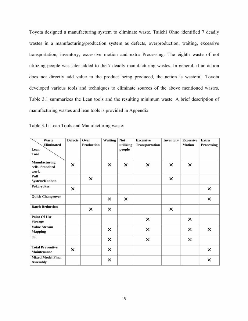
Toyota designed a manufacturing system to eliminate waste. Taiichi Ohno identified 7 deadly
wastes in a manufacturing/production system as defects, overproduction, waiting, excessive
transportation, inventory, excessive motion and extra Processing. The eighth waste of not
utilizing people was later added to the 7 deadly manufacturing wastes. In general, if an action
does not directly add value to the product being produced, the action is wasteful. Toyota
developed various tools and techniques to eliminate sources of the above mentioned wastes.
Table 3.1 summarizes the Lean tools and the resulting minimum waste. A brief description of
manufacturing wastes and lean tools is provided in Appendix
Table 3.1: Lean Tools and Manufacturing waste:
Waste Eliminated
Lean Tool
Defects Over Production
Waiting Not utilizing people
Excessive Transportation
Inventory Excessive Motion
Extra Processing
Manufacturing cells- Standard work
× × × × × ×
Pull System/Kanban
× ×
Poka-yokes × ×
Quick Changeover × × ×
Batch Reduction × × ×
Point Of Use Storage
× ×
Value Stream Mapping
× ×
× ×
5S × ×
×
Total Preventive Maintenance ×
× ×
Mixed Model Final Assembly
× ×
20
From the above table it can be seen that manufacturing cells are helpful in decreasing the source
of some of the above mentioned manufacturing wastes. In addition, manufacturing cells can lead
to higher operator utilization. Black (2003) states in a Lean enterprise the operators in the
manufacturing cells are multi-functional and multi-process, i.e., they can operate all machine
tools in the manufacturing cell and they can perform a variety of value added activities such as
problem solving, setup reduction, routine preventive maintenance, continuous improvement and
so on.
A manufacturing cell consists of a set of machine tools placed close to each other in series. Some
of the Machine tools in manufacturing cells are precise CNC machines. In some cases, a
manufacturing cell may even contain a small transfer line. The manufacturing cell is U-shaped so
that the first and the last process in the cell can be placed close to each other. Thus the operator
has a better control of the stock-on-hand in the cell. Black (2003) provides rules for
designing/implementing manufacturing cells – all the machine tools in the manufacturing cell
has machining/processing time less than the necessary cell cycle time and all the machine tools
in the manufacturing cell are simple yet precise single cycle automatic machine tools. Single
cycle automatics are an example of JIDOKA – separating machine’s task from operator’s task.
The manufacturing cell considered in this thesis has four CNC machine tools – Lathe,
Drilling/Boring machine, Milling machine and a center-less Grinding machine. It is a manned
manufacturing cell. The manufacturing cell machines a family of crankshafts and connecting
rods for lawnmower engines.

21
3.2 Transfer Lines:
A Transfer Line is a manufacturing system with a linear network of service stations or machines.
The work piece gets machined at every station of a transfer line and the transportation (the
transfer) between stations is automatic, which is accomplished through conveyer lines
connecting the stations. Because the work sequence of the part is fixed, automated material
handling systems are often found as link between stations. A raw work piece enters on one end
of the line, and manufacturing process is performed sequentially as the part progresses forward.
The line may include inspection stations for quality checks. Transfer lines have very high
production rates. Multiple parts are processed simultaneously, one part at each workstation. In
steady state the number of parts in the transfer line is equal to the number of stations in the
transfer line (Assuming no buffers are allocated in between stations). Each station performs
different tasks, so that all operations are required to complete one unit of work. Because all parts
flow through the same set of stations, the cycle times at each station must be about the same
duration. The capacity of the entire line will be determined by the longest cycle time. In other
words, the workstation with the longest cycle time sets the pace of that line. When a transfer line
has a fixture design specific to the geometry of work piece being machined, it is called a
palletized transfer line.
Transfer line is a very complex manufacturing system comprising of mechanical, electrical,
electronic, hydraulic / pneumatic and computer components. A transfer line has approximately
100,000 critical components which are essential for its operation. Due to its structure the
reliability of a transfer line cannot be greater than the reliability of its most unreliable station.
The complexity of the transfer line increases with the addition of stations. Also the reliability of
the transfer lines decreases with the addition of stations.

22
Groover (2001) mentions transfer lines are applicable only under the following conditions:
• High product demand requiring high product quantities
• Stable product design – Frequent design changes are difficult to cope with on an automated
production line
• Long product life, at least several years in most cases
• Multiple operations are performed on the product during its manufacture
In other words, transfer lines represent physical solutions to the above mentioned functional
requirements. Transfer lines have the advantage of having high production rates, reduced labor
requirements and floor space, etc.
Transfer lines represent highly automated manufacturing systems and are very common in
machining engine block castings, cylinder heads, crankshafts, etc. They are used in high volume
manufacturing/mass production environment. Transfer lines require a significant capital
investment, their capital costs range from $200,000 to $30,000,000. Since transfer lines are
capital intensive, they must be kept running to be economically justifiable.
The transfer line considered in this thesis is a 15-station automated transfer line which performs
a variety of drilling, boring, milling, honing operations for machining engine block castings,
cylinder heads and connecting rods. This transfer line has a production capacity of 1500 to 2000
units per 8 hour shift or about 0.25 minutes/part.

23
CHAPTER 4
Reliability in Manufacturing Systems Design
Manufacturing systems design (MSD) is a methodology of assembling machines, materials,
labor, material handling devices, computers, etc. to produce goods according to customer/design
requirements. Every manufacturing system is designed to deliver profit to the organization.
Mathematically, Profit ≈ Revenue – Cost. So to increase profit, sales must be increased and/or
the cost of making the goods has to be minimized. Manufacturing systems should be designed to
reduce costs. Manufacturing strategies that increases sales are quality of the product, reliability
of the product, product design, price reduction, etc. Some of the manufacturing strategies to
reduce manufacturing costs are WIP reduction, setup time reduction, labor reduction, defect
prevention (eliminates rework), etc.
The Ford motor company designed the first mass production system to reduce the manufacturing
cost through economy of scale. Toyota designed the first lean production system to eliminate
waste and reduce inventory thereby reducing the cost of manufacturing. Manufacturing systems
should be designed to decrease the operating cost by reduction and/or increasing sales through
better product quality & reliability.
Unreliable machines increase manufacturing costs. Unreliable machines can sometimes halt
entire production causing delays in the production and might also lead to scheduling problems.
In other words, unreliable machines increase manufacturing cost and thereby reduce profit.
Unreliable machines can also sometimes lead to unreliable products which create quality issues
which increases the warranty claims, recalls and reduces reputation of the organization which

24
affect the sales of the organization. Unreliable machines also increases the manufacturing lead
time which often leads to increases in buffer inventories.
The effect of unreliable machines on the manufacturing system’s performance is dependent on
its design. The severity of unreliable machines in cellular manufacturing and serial production
lines/transfer lines is greater than in a functional job shop. In a job shop, the machines are
grouped together by machine type (such as the lathe department, drilling department, etc.). In
case of a machine failure it can be easily rerouted to an available machine in that department. In
case of serial production lines/cellular layout, the unavailability of any one of the
machines/stations can lead to stoppage of the entire system. In cellular manufacturing, the
machines are grouped together and dedicated to machine a family of parts and failure of any one
machine tool will halt the entire production of the manufacturing cell.
Reliability should be a consideration in manufacturing systems design. But design for reliability
is an iterative process and should be improved on a continuous basis. To effectively improve
reliability, the life time of the critical components in the machines should be obtained. Once the
lifetime of the critical components is obtained, periodic replacement of those components can
prevent unplanned downtime of the machines. There are two approaches in lifetime testing –
empirical methods and reliability testing. In empirical methods, field failure data is collected and
fitted to statistical distributions. Reliability estimates are derived from parameters of the
statistical distribution. In reliability testing, the components are tested in an experimental setting
in attempt to generate failures in order to identify failure modes and eliminate them.
Reliability testing is not feasible for machine tools and production lines since the number of
components involved is very high. But reliability of machines could be improved by collecting

25
failure data and assessing reliability form the collected data. Once the failure data is obtained, it
can be fitted to a statistical distribution and the lifetime of components/systems can be estimated.
Collecting failure times and the reason for failures are necessary to improving the reliability of
manufacturing system.
Once reliability measures such as reliability function, mean time between failures and failure
rates are estimated, necessary maintenance and replacement techniques could be formulated to
improve manufacturing uptime.

26
CHAPTER 5
Reliability/Availability assessment of Manufacturing Cell
To assess and compare the reliability of manufacturing/machining cell versus a Transfer line,
failure data were collected from a manufacturing cell as well as a transfer line from a
manufacturing plant that produces small engines for lawn mowers. The manufacturing facility
machines the engine block castings and cylinder heads castings on its 15 station completely
palletized transfer line and the crankshafts that go into the engines are manufactured at the
manufacturing cell. The failure data correspond to the past three years of operations.
Manufacturing/Machining Cell:
The manufacturing/machining cell consists of four CNC machine tools, i.e., a lathe, milling
machine, drilling/boring machine and a Grinding machine.
27
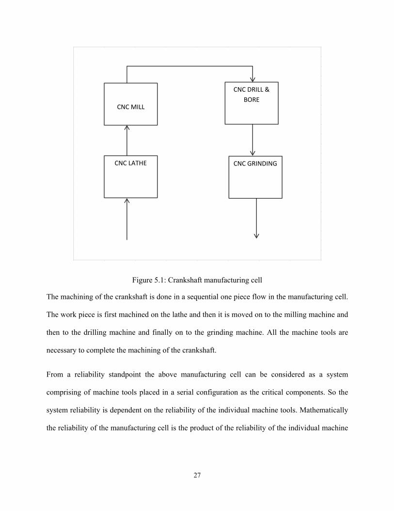
Figure 5.1: Crankshaft manufacturing cell
The machining of the crankshaft is done in a sequential one piece flow in the manufacturing cell.
The work piece is first machined on the lathe and then it is moved on to the milling machine and
then to the drilling machine and finally on to the grinding machine. All the machine tools are
necessary to complete the machining of the crankshaft.
From a reliability standpoint the above manufacturing cell can be considered as a system
comprising of machine tools placed in a serial configuration as the critical components. So the
system reliability is dependent on the reliability of the individual machine tools. Mathematically
the reliability of the manufacturing cell is the product of the reliability of the individual machine
CNC LATHE
CNC MILL
CNC DRILL & BORE
CNC GRINDING
28
tools. This implies that the reliability of the manufacturing cell can be no greater than that of the
most unreliable machine tool in the manufacturing cell.
Generally there are two approaches in fitting reliability distributions to failure data. The first
method is to fit a theoretical distribution. The second approach is to empirically derive the
reliability function and/or hazard function directly from the reliability data. The first approach is
better suited for the above problem as it presents the advantage of estimating the manufacturing
cell mean time between failures (MTBF) from the derived distributions.
The reliability of the manufacturing cell can be obtained from fitting the failure data into a
theoretical distribution. From the time between failures of individual machine tools, the failure
distribution of the individual machine tools can be obtained using goodness of fit tests. Then the
reliability measures for each of the individual machine tools can be obtained from their specific
failure distribution. After obtaining the reliability measures of the individual machine tools the
manufacturing cell reliability can be computed as the product of the reliability of the individual
machine tools.
Time between failure data from the manufacturing cell:
The time between failures of the individual machine tools and the reasons for failure for the
period of 3 years is given in Tables 5.1, 5.2, 5.3 and 5.4 below. The failure times are
field/operational failure times that were recorded as and when the failures occur and the failure
times are not censored. Also the failures of the machine tools are independent of each other.
The repair times were not usually recorded for the machine tool because whenever there is a
failure in the machine tool it is mostly not repairable such as electric motor burnt out, cutting tool
breakage, rheostat/fuse burn out, etc. So the part is usually replaced. If the time to repair times

29
are negligible when compared to the time between failures the reliability is the estimate of the
availability. Mathematically,
Availability = Uptime/ (Uptime +Downtime)
So when repair times are negligible Availability ≈ Reliability
Even though the repair time is negligible, it does represent some downtime. Unfortunately the
manufacturing facility does not record the repair time of their machine tools in their
manufacturing cell. This is because most of the time when failure occurs it results in replacement
not repair. But the operators and the maintenance engineer based on their experience denote that
the downtime/replacement time for their individual machine tools on an average is 1 hour.

30
Table 5.1: Time between failures of CNC lathe: (Source: Briggs and Stratton)
Time between failures, hours Reason For Failure 643 Spindle motor Failure 207 Electrical Relay failure 567 Cutting tool broken 252 Electric motor Damage 212 Fuse Burnt 216 Rheostat Failure 251 Coolant line clogged 190 Software Failure 354 Spindle motor Failure 109 Limit switch damaged 390 Pneumatic chuck failed to open 816 Stepper motor failure 500 Coolant pump failure 50 Transmission Failure 375 Turret Failure 553 Control Panel not Responding 303 Lubricant system failure 700 Fuse Burnt 351 Spindle Failure 187 Servo Motor Failure 157 Control Panel not Responding 284 Cutting tool broken 207 Pneumatic chuck failed to open 660 Internal Gear Failure 476 Electric motor Damage 652 Transmission Failure 658 Rheostat Failure 197 Coolant line clogged 107 Lubricant system failure 389 Stepper motor failure 86 Swarf Mechanism Failure
31
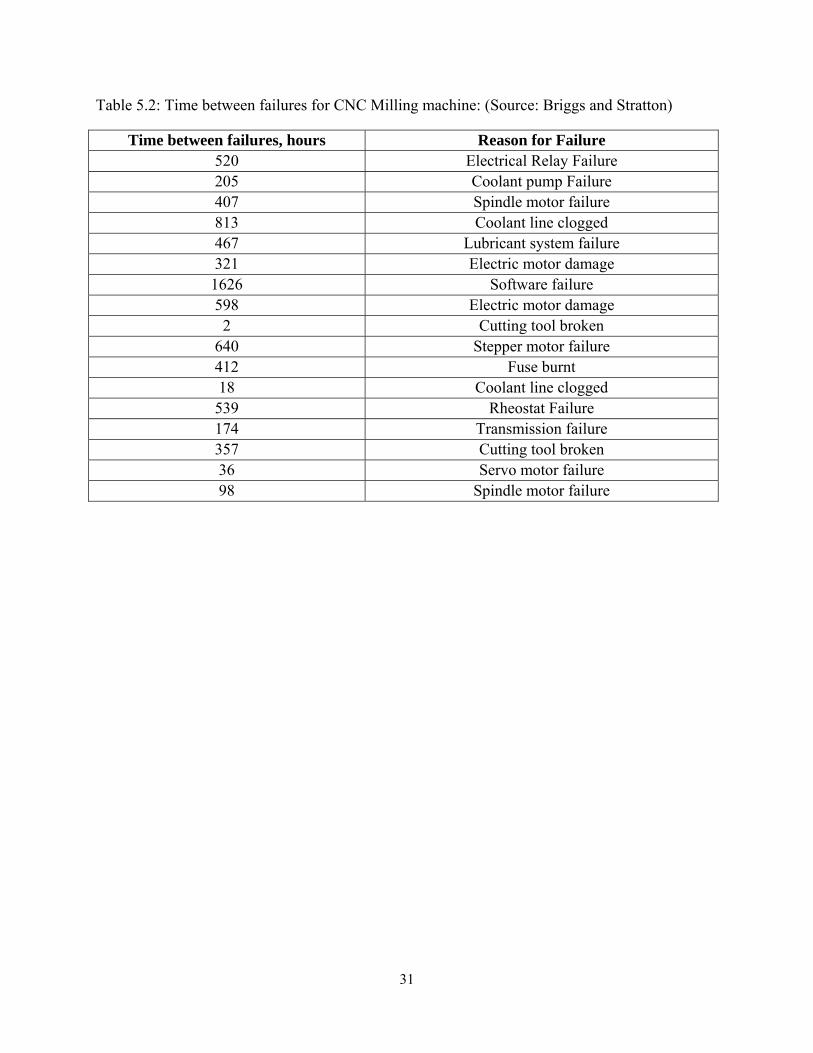
Table 5.2: Time between failures for CNC Milling machine: (Source: Briggs and Stratton)
Time between failures, hours Reason for Failure 520 Electrical Relay Failure 205 Coolant pump Failure 407 Spindle motor failure 813 Coolant line clogged 467 Lubricant system failure 321 Electric motor damage 1626 Software failure 598 Electric motor damage 2 Cutting tool broken
640 Stepper motor failure 412 Fuse burnt 18 Coolant line clogged 539 Rheostat Failure 174 Transmission failure 357 Cutting tool broken 36 Servo motor failure 98 Spindle motor failure

32
Table 5.3: Time between failures for CNC Drilling/Boring machine: (Source: Briggs and Stratton)
Time between failures, hours Reason for Failure 827 Cutting tool broken 464 Spindle motor Failure 568 Electric motor Damage 503 Automatic Tool change failure 558 Electrical Relay failure 104 Coolant pump failure 254 Electrical Relay failure 187 Control Panel not Responding 884 Stepper motor failure 456 Fuse Burnt 64 Pneumatic chuck failed to open 113 Transmission Failure 302 Cutting tool broken 739 Spindle motor Failure 313 Electric motor Damage 342 Lubricant system failure 229 Automatic Tool change failure 733 Electric motor Damage 89 Stepper motor failure 210 Electrical Relay failure 293 Cutting tool broken 156 Automatic Tool change failure 581 Coolant line clogged 779 Electrical Relay failure 305 Stepper motor failure 23 Electric motor Damage 412 Rheostat Failure 376 Spindle motor Failure 472 Cutting tool broken 493 Fuse Burnt 676 Control Panel not Responding 153 Pneumatic chuck failed to open 436 Transmission Failure 715 Turret Failure

33
Table 5.4: Time between failures of CNC Grinding machine (Source: Briggs and Stratton)
Time between failures, hours Reason for Failure 1065 Grinding wheel wear 868 Software failure 785 Electrical relay failure 742 Grinding wheel wear 572 Fuse burnt 72 Electrical motor damage 448 Rheostat failure 831 Spindle motor failure 223 Transmission failure 485 Grinding wheel wear 454 Stepper motor damage 144 Electrical relay failure 93 Servo motor failure 756 Grinding wheel wear 689 Pneumatic chuck fail to open 816 Spindle motor failure
The above failure data for the individual machine tool can be fit into a relevant theoretical
distribution using goodness of fit tests. But before using the goodness of fit tests it should be
noted that the above failures are caused by different failure modes. Usually in Reliability
engineering when estimating product reliability it is not a recommended practice to mix the
failure times from various failure modes. But the following analysis is for estimating process
reliability (which is the availability) rather than product reliability. In other words the focus here
is on how long/how often the machine is unavailable so that it affects the production rather than
by what mode it failed. Also the lack of availability of sufficient data for each failure modes
makes it impractical to estimate the reliability measures for each failure modes. The above task
could be better accomplished by reliability testing on machine tools rather than collecting field
failure data.
34
5.1 Identifying appropriate TBF distribution for individual machine tools in crankshaft
manufacturing cell:
5.1.1 CNC Lathe:
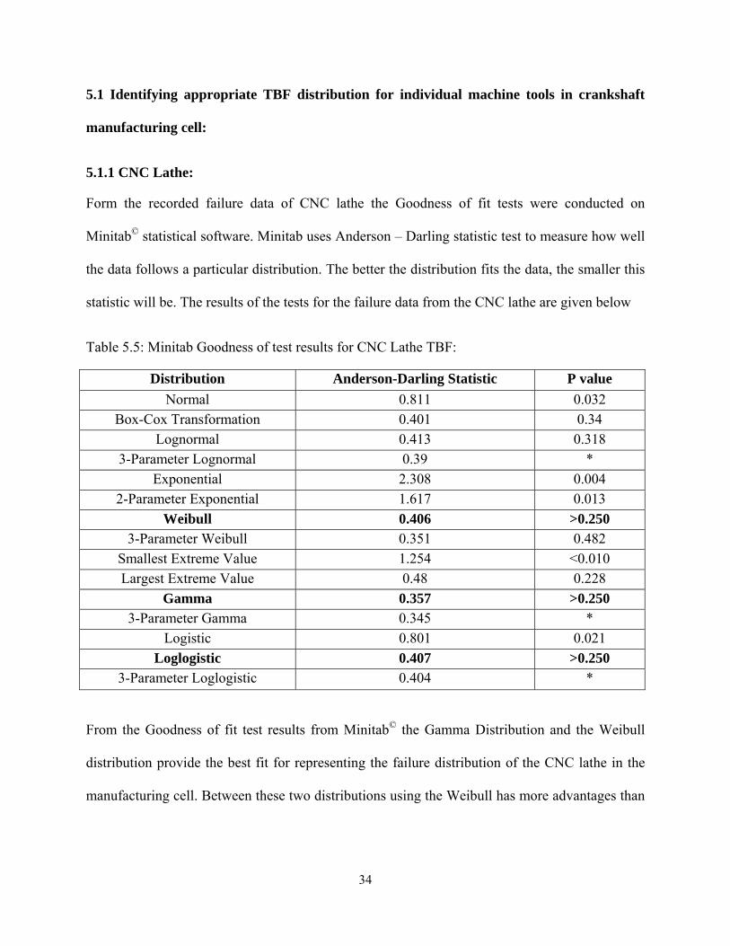
Form the recorded failure data of CNC lathe the Goodness of fit tests were conducted on
Minitab© statistical software. Minitab uses Anderson – Darling statistic test to measure how well
the data follows a particular distribution. The better the distribution fits the data, the smaller this
statistic will be. The results of the tests for the failure data from the CNC lathe are given below
Table 5.5: Minitab Goodness of test results for CNC Lathe TBF:
Distribution Anderson-Darling Statistic P value Normal 0.811 0.032
Box-Cox Transformation 0.401 0.34 Lognormal 0.413 0.318
3-Parameter Lognormal 0.39 * Exponential 2.308 0.004
2-Parameter Exponential 1.617 0.013 Weibull 0.406 >0.250
3-Parameter Weibull 0.351 0.482 Smallest Extreme Value 1.254 <0.010 Largest Extreme Value 0.48 0.228
Gamma 0.357 >0.250 3-Parameter Gamma 0.345 *
Logistic 0.801 0.021 Loglogistic 0.407 >0.250
3-Parameter Loglogistic 0.404 *
From the Goodness of fit test results from Minitab© the Gamma Distribution and the Weibull
distribution provide the best fit for representing the failure distribution of the CNC lathe in the
manufacturing cell. Between these two distributions using the Weibull has more advantages than

35
the gamma distribution because the Weibull shape parameter β gives a good description of type
of failure (See table below).
Weibull Shape parameter (β) Representation of β<1 Infant mortality (Decreasing failure rate) β=1 Constant failure rate β>1 Increasing failure rate, Wear out failures
Before estimating the Weibull parameters a Weibull goodness of fit test must be conducted to
make sure that the failure times is Weibull distributed, also Minitab© only gives approximate P
values for the Weibull fit (>0.250) and the Weibull goodness of fit is required to obtain the exact
P value to justify the use of the Weibull distribution to represent the failure times of the CNC
lathes.
Mann’s Test for the Weibull Distribution:
A goodness of fit test for the Weibull distribution is a test developed by Mann, Schafer and
Singpurwalla [1974]. The hypotheses are
H0: The failure times are Weibull
H1: The failure times are not Weibull
The test statistic is
1
1
1 11
1
2 11
[(ln ln )/ ]
[(ln ln ) / ]
r
i i ii k
k
i i ii
k t t MM
k t t M
−
+= +
+=
−=
−
∑
∑
Where 1 2rk ⎢ ⎥= ⎢ ⎥⎣ ⎦
21
2rk −⎢ ⎥= ⎢ ⎥⎣ ⎦

36
Mi = Zi+1 – Zi
0.5ln[ ln(1 )]0.25i
iZn
−= − −
+
r = n = number of failures and x⎢ ⎥⎣ ⎦ is the integer portion of x . If2 1,2 ,2k kM Fα> ,then the null
hypothesis is rejected. Values of Fα can be obtained from tables of F-distribution for a specified
critical value α where the numerator degrees of freedom is 2k2 and denominator degrees of
freedom is 2k1.
For the failure times of the CNC lathe the value of n = r = 31 and k1 = k2 = 15.
The M statistic calculated from the above formula is M = 1.264983
The critical value is F0.05, 30, 30 is F0.05, 30, 30 = 1.840872, which shows that M < F0.05, 30, 30. So the
decision is to fail to reject the null hypothesis and conclude that the failure times are Weibull
distributed with 95% confidence. The P value from the above test is 0.60 which is sufficiently
large to support the decision of failing to reject H0 at the 5% level.
The Weibull Distribution:
The 2-parameter Weibull distribution is a continuous distribution that may be used to represent
increasing/decreasing/constant failure rates. It is characterized by parameters β and θ, where β is
the shape parameter for Weibull distribution and θ is the characteristic life of the Weibull
distribution.
Estimating the Weibull parameters β and θ using Maximum likelihood estimation (MLE):
The probability density function (pdf), f (t) of the 2-parameter Weibull distribution is given by
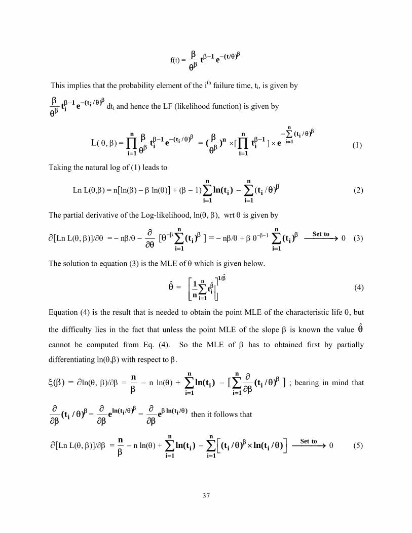
37
f(t) = 1 (t/ )t eββ− − θ
ββ
θ
This implies that the probability element of the ith failure time, ti, is given by
i(t / )1it e
β− θβ−β
βθ
dti and hence the LF (likelihood function) is given by
L( θ, β) = in
(t / )1i
i 1t e
β− θβ−β
=
βθ
∏ = n( )ββθ
×[n
1i
i 1tβ−
=∏ ] ×
ni
i 1(t / )
eβ
=− θ∑
(1)
Taking the natural log of (1) leads to
Ln L(θ,β) = n[ln(β) − β ln(θ)] + (β − 1)n
ii 1
ln(t )=∑ − ( / )
n
ii 1
t β
=θ∑ (2)
The partial derivative of the Log-likelihood, ln(θ, β), wrt θ is given by
∂[Ln L(θ, β)]/∂θ = − nβ/θ − ∂∂θ
[θ−βn
ii 1
(t )β
=∑ ] = − nβ/θ + β θ−β−1
n
ii 1
(t )β
=∑ Set to⎯⎯⎯→ 0 (3)
The solution to equation (3) is the MLE of θ which is given below.
θ̂ = ˆ1/n ˆ
ii 1
1 tn
ββ
=
⎡ ⎤⎢ ⎥⎢ ⎥⎣ ⎦
∑ (4)
Equation (4) is the result that is needed to obtain the point MLE of the characteristic life θ, but
the difficulty lies in the fact that unless the point MLE of the slope β is known the value θ̂
cannot be computed from Eq. (4). So the MLE of β has to obtained first by partially
differentiating ln(θ,β) with respect to β.
ξ(β) = ∂ln(θ, β)/∂β = nβ
− n ln(θ) + n
ii 1
ln(t )=∑ − [
n
ii 1
(t / )β
=
∂θ
∂β∑ ] ; bearing in mind that
i(t / )β∂θ
∂β= iln(t / )e
βθ∂∂β
= iln(t / )eβ θ∂∂β
then it follows that
∂[Ln L(θ, β)]/∂β = nβ
− n ln(θ) + n
ii 1
ln(t )=∑ −
n
i ii 1
(t / ) ln(t / )β
=
⎡ ⎤θ × θ⎣ ⎦∑ Set to⎯⎯⎯→ 0 (5)

38
Equations (4) & (5) will have to be solved simultaneously in order to obtain the Maximum
likelihood estimates of θ and β. Unfortunately, no closed-form exists for θ̂ and β̂ . Therefore,
the solutions have to be obtained through trial and error that will make both partial derivatives
∂ln(θ, β)/∂θ in (3) and ∂ln(θ, β)/∂β in (5) almost equal to zero. The above task can be
accomplished through the Newton-Raphson algorithm.
Estimating the Weibull parameters for CNC Lathe:
Using the above mentioned maximum likelihood estimation procedure the Weibull parameter
estimates for CNC lathe can be estimated using the time between failure data of the CNC lathe
provided in Table 1. The parameter estimates is obtained using the following steps
(1) Arrange the time between failures data ti’s from smallest to largest, i.e. order the statistic,
where the first order statistic represents the smallest time between failure data, the second
order statistic the next smallest failure time and so on.
(2) Select an arbitrary value for β. A logical selection would be β greater than 1 because the
CNC lathe is experiencing wear out failures as suggested from the data in Table 1.
Elsayed (1996) also provides a good starting approximation of β which is given by β̂ =
1.05/CV, where CV is the sample coefficient of variation from the failure data.
(3) Obtain the value of θ̂ using equation (4) and the arbitrary value of β. substitute the
values of θ and β in equation (5)
(4) Continuously solve for different values of β and θ that makes the equation (5) almost
zero to obtain the exact estimates of β and θ for the given Weibull data. This can be
solved Newton-Raphson algorithm using an appropriate software program.
39
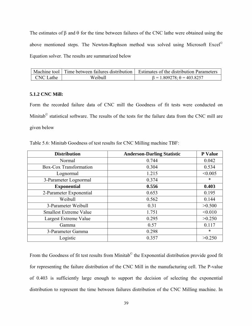
The estimates of β and θ for the time between failures of the CNC lathe were obtained using the
above mentioned steps. The Newton-Raphson method was solved using Microsoft Excel©
Equation solver. The results are summarized below
Machine tool Time between failures distribution Estimates of the distribution Parameters CNC Lathe Weibull β = 1.809278; θ = 403.8257
5.1.2 CNC Mill:
Form the recorded failure data of CNC mill the Goodness of fit tests were conducted on
Minitab© statistical software. The results of the tests for the failure data from the CNC mill are
given below
Table 5.6: Minitab Goodness of test results for CNC Milling machine TBF:
Distribution Anderson-Darling Statistic P Value Normal 0.744 0.042
Box-Cox Transformation 0.304 0.534 Lognormal 1.215 <0.005
3-Parameter Lognormal 0.374 * Exponential 0.556 0.403
2-Parameter Exponential 0.653 0.195 Weibull 0.562 0.144
3-Parameter Weibull 0.31 >0.500 Smallest Extreme Value 1.751 <0.010 Largest Extreme Value 0.295 >0.250
Gamma 0.57 0.117 3-Parameter Gamma 0.298 *
Logistic 0.357 >0.250
From the Goodness of fit test results from Minitab© the Exponential distribution provide good fit
for representing the failure distribution of the CNC Mill in the manufacturing cell. The P-value
of 0.403 is sufficiently large enough to support the decision of selecting the exponential
distribution to represent the time between failures distribution of the CNC Milling machine. In

40
addition the coefficient of variation (CV) of the time between failures data of the CNC milling
machine is 0.9146 which is close to 1. So keeping in mind that exponential distribution has
theoretical coefficient of variation of 1, the CV value of 0.9146 is sufficiently close to 1 to
support the fact that the time between failure data for CNC milling machine is approximately
exponentially distributed.
The Exponential Distribution:
The exponential distribution is a continuous distribution that is used to represent the constant
failure rates. It is characterized by the parameter λ which represents the failure rate of the
component (or system). The failure rate λ of the exponential distribution is constant with respect
to time; this property of the exponential distribution is called the “memorylessness” property, i.e.
is the time to failure of the component is independent of how long it has been operating. The
exponential is the only continuous distribution in the universe with the memorylessness property.
The exponential distribution is characterized only by its failure rate parameter λ, so if the
parameter λ can be estimated, all the other reliability measures can be obtained from λ.
Estimating the Exponential parameter (λ) using Maximum likelihood estimation (MLE) :
The probability density function of an exponential random variable (pdf), f (t) is given by
( ) tf t e λλ −= (6)
This implies that the probability element of the ith failure time, ti, is given by ite λλ − dti and
hence the likelihood function is given by

41
1
( ) i
nt
i
L e λλ λ −
=
= ∏
1( )
n
ii
tnL e
λ
λ λ =
− ∑=
Taking natural logarithm on both sides
1ln[ ( )] ln[ ]
n
ii
tnL e
λ
λ λ =
− ∑=
1ln[ ( )] ln( )
n
ii
L n tλ λ λ=
= − ∑
Taking derivative with respect to λ
1[ln( ( ))]
n
ii
nL tλλ λ =
∂= −
∂ ∑ Set to⎯⎯⎯→ 0
1ˆn
ii
n tλ =
= ∑
1
ˆn
ii
n
tλ
=
=
∑ (7)
Equation (7) is the maximum likelihood estimate for the exponential distribution with failure rate
λ. So the failure rate λ for the CNC milling machine can be found out using the time between
failures data’s from Table 2. From the time between failures data from table 2 and using equation
(7) the failure rate λ for the CNC milling machine is estimated as
Machine tool Time between failures distribution Estimates of the distribution Parameters CNC Mill Exponential λ=0.030323 per hour

42
5.1.3 CNC Drilling and Boring machine:
Form the recorded failure data of CNC drilling and boring machine the Goodness of fit tests
were conducted on Minitab© statistical software. The results of the tests for the failure data from
the CNC drilling and boring machine are given below
Table 5.7: Minitab Goodness of test results for CNC Drilling & Boring machine TBF:
Distribution Anderson-Darling Statistic P Value
Normal 0.345 0.464
Box-Cox Transformation 0.234 0.778
Lognormal 0.883 0.021
3-Parameter Lognormal 0.277 *
Exponential 2.082 0.007
2-Parameter Exponential 2.095 <0.010
Weibull 0.265 >0.250
3-Parameter Weibull 0.243 >0.500
Smallest Extreme Value 0.773 0.041
Largest Extreme Value 0.297 >0.250
Gamma 0.393 >0.250
3-Parameter Gamma 0.28 *
Logistic 0.379 >0.250
Loglogistic 0.634 0.061
3-Parameter Loglogistic 0.319 *
From the above results the Weibull distribution is the most appropriate for fitting the failure
times. The P-value of more than 0.250 is sufficient enough to support the selection of the
Weibull distribution to represent the failure time distribution for the CNC drilling/boring

43
machine. The exact P-value using the Mann’s goodness of fit test for Weibull distribution
developed before is 0.905. Using the same procedure as developed for CNC lathe for estimating
the Weibull parameters the Weibull parameter estimates for the CNC drilling/boring machine is
given below
Machine tool Time between failures distribution Estimates of the distribution ParametersCNC Drill/Bore Weibull β = 1.718139; θ = 453.7725
5.1.4 CNC Grinding machine:
Form the recorded failure data of CNC grinding machine the Goodness of fit tests were
conducted on Minitab© statistical software. The results of the tests for the failure data from the
CNC grinding machine are given below
Table 5.8: Minitab Goodness of test results for CNC Grinding machine TBF:
Distribution Anderson-Darling Statistic P Value
Normal 0.459 0.228
Box-Cox Transformation 0.459 0.228
Lognormal 1.213 <0.005
3-Parameter Lognormal 0.5 *
Exponential 1.525 0.026
2-Parameter Exponential 1.501 0.011
Weibull 0.846 0.024
3-Parameter Weibull 0.406 0.259
Smallest Extreme Value 0.324 >0.250
Largest Extreme Value 0.718 0.051
Gamma 0.954 0.02
3-Parameter Gamma 0.765 *
Logistic 0.476 0.188

44
Loglogistic 1.077 <0.005
3-Parameter Loglogistic 0.479 *
From the above results the smallest extreme value distribution is the only distribution that is
appropriate for fitting the failure times for the CNC grinding machine.
The smallest extreme value distribution:
The smallest extreme value distribution is closely related to the Weibull distribution in that if the
time between failures (TBF) has a Weibull distribution, then log(TBF) has an extreme value
distribution. Lawless (2003) states that an extreme value distribution is an asymptotic
distribution resulting from finding the minimum or maximum of a large number of observations
from an underlying unbounded population.
Estimating the Smallest extreme value parameters α and μ using Maximum likelihood
estimation (MLE):
The probability density function (pdf), f(t) for the smallest extreme value distribution is given by
( )( )1( ) ( )tiit
ef t e eμ
αμ
α
α
−−−= , (8)
where α is the scale parameter and μ is the location parameter of the smallest extreme value
distribution. The likelihood function L(α, μ) is given by
( )( )( )( )
1
1( , ) ( )ti
itne
i
L e eμ
αμ
αα μα
−−−
=
= ∏ (9)
Taking natural logarithm on both sides

45
( )
1 1
( )ln[ ( , )] lnitn n
i
i i
tL n eμ
αμμ α αα
−
= =
−= − + −∑ ∑
Maximum likelihood estimates can be found by taking the partial derivatives of the log
likelihood function with respect to α and then μ and equating them to zero, i.e. by setting
ln ( , ) ln ( , ) 0L Lα μ α μα μ
∂ ∂= =
∂ ∂
and solving for α and μ. Following Lawless (2003), ln ( , ) 0L α μμ
∂=
∂ can be solved for μ
1
1ln[ ]itn
ie
rαμ α
=
= ∑ (10)
, substituting this into ln ( , )L α μα
∂∂
=0 results in:
1
1
1
1 0
i
i
tn
ini
i tni
i
t et
ne
α
α
α =
=
=
− − + =∑
∑∑
(11)
Equations (10) and (11) can be solved numerically for α and μ by the Newton-Raphson
procedure mentioned previously with the help of Microsoft Excel© solver. The results are
summarized below
Machine tool Time between failures distribution Estimates of the distribution Parameters
CNC Grinder Smallest extreme value α = 251.628; μ = 707.3796

46
Summary of distribution parameter(s) estimates for the machine tools in the
manufacturing cell:
Thus far the appropriate distributions for the time between failures of the machine tools in the
manufacturing cell has been determined by Goodness of fit tests for specific distributions and the
parameter estimate(s) for the individual distributions have been determined by maximum
likelihood estimation. Once the individual distribution and the distribution parameters for the
time between failures of the machine tools are estimated all the reliability measures such as the
reliability function, hazard rate function and the Mean time between failures (MTBF’s) for the
individual machine tools and hence the manufacturing cell reliability measures can be estimated.
The summary of the results of the estimations thus far are given below
Table 5.9: Distribution parameter(s) estimates for the machine tools in the manufacturing cell:
Machine tool Time between failures distribution Estimates of the distribution
Parameters
CNC Lathe Weibull β = 1.809278; θ = 403.8257
CNC Mill Exponential λ=0.00279
CNC Drill/Bore Weibull β = 1.718139; θ = 453.7725
CNC Grind Smallest extreme value α = 251.628; μ = 707.3796

47
5.2 Reliability measures for the machine tools in the manufacturing cell:
As mentioned previously, reliability is the probability that a component (or) equipment will
perform a required function for a given period of time when used under stated operating
conditions. The most commonly used reliability measures in manufacturing are point reliability
function (reliability for a specified time period) and mean time between failures. Before
assessing the point reliability of the individual machine tools, the term specified time period has
to be decided. The manufacturing facility from which the failure data was collected has a
scheduled monthly preventive maintenance, so a good time period would be one month
(approximately 160 hours). For now it is assumed that the preventive maintenance increases the
time between failures of the machines. In other words, for the case mentioned above, a machine
tool is considered available if it does not breakdown or fail for 160 hours of its operation or if the
time to failure exceeds 160 hours of operation. Mathematically it can be expressed as
( ) Pr( )R t T t= >
, where T is the time between failure (TBF), with Pr (Probability) density function f(t). So
( ) Pr( ) ( )t
R t T t f t dt∞
= > = ∫
The pdf (Pr density function), f(t) is also referred to as failure (or mortality) density function.
The Reliability function R(t) can also be expressed in terms of the cumulative density function
F(t), which is the cumulative failure probability by time t.
( ) Pr( ) ( ) 1 Pr( ) 1 ( )
t
R t T t f t dt T t F t∞
= > = = − ≤ = −∫ (12)
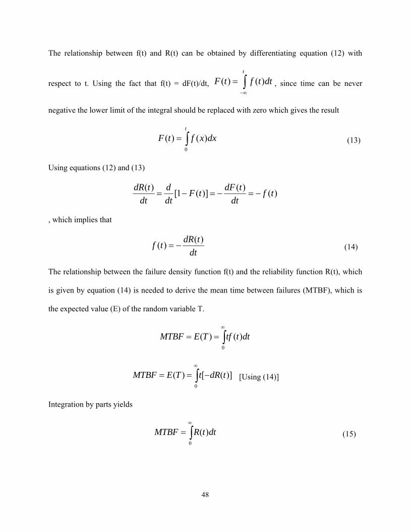
48
The relationship between f(t) and R(t) can be obtained by differentiating equation (12) with
respect to t. Using the fact that f(t) = dF(t)/dt, ( ) ( )t
F t f t dt−∞
= ∫ , since time can be never
negative the lower limit of the integral should be replaced with zero which gives the result
0
( ) ( )t
F t f x dx= ∫ (13)
Using equations (12) and (13)
( ) ( )[1 ( )] ( )dR t d dF tF t f tdt dt dt
= − = − = −
, which implies that
( )( ) dR tf tdt
= − (14)
The relationship between the failure density function f(t) and the reliability function R(t), which
is given by equation (14) is needed to derive the mean time between failures (MTBF), which is
the expected value (E) of the random variable T.
0
( ) ( )MTBF E T tf t dt∞
= = ∫
0
( ) [ ( )]MTBF E T t dR t∞
= = −∫ [Using (14)]
Integration by parts yields
0
( )MTBF R t dt∞
= ∫ (15)

49
Using the above derived reliability measures the reliability of the individual machine tools over a
specified time period and their respective mean time between failures can be determined. As
mentioned previously the time period for all the forthcoming calculations would be 160 hours (1
month period).
5.2.1 CNC Lathe:
The time between failures for CNC lathe follows Weibull distribution (see Table 2). The
probability density function f(t) of the 2 parameter Weibull distribution is given by
1 ( / )( ) tf t t eββ θ
β
βθ
− −=
Using (12)
1 ( / )( ) tLATHE
t
R t t e dtββ θ
β
βθ
∞− −= ∫
Solving the above expression through integration by parts yields
( / )( ) t
LATHER t eβθ−= (16)
Substituting the values of θ = 403.8257 and β = 1.809278 obtained earlier for CNC lathe time
between failures through maximum likelihood estimation into equation (16) yields
(160 ) 0.829196LATHER hours =
The mean time between failures for the CNC lathe can be estimated from equation (15)
( / )
0
tLATHEMTBF e dt
βθ∞
−= ∫
Making the transformation x = (t/θ)β in the above integral results in
50
1/ 1
0
1 ( )xLATHEMTBF e x dxβ βθ
β
∞− −= ∫
(1/ ) 1
0
1 xx e dxβθβ
∞− −= ∫
By definition a gamma random variable ( )nΓ is defined by
1
0
( ) n xn x e dx∞
− −Γ = ∫
Using the above fact, the MTBF can be rewritten as
1 (1/ )LATHEMTBF θ ββ
= Γ
Using the property of the gamma function, ( ) ( 1)n n nΓ = Γ + the MTBF equation becomes
(1 1/ )LATHEMTBF θ β= ×Γ + (17)
Substituting the values of θ = 403.8257 and β = 1.809278 obtained earlier for CNC lathe time
between failures through maximum likelihood estimation into equation (17) yields
359.029LATHEMTBF hours=
5.2.2 CNC Mill:
The time between failures for CNC milling machine follows Exponential distribution (see Table
3.5). The probability density function f(t) of the Exponential distribution is given by

51
( ) tf t e λλ −=
Using (12)
( ) xMILL
t
R t e dxλλ∞
−= ∫
Solving the above integral results in
( ) t
MILLR t e λ−= (18)
Substituting the values of λ = 0.00279 obtained earlier for CNC mill time between failures
through maximum likelihood estimation into equation (18) yields
(160 ) 0.686875MILLR hours =
Using equation (15)
0
tMILLMTBF e dtλ
∞−= ∫
1MILLMTBF
λ= (19)
Substituting the value of λ = 0.00279 in the above equation gives
425.4706MILLMTBF hours=

52
5.2.3 CNC Drill/Bore:
The time between failures for CNC Drill follows Weibull distribution (see Table 3.5).Using the
exact same procedure as developed for CNC lathe
(160 ) 0.846378DRILLR hours =
404.5914DRILLMTBF hours=
5.2.4 CNC Grind:
The time between failures for the CNC grinding machine follows the smallest extreme value
distribution. The probability density function (pdf), f(t) for the smallest extreme value
distribution is given by
( )( )1( ) ( )tt
ef t e eμ
αμ
α
α
−−−=
The reliability function of the smallest extreme value can be derived using its relationship with
the Weibull distribution. By definition if a random variable X has a Weibull time between failure
distribution then its natural logarithm, T=ln(X) has a minimum extreme value distribution. To
arrive at the reliability function of the smallest extreme value, let F(x) represent the cdf of the
Weibull distribution and let G(t) represent the cdf of t=ln(x), and R(t) is the reliability function of
T. Then by definition
( ) Pr( ) Pr(ln( ) ) Pr( ) ( )t tG t T t X t X e F e= ≤ = ≤ = ≤ =
As mentioned previously if a random variable X has a Weibull time between failure distribution
then its natural logarithm, T=ln(X) has a minimum extreme value distribution. In other words the
53
time between failures has a smallest extreme value distribution if and only if X=et has the
Weibull distribution. So the above expression can be written as
( ) ( ) ( )t tT XF e R t R e= =
Using the reliability function of the Weibull distribution derived earlier the above expression can
be rewritten as
( / )( ) exp[ ]t tXR e e
βθ−=
Simplifying the above expression yields the reliability function for the smallest extreme value
distribution
( )/exp[ ]t
GRINDR e μ α−= − (20)
Substituting the values of α=251.628 and μ=707.3096 obtained earlier for CNC grinding
machine time between failures through maximum likelihood estimation into equation (20) yields
(160 ) 0.892643GRINDR hours =
The mean time between failures for the smallest extreme value distribution is difficult to obtain,
Ebeling (1997) provides the results of the MTBF expression for smallest extreme value
distribution. Following Ebeling (1997),
GRINDMTBF μ αγ= − (21)
, where γ=0.5772157 is the irrational Euler’s constant defined by 1
lim (1/ ) log ( )n
en ii nγ
→∞=
⎡ ⎤= −⎢ ⎥
⎣ ⎦∑
Substituting the values of α=251.628 and μ=707.3096 in the above equation results in
562.136GRINDMTBF hours=

54
The manufacturing cell reliability can now be estimated since the necessary reliability measures
for all the individual machine tools in the manufacturing cell have been determined.
5.3 Manufacturing cell reliability estimation:
As seen in figure 1 the crankshaft manufacturing/machining cell is comprised of four CNC
machine tools: Lathe, milling machine, drilling/boring machine and a grinding machine. To
produce a finished steel crankshaft, the crankshaft casting needs to be machined on all four
machine tools in the manufacturing cell. The above case is very much similar to a system of four
serially connected machines in which for the system to be reliable all four machines must be
reliable. In other words, the system fails if any one of the four machines fails. So for the
crankshaft manufacturing/machining cell all four machine tools must function reliably during the
mission interval for the manufacturing cell, to produce the products. The reliability of the
individual machine tools is a decreasing function of time. Furthermore the reliability of the
manufacturing cell with serially placed machine tools can be no greater than that of the
individual machine tools. More specifically the reliability of the manufacturing cell can be no
greater than that of the least reliable machine tool in the manufacturing cell. For a serial system
the system reliability is the product of the individual components reliability.
MANUFACTURINGCELL LATHE DRILL MILL GRINDR R R R R= × × × (22)
So the manufacturing cell reliability for 160 hours of operation/mission time would be the
product of the reliability of the individual machine tools for 160 hours of operation. Substituting
the values individual reliability of machine tools at 160 hours yields the manufacturing cell
reliability.
(160 ) 0.430112MANUFACTURINGCELLR hours =

55
5.4 Manufacturing Cell Availability Estimation:
The instantaneous availability of a system with n serially connected components is given by
1 2
1(1/ ) (1/ ) ...... (1/ )SYS
n
MTBFMTBF MTBF MTBF
=+ + +
So for a serially connected manufacturing cell with a lathe, drill, mill and grinder, the MTBFSYS
reduces to
1(1/ ) (1/ ) (1/ ) (1/ )MANUFACTURINGCELL
LATHE MILL DRILL GRIND
MTBFMTBF MTBF MTBF MTBF
=+ + +
Substituting the MTBF of the individual machine tools in the above equation yields
106.539529MANUFACTURINGCELLMTBF hours= (23)
To compute the availability of the manufacturing cell, the mean time to repair for each of the
individual machine tools is needed. Unfortunately, the manufacturing facility from which the
data was collected does not record the repair time of the individual machine tools after failure
occurs. This is because, most of the time, when failure occurs it results in replacement not repair.
But the operators and the maintenance engineer based on their experience denote that the
downtime/replacement time for their individual machine tools on an average is no more than 1
hour. So the repair time for each of the machine tool in the manufacturing cell will be assumed to
be 1 hour for this analysis.
1(1/ ) (1/ ) (1/ ) (1/ )MANUFACTURINGCELL
LATHE MILL DRILL GRIND
MTTRMTTR MTTR MTTR MTTR
=+ + +
When the time to repair for each of the machine tool is assumed to be the same the above
equation reduces to

56
1
1MANUFACTURINGCELL n
ii
MTTRMTTR
=
=
∑
Substituting the MTTR=1 hour in the above equation yields
0.25MANUFACTURINGCELLMTTR hours= (24)
By definition the instantaneous availability is defined as
( )
UPTIMEAvailabilityUPTIME DOWNTIME
=+
(25)
Mathematically that is equivalent to
( )
MTBFAvailabilityMTBF MTTR
=+
(26)
Substituting (32) and (33) in (35) gives the availability of transfer line
0.99765895MANUFACTURINGCELLAvailability =
5.5 Reliability Estimation – Sensitivity Analysis:
Until now the Reliability of the manufacturing cell for 160 hours (1 month) of the plants
operation has been considered. The manufacturing facility from which the data was collected has
a daily preventive maintenance (Routine cleaning), a weekly preventive maintenance
(Lubrication) and a monthly preventive maintenance (Replacement, Overhauling, etc.). So it is
appropriate to obtain the reliability estimate for the above mentioned time periods to assess the
probability of machine tools/manufacturing cell not failing in-between the scheduled
maintenance operations.
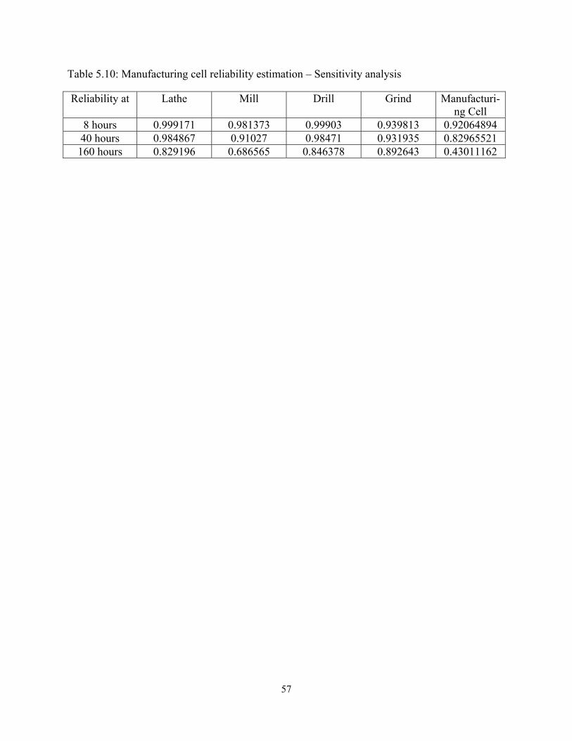
57
Table 5.10: Manufacturing cell reliability estimation – Sensitivity analysis
Reliability at Lathe Mill Drill Grind Manufacturi-ng Cell
8 hours 0.999171 0.981373 0.99903 0.939813 0.92064894 40 hours 0.984867 0.91027 0.98471 0.931935 0.82965521 160 hours 0.829196 0.686565 0.846378 0.892643 0.43011162

58
CHAPTER 6
Reliability/Availability assessment of Transfer Line
The transfer line that is considered in the study is a 15-station completely automated transfer line
which machines engine block castings for lawnmowers. The transfer line performs various
drilling, milling, boring and honing operations on the engine block castings. A transfer line is a
linear network of machines or service stations. Material flows from outside the system to
station1, then to station2, and so forth until it reaches station 15 after which it exits for assembly.
Figure 6.1: A 15 station palletized Transfer line
A transfer line is a complex manufacturing system comprising of mechanical, electrical,
hydraulic and numerical control components. The engine block machined on the transfer line
goes through each and every station in the transfer line in order to be machined completely. So
for transfer line to operate reliably, all the stations in the transfer line must be available. Failure
in any one of the stations will cause the line to shut down completely. From a reliability
Station 1
Station 15
59
standpoint, the transfer line shown in figure 6.1 can be considered as a system comprised of
machining stations placed in a serial configuration. As the number of stations along the transfer
line increases, the probability of all stations being operational decreases. The system reliability is
dependent on the reliability of the individual stations reliability. Mathematically the reliability of
the transfer line is the product of the reliability of the individual stations. This implies that the
reliability of the manufacturing cell can be no greater than that of the most unreliable station in
the transfer line. Unfortunately, due to the lack of sufficient failure data from each of the stations
and due to the fact that some failure data are not specific to a particular station but to the entire
system, the transfer line is considered as a single system for the forthcoming calculations. This
assumption is realistic because the transfer line is unavailable regardless of which station fails
first.
Time between failure data from the transfer line:
The time between failures (TBF) of the transfer line, the time to repair (TTR) and the reasons for
failure for the period of 3 years is given in Tables 5 below. The failure times are field/operational
failures that were recorded when failures occurred and the failure times were not censored. Also
the failures of the stations are independent of each other.

60
Table 6.1: Time between failures and time to repair for 3 years for a 15 station palletized
Transfer line: (Source: Briggs and Stratton)
Time between Failures, hours
Time to repair, hours
Reason For failure
80 1.5 Proximity Switch Damaged 3 1 Bore Motor Failure 2 0.2 Broken Drill in Station 4 1 1 Dial cycling Failure 3 0.33 Internal Reamer broke 2 0.2 Internal Reamer broke 6 2.5 Outer door limit switch fault, outer cable broken 24 1.25 Broken Dial 5 0.08 Broken Intake Mandrel on Guide pin Press 4 0.75 Shaft rotation proximity faulting on station 1 5 0.32 Rotate shaft proximity faulting on station 1 1 1 Broken tap on station 8
0.5 0.48 Broken armature drill on station 5 25 0.24 Broken angular drill in station 6 8 0.16 Governor press failure 3 0.08 Broken exhaust guide pin on the press 4 1.24 Station 7 taper jammed 9 0.5 Dial table position failure 6 0.08 Broken intake reamer on coax 48 0.32 Broken starter drill on station 12 6 0.48 Station 5 valve not working 31 1 Lubrication Fault 82 0.4 Probe Fault on Station 5 22 0.08 Broken armature drill on station 5 88 1.2 Drill Coolant failure -Replacement of Valve for high pressure
coolant 56 2 Drill Bushing crashed 26 2.5 Fixture failure on station 1 34 0.15 Broken Drill on Station 4 144 0.5 Broken Reamer

61
16 1.4 Taps jammed on station 5 108 0.25 Drilling machine failing to eject part. Replaced proximity switch 24 0.15 Broken Drill on Station 7 18 4 Station 8 dial refuses to return 110 2.5 Station 2 motor failure 120 0.2 Broken angular drill in station 6 54 0.18 Broken drill on station 4 56 0.5 Spindle change on station 2 150 3 Spindles spun out. Starter motor contact problem 3 2 Hydraulic line in the manifold busted 7 0.25 Reamer Busted 16 6 Exhaust cogs dill down at station 8 40 1.5 Milling tool broken 103 0.75 Counter timers busted 123 0.3 Broken drill in station 3 80 0.1 Foot mill switch stuck 115 0.2 Broken drill in station 7 201 1 Drilled into part and got struck at station 5 23 0.3 Broken drill at station 7 40 1 Two drills broken at station 5. Had to replace bushing 250 1.25 Relay switch fault 55 0.9 Milling machine switch box struck 25 0.25 Broken drilling machine manifold 20 3 Interlock switch and wire broken 246 0.2 Shear pin broken 21 0.2 Chamfer insert broken 35 0.5 Milling tool worn 253 0.1 Broken reamer tool 170 0.5 Slide pin shuttle broken 174 3 Tapping tool holder not operational 260 4 Governor bushing not pressing right 13 0.1 Taper tool broken 56 0.4 Belt broken on station 2 60 0.25 Limit switch shorted out 6 1.8 Fail to clamp on station 10 23 2 Milling machine down. Bad coil leading to blowing of fuses 26 2 Servo motor start up failure 16 2 Aluminum slag in piston bore stopped the transfer line 32 0.25 Coolant overflow
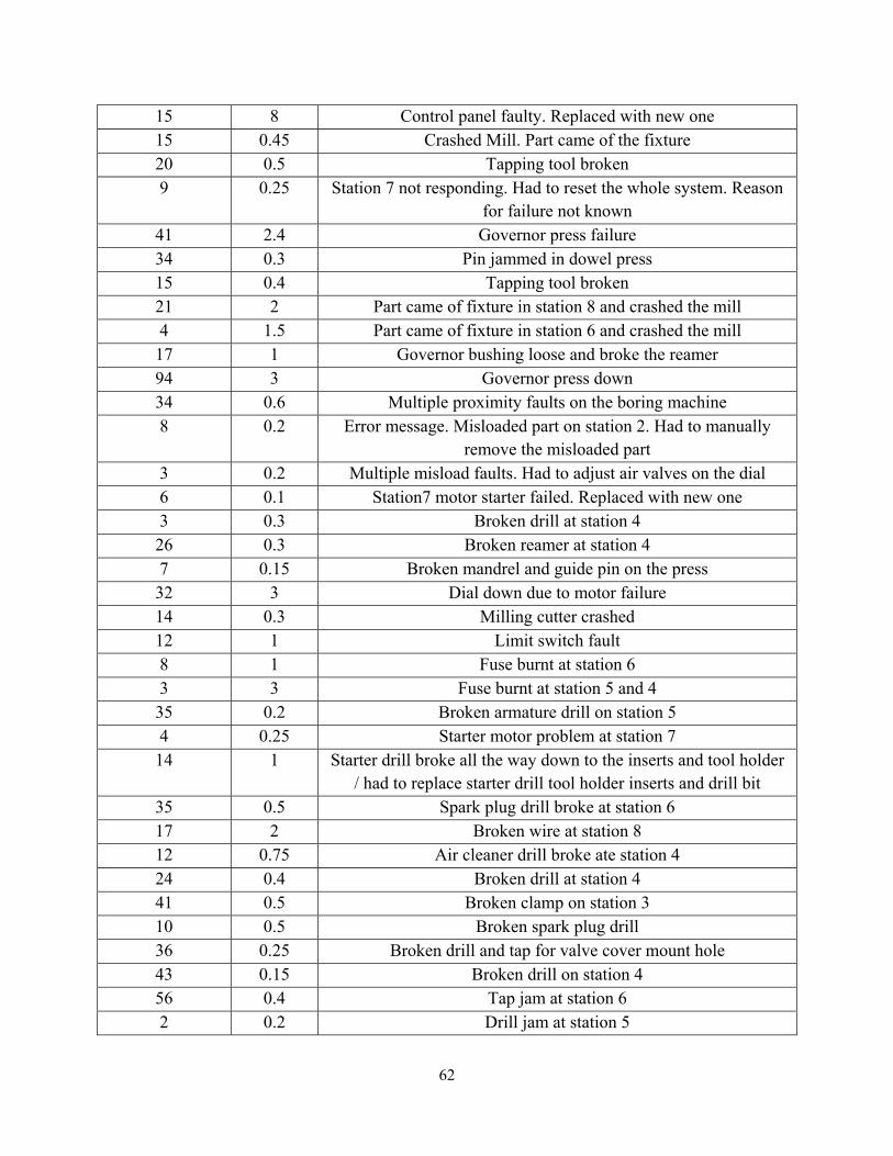
62
15 8 Control panel faulty. Replaced with new one 15 0.45 Crashed Mill. Part came of the fixture 20 0.5 Tapping tool broken 9 0.25 Station 7 not responding. Had to reset the whole system. Reason
for failure not known 41 2.4 Governor press failure 34 0.3 Pin jammed in dowel press 15 0.4 Tapping tool broken 21 2 Part came of fixture in station 8 and crashed the mill 4 1.5 Part came of fixture in station 6 and crashed the mill 17 1 Governor bushing loose and broke the reamer 94 3 Governor press down 34 0.6 Multiple proximity faults on the boring machine 8 0.2 Error message. Misloaded part on station 2. Had to manually
remove the misloaded part 3 0.2 Multiple misload faults. Had to adjust air valves on the dial 6 0.1 Station7 motor starter failed. Replaced with new one 3 0.3 Broken drill at station 4 26 0.3 Broken reamer at station 4 7 0.15 Broken mandrel and guide pin on the press 32 3 Dial down due to motor failure 14 0.3 Milling cutter crashed 12 1 Limit switch fault 8 1 Fuse burnt at station 6 3 3 Fuse burnt at station 5 and 4 35 0.2 Broken armature drill on station 5 4 0.25 Starter motor problem at station 7 14 1 Starter drill broke all the way down to the inserts and tool holder
/ had to replace starter drill tool holder inserts and drill bit 35 0.5 Spark plug drill broke at station 6 17 2 Broken wire at station 8 12 0.75 Air cleaner drill broke ate station 4 24 0.4 Broken drill at station 4 41 0.5 Broken clamp on station 3 10 0.5 Broken spark plug drill 36 0.25 Broken drill and tap for valve cover mount hole 43 0.15 Broken drill on station 4 56 0.4 Tap jam at station 6 2 0.2 Drill jam at station 5

63
25 0.2 Broken muffler mount tap on station 7 22 0.4 Broken drill on two spindle machine 61 0.4 Broken drill on station 4 75 3 Multiple tool breakage on Transfer line 26 0.2 Broken reamer on exhaust side 161 0.75 Broken wire in panel causing dial not to rotate 42 0.2 Broken drill on station 6 43 1 Broken drill and bushing on station 6 32 0.75 Fixture failed to clamp on station 2 24 3 Broken belt on the Transfer line 72 0.5 Fixture failed to clamp on station 2 27 0.2 Station 2 not moving 24 0.5 Broken oil drill drain on station 6 4 0.5 Crashed Mill on station 2 50 1.5 Transfer line dial crashed 42 0.5 Pneumatic valve failure 65 0.7 Taper jam at station 7
6.1 Identifying appropriate time between failures (TBF) distribution for the Transfer line
Form the recorded failure data of transfer line the Goodness of fit tests were conducted on
Minitab© statistical software. The results of the tests for the failure data from the transfer line
time between failure data are given below

64
Table 6.2: Minitab Goodness of fit tests for transfer line TBF
Distribution Anderson-Darling Statistic P value Normal 11.288 <0.005
Box-Cox Transformation 0.384 0.390 Lognormal 0.697 0.067
3-Parameter Lognormal 0.619 * Exponential 2.296 0.004
2-Parameter Exponential 2.372 <0.010 Weibull 0.713 0.063
3-Parameter Weibull 0.580 0.138 Smallest Extreme Value 16.729 <0.010 Largest Extreme Value 5.384 <0.010
Gamma 1.036 0.015 3-Parameter Gamma 0.845 *
Logistic 7.451 <0.005 Loglogistic 0.673 0.047
3-Parameter Loglogistic 0.728 *
From the above goodness of fit tests it is evident that none of the distributions except the Box-
Cox transformation provide the appropriate fit for the time between failure data of the transfer
lines. Box-Cox transformation could be used but it is not preferred in the field of reliability
engineering, because the resulting reliability estimates would correspond to the transformed data
not the true time between failures data. But it is essential to find an appropriate theoretical
distribution for estimating the reliability/availability measures.
In order to improve the distributional fit, it was decided to ascertain if the data contained outliers.
Some of the descriptive statistics from Minitab for the time between failure data from the
transfer line is shown in Table 6.3.

65
Table 6.3: Minitab Descriptive Statistics for Transfer Line TBF
The skewness value of 2.23 for the TBF data indicates that the TBF distribution is positively
skewed and there could be some extreme outliers present in the TBF data. Once the outliers are
identified and removed the TBF data could be again checked for goodness of fit and an
appropriate distribution to represent the TBF for the transfer line can be determined.
Extreme Outlier removal procedure:
The Boxplot is a useful graphical procedure to identify the outliers present in the data. A boxplot
is graphical measure of variability. Devore (2007) lists the prominent features that Boxplots
measure as (1) center, (2) spread, (3) the extent and nature of any departures from symmetry, and
(4) identification of outliers, observations that lie unusually far from the main body of the data.
The Boxplot of the time between failure data for the transfer line using Minitab is provided
below, where the outliers are represented by * symbol. The outliers are the points that 1.5
standard deviations outside the Interquartile range. From the Boxplot it is evident that there are
outliers only on the upper side of the interquartile range, due to large positive skewness.
Minitab Descriptive Statistics: Transfer Line TBF Sum of Variable Mean SE Mean TrMean StDev Variance CoefVar Sum Squares TBF 44.97 5.11 37.15 56.26 3165.11 125.10 5441.50 624523.25 N for Variable Minimum Q1 Median Q3 Maximum Range IQR Mode Mode TBF 0.50 8.50 25.00 55.50 260.00 259.50 47.00 3 7 Variable Skewness Kurtosis TBF 2.23 4.95

66
Figure 6.2: Minitab Boxplot for Transfer line TBF
By definition for the Boxplot any observation farther than 1.5 standard deviations from the
interquartile range is an outlier. An outlier is extreme if it is more than 3 standard deviations
from the interquartile range, and it is mild otherwise.
Unfortunately, Minitab does not differentiate mild outliers from extreme outliers in their Boxplot
and the outliers in the above Boxplot consist of both mild and extreme outliers. It is not
statistically justified to remove mild outliers from the data unless there are assignable causes. So
for the following analysis, only the extreme outliers were removed from the original TBF data. A
modified Boxplot with mild outliers differentiated from the extreme outliers is shown below.
250200150100500TBF
Boxplot of Transfer Line TBF
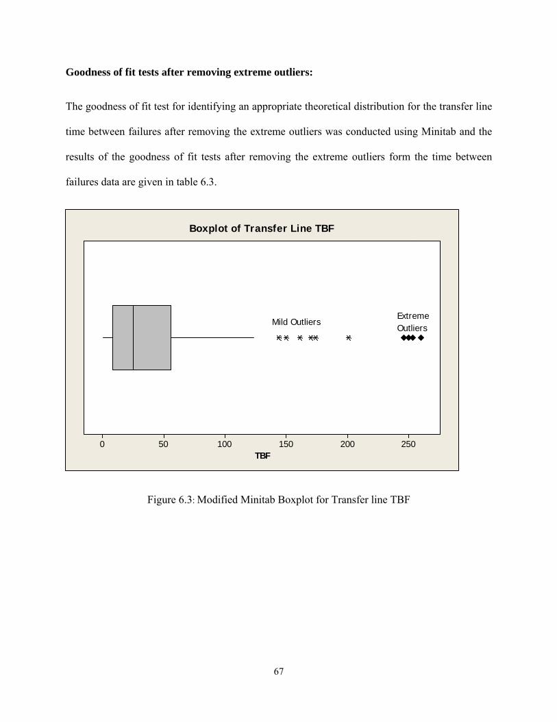
67
Goodness of fit tests after removing extreme outliers:
The goodness of fit test for identifying an appropriate theoretical distribution for the transfer line
time between failures after removing the extreme outliers was conducted using Minitab and the
results of the goodness of fit tests after removing the extreme outliers form the time between
failures data are given in table 6.3.
250200150100500TBF
OutliersExtreme
Mild Outliers
Boxplot of Transfer Line TBF
Figure 6.3: Modified Minitab Boxplot for Transfer line TBF

68
Table 6.4: Minitab Goodness of fit tests after removing extreme outliers
Distribution Anderson-Darling Statistic P value Normal 8.243 <0.005
Box-Cox Transformation 0.410 0.339 Lognormal 0.973 0.014
3-Parameter Lognormal 0.791 * Exponential 0.839 0.184
2-Parameter Exponential 0.892 0.144 Weibull 0.473 0.243
3-Parameter Weibull 0.401 0.387 Smallest Extreme Value 13.148 <0.010 Largest Extreme Value 3.618 <0.010
Gamma 0.576 0.171 3-Parameter Gamma 0.476 *
Logistic 5.501 <0.005 Loglogistic 0.910 0.010
3-Parameter Loglogistic 0.957 *
The above table 6.3 shows that the Weibull distribution has a sufficiently large P-value, which
implies that the Weibull can be an appropriate model for representing the time between failures
distribution of the transfer line. The three-parameter Weibull had a better fit than two-parameter
Weibull but it was not selected because the minimum life δ was too small.
The Goodness of fit test were once again conducted by removing both the mild and extreme
outliers (Mild = IQR±2σ; Extreme = IQR±3σ) from the time between failure data and the results
are shown below

69
Table 6.5: Minitab Goodness of fit tests after removing both mild and extreme outliers
Distribution Anderson-Darling Statistic P value Normal 6.075 <0.005
Box-Cox Transformation 0.466 0.249 Lognormal 1.268 <0.005
3-Parameter Lognormal 0.966 * Exponential 0.396 0.647
2-Parameter Exponential 0.410 >0.250 Weibull 0.400 >0.250
3-Parameter Weibull 0.367 0.451 Smallest Extreme Value 10.500 <0.010 Largest Extreme Value 2.525 <0.010
Gamma 0.423 >0.250 3-Parameter Gamma 0.378 *
Logistic 4.111 <0.005 Loglogistic 1.163 <0.005
3-Parameter Loglogistic 1.181 *
From the above results of the goodness of fit tests the Exponential distribution has an excellent
fit with a P-value of 0.647. Further the coefficient of variation with both the mild and extreme
outliers removed from the TBF data is 0.998783 which is approximately equal to 1 (the
theoretical CV for the Exponential density is 1) which confirms the fact that the TBF data when
both the mild and extreme outliers are removed is exponentially distributed.
Removing all the mild outliers from the sample data is a controversial approach in Reliability
Engineering the exponential distribution has too good a fit to be ignored when both the mild and
extreme outliers are removed. Therefore the reliability parameters were estimated for the
following two cases:

70
Case 1: The TBF has a Weibull distribution (Removing only the Extreme outliers)
Case 2: The TBF is exponentially distributed (Removing both mild and extreme outliers)
6.1.1 Case 1: The TBF has a Weibull distribution (Removing only the Extreme outliers):
Estimating the Weibull parameters β and θ using Maximum likelihood estimation (MLE):
The probability density function (pdf), f (t) of the 2-parameter Weibull distribution is given by
f(t) = 1 (t/ )t eββ− − θ
ββ
θ
This implies that the probability element of the ith failure time, ti, is given by
i(t / )1it e
β− θβ−β
βθ
dti and hence the LF (likelihood function) is given by
L( θ, β) = in
(t / )1i
i 1t e
β− θβ−β
=
βθ
∏ = n( )ββθ
×[n
1i
i 1tβ−
=∏ ] ×
ni
i 1(t / )
eβ
=− θ∑
(23)
Taking the natural log of (23) leads to
Ln L(θ,β) = n[ln(β) − β ln(θ)] + (β − 1)n
ii 1
ln(t )=∑ − ( / )
n
ii 1
t β
=θ∑ (24)
The partial derivative of the Log-likelihood, ln(θ, β), wrt θ is given by
∂[Ln L(θ, β)]/∂θ = − nβ/θ − ∂∂θ
[θ−βn
ii 1
(t )β
=∑ ] = − nβ/θ + β θ−β−1
n
ii 1
(t )β
=∑ Set to⎯⎯⎯→ 0 (25)
The solution to equation (25) is the MLE of θ which is given below.
θ̂ = ˆ1/n ˆ
ii 1
1 tn
ββ
=
⎡ ⎤⎢ ⎥⎢ ⎥⎣ ⎦
∑ (26)
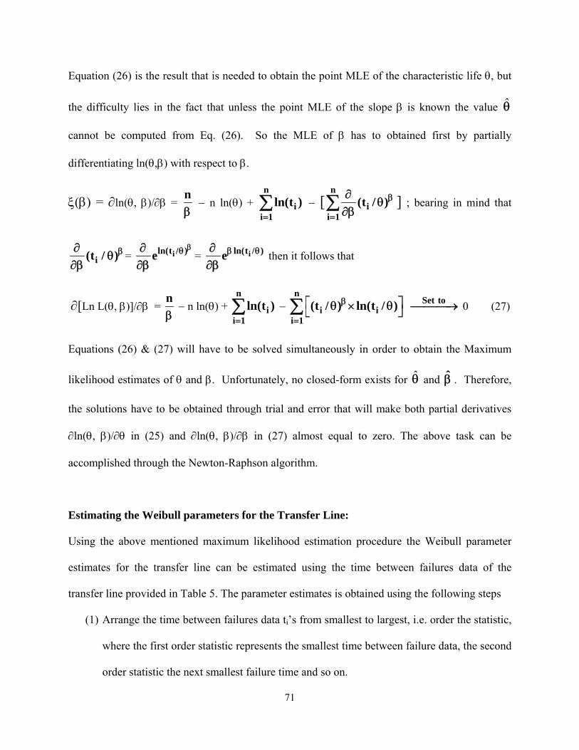
71
Equation (26) is the result that is needed to obtain the point MLE of the characteristic life θ, but
the difficulty lies in the fact that unless the point MLE of the slope β is known the value θ̂
cannot be computed from Eq. (26). So the MLE of β has to obtained first by partially
differentiating ln(θ,β) with respect to β.
ξ(β) = ∂ln(θ, β)/∂β = nβ
− n ln(θ) + n
ii 1
ln(t )=∑ − [
n
ii 1
(t / )β
=
∂θ
∂β∑ ] ; bearing in mind that
i(t / )β∂θ
∂β= iln(t / )e
βθ∂∂β
= iln(t / )eβ θ∂∂β
then it follows that
∂[Ln L(θ, β)]/∂β = nβ
− n ln(θ) + n
ii 1
ln(t )=∑ −
n
i ii 1
(t / ) ln(t / )β
=
⎡ ⎤θ × θ⎣ ⎦∑ Set to⎯⎯⎯→ 0 (27)
Equations (26) & (27) will have to be solved simultaneously in order to obtain the Maximum
likelihood estimates of θ and β. Unfortunately, no closed-form exists for θ̂ and β̂ . Therefore,
the solutions have to be obtained through trial and error that will make both partial derivatives
∂ln(θ, β)/∂θ in (25) and ∂ln(θ, β)/∂β in (27) almost equal to zero. The above task can be
accomplished through the Newton-Raphson algorithm.
Estimating the Weibull parameters for the Transfer Line:
Using the above mentioned maximum likelihood estimation procedure the Weibull parameter
estimates for the transfer line can be estimated using the time between failures data of the
transfer line provided in Table 5. The parameter estimates is obtained using the following steps
(1) Arrange the time between failures data ti’s from smallest to largest, i.e. order the statistic,
where the first order statistic represents the smallest time between failure data, the second
order statistic the next smallest failure time and so on.
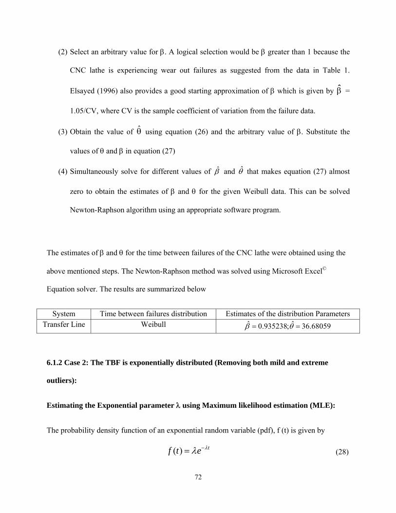
72
(2) Select an arbitrary value for β. A logical selection would be β greater than 1 because the
CNC lathe is experiencing wear out failures as suggested from the data in Table 1.
Elsayed (1996) also provides a good starting approximation of β which is given by β̂ =
1.05/CV, where CV is the sample coefficient of variation from the failure data.
(3) Obtain the value of θ̂ using equation (26) and the arbitrary value of β. Substitute the
values of θ and β in equation (27)
(4) Simultaneously solve for different values of β̂ and θ̂ that makes equation (27) almost
zero to obtain the estimates of β and θ for the given Weibull data. This can be solved
Newton-Raphson algorithm using an appropriate software program.
The estimates of β and θ for the time between failures of the CNC lathe were obtained using the
above mentioned steps. The Newton-Raphson method was solved using Microsoft Excel©
Equation solver. The results are summarized below
System Time between failures distribution Estimates of the distribution Parameters Transfer Line Weibull ˆ ˆ0.935238; 36.68059β θ= =
6.1.2 Case 2: The TBF is exponentially distributed (Removing both mild and extreme
outliers):
Estimating the Exponential parameter λ using Maximum likelihood estimation (MLE):
The probability density function of an exponential random variable (pdf), f (t) is given by
( ) tf t e λλ −= (28)

73
This implies that the probability element of the ith failure time, ti, is given by ite λλ − dti and
hence the likelihood function is given by
1
( ) i
nt
i
L e λλ λ −
=
= ∏
1( )
n
ii
tnL e
λ
λ λ =
− ∑=
Taking natural logarithm on both sides
1ln[ ( )] ln[ ]
n
ii
tnL e
λ
λ λ =
− ∑=
1ln[ ( )] ln( )
n
ii
L n tλ λ λ=
= − ∑
Taking derivative with respect to λ
1[ln( ( ))]
n
ii
nL tλλ λ =
∂= −
∂ ∑ Set to⎯⎯⎯→ 0
1
ˆn
ii
n
tλ
=
=
∑ (29)
Equation (29) gives the maximum likelihood estimate for the exponential distribution with
failure rate λ. So the failure rate λ for the Transfer line can be estimated using the time between
failures data of Table 5. From the time between failures data from table 5 and using equation
(29) the failure rate λ for Transfer line is estimated as
System Time between failures distribution Estimates of the distribution ParametersTransfer Line Exponential λ̂ =0.030323 per hour
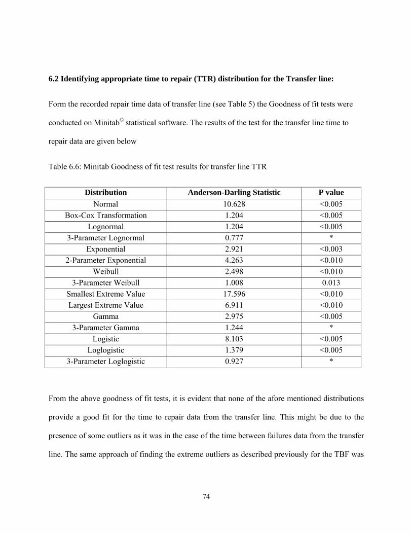
74
6.2 Identifying appropriate time to repair (TTR) distribution for the Transfer line:
Form the recorded repair time data of transfer line (see Table 5) the Goodness of fit tests were
conducted on Minitab© statistical software. The results of the test for the transfer line time to
repair data are given below
Table 6.6: Minitab Goodness of fit test results for transfer line TTR
Distribution Anderson-Darling Statistic P value Normal 10.628 <0.005
Box-Cox Transformation 1.204 <0.005 Lognormal 1.204 <0.005
3-Parameter Lognormal 0.777 * Exponential 2.921 <0.003
2-Parameter Exponential 4.263 <0.010 Weibull 2.498 <0.010
3-Parameter Weibull 1.008 0.013 Smallest Extreme Value 17.596 <0.010 Largest Extreme Value 6.911 <0.010
Gamma 2.975 <0.005 3-Parameter Gamma 1.244 *
Logistic 8.103 <0.005 Loglogistic 1.379 <0.005
3-Parameter Loglogistic 0.927 *
From the above goodness of fit tests, it is evident that none of the afore mentioned distributions
provide a good fit for the time to repair data from the transfer line. This might be due to the
presence of some outliers as it was in the case of the time between failures data from the transfer
line. The same approach of finding the extreme outliers as described previously for the TBF was

75
employed. Some of the descriptive statistics from Minitab for the time to repair data from the
transfer line is shown below
Figure 6.4 Minitab descriptive statistics for Transfer line TTR
The above descriptive statistics indicates that the skewness value for the TTR data is 2.71, which
indicates that the data is positively skewed and indicates the presence of some outliers in the
TTR data. The Boxplot of the TTR data is shown in figure 6.4.
Minitab Descriptive Statistics: Transfer Line TTR Sum of Variable Mean SE Mean TrMean StDev Variance CoefVar Sum Squares TTR 1.001 0.111 0.850 1.218 1.485 121.68 121.170 299.503 N for Variable Minimum Q1 Median Q3 Maximum Range IQR Mode Mode TTR 0.080 0.250 0.500 1.250 8.000 7.920 1.000 0.2 14 Variable Skewness Kurtosis TTR 2.71 10.28

76
9876543210TTR
Boxplot of Transfer Line TTR
Figure 6.4: Minitab Boxplot for transfer line TTR
As mentioned previously Minitab plots outliers 1.5 standard deviations outside the interquartile
range which includes both mild and extreme outliers. A modified Boxplot indicating both the
mild (IQR±1.5σ) and extreme outliers (IQR±3σ) is shown below. To be more conservative and
avoid trimming more data points IQR±2σ can be termed as mild outliers and IQR±3σ as extreme
outliers.

77
9876543210TTR
Boxplot of Transfer L ine TTR
Extreme OutliersM ild Outliers
Figure 6.5: Modified Minitab Boxplot for transfer line TTR
Removing the extreme outliers and conducting the Goodness of fit again in Minitab yields the
following results

78
Table 6.7: Minitab Goodness of fit tests for Transfer line TTR after removing extreme outliers
Distribution Anderson-Darling Statistic P value Normal 9.514 <0.005
Box-Cox Transformation 1.299 <0.005 Lognormal 1.299 <0.005
3-Parameter Lognormal 0.915 * Exponential 2.377 <0.004
2-Parameter Exponential 3.102 <0.010 Weibull 2.534 <0.010
3-Parameter Weibull 1.090 0.008 Smallest Extreme Value 12.281 <0.010 Largest Extreme Value 6.557 <0.010
Gamma 2.843 <0.005 3-Parameter Gamma 1.210 *
Logistic 7.806 <0.005 Loglogistic 1.456 <0.005
3-Parameter Loglogistic 1.028 *
After removing the extreme outliers, the data still does not fit into any statistical distribution. The
goodness of fit test was conducted again by removing both mild and extreme outliers and the
results are provided below.

79
Table 6.8: Minitab Goodness of fit tests for Transfer line TTR after removing mild and extreme
outliers
Distribution Anderson-Darling Statistic P value Normal 7.421 <0.005
Box-Cox Transformation 1.071 0.008 Lognormal 1.299 0.008
3-Parameter Lognormal 0.874 * Exponential 2.194 0.006
2-Parameter Exponential 1.359 0.040 Weibull 2.138 <0.010
3-Parameter Weibull 0.954 0.018 Smallest Extreme Value 10.186 <0.010 Largest Extreme Value 4.686 <0.010
Gamma 2.191 <0.005 3-Parameter Gamma 0.982 *
Logistic 6.008 <0.005 Loglogistic 1.231 <0.005
3-Parameter Loglogistic 0.978 *
Even after removing mild and extreme outliers the time to repair data still does not follow any of
the above mentioned theoretical distribution. In order to find a theoretical distribution for the
time to repair data to estimate the reliability/availability measures, another approach is to
compare the Skewness (the third standardized central moment) and Kurtosis (fourth standardized
central moment - 3) from the sample data to the skewness and kurtosis of known theoretical
distributions. The skewness and the kurtosis value of the TTR data from the above Minitab
descriptive statistics are 2.71 and 10.28 respectively. The derived skewness and kurtosis of some
of the theoretical distributions are given below.
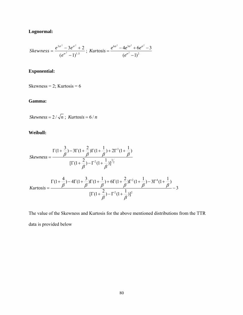
80
Lognormal:
2 2
2
3
1.5
3 2( 1)
e eSkewnesse
σ σ
σ
− +=
−;
2 2 2
2
6 3
2
4 6 3( 1)
e e eKurtosise
σ σ σ
σ
− + −=
−
Exponential:
Skewness = 2; Kurtosis = 6
Gamma:
2 /Skewness n= ; 6 /Kurtosis n=
Weibull:
3
32 2
3 2 1 1(1 ) 3 (1 ) (1 ) 2 (1 )
2 1[ (1 ) (1 )]Skewness β β β β
β β
Γ + − Γ + Γ + + Γ +=
Γ + − Γ +
2 4
2 2
4 3 1 2 1 1(1 ) 4 (1 ) (1 ) 6 (1 ) (1 ) 3 (1 )32 1[ (1 ) (1 )]
Kurtosis β β β β β β
β β
Γ + − Γ + Γ + + Γ + Γ + − Γ += −
Γ + − Γ +
The value of the Skewness and Kurtosis for the above mentioned distributions from the TTR
data is provided below

81
Distribution Skewness Kurtosis Lognormal 11.84974627 603.8606093 Exponential 2 6
Gamma 1.990232029 5.941535293 Weibull** 3.017207731 10.13499102
**The value of β was computed for the TTR data from Table 6.1 using equations (26) and (27)
From the above table the theoretical Skewness and Kurtosis value of the Weibull distribution is
the only one close to the skewness and kurtosis value from the TTR data in table 5 (2.71 and
10.27 respectively). Even though Weibull is a flexible distribution, it is impractical to find a
value of β for which Skewness and Kurtosis will equal 2.71 and 10.27 respectively. But it is
possible to find a value of β for which the theoretical value of skewness value would equal
2.7114. Through trial and error, the β̂ value for which the theoretical Weibull skewness is equal
to 2.7114 is computed to be 0.81923.
Substituting β̂ =0.81923 equation (26) gives the value θ̂ = 0.907962.
System Time to repair distribution Estimates of the distribution ParametersTransfer Line Weibull β̂ =0.81923; θ̂ = 0.907962

82
6.3 Estimating Reliability of the Transfer Line:
6.3.1 Case 1: Using Weibull TBF Distribution:
The time between failures for the transfer line follows Weibull distribution (see Table 5). The
probability density function f(t) of the 2 parameter Weibull distribution is given by
1 ( / )( ) tf t t eββ θ
β
βθ
− −=
Using (12)
1 ( / )( ) tTRANSFERLINE
t
R t t e dtββ θ
β
βθ
∞− −= ∫
Solving the above expression through integration by parts yields
( / )( ) t
TRANSFERLINER t eβθ−= (30)
Substituting the values of θ = 36.68059 and β = 0.935238 obtained earlier for transfer line time
between failures through maximum likelihood estimation into equation (30) yields
(160 ) 0.018966TRANSFERLINER hours =
The mean time between failures for the CNC lathe can be estimated from equation (30)
( / )
0
tTRANSFERLINEMTBF e dt
βθ∞
−= ∫
Making the transformation x = (t/θ)β in the above integral results in
1/ 1
0
1 ( )xTRANSFERLINEMTBF e x dxβ βθ
β
∞− −= ∫

83
(1/ ) 1
0
1 xx e dxβθβ
∞− −= ∫
By definition a gamma random variable ( )nΓ is defined by
1
0
( ) n xn x e dx∞
− −Γ = ∫
Using the above fact, the MTBF can be rewritten as
1 (1/ )TRANSFERLINEMTBF θ ββ
= Γ
Using the property of the gamma function, ( ) ( 1)n n nΓ = Γ + the MTBF equation becomes
(1 1/ )TRANSFERLINEMTBF θ β= ×Γ + (31)
Substituting the values of θ = 36.68059 and β = 0.935238 obtained earlier for CNC lathe time
between failures through maximum likelihood estimation into equation (31) yields
37.82796TRANSFERLINEMTBF hours= (32)
As mentioned previously the time to repair (TTR) data follows a Weibull distribution. Using the
previously obtained value of β = 0.81923 in equation (31) yields
1.01183TRANSFERLINEMTTR hours= (33)
By definition the instantaneous availability is defined as
( )
UPTIMEAvailabilityUPTIME DOWNTIME
=+
(34)
Mathematically that is equivalent to

84
( )
MTBFAvailabilityMTBF MTTR
=+
(35)
Substituting (32) and (33) in (35) gives the availability of transfer line
0.970090401TRANSFERLINEAvailability =
6.3.2 Case 2: Using Exponential TBF distribution:
The probability density function f(t) of the Exponential distribution is given by
( ) tf t e λλ −=
Using (12)
( ) xTRANSFERLINE
t
R t e dxλλ∞
−= ∫
Solving the above integral results in
( ) t
TRANSFERLINER t e λ−= (36)
Substituting the values of λ = 0.030323 obtained earlier for the transfer line time between
failures through maximum likelihood estimation into equation (36) yields
(160 ) 0.007815TRANSFERLINER hours =
Using equation (15)
0
tTRANSFERLINEMTBF e dtλ
∞−= ∫
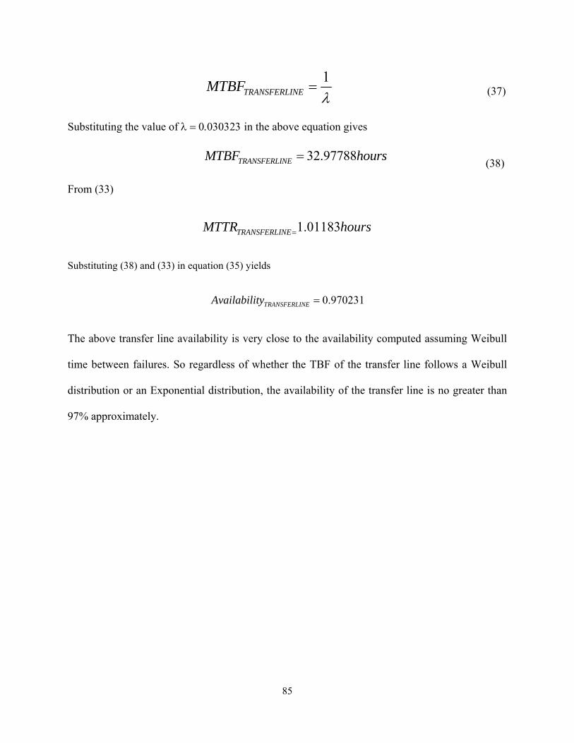
85
1TRANSFERLINEMTBF
λ= (37)
Substituting the value of λ = 0.030323 in the above equation gives
32.97788TRANSFERLINEMTBF hours= (38)
From (33)
1.01183TRANSFERLINEMTTR hours=
Substituting (38) and (33) in equation (35) yields
0.970231TRANSFERLINEAvailability =
The above transfer line availability is very close to the availability computed assuming Weibull
time between failures. So regardless of whether the TBF of the transfer line follows a Weibull
distribution or an Exponential distribution, the availability of the transfer line is no greater than
97% approximately.

86
CHAPTER 7
Results
The Weibull distribution was found suitable in most of the cases to represent the time between
failures distribution of CNC machines used in manufacturing cell. Goodness of fit tests was used
to identify the appropriate distributions for time between failures of CNC machines used in the
manufacturing cell. When the data contained outliers, Goodness of fit tests failed to identify an
appropriate distribution to represent time between failures of Transfer Lines. To identify an
appropriate time between failure distributions for transfer line, both mild and extreme outliers in
the data was identified and removed. Goodness of fit test was conducted for two cases –
removing only mild outliers and removing both mild and extreme outliers. Weibull distribution
had a good fit after removing the mild outliers from transfer line TBF data and exponential
distribution gave an excellent fit after removing both mild and extreme outliers from the Transfer
Line TBF data. Reliability measures were calculated for both cases and the reliability measures
was not significantly different for the two cases considered. Goodness of fit test failed to
identify an appropriate distribution, even after removing mild and extreme outliers from the time
to repair data of the Transfer Line. Skewness and Kurtosis values were used identify an
appropriate time to repair distribution. Weibull distribution was found suitable to represent the
time to repair distribution of the Transfer Line.
After identifying the appropriate time between failures and time to repair distributions, the
necessary reliability measures were estimated for manufacturing cell and transfer line. Once the
necessary reliability measures were obtained, availability of manufacturing cell and transfer line

87
was determined. The crankshaft manufacturing cell considered in this thesis was available
99.76% of the time and the Transfer Line was available 97.06% of the time.

88
CHAPTER 8
Conclusion
The statistical reliability model proposed in this thesis is simple and could be employed by
manufacturing organizations to estimate availability and MTBF of their machine tools/transfer
lines. Collecting field failure data is essential for assessment and improvement of system
reliability. Selecting an appropriate distribution for failure data is essential in predicting the
reliability measures. The results of this thesis shows that the Weibull distribution could be used
most of the time to represent time between failures and repair time distribution of machine tools
and transfer lines. Once the time between failures distribution is identified, all the other
reliability/availability measures could be derived using suitable statistical estimation techniques.
Availability is a function of MTBF and MTTR. To increase availability the MTBF should be
increased and/or the MTTR should be reduced. MTBF can be increased by improving the
reliability of the components/system hence reducing frequency of failures whereas MTTR can be
reduced by proper maintenance techniques, proper training and by employing
preventive/predictive maintenance.
To improve the reliability of manufacturing systems, the critical components affecting the
system reliability should be identified and failure mode and effect analysis (FMEA) should be
conducted for each of these critical components. Field failure data should be collected for each of
the failure modes. With the above information, periodic replacement and preventive & predictive
maintenance can be scheduled to improve the system reliability. This proposed method is
effective in improving system reliability, but the above methodology could be very complicated

89
to implement in transfer lines and flexible manufacturing systems since the number of critical
components and their failure modes is quite large.
Preventive maintenance can reduce the frequency of failures, but it is often difficult to determine
the proper maintenance interval. Preventive maintenance can be termed as scheduled downtime.
Preventive maintenance performed too frequently can actually decrease availability. Whenever
the complexity of the system increases, the complexity of maintainability along with the cost
involved in maintenance also increases. Even though the operations of the transfer lines and
flexible manufacturing systems are entirely automatic, the maintenance of those complex
systems is still completely manual. Unlike manufacturing cells in which operators can perform
maintenance and basic repairs, the transfer line requires specialized maintenance personnel for
repair and routine maintenance.
Manufacturing cells could be considered more reliable than transfer lines, but it is unfair to
compare the reliability of manufacturing cell with that of transfer lines because the transfer line
has much more components/stations than manufacturing cells. But from a maintainability
standpoint, manufacturing cells provide the advantage of having simple CNC machine tools
which are much easier to maintain and repair than transfer lines. In addition, operators in
manufacturing cell can perform basic repair operations on machine tools in manufacturing cell
whereas the transfer line requires trained maintenance technicians to perform repairs on transfer
lines. In conclusion, an increase in automation requires higher reliability and maintainability
requirements to increase manufacturing uptime.
90
References:
1. Abernethy, R., 2010, The New Weibull Handbook, Abernethy publications.
2. Adamyan, A , He, D, 2002 Analysis of sequential failures for assessment of reliability and
safety of manufacturing systems, Reliability Engineering & System Safety, Volume 76, Issue
3.
3. Agarwal, A., Sarkis, J., 1998., A review and analysis of comparative performance studies on
functional and cellular manufacturing layouts, Computers & Industrial Engineering, Volume
34, Issue 1.
4. Askin, R.G., Standridge, C.R., 1993, Modeling and Analysis of Manufacturing Systems,
John Wiley.
5. Askin, R.G., Zhou, M., 1998, Formation of general GT cells: an operation-based approach,
Computers & Industrial Engineering, Volume 34, Issue 1.
6. Balanchard, B, 1998, Systems Engineering and Analysis, Prentice Hall.
7. Black. J T, Hunter. S, 2003, Lean Manufacturing Systems and Cell Design, Society of
Manufacturing Engineers.
8. Black. J T., Phillips. D.T., In press, Lean Engineering, Society of Manufacturing Engineers.
9. Curry, G.L., Feldman, R.M., Manufacturing Systems Modeling and Analysis, 2010,
Springer.
10. Das, K. Lashkari, R.S, Sengupta, S., 2007, Reliability consideration in the design and
analysis of cellular manufacturing systems, International Journal of Production Economics,
Volume 105, Issue 1.
11. Dennis, P., 2002, Lean Production Simplified, Productivity Press.
91
12. Devore, J. L., 2007, Probability and Statistics for Engineering and the Sciences, CENGAGE
Learning.
13. Dhillon, B.S, 1983, Reliability Engineering in Systems Design and Operation, Van Nostrand
Reinhold.
14. Diallo, M., Pierreval., Quilliot, A., 2001, Manufacturing cells design with flexible routing
capability in presence of unreliable machines., International Journal of Production
Economics, Volume 74, Issues 1-3
15. Ebeling, C.E, 1997, An Introduction to Reliability and Maintainability Engineering,
Waveland Press.
16. Elsayed, E.A., 1996, Reliability Engineering, Addison Wesley Longman.
17. Greshwin, S. B., 1993, Manufacturing Systems Engineering, Prentice Hall.
18. Groover, M.P., 2000, Automation, Production Systems and Computer Integrated
Manufacturing, Prentice Hall.
19. Hon, K.K.B., 2005, Performance and Evaluation of Manufacturing Systems, CIRP Annals of
Manufacturing Technology, Volume 54, Issue 2.
20. Hunter, S. L., 2002, Ergonomic evaluation of manufacturing system designs, Journal of
Manufacturing Systems, Volume 20, Issue 6.
21. Irani, S.A., Handbook of cellular manufacturing systems, 1999, John Wiley.
22. Jeon, G., Broering, M., Parsaei, H.R., Wong, J.P., 1998, Part family formation based on
alternative routes during machine failure, Computers & Industrial Engineering, Volume 35,
Issues 1-2
23. Kapur, K.C., Lamberson L.R, 1977, Reliability in Engineering Design, John Wiley.

92
24. Kavusturucu, A., Gupta, S.M., 1999, Manufacturing systems with machine vacations,
arbitrary topology and finite buffers., International Journal of Production Economics, Volume
58, Issue 1
25. Lawless, J.F., 2002, Statistical models and methods for lifetime data, Wiley – Interscience.
26. Logendran, R., Talkington, D., 1997, Analysis of cellular and functional manufacturing
systems in the presence of machine breakdown, International Journal of Production
Economics, Volume 53, Issue 3, 4.
27. Nakajima, S., 1988, Introduction to TPM: Total Productive Maintenance, Productivity Press.
28. O’Connor, P., 2002, Practical Reliability Engineering, John Wiley.
29. Savsar, M., 2000, Reliability analysis of a flexible manufacturing cell, Reliability
Engineering & System Safety, Volume 67, Issue 2.
30. Seifoddini, H., Djassemi, M., 2001, The effect of reliability consideration on the application
of quality index, Computers & Industrial Engineering, Volume 40, Issues 1-2.
31. The Dictionary of Engineering, 2003, McGraw-Hill Professional
32. Vineyard, M. Gyampah, K.A. Meredith, J.R, 1999, Failure rate distributions for flexible
manufacturing systems: An empirical study, European Journal of Operational Research,
Volume 116, Issue 1.
33. Wang, Y., Yazhou, J., Yi, S., 1999, Failure probabilistic model of CNC lathes, Reliability
Engineering and System Saftey, Volume 65, Issue 3.
34. Wemmerlov, U., Hyer, N.L., 1986, Procedures for the part family/machine group
identification problem in cellular manufacturing, Journal of Operations Management,
Volume 6, Issue 2.

93
35. Yazhou, J., Wang, M., Zhixn, J., Probability distribution of machining center failures,
Reliability Engineering and System Saftey, Volume 50, Issue 2.

94
APPENDIX
Lean tools and manufacturing waste
The 8 Deadly Manufacturing Waste:
(1) Defects – Producing products that do not meet customer or design specifications. Defects
may lead to rework or scrap, which represents the waste of material, time and energy
involved in making and correcting defects.
(2) Overproduction – Producing products that are not required by the customers yet.
Considered the worst manufacturing waste as overproduction leads to the waste of inventory,
which has to be stored, accounted and protected.
(3) Waiting – The waste of waiting for materials, waiting for machines to process the part and
waiting for broken machine to get repaired. It is considered a waste because the operator or
employee is still paid for the period of time spent in waiting.
(4) Not utilizing people – Dennis (2002) defines wasted talent as disconnects within or between
the company and its customers and suppliers. These inhibit the flow of knowledge, ideas, and
creativity, creating frustration and missed opportunities.
(5) Excessive Transportation – Waste of excessive transportation caused by poor layout/facility
design, keeping processes far away from each other, overly large equipment. This waste
represents inefficient use of factory space.
(6) Excessive Inventory – The waste of excess inventory is related to keeping unnecessary raw
materials, WIP and finished products. Excess inventory has to be stored, accounted and
protected which requires space, energy, money and labor.

95
(7) Excessive Motion – Excessive motion represents a loss of productivity due to poor
occupational ergonomics. Quality and productivity of operator is reduced when there is
awkward postures and repetitive motion involved in the task.
(8) Extra processing – This waste is related to doing more than what the customers desire. This
is often caused by loss of information flow between marketing, design, engineering, and
production department.
Lean tools:
(1) Manufacturing cells – See section 3.1, page 17
(2) Pull system/Kanban – To produce an item only when the customer asks for it. This
production control is achieved through Kanban cards and carts, which avoids production in
the upstream processes until the downstream process requires it.
(3) Poka–yokes – Defect prevention devices built within the equipment which prevents the
operators from producing defects/ human errors.
(4) Quick changeover – A structured methodology (pioneered by Shigeo Shingo) of converting
internal elements (processes that can be performed only when machine is stopped) into
external elements (processes which can be performed when equipment is running) to reduce
setup/changeover time.
(5) JIDOKA – Sensible automation of separating operator’s task from machine task, which
enables the operator to leave the machine when running, to perform other value added tasks.
(6) Value stream mapping – A high level process mapping used to identify the non value added
activities in all the steps required to bring a product to a customer.
(7) 5S – A system of workplace standardization and housekeeping aimed at reducing the non-
value added activities in the workplace.

96
(8) Total productive maintenance (TPM) – Methodology to increase overall equipment
effectiveness and achieve zero downtime by measuring the six big losses, prioritizing
problems, and solving the problem through autonomous maintenance.


