

VHDL- IMPLEMENTATION 0F LMS BASED ADAPTIVE NOISE CANCELLER Department of EXTC
Dr. Bhausaheb Nandurkar College Of Engineering and Technology Page 1
CHAPTER 1
INTRODUCTION
The FIR filter computations play an important role in the DSP systems. The FIR filtering is
a convolution operation which can be viewed as the weighted summation of the input
sequences. The large amount of multiply and accumulate operations attracts many researchers
to study this issue. The FIR Filter consists of shifters, adders, and multipliers. These
constitutes can be chosen on the demand of the designer. As the FIR filter alone can’t solve
the problem of non stationary noise, there is a a great need for making the filter adaptive.
There are number of possible algorithms available for designing of adaptive filter. One of the
most popular adaptive algorithms available in the literature is the stochastic gradient
algorithm also called least-mean-square (LMS). Its popularity comes from the fact that it is
very simple to implement. As a consequence, the LMS algorithm is widely used in many
applications.
Least–Mean - Square (LMS) adaptive filter is the main component of many
communication systems; traditionally, such adaptive filters are implemented in Digital Signal
Processors (DSPs). Sometimes, they are implemented in ASICs, where performance is the
key requirement. However, many high-performance DSP systems, including LMS adaptive
filters, may be implemented using Field Programmable Gate Arrays (FPGAs) due to some of
their attractive advantages. Such advantages include flexibility and programmability but most
of all availability of tens to hundreds of hardware multipliers available on a chip. The LMS
adaptive filter enjoys a number of advantages over other adaptive algorithms, such as robust
behavior when implemented in finite-precision hardware, well understood convergence
behavior and computational simplicity for most situations as compared to least square
VHDL- IMPLEMENTATION 0F LMS BASED ADAPTIVE NOISE CANCELLER Department of EXTC
Dr. Bhausaheb Nandurkar College Of Engineering and Technology Page 2
methods Identifying an unknown system has been a central issue in various application areas
such as channel equalization, echo cancellation in communication networks and
teleconferencing etc. Identification is the procedure of specifying the unknown model in
terms of the available experimental evidence, that is a set of measurements of the input output
desired response signals and an appropriately error that is optimized with respect to unknown
model parameters. Adaptive identification refers to a particular procedure where we learn
more about the model as each new pair of measurements is received and we update the
knowledge to incorporate the newly received information.
The Least Mean Square (LMS) adaptive filter is a simple well behaved
algorithm which is commonly used in applications where a system has to adapt to its
environment. Architectures are examined in terms of the following criteria: speed, power
consumption and FPGA resource usage. Modern FPGAs contain many resources that support
DSP applications .These resources are implemented in the FPGA fabric and optimized for
high performance and low power consumption. This project proposes a VHDL
implementation of a Least Mean Square (LMS) adaptive algorithm. The good convergence of
LMS algorithm has made us to choose it. It also has good stability. Adaptive filtering
constitutes one of the core technologies in digital signal processing and finds numerous
application areas in science as well as in industry. In this project LMS algorithm is used to
reduce the error at the output of the system. A VHDL implementation is developed for a
LMS adaptive filter. It has been proven that LMS Algorithm has good behavior.
The method used to cancel the noise signal is known as adaptive filtering.
Adaptive filters are dynamic filters which iteratively alter their characteristics in order to
achieve an optimal desired output. An adaptive filter algorithmically alters its parameters in
order to minimize a function of the difference between the desired output d(n) and its actual
output y(n) . This function is known as the objective function of the adaptive algorithm.
VHDL- IMPLEMENTATION 0F LMS BASED ADAPTIVE NOISE CANCELLER Department of EXTC
Dr. Bhausaheb Nandurkar College Of Engineering and Technology Page 3
USED TOOLS: XILINX 13.
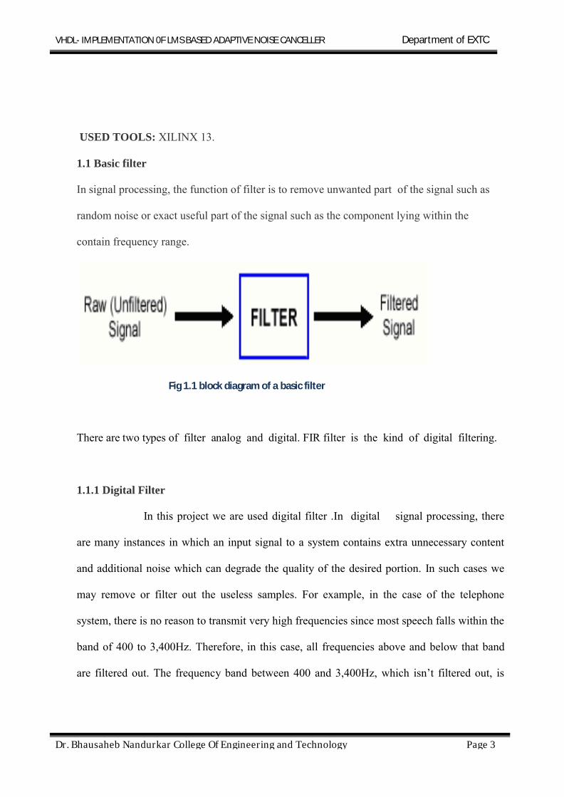
1.1 Basic filter
In signal processing, the function of filter is to remove unwanted part of the signal such as
random noise or exact useful part of the signal such as the component lying within the
contain frequency range.
Fig 1.1 block diagram of a basic filter
There are two types of filter analog and digital. FIR filter is the kind of digital filtering.
1.1.1 Digital Filter
In this project we are used digital filter .In digital signal processing, there
are many instances in which an input signal to a system contains extra unnecessary content
and additional noise which can degrade the quality of the desired portion. In such cases we
may remove or filter out the useless samples. For example, in the case of the telephone
system, there is no reason to transmit very high frequencies since most speech falls within the
band of 400 to 3,400Hz. Therefore, in this case, all frequencies above and below that band
are filtered out. The frequency band between 400 and 3,400Hz, which isn’t filtered out, is

VHDL- IMPLEMENTATION 0F LMS BASED ADAPTIVE NOISE CANCELLER Department of EXTC
Dr. Bhausaheb Nandurkar College Of Engineering and Technology Page 4
known as the pass band, and the frequency band that is blocked out is known as the stop
band.
1.1.2 Digital Filter Types
There are two basic types of digital filters, Finite Impulse Response (FIR) and Infinite
Impulse response (IIR) filters. The general form of the digital filter difference equation is
y(n)= ai x(n − i)- bi y(n − i)Where, y(n) is the current filter output, the y(n-i)’s are previous filter outputs, the
x(n-i)’s are current or previous filter inputs, the ai are the filter field forward coefficients
corresponding to the zeros of the filter, the bi are the filters feedback coefficients
corresponding to the poles of the filter, and N is the filters order.
FIR, Finite Impulse Response filters are one of the primary types of filters used in
Digital Signal Processing. FIR filters are said to be finite because they do not have any
feedback. Therefore, if we send an impulse through the system(a single spike) then the output
will invariably become zero as soon as the impulse runs through the filter.
IIR filters have one or more nonzero feedback coefficients. That is as a result of the
feedback term, if the filters has one or more poles, once the filter has been excited with an
impulse there is always an output. FIR filters have no nonzero feedback coefficients. That is,
the filter has only zeros, and once it has been excited with an impulse, the output is present
for only a finite (N) number of computational cycles.
Because an IIR uses both a feed- forward polynomial (zeros as the root) and a feed
backward. Like analog filters with poles, an IIR filter usually has nonlinear phase

VHDL- IMPLEMENTATION 0F LMS BASED ADAPTIVE NOISE CANCELLER Department of EXTC
Dr. Bhausaheb Nandurkar College Of Engineering and Technology Page 5
characteristics. Also, the feedback loop makes IIR filter difficult to use in adaptive filter
applications.
Due to its all zero structure, the FIR filter has a linear phase response when the filters
coefficients are symmetric, as is the case in most standard filtering applications. FIR
implementation noise characteristics are easy to model, especially if no intermediate
truncation is used. In this common implementation, the noise floor is at -6.02 B + 6.02 log2N
dB, where B is the number of actual bits used in the filters coefficient quantization and N is
again the filter order. That’s why most intarsia filter ICs has more coefficient bits than data
bits.
An IIR filters poles may be close to or outside the unit circle in the Z plane. This
means an IIR filter may have stability problems, especially after quantization is applied. An
FIR filter is always stable.
A digital filter is characterized in terms of difference equations. There are two types
of digital filters, they are non-recursive, and recursive filters which are characterized based
on their responses.
The response of a non-recursive filter at any instant depends on the present, past future values
of the input. At any specific instant nT. The response is of the form
Y(nT) = f(….,x(nT-T), x(nT), x(nT+T)…. )
Assuming linearity and time- invariance y(nT) can be expressed as
y( ) = ai x(nT − iT)Where ‘ai’s represents constants.
Now assuming causality for the filter we have
VHDL- IMPLEMENTATION 0F LMS BASED ADAPTIVE NOISE CANCELLER Department of EXTC
Dr. Bhausaheb Nandurkar College Of Engineering and Technology Page 6
a-1 = a-2 =….=0
In addition, assuming ai=0 for i > N the response can be written as Nth order linear difference
equation given as:
y( ) = ai x(nT − iT)Such a linear, time invariant, causal, non-recursive filter represented as Nth order linear
difference equation is called the Finite Impulse Response (FIR) filter.
When a unit impulse is defined as
δ(nT)= 1 for n=0
0 for n≠ 0
Is applied to the system described by equation, then the response, which is nothing but
the impulse response h(nT) is given as
h(nT) = ai δ(nT − iT)From the above equation it can be inferred that the impulse response is finite and from the
property of the impulse function we can see the constants s are nothing but the samples of the
impulse response. That means
h(0) = a0 ,h(T) = a1……h(nT) = an
these constants are called the filter coefficients. They determine the type of the filter, whether
it is Low-pass, or High-pass. Thus in filter design it is always important to find the filter
coefficients which mostly approximate the desired response.
In general, one can view equation as a computational procedure (an algorithm) to
determine the output sequence y(nT) from the input sequence x(nT). In addition, in various
ways, the computation in equation can be arrange into equivalent sets of difference equations.

VHDL- IMPLEMENTATION 0F LMS BASED ADAPTIVE NOISE CANCELLER Department of EXTC
Dr. Bhausaheb Nandurkar College Of Engineering and Technology Page 7
Normally such kind of rearrangement of the basic difference equation is done, to gain
benefits in terms of memory, time-delays, computational complexity, before implementing
the system in the computer. Each set of equations defines a computational procedure or an
algorithm for implementing it in a digital computer system.
From these set of difference equations we can construct a block diagram consisting of
an interconnection including delay elements, multipliers, and adders . Such a block diagram
can be further analyzed in terms of signal flow diagrams. Such a block diagram can be
referred as a realization of the system or in other word as a structure for realizing the system.
These structures are nothing but the filter structures.
One of the limitations of the FIR filter is that the order of the filter is generally large
in order to meet the desired specifications of the filter. As the filter order is increased, the
computational complexity is more which may limit the frequency of operation. Traditionally,
a DSP algorithms are implemented either using general purpose DSP processors (low speed,
less expensive, flexible) or using Application Specific Integrated Circuit (ASIC) which offer
high speed but are expensive and less flexible.
An alternate approach is to use Field Programmable Gate Array (FPGA) as they
provide solutions that maintain both the advantages of the approach based on DSP processors
and the approach based on ASICs. Since many current FPGA architectures are in-system
programmable, the configuration of the device may be changed to implement different
functionality if required.

VHDL- IMPLEMENTATION 0F LMS BASED ADAPTIVE NOISE CANCELLER Department of EXTC
Dr. Bhausaheb Nandurkar College Of Engineering and Technology Page 8
1.2 LMS algorithm
The Least Mean Square (LMS) algorithm, introduced by Widrow and Hoff in 1959 is an
adaptive algorithm, which uses a gradient-based method of steepest decent. LMS algorithm
uses the estimates of the gradient vector from the available data. LMS incorporates an
iterative procedure that makes successive corrections to the weight vector in the direction of
the negative of the gradient vector which eventually leads to the minimum mean square error.
Compared to other algorithms LMS algorithm is relatively simple; it does not require
correlation function calculation nor does it require matrix inversions.

VHDL- IMPLEMENTATION 0F LMS BASED ADAPTIVE NOISE CANCELLER Department of EXTC
Dr. Bhausaheb Nandurkar College Of Engineering and Technology Page 9
CHAPTER 2
LITERATURE SURVEY:-
2.1. FPGA Based Parallel Design Of Adaptive Filter Using LMS Algorithm
The adaptive filters can be implemented by several different architectures:
sequential, parallel and semi parallel. The type of architecture chosen is typically determined
by the two most important factors: Sample rate and Number of coefficients. In this method,
parallel architecture is chosen and implemented on FPGA. The parallel architecture is well
suited for a high sampling rate requirement and a small number of coefficients[1].
2.2. FPGA Based Design Of Adaptive Filter Using Adaline
This method proposed FPGA implementation of an adaptive linear neural network
(ADALINE) based adaptive filter for power-line interference cancellation. It uses ADALINE
without the reference noise source. This design satisfies two constraints: the small area
constraint and the high throughput constraint. The small area one is optimized by using the
resource-sharing technique that considers the interconnect complexity. The high-throughput
one is optimized by the delayed ADALINE (DADALINE) pipelined adaptive filter which is
based on the relaxed look ahead technique.
This method selects an adaptive linear neural network (ADALINE) for adaptive PLI
cancellation because of its simple structure and its bias part which improves the rate of
convergence. It does not require external reference signal in the system because the delay
version of measurable signals is used as a reference [3].

VHDL- IMPLEMENTATION 0F LMS BASED ADAPTIVE NOISE CANCELLER Department of EXTC
Dr. Bhausaheb Nandurkar College Of Engineering and Technology Page 10
2.3. FPGA based sequential design of adaptive filter
This method presents a sequential architecture of a pipelined LMS-based
adaptive noise cancellation to remove the power-line interference (50/60 Hz) from
electrocardiogram (ECG). This architecture updates the filter coefficients sequentially
according to the LMS algorithm. However, , accumulator and the down-sampler include
delays that can affects the filter output quality. This problem can be solved by inserting an
appropriate number of delays (m = 3) to compensate the previously listed delays[6].
2.4. FPGA based design of adaptive filter using wavelet
This method presents a real-time implementation on FPGA of a wavelet-based noise
removal technique applied to remove power-line interference from ECG signal. The soft-
threshold is applied to the wavelet coefficients using the universal threshold estimated in the
sub band that includes the power-line frequency response. This real-time architecture presents
two characteristics:1) equalization of the filter path delays, and 2) estimation of the noise
level from only a few samples. It uses Xilinx System Generator for DSP. The wavelet-based
noise removal algorithm can be summarized in three steps:
• Wavelet transform of the noisy signal,
• Thresholding the resulting wavelet coefficients,
• Transformation back to obtain the cleaned signal
This survey analyses four different FPGA based architectures used for implementation of
Adaptive Filter. It can be said that adaptive LMS algorithm with parallel architecture gives
the better performance with maintaining system stability. It nicely minimizes the trade off
between step size and convergence speed along with maintaining the stability of system. On
the other hand, FPGA based design of adaptive cancellers’ shows various advantages: it
allows reducing the design time and setting of the canceller.
VHDL- IMPLEMENTATION 0F LMS BASED ADAPTIVE NOISE CANCELLER Department of EXTC
Dr. Bhausaheb Nandurkar College Of Engineering and Technology Page 11
CHAPTER 3
PROBLEM DEFINATION:-
Real time implementation of LMS based adaptive filter using parallel
architecture in VHDL with possible improvement in signal to noise ratio, resource utilization
and system stability.

VHDL- IMPLEMENTATION 0F LMS BASED ADAPTIVE NOISE CANCELLER Department of EXTC
Dr. Bhausaheb Nandurkar College Of Engineering and Technology Page 12
CHAPTER 4
THEORY:-
4.1 Concept of adaptive noise canceller
Methods of adaptive noise cancellation were proposed by Widrow and Glover
in 1975. The study of the principles of Adaptive Noise Cancellation (ANC) and its
applications. Adaptive noise Cancellation is an alternative technique of estimating signals
corrupted by additive noise or interference. Its advantage lies in that, with no a priori
estimates of signal or noise, levels of noise rejection are attainable that would be difficult or
impossible to achieve by other signal processing methods of removing noise. Its cost,
inevitably, is that it needs two inputs a primary input containing the corrupted signal and a
reference input containing noise correlated in some unknown way with the primary noise.
The reference input is adaptively filtered and subtracted from the primary input to obtain the
signal estimate. Adaptive filtering before subtraction allows the treatment of inputs that are
deterministic or stochastic, stationary or time-variable.
4.1 Block diagram of adaptive noise canceller
Fig 4.1 General Block Diagram of Adaptive Noise Canceller

VHDL- IMPLEMENTATION 0F LMS BASED ADAPTIVE NOISE CANCELLER Department of EXTC
Dr. Bhausaheb Nandurkar College Of Engineering and Technology Page 13
The effect of uncorrelated noises in primary and reference inputs, and presence
of signal components in the reference input on the ANC uncorrelated noises and when the
reference is free of signal, noise in the primary input can be essentially eliminated without
signal distortion. A configuration of the adaptive noise canceller that does not require a
reference input and is very useful many applications is also presented.
As the name implies, ANC is a technique used to remove an unwanted noise from a
received signal, the operation is controlled in an adaptive way in order to obtain an improved
signal-to noise ratio (SNR). As shown in Fig.2, an ANC is typically a dual-input, closed-loop
adaptive feedback system. The two inputs are: the primary input signal d(n) (the desired
signal corrupted by the noise) and the reference signal x(n) (an interfering noise supposed to
be uncorrelated with the desired signal but correlated with the noise affecting the desired
signal in an unknown way). Fig. 2 shows the basic problem and the adaptive noise Canceling
solution to it. A signal s is transmitted over a channel to a sensor that also receives a noise
uncorrelated with the signal.
The combined signal and noise s +n0 form the primary input to the canceller. A
second sensor receives a noise nl uncorrelated with the signal but correlated in some
unknown way with the noise no. This sensor provides the reference input to the canceller.
The noise nl is filtered to produce an output y that is as close a replica as possible of no. This
output is subtracted from the primary input s + n0 to produce the system output z = s + n0 - y.
In noise cancelling systems the practical objective is to produce a system output z= s + n0 – y
that is a best filter in the least squares sense to the signal s. This objective is accomplished by
feeding the system output back to the adaptive filter and adjusting the filter through an LMS
adaptive algorithm to minimize total system output power.
In an adaptive noise cancelling system, the system output serves as the error
signal for the adaptive process. It might seen that some prior knowledge of the signal s of the
VHDL- IMPLEMENTATION 0F LMS BASED ADAPTIVE NOISE CANCELLER Department of EXTC
Dr. Bhausaheb Nandurkar College Of Engineering and Technology Page 14
noises no and nl would be necessary before the filter could be designed, or before it could
adapt, to produce the noise cancelling signal y. The adaptive noise canceller works on the
principle of correlation cancellation i.e., the ANC output contains the primary input signals
with the component whose correlated estimate is available at the reference input, removed.
Thus the ANC is capable of removing only that noise which is correlated with the reference
input. Presence of uncorrelated noises in both primary and reference inputs degrades the
performance of the ANC. Fig. 2.1 shows the basic problem and the adaptive noise cancelling
solution to it. A signal s is transmitted over a channel to a sensor that also receives a noise n0
uncorrelated with the signal. The combined signal and noise s + n0 from the primary input to
the canceller. A second sensor receives a noise n1 uncorrelated with the signal but correlated
in some unknown way with the noise n0.This sensor provides the reference input to the
canceller. The noise n1 is filtered to produce an output y that is as close a replica as possible
of n0. This output is subtracted from the primary input s + n0 to produce the system output
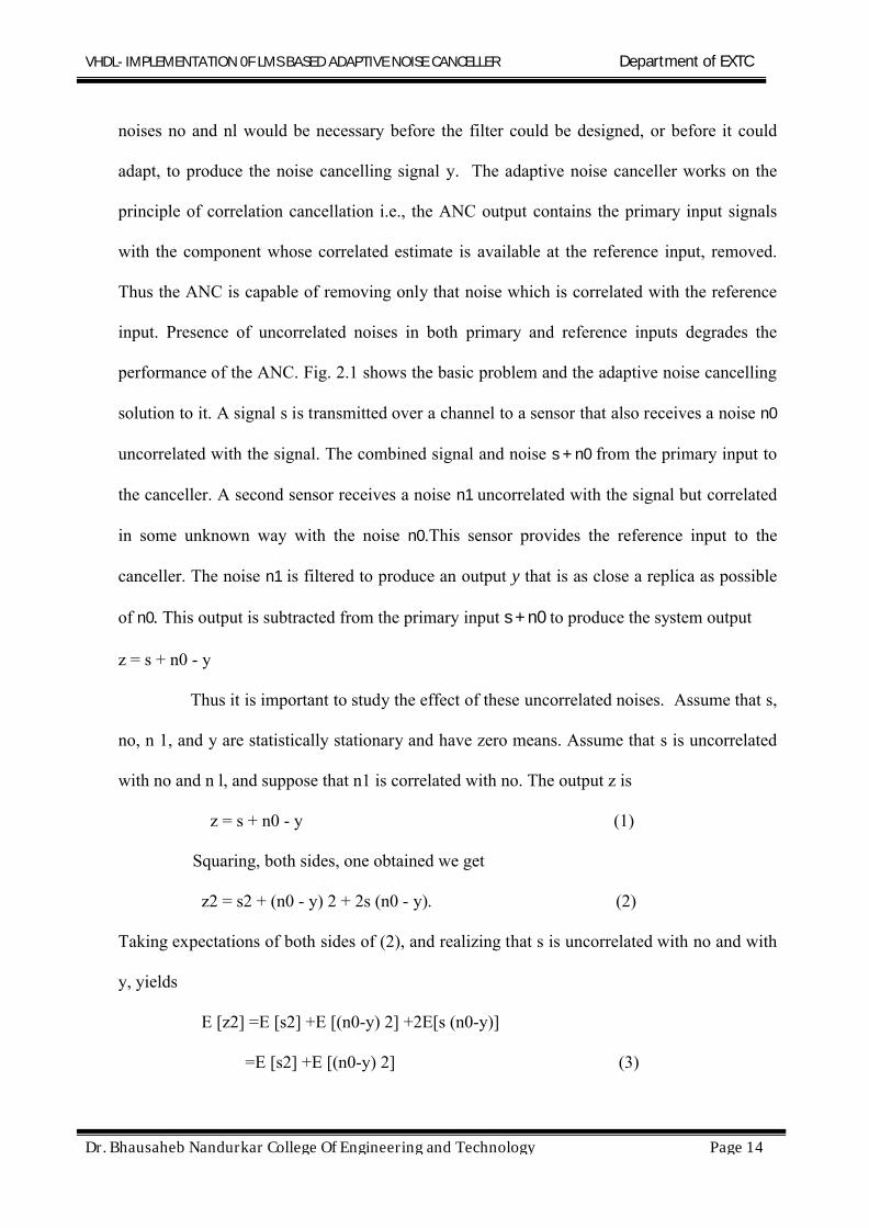
z = s + n0 - y
Thus it is important to study the effect of these uncorrelated noises. Assume that s,
no, n 1, and y are statistically stationary and have zero means. Assume that s is uncorrelated
with no and n l, and suppose that n1 is correlated with no. The output z is
z = s + n0 - y (1)
Squaring, both sides, one obtained we get
z2 = s2 + (n0 - y) 2 + 2s (n0 - y). (2)
Taking expectations of both sides of (2), and realizing that s is uncorrelated with no and with
y, yields
E [z2] =E [s2] +E [(n0-y) 2] +2E[s (n0-y)]
=E [s2] +E [(n0-y) 2] (3)
VHDL- IMPLEMENTATION 0F LMS BASED ADAPTIVE NOISE CANCELLER Department of EXTC
Dr. Bhausaheb Nandurkar College Of Engineering and Technology Page 15
The signal power E [s 2] will be unaffected as the filter is adjusted to minimize E [z2].
Accordingly, the minimum output power is
Min e [z2] =E [s2] +min e [(n0-y) 2] (4)
When the filter is adjusted so that E [z2] is minimized, E [(n0 -y) 2] is also
minimized. The filter output y is then a best least squares estimate of the primary noise n0.
Moreover, when E [(n0 - y) 2] is minimized [(z -s) 2] is also minimized, since, from (I),
(z - s) = (n0 - y). (5)
Adjusting the filter to minimize the total output power is thus to causing the output z to be a
best least squares estimate of the s for the given structure and adjustability of the adaptive
filter and for the given reference input. The output z will contain the signal s plus noise. From
equation (l), the output noise is given by (n0 -y). Since minimizing E [z2] minimizes E [(n0 -
y) 2] minimizing the total output power minimizes the output noise power. Since the signal in
the output remains constant, minimizing the total output power maximizes the output signal-
to-noise ratio.
4.2 LMS adaptive algorithm
The Least Mean Square (LMS) algorithm, introduced by Widrow and Hoff in
1959 is an adaptive algorithm, which uses a gradient-based method of steepest decent. LMS
algorithm uses the estimates of the gradient vector from the available data. LMS incorporates
an iterative procedure that makes successive corrections to the weight vector in the direction
of the negative of the gradient vector which eventually leads to the minimum mean square
error. Compared to other algorithms LMS algorithm is relatively simple; it does not require
correlation function calculation nor does it require matrix inversions. The optimum tap-
weights of a transversal (FIR) Wiener filter can be obtained by solving the Wiener-Hoff
equation provided that the required statistics of the underlying signals are available.
VHDL- IMPLEMENTATION 0F LMS BASED ADAPTIVE NOISE CANCELLER Department of EXTC
Dr. Bhausaheb Nandurkar College Of Engineering and Technology Page 16
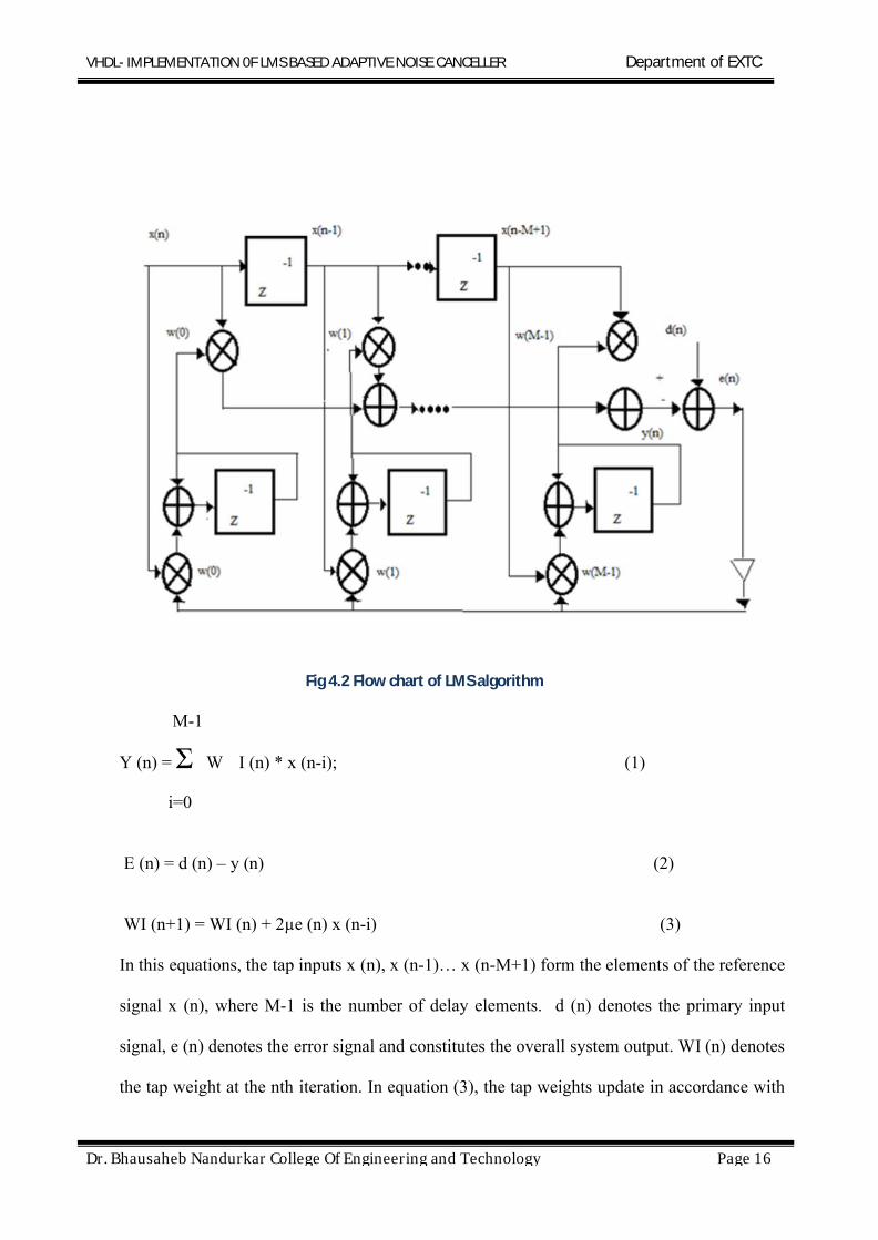
Fig 4.2 Flow chart of LMS algorithm
M-1
Y (n) = Σ W I (n) * x (n-i); (1)
i=0
E (n) = d (n) – y (n) (2)
WI (n+1) = WI (n) + 2µe (n) x (n-i) (3)
In this equations, the tap inputs x (n), x (n-1)… x (n-M+1) form the elements of the reference
signal x (n), where M-1 is the number of delay elements. d (n) denotes the primary input
signal, e (n) denotes the error signal and constitutes the overall system output. WI (n) denotes
the tap weight at the nth iteration. In equation (3), the tap weights update in accordance with
VHDL- IMPLEMENTATION 0F LMS BASED ADAPTIVE NOISE CANCELLER Department of EXTC
Dr. Bhausaheb Nandurkar College Of Engineering and Technology Page 17
the estimation error and scaling factor u is the step-size parameter µ controls the stability and
convergence speed of the LMS. It produces four enable signals: en x, en d, en coeff, en err,
which enable the Delay Block, the Weight Update Block and the Error Counting Block
separately. The Delay Block receives the reference signal x in and the primary input signal d
in under control of the enable signal en x and en d. And it produces the M tap delay signal x
out.
The Error Counting Block subtracts yn from dn and get the error signal e out
which is also the output of the whole system. And it produces signal x as a feedback by
multiplying s out, xout. The Weight Update Block updates the weight vector w (n) to w (n+1)
that will be used in the next iteration. We programmed the delay block with VHDL under the
platform of Xilinx ISE 13.1. In this block we have to apply one reference input containing
noise i.e. x in and one primary input containing the corrupted signal i.e. d in and two enable
signals en x & en d so that we get the delay output x out. When both the enable signals get 0
then we have to produce one delay signal so that our reference input and primary input are
not mixed.

VHDL- IMPLEMENTATION 0F LMS BASED ADAPTIVE NOISE CANCELLER Department of EXTC
Dr. Bhausaheb Nandurkar College Of Engineering and Technology Page 18
CHAPTER 5
FIR FILTER STRUCTURE:-
5.1 Realization of FIR filter
The impulse response h (n) of finite unit impulse response filter with sequence
of length N, the transfer function usually has the following from
(3.1)
Differential equation can be described as
(3.2)
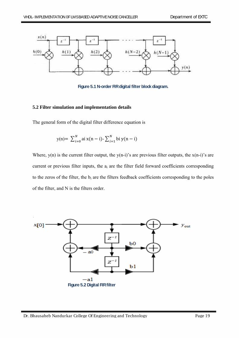
As it can be seen from the differential equation(3.2), FIR filter order is N-I, length is N.
System output depends on a function of the input and has no direct relationship with the past
output, it does not contain feedback branch. y(n) is the output and x(n-i) is the input sample
sequence on the nth times. h(i) is the ith level filter tap coefficient, L is the number of the
filter tap. Its basic structure is shown in Fig. 1. We can find that the structure of FIR filter in
hardware is mainly composed of the shift register, adder and multiplier.
VHDL- IMPLEMENTATION 0F LMS BASED ADAPTIVE NOISE CANCELLER Department of EXTC
Dr. Bhausaheb Nandurkar College Of Engineering and Technology Page 19
Figure 5.1 N-order FIR digital filter block diagram.
5.2 Filter simulation and implementation details
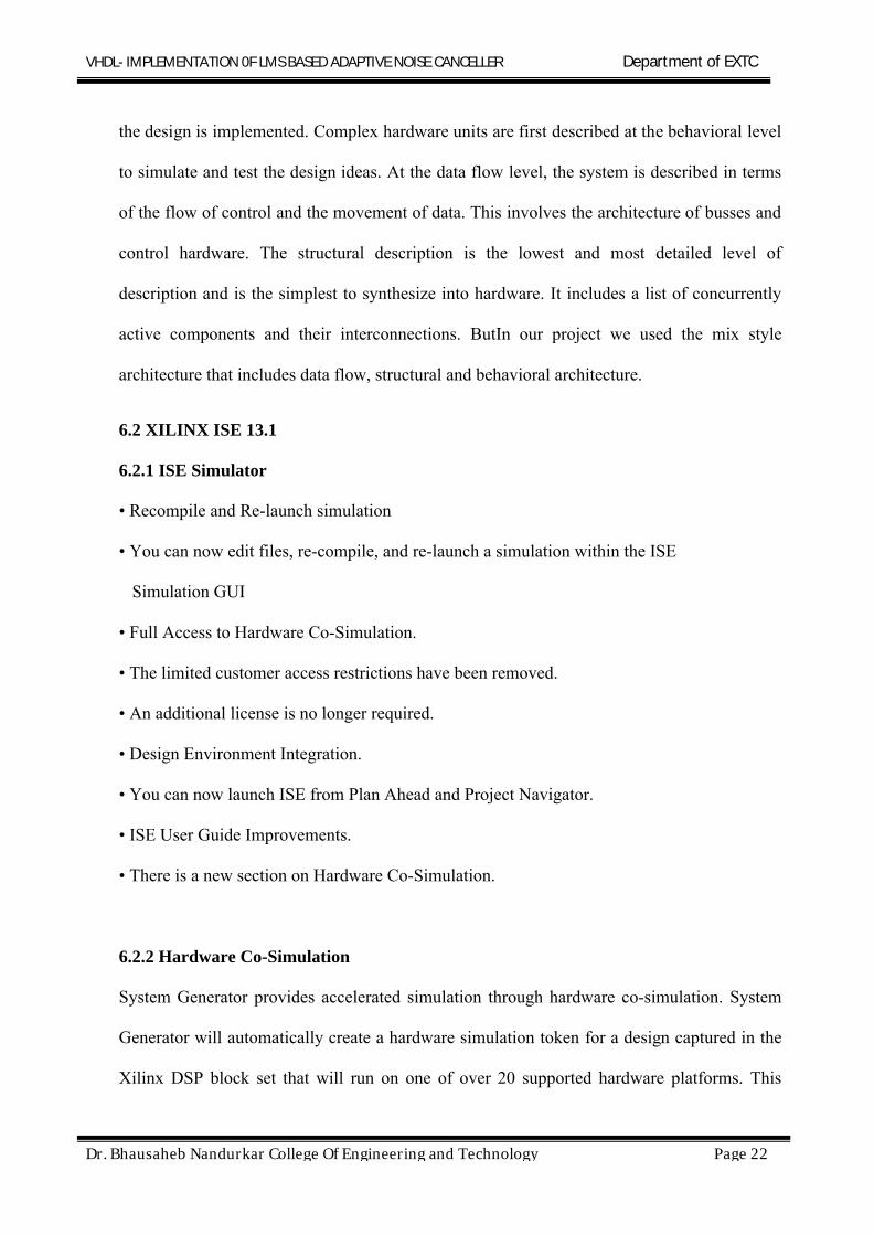
The general form of the digital filter difference equation is
y(n)= ai x(n − i)- bi y(n − i)Where, y(n) is the current filter output, the y(n-i)’s are previous filter outputs, the x(n-i)’s are
current or previous filter inputs, the ai are the filter field forward coefficients corresponding
to the zeros of the filter, the bi are the filters feedback coefficients corresponding to the poles
of the filter, and N is the filters order.
Figure 5.2 Digital FIR filter

VHDL- IMPLEMENTATION 0F LMS BASED ADAPTIVE NOISE CANCELLER Department of EXTC
Dr. Bhausaheb Nandurkar College Of Engineering and Technology Page 20
Very high speed hardware description language (VHDL) has strong abstract description
ability to support hardware design, verification, synthesis and testing. VHDL can describe the
same logic function in multiple levels, such as it can describe the structure of the circuit
composition in the register level and describe the function and performance of the circuit in
the behavior level. VHDL has been used to enter hardware description of FIR filter. The filter
design has been prototyped on an XC3S500-4FG320 FPGA device in Spartan-3E Platform
using ISE 13.1, tools all in one design suit from Xilinx.

VHDL- IMPLEMENTATION 0F LMS BASED ADAPTIVE NOISE CANCELLER Department of EXTC
Dr. Bhausaheb Nandurkar College Of Engineering and Technology Page 21
CHAPTER 6
SOFTWARE PLATFORM USED:-
6.1 General description of VHDL
Hardware description languages (HDLs) are used to describe hardware for the
purpose of simulation, modeling, design, testing and documentation. These languages are
used to represent the functional and wiring details of digital systems in a compact form. It
must uniquely and unambiguously define the hardware at various levels of abstraction. The
IEEE standard VHDL is such a language. VHDL stands for VHSIC HDL where VHSIC
stands for Very High Speed Integrated Circuit. It was developed in 1981 by the US
Department of Defense as a language to describe the structure and function of hardware.
IEEE standardized it in 1987. It is widely used as a standard tool for the design,
manufacturing and documentation of digital circuits at various levels of complexity. The only
other major HDL which is prevalent is the IEEE standard Verilog HDL. VHDL is a general
purpose hardware description language which can be used to describe and simulate the
operation of a wide range of digital systems starting with those containing only a few gates
up to systems formed by the interconnection of many complex integrated circuits.
A VHDL description has two main parts. They are the entity part and the architecture
part. The entity describes the system as a single component as seen by external devices. This
part provides information about the system’s interface while revealing nothing about its
internal structure and behavior. The architecture part of a VHDL description is used to
specify the behavior and the internal structure of the system. The various architecture are
used in VHDL like behavioral, data flow and structural models. At the behavioral model, the
digital system is described by the functions that it performs. It provides no details as to how
VHDL- IMPLEMENTATION 0F LMS BASED ADAPTIVE NOISE CANCELLER Department of EXTC
Dr. Bhausaheb Nandurkar College Of Engineering and Technology Page 22
the design is implemented. Complex hardware units are first described at the behavioral level
to simulate and test the design ideas. At the data flow level, the system is described in terms
of the flow of control and the movement of data. This involves the architecture of busses and
control hardware. The structural description is the lowest and most detailed level of
description and is the simplest to synthesize into hardware. It includes a list of concurrently
active components and their interconnections. ButIn our project we used the mix style
architecture that includes data flow, structural and behavioral architecture.
6.2 XILINX ISE 13.1
6.2.1 ISE Simulator
• Recompile and Re-launch simulation
• You can now edit files, re-compile, and re-launch a simulation within the ISE
Simulation GUI
• Full Access to Hardware Co-Simulation.
• The limited customer access restrictions have been removed.
• An additional license is no longer required.
• Design Environment Integration.
• You can now launch ISE from Plan Ahead and Project Navigator.
• ISE User Guide Improvements.
• There is a new section on Hardware Co-Simulation.
6.2.2 Hardware Co-Simulation
System Generator provides accelerated simulation through hardware co-simulation. System
Generator will automatically create a hardware simulation token for a design captured in the
Xilinx DSP block set that will run on one of over 20 supported hardware platforms. This

VHDL- IMPLEMENTATION 0F LMS BASED ADAPTIVE NOISE CANCELLER Department of EXTC
Dr. Bhausaheb Nandurkar College Of Engineering and Technology Page 23
hardware will co-simulate with the rest of the Simulink system to provide up to a 1000x
simulation performance increase.
Figure 6.1 Hardware co-simulation
6.2.3 System Integration Platform
System Generator provides a system integration platform for the design of DSP FPGAs
that allows the RTL, Simulink, MATLAB and C/C++ components of a DSP system to come
together in a single simulation and implementation environment. System Generator supports
a black box block that allows RTL to be imported into Simulink and co-simulated with either

VHDL- IMPLEMENTATION 0F LMS BASED ADAPTIVE NOISE CANCELLER Department of EXTC
Dr. Bhausaheb Nandurkar College Of Engineering and Technology Page 24
Model Simulation or Xilinx® ISE® Simulator. System Generator also supports the inclusion
of a Micro Blaze® embedded processor running C/C++ programs.
6.3 Spartan-3 FPGA
This section of the manual describes the hardware of the Spartan-3 Development
board. The hardware was designed with the Spartan-3 FPGA as the focal point. The block
diagram is shown in Figure 6.2.
Figure 6.2 Spartan-3 FPGA
The Spartan-3 Development board was designed to support the Spartan-3 FPGA in
the 676-pin, BGA package (FG676). The FG676 package supports three mid-range densities
(1000, 1500, and 2000). The board was designed to support two of the three densities: the
3S1500 and 3S2000. The schematic symbol used for the Spartan-3 device indicates the
specific I/O pins available in each density (396 I/Os with 2VP7 and 556 I/Os with the
2VP20/30). Table 3 describes the attributes of the Spartan-3 device based on density.
VHDL- IMPLEMENTATION 0F LMS BASED ADAPTIVE NOISE CANCELLER Department of EXTC
Dr. Bhausaheb Nandurkar College Of Engineering and Technology Page 25
6.3.1 Configuration
The Spartan-3 Development board supports Boundary-scan as well as Master/Slave
Serial and Master/Slave Parallel (Select MAP) using the on-board PROMs. All configuration
pins are brought out to “J1”, should the user wish to program with an alternate method.
6.3.2 Boundary scan
Programming the Spartan-3 FPGA via Boundary-scan requires a JTAG download cable. The
Spartan-3 Development board has connectors to support both the flying leads connection of
the Parallel Cable III and the ribbon cable connection of the Parallel Cable IV. These
connectors are labeled “J1” and “J5” respectively.
The FPGA and Platform Flash are both in the JTAG chain and both may be
configured via the chain. When programming the FPGA via the JTAG interface, it is good
practice to place the device in Boundary Scan mode. This may be accomplished using the
Mode select jumpers at JP2. The jumper positions are labeled M0 – M2 and are all LOW by
default. So placing a jumper provides a HIGH. The Spartan-3 FPGA is set to Master Serial
mode when no jumpers are installed on JP2. To set the FPGA to boundary-scan mode, install
shunts on JP2 at locations 1-2 & 5-6 as shown in below. Note that power should be removed
when changing Mode select jumpers.

VHDL- IMPLEMENTATION 0F LMS BASED ADAPTIVE NOISE CANCELLER Department of EXTC
Dr. Bhausaheb Nandurkar College Of Engineering and Technology Page 26
CHAPTER 7
WORKING: -
7.1 Working flow chart of adaptive filter
Figure 7 Flow Chart
An adaptive noise canceller works on principle of correlation cancelation. Basically
adaptive canceller having dual input closed loop adaptive feedback system. The main
function of adaptive filter is removing the noise at output signal by adjusting filter
coefficient using LMS algorithm. The working of adaptive canceller explains by flow chart.
VHDL- IMPLEMENTATION 0F LMS BASED ADAPTIVE NOISE CANCELLER Department of EXTC
Dr. Bhausaheb Nandurkar College Of Engineering and Technology Page 27
Mainly in our project we used two 8 bit inputs. One is desired input Din and another
reference correlated noisy input Xin. The desired input signal which is corrupted by noise
that can be obtained by applying main input signal X(k) and noisy input signal N(k) to
adder. This adder adds input signal and noisy signal and gives corrupted signal. It further
supplied to FIR filter as an input signal. The FIR filter has its own impulse response. FIR
filter convolutes input signal with its own impulse response. Then FIR filter give a desired
output signal. This is the first iteration which cannot solve the problem completely. It then
further forward to adaptive LMS algorithm as a input signal. Another reference noisy
correlated input is also given to adaptive LMS algorithm. The Least Mean Square (LMS) is
a simple well behaved algorithm which is commonly used in applications where a system
has to adapt to its environment. LMS algorithm continuously compares input signal with
reference signal for adjusting the filter coefficients. After every iteration, the filter
coefficients get updated. It’s output is further applied to FIR filter again which will again
performs filtering to give error output signal. After the certain number of iterations, we will
get the required noise free output. The adaptive filter differs from a fixed filter in that it
automatically adjusts its own impulse response. Adjustment is accomplished through an
algorithm that responds to an error signal.

VHDL- IMPLEMENTATION 0F LMS BASED ADAPTIVE NOISE CANCELLER Department of EXTC
Dr. Bhausaheb Nandurkar College Of Engineering and Technology Page 28
CHAPTER 8
APPLICATIONS:-
8.1 Application of adaptive filter on ECG
Adaptive filters have become much more common and are now routinely used
in devices such as mobile phones and other communication devices, camcorders and digital
cameras, and medical monitoring equipment.
Suppose a hospital is recording a heart beat (an ECG) which is being corrupted
by a 50 Hz noise (the frequency coming from the power supply in many countries). However,
due to slight variations in the power supply to the hospital, the noise signal may
contain harmonics of the noise and the exact frequency of the noise may vary. One way to
remove the noise is to filter the signal with a notch filter at 50 Hz. Such a static filter would
need to remove all the frequencies in the vicinity of 50 Hz, which could excessively degrade
the quality of the ECG since the heart beat would also likely have frequency components in
the rejected range.
To circumvent this potential loss of information, an adaptive filter could be used. The
adaptive filter would take input both from the patient and from the power supply directly and
would thus be able to track the actual frequency of the noise as it fluctuates. Such an adaptive
technique generally allows for a filter with a smaller rejection range which means in our case
that quality of the output signal is more accurate for medical diagnoses.
VHDL- IMPLEMENTATION 0F LMS BASED ADAPTIVE NOISE CANCELLER Department of EXTC
Dr. Bhausaheb Nandurkar College Of Engineering and Technology Page 29
8.2 Application of adaptive noise filter on echo cancellation
In telecommunications, echo can severely affect the quality and intelligibility
of voice conversation in telephone, teleconference or cabin communication systems. The
perceived effect of an echo depends on its amplitude and time delay. In general, echoes with
appreciable amplitudes and a delay of more than 1 ms can be noticeable. Echo cancellation is
an important aspect of the design of modern telecommunications systems such as
conventional wire-line telephones, hands-free phones, cellular mobile (wireless) phones,
teleconference systems and in-car cabin communication systems. In transmission networks
the echoes are generated when a delayed and attenuated version of the signal sent by the local
emitter to the distant receiver reaches the local receiver. These echo signals have their origin
in the hybrid transformers which perform the two/four-wire conversion, in the impedance
mismatches along the two-wire lines, and in some cases in acoustic couplings between
loudspeakers and microphones in the subscriber sets. The echo cancellation consists in
modeling these unwanted couplings between local emitters and receivers and subtracting a
synthetic echo from the real echo. According to the nature of the signals involved, the system
will work as echo data canceller or voice echo canceller.
8.2.1 Voice echo canceller
Due to the characteristics of the speech signal, the voice echo cancellation
system is somewhat different from the data echo canceller. The speech is a high level non-
stationary signal and due to the signal bandwidth and the velocity of the acoustic waves in the
open air, the filters must have a very long number of coefficients. Also in order to reach a
high level of performance and meet the expectations of the user, the voice echo canceller may
have several other functions, like speech detection and de-noising. The speech signal on the
line from speaker A to speaker B is input to the four/two-wire hybrid B and to the echo

VHDL- IMPLEMENTATION 0F LMS BASED ADAPTIVE NOISE CANCELLER Department of EXTC
Dr. Bhausaheb Nandurkar College Of Engineering and Technology Page 30
canceller. The echo canceller monitors the signal on line from B to A and attempts to model.
The echo path and synthesis a replica of the echo of speaker A. This replica is used to
subtract and cancel out the echo of speaker A on the line from B to A. The echo canceller is
basically an adaptive filter. The co-coefficients of the filter are adapted so that the energy of
the signal on the line is minimized.
8.2.2 Multiple-input multiple-output (MIMO) echo cancellation
Multiple-input multiple-output (MIMO) echo-cancellation systems have
applications in car cabin communications systems, stereophonic teleconferencing systems
and conference halls. Stereophonic echo cancellation systems have been developed relatively
recently and MIMO systems are still the subject of ongoing research and development. In a
typical MIMO system there are P speakers and Q microphones in the room. As there is an
acoustic feedback path set up between each speaker and each microphone, there are
altogether P ×Q such acoustic feedback paths that need to be modeled and estimated. The
truncated impulse response of each acoustic path from loudspeaker i to microphone j is
modeled by an adaptive canceller.
8.3 Application of adaptive noise cancelling filter on ac electrical measurements
Through adaptive noise cancellation it could be improved the ac electrical
measurements. Often ac measurement circuits are influenced by noise caused by line
frequency beat. The figure 16 shows a system that cancels the line frequency beat. An ADC
is used to sample the suitably divided down line voltage in order to determine the phase
relative to the signal channel, which is sampled with a second ADC.
The phase data is used as the noise input to an adaptive noise-cancelling filter
used to cancel the effect on the trans-conductance amplifier output data. Another common
VHDL- IMPLEMENTATION 0F LMS BASED ADAPTIVE NOISE CANCELLER Department of EXTC
Dr. Bhausaheb Nandurkar College Of Engineering and Technology Page 31
interference in ac measurement circuits is the coupling of the magnetic field generated by a
nearby source. In such situations it may be possible to use an adaptive interference cancelling
system with a simple coil system to measure the ambient magnetic field that causes the
unwanted interference and then remove this interference from data obtained from a
measurement circuit.
8.4 Application of adaptive filter on multipath fading
Fading often poses a serious hindrance in radio communication. This multipath
fading problem reduces by the application of a least-mean square (LMS) adaptive filter..
However, it is known that multipath components are in general correlated with one another.
We examine the effect or the correlation on the performance of the LMS adaptive filter. The
LMS adaptive filter suppresses the multipath signal. On the other hand, when the correlation
coefficient nearly equals to the LMS adaptive filter prevents the output signal power from
decreasing. Therefore, the LMS adaptive filter may reduce the multipath fading effectively
for any correlation coefficient value. A reference signal in the LMS adaptive filter is also
discussed. It is shown that synchronization in the reference signal generation must be
extremely accurate. Moreover, a processor configuration is proposed which may generate the
reference signal with the required accuracy.

VHDL- IMPLEMENTATION 0F LMS BASED ADAPTIVE NOISE CANCELLER Department of EXTC
Dr. Bhausaheb Nandurkar College Of Engineering and Technology Page 32
CHAPTER 9
ADVANTAGES:-
Using FPGAs to design adaptive cancellers has several advantages.
1) There are advantages, which have been discussed above, that are
associated with digital filters compared to analog filters.
2) The cost of the FPGA is low and allows the addition of blocks for processing.
3) The design can be easily modified.
4) The adaptive canceller’s frequency response in the interest band is flatter than the analog
notch filter.
5) The bandwidth of the attenuated band of the adaptive canceller is much smaller than that of
the analog notch filter.
6) With specifically oriented architecture, a faster processing speed can be obtained and thus, it
can process signals with a broad bandwidth.
7) Concurrent programming algorithms allow parallel signal processing using only one FPGA
with several input ECG signals without a loss of speed in the process.
8) The adaptive canceller has been tested with signals that simulate the ECG of a patient and the
power-line interference. The results show the correct operation of the adaptive canceller in
this kind of applications.

VHDL- IMPLEMENTATION 0F LMS BASED ADAPTIVE NOISE CANCELLER Department of EXTC
Dr. Bhausaheb Nandurkar College Of Engineering and Technology Page 33
CHAPTER 10
FUTURE SCOPE:-
1) Biomedical signal analysis.
2) Audio processing.
3) Video processing.
4) Medical equipment
5) AC electrical instruments.

VHDL- IMPLEMENTATION 0F LMS BASED ADAPTIVE NOISE CANCELLER Department of EXTC
Dr. Bhausaheb Nandurkar College Of Engineering and Technology Page 34
CHAPTER 11
SIMULATION AND RESULT:-
An adaptive filter module is designed using VHDL. The inputs to this module are :
1. Input signal( Xin) 8 bits
2. Desired signal (Din)8 bits
3. Clock input(clk)
The output are;
1. Error output ( eout) 16 bits
2. Final output (Yout) 16 bits
3. Frequency output.
(F0out 8 bits, F1out 8 bits)
11.1 Entity of Adaptive noise canceller
Figure 11.1 Entity of adaptive noise canceller

VHDL- IMPLEMENTATION 0F LMS BASED ADAPTIVE NOISE CANCELLER Department of EXTC
Dr. Bhausaheb Nandurkar College Of Engineering and Technology Page 35
9.2 Actual gate implementation of adaptive noise canceller
Figure 11.2 Actual gate implementation of adaptive noise canceller

VHDL- IMPLEMENTATION 0F LMS BASED ADAPTIVE NOISE CANCELLER Department of EXTC
Dr. Bhausaheb Nandurkar College Of Engineering and Technology Page 36
11.3 Simulation Result
The code is written in a hardware description language called VHDL and it is simulated in
xillinx 13.1.
Figure 11.3 Simulation

VHDL- IMPLEMENTATION 0F LMS BASED ADAPTIVE NOISE CANCELLER Department of EXTC
Dr. Bhausaheb Nandurkar College Of Engineering and Technology Page 37
CHAPTER 12
CONCLUSION
VHDL implementation of LMS based adaptive noise canceller using parallel
architecture is done successfully. Biomedical signal and multipath fading are supplied as a
primary input to adaptive noise canceller. LMS incorporates an iterative procedure that
makes successive corrections to the weight vector in the direction of the negative of the
gradient vector which eventually leads to the minimum mean square error.
VHDL- IMPLEMENTATION 0F LMS BASED ADAPTIVE NOISE CANCELLER Department of EXTC
Dr. Bhausaheb Nandurkar College Of Engineering and Technology Page 38
CHAPTER 13
REFERENCES
1. R. Ramos, A. Manual, G. Olivar, E. Trullols and J. Del Rio for Application by
means of an adaptive canceller 50 Hz interference in ECG.”May 21-23, 2001.
2. Jones D. L “FIR filter structure version 1.2” Oct 10, 2004.
3. Rafael Ramos Antoni Manuel- Lazaro, Joaquin Del Rio, and Gerard Olivar, Member
IEEE for “FPGA-Based Implementation of an Adaptive Canceller for50/60-Hz Interference
in ECG” DEC 2007.
4. Zhiguo Zhou, Jing He, and Zhiwen Liu for “FPGA-Implementation of LMS
Adaptive Noise Canceller for ECG Signal Using Model Based Design.” 1July, 2011.
5. Mamta M. Mahajan, & S. S. Godbole For “Design Least Mean Square for Adaptive Noise
Canceller”, 2011, www.ijaest.iserp.org.
6. Abhay R. Kasetwar, Sanjay M. Gulhane “A Survey of FPGA Based Interference
Cancellation Architectures for Biomedical Signals” Jan 4-6, 2013.
7. ISE Design Suite 13: Release Notes Guide UG631 (v 13.1), www.xilinx.com.
8. Bhaskar J., “ VHDL primer 3rd Edition Pearson education Asia publication”
9. B. Widrow., “Adaptive noise cancelling: Principles and applications,” Proceedings
of IEEE.


