

Resource Management with Smart Antenna in CDMA Systems
by
Yu Lei
Thesis submitted to the Faculty of the Virginia Polytechnic Institute & State University
in partial fulfillment of the requirements for the degree of
MASTER OF SCIENCE in
Electrical Engineering
Approved:
Dr. Annamalai Annamalai, Chairman
Dr. Lamine Mili Dr. Luiz DaSilva
September 15, 2001 Alexandria, Virginia
Keywords: Smart Antenna, Resource Management, Wideband CDMA, Wireless Communications, Simulation
Copyright 2001, Yu Lei

Resource Management with Smart Antenna in CDMA Systems
Yu Lei
(ABSTRACT)
Third generation (3G) mobile communication systems will provide services
supporting high-speed data network and multimedia applications in addition to voice
applications. The Smart antenna technique is one of the leading technologies that helps to
meet the requirement by such services to radio network capacity. Resource management
schemes such as power control, handoff and channel reservation/assignment are also
essential for providing the seamless services with high quality. Smart antenna techniques
will help to enhance the capability of resource management through more efficient and
flexible use of resources. In this thesis, adaptive array and switched beam antenna
techniques are compared in terms of algorithm, performance, complexity and hardware
requirements. Based on these comparisons, sub-optimal code gate algorithm are most
likely the suitable algorithms for next generation code division multiple access (CDMA)
systems due to its good performances, robustness, and low complexity. A multi-cell
CDMA simulator is developed for investigating the gain from smart antenna techniques
in both bit error rate (BER) performance improvement and enhancement to resource
management schemes. Our study shows that smart antenna techniques can significantly
improve the performance of the system and help to build more powerful and flexible
resource management schemes. With eight array elements, the system capacity can be
increased by a factor of four. Power control command rates can be reduced through the
tradeoff with the interference reduction by smart antennas. Smart antennas will also
reduce handover failure rates and further increase the system capacity by reducing the
resources reserved for soft handover.

iii
Acknowledgments
I would like to express my gratitude to Dr. Annamalai Annamalai for his precious
guidance, support and encouragement during the last one year, essential to my thesis
work. I also thank Dr. Luiz DaSilva and Dr. Lamine Mili for their careful review of my
thesis and valuable suggestions. I also want to express my thankfulness to LG Electronics
for sponsoring the project on which this thesis is based.
Special thanks to Fakhrul Alam and Paulo Cardieri whose works on simulating W-
CDMA systems and resource management gave me introductory knowledge in
constructing my simulation model. I would also like to thank James Hicks and Kazi
Zahid who gave me insight on smart antenna techniques. Shakheela H. Marikar, and
Vikash Srivastava deserve my thankfulness for their help in building the simulation
model.
I would give my thanks to all the faculty members and friends who helped me in
Blacksburg as well as Alexandria during my course and research works for the last two
years.
Finally, I want to thank my parents and family for their unreserved love and support
from where comes the motivation and inspiration for the completion of my thesis work.

iv
List of Content
1. Introduction ...................................................................................................................... 1
1.1 Evolution of Cellular Systems................................................................................... 1
1.2 WCDMA Features..................................................................................................... 3
1.3 Overview of Smart Antenna Techniques................................................................... 5
1.4 Overview of Radio Resource Management............................................................... 6
1.5 Objective and Outline of the Thesis .......................................................................... 8
2. Smart Antenna Techniques ............................................................................................ 10
2.1 Antenna Array Basics.............................................................................................. 10
2.1.1 Uniformly Spaced Isotopic Liner Array Synthesis ........................................... 11
2.1.2 Beamforming..................................................................................................... 12
2.1.3 Sidelobe Reduction ........................................................................................... 14
2.2 Switched Beam Systems.......................................................................................... 15
2.3 Adaptive Beamforming ........................................................................................... 19
2.3.1 Algorithm Basics............................................................................................... 19
2.3.2 Blind Algorithms............................................................................................... 22
2.3.3 Blind Algorithms in CDMA Systems ............................................................... 24
2.4 Complexities and Hardware Requirements of CDMA SA Algorithms .................. 27
2.5 Application Issues of SA in CDMA systems .......................................................... 29
2.5.1 Performance and Beam Pattern ......................................................................... 29
2.5.2 AOA Spread and 2-D RAKE ............................................................................ 32
2.5.3 SA Applications in CDMA Systems................................................................. 35
3. Radio Resource Management......................................................................................... 36
3.1 Introduction to Resource Management.................................................................... 36

v
3.2 Resource management in TDMA/FDMA systems.................................................. 37
3.3 Power Control in CDMA Systems .......................................................................... 40
3.4 Handover in CDMA Systems .................................................................................. 44
3.5 Call Admission Control in CDMA Systems ........................................................... 46
3.6 Capacity Reservation/Channel Assignment in CDMA systems.............................. 47
4. Simulation Model on SA and RRM in CDMA Systems................................................ 51
4.1 General Description of The Simulator..................................................................... 51
4.2 Mobility and Geographic Model ............................................................................. 53
4.3 Event Simulator ....................................................................................................... 60
4.4 Channel Simulator ................................................................................................... 62
4.5 Signal Processor ...................................................................................................... 65
4.6 Smart Antenna Processing....................................................................................... 70
4.7 Resource Management ............................................................................................ 71
5. Simulation Result and Discussions ................................................................................ 73
5.1 General Description of the Simulation Setup .......................................................... 73
5.2 Simulation Study in Single Cell Scenario ............................................................... 74
5.2.1 Single User BER Performance and Power Control........................................... 74
5.2.2 Multi-user BER Performance and Smart Antenna............................................ 80
5.2.3 Cell Capacity, Block/Drop Rate and Smart Antenna ........................................ 84
5.3 Simulation Study in Multi-cell Scenario ................................................................. 87
6. Conclusion and Future Work ......................................................................................... 93
6.1 Conclusions ............................................................................................................. 93
6.2 Future Works ........................................................................................................... 94
Reference .......................................................................................................................... 96
Abbreviations.................................................................................................................. 102
VITA............................................................................................................................... 104

vi
List of Tables Table 1.1 WCDMA, GSM and IS-95 Air Interfaces.......................................................... 3
Table 1.2 Experimental SA Systems and Commercially Available Products.................... 6
Table 1.3 Comparisons of RRM of FDMA/TDMA and CDMA systems ......................... 7
Table 2.1 Criteria for Optimal Weights ........................................................................... 20
Table 2.2 Performance of Switched Beam and Adaptive Array ...................................... 33
Table 4.1 Cluster Sets for Distance Adjustment .............................................................. 60
Table 4.2 Vehicular Outdoor Channel PDF..................................................................... 63
Table 5.1 Number of Users with respect to Arrival/Departure Ratio ............................. 84

vii
List of Figures
Fig 1.1 UTRAN Architecture ............................................................................................. 4
Fig 2.1 Uniformly Spaced Isotopic Linear Array............................................................. 12
Fig 2.2 Beam Pattern of a 8 Element Linear Array .......................................................... 14
Fig 2.3 Comparison of Beam Pattern with Different SLR ............................................... 15
Fig 2.4 Switched Beam System Block Diagram .............................................................. 17
Fig 2.5 Multi-beam Generating Algorithms ..................................................................... 18
Fig 2.6 Multi-beam Patterns of Switched Beam Systems ................................................ 18
Fig 2.7 Reference Generation in Decision Direct Algorithm........................................... 23
Fig 2.8 CGA Beamformer Block Diagram....................................................................... 26
Fig 2.9 CGA and Sub-Optimal CGA Computing process................................................ 28
Fig 2.10 Complexity of the Smart Antenna Algorithms................................................... 28
Fig 3.1 Transmitting Power vs. System Load................................................................... 43
Fig 3.2 IS-95A Handover Process .................................................................................... 44
Fig 3.3 WCDMA Handover Process ................................................................................ 45
Fig 3.4 Channel Reservation Scheme............................................................................... 50
Fig 4.1 General Block Diagram of The Simulator ........................................................... 52
Fig 4.2 PDF of Mobile Directions and Speeds ................................................................. 54
Fig 4.3 Overlapping Area of Cell Styles .......................................................................... 55
Fig 4.4 Coverage Area and Cell Layout ........................................................................... 56
Fig 4.5 Concept of Toroidal Structure.............................................................................. 57
Fig 4.6 Toroidal Adjustment of Mobile Locations and MS to BS Distances.................. 58
Fig 4.7 Mobile Location Adjustment................................................................................ 59
Fig 4.8 Events Generating and Scheduling....................................................................... 61
Fig 4.9 Time Varying Channel ......................................................................................... 65
viii
Fig 4.10 WCDMA Physical Channel Spreading and Modulation.................................... 67
Fig 4.11 Receiver Structure .............................................................................................. 69
Fig 4.12 Smart Antenna Processing.................................................................................. 70
Fig 4.13 CAC and Channel Reservation Scheme............................................................. 72
Fig 5.1 Received Signal at BS .......................................................................................... 75
Fig 5.2 Fading Curves with Different Doppler Spreads ................................................... 76
Fig 5.3 BER with PC under Different Doppler Spread .................................................... 77
Fig 5.4 Power Control Error with Respect to Doppler Spreads ....................................... 78
Fig 5.5 BER with Respect to Doppler Spreads................................................................. 79
Fig 5.6 BER with Respect to Shadowing and Fast/Slow PC............................................ 80
Fig 5.7 BER with respect to PC and Sectoring................................................................. 81
Fig 5.8 BER with respect to SA and Number of Users ................................................... 82
Fig 5.9 BER with respect to SA and No. of Users ........................................................... 83
Fig 5.10 BER with respect to PC Rate and SA................................................................. 84
Fig 5.11 Cell Capacity with respect to Antenna, Call Admission and Drop Threshold... 85
Fig 5.12 Number of Users with Finite Cell Capacity ....................................................... 86
Fig 5.13 Block / Drop Rate and the Antenna.................................................................... 87
Fig 5.14 Call Drop Rate with respect to Antenna Types, SR, and Reservation ............... 88
Fig 5.15 Handover Rate with respect to Antenna Type and SR....................................... 89
Fig 5.16 Handover Failure Rate with respect to Antenna and SR.................................... 90
Fig 5.17 Call Blocking Rates with respect to Antenna Types and SR ............................. 91
Fig 5.18 Call Blocking Rate with respect to Antenna and Reservation ........................... 91
Fig 5.19 Handover Failure Rate with respect to Antenna and Reservation...................... 92

1
Chapter 1
Introduction
1.1 Evolution of Cellular Systems
In the current telecommunication market, mobile phones are predicted to outnumber
the fixed line phones and the mobile phone coverage exceeds 70% in countries with the
most advance wireless markets [1]. So far, cellular technology has been evolving over
two and currently to its third generation. Third generation mobile telecommunication
networks are developed in competing with the traditional wired networks not only in
number of subscribers but also in types of service they provide.
First generation cellular networks are analog systems using Frequency Division
Multiple Access (FDMA). Deployed in 1983 [2], the Advanced Mobile Phone System
(AMPS) is representative of the first generation systems employing FM technology and
cellular concept with frequency reuse and planning.
Second generation systems (2G) dominate the current cellular market. Second
generation cellular systems transmit and process digital signals with sophisticated
signaling, access control and resource management scheme. Global System for Mobile
Communications (GSM) deployed from 1990 [2] is the largest network in Europe and
employs Time Division Multiple Access (TDMA). In the United States, major 2G
standards include IS-95 (cdmaOne) adopted in 1993 [3] based on Code Division Multiple
Access (CDMA) and IS-54/IS-136 based on TDMA. Second generation systems provide
2
a wide range of services such as voice, paging, facsimile, and low speed data network
services.
Third generation systems (3G) have been developed from 2G systems to provide
seamless and integrated voice and data services such as multi-media transmission and
high-speed Internet access with a uniform infrastructure. Basic characteristics of 3G
systems include [4]:
• A common global frequency band for both terrestrial and satellite components
• A small pocket terminal with worldwide roaming
• Maximizing the commonality and optimization of radio interfaces for multiple
environments
• High speed circuit- and packet-switched data transmission and multi-media
service
• Support for both symmetric and asymmetric data capabilities in all environments
• Compatibility with pre-existing networks and new services
• Spectrum efficiency and overall cost improvement
Major proposals for 3G systems based on CDMA techniques include cdma2000,
WCDMA (UTRA, ARIB), CDMA I / CDMA II, and TD-SCDMA. Although most of the
standard proposals avoid adopting specific requirements that result in new receiver
structures, new technologies are available and may be implemented in 3G systems.
Technologies for 3G and 4G systems include smart antenna techniques, multi-user
detection, new receivers structure (such as LMMSE receivers), space-time receiver, turbo
coding, and software radio, etc. [5].

3
1.2 WCDMA Features
WCDMA (UTRA) evolves from GSM system and combines Wideband Direct
Sequence CDMA (DS-CDMA) air interface with GSM radio network structure. Major
characteristics of W-CDMA systems are tabulated below with comparison to GSM and
IS-95 systems [1].
Table 1.1 WCDMA, GSM and IS-95 Air Interfaces
CHARACTORISTICS WCDMA GSM IS-95
Carrier Spacing 5 MHz 200 kHz 1.25 MHz
Chip Rate 3.84 Mcps N/A 1.2288 Mcps
Frequency Reuse Factor 1 1-18 1
BS Synchronization Not needed N/A Typically via GPS
Inter-frequency Handover Yes N/A Possible
Power Control Frequency 1500 Hz 2 Hz or Lower 800Hz
Resource Management Efficient radio
resource management
algorithms
Frequency planning
Not needed for
speech only
networks
Frequency Diversity Rake receiver Frequency hoping Rake receiver
Packet Data Load-based scheduling Time-slot based
scheduling with GPRS
As short circuit
switched calls
Downlink Trans Diversity Supported Not supported but
applicable Not supported
Other characteristics of WCDMA are:

4
• Support for both Frequency Division Duplex (FDD) and Time Division Duplex
(TDD)
• Frame length is 10 ms
• Multi-user detection and smart antennas supported but optional in implementation
• Data rate of 384 kbps for outdoor to indoor and pedestrian, 2 Mbps for indoor
office
• Support for variable rate data service
Fig 1.1 UTRAN Architecture
Figure 1.1 shows the overall structure of the third generation mobile network based
on W-CDMA air interface [1], [44]. The Public Land Mobile Networks (PLMN) consists
of a core network, multiple radio network subsystems (RNS), also called the Universal
Terrestrial Radio Access Networks (UTRAN), and User Equipment (UE). UTRAN
consists of one Radio Network Controller (RNC) and multiple Node BS (Base Station)
Core Network
RNC
Node BS
RNS
Node BS
lub lub
RNC
Node BS
RNS
Node BS
lub lub
lu lu
External Networks (PLMN, PSTN, ISDN, etc.)
UE UE
Uu Uu
UTRAN UTRAN
P L M N

5
under control. Among several interfaces in the system, Uu is the WCDMA air interface
and lub is the interface between a BS and its RNC.
Radio links will be established between Node BS and UE. Smart antenna is set up at
Node BS. Power control will involve both Node BS and UE. Handover, call admission
control (CAC) and channel assignment will in addition involve the RNC.
1.3 Overview of Smart Antenna Techniques
Smart Antenna (SA) techniques employ Digital Beam Forming (DBF) originated in
the sonar and radar communities. Instead of generating an omni-directional beam pattern,
a smart antenna can point one beam to a particular direction from which the desired user
signal comes and nulls the interfering signals from other users. Additional gains also
come from the spatial and angular diversity provided by an antenna array. The carrier to
noise ratio also increases when signals from array elements combine, which yields
multiplied received signal power at the output of the combiner.
Two smart antenna techniques have been developed and implemented in cellular
systems. Switched beam systems use multiple beams of fixed number and directions
while adaptive arrays steer one beam to one individual user. Table 1.2 shows the
experimental and commercially available smart antenna systems [7].
In addition to switched beam and adaptive array, overloaded arrays combine the
techniques of adaptive array and multi-user detection to serve users who outnumber the
array elements by several times. Overloaded array algorithms have been considered
mainly in airborne systems due to its increased complexity as compared to the other two.

6
Table 1.2 Experimental SA Systems and Commercially Available Products
Designer Air Interface
Antenna (M) SA Receiver Algorithm Remarks Ref
SA Experimental Systems
Ericsson & Manesmann Mobilefunk
GSM/DCS 1800 8 Up-link: DOB Down-link: DOB switched beam and adaptive
Several BS with SA in network [8]
Ericsson Research (SW/US)
IS-136 (D-AMPS)
Spacing up-link 15λ & pol. div.
Up-link: MRC and IRC, Down-link: fixed beam approach [9]
AT&T Labs-Research (US) IS-136 4
Up-link: adaptive TRB, DMI Algorithm Down-link: switched beam with or without PC
Up and down links are independent [10]
NTT DoCoMo (Japan) UMTS 6
Up-link: Decision directed MMSE (tentative data and pilot) 4-finger 2D Rake Down-link: Calibration of weights for reverse link
Include 3 cell sites data transmission up to 2 Mbps
[11]
TSUNAMI Consortium (EU)
DECT -> DCS 1800
ULA with MUSIC for AoA estimation, tracking with Kalman filtering
SDMA was studied based on DECT [12]
CNET & CSF-THOMPSON (F) GSM/DCS 1800 10 circular
Up-link: DOB based BF Capon, MUSIC for AoA estimation Down-link: DOB
[13]
Uppsala University (SW) DCS 1800 10 circular Up-link only: TRB with DMI Data traffic from
DCS-1800 used [14]
Commercially Available Products
Metawave (US) SpotlightTM 2000 AMPS, CDMA 12 Up-and down link: 12 switched
beam [15]
Raytheon (US) Flexible upgraded by SW 8 Up-link: DOB
SA can be directly connected at RF input at BS
[16]
ArrayComm IntelliCellTM (US)
WLL, PHS, GSM 4 Up-link: ESPRIT algorithm
Adaptive interference cancellation First mass market commercial product [17]
1.4 Overview of Radio Resource Management
Radio Resource Management (RRM) is essential for efficient utilization of available
air interface and transmitting power, maximizing the system capacity, and guaranteeing
Quality of Service (QoS). Resource management includes functions such as power
7
control (PC), handover, channel assignment, load control and packet scheduling. Such
resource management mechanisms may also interact with each other and desire joint
consideration.
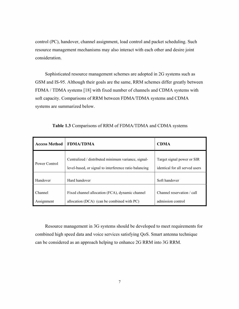
Sophisticated resource management schemes are adopted in 2G systems such as
GSM and IS-95. Although their goals are the same, RRM schemes differ greatly between
FDMA / TDMA systems [18] with fixed number of channels and CDMA systems with
soft capacity. Comparisons of RRM between FDMA/TDMA systems and CDMA
systems are summarized below.
Table 1.3 Comparisons of RRM of FDMA/TDMA and CDMA systems
Access Method FDMA/TDMA CDMA
Power Control Centralized / distributed minimum variance, signal-
level-based, or signal to interference ratio balancing
Target signal power or SIR
identical for all served users
Handover Hard handover Soft handover
Channel
Assignment
Fixed channel allocation (FCA), dynamic channel
allocation (DCA) (can be combined with PC)
Channel reservation / call
admission control
Resource management in 3G systems should be developed to meet requirements for
combined high speed data and voice services satisfying QoS. Smart antenna technique
can be considered as an approach helping to enhance 2G RRM into 3G RRM.

8
1.5 Objective and Outline of the Thesis
The objective of our research is to compare different smart antenna techniques
(switched beam and adaptive array) in aspects including performance, complexity, and
hardware requirements, and to investigate the performance improvement, capacity
increment and resource management (power control, hand off, and channel assignment /
reservation) enhancements brought about by SAs.
Many smart antenna algorithms can be found in literature [6], [19], [22], [23], [24],
[25]. [21] also compared switched beam algorithms with a tracking beam algorithm
(maximum power Lagrange). This thesis studies comprehensively on comparisons among
different smart antenna algorithms subjected to various applications and environments.
Detail comparisons are made to switched beam and adaptive array algorithms applied in
CDMA systems.
Radio resource management (RRM) has been studies by many researchers, e.g.
[33]-[38], [42]. However, there are little discusses on smart antennas effects on radio
resource management in CDMA systems. This thesis studies how smart antenna affect
radio resource management schemes such as power control, handover and radio resource
management.
This research also provides a multi-cell cellular system simulator based on
WCDMA and IS-95 standards that includes smart antenna and resource management
schemes. [18] discussed a simulation model of multi-cell cellular systems in TDMA
systems. There are also works on simulating WCDMA transmitting and receiving
structures [45] in single cell scenario. Different to these works, we developed a CDMA
system simulator in a multi-cell scenario. A new method is presented to generate an
accurate geographic model with toroidal structures essential for studying RRM. Smart
antenna algorithms and radio resource management schemes are also simulated. These

9
simulation are process in WCDMA signals and with mobile movements instead of by
theoretical models.
This thesis is organized as follows. Chapter two introduces beamforming basics and
various smart antenna algorithms. Also discussed are applications of SA in cellular
systems and the comparison between switched beam systems and adaptive array systems.
Chapter three discusses resource management schemes, especially in WCDMA and IS-95
systems. Chapter four describes the simulator for homogeneous or heterogeneous multi-
cell WCDMA cellular systems. Simulation results and observations from the results are
summarized in Chapter five.
10
Chapter 2
Smart Antenna Techniques
Smart antenna began to draw intensive attention from the cellular community in the
early 1990s despite the long history of antenna array applications in radar and sonar
systems. Smart antenna techniques improve point-to-point communications by providing
spatial processing capability. SA techniques not only increase the capacity of the systems
but also provide additional degrees of freedom for the radio network control and
planning.
SA techniques can be integrated into existing and future cellular networks without
major obstacles because of its relative independence to other components of cellular
systems. A large number of algorithms have been developed to meet the need of different
applications and environments. SA can easily be combined with other techniques such as
space-time processing, multi-user detection, and channel coding [7]. SA techniques can
also easily be integrated with radio resource management schemes and provide additional
enhancement and flexibility to the schemes.
2.1 Antenna Array Basics
An antenna array is a set of antenna elements that are spatially distributed at fixed
locations. A beamformer electronically forms the main beam and/or places nulls in any
direction by changing the phase and amplitude of the exciting currents in each of the
antenna elements. Linear, circular and planar arrays are common geometric arrangements
of antenna elements. Linear arrays have their elements aligned along a straight line, and

11
are further called uniformly spaced linear array if the spacing between the array elements
is equal. Circular arrays have their elements placed on a circle. Both linear arrays and
circular arrays belong to the set termed planar array, with all their elements lying on a
plane. Arrays whose elements do not lie on a single plane but conform to a given non-
planar surface are categorized into conformal arrays.
The radiation pattern of an array is determined by the radiation pattern of the
individual elements, their orientations and relative positions in space, as well as the
amplitudes and phases of the feeding currents. If each element of the array is an isotropic
point source, the radiation pattern of the array will depend solely on the geometry and
feeding current of the array [5].
2.1.1 Uniformly Spaced Isotopic Liner Array Synthesis As illustrated in figure 2.1, a uniformly spaced isotopic linear array has equal
distance d between elements and θ as the angle of arrival (AoA) (from broadside to
incident direction). Thus wave front delay between each two adjacent elements is dsinθ
assuming that the array is illuminated by a plane wave. The received signal can be
expressed as:
)()()( 1 txt θαx = (2.1)
where
=
)(
)()(
)( 2
1
tx
txtx
t
M
Mx
=
−−
−
θλπ
θλπ
θ
sin)1(2
sin21
)(
dMj
dj
e
eM
α

12
Fig 2.1 Uniformly Spaced Isotopic Linear Array
2.1.2 Beamforming
Beamforming is a process that generates a radiation pattern from the output of array
elements such that the energy either focuses or disseminates along a specific direction in
space. Electronically scanning of the antenna array can be done using a power dividing
beamforming matrix such as the Butler matrix [19], phase array approaches or optimal
combining.
It is desirable for its simplicity and flexibility to electronically scan the beam of an
antenna by changing the phase of the output from the antenna elements. If only the
phases are shifted with the amplitude unchanged when a beam is steered, the array is
called a phased array [6]. The combined signal after beamforming thus becomes:
)()( tty Hxw= (2.2) where
d1 2 i M
θ
dsinθ
Reference Element
Illuminating
Plane Wave
Wave Plane Front
...

13
=
Mw
ww
M2
1
W
is the weight vector and H denotes the Hermitian transpose. The array response can be
expressed as
)()( θθ αw Hg = (2.3)
Assuming that the weights are all ones, we have
θ
λπ
θλπ
θλ
π
θλ
π
θ
sin)1(
1
sin)1(2
)sinsin(
)sinsin(
)(
dMj
M
i
dij
ed
Md
eg
−−
=
−−
=
=∑ (2.4)
The discriminating capability of a beamformer depends on the ratio of the spatial
aperture of the array to the wavelength. The null-to-null beam width is
)arcsin(2MdBWλθ = (2.5)
Large spacing 2/λ>d will cause spatial alias and create additional main lobes,
while excessively small spacing would bring mutual coupling effect and enlarge beam
width. Thus, it is desired to keep 2/λ=d and accordingly beam width will only be
determined by the number of array elements.
It is also noticeable that near the endfire area, the beam width will grow because
)sin(θd , when AoA deviates from the center of the beam, increases more slowly at the
endfire zone than at the broadside. Also noticeable is that for a linear array, array

14
response is symmetric across the two sides of the array since illuminations from both
sides are identical. As for steering, if the weights vector w is chosen as equal to the
natural array response α , the amplitude of the array response after beamforming will
reach its maximum at the AoA θ.
2.1.3 Sidelobe Reduction The array response pattern (space factor) of an 8-element array is shown in Figure
2.2. The sidelobe ratio (SLR) is about 13 dB. SLR will level at 13.26 dB when the
number of array elements increases. It is desirable to do sidelobe reduction to further
reduce the possible interference coming from the sidelobe direction if SLR is of major
concern.
Fig 2.2 Beam Pattern of a 8 Element Linear Array
A half-wave spaced array yields maximum directivity for a given sidelobe ratio
when all sidelobes are of equal height. Chebyshev polynomials are ideally suited for this
purpose [20]. The Dolph-Chebyshev array algorithm is represented by the following
equations.

15
[ ] NSLRSLR
NhSLRx
12
0
121
1arccoscosh
−+=
−=
(2.6)
∑
−−−= −
mNn N
mNnjNmxT
Nw ππ )12(exp)cos(1
01 (2.7)
The beam pattern illustrated in Figure 2.3 shows that for a fixed number of array
elements, there is a tradeoff between sidelobe reduction (SLR) and discriminating
capability (beam width) which may reduce the benefit from sidelobe reduction.
Fig 2.3 Comparison of Beam Pattern with Different SLR
2.2 Switched Beam Systems
The array system that has a number of fixed narrow beams and selects one for each
subscriber at each sampling period is refereed to as a switched-beam array (SBA) [21].
A switched-beam system is shown in Figure 2.4.
16
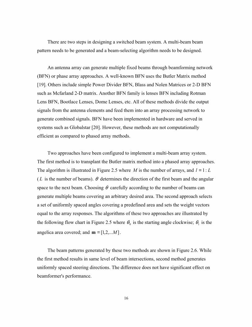
There are two steps in designing a switched beam system. A multi-beam beam
pattern needs to be generated and a beam-selecting algorithm needs to be designed.
An antenna array can generate multiple fixed beams through beamforming network
(BFN) or phase array approaches. A well-known BFN uses the Butler Matrix method
[19]. Others include simple Power Divider BFN, Blass and Nolen Matrices or 2-D BFN
such as Mcfarland 2-D matrix. Another BFN family is lenses BFN including Rotman
Lens BFN, Bootlace Lenses, Dome Lenses, etc. All of these methods divide the output
signals from the antenna elements and feed them into an array processing network to
generate combined signals. BFN have been implemented in hardware and served in
systems such as Globalstar [20]. However, these methods are not computationally
efficient as compared to phased array methods.
Two approaches have been configured to implement a multi-beam array system.
The first method is to transplant the Butler matrix method into a phased array approaches.
The algorithm is illustrated in Figure 2.5 where M is the number of arrays, and Ll :1=
( L is the number of beams). θ determines the direction of the first beam and the angular
space to the next beam. Choosing θ carefully according to the number of beams can
generate multiple beams covering an arbitrary desired area. The second approach selects
a set of uniformly spaced angles covering a predefined area and sets the weight vectors
equal to the array responses. The algorithms of these two approaches are illustrated by
the following flow chart in Figure 2.5 where 0θ is the starting angle clockwise; 1θ is the
angelica area covered; and ],...2,1[ M=m .
The beam patterns generated by these two methods are shown in Figure 2.6. While
the first method results in same level of beam intersections, second method generates
uniformly spaced steering directions. The difference does not have significant effect on
beamformer's performance.

17
S1, S2, . , SM ant #1 ant #2 . . . x1 xN w1,1
* . . . w1,N* . . . wN,1
* . . . wN,N*
q1 q1 Si,1 y1 yN . q2 q2 Si,2 r1 qM . . . qM
Si,M r2 . . . rM
Fig 2.4 Switched Beam System Block Diagram
There are two ways to select a particular beam from the set to serve a certain user.
One is to use a threshold and start selection from the first beam (set of weights).
Whenever the output from the cross correlators ( miS , in Figure 2.4) is larger than the
threshold, the corresponding weights iMi ww ,...,1 are chosen. A second method is to choose
the weights that generate the strongest output from the cross correlators. Selection by
threshold will somewhat reduces the beamforming time.
Freq. D/C & Demod
Freq. D/C & Demod
Cross Correlator
Cross Correlator
Cross Correlator
Beam Selector
Beam Selector
Beam Selector
Cross Correlator
Cross Correlator
Cross Correlator

18
(1) (2)
Fig 2.5 Multi-beam Generating Algorithms
Fig 2.6 Multi-beam Patterns of Switched Beam Systems
Mw 2'1 =
)1
121(8
'1
', −
−−××+=MlMiww li θ
)4,mod( ''' Mll ww =
Mll 2'' π×= ww
φπ sin)1( −= mw jl e
Ll 1
10−+= θθφ

19
2.3 Adaptive Beamforming
Adaptive beamformers are able to automatically optimize the beam pattern by
adjusting the controlling weights of the array elements to satisfy a prescribed objective
function [6]. Unlike fixed beam systems, not only the steering directions but also the
entire beam patterns are automatically formed during the adaptation process. Adaptive
beamformers can tract the desired user signal and/or put nulls toward interferes signals
provided that there are more array elements than interferers. Adaptive beamforming
algorithms can be categorized into non-blind and blind algorithms. Non-blind algorithms
use training signals while blind algorithms explore prior knowledge of certain properties
of the desired signal.
2.3.1 Algorithm Basics
Many algorithms have been developed for adaptive beamforming. However, all
these algorithms share the same foundation and follow basic approaches each of which
include a criteria and an adaptive process. Criteria for optimal weights are summarized in
Table 2.1 [6].
In Table 2.1, )( HE xxR = , )( Hu E uuR = , )( H
s E ssR = , )()( * ttdE xr = and
*,,, ddwv,su,x, , are array output, interference signal, desired user signal, array response,
controlling weights, desired signal and reference signal, respectively. Solutions for all
three types of criteria can be generalized as the Wiener solution where β is a scalar
coefficient.
Adaptive algorithms are used to resolve the matrix inverse and eigenvalue problems
existing in seeking the Wiener solution. It is important that the algorithm designed
converge fast and incur less computational complexity. Three commonly used algorithms

20
[6] are shown below, while others such as by neural networks are also presented in
literature.
Table 2.1 Criteria for Optimal Weights
Criteria Minimum Mean Square (MMSE)
Minimum Signal to Interference Ratio (MSIR) Minimum Variance (MV)
Methods
Minimize the distance between the reference signal and the array output
2*2 )]()([)( ttdt H xw−=ε
Maximize the signal to interference ratio
wRwwRw
uH
sH
SIR =
Minimize the output noise variance
wRwwRw uH
sHyVar +=)(
Equation 0
22))(( 2
=+−=
∇Rwr
w tE ε wwRR max
1 λ=−su
0
])1[21(
=−=
−+∇
vwR
vwwRww
β
β
u
Hu
H
Solution vRv
vRw
12
2
1
)(1)(
−
−
+=
=
uH
uopt
tdEtdEβ
β
optH
uopt
SIRtdE wv
vRw
)( 2
1
=
= −
β
β
vRv
vRw
1
1
−
−
=
=
uH
uopt
gβ
β
Least Mean Squares Algorithms employ simple recursive equations (2.8) based on
the equation of MMSE in Table 2.1.
)]([)(
))](([21)()1( 2
nn
nEnn
Rwrw
ww
−+=
−∇+=+
µ
εµ (2.8)
Instant estimates of R and r ( )()()( nnn HxxR =∧
and )()()( * nndn xr = ) are used such
that
)()()(
)]()()()[()()1(*
*
nnn
nnndnnn H
εµ
µ
xw
wxxww
+=
−+=+∧
∧∧∧
(2.9)

21
The LMS algorithm is simple but its convergence depends on the ratio of the largest
eigenvalue to the others, especially the second largest one. Also, the accurate estimation
of R and r depends on the stationary properties of the signals.
Direct Sample Covariance Matrix Inversion (DSCMI) employs the direct inversion
of the covariance matrix R in MMSE equation in Table 2.1. R and r are estimated in the
same way but from a block of samples. The least square solution will then be applied to
∧−∧∧
= rRw1
∧∧
−= rwR opte (2.10)
The DSCMI method converges faster than LMS but with higher complexity and
finite precision problems causing instability when inverting a matrix.
Recursive Least Square (RLS) uses the weighted sum instead of a square window to
estimate R and r by the equation below where 10 << γ is the weighting factor
)()()1()( nnnn HxxRR +−=∧∧
γ (2.11)
)()()1()( * nndnn xrr +−= γ (2.12)
The weight can be updated as
)]1()()()1([)( 1111 −−−= −−−− nnnnn RxqRR γ (2.13)
)()1()(1)()1()( 11
11
nnnnnn H xRx
xRq−+
−= −−
−−
γγ (2.14)
)]()1()()[()1()( * nnndnnn H xwqww −−+−=∧∧∧
(2.15)
The RLS algorithm replaces the inversion of the covariance matrix )(nx by scalar
division and is an order of magnitude faster than the LMS algorithm [6].
22
2.3.2 Blind Algorithms
Blind algorithms do not need an explicit training sequence but rather generate their
own references. Some commonly seen blind algorithms are summarized in this section
with specific algorithms suitable for CDMA systems addressed in the next section.
DOA estimation algorithms such as MUSIC [22] and ESPRIT [23] use prior
knowledge of array response or array manifold to estimate the DOA. Performance of
DOA estimation algorithms depends on the accuracy and reliability of this knowledge.
Furthermore, these algorithms can only estimate DOA up to the number of the array
elements, a major disadvantage for application in cellular environments where multipath
exists and the number of users is far greater than the number of array elements.
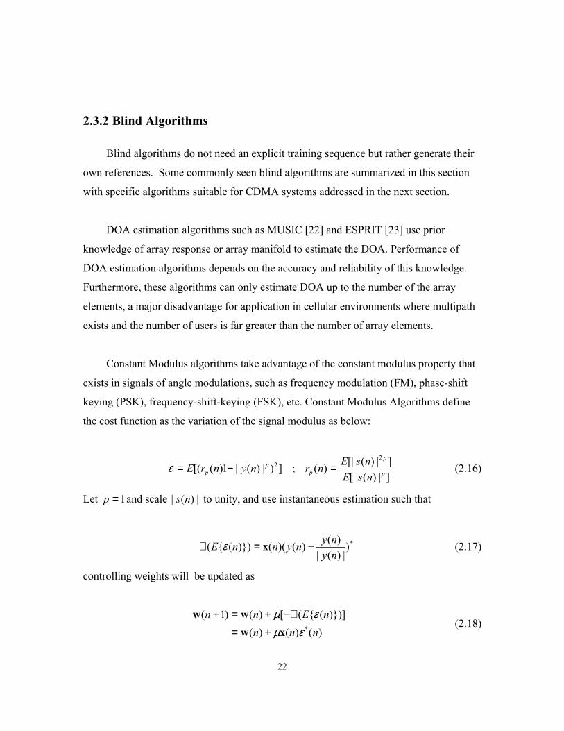
Constant Modulus algorithms take advantage of the constant modulus property that
exists in signals of angle modulations, such as frequency modulation (FM), phase-shift
keying (PSK), frequency-shift-keying (FSK), etc. Constant Modulus Algorithms define
the cost function as the variation of the signal modulus as below:
])|)(|1)([( 2pp nynrE −=ε ;
]|)([|]|)([|)(
2
p
p
p nsEnsEnr = (2.16)
Let 1=p and scale |)(| ns to unity, and use instantaneous estimation such that
*)|)(|
)()()(())((nynynynnE −=∇ xε (2.17)
controlling weights will be updated as
)()()(
))](([)()1(* nnn
nEnnεµ
εµxw
ww+=
−∇+=+ (2.18)

23
where |)(|
)()()(nynynyn −=ε (2.19)
It is easy to see that the updating equation is similar to that of LMS methods except that
the reference for CMA is implicit as the constant modulus of the signal.
The CMA algorithm does not require an explicit reference signal. However its
performance depends on the constant amplitude of the desired signal. In reality this can
not be true as the signals are subject to multipath effect and imperfect power control.
In Decision-Direct Algorithms (DDA), the beamformer output is demodulated and
the decision-maker makes a decision based on the demodulated signal. A reference signal
is generated by modulating the decision. The process is shown in Figure 2.7 below [6].
Fig 2.7 Reference Generation in Decision Direct Algorithm
DDA updates the weights by adaptive algorithms such as LMS. DDA and CMA
cannot guarantee the convergence of the adaptive process because of the non-convex
property of the cost function.
Demod Decision
Modulation
)(ty Beamformer
output
d*(t) Reference
signal
24
2.3.3 Blind Algorithms in CDMA Systems
Signals in CDMA systems have some properties that favor certain types of adaptive
beamforming algorithms. These algorithms include Maximum Power Lagrange (MPL)
algorithm [24] and Code Gate Algorithm (CGA) [25].
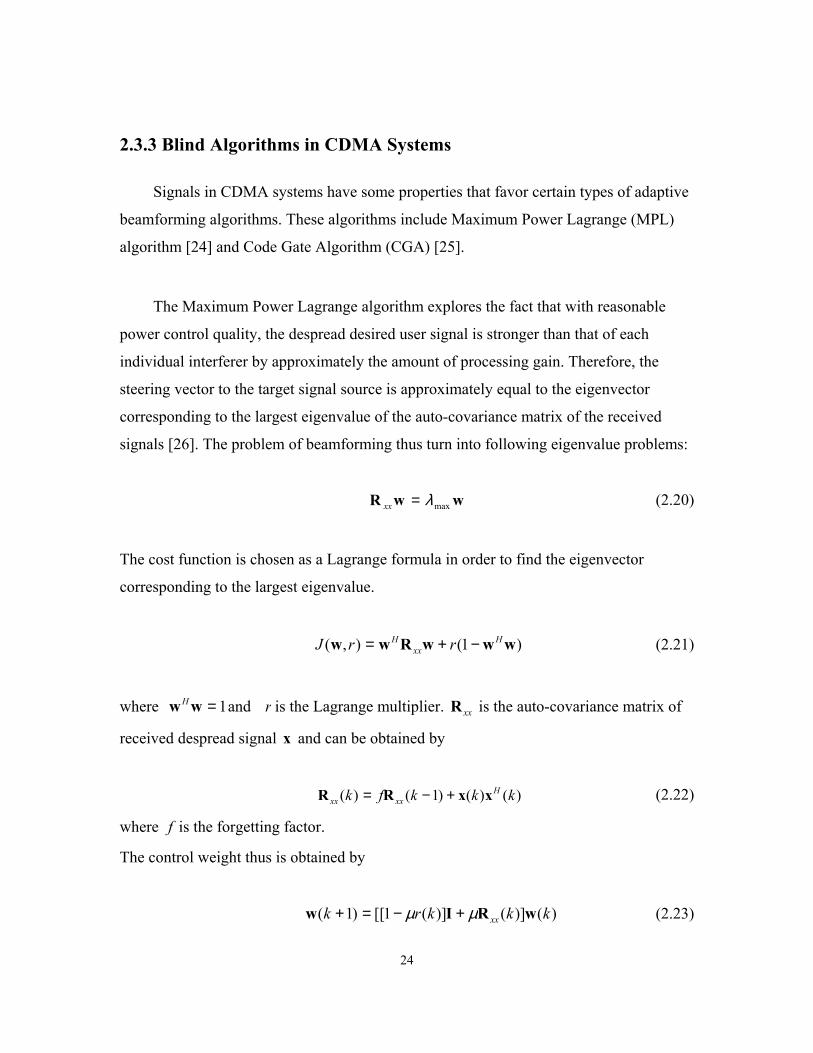
The Maximum Power Lagrange algorithm explores the fact that with reasonable
power control quality, the despread desired user signal is stronger than that of each
individual interferer by approximately the amount of processing gain. Therefore, the
steering vector to the target signal source is approximately equal to the eigenvector
corresponding to the largest eigenvalue of the auto-covariance matrix of the received
signals [26]. The problem of beamforming thus turn into following eigenvalue problems:
wwR maxλ=xx (2.20)
The cost function is chosen as a Lagrange formula in order to find the eigenvector
corresponding to the largest eigenvalue.
)1(),( wwwRww Hxx
H rrJ −+= (2.21)
where 1=wwH and r is the Lagrange multiplier. xxR is the auto-covariance matrix of
received despread signal x and can be obtained by
)()()1()( kkkfk Hxxxx xxRR +−= (2.22)
where f is the forgetting factor.
The control weight thus is obtained by
)()]()](1[[)1( kkkrk xx wRIw µµ +−=+ (2.23)

25
where µ is the adaptive gain factor that determines the convergence speed.
Like other approaches such as CGA, a simplified version of MPL method sets f to
zero, i.e. uses instant estimation to reduce the complexity..
The CGA algorithm is based on maximum total signal to interference and noise
ratio (TSINR) shown in Table 2.1 and has the solution as the eigenvector of the following
equation
wwRR max1 λ=−
su (2.24)
It is natural to use the despread array output as the reference to the signal of the
desired user, and from it and by proper process generate the estimation of interference.
The reference acquiring process is illustrated in Figure 2.8 where ic is the spreading code
for the ith user. The reference to the desired signal comes directly from a low pass filter
fed with the despread array outputs.
∫+
+−= ib
ib
nT
Tn ib
i dttxT
nτ
τ)1()(1)(y (2.25)
The interference reference can be obtained by subtracting the desired reference signal
from the total signal as
)()()( nnαn yxu β−= (2.26)
The general eigenvalue problem as Equation 2.24 can be solved by adaptive algorithms
such as Generalized Lagrange Multiplier Method (GLM), Adaptive Matrix Inversion
Method (AMI) or others like those discussed in Section 2.3.1.

26
Fig 2.8 CGA Beamformer Block Diagram
The CGA algorithm is designed to take advantage of the existing despread signal in
the CDMA receiver, which simplifies the reference acquisition process. However, the
estimation of α and β in Equation 2.26 may not be straightforward and often degrades
algorithm performance. Indirect matrix inversion operations also face problems such as
singularity of the matrix and finite precision of processors. These problems degrade the
performance of the optimal beamformer such that in reality a sub-optimal beamformer
may outperform an optimal beamformer [25].
If the interference and noise signal )(nu is spatially and temporally white, we can
maximize the beamformer output due to a desired user signal by following sub-optimal
CGA equation
wwR maxλ=yy (2.27)
LPF
HPF
Ci
LPF
HPF
Ci
LPF
HPF Ci
M
iyy ,R
iuu ,R
iHi yw
iiiyyiuu wwRR max,1, λ=−
1y
u
Beamformer Output
iw
1,ix
2,ix
Mix ,

27
which is exactly the same as Equation 2.20. This illustrates that sub-optimal CGA
problem and solution are exactly the same as those of MPL.
2.4 Complexities and Hardware Requirements of CDMA SA
Algorithms
Ideal smart antenna algorithms should achieve interference reduction with low
computational complexity and hardwire requirements subject to the application
environment. CGA and sub-optimal CGA (or MPL) are designed for CDMA systems.
Their complexity and hardware requirements are compared to the switched beam
systems.
Figure 2.9 illustrates the computational process and complexity of CGA, sub-
optimal CGA and switch beam algorithms. Variable N in Figure 2.9 is the number of
array elements used and also represents N complex multiplication when referring to
computational complexity. We can conclude that CGA will have approximately O(8N)
complexity per iteration and Sub-Optimal CGA will have O(5N) complexity per iteration.
It is worth noticing that the complexity of the adaptive algorithms is independent to the
number of users in the system. It is also easy to see that the switch-beam system will have
O(N*M) complexity where M denote the number of users. The complexities of the
algorithms are shown in figure 2.10 assuming that the adaptive process converges after 4
iterations.
Hardware requirements do not differ much for all three algorithms. The number of
RF fronts and cross correlators required is equal to the number of array elements and
independent of smart antenna algorithms. Requirement on DSP is based on the
computational complexity shown above. In addition, CGA requires N high pass and low
pass filters while sub-optimal CGA requires N low pass filters only. Switched beam

28
Fig 2.9 CGA and Sub-Optimal CGA Computing process
Fig 2.10 Complexity of the Smart Antenna Algorithms
)0(w Initial guess
Lagrange Multiplier γ
xwuwxuuu
H
H
H
H
z ==
==
δξα
;
aacbb
zzczb
a
−−=
+=+=
=
2
*22
*2
22
)Re(2||||)Re(||
||
γ
ξδξµξδµααδ
αδµ
O(4N)
Update Weight w
||||/)(
)(
wwwuxw
wuuwxxww
=−+=
−+=δγµγµ
z
HH
O(3.5N)
)0(w Initial guess
Array Output xw Hy =
x New signal vector
Array output xwHy =
O(N)
Lagrange Multiplier γ
aacbb
yycyb
−−=
+=+=
=
2
22
2
||||2||||1||||
γ
µµµα
Update Weight w
||||/]1[
wwwxww
=+−= Hyµµγ
O(3.5N)

29
systems, on the other hand, need an additional signal selector. These additional
requirements can either be satisfied by employing specific hardware or increasing
computational load on DSP.
It can be concluded from the above discussions that from the implementation point
of view, the sub-optimal CGA algorithm is better than switched beam systems.
Comparison of performance and other aspects of switch-beam and adaptive arrays will be
given in the next section and chapter 5.
2.5 Application Issues of SA in CDMA systems
2.5.1 Performance and Beam Pattern Performance of the smart antenna systems is closely related to the beam pattern.
Theoretically, it is possible to maximize the desired signal power and at the same time
completely null out all the interfering signals if the signal satisfies certain conditions
illustrated by the following equations.
wRwsw sHH
s E == || 22δ (2.28)
wRwuw uHH
u E == || 22δ (2.29)
If 0|||| =uR , it is possible to choose a certain w such that 02 =uδ . Meanwhile, if
there is still freedom in choosing w , it is possible to maximize 2sδ at the same time. The
following examples illustrate how the beamformer maximizes the desire signal gain and
nulls out the interferers.

30
Example 1 [6]:
Assuming that the desired signal )(ts arrives from broadside and the interferer from
6π . The beamformer outputs due to the desired signal and interferer respectively are
))(()(
))(()(
22
1
21
ww
wwπj
i
d
etity
tsty
+=
+= (note: 2)6sin(2 ππ
λπ =d ) (2.30)
To maximize the desired signal output and null out the interferer, 21,ww should satisfy
0]Im[]Im[1]Re[]Re[
21
21
=+=+
wwww
and 0]Im[]Im[0]Re[]Re[
21
21
=+=+
wwww
jj
(2.31)
and the solution is 5.05.01 j−=w , 5.05.02 j+=w .
Example 2:
Assuming 21,uu are two interferers and ],1[],,1[ 21 vv are two array responses
according to AoA of 21,uu , the covariance matrix is
))(())(((||||
[(
2211212211212
22112
21
221121221121
vuvuuuEvuvuuuE)vuvE(u)uuE
)]vuv),(uu[(u)]vuv),(uuuE
uu
Huu
++++−++=
++⋅++=
R
R(2.32)
It is somewhat difficult to draw a general condition under which the above equation
holds, but two case studies can illustrate the idea.
If there is just one interferer as 1u , 0|||| =uuR which means that one interferer can
always been canceled by the antenna array. Another case is that two interferers with

31
identical AoA i.e. 21 vv = would also give 0|||| =uuR , which shows that two interfering
signals from the same direction can always be canceled by antenna arrays.
However, possibility of complete null all interferers (optimum beamforming)
depends on the interference signals, array response and how many degrees of freedom the
controlling weights have.
Another issue concerned with join maximization of the desired signal and nulling
the interferers comes from the process of getting w . Although theoretically blind
beamforming algorithms will automatically generate the beam patterns that completely
null out the interferers if possible, it is generally not easy to get the optimal result when
uuR is singular.
Furthermore, if the interference and noise signal is spatially and temporally white,
there is no gain by placing nulls toward the interferers in addition to pointing the main
beam to the desired signal. It is obvious that because of the whiteness, the gain from
nulling out one interferer will be lost since another interferer may be amplified. In
addition, there is no way to completely simultaneously null out all the interferers by
adjusting the beam patterns if the number of array elements is less than the number of
interferers with distinct incident angles. The optimal algorithms will collapse [27] in such
situations. It is possible to null out major interferers whose number is less than that of the
array elements. However in a cellular system where interferers usually outnumber array
elements many times, it is not quite clear whether the scheme will bring real benefits after
paying the price of more complex processing.
Generally speaking, interference signals are spatially white when traffic comes from
all the directions such as in the center of an urban area. On the other hand, it is unlikely to
be spatially white in suburban areas when traffic flows mainly along highways and when
the area around the base stations is not symmetrically populated. Similar conclusion

32
about the performance comparison of optimal and sub-optimal approaches can be found
from reference [28].
If infinite processing gain is assumed, it is easy to find that the weights generated by
sub-optimal CGA algorithm (Equation 2.27) correspond to the natural array response of
the desired user signal scaled by a factor of N , where N is the number of array
elements. Using natural array response of the desired user instead of sub-optimal CGA
would therefore slightly improve the performance. It is also worth noticing that sub-
optimal CGA is a phase array approach while optimal beamforming generally is not
(since the amplitude and the phase of the signal from array elements are both changed
while, however, the norm remain the same).
2.5.2 AOA Spread and 2-D RAKE Radio channel characteristics differ in densely populated urban areas with micro or
pico-cells from that in large suburban areas with a macro cell environment. For a macro
cell environment, there is likely to be a line of sight (LOS) component of the signal and
the angular spread of the signal is small. In micro- or pico-cell environments, it is less
likely to have a LOS component and the angular spread tends to be large. Models of AoA
spread can be found in the literature, e.g. [29].
Another concern is whether the system is narrowband or wideband. For a
narrowband system, all multipath components arrive with very small delay compared to
the chip period (also called correlated) and cannot be resolved by temporal RAKE
receivers. In the mean time, it is more likely that the multipath components will have a
small angular spread because otherwise large delay shall arise. In wideband systems, all
the multipath components arrive with sufficient separation (uncorrelated) and can be
resolved by temporal RAKE receivers.

33
Smart antenna algorithms yield different performances in different environments.
For wideband systems, 2-D RAKE receiver can be employed with either adaptive array
or switched beam antenna. Table 2.2 below [30] shows the performance measured in
maximum number of users supported at outage probability of 10%
( %10)10Pr( 2 <>BER ) with perfect power control and processing gain equal to 31. SB
stands for switched beam and OSF for optimal spatial filtering which is another term for
adaptive array. Geometrically Based Single Bounce (GBSB) multipath model is used to
compute the table.
Table 2.2 Performance of Switched Beam and Adaptive Array
(with uncorrelated multipath components)
Number of user supported at Pr(BER> 10-12)<10% Number of Multipath
Components Omni M=6,
SB M=6, OSF
M=12, SB
M=12, OSF
1 14 31 >31 >31 >31 6 6 20 28 20 >31 10 4 15 23 20 29 20 1 11 14 20 24 30 0 6 10 13 20
(with correlated multipath components)
Number of user supported at Pr(BER> 10-12)<10% Number of Multipath
Components Omni M=6,
SB M=6, OSF
M=12, SB
M=12, OSF
1 14 31 >31 >31 >31 6 0 16 >31 >31 >31 10 0 6 >31 25 >31 20 1 10 >31 21 >31 30 0 12 >31 14 >31
It can be seen that for correlated multipath components, switch beam system is not
able to offer performance comparable to adaptive array systems even with more

34
elements, especially when the number of multipath components is large. It is clear that
switched beam systems do not have the same ability as adaptive array in resolving
multipath with small AoA spread.
In the wideband case, even for a large number of multipath components, switch
beam system can still offer performance comparable to adaptive arrays. By a reasonable
increase in elements, it can even outperform the adaptive array, but of course the
computation complexity also increases.
Furthermore, the temporal RAKE combining possible in wideband systems will
give major utilization to multipath diversity (temporal diversity). The spatial RAKE
combining will further explore the angular diversity of the multipath and improve the
combining effect. However, it may not bring significant difference to the performance
compared with 1-D RAKE receiver. For the same reason, the performance difference
between switched beam and adaptive array due to spatial RAKE combining is not
substantial.
WCDMA system is wideband because of its high chip rate. Assuming spatial and
temporal whiteness of the interfering signal, there would be some but small difference in
performance analysis between 2-D RAKE and conventional RAKE receiver with either
switched beam or adaptive array. In a macro-cell environment, it is still a wideband
system even if the angular spread is small. Employing temporal RAKE receiver thus
reduces the need for spatial filtering in combating multipath effect. It is reasonable to
assume no angular spread of multipath components in both micro and macro cell
environments in a simulation study on switched beam and adaptive array performance,
which cuts down the complexity but still generating results with enough fidelity.
35
2.5.3 SA Applications in CDMA Systems For downlink transmitting a beamformer can point a beam to the desired mobile and
reduce the transmitting power. The interference to other mobiles reduces accordingly
both because the transmission is along a specific direction and because the power is
reduced. Downlink beamforming is thus capable of improving the received signal quality
at mobiles as well as expanding and reshaping base station coverage area.
For uplink transmitting, there are four ways to utilize antenna arrays to improve
performance. The major improvement comes from co-channel interference reduction
through beamforming gain. Second is fading suppression via exploring angular diversity
by pointing the beams to different multipath components and combining the output. The
third method that also combats multipath fading is exploring spatial diversity from the
separated antenna array. Finally SNR improvement is achieved when adding signals from
several antenna elements multiplies the signal power over noise. Only co-channel
interference reduction through beamforming will be studied in later part of the thesis. A
temporal RAKE receiver will be used to mitigate the fading effect.
36
Chapter 3
Radio Resource Management
Radio Resource Management (RRM) is very important for efficient usage of radio
resources and for guaranteeing Quality of Service (QoS). RRM manages and controls the
usage of radio resources such as transmitting power, available spectrum and hardware
(equipped channels). Although the number of equipped channels (modulation and
demodulation modules) can limit the capacity of the system, the focus in this thesis will
be on interference-based radio resource management. A brief discuss on resource
management in TDMA/FDMA systems is given as an introductory complement followed
by detail discussion on RRM in CDMA systems.
3.1 Introduction to Resource Management
Resource management in TDMA/FDMA and CDMA systems has the same goal yet
takes different mechanisms because of different reuse factors in this two type of systems.
In TDMA/FDMA systems available spectrum is divided into channels and assigned to
different users in one cell and is reused in cells with a certain distance. Unlike
TDMA/FDMA systems, CDMA systems assign entire available spectrum to every user in
the cell and reuse it in all the neighboring cells. This means that all the users in the
covered area share a same available broadband channel. Resource management for
CDMA systems thus can facilitate some new functions such as soft handover and macro
diversity to enhance the performance.
RRM consists of power control, handover, call admission control, channel

37
assignment and reservation as well as load control and packet scheduling. Load control
and packet scheduling are typically addressed in radio network planning and are not
discussed in this thesis.
Power control refers to controlling the transmitting power so that the signals will
reach the receivers with enough energy while generate as little co-channel interference as
possible to other signals. Handover happens when a mobile moves from one cell to
another. Handover algorithms will ensure that the old serving base station is replaced by
a new base station while trying to minimize the effect on the ongoing communication
process. Call admission, channel assignment and channel reservation determine how the
calls are accepted and resources are assigned with the objectives of minimizing the
overall interference level, reducing the outage probability for ongoing calls and exploring
the capacity of the system to its fullest extent possible.
3.2 Resource management in TDMA/FDMA systems
Power control error usually is not as crucial in a TDMA/FDMA system as in
CDMA systems. Power control in TDMA/FDMA systems usually takes into account the
long-term path loss variation without instantaneous fading effects. Power control in a
TDMA/FDMA system may be implemented using centralized or distributed controllers
based on either received power level or signal to noise and interference ratio. However, a
centralized controller is not feasible because of the huge overhead for information
transferring and processing as well as the corresponding delay. An SIR based distributed
power control algorithm can be found in [18]. The SIR for a given link can be written as
i
M
jjji
iM
ijj
ii
ji
ii
PPZ
P
PGGP
−==Γ∑∑
=≠ 1,
,
, (3.1)

38
where iP is the i th mobile power; jiG , is the path gain of the i th mobile to the j th base
station and iijiji GGZ ,,, = . It has been shown in [18] that the largest iΓ is achieved by
choosing power control vector P ( Nppp ,,, 21 K ) equal to the eigenvector corresponding
to the largest eigenvalue maxλ of jiZ , . And by doing so, the largest iΓ is also the smallest
iΓ so that the SIR is balanced. Several distributed algorithms driving the iΓ to its
balanced value are illustrated below [18] where tΓ is the target SIR
)11( 11
−−
Γ+= K
i
Ki
Ki PP κ
1
1
−
−
Γ= K
i
KiK
iP
P ξ (3.2)
11
−−
ΓΓ
= Ki
tKi
Ki PP
TDMA/ FDMA employs a hard handover algorithm when mobiles move from one
cell to another. Each base station monitors the signal strength of the mobiles it serves and
that of other mobiles in its neighboring cells, and transfers the information to a mobile
switching center (MSC). When the MSC detects a pilot signal drop below the handover
threshold for a certain period of time, it initiates the hand off process. Second generation
mobile systems such as GSM use mobile assisted handover (MAHO) where mobiles
monitor the pilot signal strength from their neighboring cells. A mobile station initiates a
handover process when the signal strength from its serving base station drops below the
signal strength from another base station by a certain amount for a period of time.
Handover parameters include handover hysteresis defined as drophandoff PP −=∆ and
waiting time wT . These parameters must be set carefully to provide enough time for the
handover operation while avoiding unnecessary handovers due to temporary fading
effects and non-crossing mobile moving at the boarder. Dwell time, the time when a call
remains within a cell, is one statistics helpful to set the hysteresis. Other statistics drawn
39
from the signals can also provide information such as speed of the vehicles to assist in the
handover process.
Channel assignment for TDMA/FDMA systems can be classified into fixed channel
assignment (FCA) and dynamic channel assignment (DCA). In FCA scheme, channels of
fixed number are assigned to a cell and are reused by a certain pattern. FCA is not
adaptive to traffic changes. In the DCA scheme, all channels belong to a set from which
any can be assigned to a mobile. The DCA scheme is traffic adaptive since the number of
channels assigned to a cell is not fixed. DCA algorithms are usually based on co-channel
interference. The maximum SIR (MSIR) algorithm selects an unused channel with
maximum SIR to serve the new call. Channel segregation lists the channels by their
selectability and chooses the serving channel by following pre-established rules.
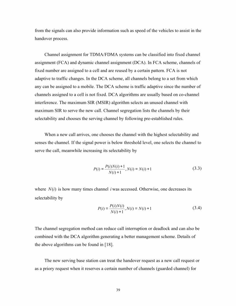
When a new call arrives, one chooses the channel with the highest selectability and
senses the channel. If the signal power is below threshold level, one selects the channel to
serve the call, meanwhile increasing its selectability by
1)()(,1)(
1)()()( +=+
+= iNiNiN
iNiPiP (3.3)
where )(iN is how many times channel i was accessed. Otherwise, one decreases its
selectability by
1)()(,1)()()()( +=
+= iNiN
iNiNiPiP (3.4)
The channel segregation method can reduce call interruption or deadlock and can also be
combined with the DCA algorithm generating a better management scheme. Details of
the above algorithms can be found in [18].
The new serving base station can treat the handover request as a new call request or
as a priory request when it reserves a certain number of channels (guarded channel) for

40
handover purposes only. If there is no channel available, a new call is rejected. If there is
no reserved channel available, the handover request is rejected and the call is dropped
(handover failure). Sometimes, a reserved channel can be borrowed to serve a new call
based on careful consideration of handover statistic so that such borrowing will not
increase handover failure rate.
3.3 Power Control in CDMA Systems
The performance of CDMA systems depends greatly upon power control. Since all
the mobile stations share the same broadband channel in a CDMA system, a single high
power transmitter will severely degrade performance on all other ongoing
communications. A CDMA system is more vulnerable to fading due to the same reason.
Power control in CDMA therefore must keep signals received at the BS from all the users
served in the cell as close as possible to the same level. Fast power control thus is
indispensable for combating fading effects. Meanwhile power control should also keep
the transmitting power as low as possible to save energy and reduce interference under
the condition of satisfying performance requirements.
CDMA power control schemes should first equalize the power levels at the BS of
the received signals from local (within the cell) mobile stations, and then balance the SIR
among cells over the coverage area. CDMA power control schemes that only achieve the
first goal are power level based while schemes also balancing SIR are SIR based. Power
level based PC algorithms can be described similarly as the SIR based algorithms except
that a target signal power level ettPS arg is set instead of a target signal to noise ratio
ettSIR arg . A detailed description of a power control algorithm is given below based on the
WCDMA proposal, which is a SIR based algorithm.
In the WCDMA frequency division duplexing (FDD) scheme [31], two loops of
power control mechanism are suggested for ordinary up-link transmission. Outer-loop
power control sets the SIR target ( ettSIR arg ) according to the bit error rate (BER) or frame

41
error rate (FER) and QoS requirements. The inner-loop power control function adjusts
the UE transmitting power so that the signal-to-interference ratio (SIR) is maintained at a
given SIR target ( ettSIR arg ). Inner-loop fast power control is discussed in the following
part of the thesis.
The serving cells BS (cells in the active set) should estimate signal-to-interference
ratio ettSIR arg of the received up-link DPCH (dedicated physical channel). The serving
cells BS then generates TPC commands and transmits the commands once per slot
according to the following rule:
If estSIR > ettSIR arg , the TPC command to transmit is "0",
If estSIR < ettSIR arg , the TPC command to transmit is "1".
Upon receipt of one or more TPC commands in a slot, the user equipment (UE)
derives a single TPC command cmdTPC . The UE combines multiple TPC commands if
more than one is received in a slot. Two algorithms are suggested to be supported by the
UE for deriving a cmdTPC . Which of these two algorithms is used is determined by a UE-
specific higher-layer parameter, "PowerControlAlgorithm" (PCA), and is under the
control of the UTRAN. The first algorithm is described below.
When a UE is not in soft handover, only one TPC command will be received in each
slot. In this case, the value of cmdTPC shall be derived as follows:
- If the received TPC command is equal to 0, then cmdTPC for that slot is 1.
- If the received TPC command is equal to 1, then cmdTPC for that slot is 1.
When a UE is in soft handover, multiple TPC commands may be received in each
slot from different cells in the active set. The UE conducts a soft symbol decision iW on
each of the power control commands iTPC , where i = 1, 2, , N, with N greater than 1

42
the number of TPC commands from radio links of different radio link sets. The UE then
derives a combined TPC command, cmdTPC , as a function of all the N soft symbol
decisions iW , that is, cmdTPC = γ ( 1W , 2W , NW ), where cmdTPC can take the values 1
or -1. The function γ shall fulfill the following criteria
If the N iTPC commands are random and uncorrelated with equal probability of
being transmitted as "0" or "1", the probability that the output of γ is equal to 1 shall be
greater than or equal to 1/(2N), and the probability that the output of γ is equal to -1 shall
be greater than or equal to 0.5. Furthermore, the output γ of shall be equal to 1 if the TPC
commands from all the radio link sets are reliably "1", and the output of γ shall be equal
to 1 if a TPC command from any of the radio link sets is reliably "0".
It is very important to set a proper target ettSIR arg that meets the QoS requirement
and at the same time is feasible. In a balanced SINR power control scheme, the target
ettSIR arg should not exceed the upper limit maxSIR determined by the number of users in
the system. Otherwise the scheme will fail. The achievable balanced target maxSIR is not
a function of radio resources but of the number of users and the interference reduction
capability (spreading gain in the system). However, SINR based power control should set
the transmitting power of every mobile to its minimum satisfying the performance
requirement rather than the maximum value regardless of the system load pgc / (see
Equation 3.5). It also balances the SINR and reduces interference accordingly. As a
result, the system capacity is further increased. ettSIR arg is set at RNC by jointly
considering the current system load and the QoS requirements. The following example
shows how power control works to reduce the transmitting power in a single cell [33].
NPpgc
PSIR ett
+=arg ;
pgcSIR
SIRNP
ett
et
arg
arg
1−
×= (3.5)

43
where P is the received power from one mobile, N is the power of white noise, c is the
number of interferers (number of user deducted by 1), pg is the processing gain. It is
obvious that no matter what P is, ettSIR arg cannot exceed pgc / . Under this condition,
Figure 3.3 below shows the power level necessary to achieve certain SIR with the
increase of the system load pgc / .
It is clear from Figure 3.1 that pursuing a high ettSIR arg close to its upper limit
requires a high level of transmitting power. Exceed power is defined as the ratio of the
Fig 3.1 Transmitting Power vs. System Load
required power level with more than one interferers in the system to that with just one
interferer. The absolute value depending on the noise power level is )1( =+= cPPP excess .
It is difficult to set a target SIR and pursue a multi-cell SIR balancing because the
traffics in those cells vary. On the other hand, balancing the SIR can not improve the
performance considerably if the system loads in different cells are close to each other.

44
3.4 Handover in CDMA Systems
CDMA systems employ soft handover algorithms that enable uninterrupted
communications during the handover process. Since all the mobiles share a same
broadband channel, every mobile in the soft handover region can communicate to more
than one neighboring BS at the same time. When a mobile moves from one cell to
another, it does not have to drop the link to the old BS before establishing one to the new
BS. Soft handover provide a seamless handover process as well as macro-combining to
mobiles in handover region.
Both IS-95A and WCDMA handover algorithm use CPICH (common pilot channel)
pilot 0/ IEc (definition of 0/ IEc can be found in [1] p115) as the handover measurement.
Handover algorithm in cdmaOne (IS-95A) can be illustrated as:
Pilot
0/ IEb T_ADD T_DROP Time Neigbour Candidate Active Neighbor Set Set Set Set (1) (2) (3) (4) (5) (6) (7)
. Pilot strength exceeds T_ADD. Mobile station sends a Pilot Strength Measurement Message and transfers the pilot to the candidate set . Base station sends a Handover Direction Message. . Mobile station transfers the pilot to the active set and sends a Handover Completion Message. . Pilot strength drops below T_DROP. Mobile station starts the handover drop timer. . Handover drop timer expires. Mobile station sends a pilot Strength Measurement Message. . Base station sends a handover Direction Message. . Mobile station moves the pilot from the active set to the neighbor set and sends a Handover Completion Message.
Fig 3.2 IS-95A Handover Process

45
The range (T_DROP, T_ADD) or its corresponding area at the cell boundary is
called the soft handover region (SR). It is obvious that handover rate increases with the
increase of SR.
Handover algorithm in WCDMA [32] can be illustrated as ∆T ∆T ∆T Pilot
0/ IEbof cell 2 AS_Th+AS_Th_Hyst
AS_Th-AS_Th_Hyst AS_Rep_hyst Pilot
0/ IEbof cell 2
Pilot
0/ IEbof cell 2
Connected to Cell 1 Event 1A Event 1C Event 1B = add cell 2 = replace cell 1 = Remove cell 3 with cell 3
. If Meas_Sign is below (Best_Ss - As_Th - As_Th_Hyst) for a period of ∆T, remove the worst cell in the Active Set. . If Meas_Sign is greater than (Best_Ss - As_Th + As_Th_Hyst) for a period of ∆T and the Active Set is not full, add Best cell outside the Active Set in the Active Set. . If Active Set is full and Best_Cand_Ss is greater than (Worst_Old_Ss + As_Rep_Hyst) for a period of ∆T, add Best cell outside Active Set and Remove the worst cell in the Active Set.
Where
AS_Th: Threshold for macro diversity (reporting range); AS_Th_Hyst: Hysteresis for the above threshold; AS_Rep_Hyst: Replacement Hysteresis; ∆T: Time to Trigger; AS_Max_Size: Maximum size of Active Set. Best_Ss :the best measured cell present in the Active Set; Worst_Old_Ss: the worst measured cell present in the Active Set; Best_Cand_Ss: the best measured cell present in the monitored set. Meas_Sign :the measured and filtered quantity.
Fig 3.3 WCDMA Handover Process

46
WCDMA handover algorithm uses relative thresholds while IS-95A and IS-95B use
absolute thresholds. All of these algorithms depend on the accurate measurement of the
pilot 0/ IEc . 0/ IEc can be obtained by filtering, which smooth the fading effect at the
mobile station. Longer filtering periods will generate more precise measurement, but
increases handover delay.
3.5 Call Admission Control in CDMA Systems
Network needs to know whether there is enough resource available to accommodate
more users when a new call request arrives. Call admission control (CAC) must check
not only the availability of those resources but also the effect to the system from the
increased interference if the new call is admitted. A new call request must be denied if
the admission will degrade the quality of any ongoing communications to an
unacceptable level.
The total power received by a base station (current interference) can be used as the
current interference level. The CAC estimates the total interference level assuming that
the new call is admitted. The CAC rejects the call if the interference is higher than a
certain threshold. Radio Network Controller (RNC) obtains the estimated interference
levels from all of its cells and decides whether an incoming call be accepted or not. The
following CAC algorithm is based on [34], [35]. Assuming that the pilot from BS k is
the strongest and )(kh Ω∈ is a nearby BS, the algorithm can be described as follows.
The MS measures )(kPm and )(hPm , the received pilot strength from BS k and
BS h respectively. )(kP and )(hP are the transmitted pilot strengths at BS k and h
respectively. MS thus can compute the path losses as )(/)()( kPkPkl mm = and
)(/)()( hPhPhl mm = . The ratio of the path loses is )(/)(),( klhlkhL mmm = . BS
k periodically measures its reverse link kSIR and updates the target signal power )(kPt ,
while BS h measures hSIR and updates )(hPt . The information of kSIR , hSIR , )(kPt ,

47
)(hPt and ),( khLm is transferred to RNC. RNC determines whether to admit the new call
by the following rule.
The residue capacity R is estimated as
>Ω∈=
=otherwise ,0
;0)( if ),(or |)(min jRkjkjjRR (3.6)
where
Ω∈−−
=−
=
);( if ,
)()(),(
111
; if , 11
)(
kj
kPhPkhLSIRSIR
kjSIRSIR
jR
t
tm
hTH
kTH
(3.7)
If 0>R , the call can be admitted. Otherwise, it is rejected.
The SIR threshold tSIR is bounded by
1
, 1
10/
)()(),(101
−
≠∈ =
−
+×
+−+≤ ∑ ∑
hjj
n
i t
tm
ih
ijhhth
jijih
kPhPkhL
rr
RnSIRψ
ξζα
(3.8)
where mhr is the distance from mobile m to BS h , and mhξ represents the shadowing
effect. α is the path loss coefficient. hn is the current number of mobiles in cell h and
hR is the residue capacity.
3.6 Capacity Reservation/Channel Assignment in CDMA systems
Capacity (channel) reservation works together with CAC. Handover requests in
cellular systems are considered as having higher priority than new call requests since
dropping an ongoing call is more annoying than rejecting a new call. A certain amount of
resources must be reserved for handover.
48
An interference based channel assignment scheme for DS-CDMA cellular systems
is proposed in [35]. The scheme reserves capacity by setting up a handover interference
margin HIM . The algorithm is described below.
The bit energy to noise (including the interference) power spectral density ratio
0/ NEb is given by
WSNNRSNE
tb /)1(
)/(/ 0 ×−+×= α (3.9)
where N is the number of users in the cell; S is the received signal power; R is the bit
rate; W is the chip rate; tN is the thermal noise power spectrum density; and α is the
voice activity factor. Rearranging the equation and replacing S with NS , we have the
received signal power required for supporting N users in the cell as
0
0
/)/( where
)1(
)1(/
)/(
NERWG
NGWN
NNE
RWWNS
b
t
b
tN
α
α
=−−
×=
−−
×=
(3.10)
Including the interference from other cells oI , the total received power NP should be
)(1
1ot
NtN
IWNNG
GSNWNP
+×−+
+=
×+×= (3.11)
Thus,
N
otN
PNG
NG
IWNNG
GP
−−+=
+×+−+
+=+
1
)()1(1
11
(3.12)

49
This result is similar to that from SIR balanced power control (section 3.2) by that
SINR is kept constant and the target SINR ( 0/ NEb ) cannot exceed the system capacity.
In addition, the power required increases faster when the system load approaches the
system capacity.
TIM is defined as the total interference margin. TIM must be set to satisfy the target
SINR (or 0/ NEb ) with reasonable received signal power level. TIM can be set as
)( WNGTIM t ××= β where β denotes the maximum system load. Current interference
margin CIM is defined as equal to 1+NP in equation (3.12). Handover interference
margin HIM is defined as
NPRNG
NGHIM−−
−+= 1 (3.13)
where R represents the reserved capacity for handover. The capacity reservation scheme
(combined with CAC) is illustrated in Figure 3.4.
The capacity reserved by the above approach is fixed. More complex are adaptive
channel reservation schemes that adjust the reserved capacity according to handover
statistics.
An adaptive capacity reservation scheme proposed in [37] explores explicitly the
handover statistics. A new threshold T_RSRV below ADDT _ is set to measure the
likelihood that a mobile moves into the handover region. If the pilot from a neighboring
BS becomes stronger than T_RSRV but lower than ADDT _ , the mobile asks the
corresponding BS to reserve a channel for a possible handover. If the pilot becomes
stronger than ADDT _ , soft handover happens and the reserved channel is used. If the
pilot strength drops below T_RSRV for a predefined period, the reserved capacity is
released.

50
Fig 3.4 Channel Reservation Scheme
Another channel assignment scheme proposed in [38] reduces the soft handover
region by increasing the DROPT _ . Therefor, it not only releases the system capacity
used in actual handover activities but also the capacity reserved for possible handovers.
Read Interference level
NP , Calculate CIM, HIM
HIM > TIM
Handover ?
CIM > TIM
Admit the request
Reject the request
Yes No
NoYes
Yes
No

51
Chapter 4
Simulation Model on SA and RRM in CDMA Systems
This chapter describes the simulation model developed for studying smart antenna
and radio resource management in CDMA systems. The simulator is developed according
to the IS-95 and W-CDMA proposals, but with simplifications. The up-link scenario of a
multi-cell cellular system is simulated with omni-directional or smart antennas at the base
stations. This simulator consists of six integrated components including a mobility and
geographic model, an event simulator, a channel simulator, a signal processor, a smart
antenna processor and a resource management model.
4.1 General Description of The Simulator
Figure 4.1 illustrates the general block diagram of the simulator. A brief description
is given below about the functions of the blocks.
The mobility and geographical model generates the mobile speeds and the directions
according to certain probability distributions; calculates the mobile locations accordingly;
and calculates the path gains and AoA according to the mobile station (MS) locations.
The event simulator generates and schedules events including the call arrivals and call
departures, system status updates and mobile direction updates. The channel simulator
generates Rayleigh fading data; simulates multipath effect and generates received signals
from the channels. At the transmitters, the signal processor generates and spreads the
data; performs pulse shaping, and executes power control command. At the receivers, the

52
Information Flows: 1. MS locations 8. Transmitted signals 2. path gains, AoA 9. MSs Serving BS
15. Beamformer output of all received signals
3. MS locations 10. TPC 16. Handover requests 4 Path gains 11. MSs serving BS 17. Same as 15 5. Path gains (pilot strengths) 12. Array weights 18. Reserved capacity 6. MS IDs. 13. Beamformer output of pilots 19. Admission decision 7. Received signals 14. MSs serving BS
Fig 4.1 General Block Diagram of The Simulator
Mobility Model
Geographical Model
MS, BS location, Lognormal info
Channel Simulators
Call Arrival
SA Processors
Power Control
Handover
Capacity Reservation
Call Admission
MS Transmitter
BS receiver
MS,BS relation
Call Departure
Simulator Global Coordinator
6
2
1
4
5
3
1
2
3
4
5 6
7
8
9 10
11 12 13
14 15
16
17 18
1
4Model
Virtual Block for Information Diverting
Numbered Information Flow
General Model
Legend:
19

53
signal processor despreads the received signals and performs RAKE combining. The
smart antenna processor generates combining weights and processes received signals
accordingly. The resource management model generates power control commands,
performs handover processes, call admission control and capacity reservation.
In addition, the simulator keeps tracking the records that match the mobile station
IDs to handover active sets (AS), fading curves, serving base station IDs, power control
commands, etc. The system parameters are defined in the preprocessor.
4.2 Mobility and Geographic Model
The mobility and geographic model is used to determine the mobile status whenever
a new call arrives or the mobile status is updated. The mobility model updates the mobile
station locations according to its speeds and directions. The geographic model
determines the base station locations as well as adjusts the mobile locations by a toroidal
structure. It also determines the distances and AoA from the mobile stations to the base
stations.
The mobile stations are assumed to have constant speed during the call. However,
the speed of each mobile is generated randomly following the half cosine probability
density function (PDF). The half cosine PDF is illustrated in Figure 4.1. The range of the
mobile speeds is from 0 to maxv .
Mobile directions are also random variables following the cosine distribution. The
mean values are the current directions. The distribution is illustrated below where K is
the normalizing factor such that the total probability is one.
+≤<−−
=Otherwise ,0
),cos()( current πθθπθθθ
θθcurrentcurentK
p (4.1)

54
The two PDFs could be shown as
(a) Mobile Direction (b) Mobile Speed
Fig 4.2 PDF of Mobile Directions and Speeds
The geographic model includes a layout of a hexagonal cell coverage area and the
corresponding BS locations, and the adjustment of the MS and BS locations according to
the toroidal structure.
Cell design have significant impact on resource management such as power control
and handover. Compared to other cell structures like square cells [42], hexagonal cells
most closely resemble the natural isotropic radio radiation pattern.
In Figure 4.3, A refers to the intersecting point of the cells. It is easy to see that the
overlapping areas of square cells are much larger than that of hexagonal cells. The large
overlapping may causes the increase of soft handover rate and transmitting power, which
means more resources as well as interference.
Also seen is that there are always some overlaps between the cells due to the
isotropic radiation nature of the antennas. For example, mobile M1 and M2 have the
same distances to BS2. Let us assume that the handover threshold is the pilot
currentθπ2
θ
)(θθp
v
)(vpv
maxv
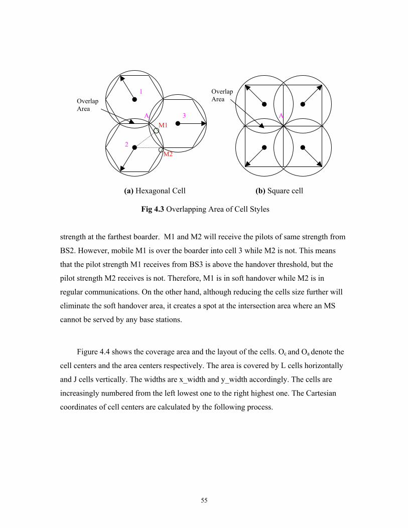
55
(a) Hexagonal Cell (b) Square cell
Fig 4.3 Overlapping Area of Cell Styles
strength at the farthest boarder. M1 and M2 will receive the pilots of same strength from
BS2. However, mobile M1 is over the boarder into cell 3 while M2 is not. This means
that the pilot strength M1 receives from BS3 is above the handover threshold, but the
pilot strength M2 receives is not. Therefore, M1 is in soft handover while M2 is in
regular communications. On the other hand, although reducing the cells size further will
eliminate the soft handover area, it creates a spot at the intersection area where an MS
cannot be served by any base stations.
Figure 4.4 shows the coverage area and the layout of the cells. Oc and Oa denote the
cell centers and the area centers respectively. The area is covered by L cells horizontally
and J cells vertically. The widths are x_width and y_width accordingly. The cells are
increasingly numbered from the left lowest one to the right highest one. The Cartesian
coordinates of cell centers are calculated by the following process.
A
Overlap Area
A
OverlapArea
M1
M2
1
2
3

56
Fig 4.4 Coverage Area and Cell Layout
Assuming that the area center is Oc , the left lowest cell center, the centers of the
cells shall be ),( yx such that
Rjjiy
RlRjjix
123)1(),(
22)1(2)1(),(
×−=
×−+×−= (4.2)
The location of the cell centers can be obtained by moving the origin of the
coordinate system to Oa. i.e. deducting ),( yx with widthx _5.0 and widthy _5.0
respectively.
Toroidal structure is created by seaming up the boarder of the coverage area as
illustrated in Fig 4.5. A mobile , ex. M1, will stay in the area no matter how it moves on
a toroidal structure. In addition, the distance of two locations will change when a planar
area is converted to its toroidal structure as illustrated in Fig 4.5
The creation of a planar cellular coverage area is illustrated in Figure 4.4. We then
convert it into a toroidal circular pipe on o which a mobile cannot move out. Since every
R1
R2
x_width
y_width
L Cells
J Cells x
y
'x
'y
Uncovered Area
Oa
Oc
1 5
3
4
2 6
7
9
8
13
12
11
10
15
14
16
M

57
Fig 4.5 Concept of Toroidal Structure
cell on the circular pipe has the same neighboring situation (6 neighboring hexagonal
cells), a small number of cells are enough to ensure the fidelity of the simulation. We also
do not need to distinguish boarder cells from inner cells.
However, the simple converting scheme shown in Figure 4.5 will fail because that
the actual coverage area is not square as shown in Figure 4.3, and some of the areas can
not be covered. The converting method should seam the somewhat zigzagging boarder of
the actual coverage areas. A new method illustrated by Figure 4.6 is discussed below.
In Figure 4.6 (a), cluster A is the coverage area and cluster B to G are the auxiliary
virtual neighboring clusters used for toroidal adjustment. The centers of the neighboring
cluster can be calculated by the following equations.
0)(22)(
=×=
EyRLEx
15.1)(2)(
RJDyRJDx
×=×=
15.1)(222)(
RJCyRLRJCx
×=×−×=
(4.3)
0)(
22)(=
×−=By
RLBx
15.1)(2)(
RJGyRJGx
×−=×−=
)15.1()(
)222()(RJCy
RLRJCx×−=
×−×−=
Planar Covered Area
B B
Toroidal Covered Area
A
A

58
(a)
(b) (c)
Fig 4.6 Toroidal Adjustment of Mobile Locations and MS to BS Distances
1
2 4
3 5
6
1
2 4
3 5
6
1
2 4
3 5
6
1
2 4
3 5
6
1
2 4
3 5
6
1
2 4
3 5
6
1
2 4
3 5
6
M
a
b
c
a b
c
R1
R2
1 x
y
f(x)
I
IV
II
IIIM2M3
M1

59
Fig 4.7 Mobile Location Adjustment
By toroidal adjustment, mobile M is relocated into cell 6 of the coverage area A
when she moves out off the left boarder of cell 2. The distance from mobile M to base
station 1 is the shortest of the distance a, b, and c. The detail algorithm is discussed
below.
Mobile locations are checked and adjusted periodically. When a mobile moves out
of the coverage area, the toroidal adjustment first determines which neighboring cluster it
moves in and relocates it to the corresponding location in the coverage area. The
relocating algorithm is illustrated below where Ω represents the neighboring cluster sets
consisting of B-G.
The judgment of whether mobile M is in a certain cluster is made by the following
steps illustrated by Figure 4.6 (c).
1. find the nearest cell center in the cluster to the mobile M
2. mapping the location of M into the first quadrant of that cell
3. M is in the cluster if ))(()( MxfMy < , otherwise not
M in Coverage Area A ?
New M Location
)),(min(such that ,
HMdistH Ω∈ M in Cluster
H?
y(M)y(M)_newx(M)x(M)_new
==
Seclude H from Ω
y(H)-y(M)y(M)_newx(H)-x(M)x(M)_new
==
T
F T
F
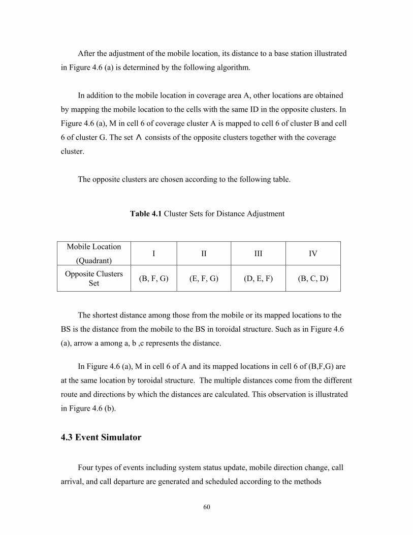
60
After the adjustment of the mobile location, its distance to a base station illustrated
in Figure 4.6 (a) is determined by the following algorithm.
In addition to the mobile location in coverage area A, other locations are obtained
by mapping the mobile location to the cells with the same ID in the opposite clusters. In
Figure 4.6 (a), M in cell 6 of coverage cluster A is mapped to cell 6 of cluster B and cell
6 of cluster G. The set Λ consists of the opposite clusters together with the coverage
cluster.
The opposite clusters are chosen according to the following table.
Table 4.1 Cluster Sets for Distance Adjustment
Mobile Location
(Quadrant) I II III IV
Opposite Clusters Set (B, F, G) (E, F, G) (D, E, F) (B, C, D)
The shortest distance among those from the mobile or its mapped locations to the
BS is the distance from the mobile to the BS in toroidal structure. Such as in Figure 4.6
(a), arrow a among a, b ,c represents the distance.
In Figure 4.6 (a), M in cell 6 of A and its mapped locations in cell 6 of (B,F,G) are
at the same location by toroidal structure. The multiple distances come from the different
route and directions by which the distances are calculated. This observation is illustrated
in Figure 4.6 (b).
4.3 Event Simulator
Four types of events including system status update, mobile direction change, call
arrival, and call departure are generated and scheduled according to the methods

61
proposed in [39]. An event simulator consists of an events generator, an events scheduler
and an events handler as shown in Figure 4.2.
Fig 4.8 Events Generating and Scheduling
Event generator generates the events. The call arrivals are assumed following
Poisson processes and the call departures have their service time exponentially
distributed. The inter-arrival time τ of the new calls follow the exponential distribution as
λτλτ −= epT )( (4.4)
where λ is the mean arrival rate. The service time s (call duration) also follow the
exponentially distributed as s
S esp µµ −=)( (4.5)
where µ is the mean call departure rate. The average service time is µ/1=H .
The processing of the call arrivals and departures by the system can be view as a
M/M/m/m queue which has poison arrival (Markov), exponential departure times
(Markov), m servers and the system capacity supporting m customers. Assuming block
call clear, memoriless arrivals and infinite users, the theoretical blocking probability is
given by Erlang B formula [40] as
Call Arrival Generator
Call Depart Generator
System Update Events Generator Event
Handler
updateupdateupdate
Call Depart
Call arrivalCall Arrival
Time

62
∑=
= C
k
k
C
B
kA
CAP
0!
! (4.6)
where HA λ= is the offered traffic measured in Erlang and C is the number of available
channels.
System status update is performed at a fixed rate. After every time interval sT , the
mobile statuses are updated and handovers are checked.
The events scheduler saves into a waiting list the type of a new event and its time
stamp set as its arriving time. It picks up from the waiting list an event A with the
smallest time stamps for processing. After calling the event handler, it deducts the time
stamp AT from the time stamps of all the events in the waiting list. Any event with a non-
positive time stamp will be dropped from the waiting list.
Events handler will call the functions such as call arrival, call departure or system
update according to the type of the events. Call arrival function will find the candidate
serving BS and run CAC. Call departure function will delete the information of the
departing mobile from certain status tracking lists. System update function will update
the mobile locations and check possible handovers.
4.4 Channel Simulator
The channel simulator generates multipath profiles and the corresponding Rayleigh
fading curves. The multipath profiles are assumed uniform over the coverage area. Each
multipath component between a MS and a BS has a unique fading curve.
WCDMA systems adopt a chip rate as 3.84Mcps and are wideband systems where
all the multipath components are resolvable. The method from [41] is used to generate
multipath profiles. Vehicular outdoor channel profile is used to characterize the channel

63
model. The mobile speed is assumed to be 120 miles per hour and the corresponding
Doppler spreads is 213 Hz. The power delay profile (PDF) is shown in Table 4.2.
Table 4.2 Vehicular Outdoor Channel PDF
The continuous time based PDF is then converted to the discrete PDF using ray
splitting method below.
Each multipath component (ray) is split into two rays at the adjacent sampling point
by the following rule. The sum of the power of the split components is equal to that of the
original component. The power of each split component is inversely proportional to its
distance to the original component. If there are more than two split components at the
same sampling point, they are added together as one discrete multipath component. All
the discrete multipath components are normalized such that the channel does not change
the signal energy.
One independent Rayleigh waveforms is generated for each multipath components
using Clarks model [40]. A Doppler filter is created according to the Doppler spreads.
Two complex Gaussian random variables are generated independently in frequency
domain and passed through the Doppler filter which correlates the samples. The filtered
samples are converted into time domain by inverse fast Fourier transformation (IFFT).
The real parts of the outputs are used respectively as the real and imaginary parts of the
Rayleigh fading coefficients. The complex curve has amplitudes following Rayleigh
distribution and phases uniformly distributed between 0 and π2 .
-20
2510
-15
1730
-10
1090
-9
710
-1
310
0
0
Avg. Power
Delay (ns)

64
Fading data should be continuous across the frames or slots. A large volume of
fading data is generated so that the fading curves are continuous over a long period of
time. Then, the curve is reused from the start. Interpolating and zero-order holding are
used to generate interval sampling points of the fading data. A large number of fading
curves are generated and stored. One fading curve is assigned to one multipath
components of each existing link from a MS to a BS. Each time a new call arrives, free
fading curves by the number of multipath components times the number of BS are
selected from the pool and assigned to that MS.
Each channel from a MS to a BS is a linear time varying filter as in Figure 4.9
where iZ τ− denotes the delay of iτ samples, ic represents the strength of the multipath
component and ir is the Rayleigh waveform. White Gaussian noise is added at the
receiver. The noise power is calibrated by the following process.
The carrier to noise power ratio is
WNRE
NC bb
××
=0
(4.7)
where WRNC b ,,, are signal power, noise power, bit rate, and chip rate respectively.
Therefore, the noise power can be obtained as
1C when 0
0
0
0
0
0
0
==
×=×=
NE
S
NE
SCNE
RWCN
f
f
(4.8)

65
Fig 4.9 Time Varying Channel
4.5 Signal Processor
The signal processor includes a transmitter and a receiver. WCDMA physical layer
structure is described in [43]. The up-link transmitting and receiving schemes are
discussed below.
WCDMA up-link dedicated physical channels (DPCH) include several dedicated
physical data channels (DPDCH) and one or none dedicated physical control channel
(DPCCH). Spreading is applied to the physical channels in two steps. Channelization
spreads the data in each channel with Orthogonal Variable Spreading Factor (OVSF)
code with a gain factor. The spread DPDCH data are transmitted in I or Q channels and
DPCCH data is transmitted only in Q channel. Scrambling code for UE identification are
then multiplied to the complex data. The scrambled data is modulated as QPSK signals
with real part into I channel and imaginary part into Q channel. The spreading and
modulation processes are illustrated in Figure. 4.7. In simulation model, one DPDCH
channel with no DPCCH is simulated for each user with the gain factor 1=dβ .
Rectangular pulse shaping is used instead of standardized raise cosine filter with rolloff
factor as 0.22.
Transmitted Signals
11 rc ×
2τ−Z
22 rc ×
NN rc ×
NZ τ−
Multipath 1
Multipath 2
Multipath N
M M
Received Signals
Noise

66
The channelization codes are generated according to the following rule.
10,1, =chC (4.9)
=
=
1 111
-
0,1,0,1,
0,1,0,1,
1,2,
0,2,
-
CCCC
CC
chch
chch
ch
ch (4.10)
=
−−
−−
++
++
+
+
+
+
−
−
-
-
-
11
11
11
11
1
1
1
1
2,2,2,2,
2,2,2,2,
1,2,1,2,
1,2,1,2,
0,2,0,2,
0,2,0,2,
12,2,
22,2,
3,2,
2,2,
1,2,
0,2,
nnnn
nnnn
nn
nn
nn
nn
nn
nn
n
n
n
n
chch
chch
chch
chch
chch
chch
ch
ch
ch
ch
ch
ch
CC
CC
CC
CC
CC
CC
C
C
C
C
C
C
MM
(4.11)
jichC ,, refers to the j th channel code with spreading factor (SF) as i . OVSF code
preservers the orthogonality between the signals in any two physical channels of a user.
Codes are selected in the following steps.
1. The DPDCH channel is always spread by 0,256,chc CC =
2. When only one DPDCH exist, it is spread by kSFchd CC ,,1, = where SF is the
spreading factor and 4/SFk = .
3. For multiple DPDCH, all DPDCH have the spreading factor
4=SF , kchnd CC ,4,, = where 1=k if )2,1(∈n , 2=k if )6,5(∈n , and 3=k if
)4,3(∈n

67
Fig 4.10 WCDMA Physical Channel Spreading and Modulation
The long scrambling sequences nlongc ,1, and nlongc ,2, are constructed from the
modulo 2 sum of two binary m-sequences generated from two generator polynomials of
degree 25. Let x and y be the two m-sequences respectively. The x sequence is
constructed using the primitive polynomial 1325 ++ XX . The y sequence is constructed
using the polynomial 12325 ++++ XXXX . The resulting sequences thus constitute
the segments of a Gold sequences set. Sequence nlongc ,2, is a 16777232 chip shifted
version of sequence nlongc ,1, . Scrambling code generation is discussed in detail as
follows.
1DPDCH 1,dC dβ
3DPDCH 1,dC dβ∑
Pulse Shaping
Pulse Shaping
5DPDCH 1,dC dβ
2DPDCH 1,dC dβ
4DPDCH 1,dC dβ
∑6DPDCH 1,dC dβ
I
Q
j
ndpchS ,
S
Re(S)
Im(S)
)cos( tω
)sin( tω−
DPCCH 1,dC dβ
Codeion Channeliza , , cid CC Code ScramblingComplex ,ndpchS factorgain , cd ββ

68
Let 023 nn L be the 24 bit binary representation of the scrambling sequence number
n with 0n denoting the least significant bit. The x sequence is denoted as nx and depends
on the scrambling sequence number n . Next, let )(),( iyixn denote the i th symbol of the
sequence nx and y respectively. The m-sequences nx and y are constructed as follows.
Set initial conditions as
1)24()23()1()0(1)24(,)23(,)1(,)0( 2310
========
yyyyxnxnxnx nnnn
L
L (4.12)
Recursively define subsequent symbols:
272,,0,2 modulo )()3()25( 25 −=++=+ Kiixixix nnn (4.13)
272,,0,2 modulo )()1()2()3()25( 25 −=++++++=+ Kiiyiyiyiyiy (4.14)
Define the binary Gold sequence nz by:
22,,0,2 modulo )()()( 25 −=+= Kiiyixiz nn (4.15)
Next, the real value Gold sequence nZ can be defined as
22,1,0for 1)( if 10)( if 1
)( 25 −=
=−=+
= Kiiziz
iZn
nn (4.16)
The real-value long scrambling sequences nlongc ,1, and nlongc ,2, are defined as follows.
22,1,0 )),1(2 modulo )16777232(()(
22,1,0 ),()(2525
,1,
25,1,
−=−+=
−==
K
K
iiZic
iiZic
nnlong
nnlong (4.17)

69
The complex value long scrambling sequence nlongC , , is defined as:
))2/2()1(1)(()( ,2,,1,, icjiciC nlongi
nlongnlong −+= (4.18)
where 22,1,0 25 −= Ki and denotes rounding to the nearest lower integer.
RAKE Receiver and Maximum Ratio Combining (MRC) are used at the BS. The
number of fingers is four. Assuming that the channels are perfectly estimated, both the
phase distortion and the delay are known. The received signals are first realigned and
phase compensated. Then, the signals are resampled, descrambled and despread before
the MRC is used to generate the hard decisions. The Receiving process is illustrated
below.
Fig 4.11 Receiver Structure
Received Signal
Finger 1
Finger 2
Finger K
Phase CompensationRealignment Resampling
Phase CompensationRealignment Resampling
Phase CompensationRealignment Resampling
M
ndpchS , idC ,
ndpchS , idC ,
ndpchS , idC ,
MRC

70
4.6 Smart Antenna Processing
Switched-beam and adaptive beamforming are used. The smart antenna processing
are illustrated in Figure 4.9 below.
When signal 1S , 2S , , NS arrive, the antenna output 1R , 2R , , NR are generated
according to the AoA θ . Switched beam beamformer multiplies the array output with the
weight vectors, and chooses the weight vector which produces the maximum combining
output to be the desired combining weight vector. Adaptive steering uses the array
response as the desired weights. The array outputs are multiplied with the Hermitian of
the combining weights in the combining process. The outputs of the combiner then go to
the WCDMA receiver.
Fig 4.12 Smart Antenna Processing
Combining
Weight Update
Channel CompensatingDespreading Rake Receiving
1R
NR
2R
Switched
Adaptive Steering
2R
NR
1R
iS
cW
Decision
1W
2W
NW
ic WW =
maximize output
1S
NS
1S
NS
M
M
1S
NSM
iθ )sin()1( θπ ×−××= mjeW

71
4.7 Resource Management
We use power control based on constant power level in the simulator. The received
power levels of every cell are the same. SINR are not balanced in this case since the
interference varies in each cell. However, the interference level does not differ much
since the mobiles tend to be uniformly distributed. The SINR balancing will improve the
performance a little, but does not affect the simulation study much.
The TPC for power control has two bits instead of one in WCDMA proposal, but
provide a more adaptive scheme to mitigate severe Doppler fade.
In order to simplify the simulation, power control commands are given by one BS in
the active set identified as a controlling BS such that a single TPC command is received
in each slot.
Pilot signals from different multipathe components are combined by MRC to
generate a single estimation of the pilot strength. Angular diversity (through beam
forming) is expected to smooth the fading effect and reduce power control errors.
However, this expectation can not be met as shown in the simulation results in next
chapter.
Handover is simulated based on IS-95 standard. Only the active set is simulated in
order to cut down the complexity. An incoming call is added to active set if all the
following condition satisfied.
. The pilot strength goes above T_ADD.
. The active set is not full.
. CAC gives permission.
Whenever the pilot strength drops below T_DROP, the BS is dropped from the active set
without waiting for the timer to expire.

72
Call admission control and channel reservation are based on constant power level
based PC scheme. Assuming that the received powers in every cell are the same,
Equation (3.6), (3.7) become
>Ω∈=
=otherwise ,0
;0)( if ),(or |)(min jRkjkjjRR (4.19)
where
Ω∈−−
=−=
);( if ,),(
; if , )(
kjkhLII
kjIIjR
mkTH
kTH (4.20)
THI is the total interference and noise threshold, and kI is the current interference in the
k th cell.
Because of unbalanced SINR and constant signal power, HIM in section 3.4 is
replaced by a handover interference threshold THHI . The total interference margin is
renamed as total interference threshold THTI . The current interference margin CIM is
replaced by the current interference CI . Therefore, The CAC and Channel Reservation
can be illustrated as Figure 4.13 below.
Fig 4.13 CAC and Channel Reservation Scheme
Read Interference level CI
THHICI >
Handover ?
Admit the request
Reject the request
Yes No
NoYes
Yes
No THTICI >

73
Chapter 5
Simulation Result and Discussions
This chapter discusses the simulation experiments and the results generated by the
model described in Chapter four. The performances considered include bit error rate,
power control rate, power control errors, handoff rate, call blocking rate and handoff
failure rate, etc. Only the uplink scenario is considered in the following simulation
experiments.
5.1 General Description of the Simulation Setup
Unless specified, simulation experiments follow the general setup described in this
section. The Doppler frequency is 213 Hz. Power control rate is one command per slot
(1500 Hz). The power control parameters are set as
pc_step = 0.5dB basic unit of increment or decrement
incre_step = 3.2 multiplicity of increment (number of
pc_step)
decre_step = 3.2 multiplicity of decrement (number of
pc_step)
sig_target = 0dB target signal power at the receiver
sig_th_low = -8dB lower threshold for incre_step;
sig_th_high = 8dB higher threshed for decre_step;
pwr_ms_max = 1.5 / t_drop maximum MS power
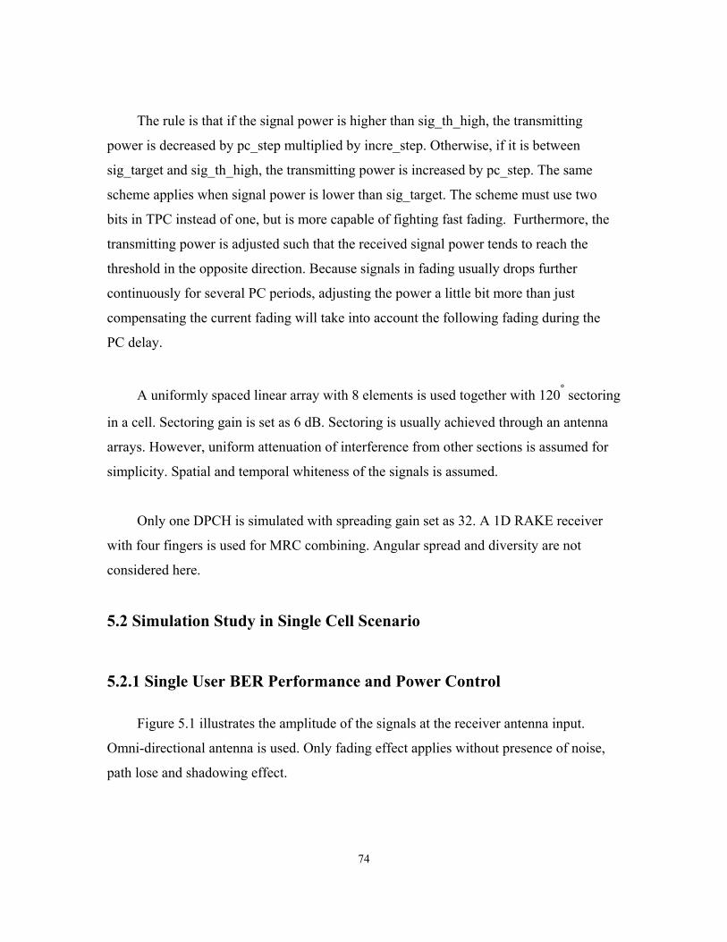
74
The rule is that if the signal power is higher than sig_th_high, the transmitting
power is decreased by pc_step multiplied by incre_step. Otherwise, if it is between
sig_target and sig_th_high, the transmitting power is increased by pc_step. The same
scheme applies when signal power is lower than sig_target. The scheme must use two
bits in TPC instead of one, but is more capable of fighting fast fading. Furthermore, the
transmitting power is adjusted such that the received signal power tends to reach the
threshold in the opposite direction. Because signals in fading usually drops further
continuously for several PC periods, adjusting the power a little bit more than just
compensating the current fading will take into account the following fading during the
PC delay.
A uniformly spaced linear array with 8 elements is used together with 120° sectoring
in a cell. Sectoring gain is set as 6 dB. Sectoring is usually achieved through an antenna
arrays. However, uniform attenuation of interference from other sections is assumed for
simplicity. Spatial and temporal whiteness of the signals is assumed.
Only one DPCH is simulated with spreading gain set as 32. A 1D RAKE receiver
with four fingers is used for MRC combining. Angular spread and diversity are not
considered here.
5.2 Simulation Study in Single Cell Scenario
5.2.1 Single User BER Performance and Power Control
Figure 5.1 illustrates the amplitude of the signals at the receiver antenna input.
Omni-directional antenna is used. Only fading effect applies without presence of noise,
path lose and shadowing effect.

75
Figure 5.1 shows that because of the fading effect, signals are widely fluctuating.
Fast power control mitigates the fading effect, but still can not catch up with the change
of the channel when sharp and fast fading happens. Therefore, high pikes and deep abyss
still exist along the curve with power control. The curve after power control is more
likely to be smooth in slow fading circumstances.
Fig 5.1 Received Signal at BS
Figure 5.2 illustrates the fading curves with different Doppler frequencies. As
shown in the graph, fading channel with lower Doppler spreads changes more slowly and
smoothly while that with higher Doppler spreads changes fast and sharply. It is easier to
combat slow fading than fast fading by power control.

76
Fig 5.2 Fading Curves with Different Doppler Spreads
Figure 5.3 shows the link performance (BER) at the output of the receiver with fast
power control applied to the system. The power control parameters are adjusted
according to different fading situations. The parameters used for 213 Hz (Doppler
spreads) are described before in Section 5.1. Parameters for 10 Hz and 100 Hz are as
follows.
For 10 Hz, pc_step = 0.1dB; incre_step = 2; decre_step = 2; sig_target = 0dB;
sig_th_low = -0.1dB; sig_th_high =0.1dB.
For 100 Hz, pc_step = 0.3dB; incre_step = 2; decre_step = 2; sig_target = 0dB;
sig_th_low = -0.3dB; sig_th_high = 0.3 dB.

77
Fig 5.3 BER with PC under Different Doppler Spread
Result with theoretically perfect power control is derived using optimistic
estimation of the BER in CDMA system considering the multipath effect.
−×=N
KE
NQPb
e 21
21 0 (5.1)
where K refers to the number of the multipath components, and N is the spreading gain.
The powers of the multipath components are assumed to be equal after power control.
Figure 5.3 illustrates that bit error rate increases with higher Doppler spreads. Power
control can mitigate the fading effect, especially in slow fading.

78
Figure 5.4 shows the power control error with respect to fading of different Doppler
spreads and different diversity schemes. Consistent to figure 5.3, power control errors
increase with the increase of the Doppler spreads.
Fig 5.4 Power Control Error with Respect to Doppler Spreads
and Diversity Schemes.
Power control schemes without exploring the diversity estimate the pilot strengths
directly. Power control schemes exploring the diversity assume that multipath
components are resolved perfectly by the smart antenna. The signal strengths of
multipath components are combined according to the Maximum Ratio Combine (MRC)
scheme into a single estimation of the signal power. Power control command is
calculated based on this estimation.

79
It can be seen from Figure 5.4 that the PC errors (standard deviation) of the
estimated pilot and the PC errors of the signal with diversity do not differ much from the
PC errors of the signal without diversity.
Figure 5.5 further shows that the bit error rate does not improve by employing the
diversity scheme in power control.
Fig 5.5 BER with Respect to Doppler Spreads
and Diversity Schemes
Figure 5.6 illustrates how shadowing affects the performance. Slow power control
compensates only the path loss and the shadowing effect. As shown in the figure,
shadowing effect degrades the performance by a small amount when either fast PC or
slow PC is applied.
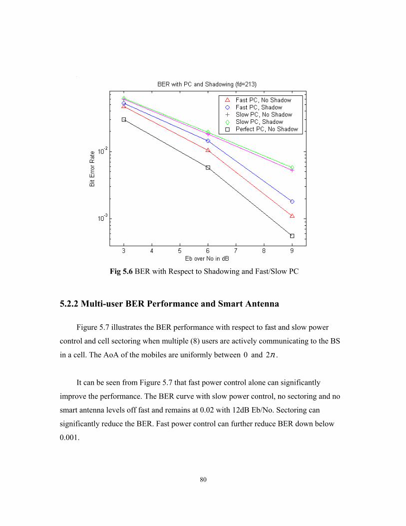
80
Fig 5.6 BER with Respect to Shadowing and Fast/Slow PC
5.2.2 Multi-user BER Performance and Smart Antenna
Figure 5.7 illustrates the BER performance with respect to fast and slow power
control and cell sectoring when multiple (8) users are actively communicating to the BS
in a cell. The AoA of the mobiles are uniformly between 0 and π2 .
It can be seen from Figure 5.7 that fast power control alone can significantly
improve the performance. The BER curve with slow power control, no sectoring and no
smart antenna levels off fast and remains at 0.02 with 12dB Eb/No. Sectoring can
significantly reduce the BER. Fast power control can further reduce BER down below
0.001.
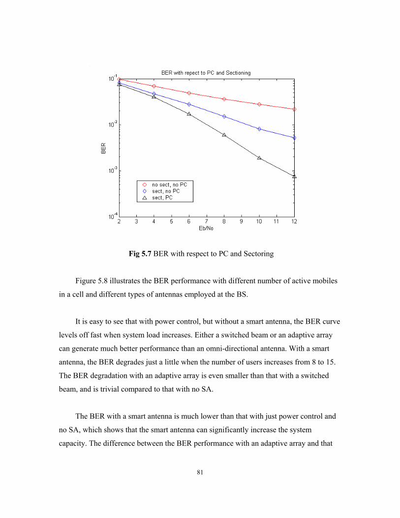
81
Fig 5.7 BER with respect to PC and Sectoring
Figure 5.8 illustrates the BER performance with different number of active mobiles
in a cell and different types of antennas employed at the BS.
It is easy to see that with power control, but without a smart antenna, the BER curve
levels off fast when system load increases. Either a switched beam or an adaptive array
can generate much better performance than an omni-directional antenna. With a smart
antenna, the BER degrades just a little when the number of users increases from 8 to 15.
The BER degradation with an adaptive array is even smaller than that with a switched
beam, and is trivial compared to that with no SA.
The BER with a smart antenna is much lower than that with just power control and
no SA, which shows that the smart antenna can significantly increase the system
capacity. The difference between the BER performance with an adaptive array and that

82
Fig 5.8 BER with respect to SA and Number of Users
with a switched beam increases when the system load goes up. However, it is still small
compared to the overall performance.
Figure 5.9 shows the BER as a function of the number of users with Eb/No equal to
12dB. Similarly, the adaptive arrive and the switched beam generate comparable
performances, but much better than that with omni-directional antennas. Figure 5.9 also
shows that the BER levels off when system load approaches a high level. However, the
BER with a smart antenna remains very low even with a large number of users. Thus, the
system capacity is tremendously increased.

83
Fig 5.9 BER with respect to SA and No. of Users
Figure 5.10 illustrates the tradeoff of SA for lower PC rate. Eight users in a cell and
the BS with an adaptive array are assumed in the experiment. The half rate PC (750 Hz)
is similar to that in IS-95 (800 Hz).
We can see from Figure 5.10 that half rate PC without SA generates performance
noticeably worse than that of slow PC with SA. This means that SA is better than fast PC
in improving the performance. Also noticeable is that slow PC with SA and half rate PC
with SA have similar performance compared to that of fast PC without SA. This shows
that performance improvement by SA can be traded for the reduction of the PC rate.
However, fast PC with SA gives much better performance than all other cases, showing
the benefit of using SA in WCDMA systems.

84
Fig 5.10 BER with respect to PC Rate and SA
5.2.3 Cell Capacity, Block/Drop Rate and Smart Antenna
Table 5.1 below shows the number of users with respect to the ratio of arrival and
departure rate. The call admission and drop thresholds are set up as infinity. The
measurements are the total interference and noise power level at the BS.
Arrival/Departure Ratio 2 6 10 14 18 22
Number of Users In the Cell
2.6 6.65 9.98 13.44 17.43 21.34
Table 5.1 Number of Users with respect to Arrival/Departure Ratio
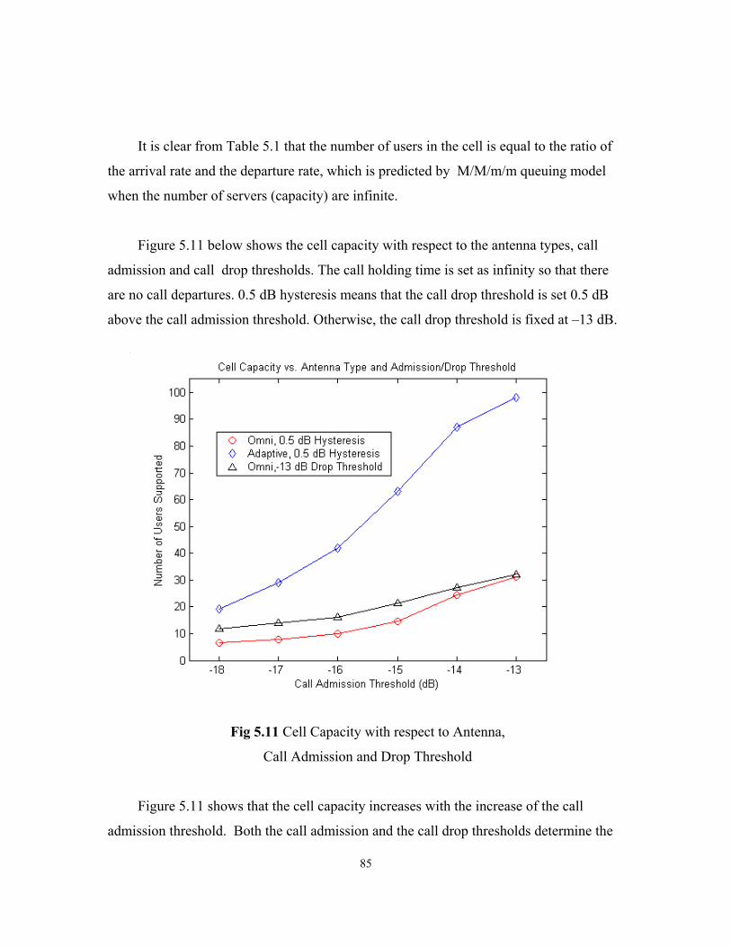
85
It is clear from Table 5.1 that the number of users in the cell is equal to the ratio of
the arrival rate and the departure rate, which is predicted by M/M/m/m queuing model
when the number of servers (capacity) are infinite.
Figure 5.11 below shows the cell capacity with respect to the antenna types, call
admission and call drop thresholds. The call holding time is set as infinity so that there
are no call departures. 0.5 dB hysteresis means that the call drop threshold is set 0.5 dB
above the call admission threshold. Otherwise, the call drop threshold is fixed at 13 dB.
Fig 5.11 Cell Capacity with respect to Antenna,
Call Admission and Drop Threshold
Figure 5.11 shows that the cell capacity increases with the increase of the call
admission threshold. Both the call admission and the call drop thresholds determine the

86
capacity of the cell. However, the major factor determining the capacity is the call
admission threshold since it is below the call drop threshold. Larger hysteresis will
increase the capacity, but just a little. On the other hand, smart antenna obviously
increases the system capacity.
Figure 5.12 shows the number of users in a cell of finite capacity with call
admission thresholds as 17 dB and call drop threshold as 16 dB. The estimated
capacities are 10 users with an omni-directional antenna and 29 users with an adaptive
array.
Fig 5.12 Number of Users with Finite Cell Capacity
It can be seen from the figure that with SA, there are many more users in the cell
when the ratio of arrival rate over departure rate is large. For omni-directional antenna,
there are just about 8 users remaining in the cell even if the ratio reaches 20, showing that
the majority of the new call requests were rejected.
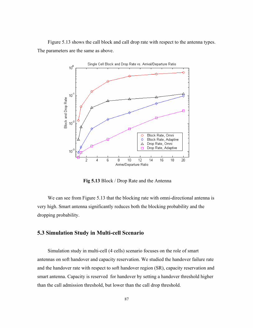
87
Figure 5.13 shows the call block and call drop rate with respect to the antenna types.
The parameters are the same as above.
Fig 5.13 Block / Drop Rate and the Antenna
We can see from Figure 5.13 that the blocking rate with omni-directional antenna is
very high. Smart antenna significantly reduces both the blocking probability and the
dropping probability.
5.3 Simulation Study in Multi-cell Scenario
Simulation study in multi-cell (4 cells) scenario focuses on the role of smart
antennas on soft handover and capacity reservation. We studied the handover failure rate
and the handover rate with respect to soft handover region (SR), capacity reservation and
smart antenna. Capacity is reserved for handover by setting a handover threshold higher
than the call admission threshold, but lower than the call drop threshold.

88
Figure 5.14 shows the call drop rate with respect to antenna types and the capacity
reservation. Parameters are as described in the next two paragraphs, and remain the same
in the following experiments unless specified.
For omni-directional antennas, the small SR refers to adding the call to the
candidate set if the mobile moves into 1/20 of the cell radius beyond the boarder, and
dropping the call when it moves beyond 1/10 of the cell radius from the boarder. For
large SR, the parameters are 1/8 when adding and 1/4 when dropping. For adaptive
arrays, the small SR refers to 1/100 when adding and 1/200 when dropping, while large
SR refers to 1/20 when adding and 1/10 when dropping.
Fig 5.14 Call Drop Rate with respect to Antenna Types, SR, and Reservation
Large reservation refers to -19dB for denying admissions, -18 dB for blocking
handovers and 16.5 dB for dropping ongoing calls. Small reservation refers to -18.2 dB

89
for denying admissions, -18 dB for blocking handovers and 16.5 dB for dropping
ongoing calls.
From figure 5.14, we can see that the call drop rates do not differ much with respect
to SR. The call drop rates go up considerably when the reservation is small. However,
they can be driven back by smart antennas. The call drop rates with omni-directional
antennas and large reservation are even higher than that with smart antennas, but small
reservation. The call drop rates with smart antennas and large reservation are the lowest
among all, but just a little bit lower than that with smart antenna and smaller reservation.
Figure 5.15 shows the handover rates with respect to antenna types and SR. The
reservation is set as large, but is not relevant to the handover rate. From the figure, the
handover rate is solely a function of SR.
Fig 5.15 Handover Rate with respect to Antenna Type and SR

90
Figure 5.16 below shows the handover failure rates with respect to antenna types
and SR. The reservation is set as large. It is easy to see that the reduction of handover
failure rate by SR is very small. The reduction by smart antenna, on the other hand is
significant. SR is mainly for seamlessly handover the call. Enlarging SR can reduce the
handover failure rate a little bit just because a handover call can wait longer for the cell
regaining its capacity before blocking the handover. The major factor affecting SR is the
time period required to guarantee a seamless handover. Smart antennas have little to do in
reducing the SR and corresponding soft handover rate.
Fig 5.16 Handover Failure Rate with respect to Antenna and SR
Figure 5.17 shows the call block rates with respect to antenna types and SR. The
reservation is set as large. Again, it is easy to see that SR has little influence on the call
block rates whereas smart antennas reduce the call block rates significantly.
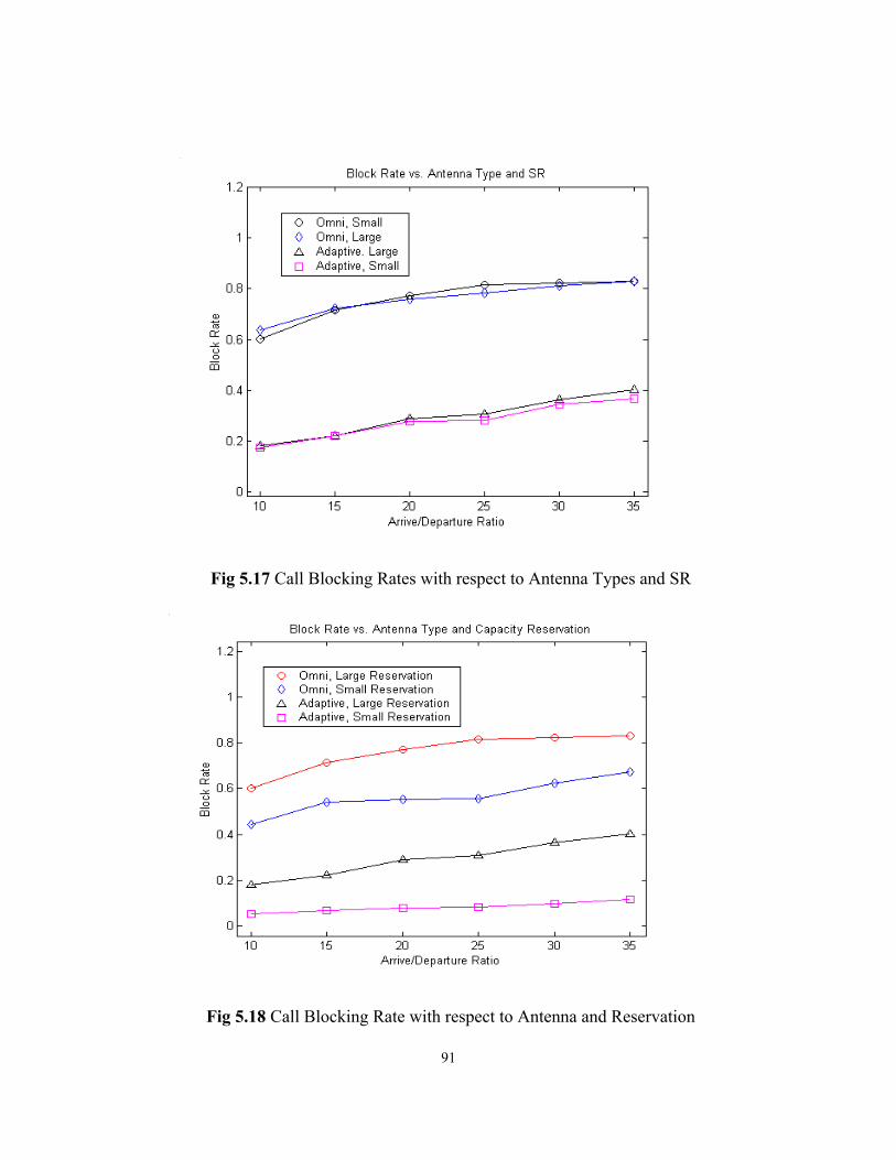
91
Fig 5.17 Call Blocking Rates with respect to Antenna Types and SR
Fig 5.18 Call Blocking Rate with respect to Antenna and Reservation

92
Figure 5.18 shows the call blocking rates with respect to antenna types and
reservation. Either reducing the capacity reservation or employing smart antennas
reduces the call blocking probability considerably. Using smart antenna, among the two,
is more effective in reducing the call blocking rates.
Fig 5.19 Handover Failure Rate with respect to Antenna and Reservation
Figure 5.19 shows the handover failure rates with respect to antenna types and
reservation. It can be seen that contrary to the blocking rates in Figure 5.18, handover
failure rates with small reservation is much higher than that with large reservation and
omni-directional antenna. However, with smart antenna, the increase of the handover
failure rates is very small when we change from large reservation to small reservation.
Smart antenna can maintain the handover failure rates as if the reservation is not reduced.
The reservation reduced can be used to accommodate more calls and the system capacity
is increased, shown as the big reduction in the call block rates in Figure 5.18.
93
Chapter 6
Conclusion and Future Work
Although optional in 3G proposals, deploying smart antenna can significantly
increase the capacity of the radio networks. In this thesis, we compare several aspects of
different smart antenna algorithms including switched beam and adaptive arrays. A multi-
cell simulation model is built which consists of six integrated components including a
mobility and geographic model, an event simulator, a channel simulator, a WCDMA
signal processor, a smart antenna processor and a resource management model. We also
pursue simulation studies, investigating the benefit from smart antenna techniques to both
the bit error rate (BER) performance improvement and the enhancement to the radio
resource management schemes.
6.1 Conclusions
Adaptive arrays and switched beam antennas are two smart antenna (SA)
approaches providing significant interference reductions in future cellular systems. Both
algorithms have similar requirements on hardware. The computational complexity
depends on individual algorithms. Algorithms such as CGA and MPL are designed to
take advantage of the CDMA signal structures, and are more suitable than switched beam
antennas when applied to CDMA systems with large number of users.
Both adaptive arrays and switched beam antennas generate comparable
performances if the interference and noise signals are spatially and temporally white.
Fully adaptive algorithms can produce much better performances than that of switched

94
beam if whiteness does not hold and the number of users is less than the number of array
elements. However, they will fail when there are more users than array elements. Sub-
optimal adaptive algorithms such as sub-optimal CGA and MPL are most likely the
suitable algorithms for practical cellular systems due to their good performances,
robustness, and low complexity.
Smart antenna techniques can significantly enhance the performances and capacity
of the CDMA radio networks. With eight array elements, the capacity could be increased
by a factor of 4. With moderate number of users, the BER will be improved by nearly
102 . Smart antennas also help to enhance the capability of radio resource management.
The mobile transmitting power could be lower because of the interference reduction.
Although the power control errors cannot be reduced by exploring the angular diversity
provided by beamforming, the power control command rates can be reduced through the
tradeoff with the interference reduction by smart antennas. On the second hand, smart
antennas will significantly increase the system capacity and reduce the call blocking
rates. Smart antennas also obviously reduce the handover failure rates. Therefore, the
system capacity can be increased further by reducing the resources reserved for soft
handover without increasing the handover failure rates. However, smart antenna does not
play a big role in reducing soft handover rates. Handover rates can be reduced by
decreasing SR, which generally does not obviously increase handover failure rates.
6.2 Future Works
Immediate follow up studies could be pursued in investigating smart antenna effect
on performances and resource management in heterogeneous cell environments where a
cell with an omni-directional antenna could suffer from his neighboring BS employing a
smart antenna. The experiment can be done by setting the predefined parameter
bs_type the proper value in the pre-processor. Another follow up is to study the issues
with different traffic patterns, which may require a traffic pattern generator.
95
The simulator is open, and capable of integrating or replacing the original modules
with new modules. New modules could include other smart antenna algorithms and
resource management schemes, AoA spread models, 2-D rake receivers, sidelobe
reduction algorithms, other propagation and channel modules. Some of the models have
been introduced in Chapter two and three, such as SINR balanced power control
algorithms, and statistics assisted handover, etc.
Another direction is to adopt the simulator as a platform in studying the network
layer issues such as the end to end performance analysis and investigation in QoS,
especially with multi-rate traffic (voice and data). Progress in this direction may require a
multi-rate spreading/despreading schemes and channel coding. QoS schemes such as
channel reservation and queuing could also be investigated. Queuing problems could be
investigated by replacing call block clearing with specific queuing modules in the
simulator.

96
Reference
[1] Harri Holma, Antti Toskala, WCDMA for UMTS (Radio Access for Third Generation
Mobile Communications), John Willy & Sons Ltd, West Sussex, England, 2001.
[2] Theodore S. Rappapport, Wireless Communications (Principles and Practice),
Prentice Hall PTR, New Jersey, 1996.
[3] Jerry D. Gibson, The Mobile Communications Handbook, CRC Press, 1996.
[4] M. Zeng, A. Annamalai, Vijay K. Bhargava, Recent Advances in Cellular Wireless
Communications, IEEE Communication Magazine, pp. 128-138, September, 1999.
[5] Francis Swarts, Pieter Van Rooyan, Ian Oppermann, Michiel P. Lotter, CDMA
Techniques for Third Generation Mobile Systems, Kluwer Academic Publishers,
Massachusetts, 1999.
[6] John Litva, Titus Kwok-Yeung Lo, Digital Beamforming in Wireless
Communications, Artech House, Boston, 1996.
[7] Adrian O. Boukalov, Sven-Gustav Haggman, System Aspect of Smart-Antenna
Technology in Cellular Wireless Communications-An Overview, IEEE Transactions on
Microwave Theory and Techniques, vol. 48, no. 6, pp. 919-929, June 2000.
[8] S. Anderson, U. Forssen, J. Karlsson, T. Witzschel, P. Fisher, and A.Krug, Ericsson
/Mannesmann GSM Field-trials with Adaptive Antennas, Proc. IEEE 47th VTC, pp.
15871591, 1997.

97
[9] S. Anderson, Adaptive Antennas for GSM, presented at the 5th Stanford Smart
Antennas Mobile Wireless Communication Workshop, July 2324, 1998.
[10] K. Molnar, Spacetime Processing in The Evolution of IS-136 System, presented
at the 5th Stanford Smart Antennas Mobile Wireless Communication Workshop, July 23
24, 1998.
[11] B. Hagerman, T. Osterman, K. J. Molnar, and G. E. Bottomly, Field Test
Performance Results for D-AMPS in PCS Bands with Array Processing, Proc. IEEE
VTC97, Phoenix, AZ, pp. 15821586, 1997.
[12] J. H. Winters, Forward Link Smart Antennas and Power Control for IS-136,
presented at the 5th Stanford Smart Antennas Mobile Wireless Communications
Workshop, July 2324, 1998.
[13] R. L. Cupo, G. Golden, C. Martin, and J. H. Winters, A Four-element Adaptive
Antenna Array for IS-136 PCS Base Stations, in Proc. IEEE VTC97, Phoenix, AZ, pp.
15771581, 1997.
[14] F. Adachi, Application of Adaptive Antenna Arrays to W-CDMA Mobile Radio,
presented at the 5th Stanford Smart Antennas Mobile Wireless Communications
Workshop, July 2324, 1998.
[15] G. Tsulos, M. Beach, and J. McGeen, Wireless Personal Communications for The
21st Century: European Technology Advances in Adaptive Antennas, IEEE
Communication Magazine, pp. 102109, Sept. 1997.

98
[16] J. Monot, J. Thibault, P. Chevalier, F. Pippon, and S. Mayrague, Smart Antenna
Prototype for the SDMA Experimentation in UMTS and GSM/DCS1800 Network, in
IEEE PIMCR97, Helsinki, Finland, pp. 33337, 1997.
[17] J. Strandell, M. Wennstrom, A. Rydberg, T. Oberg, and O. Gladh, Experimental
Evaluation of An Adaptive Antenna for TDMA Mobile Telephony System, in Proc.
PIMRC97, vol. 1, Helsinki, Finland, pp. 7984, 1997.
[18] Paulo Cardieri, Theodore S. Rappaport, Resource Allocation and Adaptive Antenna
in Cellular Communications, Ph.D. dissertation, Virginia Tech, Blacksburg, September
15, 2000.
[19] Jesse Buttler, Ralph Lowe, Beam-Forming Matrix Simplifies Design of
Electronically Scanned Antennas, Electronic Design, pp. 170-175, April, 1961.
[20] R.C. Hansen, Phased Array Antennas, John Wiley & Sons Inc., New York, 1998.
[21] Seungwon Choi, Donghee Shim, Tapan K. Sarkar, A Comparison of Tracking-
Beam Arrays and Switching-Beam Arrays Operating in a CDMA Mobile Communication
Channel, IEEE Antenna and Propagation Magazine, vol. 41, no. 6, pp. 10-23,
December, 1999.
[22] R. O. Schmidt, Multiple Emitter Location and Signal Parameter Estimation," IEEE
Trans. Ant. and Prop., vol. AP-34, no. 3, pp. 276-280, 1986.
[23] R. Roy and T. Kailath, ESPRIT Estimation of Signal Parameters via Rotational
Invariance Techniques," IEEE Trans. on Acoustics, Speech, and Signal Processing, vol.
37, pp. 984-995, July 1986.

99
[24] D. Shim, S. Choi, A New Blind Adaptive Algorithm Based on Lagranges Formula
for A Smart Antenna System in CDMA Mobile Communications, IEEE Vehicular
Technology Conference, pp. 1160-1664, Ottawa, May 1998.
[25] Yash M. Vasavada, Thomas E. Biedka, Jeffrey H. Reed, Code Gate Algorithms: A
Blind Adaptive Antenna Array Beamforming Scheme for the Wideband CDMA
Systems, The Thirty Fourth Asilomar Conference on Signals, Systems and Computers,
vol. 2, pp. 1397 1402, 2000.
[26] Donghee Shim, Seungwon Choi, Should The Smart Antenna Be A Tracking Beam
Array or Switching Beam Array, IEEE 48th Vehicular Technology Conference, vol. 1,
pp. 494 498, 1998.
[27] Seungwon Choi, Dongun Yun, Design of an Adaptive Antenna Array for Tracking
the Source of Maximum Power and Its Application to CDMA Mobile Communications,
IEEE Transactions on Antennas and Propagation, vol. 45, no. 9, pp. 1393-1404,
September 1997.
[28] Monica DellAnna, A. Hamid Aghvami, Performance of Optimum and Sub-
optimum Combining at The Antenna Array of A W-CDMA System, IEEE Journal on
Selected Areas in Communications, vol. 17, no.12, pp. 2123-2137, December 1999.
[29] Joseph C. Liberti, A Geographically Based Model for Line-Of-Sight Multipath
Radio Channels, IEEE 46th Vehicular Technology Conference, vol. 2, pp. 844 848,
1996.
[30] Joseph C. Liberti, Theodore S. Rappaport, Analysis of CDMA Cellular Radio
Systems Employing Adaptive Antennas in Multipath Environments, IEEE 46th
Vehicular Technology Conference, vol. 2, pp. 1076-1080, 1996.

100
[31] ETSI TS 125 214, Universal Mobile Telecommunications System (UMTS):
Physical Layer Procedures (FDD), 3GPP TS 25.214 version 4.0.0 Release 4, 2001.
[32] ETSI TR 25.922, Universal Mobile Telecommunications System (UMTS): Radio
Resource Management Strategies, 3GPP TR 25.922 version 4.0.0 Release 4, 2001.
[33] Tomohiro Dohi, Mamoru Sawahashi, Fumiyuki Adachi, Performance of SIR Based
Power Control in The Presence of None Uniformed Traffic Distribution, Fourth IEEE
International Conference on Universal Personal Communications, pp. 334 338, 1995.
[34] Zhao Liu, Magda El Zarki, SIR-Based Call Admission Control for DS-CDMA
Cellular Systems, IEEE Journal on Selected Areas in Communications, vol. 12, no. 4,
pp. 638-644, May 1994.
[35] II Min Kim, Byung Cheol Shin, Dong-Jun Lee, SIR-Based Call Admission Control
Inter-cell Interference Prediction for DS-CDMA Systems, IEEE Communication Letters,
vol.4 no.1, pp. 29-31, Jan. 2000.
[36] Sungmoon M. Shin, Cheol-Hye Cho, Dan Keun Sung, Interference-Based Channel
Assignment for DS-CDMA Cellular Systems, IEEE Transactions on Vehicular
Technology, vol. 48, no. 1, pp. 233-239, Jan. 1999.
[37] Jin Weon Chang, Dan Keun Sung, Adaptive Channel Reservation Scheme for Soft
Handover in DS-CDMA Cellular Systems, IEEE Transactions on Vehicular
Technology, vol. 50, no. 2, pp. 341-353, March 2001.
[38] Hyong-Goo Jeon, Seon-Ho Hwang, Soo-Kun Kwon, A Channel Assignment
Scheme for Reducing Call Blocking Rate in a DS-CDMA Cellular System, IEEE 6th

101
International Conference on Universal Personal Communications, vol. 2, pp.637-641,
1997.
[39] A. M. Law, W.D. Kelton, Simulation Modeling and Analysis, McGraw-Hill, New
York, 1982.
[40] T. S. Rappaport, Wireless Communications-Principle and Practice, Prentice Hall,
New Jersey, 1996.
[41] Alpha Concept Group, Wideband Direct Sequence CDMA (WCDMA) Evaluation
Document, Tdoc SMG 905/97, December 15-19, 1997.
[42] Duk Kyung Kim, Dan Keun Sung, Characterization of Soft Handover in CDMA
Systems, IEEE Transactions on Vehicular Technology, vol. 48, pp. 1195-1999, July
1999.
[43] ETSI TS 125 213, Universal Mobile Telecommunications System UMTS):
Spreading and Modulation, 3GPP TS 125.213 version 4.0.0 Release 4, March 2001.
[44] ETSI TS 125 401, Universal Mobile Telecommunications System (UMTS):
UTRAN Overall Description, 3GPP TS 25.401 version 4.0.0 Release 4, March 2001.
[45] Fakhrul Alam, Simulation of Third Generation CDMA Systems , M.S. thesis,
Virginia Tech, Blacksburg, Deptember 15, 1999.

102
Abbreviations
AMPS advanced mobile phone system
AoA angle of arrival
AS active set
BER bit error rate
BS base station
CAC call admission control
CDMA code division multiple access
CGA code gate algorithm
CPICH common pilot channel
DBF digital beam forming
DCA dynamic channel allocation
DDA decision-direct Algorithms
DOA direction of arrival
DPCCH dedicated physical control channels
DPCH dedicated physical channel
DPDCH dedicated physical data channels
DSCMI direct sample covariance matrix inversion
FCA fixed channel allocation
FDD frequency division duplex
FDMA frequency division multiple access
FER frame error rate
GSM global system for mobile communications
IFFT inverse fast Fourier transformation
LMS least mean square

103
LOS line of sight
MAHO mobile assisted handover
MMSE minimum mean square
MPL maximum power lagrange
MS mobile station
MSC mobile switching center
MSIR minimum signal to interference ratio
MV minimum variance
OVSF orthogonal variable spreading factor
PC power control
PDF probability distriburion funtion
PDF power delay file
QoS quality of service
RLS recursive least square
RNC radio network controller
RRM radio resource management
SA smart antenna
SF spreading factor
SLR sidelobe ratio
SR soft handover region
TDD time division duplex
TDMA time division multiple access
UE user equipment
UTRAN universal terrestrial radio access networks
WCDMA wideband code division multiple access
104
VITA
Yu Lei
Yu Lei was born in Chengdu, China on Oct. 29, 1969. He received his B.S. degree
in Systems and Control from Chengdu University of Science and Technology. He started
in the M.S. program of Virginia Tech at the fall of 1999., He joined MPRG in August
2000 and worked as a GRA with Dr. Annamalai in the area of smart antenna and radio
resource management in CDMA systems.


